Proceedings of DETC’98 1998 ASM E Design Engineering Technical Conferences

September 13-16, 1998, Atlanta, Georgia, USA

DETC98/MECH-5967

DIFFERENTIAL GEOMETRIC ANALYSIS OF SINGULARITIES OF POINT TRAJECTORIES OF SERIAL AND PARALLEL MANIPULATORS

Ashitava Ghosal’

Dept. of Mechanical Engg. Indian Institute of Science Bangalore 560 012, India.

Email: asitava@mecheng.iisc.ernet.in

Bahram Ravani

Dept. of Mechanical & Aeronautical Engineering University of California

Davis, CA 95616. Email: bravani@ucdavis.edu

1 Copyright @ 1998 by ASME

ABSTRACT In this paper, we present a differential-geometric analysis

of singularities of point trajectories of two and three-degree-of- freedom serial and parallel manipulators. At non-singular con& urations, the first order local properties are characterized by the metric coefficients, and, geometrically, by the shape and size of a velocity ellipse and ellipsoid for two and three-degree-of-freedom motions respectively. At singular configurations, the definition of a metric is no longer valid and the velocity ellipsoid degener- ates to an ellipse, a line or a point, and the area or the volume of the velocity ellipse or ellipsoid becomes zero. The second and higher order properties, such as curvature, are also not defined at a singularity. In this paper, we use the rate of change of the area or volume to characterize the singularities of the point trajec- tory. For parallel manipulators, singularities may lead to either loss or gain of one or more degrees-of-freedom. For loss of degree of freedom, the ellipsoid degenerates to an ellipse, a line, or a point as in serial manipulators. For a gain of degree-of-freedom the singularities can be pictured as growth to lines, ellipses, and ellipsoids. The method presented gives a clear geometric picture as to the possible directions and magnitude of motion at a singu- larity and the local geometry near a singularity. The theoretical results are illustrated with the help of a general spatial 2R ma- nipulator and a three-degree-of-freedom RPSSPR-SPR parallel manipulator.

INTRODUCTION

Evaluation of singularities plays an important role in several aspects of robotics including design, trajectory plan- ning, and control. Much of the past research in the area of

1 Address all correspondence to this author.

singularities of manipulators have been related to the study of manipulator configurations resulting in singularities (see, for example, (Wang and Waldron, 1987; Litvin et. al., 1990; Hunt, 1986; Martinez et. al., 1994)), enumeration and clas- sification of kinematic structure of manipulators and mecha- nisms with singular configurations(see, for example, (Lipkin and Pohl, 1991; Karger, 1995; Karger, 1996; Sugimoto et. al., 1982; Gosselin and Angeles, 1990; Litvin et. al., 1986; Merlet, 1991)), novel designs of manipulators and wrists, including use of redundancy, that would exclude singulari- ties from the useful portion of the workspace(see, for exam- ple, (Stanisic and Duta, 1990; Tchnon and Matuszok, 1995; Shamir, 1990))) analysis of singular sets for serial manipula- tors(see, for example, (Karger, 1996; Tchnon and Muszyn- ski, 1997)) and pl anning of trajectories at singularities(see, for example, (Chevallereau, 1996; Lloyd, 1996; Nenchev et. al., 1996; Necchev and Uchiyama, 1996)). In practice, one is confronted with commercial manipulator geometries that usually do have singularities in their workspace. One there- fore has to develop a better understanding of the geometric nature of singularities to develop path planning algorithms which can avoid singularities or recover from a singularity once it is encountered. There have been some studies in this area (see, for example, (Martinez et. al., 1994; Sardis et. al., 1992)). There has also been some analysis of singularities of point trajectories and their bifurcations(Kieffer, 1992; Ki- effer, 1994). This paper is related to these later works in that it deals with analysis of singularities of point trajecto- ries. The paper differs from these works in that a) it de- velops a geometric method for local characterization of sin-

gularities which is not restricted to one-degree-of-freedom motions, and b) the method is applied to both serial and parallel manipulators. The main idea of this paper is based on the concept of a metric on a manifold and the associ- ated concepts of a velocity ellipsoid or ellipse(Ghosal and Roth, 1987), whose size and shape characterizes the local first order properties of non-singular point trajectories. At singular positions, the definition of the metric is no longer valid and the velocity ellipsoid degenerates to an ellipse, line or a point. For second and higher order properties, we con- sider the rate of change of the volume of the ellipsoid since the familiar concepts of curvature etc. are no defined at a singularity. We extend the concept of the velocity ellipsoid and the rate of change of volume to parallel manipulators. The results of this paper, in addition, to their theoretical interests in kinematics of manipulators, have applications in trajectory planning and control.

The paper is organized as follows: In section 2, we briefly present the differential-geometric concepts of a met- ric and the associated velocity ellipse and ellipsoid and then discuss its usefulness for differential analysis of point tra- jectories traced out by non-redundant, serial and parallel manipulators. In section 3, we discuss singularities of point trajectories traced out by two and three-degree-of-freedom serial and parallel manipulators by considering the rate of change of the volume of the velocity ellipsoid. In section 4, we illustrate our theory with the help of a general spatial 2R and a three-degree-of-freedom RPSSPR-SPR parallel ma- nipulator. Finally, in section 5, we present the conclusions.

MATHEMATICAL FORMULATION

The trajectory traced by a point in a moving rigid body can be expressed as a set of equations giving the coordinates of the point in the terms of the n independent motion pa- rameters. Assuming that the coordinates of the point are the Cartesian coordinates, (2, y, z), and the n independent motion parameters are denoted by Bi, i = 1,2, . . . . n, the set of equations can be written in a symbolic form as

In the case of a manipulator, the vector function $ depends on the point chosen on the end-effector, the geometry and structure of the manipulator and its dimensions. The func- tion $ and can be thought of as a mapping which takes points in the motion parameter space, (61, . . . . B,), to points in the 3D (Euclidean) space of the motion. These equations are the familiar direct kinematics equations for a manipula- tor.

In the case of serial manipulators with n degrees of free- dom, the n motion parameters are the rotations or transla-

2

tions at the joints and are independently actuated. In the case of parallel manipulators and closed-loop mechanisms, not all the n motion parameters are actuated and m of them may be. passive. In such a case the degree of freedom of the parallel manipulator or the closed-loop mechanism is (n - m), and in addition to the above equations, we have m independent constraint equations of the form

r1(81, “‘, 6%) = 0 (2)

where v( .) denotes the m constraint functions Q( .), i = 1,2, .., m.

In this paper, we restrict ourselves to non-redundant manipulators, i.e., n < 3 for serial manipulators and (n-m)<3f p 111 or ara e manipulators and closed-loop mech- anisms.

Differential kinematics of serial manipulators at non-singular

points

In the case of serial manipulators, the velocity at any point, p, on the point trajectory can be written as

n

v= c+-

e. t 1 (3) i=l

where ei is the time derivative of Bi and pi is the first partial derivative of 11, with respect to Bi or 8$/a&. The partial derivatives are evaluated at p.

The above equation can also be written in terms of the matrix of first partial derivatives or the Jacobian matrix as

v = LWIP~ (4

where 8 is the vector (01, . . . . O,)* and [J(+)]n is the Jaco- bian matrix of + evaluated at p. By varying b, we can get any arbitrary velocity v at p. It is more instructive to look at the variation of v with a normalizing constraint of the

form eTb = k2. For k = 1, we have a unit speed motion and by varying k one can get all possible velocities, v, at the point p under consideration.

The dot product of the velocity with itself can be writ- ten as

v.v=bT[g]il (5)

where the matrix elements gij are the dot products (+i . tij),i,j = 1,2, ..,n. The matrix [g], equal to [J($)]‘[J($)],

Copyright @ 1998 by ASME

is symmetric and positive definite and its elements( in the language of differential geometry) define a metric in the tangent space(Millman and Parker, 1977). We make the following observations from the definition of [s] and equa- tion (5):

l If [g] is non-singular(i.e, det[g] # 0), then we can write

VT([J][g]-l)([J][S]-l)TV = 3-8, (6)

The matrix ([J][g]-‘)([J][g]-l)T is symmetric and pos-

itive definite, and for a constraint of the form 8b = 1, the tip of the velocity vector v lies on an ellipsoid. For two-degree-of-freedom motions the tip of the vector v lies on an ellipse in the tangent plane.

l The maximum and minimum values of v2 subject to

constraint bTb = 1 can be obtained by solving

dv*2/dB1 = dv*2/df& = 0

where ve2 is given as

(7)

V *2 = bT[g]b - X(bT6 - 1) (8)

The above reduces to solving the eigenvalue problem

[s]b - Ail = 0 (9)

The maximum and minimum Iv] in terms of the maxi- mum and minimum eigenvalues of [s], X,,, and Xmin, are given as

Ivlmz = AZ

IVlmin = Jx,, (10)

The directions of the maximum and minimum velocities are related to the eigenvectors of [g] and are along the vectors [J(+)]6;, i = 1,2,3 where 8i is the eigenvectors corresponding to eigenvalue Xi. The maximum, minimum, and intermediate values of Iv] are along the three principal axes of the ellipsoid and determine the shape of the ellipsoid(for an ellipse there are only a maximum and a minimum). If the

normalization &TO = k2 is used then the maximum and minimum values are scaled by k but the shape of the velocity ellipsoid(or ellipse) doesn’t change.

3

The volume (area in case of ellipse) is proportional to dm. For an ellipse the area is krdm and for an ellipsoid, the volume is given by k (2n/3)dm. It may be noted that det[g] is equal to the product of the eigenvalues. Yoshikawa(Yoshikawa, 1985) introduced an useful ma- nipulability measure ddet([J][JIT) which has been used extensively by several researchers for resolution of redundancy(Nakamura, 1991). Several authors have also used the singular values of [J] to analyze the first order properties. However, det[g] and det([J][JT), ( and the square root of eigenvalues of [s] and the sin- gular values of [J]) h ave significant differences. We list some of them below.

1) The elements of [s] and det[g] define distance, an- gle and elemental area(or volume) on a manifold whereas the matrix [J][JIT comes from a least squares type of solutions to a system of linear equations2. In this paper, our approach is from a differential-geometric perspective and not from linear algebra, and the focus of the paper is on singularities where the definition of a metric on a manifold breaks down and det[g] equals zero.

2) As shown later, the quantity det[g] naturally occurs when we consider second and higher-order proper- ties of a manifold such as the Gaussian curvature. It is not clear how the the manipulability measure can be used to study second and higher properties of a manifold.

3) The elements of [s] and det[g] are well-defined for all non-redundant manipulators and mechanisms. The manipulability measure is more suited for re- dundant manipulators since det ( [J][JIT) is zero for a non-redundant spatial 2R manipulator. It may be noted that det([JITIJ]) is always zero for a re- dundant manipulator.

We next discuss parallel manipulators and closed-loop mechanisms.

Differential kinematics of parallel manipulators at non-singular

points

As mentioned before, in the case of a parallel manip- ulator or closed-loop mechanism not all the n joints are actuated and there are m constraint equations of the form (2). We denote the (n - m) actuated joints by the vector 0 and the m passive joints by the vector 4. The velocity

2The solution to a set of linear equations(Golub and Van Loan, 1989) Ax = b, A E Rmxn, x E P, b E W”‘, is given as z = (ATA)-‘ATb when m > n and E = AT(AAT)-‘b when m 5 n. (ATA)-‘AT and AT(AiT)-’ are called the pseudo-inverse of A.

Copyright @ 1998 by ASME

)

)

4

Copyright @ 1998 by ASME

vector, v, at any point p on the point trajectory traced by a parallel manipulator or a closed-loop mechanism can be written as

v = [J]b + [.I*]$ (11)

where the columns of [J] are the partial derivatives of + with respect to the n-m actuated joint variables 6’i and the columns of [J’] are the partial derivatives of II, with respect to the m passive variables &. The dimensions of [J] and [J*] are (dim(v) x (n - m)) and (dim(v) x m) respectively.

By differentiating the m constraints equations (2), we

get

0 = 2 7)iii i

(12

where vi is the partial derivative dq/dBi. Again assuming that the first (n - m) &‘s are actuated and the rest are passive, we can rearrange these m equations in the form

0 = [If]8 + [I~*]~ (13

where the columns of [Ii’] are the first (n - m) vi’s and the columns of [I<*] are the last m qi’s. It may be noted that [K”] is always a square matrix of dimension m x m.

Assuming that det[K*] # 0, we can solve for d from equation (13) as

(is = -[Ii-*]-‘[1i-]b (14

and on substituting in equation (11)) we get

v = ([J] - [J*][K*]-‘[K])e (15)

where 8 is the vector of n - m actuated joint variables. Equation (15) is similar to equation (3) for serial ma-

nipulators and we can define a metric for a parallel manip- ulator, [g’], as

[g’] = ([J] - [J*][K*]-‘[IC])T([J] - [J*][K*]-‘[Ii’]) (16)

The metric [s*] is symmetric and positive definite3 and we can again state that for a normalization constraint of the

form bTe = k2, the tip of the velocity vector lies on an ellipsoid(ellipse). The shape and size of the ellipsoid(ellipse) is again determined by the eigenvalues of the matrix [g*].

3[g*] is clearly symmetric since it is of the form [AITIA]. It is also positive definite provided that det[K*] # 0 and ([Jj - [J*][K*]-‘[K]) is non-singular.

Higher order properties at non-singular points

The velocity vector, v, derived from the first derivative of the mapping function or the elements of the matrix [s] (or [s’]) determine the first order properties of the point trajectories. For the second order properties we consider the acceleration vector given in terms of the first and second partial derivatives of $ as

a = el/Jiii + e $ijiiij (17) i=l i,j=l

When the the number of independent & is two and the point trajectory is in X3, we can define a normal vector n at the non-singular point, p, as

n= ,;: :: f:, (18)

where the partial derivatives are evaluated at p. It may be noted that the denominator is the same as Jm and is non-zero at a non-singular point. The normal component of acceleration, a,, is given by

2

a, = c

Lij ii bj (19) i,j=l

where the Lij’~ are the dot products ~ij . n, i, j = 1,2. The tangential components are given as

2 . . at, = ek + c

I’fjQiij k = 1,2 (20) i,j=l

where the six r~j are known as Christoffel symbols(Millman and Parker, 1977) and are given as

i,j,k= 1,2 (21)

where g’” is the (1, k) element of [g]-‘. It may be noted that the six Christoffel symbols can be expressed as partial derivatives of the metric coefficients gij’s(or gt’s for parallel manipulators) (Millman and Parker, 1977).

The second order properties are completely determined by the elements gij, Lij , and r~j. The local geometry of the surface is determined by the Gaussian curvature given by

I( = det [Ll det [sl (22)

and K can also be derived only in terms of the metric co- efficients, gij and their first partial derivatives(gt and its first partial derivatives for parallel manipulators) (Millman and Parker, 1977). It is also well known from differential geometry, that a surface is locally flat if all the Lij’s are zero (Ii’ = 0), a surface is locally parabolic if Ii = 0 but all Lij’s are not zero, a surface is locally elliptic if Ii > 0, and a surface is locally hyperbolic if Ii < 0.

The six Christoffel symbols determine the nature of the curves on the surface and a curve is said to be a geodesic if the geodesic curvature is zero. It can be shown (Millman and Parker, 1977) that the geodesic curvature is zero if the tangential acceleration is zero, and if e,(t), 02(t) satisfies the non-linear differential equations

i,j=l

the point trajectory is a geodesic. In case the point trajectory is a solid region in X3(n =

3), the tangent space is of the same dimension as the space of the motion and there is no notion of a normal vector. One can consider 2D sections (surfaces) of the solid region and compute the Gaussian curvature of each of the sections by computing the appropriate Lij’s and the det[g]‘s. An- other general approach is to compute the first and second partial derivatives of gij’s(grj in case of parallel manipula- tors) with respect to the motion parameters and define the Riemannian curvature tensor(Millman and Parker, 1977)

a29jl -1 doi aek i#(rjskritl - rjslritk) (24

where gSt is the (s,t) element of [g]-’ and

(25)

The above rank four tensor has the properties of curvature since one can show that if all the Rijkl vanishes everywhere, then the volume of the velocity ellipsoid is constant every- where similar to the case when the mapping 11, is linear and the surface is flat. The Gaussian curvature of a 2D subspace can also be computed as

R1212

Ii’ = det[g] (26)

5

It may be noted that in the expression of the Gaussian curvature (and Riemannian curvature) and the Christoffel symbols, det[g](detb*] f or ara e manipulators and closed- p 11 1 loop mechanisms) appears in the denominator. If det[g] or det[g*] is zero, then we have a singularity and at a singu- larity, the Christoffel symbols and the Gaussian or the Rie- mannian curvatures are not defined. The expressions have an indeterminate form O/O, and hence, we cannot charac- terize the geometry of the point trajectory, at a singularity, using I’fj, Ii or Rijkl. In the next section, we analyze the behavior of det[g], to characterize the singularities in two and three-degree-of-freedom motions.

SINGULARITY ANALYSIS

For a single degree-of-freedom motion, the singulari- ties of the point trajectory(in this case a curve in ?J?‘) are points in 9’. These have been classified as ordinary, bifurca- tions and isolated singularities(Kieffer, 1992; Kieffer, 1994). For two and three-degree-of-freedom motions, it is not at- tractive to study the singularities of the infinite number of curves which make up the surface or the solid region. In this paper, we propose to study the nature of the singularity by analyzing the behavior of det[g](or det[g*] and det[Ii*] for a parallel manipulator) near a singularity. There are two main intuitive reasons for this approach.

1)

2)

As discussed in section 2, the elements gij define a met- ric on the manifold and the quantity det[g] is related to the shape and size of the velocity ellipsoid. At a singu- larity the metric is not defined, det[g] is zero, and the ellipsoid degenerates to an ellipse, a line or a point, and the volume of the ellipsoid becomes zero. For second order properties, in the expressions for the Christoffel symbols, the Gaussian and Riemannian cur- vature, det[s] appears in the denominator and at a sin- gularity det[g] is zero. Hence, it is intuitive to consider the behavior of det[g] near the zero. Although the sec- ond order properties of a surface, such as curvature, is determined by both the numerator and denominator, clearly the denominator plays an important part near its zero.

Singularity analysis for serial manipulators

As mentioned above the condition for singularity in se- rial manipulators is det[g] = 0. To study the behavior of det[s] near a singularity, we denote the values of (01, .., O,)T which satisfy the singularity condition, det[g] = 0, by 8*,

Copyright @ 1998 by ASME

and expand det [s] in a Taylor series about 6*. We can write

G(det[g]) = det[g] + 2 =[gloi i=l aei

+(1/2) ctT z6*i6*j + .... (27)

where all the partial derivatives on the right-hand side are evaluated at 8*.

At a singularity the first term on the right-hand side, det[s], is zero and hence we get up to the first order

G(det[g]) = g yd8i (28)

The vector (v, . . . . 9)’ is the gradient of det[g] and gives the direction of the maximum change of volume of the ellipsoid. If any of the partial derivatives, ad$71 is zero, then we have a second order singularity in the 0; direction. If the second or higher derivatives are zero, then we have third or higher order singularity.

Since det[g] is the product of the eigenvalues, we can write

ddet [s] aoi

At a singularity, we have the following cases:

b One eigenvalue is zero, say Xi = 0 and X2,X3 non-zero. In this case, the ellipsoid degenerates to an ellipse, and the velocity along the direction corresponding to the zero eigenvalue will be zero. From equation (29), we can see that the only nonzero term is X2X3$$. Hence

w greater than zero imply that the rate of change of veldcity along the direction corresponding to the zero eigenvalue is positive. Likewise if q is less than zero, the rate of change of velocity along the direction corresponding to zero eigenvalue is negative, and for 9 = 0, the rate of change of velocity is zero. In the last ‘case we have a second order singularity.

l Two eigenvalues zero, say X1 = X2 = 0 and X3 non-zero. In such a case, the ellipsoid degenerates to a line, and the velocity in the plane spanned by the eigenvectors corresponding to zero eigenvalues will be zero. In such a case, we can observe from the definition of det[g], that v = Xs%#. The sign of w determine I

6

whether the rate of change of velocity vector, in the plane spanned by the eigenvectors corresponding to zero eigenvalues, is positive, negative or zero. In the last case we have a second-order singularity.

l All three eigenvalues zero. In such a case the ellipsoid degenerates to a point, and no motion is possible in any direction.

It may be mentioned that researchers(Chevallereau, 1996; Lloyd, 1996) have pointed out that motion may be possi- ble with non-zero acceleration. To analyse the relationship between the derivatives of det [s] and the acceleration at a singularity, we write

(30)

where GI, is the co-factor of gl,. in det[g] and FTV are the Christoffel symbols(Millman and Parker, 1977). Hence, if any of the partial derivatives of det[g] with respect to Bi is zero, and the corresponding cofactor is not zero, then the dot product term XI”=, (~i,.~1) will be zero. A consequence of the dot-product term being zero, from equation (17), can be that the acceleration along certain directions is zero. This is illustrated in detail in the singularity analysis of a general 2R manipulator considered in a later section.

The matrix of second partial derivatives determine the second order properties at a singular point. If the matrix a evaluated at 0* has a positive determinant then the singuirity is elliptic. If the matrix has a negative deter- minant, then the singularity is hyperbolic and if the de- terminant of the matrix is zero, then the singularity is flat or parabolic. In terms of the second derivatives of Xi, the sign indicates whether Xi is at a maximum, minimum or an inflexion point.

Singularity analysis for parallel manipulators

For a parallel manipulator, if the det[K*] # 0, then we can analyze the singularity corresponding to det[g*] = 0. We can replace [g] by [g*] in the above analysis and can compute the first and higher partial derivatives of det[g*]. When det[K*] = 0, we have a singularity associated with the gain of one or more degree-of-freedom(Gosselin and An- geles, 1990). This can be seen readily from equation (13) as follows:

We assume that all the (n - m) actuated joints are locked or $J is set to zero. If det[K*] # 0, all the passive pa- rameters 4 become zero from equation (13) and as expected we get a structure. From linear algebra, we know that the

Copyright @ 1998 by ASME

homogeneous equation, [K*]& = 0, can have non-trivial so- lutions (not all 4i zero) when the matrix [Ii”] is singular or det[K*] = 0. This implies that the structure can have motion at the joint with non-zero 4i and gains one or more degrees-of-freedom at a singularity corresponding to matrix [K*] loosing rank.

A geometric picture of the singularity corresponding to the gain of degree of freedom is as follows:

With all the actuated joints locked(8 = 0), at non- singular positions, we get 4 = 0 from equation (13). Since 8 and 4 are both zero, from equation (ll), we get vTv = 0. Hence at a non-singular position with actuated joints locked, we can think of the velocity distribution as an ellipsoid of zero size. At a singularity, the matrix [K*] looses rank. If the rank is (m - 1) then we can extract the eigenvector of [K*] corresponding to the zero eigenvalue. Let the eigenvector corresponding to the zero eigenvalue be +i. Since, cl+ is also an eigenvector with cl any scaling constant, from equation (11)) we get

v = c&l’]& (31)

and there can be motion along the direction of [J*]&. In this case, we can think of the zero velocity ellipsoid “grow- ing” into a line. If the rank of the matrix [I<*] is (m - 2), then with a similar reasoning we can get

v = c&T*]& + c2[J*l& (32)

where &, 4, are the two eigenvectors corresponding to the two zero eigenvalues of [K*] and cl, c2 are the two scaling constants. If we normalize ci, i = 1,2, to be between -1 and $1 (or cf + cs = l), then the tip of the velocity vector traces an ellipse4. If the rank of [K*] is (m - 3), then the tip of the velocity vector will lie on an ellipsoid. If the rank is less than (m - 3), then we have a situation similar to the redundant serial manipulator.

The ellipsoids or their degenerate forms associated with the gain of degree-of-freedom in parallel manipulators and closed-loop mechanisms can be analyzed by considering the matrix [J*TJ*]. In particular, we can find the direction and magnitude of the maximum and minimum velocities from the eigenvalues of the matrix [J*TJ*].

The second order properties of the singularities asso- ciated with loss of degree of freedom, in case of parallel manipulators and closed-loop mechanisms, can be analyzed

4c1 and Q are similar to Q, and t$ in the differential kinematics of serial manipulators, and as in section 2, we can easily prove that the tip of v lies on an ellipse.

7

in a manner similar to that of a serial manipulator by con- sidering [g*] instead of [g]. F or 1 oss of degree-of-freedom in parallel manipulators and closed loop mechanisms, we have to consider the Taylor series expansion of det[K*].

In the next section, we look at two cases to illustrate the theory developed in the last two sections.

CASE STUDIES OF SERIAL AND PARALLEL MANIPULA-

TORS

In this section, we illustrate the theory developed in the two previous section by means of two examples, namely a general two-degree-of-freedom serial manipulator and a three-degree-of-freedom parallel manipulator described in (Lee and Shah, 1988).

A general 2R manipulator

Figure 1. shows a two-degree-of-freedom manipulator with two revolute(R) J ‘oints of general geometry. The joint variables are 81 and 82 and the point trajectory is traced by the point (x, y, z)~ in ZR3. Hence the point trajectory is a surface in W3. In terms of the link lengths, aij’s, link offsets, di’s, and the twists oij, the mapping function II, can be written as5

(z,Y,z)~ = +(*l,&) = dlSl+al2al2+d2S2+u2sa23 (33)

where

Sl = (0, 0, l)T

al2 = (~1, sl, OIT

s2 = (5Iw2, --c1SQ12, C%2)T (34) a23 = [(cicz - s1s2ca12), (31c2 + c132Ccv2), SW2S21T

The partial derivatives +r and ti2 are given by

I/$ = ul2(-sl,~l,O)~ + d2(Sm2cl,Sm2S1,0)T

+U23(-SlC2 - CiS2CQ12,CiC2 -sls2C~1210)~ (35) $2 = a23(- ClS2 - SlC2CQ12, -s1s2 + ClC2C~12, SQ12C2)T

The coefficients of the metric [s] are given by

gll = ut2 + d&x2 12 + 43(4 + 442) + 2a23al2C2

-2dm3cww12s2

912 = ~23(~12c~12c2 - dzswm + a23Ca12) (36) 922 = 43

5We will use the symbols ci, si etc. to represent cos(Oi), sin(8,) etc. respectively throughout the paper.

Copyright @ 1998 by ASME

X

Figure 1. A schematic of a general 2R manipulator

and

det[g] = gllg22 - gt2 = &[(uis + a23~2)~&2 +

(%2CQ12S2 +d2Sw2C2)21 (37)

It may be noted that the gij’s and the determinant of [g] are independent of 01. This is because the metric coeffi- cients are always independent of translation and rotation of a coordinate system and the effect of 01 is equivalent to a rotation of the fixed coordinate system.

The Gaussian curvature is given as

K = U23s&cZgllg22(u12 + 023c2)- (a23s12C2g12)2

Pew2 (38)

At (&,02) given by (0,O) degrees, the velocity ellipse, in three sectional views and a 3D view, is shown in fig- ure 2. We have assumed ~12 = 45’, uis = d2 = 1 and ~23 = 1.5. The maximum and minimum values of the magnitude of velocity for 4: + ez = 1 are &@?% and dm along the principal axis of the ellipse as shown in figure 2. The ellipse is in tangent plane with normal along

8

(0.9285,-0.2626,0.2626)T and the maximum and minimum velocities are along vectors (-0.6417, -2.7143, -0.4456)T and (0.2971,0.878,-0.9625)T in the tangent plane. The Gaussian curvature at (0,O) degrees is 0.3092 implying that the point (0,O) is elliptic. At the point (0,120) degrees the Gaussian curvature is -0.5791 and the surface is hyperbolic. One can also obtain points where the surface is parabolic.

41

2. ..:.. E 0. .‘...

L? -2. ; -4 I -1 -0.5 0 0.5 1

vx

2

1

0

20. ./. j.

_ ,

-2 -4 -2 0 2 4

VY

2- 1. ”

;o..... 0 -1. : I

-2: -1 -0.5 0 0.5 1

vx

VY -5--1 vx

Figure 2. Velocity ellipse at a non-singular point (01, &) = (O,O)’

At a singular point, det[g] = 0 and this implies

U12 + U23C2 = 0 or SQ12 = 0

~12~~x12~2 +d2scuc2 = 0 (39)

If soi2 = 0, then the manipulator is planar and the singularities can occur only if 82 = 0, r. If ais # 0, then the singularities can occur when

tan2 (~12 = 43 - 42

dz2

(40) tan(e2/2) = (I~~s~12

The above equation implies that the general 2R serial ma- nipulator can have singularities only for special values of

Copyright @ 1998 by ASME

link lengths, offsets and twist angles, and if one has a ge- ometry satisfying the first equation in (40), the singularities lie along a curve with the value of 82 given by the second equation in the set of equations (40).

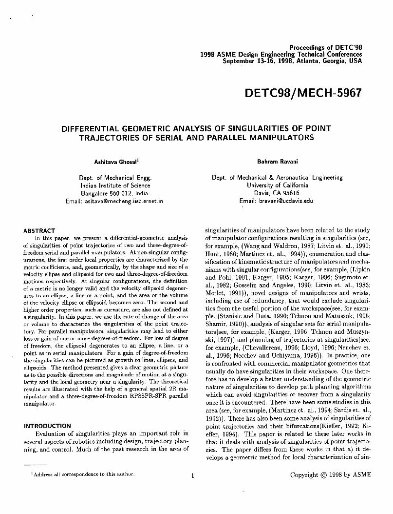
For the values of ~12 = d2 = 1.0 and ~23 = 1.5, the sin- gularities occur for cris = f48.1897‘ and 02 = ?cl31.8103‘. The velocity ellipse for such values degenerates to a straight line along the unit vector (-0.7454, -0.4444, -0.4969)T. Figure 3 shows the three orthographic views of this line and also a 3D view of the degenerate velocity “ellipse”. The

maximum velocity for $ + 4; = 1 is 1.5 along the direction of the straight line. By use of equations (40), one can cal- culate the values of (~12 and 82 for any other set of values of ~12, d2 and ~23 and get plots as in figure 3.

1

0.5

E 0

-0.5

i

-1; -2 -1 0 1 2

vx

1

0.5

: 0 iz

-0.5

-1 -1 -0.5 0 0.5

VY

11

0.5

5 0 ~

-0.5

-1 -2 0 1 -1 2

. . . . . >’ I 1

50

-1

; ” -. I.;,’ a2

VY -1 -2 vx

vx

Figure 3. Degenerate velocity "ellipse" at a singular point

On substituting (~12 and 82 from equations (40) in ex- pressions for gir and giz, we can show that for the general 2R manipulator gii = gis = 0 at a singularity. Since det[g] is independent of 01 all its partial derivatives with respect to 01 is zero. In addition, since gss is constant, all the partial derivatives of gss with respect to 82 are zero. The partial derivative of det[g] with respect to 6’2 is given by

a det bl $722 ~ =911x +922g - 2g12g de2

(41)

9

At the singularity !&$ = 0 and hence the whole of the right-hand side is zero. From equation (30), we obtain that

&(A, . $l)Grl = 0, i,r = 1,2 (42) l=l

Referring to equation (17) and using the above equation, we get at a singularity,

a.$l=O

a. & = 92282 (43)

The above equation implies that acceleration is only possi- ble along the ti2 direction at a singularity.

On computing the second partial derivatives of det[g], we find that the only non-zero term is

a2 det[s] a2g11 ae; = 5’228822 = 2&s; + 44 (44)

The above implies that the singularity in a 2R manipulator is of second order. In addition, the determinant of the ma- trix of second partial derivatives of det[g] is zero implying the singularities are parabolic.

It may be noted that in the planar case, cris = 0 and 82 = 0, A, again the first partial derivatives of det[g] is zero. In the second partial derivatives of det[g], the only non-zero term is

a2 det [s] ae; = 2u2 u2 23 12 (45)

Hence the matrix of second partial derivatives has a zero determinant implying the singularities are parabolic.

A RPSSPR-SbR parallel manipulator

In reference (Lee and Shah, 1988), the three-loop, three- degree-of-freedom RPSSPR-SPR mechanism of figure 4 has been proposed as a “parallel” wrist. The authors have dis- cussed the direct and inverse kinematics but they have not dealt with its singularities. In this subsection, we use the theory developed in section 3, to determine the geometry of the solid region near a singularity for this parallel manipu- lator.

The geometry chosen is same as in (Lee and Shah, 1988) where the revolute joints axes are assumed to be co-planar and are perpendicular to the medians passing through the

Copyright @ 1998 by ASME

0)

x Axis of RI

Figure 4. The RPSSPR-SPR parallel manipulator

respective vertices. Assuming that the length of the medi- ans in the base equilateral triangle are unity, we can obtain the coordinates of the centre of the three spherical joints in the fixed coordinate system (0). These are given by

Sl = [(I - hCl), 0, hs11 T

s2 = [-0.5(1 - Z2c2), X6/2(1 - Zzcz), Z2ss]T (46) s3 = [-0.5(1- Z3c3), -X6/2(1 - Z3c3), Z3s3]T

where Bi, i = 1,2,3 are rotations at the three passive rotary joints and Zi, i = 1,2,3 are the translations at the actuated prismatic joints.

The loop closure equations are obtained from the fact that the distance between the spherical joints are constant and are of the form

(Si - Sj) . (Si - Sj) = kc, i,j = 1,2,3, i # j (47)

where kij is the distance between spherical joint i and spher- ical joint j respectively.

10

Differentiating the three constraint equations with re- spect to time, we get

( 311sr - Z112S~C2 - 2z~z2crss o=. 0 e, +

311Sl - 1113SlC3 - 2ZlZ3ClS3

3/&t - ZlZzClS2 - 211Z2S1C2

3Z2S2 - Z2Z3S2C3 - 2Z2Z3QS3 & $

0

0 3Z3S3 - Z2Z3C2S3 - 2Z2Z352C3 i, +

3Z3S3 - Z1Z3ClS3 - 2ZlZ3SlC3

211 - 3Cl + zscrcs - 2zss1s2 0 i, + 211 - 3Cl + Z3ClC3 - 2Z3SlS3

212 - 3C2 + ZlqC2 - 211~~

2Z2 - SC2 + Z3c2c3 - 2Z3S2S3 i2 +

0

0 2Zs - 3C3 + ZzC2C.3 - 2Zsssss (48) 2Zs - 3~3 + Z1c1c3 - 211s1s3

The above equation can be written in the form of equation (13) as

(2) = +~*I-l[Kl (i) (49)

where the columns of [K*] and [K] are coefficients of bi, i = 1,2,3 and Zi, i = 1,2,3 respectively.

Assuming all the lengths kij’s are &/2(the lengths of the medians of the top platform are 0.5 units each) the coordinates of the centroid of the moving platform are given as

2 0 Y = (l/3)(% + s2 + s3> z

=; [(;lylcl) + (;pi:‘::):I)l

(-l/2)(1 - Z3c3)

+

K

y/2)(1 - Z3C3) )I (5and the velocity of the centre is given by

Copyright @ 1998 by ASME

where [J’] and [J] are 3 x 3 matrices obtained from the coefficients of Bi, i = 1,2,3, and Z;, i = 1,2,3 respectively. Using equation (49) in equation (51), we get

v = ([J] - [J*][K*]-1[l(])(il,i2,i3)T = &,i, (52) i=l

The metric in this case is the matrix ([J] - [J*][lC*]-l[K])T([J]-[J*][K*]-l[K]), and the three-degree- of-freedom RPSSPR-SPR parallel manipulator will loose one or more degree-of-freedom when

det[g*] = ([J] - [J*][K*]-l[II])T([J] - [J*][K*]-‘[Ii]) = 0 (53)

The above equation is a function of the passive variables t$, i = 1,2,3 and the three actuated variables Zi, i = 1,2,3. Equation (53) together with the loop closure equations (47) represent 4 equations in 6 unknowns and hence the singular- ities occur on a high-order 20 surface. It is very difficult to derive analytical results for this case; we, therefore, present numerical results.

At a typical non-singular point given by (11, Zs, Zs) = (0.5, 1.0,2.0) meters, and the corresponding passive variables,(&, 02, es), given by (0.4,0.7535,0.2402 radians, the tip of the velocity vector will lie on the ellipsoid shown in figure 5. The maximum, intermediate, and minimum velocities along the principal axes of the ellip- soid are given by 0.3724,0.3162,0.2031 m/set respectively. The directions of the corresponding principal axes are (0.9921, -0.0394, 0.1187)T, (0.1166,0.6338, -0.7646)T and (-0.0452,0.7724, 0.6335)T respectively.

Prom numerical solution of the constraint equations and the condition for loss of degree-of-freedom, we find that the leg lengths, (Ii, Zs, Zs), given by (0.5,1.0,1.9710) meters and the corresponding passive variables, (01 , 02, es), given by (1.1691,0.4781,0.2355) radians is a singular point. The

11

-0.4 -0.2 0 0.2 0.4 vx

-0.4 :

-0.4 -0.2 0 0.2 0.4

VY

Figure 5. Velocity ellipsoid at a non-singular point

tip of the velocity ellipsoid no longer lies on an ellipsoid and the eigenvalues of the matrix ([J] - [J*][K*]-l[K]) are (0.7647,0,2.2773) / m sec. At this singular point, the mech- anism looses one degree-of-freedom and the velocity distri- bution is the ellipse shown in sectional views and as a 3D plot in figure 6. The centroid of the top platform can move along any direction in a plane spanned by the vectors cor- responding to the two non-zero eigenvalues.

The RPSSPR-SPR parallel manipulator will gain one or more degrees-of-freedom when

det[K*] =

(3ZlSl - Z1Z2S1C2 - 211Z2C1S2) x (&S2 - /2/3S2C3 - 2/2/3C253)

x (3Z3s3 - Z1Z3c1s3 - 2Z1Z3s1c3)

+(311Sl - 11/3QC3 - 2z1/3C1S3) X (3/252 - 11&S2 - 211/2S1Q)

x (313S3 - /2/&S3 - 2/2/&C3) = 0 (54)

The above equation is a function of all the passive and ac- tive joint variables and again together with the loop closure equation (47) represent a set of 4 equations in 6 variables. Thus the singularities resulting in a gain of one or more degrees-of-freedom also lie on a 20 surface. It is very dif- ficult to get the analytical expressions for this surface and we present numerical results.

At leg-lengths, (11, Zz, Zs), g iven by (0.575,0.483,0.544) meters respectively and the corresponding passive variables,

Copyright @ 1998 by ASME

Figure 6. Velocity ellipse at a singular point

(0i, B2, es), given by (-0.3441, -0.0138,0.2320) radians, det[K*] is found to be very close to zero. The eigenvalues of [K*] are -0.5565, 0 and 0.4509 respectively and the three eigenvectors corresponding to the three eigenvalues are (-0.8098,0.3571, -0.4656)T, (-0.3109, -0.8743, -0.3727)T and (-0.0877, -0.4781, -0.8739)T respectively. Hence at this point, the mechanism gains one degree-of-freedom and the velocity of the centroid, with all actuated joints locked, is given as

(55) where the eigenvector, (dr, &, L$$)~, is given as (Y X

(-0.3109, -0.8743, -0.3727)T with CY arbitrary. It is clear that the velocity vector lies along a straight line and the mechanism has gained instantaneously a degree-of-freedom at this singular point. Figure 7 shows the velocity distribu- tion at the singular point.

CONCLUSION

In this paper, we have presented a general geomet- ric framework for differential analysis of point trajectories traced out by multi-degree-of-freedom serial and parallel, non-redundant manipulators. At non-singular points, the

12

0.5 ‘.

20..

-0.5

-1 \ -0.1 -0.05 0 0.05 0.1

Figure 7. Velocity at a singular point

tip of the velocity vector of a point on the end-effector lies on an ellipsoid or ellipse. At singular configurations, the ellipsoid degenerates to an ellipse, a line or a point depend- ing on the number of degrees-of-freedom lost at that point. For a parallel manipulator, at a gain of degree-of-freedom singularity, there is a growth to a line, an ellipse or an ellip- soid depending on the number of degrees-of-freedom gained. In both serial and parallel manipulators, the partial deriva- tives of shape and size of the ellipsoid or ellipse can be used to determine the geometry near the singularity. The devel- oped theory was illustrated with the help of a serial and a parallel manipulator examples.

ACKNOWLEDGMENT

This work was supported by the California Department of Transportation(Caltrans) through the AHMCT research center at UC-Davis.

REFERENCES

Bedrossain, N. S., ‘Classification of singular configura- tion for redundant manipulators’, Proc. of IEEE Conf. on Robotics and Automation, pp. 818-823, 1990.

Chevallereau, C., ‘Feasible trajectories for non redun- dant robot at a singularity’, Proc. of IEEE Conf. on Robotics and Automation, pp. 1871-1876, 1996.

Copyright @ 1998 by ASME

Ghosal, A., and Roth, B., ‘Instantaneous properties of multi-degrees-of-freedom motions - Point trajectories’, Trans. of ASME, Journal of Mechanisms, Transmissions, and Automation in Design, Vol. 109, pp. 107-115, 1987.

Golub, G. H. and Van Loan, C. F., Matrix Computa- tions, Johns Hopkins, 1989.

Gosselin, C. and Angeles, J., ‘Singularity analysis of closed loop kinematic chains’, IEEE Journal of Robotics and Automation, Vol. 6, No. 3, pp. 281-290, 1990.

Hunt, K. H., ‘Special configurations of robot arms via screw theory, Part 1. The Jacobian and its matrix cofactors, Robotica, Vol. 4, pp. 171-179, 1986.

Karger, A., ‘Classification of robot-manipulators with only singularity configurations’, Mechanism and Machine Theory, Vol. 30, pp. 727-736, 1995.

Karger, A., ‘Classification of robot-manipulators with nonremovable singularities’, Trans. of ASME, Journal of Mechanical Design, Vol. 118, pp. 202-208, 1996.

Karger, A., ‘Singularity analysis of serial-robot manip- ulators’, Trans. of ASME, Journal of Mechanical Design, Vol. 118, pp. 520-525, 1996.

Kieffer , J., ‘Manipulator inverse kinematics for untimed end-effector trajectories with singularities’, International Journal of Robotics Research, Vol. 11, No. 3, pp. 225-237, 1992.

Kieffer, J., ‘Differential analysis of bifurcations and iso- lated singularities for robots and mechanisms’, ZEEE Jour- nal of Robotics and Automation, Vol. 10, No. 1, pp. l-10, 1994.

Lee, K. M., and Shah, D., ‘Kinematic analysis of a three-degrees-of-freedom in-parallel actuated manipulator’, IEEE Journal of Robotics and Automation, Vol. 4, No. 3, pp. 354-360, 1988.

Lipkin, H., and Pohl, E., ‘Enumeration of singular configurations for robotic manipulators’, Trans. of ASME, Journal of Mechanical Design, Vol. 113, pp. 272-279, 1991.

Litvin, F. L., Fanghella, P., Tan, J, and Zhang, Y., ‘Sin- gularities in motion and displacement functions of spatial linkages’, Trans. of ASME, Journal of Mechanisms, Trans- missions, and Automation in Design, Vol. 108, pp. 516-523, 1986.

Litvin, F. L., Zhang, Y., Parenti Castelli, V., and In- nocenti, C., ‘Singularities, configurations and displacement functions for manipulators’, The International Journal of Robotics Research, Vol. 5, pp.52-65, 1990.

Lloyd, J. E., ‘Using puiseux series to control non- redundant robots at singularities’, Proc. of IEEE Conf. on Robotics and Automation, pp. 1877-1882, 1996.

Martinez, J. M. R., Alvarado, J. G., and Duffy, J. A., ‘A determination of singular configurations of serial non- redundant manipulators and their escapement from singu- larities using lie products’, Proc. of the Conference on Com-

13

putational Kinematics, Nizza, 1994. Merlet , J .-P., ‘Singularity configurations of parallel ma-

nipulators and Grassman geometry’, International Journal of Robotics Research, Vol. 10, No. 2, pp. 123-134, 1991.

Millman, R. S., and Parker, G. D., Elements of Differ- ential Geome’try, Prentice-Hall Inc., 1977.

Nakamura, Y., Advanced Robotics: Redundancy and Optimization, Addison-Wesley, 1991.

Nenchev, D. N., Tsumaki, Y., Uchiyama, M., Senft, V., and Hirzinger, G., ‘Two approaches to singularity consis- tent motion of nonredundant robotic mechanisms’, Proc. of IEEE Conf. on Robotics and Automation, pp. 1883-1890, 1996.

Nenchev, D. N., and Uchiyama, M., ‘Singularity con- sistent path planning and control of parallel robot motion through instantaneous-self-motion type singularities’, Proc. of IEEE Conf. on Robotics and Automation, pp. 1864-1870, 1996.

Sardis, R., Ravani, B., and Bodduluri, R. M. C., ‘A kinematic design criteriion for singularity avaoidance in re- dundant manipulators’, Proc. of 3rd ARK Conference, pp. 257-261, 1992.

Shamir, T., ‘The singularities of redundant robot arms’, International. Journal of Robotics Research, Vol. 9, No. 1, pp. 113-121, 1990.

Stanisic, M. M., and Duta, O., ‘Symmetrically actu- ated double pointing systems - The basis of singularity free wrists’, IEEE Trans. on Robotics and Automation, Vol. 6, No. 5, pp. 562-569, Oct. 1990.

Sugimoto, K., Duffy, J., and Hunt, K. H. , ‘Special con- figurations of spatial mechanisms and robot arms’, Mecha- nisms and Machine Theory, Vol. 17, pp. 119-132, 1982.

Tchnon, K., and Matuszok, A., ‘On avoiding singularity in redundant robot kinematics’, Robotica, Vol. 13, pp. 599- 606, 1995.

Tchnon, K., and Muszynski, R., ‘Singularities of nonredundant robot kinematics’, International Journal of Robotics Research, Vol. 16, No. 1, pp.60-76, 1997.

Wang, S. L., and Waldron, K. J., ‘A study of the singu- lar configurations of serial manipulators’, Trans. of ASME, Journal of Mechanism, Transmissions and Automation in Design, Vol. 109, pp.14-20, 1987.

Yoshikawa, T., ‘Manipulability of robotic mechanisms’, Robotics Research: The Second International Symposium, MIT Press, pp. 206-214, 1985.

Copyright @ 1998 by ASME