CHAPTER 4 Differentiation and Integration 4.1 INTRODUCTION Given a function f (x) explicitly or defined at a set of n + 1 distinct tabular points, we discuss methods to obtain the approximate value of the rth order derivative f (r) (x), r ≥ 1, at a tabular or a non-tabular point and to evaluate wx a b () z f (x) dx, where w(x) > 0 is the weight function and a and / or b may be finite or infinite. 4.2 NUMERICAL DIFFERENTIATION Numerical differentiation methods can be obtained by using any one of the following three techniques : (i) methods based on interpolation, (ii) methods based on finite differences, (iii) methods based on undetermined coefficients. Methods Based on Interpolation Given the value of f (x) at a set of n + 1 distinct tabular points x 0 , x 1 , ..., x n , we first write the interpolating polynomial P n (x) and then differentiate P n (x), r times, 1 ≤ r ≤ n, to obtain P n r () (x). The value of P n r () (x) at the point x*, which may be a tabular point or a non-tabular point gives the approximate value of f (r) (x) at the point x = x*. If we use the Lagrange interpolating polynomial P n (x) = l xfx i i i n () ( ) = ∑ 0 (4.1) having the error term E n (x) = f (x) – P n (x) = ( )( )...( ) ( )! x x x x x x n n − − − + 0 1 1 f (n+1) (ξ) (4.2) we obtain f (r) (x * ) ≈ P x n r () ( ) ∗ , 1 ≤ r ≤ n and E x n r () ( ) ∗ = f (r) (x * ) – P x n r () ( ) ∗ (4.3) is the error of differentiation. The error term (4.3) can be obtained by using the formula 212
Transcript
CHAPTER 4
Differentiation and Integration
4.1 INTRODUCTION
Given a function f (x) explicitly or defined at a set of n + 1 distinct tabular points, we discussmethods to obtain the approximate value of the rth order derivative f (r) (x), r ≥ 1, at a tabularor a non-tabular point and to evaluate
w xa
b( )� f (x) dx,
where w(x) > 0 is the weight function and a and / or b may be finite or infinite.
4.2 NUMERICAL DIFFERENTIATION
Numerical differentiation methods can be obtained by using any one of the following threetechniques :
(i) methods based on interpolation,(ii) methods based on finite differences,
(iii) methods based on undetermined coefficients.
Methods Based on Interpolation
Given the value of f (x) at a set of n + 1 distinct tabular points x0, x1, ..., xn, we first writethe interpolating polynomial Pn(x) and then differentiate Pn(x), r times, 1 ≤ r ≤ n, to obtain
Pnr( )(x). The value of Pn
r( )(x) at the point x*, which may be a tabular point or a non-tabular pointgives the approximate value of f (r) (x) at the point x = x*. If we use the Lagrange interpolatingpolynomial
Pn(x) = l x f xi ii
n
( ) ( )=∑
0(4.1)
having the error term En(x) = f (x) – Pn(x)
= ( ) ( ) ... ( )
( ) !x x x x x x
nn− − −
+0 1
1 f (n+1) (ξ) (4.2)
we obtain f (r) (x*) ≈ P xnr( ) ( )∗ , 1 ≤ r ≤ n
and E xnr( ) ( )∗ = f (r)(x*) – P xn
r( ) ( )∗ (4.3)
is the error of differentiation. The error term (4.3) can be obtained by using the formula
= c hp + O(hp+1)where c is a constant independent of h, then the method is said to be of order p. Hence, themethods (4.7) and (4.9) are of order 1, whereas the method (4.8) is of order 2.
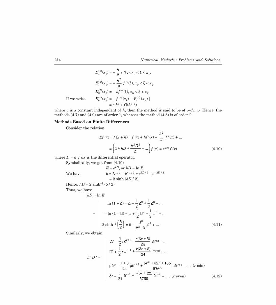
Methods Based on Finite Differences
Consider the relation
Ef (x) = f (x + h) = f (x) + hf ′(x) + h2
2 ! f ″(x) + ...
= 12
2 2
+ + +�
��
hDh D
!... f (x) = e hD f (x) (4.10)
where D = d / dx is the differential operator.Symbolically, we get from (4.10)
E = ehD, or hD = ln E.We have δ = E1 / 2 – E–1 / 2 = ehD / 2 – e– hD / 2
= 2 sinh (hD / 2).Hence, hD = 2 sinh–1 (δ / 2).Thus, we have
hD = ln E
ln (1 + ∆) = ∆ – 12
13
2 3∆ ∆+ – ...
= – ln (1 – ∇ ) = ∇ + 12
13
2 3∇ + ∇ + ...
2 sinh–1 δ2��� = δ –
12 3
2
23
. !δ + ... (4.11)
Similarly, we obtain
∆r – 12
3 524
1rr rr∆ + + +( )
∆r+2 – ...
∇ r + 12
3 524
1rr rr∇ + ++ ( )
∇ r+2 + ...hr D r =
µδ r – r r rr+ + + ++324
5 52 1355760
22
µδ µδ r+4 – ..., (r odd)
δ r – r r rr r
245 225760
2 4δ δ+ ++ +( ) – ..., (r even) (4.12)
8-\N-NUM\NU-4-1
Differentiation and Integration 215
where, µ = 14
2
+�
��
δ is the averaging operator and is used to avoid off-step points in the
method.Retaining various order differences in (4.12), we obtain different order methods for a
given value of r. Keeping only one term in (4.12), we obtain for r = 1 (fk+1 – fk) / h, ...[4.13 (i)]
The methods (4.13i), (4.13ii), (4.14i), (4.14ii) are of first order, whereas the methods(4.13iii) and (4.14iii) are of second order.
Methods Based on Undetermined CoefficientsWe write
hr f (r)(xk ) = a f xi k ii m
m
( )+= −∑ (4.15)
for symmetric arrangement of tabular points and
hr f (r)(xk ) = a f xi k ii m
n
( )+= ±∑ (4.16)
for non symmetric arrangement of tabular points.The error term is obtained as
Er(xk ) = 1
hr [hr f (r) (xk ) – Σai f (xk+i )]. (4.17)
The coefficients ai’s in (4.15) or (4.16) are determined by requiring the method to be of aparticular order. We expand each term in the right side of (4.15) or (4.16) in Taylor seriesabout the point xk and on equating the coefficients of various order derivatives on both sides,we obtain the required number of equations to determine the unknowns. The first non-zeroterm gives the error term.
For m = 1 and r = 1 in (4.15), we obtain hf ′(xk ) = a–1 f (xk–1) + a0 f (xk ) + a1f (xk+1)
Comparing the coefficients of f (xk), hf ′(xk) and (h2 / 2) f ″(xk) on both sides, we geta–1 + a0 + a1 = 0, – a–1 + a1 = 1, a–1 + a1 = 0
whose solution is a0 = 0, a–1 = – a1 = – 1 / 2. We obtain the formula
h fk′ = 12
(fk+1 – fk–1), or fk′ = 1
2h (fk+1 – fk–1). (4.18)
8-\N-NUM\NU-4-1
216 Numerical Methods : Problems and Solutions
The error term in approximating f ′(xk) is given by (– h2 / 6) f ″′ (ξ), xk–1 < ξ < xk+1.For m = 1 and r = 2 in (4.15), we obtain
h2 f ″(xk ) = a–1 f (xk–1) + a0 f (xk ) + a1 f (xk+1)= (a–1 + a0 + a1) f (xk ) + (– a–1 + a1) hf ′(xk )
+ 12
(a–1 + a1) h2 f ″(xk ) +
16
(– a–1 + a1) h3 f ″′ (xk )
+ 1
24 (a–1 + a1) h
4 f iv(xk ) + ......
Comparing the coefficients of f (xk ), hf ′(xk ) and h2 f ″(xk ) on both sides, we geta–1 + a0 + a1 = 0, – a–1 + a1 = 0, a–1 + a1 = 2
whose solution is a–1 = a1 = 1, a0 = – 2. We obtain the formula
h2 fk″ = fk–1 – 2fk + fk+1, or fk″ = 12h
(fk–1 – 2fk + fk+1). (4.19)
The error term in approximating f ″(xk ) is given by (– h2 / 12) f (4) (ξ), xk–1 < ξ < xk+1.Formulas (4.18) and (4.19) are of second order.Similarly, for m = 2 in (4.15) we obtain the fourth order methods
with the error terms (h4 / 30) f v(ξ) and (h4 / 90) f vi (ξ) respectively and xk–2 < ξ < xk+2.
4.3 EXTRAPOLATION METHODS
To obtain accurate results, we need to use higher order methods which require a large numberof function evaluations and may cause growth of roundoff errors. However, it is generallypossible to obtain higher order solutions by combining the computed values obtained by usinga certain lower order method with different step sizes.
If g(x) denotes the quantity f (r) (xk) and g(h) and g(qh) denote its approximate valueobtained by using a certain method of order p with step sizes h and qh respectively, we have
g(h) = g(x) + chp + O(hp+1), (4.22) g(qh) = g(x) + c qp hp + O(hp+1). (4.23)
Eliminating c from (4.22) and (4.23) we get
g(x) = q g h g qh
q
p
p( ) ( )−
− 1 + O(hp+1) (4.24)
which defines a method of order p + 1. This procedure is called extrapolation or Richardson’sextrapolation.
If the error term of the method can be written as a power series in h, then by repeatingthe extrapolation procedure a number of times, we can obtain methods of higher orders. Weoften take the step sizes as h, h / 2, h / 22, .... If the error term of the method is of the form
E(xk ) = c1h + c2h2 + ... (4.25)then, we have
g(h) = g(x) + c1h + c2h2 + ... (4.26)
Writing (4.26) for h, h / 2, h / 22, ... and eliminating ci’s from the resulting equations, weobtain the extrapolation scheme
8-\N-NUM\NU-4-1
Differentiation and Integration 217
g (p)(h) = 2 2
2 1
1 1p p p
pg h g h( ) ( )( / ) ( )− −−
−, p = 1, 2, ... (4.27)
where g (0) (h) = g(h).The method (4.27) has order p + 1.The extrapolation table is given below.
The extrapolation procedure can be stopped when| g(k) (h) – g(k–1) (h / 2) | < ε
where ε is the prescribed error tolerance.
4.4 PARTIAL DIFFERENTIATION
One way to obtain numerical partial differentiation methods is to consider only one variable ata time and treat the other variables as constants. We obtain
∂∂���
fx x yi j( , )
= ( )/ ( ),( )/ ( ),( )/( ) ( ),
, ,
, ,
, ,
f f h O hf f h O hf f h O h
i j i j
i j i j
i j i j
+
−
+ −
− +− +
− +
1
1
1 122
(4.31)
8-\N-NUM\NU-4-1
218 Numerical Methods : Problems and Solutions
∂∂��� =
− +− +
− +
+
−
+ −
fy
f f k O kf f k O kf f k O kx y
i j i j
i j i j
i j i ji j( , )
, ,
, ,
, ,
( )/ ( ),( )/ ( ),( )/( ) ( ),
1
1
1 122
(4.32)
where h and k are the step sizes in x and y directions respectively.Similarly, we obtain
∂∂
�
��
2
2f
x x yi j( , ) = (fi–1, j – 2fi, j + fi+1, j ) / h2 + O(h2),
∂∂
�
��
2
2f
y x yi j( , ) = (fi, j+1 – 2fi, j + fi, j–1) / k2 + O(k2),
In numerical differentiation methods, error of approximation or the truncation error is of theform chp which tends to zero as h → 0. However, the method which approximates f (r)(x) con-tains hr in the denominator. As h is successively decreased to small values, the truncationerror decreases, but the roundoff error in the method may increase as we are dividing by asmaller number. It may happen that after a certain critical value of h, the roundoff error maybecome more dominant than the truncation error and the numerical results obtained maystart worsening as h is further reduced. When f (x) is given in tabular form, these values maynot themselves be exact. These values contain roundoff errors, that is f (xi ) = fi + εi, where f (xi )is the exact value and fi is the tabulated value. To see the effect of this roundoff error in anumerical differentiation method, we consider the method
f ′(x0) = f x f x
hh( ) ( )
–1 0
2−
f ″(ξ), x0 < ξ < x1. (4.34)
If the roundoff errors in f (x0) and f (x1) are ε0 and ε1 respectively, then we have
f ′(x0) = f f
h hh1 0 1 0
2−
+−
−ε ε
f ″(ξ) (4.35)
or f ′(x0) = f f
h1 0−
+ RE + TE (4.36)
where RE and TE denote the roundoff error and the truncation error respectively. If we take
ε = max ( | ε1 |, | ε2 |), and M2 = maxx x x0 1≤ ≤ | f ″(x) |
then, we get | RE | ≤ 2εh
, and | TE | ≤ h2
M2.
We may call that value of h as an optimal value for which one of the following criteria issatisfied :
(i) | RE | = | TE | [4.37 (i)](ii) | RE | + | TE | = minimum. [4.37 (ii)]
8-\N-NUM\NU-4-1
Differentiation and Integration 219
If we use the criterion [4.37(i)], then we have
2
2ε
hh= M2
which gives hopt = 2 ε/M2 , and | RE | = | TE | = ε M2 .
If we use the criterion [4.37 (ii)], then we have2
2 2ε
hh
M+ = minimum
which gives – 2 122 2
εh
M+ = 0, or hopt = 2 ε/M2 .
The minimum total error is 2(εM2)1 / 2.
This means that if the roundoff error is of the order 10–k (say) and M2 ≈ 0(1), then theaccuracy given by the method may be approximately of the order 10–k / 2. Since, in any numeri-cal differentiation method, the local truncation error is always proportional to some power ofh, whereas the roundoff error is inversely proportional to some power of h, the same techniquecan be used to determine an optimal value of h, for any numerical method which approximatesf (r) (xk ), r ≥ 1.
4.6 NUMERICAL INTEGRATION
We approximate the integral
I = w x f x dxa
b( ) ( )� (4.38)
by a finite linear combination of the values of f (x) in the form
I = w x f x dx f xa
b
k kk
n
( ) ( ) ( )� ∑==
λ0
.(4.39)
where xk, k = 0(1)n are called the abscissas or nodes which are distributed within the limits ofintegration [a, b] and λk, k = 0(1)n are called the weights of the integration method or thequadrature rule (4.39). w(x) > 0 is called the weight function. The error of integration is givenby
Rn = w x f x dx f xk kk
n
a
b( ) ( ) ( )−
=∑� λ
0. .(4.40)
An integration method of the form (4.39) is said to be of order p, if it produces exactresults (Rn ≡ 0), when f (x) is a polynomial of degree ≤ p.
Since in (4.39), we have 2n + 2 unknowns (n + 1 nodes xk’s and n + 1 weights λk’s), themethod can be made exact for polynomials of degree ≤ 2n +1. Thus, the method of the form(4.39) can be of maximum order 2n + 1. If some of the nodes are known in advance, the orderwill be reduced.
For a method of order m, we have
w x x dx xik k
i
k
n
a
b( ) −
=∑� λ
0
= 0, i = 0, 1, ..., m (4.41)
which determine the weights λk’s and the abscissas xk’s. The error of integration is obtainedfrom
8-\N-NUM\NU-4-1
220 Numerical Methods : Problems and Solutions
Rn = C
m( ) !+ 1 f (m+1) (ξ), a < ξ < b, (4.42)
where C = w x x dx xa
bm
k km
k
n
( )� ∑+ +
=
−1 1
0
λ . (4.43)
4.7 NEWTON-COTES INTEGRATION METHODS
In this case, w(x) = 1 and the nodes xk’s are uniformly distributed in [a, b] with x0 = a, xn = band the spacing h = (b – a) / n. Since the nodes xk’s, xk = x0 + kh, k = 0, 1, ..., n, are known, wehave only to determine the weights λk’s, k = 0, 1, ..., n. These methods are known as Newton-Cotes integration methods and have the order n. When both the end points of the interval ofintegration are used as nodes in the methods, the methods are called closed type methods,otherwise, they are called open type methods.
Closed type methods
For n = 1 in (4.39), we obtain the trapezoidal rule
f x dxh
a
b( ) =� 2
[f (a) + f (b)] (4.44)
where h = b – a. The error term is given as
R1 = – h3
12 f ″(ξ), a < ξ < b. (4.45)
For n = 2 in (4.39), we obtain the Simpson’s rule
f x dxh
f a fa b
f ba
b( ) ( ) ( )= + +�
�� +�
������ 3
42
(4.46)
where h = (b – a)2. The error term is given by
R2 = C3 !
f ″′ (ξ), a < ξ < b.
We find that in this case
C = x dxb a
aa b
ba
b3 3
33
64
2− − + +�
�� +
�
���
�
���� ( ) = 0
and hence the method is exact for polynomials of degree 3 also. The error term is now given by
R2 = C4 ! f iv(ξ), a < ξ < b.
We find that C = x dxb a
aa b
bb a
a
b4 4
44
5
64
2 120� −−
++�
�� +
�
���
�
���
= −−( ) ( )
.
Hence, the error of approximation is given by
R2 = – ( )
( )b a
fhiv− = −
5 5
2880 90ξ f iv(ξ), a < ξ < b. (4.47)
since h = (b – a) / 2.For n = 3 in (4.39), we obtain the Simpson’s 3 / 8 rule
8-\N-NUM\NU-4-1
Differentiation and Integration 221
f x dxh
a
b( ) =� 3
8 [f (a) + 3f (a + h) + 3f (a + 2h) + f (b)] (4.48)
where h = (b – a) / 3. The error term is given by
R3 = – 380
h5 f iv (ξ), a < ξ < b, (4.49)
and hence the method (4.49) is also a third order method.The weights λk’s of the Newton-Cotes rules for n ≤ 5 are given in Table 4.3. For large n,
some of the weights become negative. This may cause loss of significant digits due to mutualcancellation.
Table 4.3. Weights of Newton-Cotes Integration Rule (4.39)
where the end points x0 = a and xn = b are excluded.For n = 2, we obtain the mid-point rule
f x dx h f a ba
b( ) ( )= +� 2 (4.51)
where h = (b – a) / 2. The error term is given by
R2 = h
f3
3″ ( )ξ .
Similarly, for different values of n and h = (b – a) / n, we obtain
n = 3 : I = 32h
[f (a + h) + f (a + 2h)].
R3 = 34
h3 f ″(ξ). (4.52)
n = 4 : I = 43h
[2f (a + h) – f (a + 2h) + 2f (a + 3h)].
R4 = 1445
h5 f iv(ξ). (5.53)
n = 5 : I = 524h
[11f (a + h) + f (a + 2h) + f (a + 3h) + 11f (a + 4h)].
R5 = 95
144 h5 f iv(ξ), (4.54)
where a < ξ < b.
8-\N-NUM\NU-4-1
222 Numerical Methods : Problems and Solutions
4.8 GAUSSIAN INTEGRATION METHODS
When both the nodes and the weights in the integration method (4.39) are to be determined,then the methods are called Gaussian integration methods.
If the abscissas xk’s in (4.39) are selected as zeros of an orthogonal polynomial, orthogonalwith respect to the weight function w(x) on the interval [a, b], then the method (4.39) has order2n + 1 and all the weights λk > 0.
The proof is given below.Let f (x) be a polynomial of degree less than or equal to 2n + 1. Let qn(x) be the Lagrange
interpolating polynomial of degree ≤ n, interpolating the data (xi, fi ), i = 0, 1, ..., n
qn(x) = l x f xk kk
n
( ) ( )=∑
0
with lk(x) = π
π( )
( ) ( )x
x x xk k− ′.
The polynomial [f (x) – qn(x)] has zeros at x0, x1, ... xn. Hence, it can be written asf (x) – qn(x) = pn+1(x) rn(x)
where rn(x) is a polynomial of degree atmost n and pn+1(xi ) = 0, i = 0, 1, 2, ... n. Integrating thisequation, we get
w xa
b( )� [f (x) – qn(x)] dx = w x
a
b( )� pn+1(x) rn(x) dx
or w x f x dx w x q x dx w xna
b
a
b
a
b( ) ( ) ( ) ( ) ( )= + ��� pn+1(x) rn(x) dx.
The second integral on the right hand side is zero, if pn+1 (x) is an orthogonal polyno-mial, orthogonal with respect to the weight function w(x), to all polynomials of degree lessthan or equal to n.
We then have
w x f x dx w x q x dx f xn k kk
n
a
b
a
b( ) ( ) ( ) ( ) ( )= =
=∑�� λ
0
where λk = w x l x dxka
b( ) ( ) .�
This proves that the formula (4.39) has precision 2n + 1.
Observe that l xj2 ( ) is a polynomial of degree less than or equal to 2n.
Choosing f (x) = l xj2 ( ) , we obtain
w x l x dx l xja
b
k j kk
n
( ) ( ) ( )2 2
0� ∑=
=
λ .
Since lj(xk ) = δjk, we get
λj = w x l x dxja
b( ) ( )2� > 0.
Since any finite interval [a, b] can be transformed to [– 1, 1], using the transformation
x = ( ) ( )b a
tb a− + +
2 2we consider the integral in the form
8-\N-NUM\NU-4-1
Differentiation and Integration 223
w x f x dx f xk kk
n
( ) ( ) ( )==
− ∑� λ0
1
1
. (4.55)
Gauss-Legendre Integration MethodsWe consider the integration rule
f x dx f xk kk
n
( ) ( )==
−∑� λ
01
1. (4.56)
The nodes xk’s are the zeros of the Legendre polynomials
Pn+1(x) = 1
2 11
1
1n
n
nnddx+
+
++( ) ! [(x2 – 1)n+1]. (4.57)
The first few Legendre polynomials are given by P0(x) = 1, P1(x) = x, P2(x) = (3x2 – 1) / 2, P3(x) = (5x3 – 3x) / 2, P4(x) = (35x4 – 30x2 + 3) / 8.
The Legendre polynomials are orthogonal on [– 1, 1] with respect to the weight functionw(x) = 1. The methods (4.56) are of order 2n + 1 and are called Gauss-Legendre integrationmethods.
For n = 1, we obtain the method
f x dx f f( ) = −�
��
+��� −� 1
3
1
31
1
(4.58)
with the error term (1 / 135) f (4) (ξ), – 1 < ξ < 1.For n = 2, we obtain the method
−� = − + +1
1 19
5 3 5 8 0 5 3 5f x dx f f f( ) [ ( / ) ( ) ( / )] (4.59)
with the error term (1 / 15750) f (6) (ξ), – 1 < ξ < 1.The nodes and the corresponding weights of the method (4.56) for n ≤ 5 are listed in
Table 4.4.Table 4.4. Nodes and Weights for the Gauss-Legendre Integration Methods (4.56)
In this case, w(x) = 1 and the two end points – 1 and 1 are always taken as nodes. Theremaining n – 1 nodes and the n + 1 weights are to be determined. The integration methods ofthe form
−=
−
� ∑= − + +1
1
01
1
1 1f x dx f f x fk k nk
n
( ) ( ) ( ) ( )λ λ λ (4.60)
are called the Lobatto integration methods and are of order 2n – 1.For n = 2, we obtain the method
−� =1
1 13
f x dx( ) [f (– 1) + 4f (0) + f (1)] (4.61)
with the error term (– 1 / 90) f (4)(ξ), – 1 < ξ < 1.The nodes and the corresponding weights for the method (4.60) for n ≤ 5 are given in
Table 4.5.Table 4.5. Nodes and Weights for Lobatto Integration Method (4.60)
In this case, w(x) = 1 and the lower limit – 1 is fixed as a node. The remaining n nodesand n + 1 weights are to be determined. The integration methods of the form
−
=� ∑= − +
1
1
01
1f x dx f f xk kk
n
( ) ( ) ( )λ λ (4.62)
are called Radau integration methods and are of order 2n.For n = 1, we obtain the method
−� = − + ��� 1
1 12
132
13
f x dx f f( ) ( ) (4.63)
with the error term (2 / 27) f ″′ (ξ), – 1 < ξ < 1.For n = 2, we obtain the method
−� 1
1f x dx( ) =
29
116 6
181 6
516 6
181 6
5f f f( )− + + −�
��
+ − +�
��
(4.64)
with the error term (1 / 1125) f (5) (ξ), – 1 < ξ < 1.
8-\N-NUM\NU-4-2
Differentiation and Integration 225
The nodes and the corresponding weights for the method (4.62) are given in Table 4.6.Table 4.6. Nodes and Weights for Radau Integration Method (4.62)
The Chebyshev polynomials are orthogonal on [– 1, 1] with respect to the weight func-
tion w(x) = 1 / 1 2− x . The methods of the form (4.65) are called Gauss-Chebyshev integrationmethods and are of order 2n + 1.
8-\N-NUM\NU-4-2
226 Numerical Methods : Problems and Solutions
We obtain from (4.66)
xk = cos ( )2 1
2 1kn++
�
��
π, k = 0.1, ..., n. (4.67)
The weights λk’s in (4.65) are equal and are given by
λk = π
n + 1, k = 0, 1, ..., n. (4.68)
For n = 1, we obtain the method
−� −
= −�
�� +
���
���
���
1
1
21 21
2
1
2
f x
xdx f f
( ) π(4.69)
with the error term (π / 192) f (4)(ξ), – 1 < ξ < 1.
For n = 2, we obtain the method
−� −= −
�
��
+ +���
�
���
�
���1
1
2
1
1 33
20
32x
f x dx f f f( ) ( )π
(4.70)
with the error term (π / 23040) f (6) (ξ), – 1 < ξ < 1.
Gauss-Laguerre Integration Methods
We consider the integral
0
0
∞ −
=� ∑=e f x dx f xx
k kk
n
( ) ( )λ (4.71)
where w(x) = e–x is the weight function. The nodes xk’s are the zeros of the Laguerre polynomial
Ln+1(x) = (– 1)n+1 ex d
dx
n
n
+
+
1
1 [e–x xn+1] (4.72)
The first few Laguerre polynomials are given by
L0(x) = 1, L1(x) = x – 1, L2(x) = x2 – 4x + 2,
L3(x) = x3 – 9x2 + 18x – 6.
The Laguerre polynomials are orthogonal on [0, ∞) with respect to the weight functione–x. The methods of the form (4.71) are called Gauss-Laguerre integration method and are oforder 2n + 1.
For n = 1, we obtain the method
0
2 24
2 22 2
42 2
∞ −� = + − + − +e f x dx f fx ( ) ( ) ( ) (4.73)
with the error term (1 / 6) f (4) (ξ), – 1 < ξ < 1.
The nodes and the weights of the method (4.71) for n ≤ 5 are given in Table 4.7.
8-\N-NUM\NU-4-2
Differentiation and Integration 227
Table 4.7. Nodes and Weights for Gauss-Laguerre Integration Method (4.71)
To avoid the use of higher order methods and still obtain accurate results, we use the compos-ite integration methods. We divide the interval [a, b] or [– 1, 1] into a number of subintervalsand evaluate the integral in each subinterval by a particular method.
Composite Trapezoidal Rule
We divide the interval [a, b] into N subintervals [xi–1, xi ], i = 1, 2, ..., N, each of lengthh = (b – a) / N, x0 = a, xN = b and xi = x0 + ih, i = 1, 2, ..., N – 1. We write
f x dx f x dx f x dx f x dxx
x
x
x
x
x
a
b
N
N( ) ( ) ( ) ... ( )= + + +
−����
11
2
0
1. (4.78)
Evaluating each of the integrals on the right hand side of (4.78) by the trapezoidal rule(4.44), we obtain the composite rule
f x dxh
a
b( ) =� 2
[f0 + 2(f1 + f2 + ... + fN–1) + fN ] (4.79)
where fi = f (xi ).The error in the integration method (4.79) becomes
R1 = – h3
12 [f ″(ξ1) + f ″(ξ2) + ... + f ″(ξN )], xi–1 < ξi < xi. (4.80)
Denoting f ″(η) = max
a x b≤ ≤ | f ″(x) |, a < η < b
8-\N-NUM\NU-4-2
Differentiation and Integration 229
we obtain from (4.80)
| R1 | ≤ Nh3
12 f ″(η) =
( )( )
( )b a
Nf
b a− ″ = −3
212 12η h2 f ″(η). (4.81)
Composite Simpson’s Rule
We divide the interval [a, b] into 2N subintervals each of length h = (b – a) / (2N). Wehave 2N + 1 abscissas x0, x1, ..., x2N with x0 = a, x2N = b, xi = x0 + ih, i = 1, 2, ..., 2N – 1.
We write
f x dx f x dx f x dx f x dxx
x
x
x
x
x
a
b
N
N( ) ( ) ( ) ... ( )= + + +
−����
2 2
2
2
4
0
2. (4.82)
Evaluating each of the integrals on the right hand side of (4.82) by the Simpson’s rule(4.46), we obtain the composite rule
(4.83)The error in the integration method (4.83) becomes
R2 = – h5
90 [f iv(ξ1) + f iv(ξ2) + ... + f iv(ξN)], x2i–2 < ξi < x2i (4.84)
Denoting f iv(η) = maxa x b≤ ≤
| f iv(x) |, a < η < b
we obtain from (4.84)
| R2 | ≤ Nhf
b a
Nf
b aiv iv5 5
490 2880 180( )
( )( )
( )η η=−
=− h4 f iv(η) (4.85)
4.10 ROMBERG INTEGRATION
Extrapolation procedure of section 4.3, applied to the integration methods is called Rombergintegration. The errors in the composite trapezoidal rule (4.79) and the composite Simpson’srule (4.83) can be obtained as
I = IT + c1h2 + c2h4 + c3h
6 + ... (4.86) I = IS + d1h
4 + d2h6 + d3h8 + ... (4.87)
respectively, where ci’s and di’s are constants independent of h.Extrapolation procedure for the trapezoidal rule becomes
I hI h I h
Tm
mTm
Tm
m( )
( ) ( )
( )( / ) ( )
=−
−
− −4 24 1
1 1
, m = 1, 2,... (4.88)
where I hT( ) ( )0 = IT (h).
The method (4.88) has order 2m + 2.Extrapolation procedure for the Simpson’s rule becomes
I hI h I h
Sm
mSm
Sm
m( )
( ) ( )
( )( / ) ( )
=−
−
+ − −
+
4 2
4 1
1 1 1
1 , m = 1, 2,... (4.89)
where IS( )0 (h) = IS (h).
The method (4.89) has order 2m + 4.
8-\N-NUM\NU-4-2
230 Numerical Methods : Problems and Solutions
4.11 DOUBLE INTEGRATION
The problem of double integration is to evaluate the integral of the form
I = f x y dx dyc
d
a
b( , )�� . (4.90)
This integral can be evaluated numerically by two successive integrations in x any ydirections respectively, taking into account one variable at a time.
Trapezoidal ruleIf we evaluate the inner integral in (4.90) by the trapezoidal rule, we get
IT = d cf x c f x d dx
a
b−+�2
[ ( , ) ( , )] . (4.91)
Using the trapezoidal rule again in (4.91) we get
IT = ( ) ( )b a d c− −
4 [f (a, c) + f (b, c) + f (a, d) + f (b, d)]. (4.92)
The composite trapezoidal rule for evaluating (4.90) can be written as
where h and k are the spacings in x and y directions respectively and h = (b – a) / N, k = (d – c) / M, xi = x0 + ih, i = 1, 2, ..., N – 1, yj = y0 + jk, j = 1, 2, ..., M – 1,x0 = a, xN = b, y0 = c, yM = d.
The computational molecule of the method (4.93) for M = N = 1 and M = N = 2 can bewritten as
Trapezoidal rule Composite trapezoidal rule
Simpson’s rule
If we evaluate the inner integral in (4.90) by Simpson’s rule then we get
IS = k
f x c f x c k f x d dxa
b
34[ ( , ) ( , ) ( , )]+ + +� (4.94)
where k = (d – c) / 2.
8-\N-NUM\NU-4-2
Differentiation and Integration 231
Using Simpson’s rule again in (4.94), we get
IS = hk9
[f (a, c) + f (a, d) + f (b, c) + f (b, d)
+ 4{f (a + h, c) + f (a + h, d) + f (b, c + k)+ f (a, c + k)} + 16f (a + h, c + k)] (4.95)
where h = (b – a) / 2.The composite Simpson’s rule for evaluating (4.90) can be written as
IS = hk
f f f fi i Ni
N
i
N
94 200 2 1 0 2 0 2 0
1
1
1
+ + +�����
�����
�
��� −
=
−
=∑∑ , , ,
+ 4 f f f fj i j i j N ji
N
i
N
j
M
0 2 1 2 1 2 1 2 2 1 2 2 11
1
11
4 2, , , ,− − − − −=
−
==
+ + +�����
�����
∑∑∑
+ 2 f f f fj i j i j N ji
N
i
N
j
M
0 2 2 1 2 2 2 2 21
1
11
1
4 2, , , ,+ + +�����
�����
−=
−
==
−
∑∑∑
+ f f f fM i M i M N Mi
N
i
N
0 2 2 1 2 2 2 2 21
1
1
4 2, , , ,+ + +�����
�����
−=
−
=∑∑ (4.96)
where h and k are the spacings in x and y directions respectively andh = (b – a) / (2N), k = (d – c) / (2M),xi = x0 + ih, i = 1, 2, ..., 2N – 1,yj = y0 + jk, j = 1, 2, ..., 2M – 1,
x0 = a, x2N = b, y0 = c, y2M = d.The computational module for M = N = 1 and M = N = 2 can be written as
Simpson’s rule Composite Simpson’s rule
4.12 PROBLEMS AND SOLUTIONS
Numerical differentiation
4.1 A differentiation rule of the formf ′(x0) = α0 f0 + α1 f1 + α2 f2,
where xk = x0 + kh is given. Find the values of α0, α1 and α2 so that the rule is exact forf ∈ P2. Find the error term.
8-\N-NUM\NU-4-2
232 Numerical Methods : Problems and Solutions
SolutionThe error in the differentiation rule is written as
TE = f ′(x0) – α0 f (x0) – α1 f (x1) – α2 f (x2).Expanding each term on the right side in Taylor’s series about the point x0, we obtain
TE = – (α0 + α1 + α2) f (x0) + (1 – h(α1 + 2α2)) f ′(x0)
– h2
2 (α1 + 4α2) f ″(x0) –
h3
6 (α1 + 8α2) f ″′ (x0) – ...
We choose α0, α1 and α2 such thatα0 + α1 + α2 = 0,
α1 + 2α2 = 1 / h, α1 + 4α2 = 0.
The solution of this system isα0 = – 3 / (2h), α1 = 4 / (2h), α2 = – 1 / (2h).
Hence, we obtain the differentiation rulef ′(x0) = (– 3f0 + 4f1 – f2) / (2h)
with the error term
TE = h3
1 268( )α α+ f ″′ (ξ) = –
h2
3 f ″′ (ξ), x0 < ξ < x2.
The error term is zero if f (x) ∈ P2. Hence, the method is exact for all polynomials ofdegree ≤ 2.
4.2. Using the following data find f ′(6.0), error = O(h), and f ″(6.3), error = O(h2)
x 6.0 6.1 6.2 6.3 6.4
f (x) 0.1750 – 0.1998 – 0.2223 – 0.2422 – 0.2596
SolutionMethod of O(h) for f ′(x0) is given by
f ′(x0) = 1
0 0hf x h f x[ ( ) ( )]+ −
With x0 = 6.0 and h = 0.1, we get
f ′(6.0) = 1
0 1. [ f (6.1) – f (6.0)]
= 1
0 1. [– 0.1998 – 0.1750] = – 3.748.
Method of O(h2) for f ″(x0) is given by
f ″(x0) = 12h
[ f (x0 – h) – 2f (x0) + f (x0 + h)]
With x0 = 6.3 and h = 0.1, we get
f ″(6.3) = 1
1 2( )0. [ f (6.2) – 2f (6.3) + f (6.4)] = 0.25.
8-\N-NUM\NU-4-2
Differentiation and Integration 233
4.3 Assume that f (x) has a minimum in the interval xn–1 ≤ x ≤ xn+1 where xk = x0 + kh. Showthat the interpolation of f (x) by a polynomial of second degree yields the approximation
fn – 18 2
1 12
1 1
( )f ff f f
n n
n n n
+ −
+ −
−− +
�
��
, fk = f (xk)
for this minimum value of f (x). (Stockholm Univ., Sweden, BIT 4 (1964), 197)SolutionThe interpolation polynomial through the points (xn–1, fn–1), (xn, fn) and (xn+1, fn+1) isgiven as
(b) Calculate y′(0.398) as accurately as possible using the table below and with the aid ofthe approximation S(h). Give the error estimate (the values in the table are correctlyrounded).
x 0.398 0.399 0.400 0.401 0.402
f (x) 0.408591 0.409671 0.410752 0.411834 0.412915
(Royal Inst. Tech. Stockholm, Sweden, BIT 19(1979), 285)Solution(a) Expanding each term in the formula
with h = 0.4, 0.2, 0.1.(Royal Inst. Tech., Stockhlom, Sweden, BIT 6 (1966), 270)
SolutionApplying the Richardson’s extrapolation formula
ff f
ii h
ii h i h
i,– , – ,–
–, , ,...′ =
′ ′=
4
4 11 21 1 2
where i denotes the ith iterate, we obtain
8-\N-NUM\NU-4-3
Differentiation and Integration 239
h O(h2) O(h4) O(h6)
0.4 0.5260100.540274
0.2 0.536708 0.5402990.540297
0.1 0.539400
4.10 The formulaDh = (2h)–1 (3 f (a) – 4 f (a – h) + f (a – 2h))
is suitable to approximation of f ′(a) where x is the last x-value in the table.(a) State the truncation error Dh – f ′(a) as a power series in h.(b) Calculate f ′(2.0) as accurately as possible from the table
Using the extrapolation scheme, we obtain the following extrapolation table.Extrapolation Table
h O(h2) O(h3) O(h4) O(h5)
0.4 0.4366180.458654
0.2 0.453145 0.4593520.459265 0.459402
0.1 0.457735 0.4593990.459382
0.05 0.458970
Hence, f ′(2.0) = 0.4594 with the error 2.0 × 10⁻⁶.
8-\N-NUM\NU-4-3
240 Numerical Methods : Problems and Solutions
4.11 For the method
f ′(x0) = − + −
+3 4
2 30 1 2
2f x f x f xh
h( ) ( ) ( ) f ″′ (ξ), x0 < ξ < x2
determine the optimal value of h, using the criteria(i) | RE | = | TE |,
(ii) | RE | +| TE | = minimum.Using this method and the value of h obtained from the criterion | RE | = | TE |,determine an approximate value of f ′(2.0) from the following tabulated values off (x) = loge x
x 2.0 2.01 2.02 2.06 2.12
f (x) 0.69315 0.69813 0.70310 0.72271 0.75142
given that the maximum roundoff error in the function evaluations is 5 × 10⁻⁶.SolutionIf ε0, ε1 and ε2 are the roundoff errors in the given function evaluations f0, f1 and f2respectively, then we have
f ′(x0) = − + −
+− + −
+3 4
23 4
2 30 1 2 0 1 2
2f f fh h
hε ε ε f ″′ (ξ)
= − + −3 4
20 1 2f f f
h + RE + TE.
Using ε = max (| ε0 |, | ε1 |, | ε2 |),
and M3 = maxx x x0 2≤ ≤ | f ″′ (x) |,
we obtain | RE | ≤ 82 3
23ε
hh M
, | |TE ≤ .
If we use | RE | = | TE |, we get
82 3
23ε
hh M
=
which gives h3 = 12
3
εM
, or hopt = 12
3
1/3ε
M�
��
and | RE | = | TE | = 4
12
2 331/3
1/3
ε /
( )
M.
If we use | RE | + | TE | = minimum, we get
433
2εh
M h+ = minimum
which gives − +4 2
323ε
h
M h = 0, or hopt =
6
3
1/3ε
M�
��
.
Minimum total error = 62/3 ε2/3 M31/3 .
8-\N-NUM\NU-4-3
Differentiation and Integration 241
When, f (x) = loge (x), we have
M3 = max | ( )| max. .12 . .122 0 2 2 0 2 3
2 14≤ ≤ ≤ ≤
″′ = =x x
f xx
.
Using the criterion, | RE | = | TE | and ε = 5 × 10⁻⁶, we gethopt = (4 × 12 × 5 × 10–6)1/3 ~− 0.06.
For h = 0.06, we get
f ′(2.0) = − + −3 0 69315 4 072271 075142
012( . ) ( . ) .
. = 0.49975.
If we take h = 0.01, we get
f ′(2.0) = − + −3 0 69315 4 0 69813 070310
0 02( . ) ( . ) .
. = 0.49850.
The exact value of f ′(2.0) = 0.5.This verifies that for h < hopt, the results deteriorate.
Newton-Cotes Methods
4.12 (a) Compute by using Taylor development
0.1
0.2 2
� xx
dxcos
with an error < 10–6.(b) If we use the trapezoidal formula instead, which step length (of the form 10–k,
2 × 10–k or 5 × 10–k) would be largest giving the accuracy above ? How many decimalswould be required in function values ?
(Royal Inst. Tech., Stockholm, Sweden, BIT 9(1969), 174)Solution
(a)0.1
0.2 2
0.1
0.22
2 4 1
12 24� �= − + −
�
��
−x
xdx x
x xdx
cos...
= 0.1
0.22
2 4
12
524� + + +
�
��
xx x
dx... = x x x3 5 7
0.1
0.2
3 105168
+ + +���
���...
= 0.00233333 + 0.000031 + 0.000000378 + ... = 0.002365.(b) The error term in the composite trapezoidal rule is given by
| TE | ≤ h
b ax
2
0.1 0.212( ) max−
≤ ≤ | f ″(x) |
= h
x
2
0.1 0.2120max≤ ≤
| f ″(x) |.
We have f (x) = x2 sec x,f ′(x) = 2x sec x + x2 sec x tan x,f ″(x) = 2 sec x + 4x sec x tan x + x2 sec x (tan2 x + sec2 x).
Since f ″(x) is an increasing function, we get
max0.1 0.2≤ ≤x
| f ″(x) | = f ″(0.2) = 2.2503.
8-\N-NUM\NU-4-3
242 Numerical Methods : Problems and Solutions
We choose h such that
h2
120 (2.2503) ≤ 10–6, or h < 0.0073.
Therefore, choose h = 5 × 10–3 = 0.005.If the maximum roundoff error in computing fi, i = 0, 1, ..., n is ε, then the roundoff errorin the trapezoidal rule is bounded by
| RE | ≤ h
i
n
21 2 1
1
1
+ +�
���
�
���=
−
∑ ε = nhε = (b – a)ε = 0.1ε.
To meet the given error criterion, 5 decimal accuracy will be required in the functionvalues.
4.13 Compute
Ip = x dx
x
p
30
1
10+� for p = 0, 1
using trapezoidal and Simpson’s rules with the number of points 3, 5 and 9. Improve theresults using Romberg integration.SolutionFor 3, 5 and 9 points, we have h = 1 / 2, 1 / 4 and 1 / 8 respectively. Using the trapezoidaland Simpson’s rules and Romberg integration we get the followingp = 0 : Trapezoidal Rule
h O(h2) O(h4) O(h6)
1 / 2 0.097109990.09763534
1 / 4 0.09750400 0.097633570.09763368
1 / 8 0.09760126
Simpson’s Rule
h O(h4) O(h6) O(h8)
1 / 2 0.097661800.09763357
1 / 4 0.09763533 0.097633570.09763357
1 / 8 0.09763368
p = 1 : Trapezoidal Rule
h O(h2) O(h4) O(h6)
1 / 2 0.047418630.04811455
1 / 4 0.04794057 0.048116570.04811645
1 / 8 0.04807248
8-\N-NUM\NU-4-3
Differentiation and Integration 243
Simpson’s Rule
h O(h4) O(h6) O(h8)
1 / 2 0.048073330.04811730
1 / 4 0.04811455 0.048116560.04811658
1 / 8 0.04811645
4.14 The arc length L of an ellipse with half axes a and b is given by the formula L = 4aE(m)where m = (a2 – b2) / a2 and
E(m) = 0
22 1/21
πφ φ
/( sin )� − m d .
The function E(m) is an elliptic integral, some values of which are displayed in thetable :
We want to calculate L when a = 5 and b = 4.(a) Calculate L using quadratic interpolation in the table.(b) Calculate L applying Romberg’s method to E(m), so that a Romberg value is got with
an error less than 5 × 10⁻⁵. (Trondheim Univ., Sweden, BIT 24(1984), 258)Solution(a) For a = 5 and b = 4, we have m = 9 / 25 = 0.36.Taking the points as x0 = 0.3, x1 = 0.4, x2 = 0.5 we have the following difference table.
x f (x) ∆f ∆2f
0.3 1.44536– 0.04597
0.4 1.39939 – 0.00278– 0.04875
0.5 1.35064
The Newton forward difference interpolation gives
P2(x) = 1.44536 + (x – 0.3) −�
��
0 0459701
..
+ (x – 0.3) (x – 0.4) −�
��
0 002782 0 01.( . )
.
We obtain E(0.36) ≈ P2 (0.36) = 1.418112.Hence, L = 4aE(m) = 20E(0.36) = 28.36224.(b) Using the trapezoidal rule to evaluate
E(m) = 0
22 1/21
πφ φ
/( sin )� − m d , m = 0.36
and applying Romberg integration, we get
8-\N-NUM\NU-4-3
244 Numerical Methods : Problems and Solutions
h O(h2) O(h4)method method
π / 4 1.4180671.418088
π / 8 1.418083
Hence, using the trapezoidal rule with h = π / 4, h = π / 8 and with one extrapolation, weobtain E(m) correct to four decimal places as
E(m) = 1.4181, m = 0.36.Hence, L = 28.362.
4.15 Calculate 0
1/2� xx
dxsin
.
(a) Use Romberg integration with step size h = 1 / 16.(b) Use 4 terms of the Taylor expansion of the integrand.
(Uppsala Univ., Sweden, BIT 26(1986), 135)Solution(a) Using trapezoidal rule we have with
h = 12
: I = h
f a f b2
[ ( ) ( )]+ = 14
11 2
1 2+
���
���
/sin / = 0.510729
where we have used the fact that limx→0
(x / sin x) = 1.
h = 14
: I = 18
1 21 4
1 41 2
1 2+�
�� +�
��
���
���
/sin /
/sin /
= 0.507988.
h = 18
: I = 1
161 2
1 81 8
2 82 8
3 83 8
1 21 2
+ + +���
���
+�
��
���
���
/sin /
/sin /
/sin /
/sin /
= 0.507298.
h = 1
16 : I =
132
1 21 16
1 162 16
2 163 16
3 164 16
4 16+ + + +���
���
/sin /
/sin /
/sin /
/sin /
+ 5 16
5 166 16
6 167 16
7 161 2
1 2/
sin //
sin //
sin //
sin /+ +
���
+�
�� ���
= 0.507126.Using extrapolation, we obtain the following Romberg table :
Romberg Table
h O(h2) O(h4) O(h6) O(h8)
1 / 2 0.5107290.507074
1 / 4 0.507988 0.5070680.507068 0.507069
1 / 8 0.507298 0.5070690.507069
1 / 16 0.507126
8-\N-NUM\NU-4-3
Differentiation and Integration 245
(b) We write
I = 0
1 2
3 5 7
6 120 5040
/
...�
− + − +
x
x x x xdx
= 0
1 2 2 4 61
16 120 5040
/...� − − + −
�
��
�
���
�
���
−x x x
dx
= 0
1 2 24 61
67
36031
15120
/...� + + + +
����
����
xx x dx
= xx x x+ + + +
���
���
3 5 7
0
1/2
1871800
31105840
... = 0.507068.
4.16 Compute the integral y dx0
1� where y is defined through x = y ey, with an error < 10–4.
(Uppsala Univ., Sweden, BIT 7(1967), 170)SolutionWe shall use the trapezoidal rule with Romberg integration to evaluate the integral.The solution of y ey – x = 0 for various values of x, using Newton-Raphson method isgiven in the following table.
Hence, the area with an error less than 0.05 is 2.55.
8-\N-NUM\NU-4-3
Differentiation and Integration 247
4.18 (a) The natural logarithm function of a positive x is defined by
ln x = – x
dtt
1� .
We want to calculate ln (0.75) by estimating the integral by the trapezoidal rule T(h).Give the maximal step size h to get the truncation error bound 0.5(10–3). CalculateT(h) with h = 0.125 and h = 0.0625. Extrapolate to get a better value.
(b) Let fn(x) be the Taylor series of ln x at x = 3 / 4, truncated to n + 1 terms. Which is thesmallest n satisfying
| fn(x) – ln x | ≤ 0.5(10–3) for all x ∈ [0.5, 1].(Trondheim Univ., Sweden, BIT 24(1984), 130)
Solution(a) The error in the composite trapezoidal rule is given as
| R | ≤ ( )
( )b a h
fh− ″ =
2 2
12 48ξ f ″(ξ),
where f ″(ξ) = max0.75 1≤ ≤x | f ″(x) |.
Since f (t) = – 1 / t, we have f ′(t) = 1 / t2, f ″(t) = – 2 / t3
and therefore max | ( )| max0.75 1 0.75 1 3
2≤ ≤ ≤ ≤
″ =t t
f tt
= 4.740741.
Hence, we find h such that
h2
48(4.740741) < 0.0005
which gives h < 0.0712. Using the trapezoidal rule, we obtainh = 0.125 : t0 = 0.75, t1 = 0.875, t2 = 1.0,
I = – 0 125
21 2 1
0 1 2
.t t t
+ +���
��� = – 0.288690.
h = 0.0625 : t0 = 0.75, t1 = 0.8125, t2 = 0.875, t3 = 0.9375, t4 = 1.0,
I = – 0.0625
21
21 1 1 1
0 1 2 3 4t t t t t+ + +�
��
+�
���
�
��� = – 0.287935.
Using extrapolation, we obtain the extrapolated value asI = – 0.287683.
(b) Expanding ln x in Taylor series about the point x = 3 / 4, we get
ln x = ln(3 / 4) + x −��� ���
34
43
– x xn
n
n n n
−���
��� + + −�
��
− − ���
−34
12
43
34
1 1 43
2 2 1
. . ...( ) ! ( )
! + Rn
with the error term
Rn = ( / )
( ) !! ( )x
nnn n
n−
+−+
+3 4
111
1ξ, 0.5 < ξ < 1.
We have
| Rn | ≤ 1
134
10.5 1
1
0.5 1 1( )max max
nx
xx
n
x n+−��� ≤ ≤
+
≤ ≤ + = 11 2 1( )n n+ + .
8-\N-NUM\NU-4-3
248 Numerical Methods : Problems and Solutions
We find the smallest n such that11 2 1( )n n+ + ≤ 0.0005
which gives n = 7.
4.19 Determine the coefficients a, b and c in the quadrature formula
y x dxx
x( )
0
1� = h(ay0 + by1 + cy2) + R
where xi = x0 + ih, y(xi) = yi. Prove that the error term R has the form R = ky(n)(ξ), x0 ≤ ξ ≤ x2
and determine k and n. (Bergen Univ., Sweden, BIT 4(1964), 261)SolutionMaking the method exact for y(x) = 1, x and x2 we obtain the equations
x1 – x0 = h(a + b + c),
12 1
202( )x x− = h(a x0 + b x1 + c x2),
13 1
303( )x x− = h( )a x b x c x0
212
22+ + .
Simplifying the above equations, we get a + b + c = 1,
b + 2c = 1 / 2, b + 4c = 1 / 3.
which give a = 5 / 12, b = 2 / 3 and c = – 1 / 12.The error term R is given by
R = C
y3 !
″′ (ξ), x0 < ξ < x2
where C = x dx h a x b x c xh
x
x3
03
13
23
4
40
1− + + =� [ ] .
Hence, we have the remainder as
R = h
y4
24′″ ( )ξ .
Therefore, k = h4 / 24 and n = 3.
4.20 Obtain a generalized trapezoidal rule of the form
f x dxh
x
x( ) =� 20
1
(f0 + f1) + ph2( )f f0 1′ − ′ .
Find the constant p and the error term. Deduce the composite rule for integrating
a
bf x dx� ( ) , a = x0 < x1 < x2 ... < xN = b.
SolutionThe method is exact for f (x) = 1 and x. Making the method exact for f (x) = x2, we get
13 21
303
02
12( ) ( )x x
hx x− = + + 2ph2(x0 – x1).
8-\N-NUM\NU-4-3
Differentiation and Integration 249
Since, x1 = x0 + h, we obtain on simplification p = 1 / 12.The error term is given by
Error = C3 !
f ″′ (ξ), x0 < ξ < x1
where C = x dxh
x x ph x xx
x3
03
13 2
02
12
23
0
1− + + −���
���� ( ) ( ) = 0.
Therefore, the error term becomes
Error = C4 ! f iv(ξ), x0 < ξ < x1
where C = x dxh
x x ph x xx
x4
04
14 2
03
13
24
0
1− + + −���
���� ( ) ( ) =
h5
30.
Hence, we have the remainder as
Error = h
f iv5
720( )ξ .
Writing the given integral as
f x dx f x dx f x dx f x dxx
x
x
x
x
x
a
b
N
N( ) ( ) ( ) ... ( )= + + +
−����
11
2
0
1
where x0 = a, xN = b, h = (b – a) / N, and replacing each integral on the right side by thegiven formula, we obtain the composite rule
f x dxh
a
b( ) =� 2
[f0 + 2(f1 + f2 + ... + fN–1) + fN ] + h
f fN
2
012( ′ − ′ ).
4.21 Determine α and β in the formula
f x dx hi
n
a
b( ) =
=
−
∑�0
1
[f (xi) + α hf ′(xi) + βh2 f ″(xi)] + O(hp)
with the integer p as large as possible. (Uppsala Univ., Sweden, BIT 11(1971), 225)SolutionFirst we determine the formula
f x dx h a f b f c fx
x( ) [ ]= + ′ + ″� 0 0 0
0
1.
Making the method exact for f (x) = 1, x and x2, we get a = 1, b = h / 2 and c = h2 / 6.Hence, we have the formula
f x dx h fh
fh
fx
x( ) = + ′ + ″
���
���� 0 0
2
02 60
1
which has the error term
TE = C
f3 !
( )′″ ξ
where C = x dx h xh
x h xh
x
x3
03
02 2
0
432 40
1− + +���
���
=�
8-\N-NUM\NU-4-3
250 Numerical Methods : Problems and Solutions
Using this formula, we obtain the composite rule as
f x dx f x dx f x dx f x dxx
x
x
x
x
x
a
b
n
n( ) ( ) ( ) ... ( )= + + +
−����
11
2
0
1
= h fh
fh
fi i ii
n
+ ′ + ″�
�� =
−
∑ 2 6
2
0
1
The error term of the composite rule is obtained as
| TE | = h4
24 | f ″′ (ξ1) + f ″′ (ξ2) + ... + f ″′ (ξn) |
≤ nh
fb a h4 3
24 24′″ = −
( )( )
ξ f ″′ (ξ),
where a < ξ < b and f ″′ (ξ) = max | f ″′ (x) |, a < x < b.
4.22 Determine a, b and c such that the formula
00
3
hf x dx h af bf
hcf h� = + �
�� +
���
���
( ) ( ) ( )
is exact for polynomials of as high degree as possible, and determine the order of thetruncation error. (Uppsala Univ. Sweden, BIT 13(1973), 123)SolutionMaking the method exact for polynomials of degree upto 2, we obtain
f (x) = 1 : h = h(a + b + c), or a + b + c = 1.
f (x) = x : h
h bh ch2
2 3= +( ) , or 1
312b c+ = .
f (x) = x2 :h
h bh ch3 2 2
3 9= +( ) , or 1
913b c+ = .
Solving the above equations, we get a = 0, b = 3 / 4 and c = 1 / 4.Hence, the required formula is
f x dxhh
( ) =� 40[3f (h / 3) + f (h)].
The truncation error of the formula is given by
TE = C3 ! f ″′ (ξ), 0 < ξ < h
where C = x dx hbh
chhh
33
34
0 27 36− +���
��� = −� .
Hence, we have
TE = – h4
216 f ′″ (ξ) = O(h4).
8-\N-NUM\NU-4-3
Differentiation and Integration 251
4.23 Find the values of a, b and c such that the truncation error in the formula
−� h
hf (x)dx = h[af (– h) + bf (0) + af (h)] + h2c [f ′(– h) – f ′(h)]
is minimized.Suppose that the composite formula has been used with the step length h and h / 2,giving I(h) and I(h / 2). State the result of using Richardson extrapolation on thesevalues.
(Lund Univ., Sweden, BIT 27(1987), 286)SolutionNote that the abscissas are symmetrically placed. Making the method exact for f (x) = 1,x2 and x4, we obtain the system of equations
The truncation error in the composite integration rule is obtained asR = c1h6 + c2 h8 + ...
If I(h) and I(h / 2) are the values obtained by using step sizes h and h / 2 respectively,then the extrapolated value is given
I = [64 I(h / 2) – I(h)] / 63.
4.24 Consider the quadrature rule
f x dx w f xa
b
i ii
n
( ) ( )� ∑==0
where wi > 0 and the rule is exact for f (x) = 1. If f (xi) are in error atmost by (0.5)10–k,show that the error in the quadrature rule is not greater than 10–k (b – a) / 2.
8-\N-NUM\NU-4-4
252 Numerical Methods : Problems and Solutions
SolutionWe have wi > 0. Since the quadrature rule is exact for f (x) = 1, we have
w b aii
n
= −=∑
0
.
We also have
| Error | = w f x f xi i ii
n
[ ( ) * ( )]−=∑
0 ≤ w f x f xi i i
i
n
| ( ) * ( )|−=∑
0
≤ (0.5)10–k wii
n
=∑ =
0
12 (b – a)10–k.
Gaussian Integration Methods
4.25 Determine the weights and abscissas in the quadrature formula
−=
� ∑=1
1
1
4
f x dx A f xk kk
( ) ( )
with x1 = – 1 and x4 = 1 so that the formula becomes exact for polynomials of highestpossible degree. (Gothenburg Univ., Sweden, BIT 7(1967), 338)SolutionMaking the method
−� 1
1f x dx( ) = A1 f (– 1) + A2 f (x2) + A3 f (x3) + A4 f (1)
exact for f (x) = xi, i = 0, 1, ..., 5, we obtain the equationsA1 + A2 + A3 + A4 = 2, (4.102)
– A1 + A2 x2 + A3 x3 + A4 = 0, (4.103)
A1 + A2 x A x22
3 32+ + A4 =
23
, (4.104)
– A1 + A2x A x23
3 33+ + A4 = 0, (4.105)
A1 + A2 x A x24
3 34+ + A4 =
25
, (4.106)]
– A1 + A2x A x25
3 35+ + A4 = 0. (4.107)
Subtracting (4.104) from (4.102), (4.105) from (4.103), (4, 106) from (4.104) and (4.107)from (4.105), we get
Solving the above system of equations, we obtain A0 = 12 / 15, A1 = 16 / 15 and A2 = 2 / 15.
The remainder R is given by
R = C3 ! f ″′ (ξ), 0 < ξ < 2h
where C = 0
21/2 3 2
hx x dx h� − −( ) [A1h
3 + 8A2h3] =
16 2105
7 2h / .
Hence, we have the remainder as
R = 8 2315
7 2h / f ″′ (ξ).
4.28 In a quadrature formula
−� −1
1( )a x f (x)dx = A–1 f (– x1) + A0 f (0) + A1 f (x1) + R
the coefficients A–1, A0, A1 are functions of the parameter a, x1 is a constant and theerror R is of the form Cf (k)(ξ). Determine A–1, A0, A1 and x1, so that the error R will be ofhighest possible order. Also investigate if the order of the error is influenced by differ-ent values of the parameter a. (Inst. Tech., Lund, Sweden, BIT 9(1969), 87)SolutionMaking the method exact for f (x) = 1, x, x2 and x3 we get the system of equations
A–1 + A0 + A1 = 2a,
x1 (– A–1 + A1) = – 23
,
x12 (A–1 + A1) =
23a
,
x13 (– A–1 + A1) = –
25
,
which has the solution
x1 = 35
, A–1 = 59
35
a +����
����,
8-\N-NUM\NU-4-4
Differentiation and Integration 255
A0 = 89a
, A1 = 59
35
a −����
����.
The error term in the method is given by
R = C4 ! f iv(ξ), – 1 < ξ < 1
where C = −
−� − − +1
14
14
1 1( ) [ ( )]a x x dx x A A = 0
Therefore, the error term becomes
R = C5 ! f v(ξ), – 1 < ξ < 1
where C = −� − −1
15
15( )a x x dx x (– A–1 + A1) = –
8175
.
Hence, we get R = – 1
2625 f v(ξ).
The order of the method is four for arbitrary a. The error term is independent of a.
4.29 Determine xi and Ai in the quadrature formula below so that σ, the order of approxima-tion will be as high as possible
−� +1
122 1( )x f (x)dx = A1 f (x1) + A2 f (x2) + A3 f (x3) + R.
What is the value of σ ? Answer with 4 significant digits.(Gothenburg Univ., Sweden, BIT 17 (1977), 369)
SolutionMaking the method exact for f (x) = xi, i = 0, 1, 2, ..., 5 we get the system of equations
A1 + A2 + A3 = 103
,
A1x1 + A2x2 + A2x3 = 0,
A1x A x A x12
2 22
3 32 22
15+ + = ,
A1x A x A x13
2 23
3 33+ + = 0,
A1x A x A x14
2 24
3 34 34
35+ + = ,
A1 x A x A x15
2 25
3 35 0+ + = ,
which simplifies to A1(x3 – x1) + A2(x3 – x2) = 103
x3,
A1(x3 – x1)x1 + A2(x3 – x2)x2 = – 2215
,
A1(x3 – x1)x A x x x x12
2 3 2 22
32215
+ − =( ) ,
A1(x3 – x1)x A x x x13
2 3 2 23 34
35+ − = −( ) ,
A1(x3 – x1)x A x x x x14
2 3 2 24
33435
+ − =( ) ,
8-\N-NUM\NU-4-4
256 Numerical Methods : Problems and Solutions
or A1(x3 – x1)(x2 – x1) = 103
22152 3x x + ,
A1(x3 – x1)(x2 – x1)x1 = – 2215
(x2 + x3),
A1(x3 – x1)(x2 – x1)x x x12
2 32215
3435
= + ,
A1(x3 – x1)(x2 – x1)x13 34
35= − (x2 + x3),
Solving this system, we have x12 51
77= or x1 = ± 0.8138 and x2x3 = 0.
For x2 = 0, we get x3 = – x1
A1 = 11
15 12x
= 1.1072,
A2 = 103
– 2A1 = 1.1190, A3 = 1.1072.
For x3 = 0, we get the same method.The error term is obtained as
R = C6 ! f
vi(ξ), – 1 < ξ < 1
where C = −� +1
12 62 1( )x x dx – [A1x A x A x1
62 2
63 3
6+ + ] = 0.0867.
The order σ, of approximation is 5.
4.30 Find a quadrature formula
f x dx
x x
( )
( )10
1
−� = α1 f (0) + α2 f 12��� + α3 f (1)
which is exact for polynomials of highest possible degree. Then use the formula on
dx
x x−� 30
1
and compare with the exact value. (Oslo Univ., Norway, BIT 7(1967), 170)SolutionMaking the method exact for polynomials of degree upto 2, we obtain
for f (x) = 1 : I1 = dx
x x( )10
1
−� = α1 + α2 + α3,
for f (x) = x : I2 = x dx
x x( )1
120
1
−=� α2 + α3,
for f (x) = x2 : I3 = x dxx x
2
0
1
114( )−
=� α2 + α3,
8-\N-NUM\NU-4-4
Differentiation and Integration 257
where I1 = dx
x x
dx
x( ) ( )12
1 2 10
1
20
1
−=
− −�� = dt
t1 21
1
−−� = sin–1 t−1
1
= π,
I2 = 0
1
1� −xdx
x x( ) = 2
0
1
2 21
1
1 2 1
1
2 1� �− −
= +
−−
xdx
x
t
tdt
( )
( )
= 12 1
12 1 22 1
1
21
1 tdt
t
dt
tdt
−+
−=
−− �� π,
I3 = x dx
x x
2
0
1
1( )−� = 2x dx
x
t
tdt
2
2 1
1 2
20
1
1 2 1
14
1
1− −=
+
−−��( )
( )
= 14 1
12 1
14 11
1 2
2 1
1
2 1
1
2− − −� � �−+
−+
−
t
tdt
t
tdt
dt
t =
38π
.
Hence, we have the equationsα1 + α2 + α3 = π,
12 22 3α α π+ = ,
14
382 3α α π+ = ,
which gives α1 = π / 4, α2 = π / 2, α3 = π / 4.The quadrature formula is given by
f x dxx x
f f f( )( )
( ) ( )1 4
0 212
10
1
−= + �
�� +
���
���� π.
We now use this formula to evaluate
I = dx
x x
dx
x x x−=
+ −� �30
1
0
1
1 1( ) =
f x dx
x x
( )
( )10
1
−�where f (x) = 1 1/ + x .We obtain
I = π4
12 2
32
2+ +
����
���� ≈ 2.62331.
The exact value is I = 2.62205755.
4.31 There is a two-point quadrature formula of the formI2 = w1 f (x1) + w2 f (x2)
where – 1 ≤ x1 < x2 ≤ 1 and w1 > 0, w2 > 0 to calculate the integral −� 1
1f x dx( ) .
(a) Find w1, w2, x1 and x2 so that I2 = −� 1
1f x dx( ) when f (x) = 1, x, x2 and x3.
8-\N-NUM\NU-4-4
258 Numerical Methods : Problems and Solutions
(b) To get a quadrature formula In for the integral a
bf x dx� ( ) , let xi = a + ih,
i = 0, 1, 2, ..., n, where h = (b – a) / n, and approximate x
x
i
if x dx
−�
1
( ) by a suitable
variant of the formula in (a). State In.(Inst. Tech. Lyngby, Denmark, BIT 25(1985), 428)
Solution(a) Making the method
−� 1
1f x dx( ) = w1 f (x1) + w2 f (x2)
exact for f (x) = 1, x, x2 and x3, we get the system of equations w1 + w2 = 2,
where x0 = a, xn = b, xi = x0 + ih, h = (b – a) / n.Using the transformation
x = 12
[(xi – xi–1)t + (xi + xi–1)] = h2
t + mi
where mi = (xi + xi–1) / 2, we obtain, on using the formula in (a),
f x dxh
f mh
f mh
i ix
x
i
i( ) = −
�
��
+ +�
��
�
���
�
���−
� 23
63
61
.
Hence, we get
In = h
f mh
f mh
i
n
i i23
63
61=
∑ −�
��
+ +�
��
�
���
�
���.
4.32 Compute by Gaussian quadrature
I = 0
1 1
1� +−
ln ( )
( )
x
x xdx
The error must not exceed 5 × 10⁻⁵. (Uppsala Univ., Sweden, BIT 5(1965), 294)
8-\N-NUM\NU-4-4
Differentiation and Integration 259
SolutionUsing the transformation, x = (t + 1) / 2, we get
I = 0
1
1
1
2
1
1
3 2
1� �+
−= +
−−
ln ( )
( )
ln {( )/ }x
x xdx
t
tdt
Using Gauss-Chebyshev integration method
–1
( )( )
1
201
� ∑−
==
f t
tdt f tk k
k
n
λ
where tk = cos ( )2 12 2kn
++
�
��
π, k = 0, 1, ..., n,
λk = π / (n + 1), k = 0, 1, ..., n,we get for f (t) = ln {(t + 3) / 2}, and
n = 1 : I = π2
12
12
f f−�
�� +
�
��
���
��� = 1.184022,
n = 2 : I = π3
32
03
2f f f−�
��
+ +���
�
���
�
���
( ) = 1.182688,
n = 3 : I = π π π π π4 8
38
38 8
f f f fcos cos cos cos���
�
�� + �
��
�
�� + − �
��
�
�� + − �
��
�
��
���
���
= 1.182662.Hence, the result correct to five decimal places is I = 1.18266.
4.33 Calculate
(cos )( )2 1 2 1/2
0
1x x dx− −�
correct to four decimal places. (Lund Univ., Sweden, BIT 20(1980), 389)SolutionSince, the integrand is an even function, we write the integral as
I = cos ( ) cos ( )2
1
12
2
12 1
1
20
1 x
xdx
x
xdx
−=
−−�� .
Using the Gauss-Chebyshev integration method, we get for f (x) = (cos (2x)) / 2,(see problem 4.32)
n = 1 : I = 0.244956,n = 2 : I = 0.355464,n = 3 : I = 0.351617,
n = 4 : I = π π π π π5 10
310
0310 10
f f f f fcos cos ( ) cos cos���
�
�� + �
��
�
�� + − �
��
�
�� + − �
��
�
��
���
���
= 0.351688.Hence, the result correct to four decimal places is I = 0.3517.
8-\N-NUM\NU-4-4
260 Numerical Methods : Problems and Solutions
4.34 Compute the value of the integral
0 5
1 5 2
2
2 2 1
1 1.
. sin ( )
( )� − + − ++ −
x x x
xdx
with an absolute error less than 10–4. (Uppsala Univ., Sweden, BIT 27(1987), 130)SolutionUsing the trapezoidal rule, we get
h = 1.0 : I = 12
[ f (0.5) + f (1.5)] = 1.0.
h = 0.5 I = 14
[ f (0.5) + 2f (1) + f (1.5)] = 1.0.
Hence, the solution is I = 1.0.
4.35 Derive a suitable two point and three point quadrature formulas to evaluate
0
2 1/41π/
sin� �
�� x dx
Obtain the result correct to 3 decimal places. Assume that the given integral exists.SolutionThe integrand and its derivatives are all singular at x = 0. The open type formulas or acombination of open and closed type formulas discussed in the text converge very slowly.We write
0
2 1/4
0
21/4
1/41π π/ /
sin sin� ��
�� =
�
��
−
xdx x
xx
dx
= 0
21/4
π/( )� −x f x dx .
We shall first construct quadrature rules for evaluating this integral.We write
0
21/4
0
πλ
/( ) ( )� ∑−
=
=x f x dx f xi ii
n
.
Making the formula exact for f (x) = 1, x, x2, ..., we obtain the following results for n = 1and 2
xi λi
n = 1 0.260479018 1.0538521811.205597553 0.816953346
n = 2 0.133831762 0.6602353550.739105922 0.779965743
1.380816210 0.430604430
Using these methods with f (x) = (x / sin x)1 / 4, we obtain forn = 1 : I = 1.927616.n = 2 : I = 1.927898.
Hence, the result correct to 3 decimals is 1.928.
8-\N-NUM\NU-4-4
Differentiation and Integration 261
4.36 Compute
0
2
21
π/ cos log (sin )
sin� +x x
xdxe
to 2 correct decimal places. (Uppsala Univ., Sweden, BIT 11(1971), 455)SolutionSubstituting sin x = e–t, we get
I = – 0 21
∞−
−� +
�
��
et
et
t dt.
We can now use the Gauss-Laguerre’s integration methods (4.71) for evaluating theintegral with f (t) = t / (1 + e–2t). We get for
4.39 Use Gauss-Laguerre or Gauss-Hermite formulas to evaluate
(i)0 1
∞ −
� +e
xdx
x, (ii)
0
∞ −
� ex
dxx
sin,
(iii)− ∞
∞ −
� +e
xdx
x2
1 2 , (iv)− ∞
∞ −� e dxx2.
Use two-point and three-point formulas.Solution(i, ii) Using the Gauss-Laguerre two-point formula
0
∞−� e f x dxx ( ) = 0.853553 f (0.585786) + 0.146447 f (3.414214)
we obtain I1 = 0 1
∞ −
� +e
xdx
x
= 0.571429, where f (x) = 1
1+ x.
I2 = 0
∞ −� e x sin x dx = 0.432459, where f (x) = sin x.
Using the Gauss-Laguerre three-point formula
0
∞ −� e f x dxx ( ) = 0.711093 f (0.415775) + 0.278518 f (2.294280)
+ 0.010389 f (6.289945)
we obtain I1 = 0 1
∞ −
� +e
xdx
x
= 0.588235.
I2 = 0
∞ −� e x sin x dx = 0.496030.
(iii, iv) Using Gauss-Hermite two-point formula
− ∞
∞ −� e f x dxx2
( ) = 0.886227 [f (0.707107) + f (– 0.707107)]
we get I3 = − ∞
∞ −
� +e
xdx
x2
1 2 = 1.181636, where f (x) = 1
1 2+ x.
I4 = − ∞
∞ −� e dxx2
= 1.772454, where f (x) = 1.
8-\N-NUM\NU-4-5
Differentiation and Integration 263
Using Gauss-Hermite three-point formula
− ∞
∞ −� e f x dxx2( ) = 1.181636 f (0) + 0.295409 [f (1.224745) + f (– 1.224745)]
we obtain I3 = − ∞
∞ −
� +e
xdx
x2
1 2 = 1.417963.
I4 = − ∞
∞ −� e dxx2 = 1.772454.
4.40 Obtain an approximate value of
I = −� −1
12 1/21( ) cosx x dx
using(a) Gauss-Legendre integration method for n = 2, 3.(b) Gauss-Chebyshev integration method for n = 2, 3.Solution(a) Using Gauss-Legendre three-point formula
−� = − + +1
1 19
5 0 6 8 0 5 0 6f x dx f f f( ) [ ( . ) ( ) ( . )]
we obtain I = 19
5 0 4 0 6 8 5 0 4 0 6[ . cos . . cos . ]+ +
= 1.391131.Using Gauss-Legendre four-point formula
−� 1
1f x dx( ) = 0.652145 [f (0.339981) + f (– 0.339981)]
+ 0.347855 [f (0.861136) + f (– 0.861136)]
we obtain I = 2 × 0.652145 [ 1 0 339981 2− ( . ) cos (0.339981)]
using(a) Gauss-Legendre integration method for n = 2, 3.(b) Radau integration method for n = 2, 3.(c) Lobatto integration method for n = 2, 3.Solution(a) Using Gauss-Legendre 3-point formula
−� = −�
��
+ +���
�
���
�
���1
1 19
535
8 0 535
f x dx f f f( ) ( )
we obtain I = 1.324708.Using Gauss-Legendre 4-point formula
−� 1
1f x dx( ) = 0.652145 [f (0.339981) + f (– 0.339981)]
+ 0.347855 [f (0.861136) + f (– 0.861136)]we obtain I = 1.311354.(b) Using Radau 3-point formula
−� = − ++ −�
��
+− +�
�� 1
1 29
116 6
181 6
516 6
181 6
5f x dx f f f( ) ( )
we obtain I = 1.307951.Using Radau 4-point formula
−� 1
1f x dx( ) = 0.125000 f (– 1) + 0.657689 f (– 0.575319)
+ 0.776387 f (0.181066) + 0.440924 f (0.822824)we obtain I = 1.312610.(c) Using Lobatto 3-point formula
−� = − + +1
1 13
1 4 0 1f x dx f f f( ) [ ( ) ( ) ( )]
we obtain I = 1.465844.Using Lobatto 4-point formula
−� 1
1f x dx( ) = 0.166667 [f (– 1) + f (1)] + 0.833333 [f (0.447214) + f (– 0.447214)]
we obtain I = 1.296610.
4.44 Evaluate
I = 0
10
∞� e x– log (1 + x) dx
correct to two decimal places, using the Gauss-Laguerre’s integration methods.
8-\N-NUM\NU-4-5
Differentiation and Integration 267
SolutionUsing the Gauss-Laguerre’s integration methods (4.71) and the abscissas and weightsgiven in Table 4.7, with f (x) = log10 (1 + x), we get for
n = 1 : I = 0.2654.n = 2 : I = 0.2605.n = 3 : I = 0.2594.n = 4 : I = 0.2592.
Hence, the result correct to two decimals is 0.26.
4.45 Calculate the weights, abscissas and the remainder term in the Gaussian quadratureformula
10π
∞� −exp( ) ( )t f t
t dt = A1f (t1) + A2 f (t2) + Cf (n)(ξ).
(Royal Inst. Tech., Stockholm, Sweden, BIT 20(1980), 529)SolutionMaking the method
1
0π
∞ −
� e f t
t
t ( ) dt = A1 f (t1) + A2 f (t2)
exact for f (t) = 1, t, t2 and t3 we obtain
A1 + A2 = 1
0π
∞ −
� e
tdt
t
(substitute t = T)
= 2 2
20
2
π ππ∞
−� =e dTT . = 1.
A1t1 + A2 t2 = 1
0π
∞−� te dtt (integrate by parts)
= 1
2
120π
∞ −
� =e
tdt
t
.
A1t A t t e t12
2 22
0
3 21+ =
∞−�π
/ dt (integrate by parts)
= 3
2
340π
∞−� =te dtt .
A1t A t t e dtt13
2 23
0
5 21+ =∞
−�π/ (integrate by parts)
= 5
2
1580
3 2
π
∞−� =t e dtt/ .
Simplifying the above system of equations, we get
A1(t2 – t1) = t2 – 12
,
A1(t2 – t1)t1 = 12
342t − ,
8-\N-NUM\NU-4-5
268 Numerical Methods : Problems and Solutions
A1(t2 – t1)t12 =
34
1582t − ,
which give t1 = 12 2
34
212
34 2
158
12 2
34
t
t
t
t
−−
=−−
.
Simplifying, we get
4t22 – 12t2 + 3 = 0, or t2 =
3 62
±.
We also obtain
t1 = 3 6
2+
, A1 = 3 66
3 662
+=
−, A .
Hence, the required method is
1 3 66
3 62
3 66
3 620π
∞ −
� = + −�
��
+ − +�
��
et
f t dt f ft
( )
The error term is given by
R = C4 !
f iv(ξ), 0 < ξ < ∞
where C = 1
0
7 21 1
42 2
4
π
∞−� − +t e dt A t A tt/ [ ]
= 7
2 0π
∞� t5 / 2 e–t dt – [ A t A t1 14
2 24+ ]
= 10516
3 66
3 62
3 66
3 62
4 4
− + −�
��
− − +�
�� =
10516
8116
32
– = .
Hence, the error term is given by f iv(ξ) / 16.
4.46 The total emission from an absolutely black body is given by the formula
E = 0 3 0
321
∞ ∞� �=−
E dh
cd
eh kT( ) /ν ν π ν νν .
Defining x = hν / kT, we get
E = 2
13
4
0
3πh
c
kTh
x dx
ex�
��
∞� –.
Calculate the value of the integral correct to 3 decimal places.(Royal Inst. Tech., Stockholm, Sweden, BIT 19(1979), 552)
SolutionWe write
I = 0
3
0
3
1 1
∞ ∞−
−� �−=
−
�
��
x dx
ee
x
edx
xx
x
Applying the Gauss-Laguerre integration methods (4.71) with f (x) = x3 / (1 – e–x), we getfor
8-\N-NUM\NU-4-5
Differentiation and Integration 269
n = 1 : I = 6.413727,n = 2 : I = 6.481130,n = 3 : I = 6.494531.
Hence, the result correct to 3 decimal places is 6.494.
4.47 (a) Estimate 0
0.5
0
0.5
1�� +sin xy
xydx dy using Simpson’s rule for double integrals with both
step sizes equal to 0.25.(b) Calculate the same integral correct to 5 decimals by series expansion of the integrand.
(Uppsala Univ., Sweden, BIT 26(1986), 399)Solution(a) Using Simpson’s rule with h = k = 0.25, we have three nodal points each, in x and ydirections. The nodal points are (0, 0), (0, 1 / 4), (0, 1 / 2), (1 / 4, 0), (1 / 4, 1 / 4), (1 / 4,1 / 2), (1 / 2, 0), (1 / 2, 1 / 4) and (1 / 2, 1 / 2). Using the double Simpson’s rule, we get
where S1 = f (x0, y0) + f (x4, y0) + f (x0, y4) + f (x4, y4) = 0.9.
S2 = [ ( , ) ( , )]f x y f x yi iji
0 41
3
1
3
+ +==∑∑ [f (x0, yj) + f (x4, yj)] = 3.387642.
S3 = i=∑
1
3
[ f (xi, y1) + f (xi, y2) + f (xi, y3)] = 3.078463.
Hence, we get I = 0.312330.Using Simpson’s rule, we obtain
I = k3 0
1� [f (x, y0) + 4 f (x, y1) + 4 f (x, y3) + 2f (x, y2) + f (x, y4)] dx
= hk9
[T1 + 2T2 + 4T3 + 8T4 + 16T5]
= 1
144 [T1 + 2T2 + 4T3 + 8T4 + 16T5]
where T1 = f (x0, y0) + f (x4, y0) + f (x0, y4) + f (x4, y4) = 0.9.T2 = f (x2, y0) + f (x2, y4) + f (x0, y2) + f (x4, y2) = 1.181538.T3 = f (x0, y1) + f (x4, y1) + f (x0, y3) + f (x4, y3) + f (x1, y4)
+ f (x3, y4) + f (x1, y0) + f (x3, y0) + f (x2, y2)= 2.575334.
T4 = f (x2, y1) + f (x2, y3) + f (x1, y2) + f (x3, y2) = 1.395131.T5 = f (x1, y1) + f (x3, y1) + f (x1, y3) + f (x3, y3) = 1.314101.
Hence, we get I = 0.317716.
4.49 Evaluate the double integral
dx
x ydy
( )2 2 1/21
5
1
5
+
�
�� ��
using the trapezoidal rule with two and four subintervals and extrapolate.
8-\N-NUM\NU-4-5
Differentiation and Integration 271
SolutionWith h = k = 2, the nodal point are
(1, 1), (3, 1), (5, 1), (1, 3), (3, 3), (5, 3), (1, 5), (3, 5), (5, 5).Using the trapezoidal rule, we get
I = 2 2
4×
[f (1, 1) + 2f (1, 3) + f (1, 5) + 2{ f (3, 1) + 2f (3, 3) + f (3, 5)}
+ f (5, 1) + 2f (5, 3) + f (5, 5)]= 4.1345.
With h = k = 1, the nodal points are(i, j), i = 1, 2, ..., 5, j = 1, 2, ..., 5.
Using the trapezoidal rule, we get
I = 14
[f (1, 1) + 2(f (1, 2) + f (1, 3) + f (1, 4)) + f (1, 5)
+ 2{f (2, 1), + 2(f (2, 2) + f (2, 3) + f (2, 4)) + f (2, 5)}+ 2{f (3, 1) + 2(f (3, 2) + f (3, 3) + f (3, 4)) + f (3, 5)}+ 2{f (4, 1) + 2(f (4, 2) + f (4, 3) + f (4, 4)) + f (4, 5)}+ f (5, 1) + 2(f (5, 2) + f (5, 3) + f (5, 4)) + f (5, 5)]
= 3.9975.Using extrapolation, we obtain the better approximation as
I = 4 3 9975 4 1345
3( . ) .−
= 3.9518.
4.50 A three dimensional Gaussian quadrature formula has the form
−−− ��� 1
1
1
1
1
1f x y z dx dy dz( , , ) = f (α, α, α) + f (– α, α, α) + f (α, – α, α)
+ f (α, α, – α) + f (– α, – α, α) + f (– α, α, – α)+ f (α, – α, – α) + f (– α, – α, – α) + R
Determine α so that R = 0 for every f which is a polynomial of degree 3 in 3 variables i.e.
f = a x y zijki j k
i j k, , =∑
0
3
(Lund Univ., Sweden, BIT 15(1975), 111)
SolutionFor i = j = k = 0, the method is exact.The integral
−−− ��� 1
1
1
1
1
1x y z dx dy dzi j k = 0
when i and / or j and / or k is odd. In this case also, the method is exact.For f (x, y, z) = x2y2z2, we obtain
827
8 6= α .
The value of α is therefore α = 1 / 3 .
Note that α = – 1 / 3 gives the same expression on the right hand side.