The classical experiment of uniform intensity diffrac-tion through a slit or its complement ~an opaque stripmask! are both well understood and have relativelysimple analytical solutions.1–3 The scattering of auniform intensity field by an infinite length dielectriccylinder4 or circular dielectric cylinder of finitelength5,6 similarly have reasonably well understood,although considerably more complex, analytical solu-tions. Nevertheless, in the practical demonstrationand utilization of these diffraction phenomena a uni-form intensity beam is rarely used.
The intensity profile in the TEM00 mode output ofgas lasers is Gaussian in shape, and many other de-vices such as single-mode optical fiber exhibit outputswhose intensity profiles are approximately Gauss-ian.7 The diffraction of a beam with a Gaussian in-tensity profile around a striplike opaque mask is asituation that, particularly since the advent of thelaser, has application in the demonstration of diffrac-tion phenomena and also practical utilization infiber-sizing instruments.8–11 Other studies ofGaussian beam diffraction by fiberlike obstacles haveexamined, for example, more complex Mie-scatteringsolutions from infinite length dielectric cylinders,12,13
whereas investigations of diffraction around opaque
The author is with the Telecommunications and IndustrialPhysics Laboratory, Commonwealth Scientific and Industrial Re-search Organisation, P.O. Box 218, Lindfield, New South Wales2070 Australia.
Received 17 September 1997; revised manuscript received 17December 1997.
2550 APPLIED OPTICS y Vol. 37, No. 13 y 1 May 1998
striplike obstacles generally resort to numerical com-putation of the relevant diffraction integrals.14,15
The scalar analysis given here is conceptually sim-pler than more rigorous models and leads to a rapidlyconvergent series of similar form for the intensity atan observation plane in both the near and far field.
When dealing with collimated beams, the sourceand observation planes are effectively at large dis-tances from the strip mask that is located at thediffraction plane, and so the Fraunhofer representa-tion will often be adequate. For the case in whichthe beam divergence or incident wave-front curva-ture becomes significant, Fraunhofer assumptionsare no longer valid and a more complex Fresnel dif-fraction model must be used. Analysis for the twodifferent diffraction regimes is given below. Bornand Wolf2 give guidelines for choosing which modelwill be appropriate for a particular situation.
2. Fraunhofer Model
Figure 1 illustrates a commonly used technique forproducing a collimated Gaussian beam, although anyother point source, such as from a spatial filter pin-hole, could also be used. A single-mode optical fiber,situated at the front focal plane of lens Lc, acts as apoint source of coherent monochromatic light ofwavelength l. A perfectly collimated beam of lightis assumed to emerge from lens Lc and illuminates anopaque strip mask of width d lying along the h axis atthe diffraction plane. The strip mask in the j–hplane acts as an aperture whose transparent region isdenoted by A. For Fraunhofer diffraction the sourceand observation plane are effectively at infinite dis-tances from the strip mask. Consequently the ob-served far-field diffraction pattern depends only onthe angles of observation a and b, which are projec-
Fig. 1. Fraunhofer diffraction geometry.
tions of the angle Q on the j–z and h–z planes, re-spectively. It is straightforward to show that forsmall angles,
Q2 5 a2 1 b2. (1)
The Fraunhofer diffraction field C~a, b!, which re-sults from illuminating an object at the diffractionplane with a plane wave front, can be written as thetwo-dimensional Fourier transform of the illumina-tion field at the diffraction plane.1,2 That is,
C~a, b! 5 L * *A
C9~j, h!exp@2ik~aj 1 bh!#djdh, (2)
where C9~j, h! is the field amplitude of the plane wavefront at each point on the diffraction plane, scalingfactors are lumped together in the constant L, i 5=21, and k 5 2pyl is the wave number. The inte-gration is understood to be taken over the aperture A.
The light field issuing from the end of the single-mode optical fiber is axisymmetric and approxi-mately Gaussian.7 Because the end of the opticalfiber is located at the front focal plane of the lens Lc,the field amplitude of the collimated beam emergingfrom the lens is the Fourier transform of the field onthe optical fiber face.1,2 Consequently the illumina-tion field is also axisymmetric and Gaussian, and canbe written as
C9~r! 5 C0 exp@2~ryv0!2#, (3)
where C0 is the amplitude on the centerline, v0 is theradius to the 1ye field strength ~radius to 1ye2 inten-sity! of the collimated beam, and the radial coordi-nate r is given by
r2 5 j2 1 h2. (4)
By making use of Babinet’s principle2 the diffractionintegral in Eq. ~2! can be expressed as the differenceof the unobstructed field seen by the detector and thefield at the detector that is due to diffraction by aregion transparent only within the boundary of the
strip mask. The Fraunhofer diffraction field canthus be written as
C~a, b! 5 L 5 **unobstructed
diffractingplane
2 **region of
stripmask
6; L~I1 2 I2!. (5)
Noting that the illumination field is a function of ronly, the double integral I1 can be recast in polarcoordinates in the form of a Hankel transform as1,2
I1 5 2p *0
`
C0 exp@2~ryv0!2#J0~krQ!rdr, (6)
where J0 is the zero-order Bessel function of the firstkind and substitution has been made from Eq. ~3!.The integral in Eq. ~6! is in a standard form andreduces to7
I1 5 pC0v02 exp@2~kQv0y2!2#. (7)
On substitution from Eqs. ~3! and ~4!, the secondintegral, I2 of Eq. ~5!, can be written as
I2 5 **region of
strip mask
C9~j, h!exp@2ik~aj 1 bh!#djdh
5 C0 *2`
`
exp$2@~hyv0!2 1 ikbh#%dh
3 *2dy2
dy2
exp$2@~jyv0!2 1 ikaj#%dj
; C0 I3 I4. (8)
Now the first of these integrals, I3, is in a standardform and reduces to7
I3 5 v0 Îp exp@2~kbv0y2!2#. (9)
1 May 1998 y Vol. 37, No. 13 y APPLIED OPTICS 2551
The second of the integrals, I4 in Eq. ~8!, is moretroublesome but can be rewritten in terms of theerror function16 as follows:
I4 5 exp@2~kav0y2!2# *2dy2
dy2
expF2 S j
v01
ikav0
2 D2Gdj
(10)
on completing the square of the exponent in the ex-ponential. The integral in Eq. ~10! becomes morefamiliar with a suitable change of the coordinate,with
u 5j
v01
ikav0
2,
so that
du 5 djyv0,
and thus
I4 5 v0 exp@2~kav0y2!2# *u2
u1
exp~2u2!du, (11)
where
u1 5d
2v01
ikav0
2, (12)
u2 5 2d
2v01
ikav0
2(13)
are complex limits of integration. Recognizing thatthe error function is defined as
erf~u! ;2
Îp *0
u
exp~2z2!dz,
Eq. ~11! can be rewritten as
I4 5v0 Îp exp@2~kav0y2!2#
2@erf~u1! 2 erf~u2!#. (14)
Now the error function can be written in terms of aseries expansion as16
erf~u! 52
ÎpSu 2
u3
1!31
u5
2!52
u7
3!71 · · ·D , (15)
and also u1 and u2 being complex variables can bewritten as
u1 5 d~cos f 1 i sin f!, (16)
u2 5 d~2cos f 1 i sin f!, (17)
where
d 5 FS d2v0
D2
1 Skav0
2 D2G1y2
, (18)
2552 APPLIED OPTICS y Vol. 37, No. 13 y 1 May 1998
f 5 arctanSkav02
d D . (19)
By combining Eqs. ~14!, ~15!, ~16!, and ~17!, and alsousing de Moivre’s theorem,
~cos f 1 i sin f!n 5 ~cos nf 1 i sin nf!,
it follows that, for a strip mask on the optical center-line, I4 is real and given by
I4 5 2v0 exp@2~kav0y2!2#Fd cos f 2d3
1!3cos 3f
1d5
2!5cos 5f 2 · · ·G . (20)
Finally, combining Eqs. ~1!, ~5!, ~7!, ~8!, ~9!, and ~20!,and lumping together any constant scaling factors inL, we obtain the equation for the diffracted field am-plitude:
C~a, b! 5 L exp@2~kQv0y2!2#F1 22
ÎpSd cos f
2d3
1!3cos 3f 1 · · ·DG . (21)
Referring again to Fig. 1, if a detector or observationscreen is placed at the back focal plane of lens Ld, theimage seen at the back focal plane of the lens iseffectively the diffraction pattern at infinity. Forany given point ~x, y! on the observation plane, at theback focal plane of the lens Ld, the small angles a andb are given by
a 5 xyFd, (22)
b 5 yyFd, (23)
whereas the observed diffraction pattern intensity atthis point is proportional to the square of Eq. ~21!.
It is interesting to examine the slightly more com-plex case of a strip mask that no longer lies on thecollimated beam’s axis of symmetry. For a stripmask that is parallel to but displaced from the h axisby a distance joff, the limits on integral I4 appearingin Eqs. ~8!, ~10!, and ~11! are now altered by anamount joff or its normalized equivalent. Conse-quently, u1 and u2 become
u1 52joff 1 d
2v01
ikav0
2,
u2 52joff 2 d
2v01
ikav0
2
and can be written in trigonometric form only withdifferent amplitude and phase as
u1 5 d1~cos f1 1 i sin f1!, (24)
u2 5 d2~cos f2 1 i sin f2!, (25)
where
d1 5 FS2joff 1 d2v0
D2
1 Skav0
2 D2G1y2
, (26)
d2 5 FS2joff 2 d2v0
D2
1 Skav0
2 D2G1y2
, (27)
f1 5 arctanS kav02
2joff 1 dD , (28)
f2 5 arctanS kav02
2joff 2 dD . (29)
The integral I4 can thus be expressed in terms of twoseries with real and complex parts, and the equationfor the diffracted field amplitude becomes
C~a, b! 5 L exp@2~kQv0y2!2#F1 21
ÎpSd1 cos f1
2 d2 cos f2 2d1
3 cos 3f1 2 d23 cos 3f2
1!3
1 · · ·D 2 i1
ÎpSd1 sin f1 2 d2 sin f2
2d1
3 sin 3f1 2 d23 sin 3f2
1!31 · · ·DG . (30)
Clearly Eq. ~21! is a special case of Eq. ~30! with j0 50. The field intensity is proportional to C~a, b!C*~a,b!.
3. Fresnel Model
As noted above, the Fraunhofer assumptions of thesource and detector effectively at infinite distancesfrom the strip mask are idealizations that often arenot met in practice. Therefore to examine the opti-cal behavior of real-world parallel or collimatedbeams, or in cases of higher beam divergence as withmore strongly focused beams, the more complexFresnel diffraction model must be used.
When a fiber-optic or other point source of coherentmonochromatic light is placed near the front focalplane of a lens, the source waist ~plane of minimumbeam diameter! at the face of the optical fiber trans-forms to a collimated image waist near the back focalplane of the lens. This process is governed by dif-fraction, but in general terms a larger image waistmeans that the beam is closer to being truly colli-mated. Self17 gives a good discussion of the behaviorof Gaussian beams in focused systems. The casetreated in detail here has the diffraction plane situ-ated after the image or collimated waist, and theincident beam is therefore slightly expanding as seenby a strip mask at the diffraction plane. The anal-ysis includes the possibility of a collection or detectorlens. In most practical realizations of collimatedbeam diffraction, neither the collimated waist, sourcewaist, nor the diffraction plane necessarily corre-spond with lens focal planes. The detector or obser-
vation screen in the present case is situated outsidethe back focal plane of the detector lens, and for con-venience is later referenced to the location of thefocused waist on the back focal side of the detectorlens. The later geometric analysis is easily extendedto cover alternative optical arrangements.
A. Preliminary Considerations
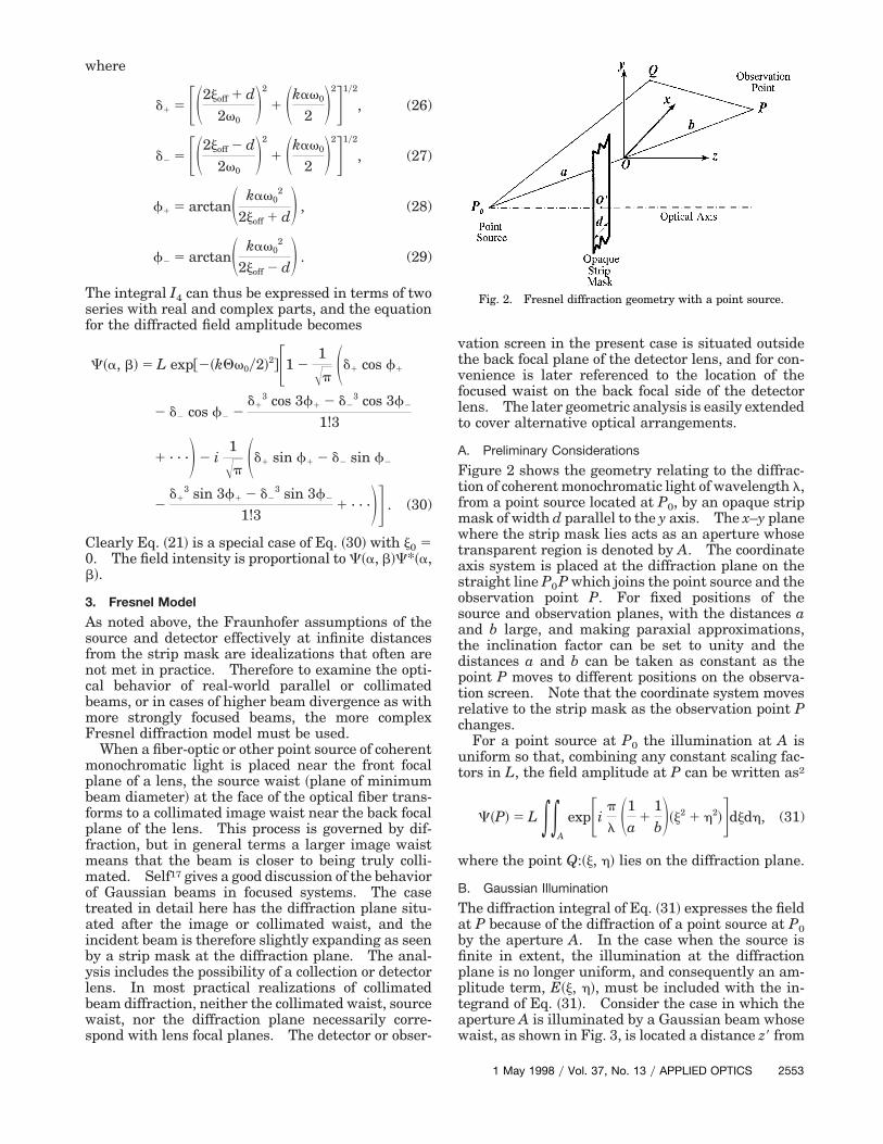
Figure 2 shows the geometry relating to the diffrac-tion of coherent monochromatic light of wavelength l,from a point source located at P0, by an opaque stripmask of width d parallel to the y axis. The x–y planewhere the strip mask lies acts as an aperture whosetransparent region is denoted by A. The coordinateaxis system is placed at the diffraction plane on thestraight line P0P which joins the point source and theobservation point P. For fixed positions of thesource and observation planes, with the distances aand b large, and making paraxial approximations,the inclination factor can be set to unity and thedistances a and b can be taken as constant as thepoint P moves to different positions on the observa-tion screen. Note that the coordinate system movesrelative to the strip mask as the observation point Pchanges.
For a point source at P0 the illumination at A isuniform so that, combining any constant scaling fac-tors in L, the field amplitude at P can be written as2
C~P! 5 L **A
expFip
l S1a
11bD~j2 1 h2!Gdjdh, (31)
where the point Q:~j, h! lies on the diffraction plane.
B. Gaussian Illumination
The diffraction integral of Eq. ~31! expresses the fieldat P because of the diffraction of a point source at P0by the aperture A. In the case when the source isfinite in extent, the illumination at the diffractionplane is no longer uniform, and consequently an am-plitude term, E~j, h!, must be included with the in-tegrand of Eq. ~31!. Consider the case in which theaperture A is illuminated by a Gaussian beam whosewaist, as shown in Fig. 3, is located a distance z9 from
Fig. 2. Fresnel diffraction geometry with a point source.
1 May 1998 y Vol. 37, No. 13 y APPLIED OPTICS 2553
25
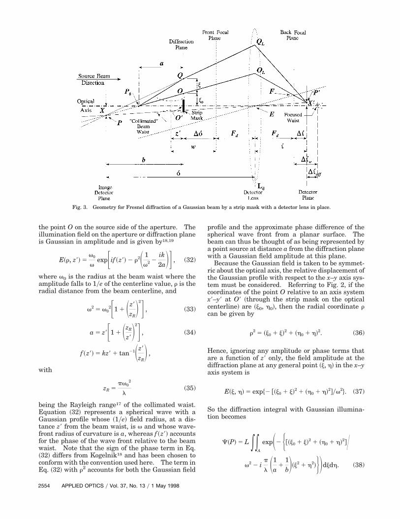
Fig. 3. Geometry for Fresnel diffraction of a Gaussian beam by a strip mask with a detector lens in place.
the point O on the source side of the aperture. Theillumination field on the aperture or diffraction planeis Gaussian in amplitude and is given by18,19
E~r, z9! 5v0
vexpFif ~z9! 2 r2S 1
v2 2ik2aDG , (32)
where v0 is the radius at the beam waist where theamplitude falls to 1ye of the centerline value, r is theradial distance from the beam centerline, and
v2 5 v02F1 1 Sz9
zRD2G , (33)
a 5 z9F1 1 SzR
z9D2G , (34)
f ~z9! 5 kz9 1 tan21Sz9
zRD ,
with
zR 5pv0
2
l(35)
being the Rayleigh range17 of the collimated waist.Equation ~32! represents a spherical wave with aGaussian profile whose ~1ye! field radius, at a dis-tance z9 from the beam waist, is v and whose wave-front radius of curvature is a, whereas f ~z9! accountsfor the phase of the wave front relative to the beamwaist. Note that the sign of the phase term in Eq.~32! differs from Kogelnik18 and has been chosen toconform with the convention used here. The term inEq. ~32! with r2 accounts for both the Gaussian field
54 APPLIED OPTICS y Vol. 37, No. 13 y 1 May 1998
profile and the approximate phase difference of thespherical wave front from a planar surface. Thebeam can thus be thought of as being represented bya point source at distance a from the diffraction planewith a Gaussian field amplitude at this plane.
Because the Gaussian field is taken to be symmet-ric about the optical axis, the relative displacement ofthe Gaussian profile with respect to the x–y axis sys-tem must be considered. Referring to Fig. 2, if thecoordinates of the point O relative to an axis systemx9–y9 at O9 ~through the strip mask on the opticalcenterline! are ~j0, h0!, then the radial coordinate rcan be given by
r2 5 ~j0 1 j!2 1 ~h0 1 h!2. (36)
Hence, ignoring any amplitude or phase terms thatare a function of z9 only, the field amplitude at thediffraction plane at any general point ~j, h! in the x–yaxis system is
E~j, h! 5 exp$2 @~j0 1 j!2 1 ~h0 1 h!2#yv2%. (37)
So the diffraction integral with Gaussian illumina-tion becomes
C~P! 5 L **A
expS2 H@~j0 1 j!2 1 ~h0 1 h!2#Yv2 2 i
p
l S1a
11bD~j2 1 h2!JDdjdh. (38)
Making the usual change of variables for Fresnelintegration,
p
2p2 5
p
l S1a
11bDj2, (39)
p
2q2 5
p
l S1a
11bDh2, (40)
then
djdh 5l
2S1a
11bD
dpdq. (41)
Noting that ~j0, h0! effectively define the observationpoint on the screen because
~x, y! 5 Sba
j0,ba
h0D , (42)
it is also possible to transform ~j0, h0! to the normal-ized observation screen coordinates P:~u, v! by
p
2u2 5
p
l S1a
11bDj0
2, (43)
p
2v2 5
p
l S1a
11bDh0
2. (44)
By including the further constant scaling factor aris-ing from Eq. ~41! in L, we can rewrite the diffractionintegral of Eq. ~38! in a normalized form as
C~u, v! 5 L * exp$2@g~v 1 q!2 2 ipq2y2#%dq
3 * exp$2@g~u 1 p!2 2 ipp2y2#%dp, (45)
where
g 5l
2v2S1a
11bD
, (46)
and the integration is understood to be taken over theaperture A.
The change of coordinates made in Eqs. ~39!, ~40!,~43!, and ~44! deals specifically with the case whenthe factor
S1a
11bD $ 0.
Below in Subsection 3.D we show that it is possible insome circumstances for this factor to be negative, andin this case it is prudent to include a minus sign in thetransform of Eqs. ~39!, ~40!, ~43!, and ~44! for thenormalized diffraction integral of Eq. ~45! to remainthe same.
C. Reduction of the Diffraction Integral
Because the two-dimensional diffraction integral ofEq. ~45! is separated with respect to p and q, it isamenable to manipulation and can be reduced to aseries solution as follows. Again making use ofBabinet’s principle,2 the double integration of Eq.~45! can be rewritten in terms of the unobstructedillumination at the diffraction plane as follows:
C~u, v! 5 L **A
5 L1 **unobstructed
aperture
2 **region of
strip mask2 . (47)
The limits on the unobstructed aperture integrationextend from 2` to ` in both directions, whereas forthe strip mask the integration extends to 6` in the qdirection, and in the p direction ~see Fig. 2 and Fig. 3!from 2~u 1 Duy2! to 2~u 2 Duy2!, where
Du2
5d2 F2
l S1a
11bDG
1y2
(48)
is the normalized strip mask half-width. The minussign arises in the p direction limits because the stripmask lies on the negative side of the x axis. If wealso now include the possibility of the strip maskbeing offset from the optical centerline by a normal-ized displacement uoff, Eq. ~47! becomes
C~u, v! 5 L *2`
`
expH2Fg~v 1 q!2 2 ip
2q2GJdq
3 S*2`
`
expH2Fg~u 1 p!2 2 ip
2p2GJdp
2 *2~u2uoff1Duy2!
2~u2uoff2Duy2!
expH2 Fg~u 1 p!2
2 ip
2p2GJdpD
; LI1~I2 2 I3!. (49)
Considering first the integrals I1 and I2 that have thesame form, we can expand the exponent in the inte-grand so that I1 can be written as7
I1 5 exp~2gv2! *2`
`
exp$2@~g 2 ipy2!q2 1 2vgq#%dq
5 exp~2gv2!S p
g 2 ipy2D1y2
expS g2v2
g 2 ipy2D. (50)
This can be rewritten by noting that
g 2 ipy2 5 5 exp~2iV!, (51)
where
V 5 tan21 p
2g, (52)
1 May 1998 y Vol. 37, No. 13 y APPLIED OPTICS 2555
5 5 gF1 1 S p
2gD2G1y2
, (53)
so that
I1 5 Îp
5expF2
g~py2g!2v2
1 1 ~py2g!2GexpHiFV
21
~py2!v2
1 1 ~py2g!2GJ .
(54)
By substituting for I1 and I2 in Eq. ~49! and againincluding the constant scaling and phase factor fromI1 in L,
C~u, v! 5 L exp~2Mv2!HÎp
5exp~2Mu2!
3 exp@i~Nu2 1 Vy2!#
2 *2U2
2U1
exp@2g~u 1 p!2# expSip
2p2DdpJ ,
(55)
where
U1 5 u 2 uoff 2 Duy2, (56)
U2 5 u 2 uoff 1 Duy2, (57)
M 5
gS p
2gD2
1 1 S p
2gD2 , (58)
N 5
Sp
2D1 1 S p
2gD2 . (59)
Because Eq. ~55! involves only one integration over arelatively short normalized region, it is in a formsuitable for numerical computation. The integral inEq. ~55! can nevertheless be reduced to a convergentseries, as shown below, leading to further simplifica-tion and, as a result, higher computation efficiency.
On expanding the brackets and completing thesquare of the exponent in the integral of Eq. ~55!, wecan write
I3 5 exp~2gu2!expS g2u2
g 2 ipy2D3 *
2U2
2U1
expF2 SÎg 2 ipy2 p 1gu
Îg 2 ipy2D2Gdp.
(60)
2556 APPLIED OPTICS y Vol. 37, No. 13 y 1 May 1998
This integral becomes more familiar with a suitablechange of coordinates by putting
z 5 Îg 2 ipy2 p 1gu
Îg 2 ipy2, (61)
so that
dz 5 Îg 2 ipy2 dp, (62)
and thus
I3 5 exp~2gu2!1
Îg 2 ipy2expS g2u2
g 2 ipy2D3 *
z2
z1
exp~2z2!dz
512 Îp
5exp~2Mu2!exp@i~Nu2 1 Vy2!#
3 @erf~z1! 2 erf~z2!#, (63)
where use has been made of Eqs. ~51!–~53! and theintegral has been written in terms of the standarderror function.16 Note that there is now a commonfactor between I2 and I3. The integral limits comedirectly from Eq. ~61! and are
z1 5 Îg 2 ipy2 U1 1gu
Îg 2 ipy2, (64)
z2 5 Îg 2 ipy2 U2 1gu
Îg 2 ipy2. (65)
For the moment just considering z1, Eqs. ~51!–~53!can be used to recast this as
z1 5 2 Î5 ~cos Vy2 2 i sin Vy2!U1
1gu
Î5~cos Vy2 1 i sin Vy2!,
5 S gu
Î52 Î5 U1Dcos Vy2
1 iS gu
Î51 Î5 U1Dsin Vy2,
; s1~cos F1 1 i sin F1!, (66)
where
F1 5 tan21F~gu 1 5U1!tan Vy2gu 2 5U1
G , (67)
s1 5 HFS gu
Î52 Î5 U1Dcos Vy2G2
1 FS gu
Î51 Î5 U1Dsin Vy2G2J1y2
5 Sg2u2
52 2guU1 cos V 1 5U1
2D1y2
. (68)
Similarly
z2 ; s2~cos F2 1 i sin F2!, (69)
where
F2 5 tan21F~gu 1 5U2!tan Vy2gu 2 5U2
G , (70)
s2 5 Sg2u2
52 2guU2 cos V 1 5U2
2D1y2
. (71)
The error function can be expressed in terms of aseries expansion as16
erf~z! 52
ÎpSz 2
z3
1!31
z5
2!52
z7
3!71 · · ·D . (72)
Thus with use of Eqs. ~63!, ~66!, ~69!, and ~72! inconjunction with de Moivre’s theorem and lumpingthe constant amplitude and phase factor of C with L,the diffracted field of Eq. ~55! becomes
C~u, v! 5 L exp@2M~u2 1 v2!#F1 21
ÎpSs1 cos F1
2 s2 cos F2 2s1
3 cos 3F1 2 s23 cos 3F2
1!3
1 · · ·D2 i1
ÎpSs1 sin F1 2 s2 sin F2
2s1
3 sin 3F1 2 s23 sin 3F2
1!31 · · ·DG . (73)
The intensity at any normalized screen position isagain proportional to the product of the field and itscomplex conjugate C~u, v!C*~u, v!.
D. Gaussian–Fresnel Geometry
When the diffraction plane does not coincide with thewaist of the collimated beam or the detector plane isnot at the back focal plane of the detector lens, thesource illumination and detector are no longer effec-tively at infinity. To determine appropriate dis-tances of source to diffraction plane spacing anddiffraction plane to screen spacing, the system mustbe analyzed with the detector lens in place with suit-able geometry. Figure 3 shows the geometry forFresnel diffraction ~in the x–z plane only! with thediffraction plane in the expanding part of the colli-mated beam and with a detector lens Ld in place.The detector is placed a total distance Dı from theback focal plane of Ld, which is comprised of Dıw, thedistance of the ~unobscured! focused beam waist fromthe lens back focal plane and Dıoff, an additional offsetof the detector from the waist. Note that Dıoff istaken as positive for displacements away from thedetector lens.
For the sake of simplicity, the geometry shown inFig. 3 and the derivation that follows is only in onedimension but the argument is easily extended to theother direction where appropriate. The waist of the
collimated beam is a distance w from the detectorlens front focal plane, whereas the strip mask at thediffraction plane is a distance Do from the detectorlens front focal plane. The strip mask has infiniteextent into the page of Fig. 3. As outlined above andshown in Fig. 3, the illumination of the Gaussianbeam on the diffraction plane is effectively repre-sented by a point source at P0 whose distance a fromthe diffraction plane is given by Eq. ~34! and whosefield at the diffraction plane is Gaussian and given bythe amplitude of Eq. ~32!. In the usual constructionfor Fresnel geometry ~see above and Refs. 1 and 2!,light from the point source illuminates each point onthe diffraction plane, each of which in turn acts as asource of secondary wavelets that recombine to formthe field at the observation point on the screen ordetector. With a detector lens in place, the distanceb from the diffraction plane to what is effectively afictitious image detector plane must be establishedwith the help of geometrical optics from the construc-tion in Fig. 3.
To produce Fig. 3 the procedure is as follows. Con-sider a general observation point on the plane of thedetector that is a distance X9 from the optical axis.To determine the path of the straight through orreference ray P0OOL after refraction by the thin lensLd, observe that a fictitious ray EF, drawn parallel toP0OOL but passing through the center of the lens Ldat E, must intersect the refracted ray OLP9 on theback focal plane of the lens at F. Each point P9 onthe detector is thus intimately linked to each point Oat the diffraction plane @see Eq. ~42!#. Note also thatthe point P9 on the detector has an associated realinverted image point P on the front focal side of thelens whose position can be found easily by drawingtwo more fictitious rays. A ray P9E passes undi-verted through the center of the lens while a ray thatis the extension P0OOL will intersect P9E at the im-age point P. The point P now effectively forms theobservation point to be used in the derivation of dis-tances in the Fresnel treatment. The path taken byany general ray P0Q after leaving the diffractionplane is found by noting that the ray QQL must ap-pear to come from the image point P if it also is topass through the detector observation point P9.Note that if the detector plane and consequently thepoint P9 were on the lens side of the back focal plane~Dı , 0!, the point P would appear on the detector sideof the lens and transform to a virtual upright imageof P9.
Because the chief property of the lens is to alter thewave-front radius of curvature, the phase differencesof rays leaving typical points Q relative to that fromO are fully accounted for by taking the distance PO asequal to b in the Fresnel geometry. As previouslynoted with paraxial rays, there is no loss of generalityby taking this distance as constant and equal to itsprojection on the optical axis. It is important to notethat, in the particular case examined in Fig. 2, thepoint P lies on the source side of the diffraction planeand consequently the path length through P0Q is nowshorter than the straight through path by way of
1 May 1998 y Vol. 37, No. 13 y APPLIED OPTICS 2557
P0O. In this case we must therefore take b to benegative. Various parameters can now be deter-mined, in particular b, in terms of the prescribedsystem geometry as outlined below.
For the purposes of what follows it is convenient torefer to the point P as the object and to the point P9 asthe image of this object because this is what wouldnormally be expected on the basis of the direction ofthe light rays. With use of the usual convention theobject and image distances, o and ı, respectively, aretaken from the center of the thin lens as shown in Fig.3 and are related by1
1o
11ı
51Fd
,
hence
o 5Fdı
ı 2 Fd,
5FdıDı
, (74)
5Fd
2
Dı1 Fd (75)
with use of Dı 5 ı 2 Fd. Here Fd is the detector lensfocal length. From similar triangles the effectivemagnification between the image detector plane andthe true detector plane is given by
XX9
5oı
,
5Fd
Dı, (76)
where X is now the distance of the point P from theoptical axis and substitution has been made from Eq.~74!. Similarly, the magnification in the y direction~into the page of Fig. 3, but not shown! will be iden-tical, and hence
YY9
5Fd
Dı. (77)
On inspection of Fig. 3 and with use of Eq. ~73! it canbe deduced that
b 5 Do 2Fd
2
Dı, (78)
where Do is the known distance of the diffractionplane from the lens front focal plane and the sign ofb in the present case has been chosen as negative.The pole at Dı 5 0 effectively puts the observationplane at infinity and corresponds to the Fraunhofercondition for the detector. Equation ~78! can be usedunambiguously provided Dı is taken as positive awayfrom the detector lens.
As noted above, the parameter a comes directlyfrom Eq. ~34!, although in the case of a converging
2558 APPLIED OPTICS y Vol. 37, No. 13 y 1 May 1998
beam on the diffraction plane, a will be negative so asto properly account for the relative phase differenceof rays reaching the diffraction plane. It is also con-venient to introduce the distance w of the collimatedwaist from the lens front focal plane where
w 5 z9 1 Do. (79)
When performing experiments it can be convenient tolocate the detector plane with respect to the unob-structed focused spot on the back focal side of thelens, as this may be easier to accurately locate thanthe lens back focal plane itself. As the collimatedwaist is distant w 1 Fd from the center of lens Ld, andthe focused waist is Dıw 1 Fd from the lens center onthe other side, the distance of the focused waist, onthe back focal side, from the back focal plane of thelens is17
Dıw
Fd5
wFd
SwFdD2
1 SzR
FdD2 , (80)
where the collimated side Rayleigh range zR is givenby Eq. ~35!. Any additional offset Dıoff of the detectorfrom this focused waist position must be added in toobtain the full detector displacement as
Dı 5 Dıw 1 Dıoff. (81)
4. Computational Technique
It is evident from Eqs. ~21!, ~30!, and ~73! that, tocalculate the field at any point on a detector, suffi-cient terms of the series must be summed until ade-quate convergence is obtained. To avoid prematureseries truncation, at larger values of d it is necessaryto use a secondary convergence test. A simplescheme is to examine the gradient of the nth termversus the n plot by checking the magnitude of thedifference between adjacent terms against a fractionof the partial-sum magnitude. Generally only10–20 terms are needed for sufficient convergence ofthe series. Note that care must be taken to ensurethat calculation of the angles in Eqs. ~28!, ~29!, ~67!,and ~70! puts them in the correct quadrants.
For large-width masks andyor observation pointsfar from the optical centerline, the magnitude of theterms in the series of Eq. ~73! become extremely largeprior to adequate convergence. This can lead to aloss of precision in the ~computer-stored! series termsand partial sum and result in the series erroneouslydiverging. This problem can be overcome by the useof an asymptotic expansion for erf~z!, for large valuesof z, in place of the Maclaurin expansion of Eq. ~72!.Note that the field obtained by Eq. ~55! does not sufferfrom this convergence problem and can alternativelybe used to calculate intensities in which the seriessolution is problematic. The integral in Eq. ~55! isthe vector form of a modified Fresnel integral8 whosetwo-component integrand comprises amplitude-modulated trigonometric functions of rapidly increas-
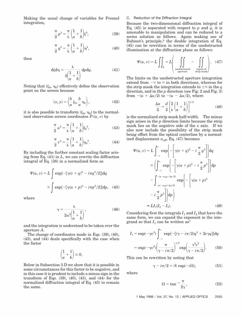
Fig. 4. Schematic diagram of the Fraunhofer diffraction experimental arrangement.
ing frequency and generally rapidly decreasingamplitude as p increases in magnitude. Because thewavelength of the integrand changes rapidly, the nu-merical integration should be performed one wave-length at a time taking care in choosing values of p asit changes sign. Intensity computed by use of theseries solution of Eq. ~73! is approximately 50% fasterthan the numerical integration of Eq. ~55!.
5. Experimental Technique
Shown schematically in Fig. 4 is the experimentalsetup used to verify the Fraunhofer model. A 2-mWunpolarized He–Ne laser ~l 5 633 nm!, whose nom-inal 1ye2 intensity diameter on the front resonatormirror is 490 mm, is spatially filtered by two low-power ~F 5 35.7 mm! microscope objectives strad-dling a 100-mm-diameter pinhole. Collimation atthe sample or diffraction plane is established by firstobserving the back reflected light from a mirrorplaced at the diffraction plane. A beam splitter ~notshown! inserted between the laser and first objectiveallows the reflected spatially filtered pattern emerg-ing from the pinhole to be optimized. As an addi-tional quick check for location of the collimated beamwaist, a 10-mm apertured silicon photodiode detectorwas used to probe the beam centerline intensity atvarious axial positions to locate a stationary pointwhose uncertainty was approximately 63 mm axi-ally. The measured 1ye2 diameter of the collimatedbeam was 337.6 mm ~see below!.
Wire samples are mounted on an XYZ stage to allowprecise lateral positioning of the wires on the beamcenterline. The two wires used here are made fromdrawn NiCr and have projection microscope-measureddiameters of 152.3 and 199.2 mm. The diffractionpatterns from the sample wires are monitored in thefar field by laterally scanning a 10-mm apertured sili-con photodiode detector perpendicular to the axis ofthe wires. The detector is also mounted on top of amanual XYZ stage to allow precise positioning withinthe beam. The detector pinhole is 1.5 m from thediffraction plane. The detector signal is amplifiedand low-pass filtered prior to being sent by differentiallines to an analog-to-digital board in a personal com-puter. The motorized translation stage is dc motordriven and has a positioning resolution of ;0.1 mm.Data are logged by the computer at a selected numberof stations throughout a traverse with a pause of 200ms prior to taking the measurement to allow any vi-brations to die out.
Precise lateral positioning of the wires on the beamcenterline is important, as offsets as small as a fewmicrometers can result in significant asymmetry inthe diffraction patterns. The following techniquewas used to center the wires in the beam. The10-mm detector aperture was temporarily replaced bya 2-mm-diameter aperture so as to capture approxi-mately 70% of the far-field beam diameter and cen-tered in the beam by observing the peak in thedetector signal. The mounted wire sample was thenpositioned laterally to achieve maximum beam occlu-sion by minimizing the observed detector signal.Care was also taken to ensure that the diffractionpatterns were in line with the traverse direction.The 10-mm aperture was then replaced and centeredin the main lobe of the diffraction pattern.
For verification of the Fresnel model, the barebeam emerging from the laser was used to illuminatethe sample wires approximately 100 mm from thefront of the laser casing. The Rayleigh range~pv0
2yl! of this beam is 298 mm, which puts thediffraction plane ~z9 ; 150 mm! in a region of signif-icant wave-front curvature. The measured 1ye2 di-ameter of the beam at the diffraction plane for thesemeasurements was 520.0 mm. For these measure-ments the detector was positioned 1.4 m from thewire samples.
6. Results and Discussion
A. Fraunhofer Measurements
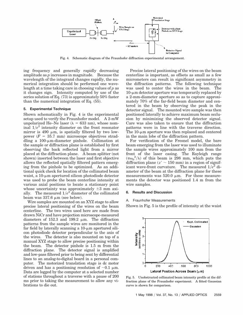
Shown in Fig. 5 is the profile of intensity at the waist
Fig. 5. Unobstructed collimated beam intensity profile at the dif-fraction plane of the Fraunhofer experiment. A fitted Gaussiancurve is shown for comparison.
1 May 1998 y Vol. 37, No. 13 y APPLIED OPTICS 2559
of the collimated beam with a fitted Gaussian curvefor comparison. Although the measured beam pro-file is essentially Gaussian in shape, some deviationincluding asymmetry is apparent. The 1ye2 beamdiameter of 376.6 mm was found from the raw dataafter correcting for zero offset. Beam diameters de-termined in this manner were generally within ap-proximately 5% of the values determined from aGaussian fit. Measurement of the beam diameter ata number of far-field axial stations allowed the diver-gence half-angle of 1.18 3 1023 rad to be deduced.This is in good agreement with the far-field diver-gence half-angle of ~lypv0! 1.19 3 1023 rad based onthe measured beam size at the waist.
Figure 6 shows the measured and predicted Fraun-hofer diffraction pattern from the 152.3-mm wire.The measured curve generally shows good symmetryalthough a wobble is evident in the main right sidelobe. The theoretical and experimental curves werematched by normalizing the respective peak intensi-ties to unoccluded intensities on the beam centerline.Some differences in height are apparent but the over-all shape as well as fringe location of the theoreticalcurve is in fairly good agreement with the measureddata. Some differences are to be expected on thebasis of a non-Gaussian beam profile, deviations fromwave-front flatness at the diffraction plane, error inwire diameter measurement and wire cleanliness,
Fig. 6. Measured and predicted Fraunhofer diffraction patternfrom the 152.3-mm wire.
Fig. 7. Measured and predicted Fraunhofer diffraction patternfrom the 199.2-mm wire.
2560 APPLIED OPTICS y Vol. 37, No. 13 y 1 May 1998
possible surface roughness effects,20 and approxima-tions involved in the use of a scalar model.21 Figure7 shows the measured and predicted Fraunhofer dif-fraction patterns for the 199.2-mm wire. Generalagreement of the two curves is again reasonably good.
B. Fresnel Measurements
The intensity profile of the bare laser beam 100 mmfrom the front of the laser casing is shown in Fig. 8along with a fitted Gaussian curve for comparison.The measured beam profile is essentially Gaussian inshape but again some deviation including asymmetryis apparent. The 1ye2 beam diameter was found tobe 520.0 mm. Measurement of the beam diameter ata number of far-field axial stations gave the diver-gence half-angle as 8.19 3 1024 rad. This is in goodagreement with the far-field divergence half-angle of8.22 3 1024 rad based on the manufacturer’s nominalbeam size at the waist.
Figure 9 shows the measured and predictedFresnel diffraction patterns for the 152.3-mm wire.Peak intensities of the experimental and theoreticaldata have again been normalized by their respectiveunobstructed beam centerline values. The mea-sured curve shows a little asymmetry, and the firstside-lobe minima no longer come down to zero. Al-though the theory underestimates the intensity in
Fig. 8. Unobstructed beam intensity profile at the diffractionplane of the Fresnel experiment 100 mm from the laser casing. Afitted Gaussian curve is shown for comparison.
the first side lobes, the overall shape as well as fringelocation of the theoretical curve is in good agreementwith the measured data. The theoretical data weregenerated by use of the measured diffraction planebeam size in conjunction with the nominal waistbeam size to infer z9 from Eq. ~33! and hence wave-front radius of curvature a from Eq. ~34!. The mea-sured and predicted Fresnel diffraction patterns forthe 199.2-mm wire are shown in Fig. 10. Good gen-eral agreement is again evident.
These demonstrations with the beam 100 mm outfrom the front of the laser highlight the need forparticular care if a reasonable approximation toFraunhofer conditions is to be established. Condi-tions that are not fully Fraunhofer result particularlyin sensitivity of the diffraction patterns to asymmetrywith off-center wires and modification of the firstside-lobe structure.
7. Conclusions
Two-dimensional Fraunhofer and Fresnel diffractionmodels have been used to develop rapidly convergentseries solutions to the problem of diffraction of aGaussian beam by an opaque strip mask. The mod-els have utility in the diffraction of laser beamsaround wires and fibers. Measurements made withwires under both Fraunhofer and Fresnel conditionsshow good agreement with theoretical predictions.The demonstrations here with small-diameter beamsemphasize the need for care if a reasonable approxi-mation to Fraunhofer conditions is to be established.
Appendix A. Nomenclature
A Transparent region of the plane or aperturewhere the strip mask lies.
d Width of strip mask.Fd Focal length of focusing lens at the detector.
i =21I1, I2, . . . Integrals to be evaluated.
J0 Zero-order Bessel function of the first kind.L Lumped constant of the diffraction integral.k Wave number 2pyl.
M A system-dependent constant.N A system-dependent constant.
u Normalized displacement.uoff Normalized ~Fresnel! mask offset from beam
centerline.u1, u2 Normalized complex limits of integration for I4.
x, y Coordinates of a point on the detector plane.z Coordinate axis along the optical centerline.
z9 Distance of diffraction plane from beam waist.a, b Direction angles of the diffracted light.
g A system-dependent constant.d, d1, d2 Amplitude for computation of Fraunhofer se-
ries sum.z A dummy variable.
Q Angle of diffracted light with respect to z axis.l Wavelength of laser light.
joff Displacement of strip mask from h axis tobeam centerline.
j, h Coordinates of a point on the diffraction plane.r Radial coordinate on ~j, h! plane.
s, s1, s2 Amplitude for computation of Fresnel seriessum.
f, f1, f2 Angle for computation of Fraunhofer seriessum.
F1, F2 Angle for computation of Fresnel series sum.C~a, b! Diffracted field amplitude.
C*~a, b! Complex conjugate of diffracted field ampli-tude.
C9~j, h! Field of illumination at the diffraction plane.C0 Centerline field strength.
v 1ye field amplitude or 1ye2 intensity radius ofGaussian beam.
v0 1ye field amplitude or 1ye2 intensity radius ofGaussian beam waist.
The author thanks Duncan Butler for his helpfulreview of this manuscript. Support for this researchwas provided by Australian Woolgrowers and theAustralian government through the InternationalWool Secretariat and the Commonwealth Scientificand Industrial Research Organisation.
References1. E. Hecht and A. Zajac, Optics ~Addison-Wesley, New York,
1974!.2. M. Born and E. Wolf, Principles of Optics ~Pergamon, New
York, 1980!.3. T. W. Mayes and B. F. Melton, “Fraunhofer diffraction of vis-
ible light by a narrow slit,” Am. J. Phys. 62, 397–403 ~1994!.4. H. C. van de Hulst, The Scattering of Light by Small Particles
~Dover, New York, 1981!.5. F. Kuik, F. F. de Haan, and J. W. Hovenier, “Single scattering of
light by circular cylinders,” Appl. Opt. 33, 4906–4918 ~1994!.6. R. T. Wang and H. C. van de Hulst, “Application of the exact
solution for scattering by an infinite cylinder to the estimationof scattering by a finite cylinder,” Appl. Opt. 34, 2811–2821~1995!.
7. A. W. Snyder and J. D. Love, Optical Waveguide Theory ~Chap-man & Hall, London, 1983!.
8. M. Glass, T. P. Dabbs, and P. W. Chudleigh, “The optics of thewool Fiber Diameter Analyser,” Text. Res. J. 65~2!, 85–94~1995!.
9. M. Glass, “Fresnel diffraction from curved fiber snippets withapplication to fiber diameter measurement,” Appl. Opt. 35,1605–1616 ~1996!.
10. D. Lebrun, S. Belaid, C. Ozkul, K. F. Ren, and G. Grehan,“Enhancement of wire diameter measurements: comparison
1 May 1998 y Vol. 37, No. 13 y APPLIED OPTICS 2561
between Fraunhofer diffraction and Lorenz-Mie theory,” Opt.Eng. 35, 946–950 ~1996!.
11. H. Wang and R. Valdivia-Hernandez, “Laser scanner and dif-fraction pattern detection: a novel concept for dynamic gaug-ing of fine wires,” Meas. Sci. Technol. 6, 452–457 ~1995!.
12. S. Kozaki, “Scattering of a Gaussian beam by a homogeneousdielectric cylinder,” J. Appl. Phys. 53, 7195–7200 ~1982!.
13. E. Zimmermann, R. Dandliker, and N. Souli, “Scattering of anoff-axis Gaussian beam by a dielectric cylinder compared witha rigorous electromagnetic approach,” J. Opt. Soc. Am. A 12,398–403 ~1995!.
14. J. E. Pearson, T. C. McGill, S. Curtain, and A. Yariv, “Diffrac-tion of Gaussian laser beams by a semi-infinite plane,” J. Opt.Soc. Am. 59, 1440–1445 ~1969!.
15. H. T. Yura and T. S. Rose, “Gaussian beam transfer throughhard-aperture optics,” Appl. Opt. 34, 6826–6828 ~1995!.
2562 APPLIED OPTICS y Vol. 37, No. 13 y 1 May 1998
16. E. Kreyszig, Advanced Engineering Mathematics ~Wiley, NewYork, 1983!.
17. S. A. Self, “Focusing of spherical Gaussian beams,” Appl. Opt.22, 658–661 ~1983!.
18. H. Kogelnik, “On the propagation of Gaussian beams of lightthrough lenslike media including those with a loss or gainvariation,” Appl. Opt. 4, 1562–1569 ~1965!.
19. W. H. Carter, “Focal shift and concept of effective Fresnelnumber for a Gaussian laser beam,” Appl. Opt. 21, 1989–1994~1982!.
20. P. Rochon, T. J. Racey, and N. Gauthier, “Diffraction fromsmall wires, including surface roughness,” Opt. Acta. 31,1385–1397 ~1984!.
21. R. G. Greenler, J. W. Hable, and P. O. Slane, “Diffractionaround a fine wire: how good is the single-slit approxima-tion?” Am. J. Phys. 58, 330–331 ~1990!.