Entropy 2011, 13, 1380-1402; doi:10.3390/e13071380 OPEN ACCESS entropy ISSN 1099-4300 www.mdpi.com/journal/entropy Article Diffuser and Nozzle Design Optimization by Entropy Generation Minimization Bastian Schmandt and Heinz Herwig Institute of Thermo-Fluid Dynamics, Hamburg University of Technology, Denickestr. 17, 21073 Hamburg, Germany; E-Mail: [email protected]Author to whom correspondence should be addressed; E-Mail: [email protected]; Tel.: +49-(0)-40-42878-3268; Fax: +49-(0)-40-42878-2967. Received: 10 June 2011; in revised form: 1 July 2011 / Accepted: 15 July 2011 / Published: 20 July 2011 Abstract: Diffusers and nozzles within a flow system are optimized with respect to their wall shapes for a given change in cross sections. The optimization target is a low value of the head loss coefficient K, which can be linked to the overall entropy generation due to the conduit component. First, a polynomial shape of the wall with two degrees of freedom is assumed. As a second approach six equally spaced diameters in a diffuser are determined by a genetic algorithm such that the entropy generation and thus the head loss is minimized. It turns out that a visualization of cross section averaged entropy generation rates along the flow path should be used to identify sources of high entropy generation before and during the optimization. Thus it will be possible to decide whether a given parametric representation of a component’s shape only leads to a redistribution of losses or (in the most-favored case) to minimal values for K. Keywords: second law analysis; entropy generation; optimization; diffuser 1. Introduction Diffusers and nozzles may either be the last part of a flow system, releasing the fluid into the ambient, or a conduit component within a flow system. These are two very different situations and as a consequence optimization occurs with respect to different aspects. The main purpose of using an
Diffuser and Nozzle Design Optimization by Entropy GenerationMinimizationBastian Schmandt � and Heinz Herwig
Institute of Thermo-Fluid Dynamics, Hamburg University of Technology, Denickestr. 17,21073 Hamburg, Germany; E-Mail: [email protected]
� Author to whom correspondence should be addressed; E-Mail: [email protected];Tel.: +49-(0)-40-42878-3268; Fax: +49-(0)-40-42878-2967.
Received: 10 June 2011; in revised form: 1 July 2011 / Accepted: 15 July 2011 /Published: 20 July 2011
Abstract: Diffusers and nozzles within a flow system are optimized with respect to theirwall shapes for a given change in cross sections. The optimization target is a low value ofthe head loss coefficientK, which can be linked to the overall entropy generation due to theconduit component. First, a polynomial shape of the wall with two degrees of freedom isassumed. As a second approach six equally spaced diameters in a diffuser are determinedby a genetic algorithm such that the entropy generation and thus the head loss is minimized.It turns out that a visualization of cross section averaged entropy generation rates along theflow path should be used to identify sources of high entropy generation before and during theoptimization. Thus it will be possible to decide whether a given parametric representation ofa component’s shape only leads to a redistribution of losses or (in the most-favored case) tominimal values forK.
Keywords: second law analysis; entropy generation; optimization; diffuser
1. Introduction
Diffusers and nozzles may either be the last part of a flow system, releasing the fluid into theambient, or a conduit component within a flow system. These are two very different situations andas a consequence optimization occurs with respect to different aspects. The main purpose of using an
Entropy 2011, 13 1381
end diffuser may be a high pressure recovery, while for a nozzle, however, it may be the homogeneity ofthe velocity profile, as for example with a nozzle in an open wind tunnel.When diffusers and nozzles are internal conduit components within a flow system, their purpose is to
increase or decrease the flow cross sections as shown in Figure 1. On a length L the hydraulic diameterchanges from Dhu to Dhd with the indices u and d for upstream and downstream. Then the otherwisefully developed flow is influenced by the components within an upstream and downstream length Lu andLd, respectively.
With Dhu, Dhd and L prescribed, the open question is which shape of the wall (different from thestraight walls in Figure 1) will be the best. Here “best” means what can result in the least loss of totalhead due to the presence of the diffuser or nozzle.This is the situation analyzed here: How to find the optimum conduit design by varying the wall
shape of an internal diffuser or nozzle with prescribed values of Dhu, Dhd and L for a certain Reynoldsnumber of the flow. The optimization target is to minimize the head loss coefficient with a value as lowas possible. The main purpose, however, is not only to provide the information about the best diffuseror nozzle design but also to introduce a method for a systematic optimization based on the least entropygeneration in the flow field.
2. Head Loss, Dissipation and Entropy Generation
Diffusers and nozzles, used as internal flow system components, are characterized by their head losscoefficient K. This coefficient describes the conversion of mechanical energy to thermal energy by adissipation process.A reasonable definition ofK therefore is
K ≡ϕ
u2m/2
(1)
with ϕ as specific dissipation due to the presence of the conduit component in the flow system.
Entropy 2011, 13 1382
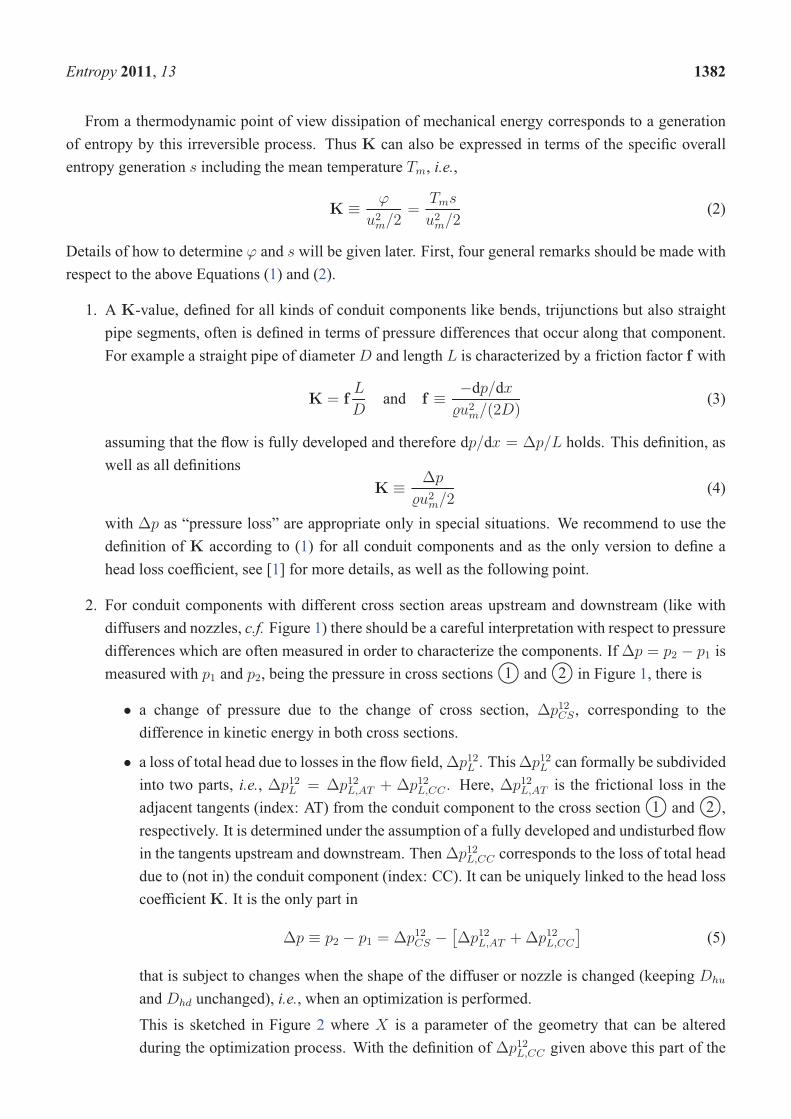
From a thermodynamic point of view dissipation of mechanical energy corresponds to a generationof entropy by this irreversible process. Thus K can also be expressed in terms of the specific overallentropy generation s including the mean temperature Tm, i.e.,
K ≡ϕ
u2m/2
=Tms
u2m/2
(2)
Details of how to determine ϕ and s will be given later. First, four general remarks should be made withrespect to the above Equations (1) and (2).
1. A K-value, defined for all kinds of conduit components like bends, trijunctions but also straightpipe segments, often is defined in terms of pressure differences that occur along that component.For example a straight pipe of diameterD and length L is characterized by a friction factor f with
K = fL
Dand f ≡
−dp/dx�u2
m/(2D)(3)
assuming that the flow is fully developed and therefore dp/dx = Δp/L holds. This definition, aswell as all definitions
K ≡Δp
�u2m/2
(4)
with Δp as “pressure loss” are appropriate only in special situations. We recommend to use thedefinition of K according to (1) for all conduit components and as the only version to define ahead loss coefficient, see [1] for more details, as well as the following point.
that is subject to changes when the shape of the diffuser or nozzle is changed (keeping Dhu
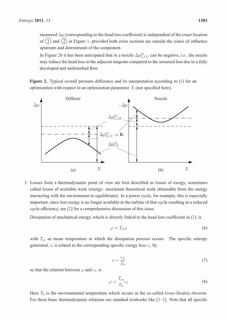
and Dhd unchanged), i.e., when an optimization is performed.This is sketched in Figure 2 where X is a parameter of the geometry that can be alteredduring the optimization process. With the definition of Δp12L,CC given above this part of the
Figure 2. Typical overall pressure difference and its interpretation according to (5) for anoptimization with respect to an optimization parameter X (not specified here).
Diffuser Nozzle
X X(a) (b)
Δp −Δp
Δp12CS
Δp12L,CC ∝ K
Δp12L,AT
3. Losses from a thermodynamic point of view are best described as losses of exergy, sometimescalled losses of available work (exergy: maximum theoretical work obtainable from the energyinteracting with the environment to equilibrium). In a power cycle, for example, this is especiallyimportant, since lost exergy is no longer available in the turbine of that cycle resulting in a reducedcycle efficiency, see [2] for a comprehensive discussion of this issue.
Dissipation of mechanical energy, which is directly linked to the head loss coefficient in (2), is
ϕ = Tms (6)
with Tm as mean temperature at which the dissipation process occurs. The specific entropygenerated, s, is related to the corresponding specific exergy loss eL by
s =eLT0
(7)
so that the relation between ϕ and eL is
ϕ =Tm
T0
eL (8)
Here T0 is the environmental temperature which occurs in the so-called Gouy-Stodola theorem.For these basic thermodynamic relations see standard textbooks like [3–5]. Note that all specific
Entropy 2011, 13 1384
values introduced so far (ϕ, s, eL) are their absolute values referred to the mass or more convenientfor an interpretation their absolute values per time, i.e., rates Φ, S, EL, referred to the mass flux min the flow system.
Since according to (8) it depends on the temperature level Tm how much exergy is lost with acertain dissipation the head loss coefficient K defined in (1) is not a general measure for theexergy lost in a conduit component.
Hence, in addition to K a second coefficient called exergy loss coefficient should be introduced.WithKE defined as
KE ≡
eLu2m/2
=T0s
u2m/2
(9)
there now are two loss coefficientsK andKE related to each other by
K =Tm
T0
KE (10)
If, for example, the head loss occurs in a power cycle at an upper temperature level Tm, thetemperature ratio may be Tm/T0 = 3. Thus, the exergy loss is only one third of what it would beif the same flow would have the ambient temperature T0 instead of Tm.
4. During the optimization process described hereafter, K-values of the diffusers and nozzles willhave to be determined. According to (2) this can either be done by the determination of ϕ(dissipation rate per mass flux) or of s (entropy generation rate per mass flux). We definitely prefers since it is the more fundamental quantity of the conversion process (mechanical → thermalenergy). A further argument in favor of the specific entropy is that then a common quantity existswhen also losses (of exergy) in a superimposed heat transfer process are accounted for, see [1] formore details of this convective heat transfer situation.
3. Review of Literature
The scope of this paper is to provide a method for the design optimization of conduit componentslike diffusers and nozzles, based on the head losses involved. As shown in the previous section this canbe accomplished by determining the entropy generation. Since s is closely related to the second law ofthermodynamics this method is called second law analysis (SLA). A literature review with respect tothis special aspect should, however, be accompanied by references about entropy in general.
3.1. Literature about Entropy in General
There is a vast amount of textbooks and monographs about thermodynamics which all have majorparts with respect to entropy in it. Special books about entropy range from easy to read introductionslike [6–8] over more comprehensive books like [9] to very challenging ones like [10,11].
3.2. Literature about Entropy Generation
The SLA approach in which irreversibilities are identified and determined is described and applied infundamental studies like [12–14], for example.
Entropy 2011, 13 1385
Almost all studies that incorporate a second law analysis refer to one of the several importantcontributions by Adrian Bejan, see [12,15–17]. In these studies entropy generation is often determinedas an integral value within a finite solution domain, either by global balances or by integration of thelocal entropy generation density. A general and systematic comparison of various approaches can befound in [18,19].In general, one can analyze a system as a whole or have a closer look to single components within a
complex system. Studies about whole systems like [20–22] aim at improving the system performance,though there is no systematic optimization strategy involved, like in the special study [23], for example.Detailed studies about single components can be found in [24], where a vortex tube is analyzed, in [25]with a study about a crossflow heat exchanger, or in [26] where rectangular ducts are investigated, justto mention a few typical investigations out of the big number of studies based on the SLA approach.
where cp is optimized using the standard k − ε turbulence model with wall functions and a similarparameterization as discussed here for the wall shape. In [27] the so-called Response SurfaceApproximation of cp based on a relatively small number of model evaluations is used as a surrogatefor repetitive model evaluations during a conventional search strategy. Different from [27], a geneticalgorithm is used in [28] in order to test a large variety of polynomial wall parameterizations.An extensive overview about optimization in research and industrial relevant applications using CFD
is given in [29], where various optimization methods are explained together with illustrative examples.Especially the adjoint method is discussed in detail.
4. Entropy Generation as an Optimization Criterion
For diffusers and nozzles, dissipation and therefore the entropy generation due to this process is thecrucial quantity that should be optimized, i.e., minimized in the situation under consideration. Beforea strategy with respect to this optimization will be discussed in the next section, we first show in detailhow the overall entropy generation due to the components can be determined.
Entropy 2011, 13 1386
4.1. Determination of the Overall Entropy Generation Rate
As indicated in Figure 1 already, the conduit component has an influence on the upstream anddownstream flow, so that corresponding lengths Lu and Ld have been introduced. Within these lengthsthe influence of the component can be felt by the otherwise fully developed and undisturbed flow. Inorder to have a clearly defined length of influence upstream and downstream, related lengths Ld and Lu
are introduced. They are defined as those lengths up to which 95% of the overall upstream or downstreaminfluence occurs and are explained in more details later.Altogether the situation sketched in Figure 3 appears: A part of the flow field, Vc, being the interior of
the conduit component and upstream as well as downstream parts of it, Vu and Vd, have to be analyzedwith respect to the (additional) entropy generation due to the component.
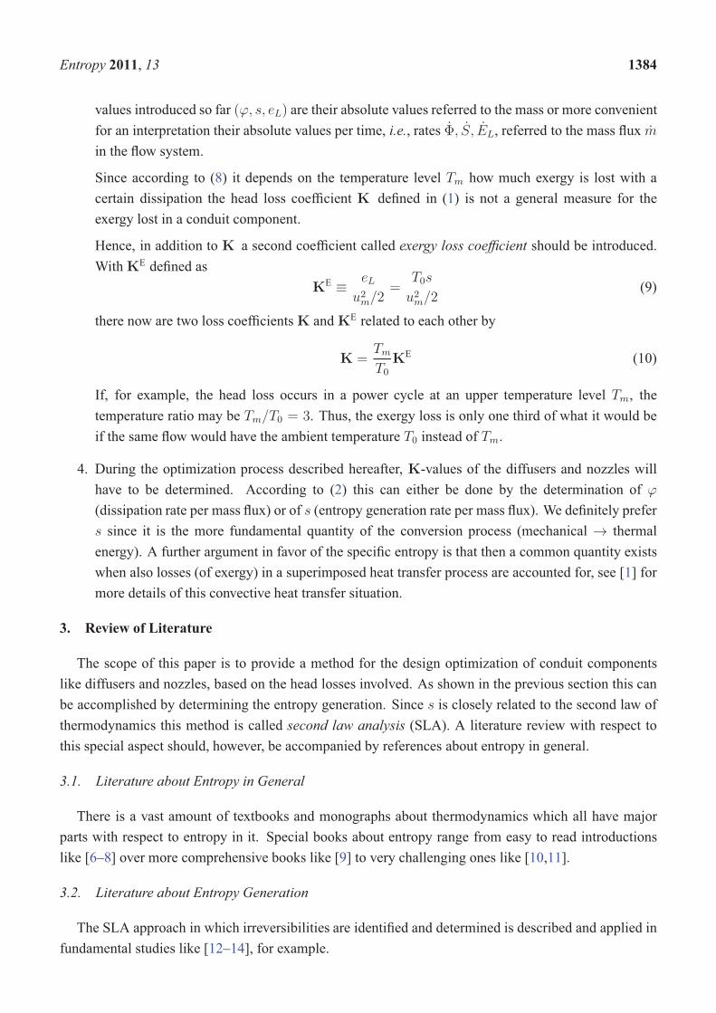
Figure 3. Different parts of the flow field determined or influenced by the conduitcomponent. Vc: volume of the component itself; Vu: upstream volume affected by thecomponent; Vd: downstream volume affected by the component.
Vc
conduitcomponent
upstream channel part Vu downstream channel part VdLu Ld
This entropy generation happens locally due to velocity gradients under the action of a finite molecularviscosity μ. Its amount, see [5] for example, in Cartesian coordinates is:
S ′′′ =μ
Tm
(2
[(∂u
∂x
)2
+
(∂v
∂y
)2
+
(∂w
∂z
)2]
+
(∂u
∂y+
∂v
∂x
)2
+
(∂u
∂z+
∂w
∂x
)2
+
(∂v
∂z+
∂w
∂y
)2)
(11)
This local value (with unitsW/(3mK)) when integrated over a certain volume of the flow field resultsin the overall entropy generation rate S or its specific value s = S/m in this volume. Outside ofthe diffuser or nozzle, however, only the additional entropy generation has to be determined, i.e., onlythat parts of S ′′′ that do not exist in the fully developed and undisturbed flow in the adjacent tangentsupstream and downstream. In Figure 4 the relevant entropy generation rate S = ϕm/Tm with its threeparts is shown as the integral over S ′′′ and (S ′′′ − S ′′′
0), respectively. Away from the conduit component
(S ′′′ − S ′′′0) asymptotically tends to zero so that a finite value has to be set when the upstream and
downstream lengths of influence should be determined.We therefore define Lu and Ld as those lengths of influence within which 95% of the additional
entropy generation occurs. These are characteristic lengths. The integration to determine S according toFigure 4, however, still has to be performed over the entire length of influence, i.e., over Lu > Lu andLd > Ld.
Entropy 2011, 13 1387
With S ′′′ according to (11) S can only be determined for laminar flows. When the flow is turbulenta RANS-approach (Reynolds averaged Navier-Stokes) is appropriate and S ′′′ is split into a mean and afluctuating part:
S ′′′ = (S ′′′) + (S ′′′)′ (12)
with
(S ′′′) =μ
Tm
(2
[(∂u
∂x
)2
+
(∂v
∂y
)2
+
(∂w
∂z
)2]
+
(∂u
∂y+
∂v
∂x
)2
+
(∂u
∂z+
∂w
∂x
)2
+
(∂v
∂z+
∂w
∂y
)2)
(13)
(S ′′′)′ =μ
Tm
(2
[(∂u′
∂x
)2
+
(∂v′
∂y
)2
+
(∂w′
∂z
)2]
+
(∂u′
∂y+
∂v′
∂x
)2
+
(∂u′
∂z+
∂w′
∂x
)2
+
(∂v′
∂z+
∂w′
∂y
)2)
(14)
With the numerical result from the RANS-equations (S ′′′) according to (13) can be determined, butnot (S ′′′)′, for which a turbulence model is required.A simple model which basically relates (S ′′′)′ to the turbulent dissipation rate ε and which can be
justified in the limit of infinite Reynolds numbers, see [30], reads
(S ′′′)′ =�ε
Tm(15)
Since all RANS turbulence models provide the information about the turbulent dissipation rate ε in theflow field, (S ′′′)′ can be determined and together with (S ′′′) used to find S ′′′ for turbulent flows.In our investigations Menter’s k − ω-SST model is chosen due to its ability to integrate the
Navier-Stokes equations in the low Re regime near the wall without using damping corrections andto adequately predict flow separation, see [31]. Thus, our model for (S ′′′)′ is
(S ′′′)′ = β��ωk
Tm
(16)
with β� = 0.09.
Figure 4. Determination of the overall entropy generation rate due to a conduit component.Δϕu: additional specific dissipation upstream of the component; ϕc: specific dissipationin the component;Δϕd: additional specific dissipation downstream of the component.
Vc
conduitcomponent
upstream channel part Vu downstream channel part VdLu:
95% of Δϕu
Ld:95% of Δϕd
S︸︷︷︸ϕm/Tm
∫Vc
S ′′′dV︸ ︷︷ ︸ϕcm/Tm
∫Vu
(S ′′′ − S ′′′0)dV︸ ︷︷ ︸
Δϕum/Tm
∫Vd
(S ′′′ − S ′′′0)dV︸ ︷︷ ︸
Δϕdm/Tm
= + +
Entropy 2011, 13 1388
4.2. An Example
As an example and to demonstrate which information can be extracted from the numerical solutions,the results for a certain nozzle will be discussed prior to incorporating it into an optimization process.This nozzle with circular cross sections is shown in Figure 5. The Reynolds number Re = umD/ν isdefined with upstream quantities um1 and D1 and is Re1 = um1D1/ν. The (polynomial) wall shape is
R(x) = a4x4 + a3x
3 + a2x2 + a1x+ a0, x ∈ [0, L] (17)
Four of the five constants ai are determined by
R(0) = D1/2; dR/dx(0) = 0 (18)
R(L) = D2/2; dR/dx(L) = 0 (19)
with
R(L/2) = Rm (20)
which together with L can be varied in the subsequent optimization process. The final shape is fixed,once L is chosen. Here the radiusRm halfway in the nozzle is selected to be Rm = 0.375D1 and L is setto L = 2D1.
Figure 5. Nozzle with circular cross sections.um1
x D1 D2
L
Rm
The main result of the second law analysis is the local entropy generation rate S ′′′ according to(12)–(14). With
S ′ =
∫A
S ′′′ dA (21)
the cross sectional entropy generation rate emerges, which is shown in Figure 6 for Re1 = 50000. Farupstream and downstream these rates are constant due to the fully developed and undisturbed (turbulent)velocity profiles. Non-dimensionalized with its upstream value S ′/S ′
1 continuously grows from 1 toS ′/S ′
1= 26.83 in this example.
Entropy 2011, 13 1389
Figure 6. Cross sectional entropy generation rate for the nozzle at Re1 = 50000 withL = 2D1 and Rm = 0.375D1, dark: loss inside the nozzle, light: gain downstream ofthe nozzle.
gain
loss
x/D1
S′ /S′ 1
0 10 20 30 400
5
10
15
20
25
30
According to Figure 4 the overall entropy generation rate S due to the conduit component hasthree parts:
• the additional entropy generation upstream,Δϕum/Tm = Δsum
• the entropy generation in the component (nozzle), ϕcm/Tm = scm
• the additional entropy generation downstream,Δϕdm/Tm = Δsdm, which here is negative
All three parts are determined by integrating S ′/S ′1according to Figure 6 with respect to x/D1. Here,
the third part is negative since less entropy is generated downstream of the nozzle than it would be in afully developed and undisturbed flow right from the beginning of the downstream tangent.For the head loss coefficient we thus get, c.f. (2),
K =Tms
u2m1/2
=Tm
u2m1/2
[Δsu + sc +Δsd] = −0.121 (22)
for this example. The negative value ofK may be unexpected. The reason again is that altogether thereis a lower entropy generation than it would be in the tangents with undisturbed flow. In Figure 6 thatmeans that the gain outnumbers the loss.This result can be cross checked by considering the pressure distribution along the flow which was
discussed in detail in Section 2, c.f. (5), applying a Bernoulli equation, which takes into account all flowlosses. It reads, see for example [5],
�ekin2 + p2 = �ekin1 + p1 − �ϕ12 (23)
In a one-dimensional version the specific kinetic energy would just be ekin = u2m/2. If, however, the
actual time averaged turbulent velocity distribution u(r) is taken into account, we have with u = u+ u′
and k = (u′2 + v′2 + w′2)/2
ekin =1
umA
∫u3dA =
1
umA
∫(u2 + k)udA = αu2
m/2 (24)
Entropy 2011, 13 1390
Here α �= 1 accounts for deviations from the one-dimensional specific kinetic energy u2m/2. In our
Here f1, f2 are the friction factors of the fully developed pipe flows, L1 = Lu ,L2 = Ld are the upstreamand downstream tangent lengths, andK is the head loss coefficient of the nozzle. It can now be written as
K =2
�u2m1
[p1 − p2 +Δp12CS −Δp12L,AT
](29)
From (29), (27) and (28) with our numerical results we getK = −0.125 which is very close to the resultK = −0.121 gained by the SLA approach in (22).It is interesting to see how sensitiveK responds in our case when the kinetic energy is not calculated
adequately. Table 1 shows the K-values for three ways to determine the kinetic energy (with only thefirst one to be adequate).
Table 1. Three ways to determine ekin in (23).
ekin α1 α2 K
(24) 1.088 1.069 −0.125(24) and k = 0 1.077 1.060 0.018
= u2m/2 1.0 1.0 0.897
5. Nozzle Optimization
In Section 4.2, the nozzle according to Figure 5 was prepared to be optimized. Numerical details ofthe CFD solutions will be given in Section 5.1.Since the nozzle lengthL and the radiusRm atL/2 are variable, there are two optimization parameters
Xi. They should be normalized with respect to the range in which they can vary. Thus we get
X1 ∼ L; L ∈ [Lmin, Lmax] → X1 =L− Lmin
Lmax − Lmin; 0 ≤ X1 ≤ 1
X2 ∼ Rm; Rm ∈ [Rm,min, Rm,max] → X2 =Rm −Rm,min
Rm,max − Rm,min; 0 ≤ X2 ≤ 1
Entropy 2011, 13 1391
If L is fixed by geometric constraints already, only one parameter X2 is left. For the more generalcase, however, an optimization procedure has to find the lowest value of the functionK = K(X1, X2).A further extension would increase the number of optimization parameters by introducing more
intermediate radii that can vary like Rm used so far. In Section 6.2 for a diffuser we will fix thelength L and the wall shape by choosing six radii at equidistant positions on the centerline, so thatK = K(X1, X2, . . . , X6) has to be analyzed with respect to its optimum.The optimization presented here should not only show the capabilities of an optimization algorithm or
the existence of a global optimum. This has been done in earlier publications of different authors already,see [27,28] for diffusers. Here, we especially want to highlight the advantages of the SLA approach usingevery available information of entropy generation as a field variable and the opportunities to interpret thenumerical results on a sound physical background.
5.1. Numerical Details
All calculations discussed in this paper are performed using the open source CFD toolkitOpenFOAM version 1.6, see [32]. The structured grid exploits axial symmetry, which is applied usingOpenFOAM’s wedge boundary conditions at the opposing wedge faces. The boundary condition impliesa transformation leading to the appropriate gradients in Cartesian coordinates. There is an angle of fivedegree with only one cell layer in circumferential direction which reduces the grid size by a factor of1/72 compared to a corresponding full grid.The domain is discretized with 660 steps in axial and 50 steps in radial direction with a decreasing
cell size towards the wall. An initial grid is set up with OpenFOAM’s blockMesh utility with a constantradius in streamwise direction to be rescaled radially by a Matlab script during the optimization. Thiscan be achieved easily, since all point coordinates are stored as a compressed ASCII file. A typical gridfor a diffuser is shown in Figure 7.
At the inlet, profiles for u, k and ω for fully developed flow are provided. The profiles are gainedfrom a channel flow solution which is computed using periodic boundary conditions for u, p, k and ω. Aprescribed pressure gradient is imposed in the direction of the main flow which is adapted automaticallyto end up with a prescribed Reynolds number. As a pressure boundary condition a fixed value is set at theexit. The coupling of pressure and velocity is done by the OpenFOAM solver application simpleFoam,which uses the SIMPLE algorithm and computes, after an in-house adaption, the integral of (12) inevery outer iteration of the coupled solution procedure. This value is needed to indicate convergence.Convergence is met when the relative difference of S between two consecutive iterations is smaller than
Entropy 2011, 13 1392
1× 10⁻⁷ and the relative difference of the averaged inlet pressure is smaller than 1× 10⁻⁵ at the sametime. Using residuals as a convergence criterion instead is no option since the correlation between theresiduals and changes in S can hardly be predicted.For the discretization of the equations, gradient and interpolation schemes formally of second order
are used, i.e., the OpenFOAM schemes Gauss linear for the convective terms, Gauss linear
corrected for the diffusive terms and Gauss linear for the gradients.
5.2. Nozzle Optimization for the Polynomial Wall Shape,K = K(X1, X2)
To investigate how the K-value depends on X1 and X2, i.e., on L and Rm, discrete values for bothparameters are provided and all combinations are fed into the CFD-model. The nozzle length L varieswithin the interval [D1/4, 4D1] so that X1 = (L/D1 − 0.25)/3.75.The midlength diameter Rm varies within [0.3225D1, 0.4865D1] so that X2 = (Rm/D1 −
0.3225)/0.164. For X1 we take 18 values, for X2 only 9, all of which equally distributed between 0 and1 for X1 and X2, respectively. In Figure 8 all 9 nozzle shapes are shown for L/D1 = 1 as an example.
Figure 8. Geometry of the polynomial shaped nozzle, here shown for L/D1 = 1,i.e., X1 = 0.75/3.75 = 0.2.
Here optimization will be performed by calculating all 18× 9 = 162 cases and analyzing the resultswith respect to the optimal K-values. Calculations were performed on three cores of an Intel Core 2Quad CPU at 2.83 GHz. Cases with three different lengths L were computed simultaneously. Values forRm were chosen in ascending order so that the result for a certain length L and a radius Rm was a goodinitialization for the same L but the next Rm. CPU time needed for computation was about four daysper Reynolds number. K-values for the Reynolds numbersRe = 10000,Re = 20000 and Re = 50000
were investigated.
Entropy 2011, 13 1393
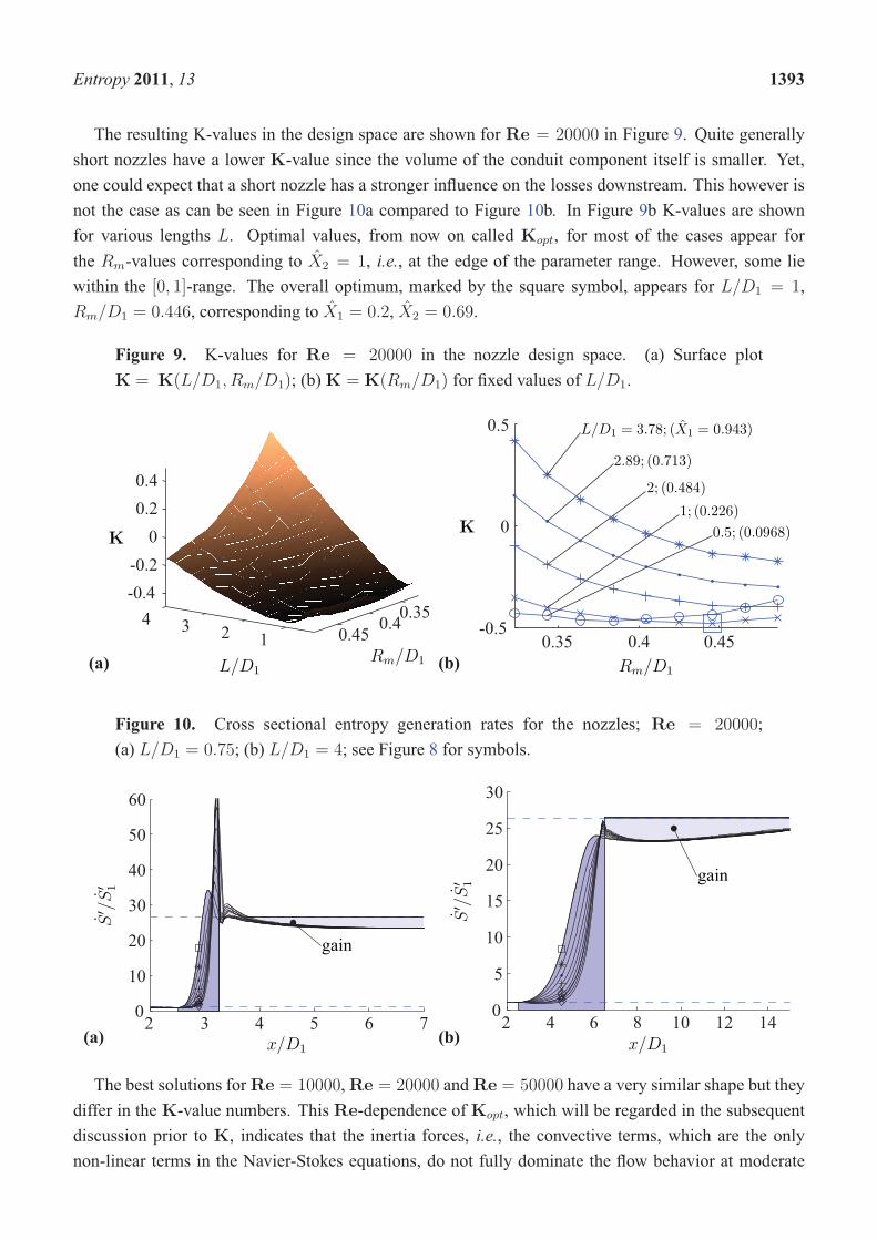
The resulting K-values in the design space are shown for Re = 20000 in Figure 9. Quite generallyshort nozzles have a lower K-value since the volume of the conduit component itself is smaller. Yet,one could expect that a short nozzle has a stronger influence on the losses downstream. This however isnot the case as can be seen in Figure 10a compared to Figure 10b. In Figure 9b K-values are shownfor various lengths L. Optimal values, from now on called Kopt, for most of the cases appear forthe Rm-values corresponding to X2 = 1, i.e., at the edge of the parameter range. However, some liewithin the [0, 1]-range. The overall optimum, marked by the square symbol, appears for L/D1 = 1,Rm/D1 = 0.446, corresponding to X1 = 0.2, X2 = 0.69.
Figure 9. K-values for Re = 20000 in the nozzle design space. (a) Surface plotK = K(L/D1, Rm/D1); (b)K = K(Rm/D1) for fixed values of L/D1.
(a) L/D1
Rm/D1
K
1234 0.350.40.45
-0.4-0.200.20.4
(b)
0.5; (0.0968)
1; (0.226)
2; (0.484)
2.89; (0.713)
L/D1 = 3.78; (X1 = 0.943)
Rm/D1
K
0.35 0.4 0.45-0.5
0
0.5
Figure 10. Cross sectional entropy generation rates for the nozzles; Re = 20000;(a) L/D1 = 0.75; (b) L/D1 = 4; see Figure 8 for symbols.
(a)
gain
x/D1
S′ /S′ 1
2 3 4 5 6 70
10
20
30
40
50
60
(b)
gain
x/D1
S′ /S′ 1
2 4 6 8 10 12 140
5
10
15
20
25
30
The best solutions forRe = 10000,Re = 20000 andRe = 50000 have a very similar shape but theydiffer in the K-value numbers. This Re-dependence of Kopt, which will be regarded in the subsequentdiscussion prior to K, indicates that the inertia forces, i.e., the convective terms, which are the onlynon-linear terms in the Navier-Stokes equations, do not fully dominate the flow behavior at moderate
Entropy 2011, 13 1394
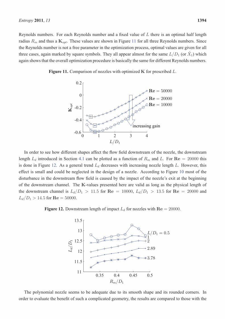
Reynolds numbers. For each Reynolds number and a fixed value of L there is an optimal half lengthradius Rm and thus a Kopt. These values are shown in Figure 11 for all three Reynolds numbers. Sincethe Reynolds number is not a free parameter in the optimization process, optimal values are given for allthree cases, again marked by square symbols. They all appear almost for the same L/D1 (or X1) whichagain shows that the overall optimization procedure is basically the same for different Reynolds numbers.
Figure 11. Comparison of nozzles with optimizedK for prescribed L.K
opt
L/D1
Re = 10000
Re = 20000
Re = 50000
increasing gain
0 1 2 3 4-0.6
-0.4
-0.2
0
0.2
In order to see how different shapes affect the flow field downstream of the nozzle, the downstreamlength Ld introduced in Section 4.1 can be plotted as a function of Rm and L. For Re = 20000 thisis done in Figure 12. As a general trend Ld decreases with increasing nozzle length L. However, thiseffect is small and could be neglected in the design of a nozzle. According to Figure 10 most of thedisturbance in the downstream flow field is caused by the impact of the nozzle’s exit at the beginningof the downstream channel. The K-values presented here are valid as long as the physical length ofthe downstream channel is Ld/D1 > 11.5 for Re = 10000, Ld/D1 > 13.5 for Re = 20000 andLd/D1 > 14.5 forRe = 50000.
Figure 12. Downstream length of impact Ld for nozzles withRe = 20000.
L/D1 = 0.512
2.89
3.78
Rm/D1
Ld/D
1
0.35 0.4 0.45 0.511
11.5
12
12.5
13
13.5
The polynomial nozzle seems to be adequate due to its smooth shape and its rounded corners. Inorder to evaluate the benefit of such a complicated geometry, the results are compared to those with the
Entropy 2011, 13 1395
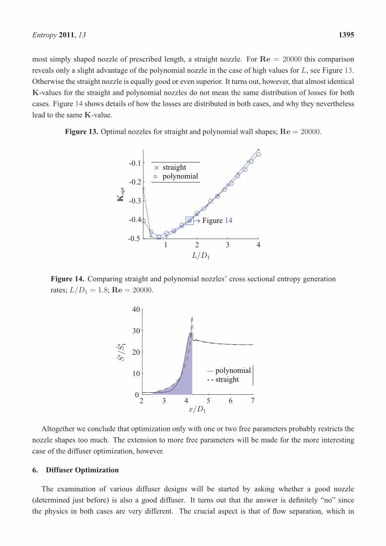
most simply shaped nozzle of prescribed length, a straight nozzle. For Re = 20000 this comparisonreveals only a slight advantage of the polynomial nozzle in the case of high values for L, see Figure 13.Otherwise the straight nozzle is equally good or even superior. It turns out, however, that almost identicalK-values for the straight and polynomial nozzles do not mean the same distribution of losses for bothcases. Figure 14 shows details of how the losses are distributed in both cases, and why they neverthelesslead to the sameK-value.
Figure 13. Optimal nozzles for straight and polynomial wall shapes;Re = 20000.K
Altogether we conclude that optimization only with one or two free parameters probably restricts thenozzle shapes too much. The extension to more free parameters will be made for the more interestingcase of the diffuser optimization, however.
6. Diffuser Optimization
The examination of various diffuser designs will be started by asking whether a good nozzle(determined just before) is also a good diffuser. It turns out that the answer is definitely “no” sincethe physics in both cases are very different. The crucial aspect is that of flow separation, which in
Entropy 2011, 13 1396
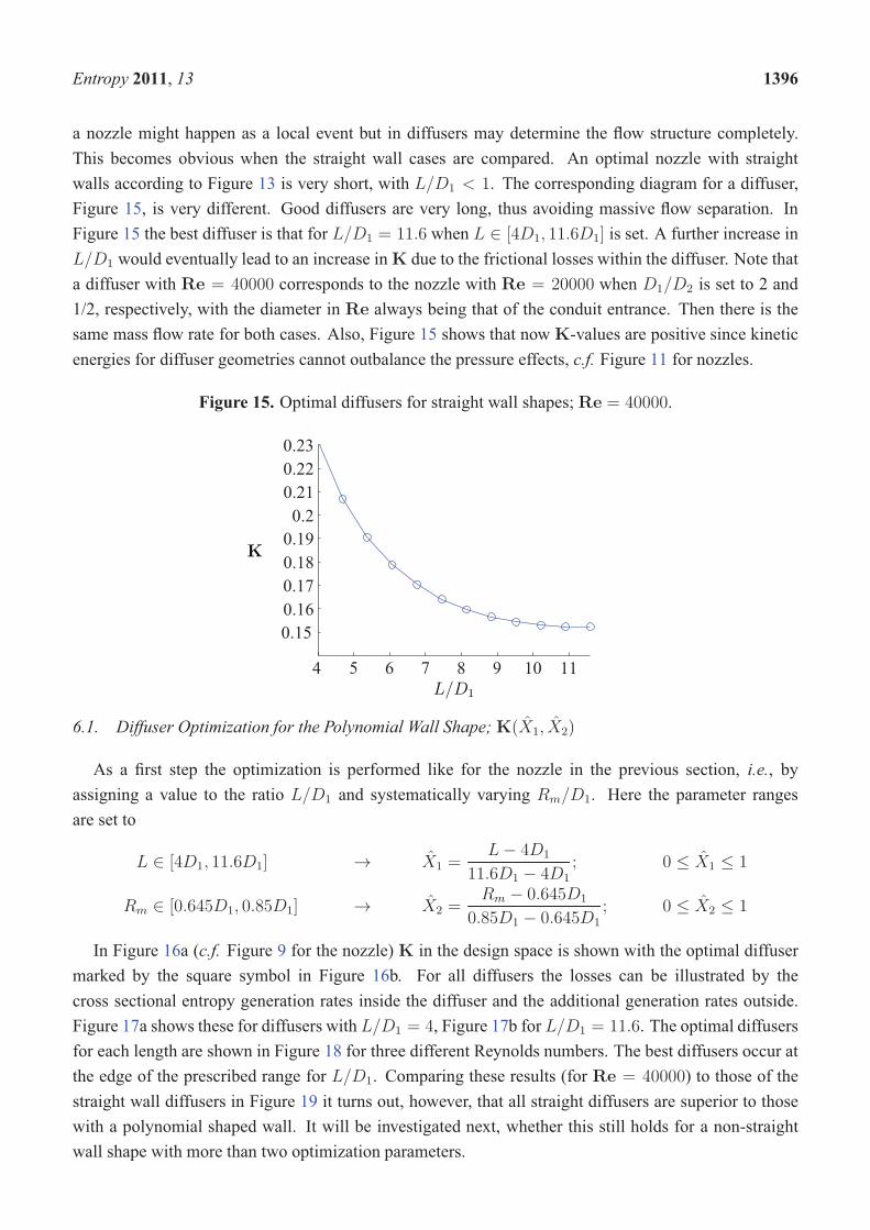
a nozzle might happen as a local event but in diffusers may determine the flow structure completely.This becomes obvious when the straight wall cases are compared. An optimal nozzle with straightwalls according to Figure 13 is very short, with L/D1 < 1. The corresponding diagram for a diffuser,Figure 15, is very different. Good diffusers are very long, thus avoiding massive flow separation. InFigure 15 the best diffuser is that for L/D1 = 11.6 when L ∈ [4D1, 11.6D1] is set. A further increase inL/D1 would eventually lead to an increase inK due to the frictional losses within the diffuser. Note thata diffuser with Re = 40000 corresponds to the nozzle with Re = 20000 when D1/D2 is set to 2 and1/2, respectively, with the diameter in Re always being that of the conduit entrance. Then there is thesame mass flow rate for both cases. Also, Figure 15 shows that nowK-values are positive since kineticenergies for diffuser geometries cannot outbalance the pressure effects, c.f. Figure 11 for nozzles.
Figure 15. Optimal diffusers for straight wall shapes;Re = 40000.
K
L/D1
4 5 6 7 8 9 10 11
0.150.160.170.180.190.20.210.220.23
6.1. Diffuser Optimization for the Polynomial Wall Shape;K(X1, X2)
As a first step the optimization is performed like for the nozzle in the previous section, i.e., byassigning a value to the ratio L/D1 and systematically varying Rm/D1. Here the parameter rangesare set to
L ∈ [4D1, 11.6D1] → X1 =L− 4D1
11.6D1 − 4D1
; 0 ≤ X1 ≤ 1
Rm ∈ [0.645D1, 0.85D1] → X2 =Rm − 0.645D1
0.85D1 − 0.645D1
; 0 ≤ X2 ≤ 1
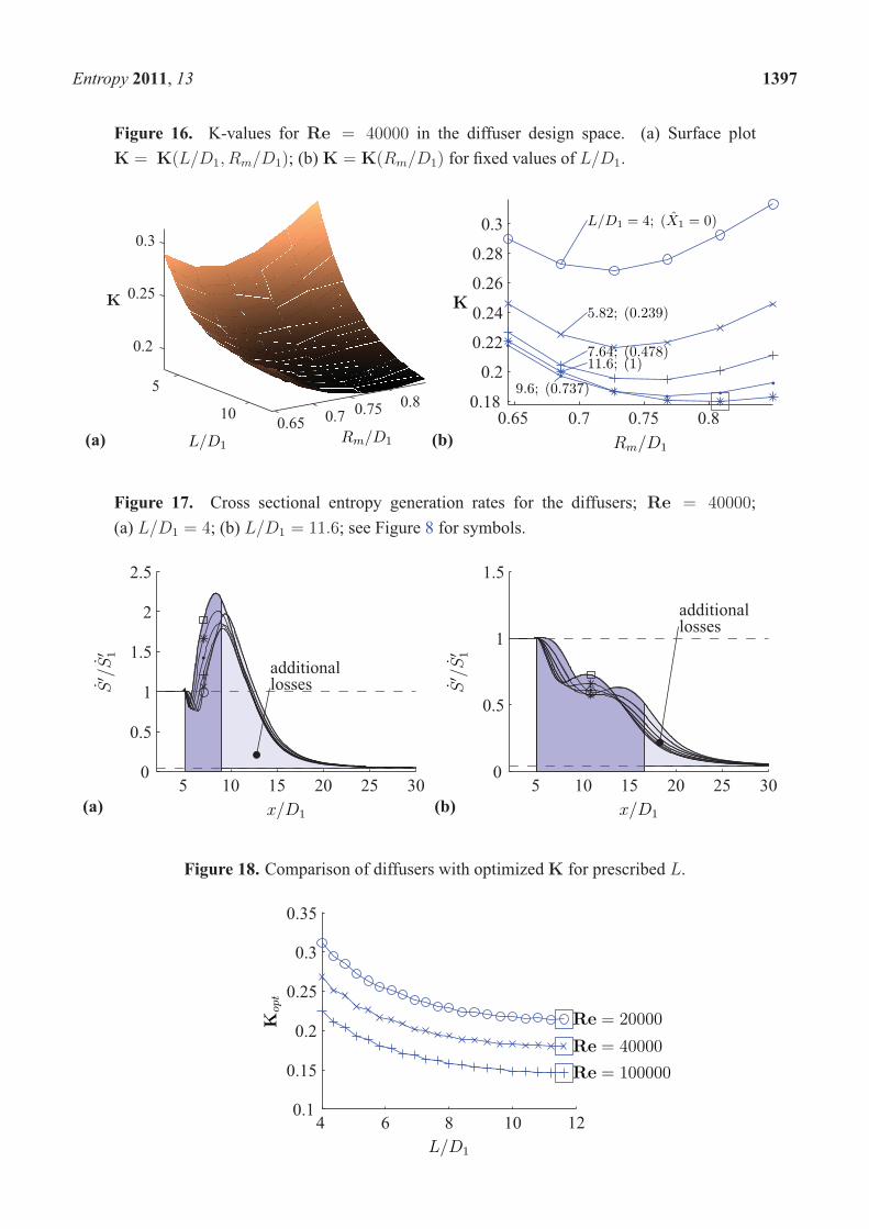
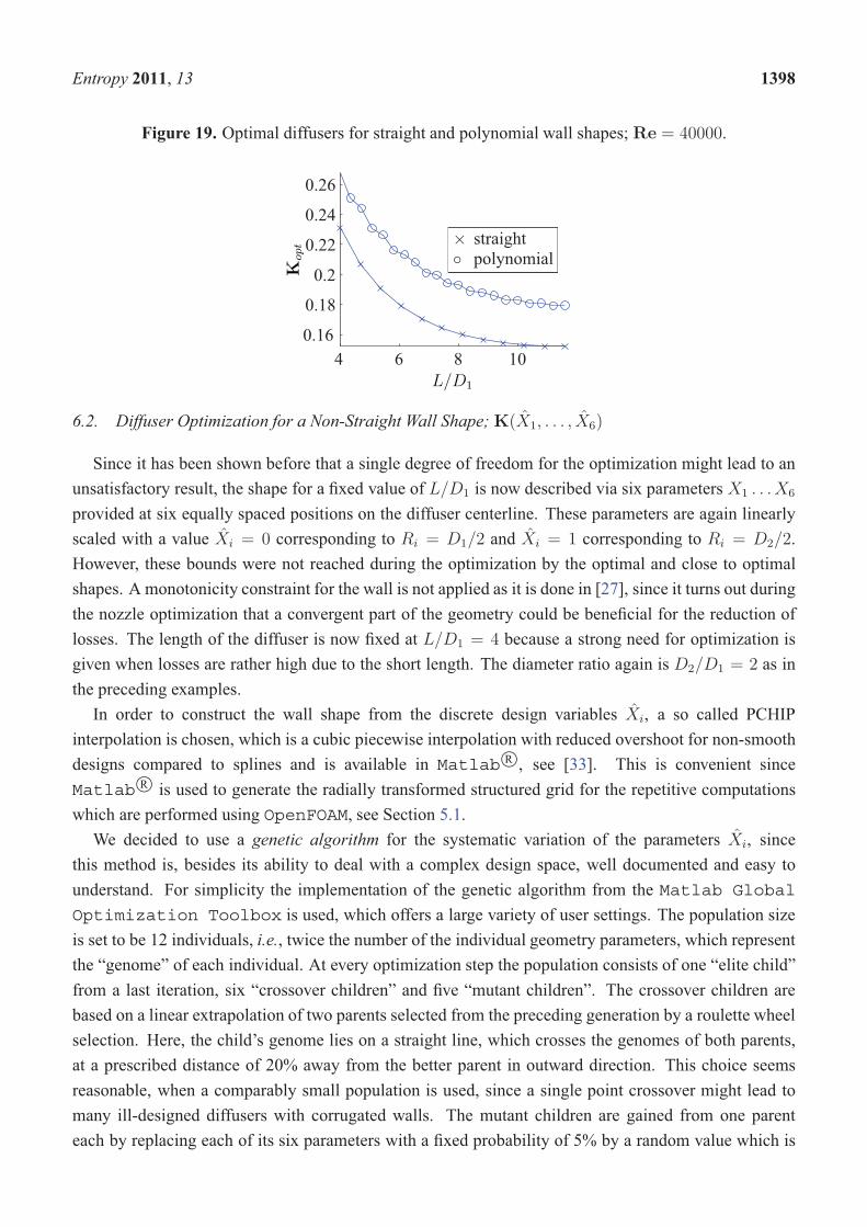
In Figure 16a (c.f. Figure 9 for the nozzle) K in the design space is shown with the optimal diffusermarked by the square symbol in Figure 16b. For all diffusers the losses can be illustrated by thecross sectional entropy generation rates inside the diffuser and the additional generation rates outside.Figure 17a shows these for diffusers with L/D1 = 4, Figure 17b for L/D1 = 11.6. The optimal diffusersfor each length are shown in Figure 18 for three different Reynolds numbers. The best diffusers occur atthe edge of the prescribed range for L/D1. Comparing these results (for Re = 40000) to those of thestraight wall diffusers in Figure 19 it turns out, however, that all straight diffusers are superior to thosewith a polynomial shaped wall. It will be investigated next, whether this still holds for a non-straightwall shape with more than two optimization parameters.
Entropy 2011, 13 1397
Figure 16. K-values for Re = 40000 in the diffuser design space. (a) Surface plotK = K(L/D1, Rm/D1); (b)K = K(Rm/D1) for fixed values of L/D1.
(a) L/D1Rm/D1
K
5
10 0.65 0.7 0.750.8
0.2
0.25
0.3
(b)
L/D1 = 4; (X1 = 0)
5.82; (0.239)
7.64; (0.478)
9.6; (0.737)
11.6; (1)
Rm/D1
K
0.65 0.7 0.75 0.80.18
0.2
0.22
0.24
0.26
0.28
0.3
Figure 17. Cross sectional entropy generation rates for the diffusers; Re = 40000;(a) L/D1 = 4; (b) L/D1 = 11.6; see Figure 8 for symbols.
(a)
additionallosses
x/D1
S′ /S′ 1
5 10 15 20 25 300
0.5
1
1.5
2
2.5
(b)
additionallosses
x/D1
S′ /S′ 1
5 10 15 20 25 300
0.5
1
1.5
Figure 18. Comparison of diffusers with optimizedK for prescribed L.
Kopt
L/D1
Re = 20000
Re = 40000
Re = 100000
4 6 8 10 120.1
0.15
0.2
0.25
0.3
0.35
Entropy 2011, 13 1398
Figure 19. Optimal diffusers for straight and polynomial wall shapes; Re = 40000.
Kopt
L/D1
× straight◦ polynomial
4 6 8 100.16
0.18
0.2
0.22
0.24
0.26
6.2. Diffuser Optimization for a Non-Straight Wall Shape;K(X1, . . . , X6)
Since it has been shown before that a single degree of freedom for the optimization might lead to anunsatisfactory result, the shape for a fixed value of L/D1 is now described via six parameters X1 . . .X6
provided at six equally spaced positions on the diffuser centerline. These parameters are again linearlyscaled with a value Xi = 0 corresponding to Ri = D1/2 and Xi = 1 corresponding to Ri = D2/2.However, these bounds were not reached during the optimization by the optimal and close to optimalshapes. A monotonicity constraint for the wall is not applied as it is done in [27], since it turns out duringthe nozzle optimization that a convergent part of the geometry could be beneficial for the reduction oflosses. The length of the diffuser is now fixed at L/D1 = 4 because a strong need for optimization isgiven when losses are rather high due to the short length. The diameter ratio again is D2/D1 = 2 as inthe preceding examples.In order to construct the wall shape from the discrete design variables Xi, a so called PCHIP
this method is, besides its ability to deal with a complex design space, well documented and easy tounderstand. For simplicity the implementation of the genetic algorithm from the Matlab Global
Optimization Toolbox is used, which offers a large variety of user settings. The population sizeis set to be 12 individuals, i.e., twice the number of the individual geometry parameters, which representthe “genome” of each individual. At every optimization step the population consists of one “elite child”from a last iteration, six “crossover children” and five “mutant children”. The crossover children arebased on a linear extrapolation of two parents selected from the preceding generation by a roulette wheelselection. Here, the child’s genome lies on a straight line, which crosses the genomes of both parents,at a prescribed distance of 20% away from the better parent in outward direction. This choice seemsreasonable, when a comparably small population is used, since a single point crossover might lead tomany ill-designed diffusers with corrugated walls. The mutant children are gained from one parenteach by replacing each of its six parameters with a fixed probability of 5% by a random value which is
Entropy 2011, 13 1399
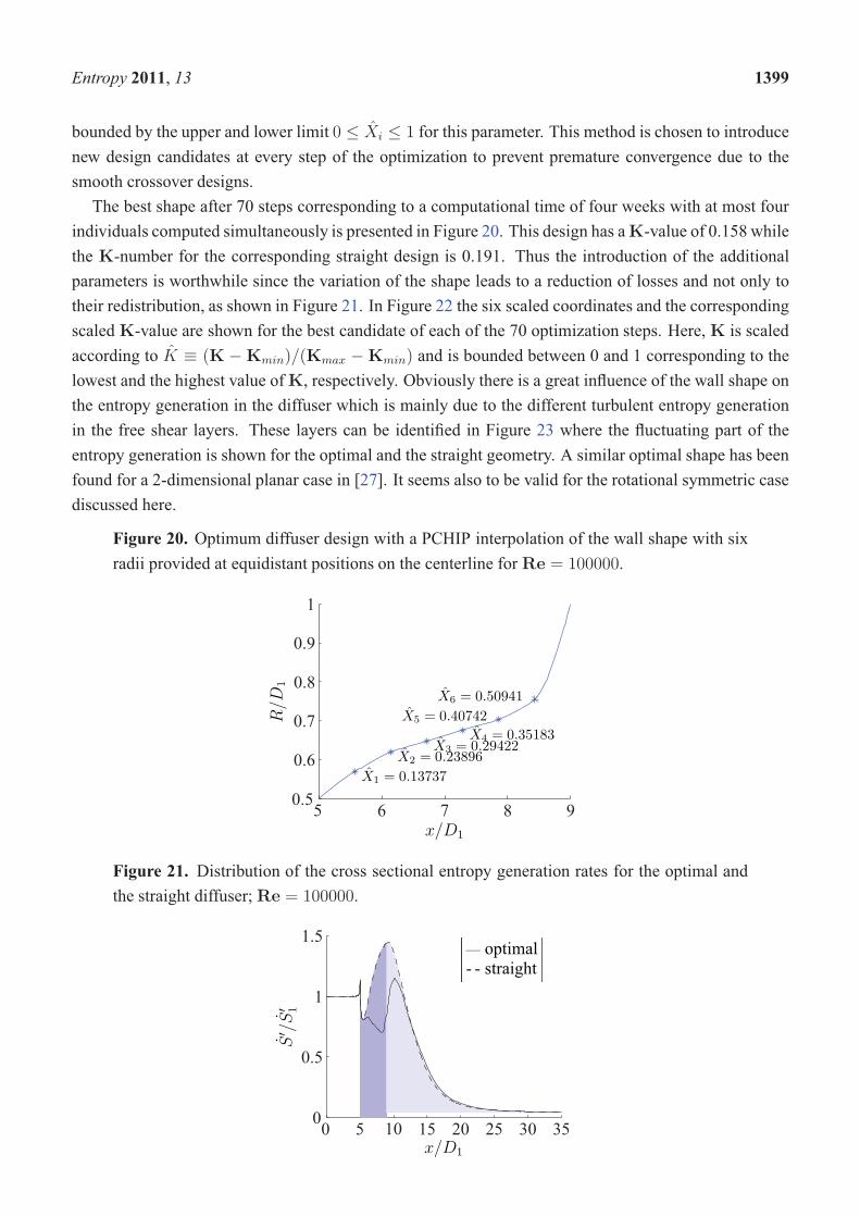
bounded by the upper and lower limit 0 ≤ Xi ≤ 1 for this parameter. This method is chosen to introducenew design candidates at every step of the optimization to prevent premature convergence due to thesmooth crossover designs.The best shape after 70 steps corresponding to a computational time of four weeks with at most four
individuals computed simultaneously is presented in Figure 20. This design has aK-value of 0.158 whilethe K-number for the corresponding straight design is 0.191. Thus the introduction of the additionalparameters is worthwhile since the variation of the shape leads to a reduction of losses and not only totheir redistribution, as shown in Figure 21. In Figure 22 the six scaled coordinates and the correspondingscaled K-value are shown for the best candidate of each of the 70 optimization steps. Here, K is scaledaccording to K ≡ (K −Kmin)/(Kmax −Kmin) and is bounded between 0 and 1 corresponding to thelowest and the highest value ofK, respectively. Obviously there is a great influence of the wall shape onthe entropy generation in the diffuser which is mainly due to the different turbulent entropy generationin the free shear layers. These layers can be identified in Figure 23 where the fluctuating part of theentropy generation is shown for the optimal and the straight geometry. A similar optimal shape has beenfound for a 2-dimensional planar case in [27]. It seems also to be valid for the rotational symmetric casediscussed here.
Figure 20. Optimum diffuser design with a PCHIP interpolation of the wall shape with sixradii provided at equidistant positions on the centerline forRe = 100000.
X1 = 0.13737
X2 = 0.23896X3 = 0.29422
X4 = 0.35183
X5 = 0.40742
X6 = 0.50941
x/D1
R/D
1
5 6 7 8 90.5
0.6
0.7
0.8
0.9
1
Figure 21. Distribution of the cross sectional entropy generation rates for the optimal andthe straight diffuser;Re = 100000.
x/D1
S′ /S′ 1
— optimal- - straight
0 5 10 15 20 25 30 350
0.5
1
1.5
Entropy 2011, 13 1400
Figure 22. Visualization of the investigated design space in parallel coordinates (only eliteindividuals from every generation are shown);Re = 100000.
CoordinateValue
X1 X2 X3 X4 X5 X6 K0
0.2
0.4
0.6
0.8
1
Figure 23. Fluctuating part (S ′′′)′ of the entropy generation rates S ′′′; light: high values,nonlinear scale.
optimal
straight
7. Conclusions
In this paper it has been shown how the entropy generation field obtained from a numerical simulationcan be used to compute the K-value of conduit components as the target for optimization. Besidesits advantages in the single objective optimization process, the ability of the second law analysis tocontribute to the interpretation of the optimization results was illustrated for different nozzle and diffusergeometries. It was demonstrated how plots of the entropy generation in streamwise direction as well asupstream and downstream lengths of influence can be used to quantify the distribution of losses. Thus,for different strategies of shape optimization it could be checked whether a reduction of losses at a certainpart of a conduit component led to an improvement of the whole component or only to the redistributionof losses within the component and its downstream section.
Acknowledgements
The authors gratefully acknowledge the support of the DFG (Deutsche Forschungsgemeinschaft).
Entropy 2011, 13 1401
References
1. Herwig, H. The role of entropy generation in momentum and heat transfer. In Proceedingsof the International Heat Transfer Conference, Washington D.C., USA, 8–13 August 2010; No.IHTC14-23348.
2. Schmandt, B.; Herwig, H. Internal flow losses: A fresh look at old concepts. J. Fluids Eng. 2011,133, 051201.
3. Moran, M.; Shapiro, H. Fundamentals of Engineering Thermodynamics, 3rd ed.; John Wiley &Sons, Inc.: New York, NY, USA, 1996.
4. Baehr, H. Thermodynamik, 14th ed.; Springer-Verlag: Berlin, Germany, 2009.5. Herwig, H.; Kautz, C. Technische Thermodynamik; Pearson Studium: Munchen, Germany, 2007.6. Dugdale, J. Entropy and Its Physical Meaning.; Cambridge University Press: Cambridge, UK,1996.
7. Atkins, P. The Second Law; Scientific American Books, W.H. Freeman and Company: New York,NY, USA, 1984.
8. Goldstein, M.; Goldstein, I. The Refrigerator and the Universe; Harvard University Press:Cambridge, MA, USA, 1993.
9. Falk, G.; Ruppel, W. Energie und Entropie; Springer-Verlag: Berlin, Germany, 1976.10. Lieb, E.; Yngvason, J. A fresh look at entropy and the second law of thermodynamics. Physics
Today 2000, 11, 106.11. Beretta, G.; Ghoniem, A.; Hatsopoulos, G. Meeting the entropy challenge. AIP Conference
Proceedings 2008, CP 1033, 382.12. Bejan, A. The concept of irreversibility in heat exchanger design: counter-flow heat exchangers
for gas-to-gas applications. J. Heat Tran. 1977, 99, 274–380.13. Sekulic, D. Entropy generation in a heat exchanger. Heat Tran. Eng. 1986, 7, 83–88.14. Gaggioli, R. Second law analysis for process and energy engineering. In Efficiency and Costing,
Second Laws Analysis of Processes; American Chemical Society: New York, NY, USA, 1983.15. Bejan, A. A study of entropy generation in fundamental convective heat transfer. J. Heat Tran.
1979, 101, 718–725.16. Bejan, A. Entropy Generation through Heat and Fluid Flow; John Wiley & Sons: New York, NY,
USA, 1982.17. Bejan, A. Entropy Generation Minimization; CRC Press: Boca Raton, New York, NY, 1996.18. Hesselgreaves, J. Rationalisation of second law analysis of heat exchangers. J. Heat Mass Tran.
2000, 43, 4189–4204.19. Herwig, H.; Kock, F. Direct and indirect methods of calculating entropy generation rates in
turbulent convective heat transfer problems. Heat Mass Tran. 2007, 43, 207–215.20. Anand, D. Second law analysis of solar powered absorption cooling cycles and systems. J. Sol.
Energy Eng. 1984, 106, 291–298.21. Nuwayhid, R.; Moukalled, F.; Noueihed, N. On entropy generation in thermoelectric devices.
Energ. Conv. Manage. 2000, 41, 891–914.
Entropy 2011, 13 1402
22. Assad, E. Thermodynamic analysis of an irreversible MHD power plant. Int. J. Energ. Res. 2000,24, 865–875.
23. Shiba, T.; Bejan, A. Thermodynamic optimization of geometric structure in the counterflow heatexchanger for an environmental control system. Energy 2001, 26, 493–511.
24. Saidi, M.; Yazdi, M. Exergy model of a vortex tube system with experimental results. Energy1999, 24, 625–632.
25. San, J.; Jan, C. Second law analysis of a wet crossflow heat exchanger. Energy 2000, 25, 939–955.26. Ko, T.; Ting, K. Entropy generation and optimal analysis for laminar forced convection in curved
rectangular ducts: A numerical study. Int. J. Therm. Sci. 2006, 45, 138–150.27. Madsen, J.I.; Shyy, W. Response surface techniques for diffuser shape optimization. AIAA J. 2000,
38, 1512–1518.28. Ghosh, S.; Pratihat, D.; Das, P. An evolutionary optimization of diffuser shapes based on CFD
simulations. Int. J. Numer. Meth. Fluids 2010, 63, 1147–1166.29. Thevenin, D.; Janiga, D. Optimization and Computational Fluid Dynamics; Springer-Verlag:
Berlin, Heidelberg, Germany, 2008.30. Kock, F.; Herwig, H. Local entropy production in turbulent shear flows: A high Reynolds number
model with wall functions. Int. J. Heat Mass Tran. 2004, 47, 2205–2215.31. Menter, F. Improved two-equation k-omega turbulence models for aerodynamic flows. NASA Tech.
Memorand. 1992, 103975.32. OpenFOAM User Guide, Version 1.6; OpenCFD, Ltd.: Reading, Berkshire, UK, 2009.33. Matlab 7: Mathematics, from Mathworks Userguide 2010a; The MathWorks, Inc.: Natick, MA,