Diffusion Jan K.G. Dhont This document has been published in Manuel Angst, Thomas Brückel, Dieter Richter, Reiner Zorn (Eds.): Scattering Methods for Condensed Matter Research: Towards Novel Applications at Future Sources Lecture Notes of the 43rd IFF Spring School 2012 Schriften des Forschungszentrums Jülich / Reihe Schlüsseltechnologien / Key Tech- nologies, Vol. 33 JCNS, PGI, ICS, IAS Forschungszentrum Jülich GmbH, JCNS, PGI, ICS, IAS, 2012 ISBN: 978-3-89336-759-7 All rights reserved.
Transcript
Diffusion
Jan K.G. Dhont
This document has been published in
Manuel Angst, Thomas Brückel, Dieter Richter, Reiner Zorn (Eds.):Scattering Methods for Condensed Matter Research: Towards Novel Applications atFuture SourcesLecture Notes of the 43rd IFF Spring School 2012Schriften des Forschungszentrums Jülich / Reihe Schlüsseltechnologien / Key Tech-nologies, Vol. 33JCNS, PGI, ICS, IASForschungszentrum Jülich GmbH, JCNS, PGI, ICS, IAS, 2012ISBN: 978-3-89336-759-7All rights reserved.
1Lecture Notes of the 43rd IFF Spring School “Scattering Methods for Condensed Matter Research: TowardsNovel Applications at Future Sources” (Forschungszentrum Julich, 2012). All rights reserved.
B3.2 Jan K.G. Dhont
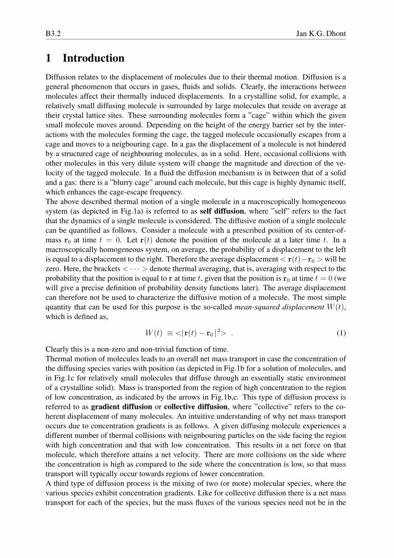
1 IntroductionDiffusion relates to the displacement of molecules due to their thermal motion. Diffusion is ageneral phenomenon that occurs in gases, fluids and solids. Clearly, the interactions betweenmolecules affect their thermally induced displacements. In a crystalline solid, for example, arelatively small diffusing molecule is surrounded by large molecules that reside on average attheir crystal lattice sites. These surrounding molecules form a ”cage” within which the givensmall molecule moves around. Depending on the height of the energy barrier set by the inter-actions with the molecules forming the cage, the tagged molecule occasionally escapes from acage and moves to a neigbouring cage. In a gas the displacement of a molecule is not hinderedby a structured cage of neighbouring molecules, as in a solid. Here, occasional collisions withother molecules in this very dilute system will change the magnitude and direction of the ve-locity of the tagged molecule. In a fluid the diffusion mechanism is in between that of a solidand a gas: there is a ”blurry cage” around each molecule, but this cage is highly dynamic itself,which enhances the cage-escape frequency.The above described thermal motion of a single molecule in a macroscopically homogeneoussystem (as depicted in Fig.1a) is referred to as self diffusion, where ”self” refers to the factthat the dynamics of a single molecule is considered. The diffusive motion of a single moleculecan be quantified as follows. Consider a molecule with a prescribed position of its center-of-mass r0 at time t = 0. Let r(t) denote the position of the molecule at a later time t. In amacroscopically homogeneous system, on average, the probability of a displacement to the leftis equal to a displacement to the right. Therefore the average displacement < r(t)−r0 > will bezero. Here, the brackets < · · · > denote thermal averaging, that is, averaging with respect to theprobability that the position is equal to r at time t, given that the position is r0 at time t = 0 (wewill give a precise definition of probability density functions later). The average displacementcan therefore not be used to characterize the diffusive motion of a molecule. The most simplequantity that can be used for this purpose is the so-called mean-squared displacement W (t),which is defined as,
W (t) ≡ <|r(t)− r0 | 2> . (1)
Clearly this is a non-zero and non-trivial function of time.Thermal motion of molecules leads to an overall net mass transport in case the concentration ofthe diffusing species varies with position (as depicted in Fig.1b for a solution of molecules, andin Fig.1c for relatively small molecules that diffuse through an essentially static environmentof a crystalline solid). Mass is transported from the region of high concentration to the regionof low concentration, as indicated by the arrows in Fig.1b,c. This type of diffusion process isreferred to as gradient diffusion or collective diffusion, where ”collective” refers to the co-herent displacement of many molecules. An intuitive understanding of why net mass transportoccurs due to concentration gradients is as follows. A given diffusing molecule experiences adifferent number of thermal collisions with neignbouring particles on the side facing the regionwith high concentration and that with low concentration. This results in a net force on thatmolecule, which therefore attains a net velocity. There are more collisions on the side wherethe concentration is high as compared to the side where the concentration is low, so that masstransport will typically occur towards regions of lower concentration.A third type of diffusion process is the mixing of two (or more) molecular species, where thevarious species exhibit concentration gradients. Like for collective diffusion there is a net masstransport for each of the species, but the mass fluxes of the various species need not be in the
Diffusion B3.3
(a) (b) (c) (d)
self diffusion collective diffusion collective diffusion inter diffusion
(a) (b) (c) (d)
self diffusion collective diffusion collective diffusion inter diffusion
Fig. 1: The three types of diffusion processes. (a) ”self diffusion”: the thermal motion of asingle molecule, here for molecule within a crystalline solid with open interstitial positions.(b) ”collective diffusion”: a concentration gradient in a solution of molecules induced diffu-sive mass transport from the region of high concentration to the region of low concentration(as indicated by the arrow. (c) again collective diffusion, but now of small molecules (in red)through an essentially static environment of a crystalline solid. (d) ”Inter diffusion”: two dif-ferent molecules (in blue and red), with opposite concentration gradients, mix due to diffusion.The arrows indicate the direction of net mass transport of the two components.
same direction. This diffusion process is referred to as inter diffusion, and is depicted in Fig.1d,where the directions of the mass fluxes are indicated by the arrows.
Within the general classification of diffusion processes in self-, collective, and inter-diffusion,there is a great variety of different types of diffusion mechanisms for various types of systems.Some of these will be discussed quantitatively, and some only on a qualitative level. In thischapter we will focus on self- and collective-diffusion. Inter-diffusion will not be discussed.
Diffusive mass transport in stable systems is from regions of high concentration to low concen-tration. For thermodynamically unstable systems, however, strong attractive forces betweenmolecules favor increase of concentration, where molecules are on average in each other’svicinity. The energy is lowered by increasing the concentration in part of the system due tothe strong attractive interactions. Diffusion is now ”uphill”, from regions of low concentrationto high concentration. Inhomogeneities thus increase in time, which is a kinetic stage duringphase separation. The end-state is a coexistence between two phases. The initial stage of phaseseparation from an initially homogeneous, unstable system is discussed in section 4.
2 Self Diffusion
In this section we shall first develop a simple model in one dimension, where a molecule resideson discrete positions and can jump between these positions with a certain prescribed probability.In subsection 2.2 the discrete model will be cast in a continuum description, which allows forthe explicit analysis of the time evolution of the probability density function for the positioncoordinate of a diffusing molecule. In subsection 2.3, the diffusion of a molecule in a periodicenergy landscape will be analyzed, and compared to experiments. Finally, in subsection 2.4 afew other types of self-diffusion processes will be addressed on a qualitative level.
B3.4 Jan K.G. Dhont
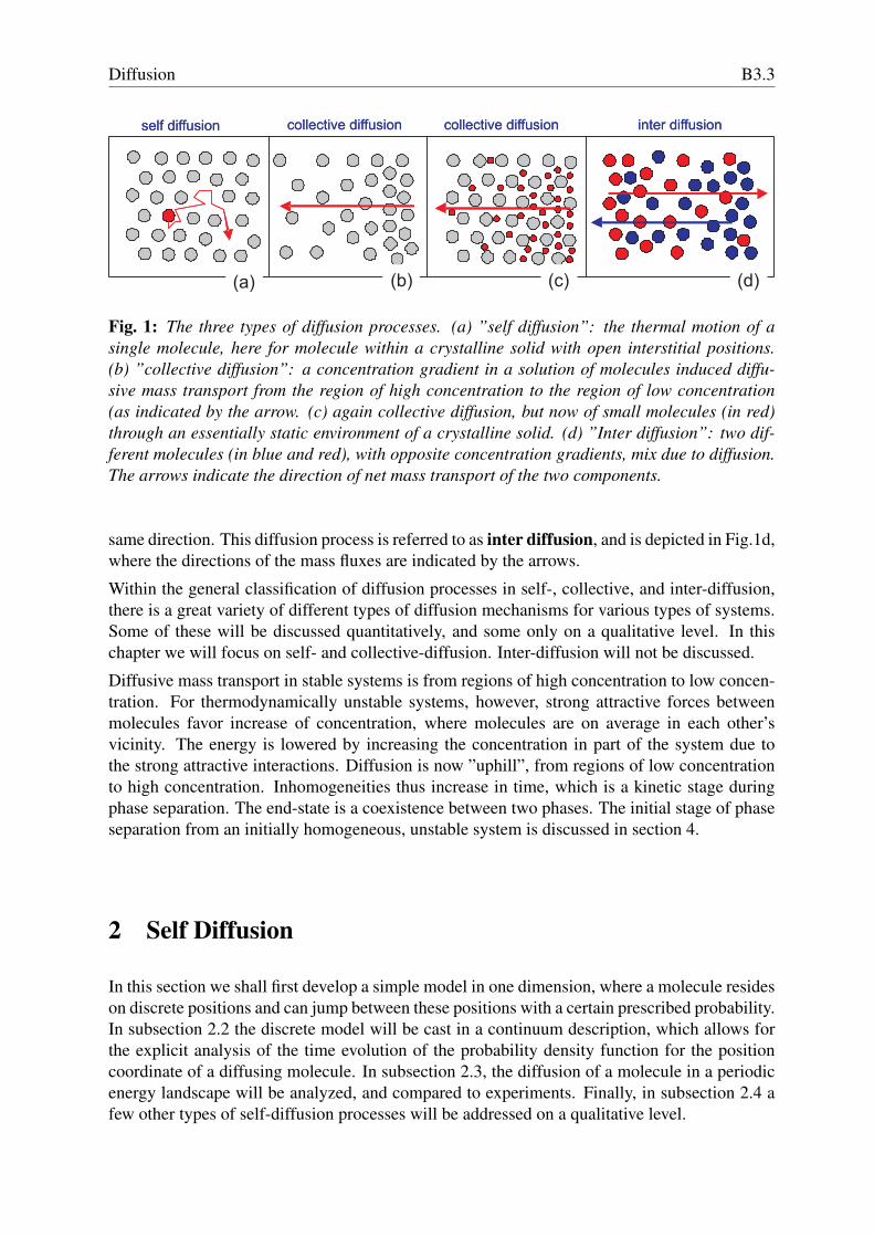
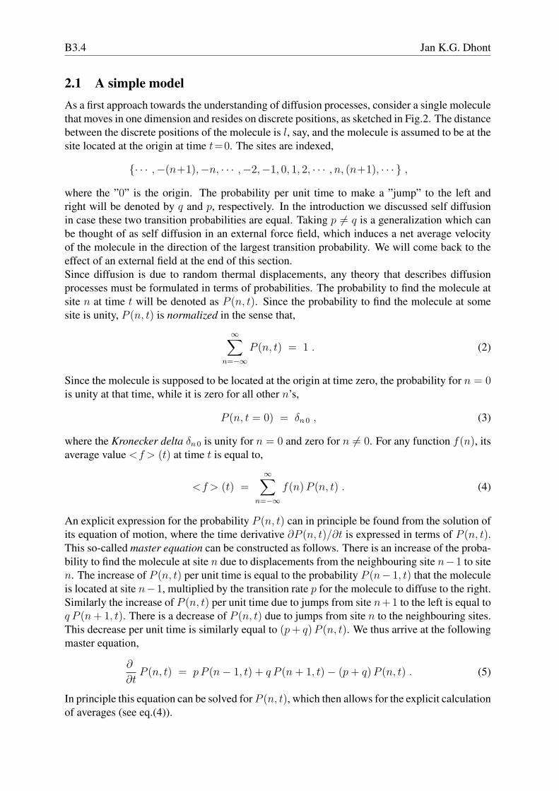
2.1 A simple modelAs a first approach towards the understanding of diffusion processes, consider a single moleculethat moves in one dimension and resides on discrete positions, as sketched in Fig.2. The distancebetween the discrete positions of the molecule is l, say, and the molecule is assumed to be at thesite located at the origin at time t=0. The sites are indexed,
where the ”0” is the origin. The probability per unit time to make a ”jump” to the left andright will be denoted by q and p, respectively. In the introduction we discussed self diffusionin case these two transition probabilities are equal. Taking p 6= q is a generalization which canbe thought of as self diffusion in an external force field, which induces a net average velocityof the molecule in the direction of the largest transition probability. We will come back to theeffect of an external field at the end of this section.Since diffusion is due to random thermal displacements, any theory that describes diffusionprocesses must be formulated in terms of probabilities. The probability to find the molecule atsite n at time t will be denoted as P (n, t). Since the probability to find the molecule at somesite is unity, P (n, t) is normalized in the sense that,
∞∑n=−∞
P (n, t) = 1 . (2)
Since the molecule is supposed to be located at the origin at time zero, the probability for n = 0is unity at that time, while it is zero for all other n’s,
P (n, t = 0) = δn 0 , (3)
where the Kronecker delta δn 0 is unity for n = 0 and zero for n 6= 0. For any function f(n), itsaverage value <f > (t) at time t is equal to,
<f > (t) =∞∑
n=−∞f(n) P (n, t) . (4)
An explicit expression for the probability P (n, t) can in principle be found from the solution ofits equation of motion, where the time derivative ∂P (n, t)/∂t is expressed in terms of P (n, t).This so-called master equation can be constructed as follows. There is an increase of the proba-bility to find the molecule at site n due to displacements from the neighbouring site n−1 to siten. The increase of P (n, t) per unit time is equal to the probability P (n− 1, t) that the moleculeis located at site n−1, multiplied by the transition rate p for the molecule to diffuse to the right.Similarly the increase of P (n, t) per unit time due to jumps from site n+1 to the left is equal toq P (n + 1, t). There is a decrease of P (n, t) due to jumps from site n to the neighbouring sites.This decrease per unit time is similarly equal to (p + q) P (n, t). We thus arrive at the followingmaster equation,
In principle this equation can be solved for P (n, t), which then allows for the explicit calculationof averages (see eq.(4)).
Diffusion B3.5
pq
0 1 2 3 4 …..…….. -1-2-3-4
pq
0 1 2 3 4 …..…….. -1-2-3-4
l
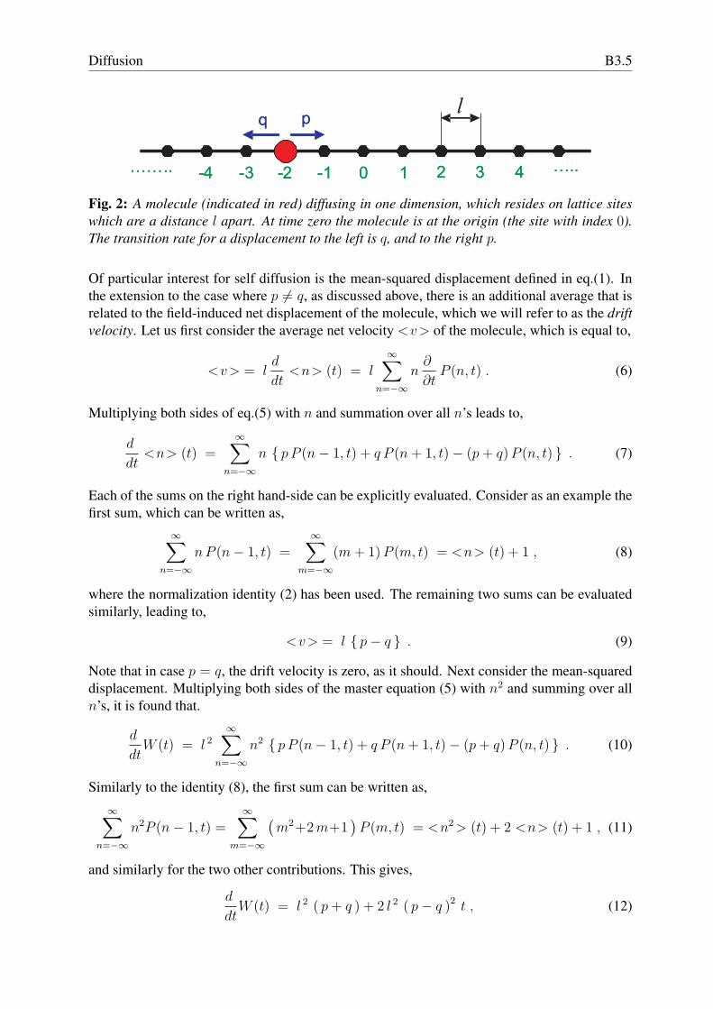
Fig. 2: A molecule (indicated in red) diffusing in one dimension, which resides on lattice siteswhich are a distance l apart. At time zero the molecule is at the origin (the site with index 0).The transition rate for a displacement to the left is q, and to the right p.
Of particular interest for self diffusion is the mean-squared displacement defined in eq.(1). Inthe extension to the case where p 6= q, as discussed above, there is an additional average that isrelated to the field-induced net displacement of the molecule, which we will refer to as the driftvelocity. Let us first consider the average net velocity <v> of the molecule, which is equal to,
<v> = ld
dt<n> (t) = l
∞∑n=−∞
n∂
∂tP (n, t) . (6)
Multiplying both sides of eq.(5) with n and summation over all n’s leads to,
d
dt<n> (t) =
∞∑n=−∞
n { pP (n− 1, t) + q P (n + 1, t)− (p + q) P (n, t) } . (7)
Each of the sums on the right hand-side can be explicitly evaluated. Consider as an example thefirst sum, which can be written as,
∞∑n=−∞
nP (n− 1, t) =∞∑
m=−∞(m + 1) P (m, t) = <n> (t) + 1 , (8)
where the normalization identity (2) has been used. The remaining two sums can be evaluatedsimilarly, leading to,
<v> = l { p− q } . (9)
Note that in case p = q, the drift velocity is zero, as it should. Next consider the mean-squareddisplacement. Multiplying both sides of the master equation (5) with n2 and summing over alln’s, it is found that.
d
dtW (t) = l 2
∞∑n=−∞
n2 { p P (n− 1, t) + q P (n + 1, t)− (p + q) P (n, t) } . (10)
Similarly to the identity (8), the first sum can be written as,
∞∑n=−∞
n2P (n− 1, t) =∞∑
m=−∞
(m2+2 m+1
)P (m, t) = <n2 > (t) + 2 <n> (t) + 1 , (11)
and similarly for the two other contributions. This gives,
d
dtW (t) = l 2 ( p + q ) + 2 l 2 ( p− q )2 t , (12)
B3.6 Jan K.G. Dhont
where it is used that < n > (t) = l (p − q) t, which follows from eq.(9) for the drift velocity.Integration with respect to time, and noting that W (t = 0) = 0 thus gives,
W (t) = l 2 ( p + q ) t + l 2 ( p− q )2 t2 . (13)
For pure diffusive motion where p = q, the mean-squared displacement therefore varies linearlywith time. Typical distances
√W (t) over which a molecule diffuses during a time t thus vary
like√
t. Such a time dependence is typical for diffusive processes. The contribution ∼ t2 to themean squared displacement in eq.(13) originates from the constant drift velocity. Note that themean squared displacement Wv(t) in a reference frame that moves along with the drift velocityis equal to,
Wv(t) ≡ l 2 < ( n− <v> t ) ( n− <v> t ) > = l 2 ( p + q ) t , (14)
which is the mean squared displacement for equal p and q.A simple model for the difference between p and q due to an external field is most easilyillustrated by considering a charged molecule in an external electric field. In an equilibriumsystem, the difference in the Boltzmann probability to find the molecule at two neighbouringsites is proportional to exp {−β Q E l}, where β = 1/kBT (with kB Boltzmann’s constant, Tthe temperature), Q the charge carried by the molecule and E the electric field strength. Thissuggest the following form for the transition probabilities,
p = α exp{+1
2 β QE l}
,
q = α exp{−1
2 β Q E l}
, (15)
where the electric field is chosen in positive direction, towards increasing index numbers. Theprefactor α is the value of p and q in the absence of the field. For sufficiently small electric fieldstrengths, where the Boltzmann exponents can be expanded to linear order in the electric field,it is thus found from eq.(9) that,
<v> =1
γF , (16)
where F = QE is the force exerted by the field on the charged molecule, and γ = kBT/α l 2 isa ”friction coefficient ”. In the stationary state, where the drift velocity is constant, independentof time, the total average force on the molecule is zero. That is, the force on the molecule arisingfrom ”friction” with the surrounding matter must be equal to F in magnitude, but is oppositein sign. The friction force Ffr of the molecule with its surroundings is thus proportional to itsvelocity: Ffr = − γ < v >. The mean squared displacement, relative to the co-moving framefollows from eq.(14) as,
Wv(t) = 2 Ds t , (17)
where the self diffusion coefficient Ds is equal to,
Ds =kB T
γ. (18)
Since Wv is equal to the mean squared displacement in the absence of the field, this relationconnects diffusive properties to the friction coefficient. This opens a way to calculate the selfdiffusion coefficient through the calculation of the friction coefficient. The relation (18) hasbeen put forward by Einstein, and is therefore commonly referred to as the Einstein relation.This relation is generally valid, not just within the realm of the present simple model, as will bediscussed later.
Diffusion B3.7
2.2 A continuum descriptionThe master equation (5) can be cast into a differential equation, taking the limit where thedistance l between the sites tends to zero. We consider here the case where the two transitionprobabilities p and q are both equal to α, say. To take the continuum limit, the master equationis rewritten as,
∂
∂tP (n, t) = α l 2 1
l
[P (n + 1, t)− P (n, t)
l− P (n, t)− P (n− 1, t)
l
]. (19)
Each of the terms between the brackets is a first order spatial derivative with respect to positionin the limit that l → 0, so that the entire combination is a second order derivative. Replacing nby the continuously varying position x, it follows that,
∂
∂tP (x, t) = Ds
d 2
dx 2P (x, t) , (20)
where Ds = α l 2 = kBT/γ is the self diffusion coefficient that was already introduced in theprevious subsection. This equation of motion is easily extended to three dimensions, assum-ing that thermal displacements in the different Cartesian directions are independent, and thediffusion coefficient is the same for the three dimensions,
∂
∂tP (r, t) = Ds
[∂ 2
∂x 2+
∂ 2
∂y 2+
∂ 2
∂z 2
]P (r, t) ≡ Ds∇2 P (r, t) . (21)
Here r = (x, y, z) is the position coordinate of the molecule in three-dimensional space. Equa-tions of motion of this sort are commonly referred to as diffusion equations, of which moregeneral forms will be discussed later.Contrary to the discrete case, where P (n, t) is the probability to find the diffusing molecule atsite n, the probability to find the molecule at a given position r with infinite accuracy is zero. Inthe continuum limit we have to work with so-called probability density functions (pdf’s). Theabove pdf P (r, t) is to be understood as follows,
P (r, t) dr is the probability to find the molecule at time t with its center of mass within theinfinitesimally small volume element dr = dx dy dz that is located at r .
The continuum analogue of a thermal average for a discrete variable in eq.(4) is now a sum overall infinitesimally small boxes, that is,
<f > (t) =
∫dr f(r) P (r, t) , (22)
for any (well-behaved) function f . Similar to the previous subsection, the mean squared dis-placement can be calculated without having to solve the diffusion equation. Taking, withoutloss of generality, the molecule at the origin at time t = 0, the mean squared displacement isequal to (see eq.(1)),
W (t) =
∫dr r2 P (r, t) . (23)
Multiplying both sides of the diffusion equation with r2 and integration leads to,
d
dtW (t) = Ds
∫dr r2∇2P (r, t) = Ds
∫dr P (r, t) ∇2r2︸ ︷︷ ︸
=6
= 6 Ds . (24)
B3.8 Jan K.G. Dhont
-3 -2 -1 0 1 2 30.0
0.5
1.0
1.5
2.0
0.1
0.001
1
a P
x/a
10
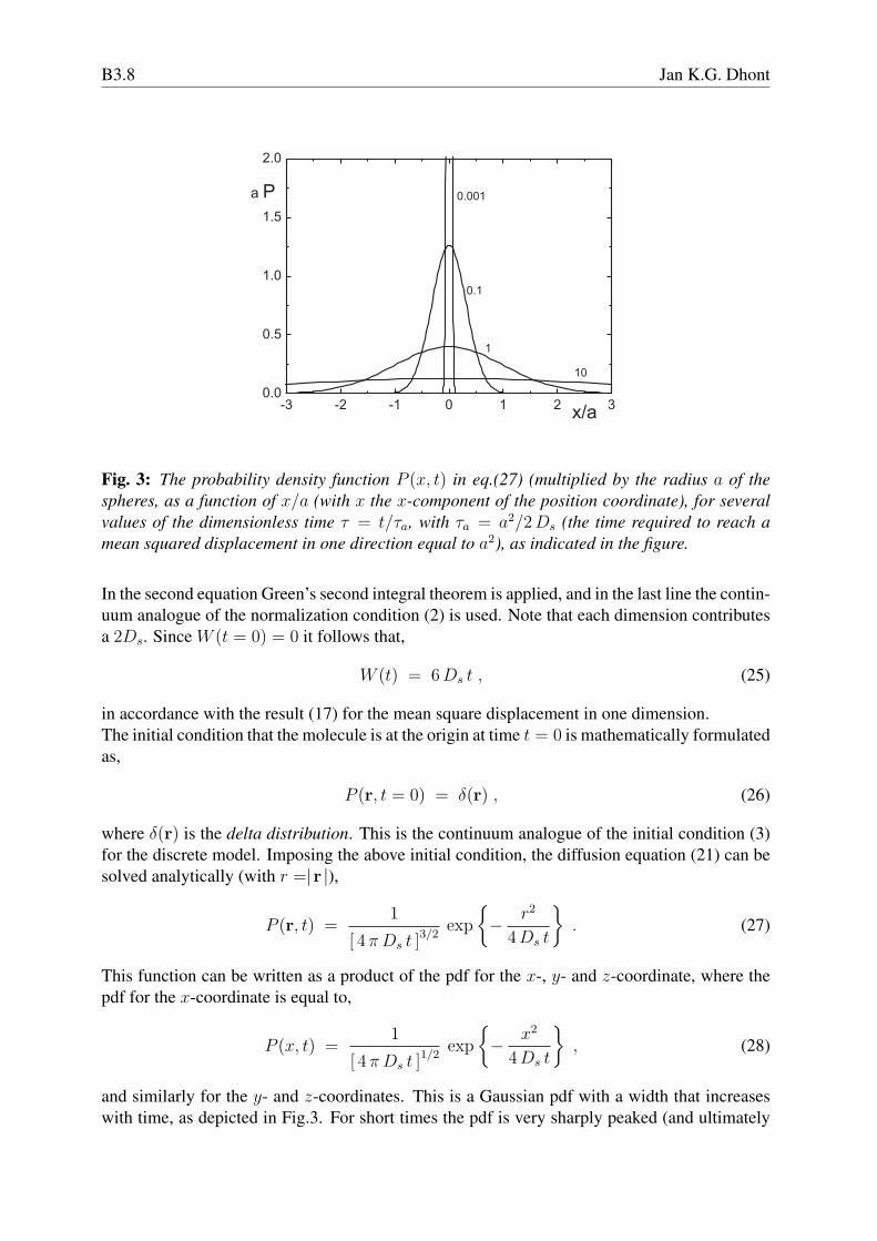
Fig. 3: The probability density function P (x, t) in eq.(27) (multiplied by the radius a of thespheres, as a function of x/a (with x the x-component of the position coordinate), for severalvalues of the dimensionless time τ = t/τa, with τa = a2/2 Ds (the time required to reach amean squared displacement in one direction equal to a2), as indicated in the figure.
In the second equation Green’s second integral theorem is applied, and in the last line the contin-uum analogue of the normalization condition (2) is used. Note that each dimension contributesa 2Ds. Since W (t = 0) = 0 it follows that,
W (t) = 6 Ds t , (25)
in accordance with the result (17) for the mean square displacement in one dimension.The initial condition that the molecule is at the origin at time t = 0 is mathematically formulatedas,
P (r, t = 0) = δ(r) , (26)
where δ(r) is the delta distribution. This is the continuum analogue of the initial condition (3)for the discrete model. Imposing the above initial condition, the diffusion equation (21) can besolved analytically (with r =|r |),
P (r, t) =1
[ 4 π Ds t ]3/2exp
{− r2
4 Ds t
}. (27)
This function can be written as a product of the pdf for the x-, y- and z-coordinate, where thepdf for the x-coordinate is equal to,
P (x, t) =1
[ 4 π Ds t ]1/2exp
{− x2
4 Ds t
}, (28)
and similarly for the y- and z-coordinates. This is a Gaussian pdf with a width that increaseswith time, as depicted in Fig.3. For short times the pdf is very sharply peaked (and ultimately
Diffusion B3.9
approaches the delta distribution as t → 0), while for larger times the probability for largedistances increases due to the diffusive displacement of the tracer molecule.The equation of motion (21) can be generalized to include an external force acting on themolecule. First notice that the probability P (r, t) can in principle be measured as follows. Amolecule that resides at the origin is released at time zero, after which its trajectory is recorded.This experiment is repeated many times. In each of the experiments, the molecule follows adifferent trajectory. The number of trajectories that intersect, at time t, a small box centered atr measures the pdf P (r, t). Alternatively, many non-interacting molecules can be released si-multaneously, and each of the trajectories is recorded. Since the molecules do not interact witheach other, they diffuse after release at time zero as if they were alone in the system. Each of themolecules thus exhibit self diffusion as described above. Again, the number of trajectories thatintersect a small box at r after a time t measures the pdf P (r, t). That number of trajectories,however, is also proportional to the local concentration ρ0(r, t) that one would measure (wherethe index ”0 ” refers to non-interacting molecules). We can thus interpret P (r, t) as the concen-tration ρ0(r, t) that exists when many non-interacting molecules are released at the origin r = 0at time t = 0. The number density obeys the exact continuity equation,
∂
∂tρ0(r, t) = −∇ · [ ρ0(r, t)v(r, t) ] , (29)
where v(r, t) is the thermally averaged velocity of molecules. When inertial forces are ne-glected (we shall comment on this at the end of this section), according to Newton’s equationof motion, there is a balance of forces, that is, all non-inertial forces add up to zero. Thereare three forces to be considered. First of all there is the friction force Ffr = −γ v that arisesfrom interactions of the molecule with surrounding matter, where γ is the friction coefficientthat was already introduced at the end of subsection 2.1. The second force is responsible for thevelocity that the molecule attains in the absence of an external force field, and is referred to asthe Brownian force FBr. The third force Fext is due to an external field. By force balance wehave,
Ffr + FBr + Fext = 0 → v =1
γ
[FBr + Fext
]. (30)
Substitution into eq.(29) and comparing with eq.(21), with P replaced by ρ0, in the absenceof an external field, leads to FBr = −γDs∇ ln{ ρ0(r, t) }. For a conservative force field, forwhich Fext = −∇Φ (with Φ the external potential), and in case equilibrium is reached, thedensity must be proportional to the Boltzmann exponential ρ0 ∼ exp {−Φ/kBT}. On the otherhand v = 0 in equilibrium, which immediately leads to γ Ds∇ ln{ρ0} +∇Φ = 0, and hence,ρ0 ∼ exp {−Φ/γ Ds}. It follows that Ds = kBT/γ, which reproduces the Einstein relation(18) that we found within the simple model considered in subsection 2.1. It also follows thatthe Brownian force is equal to,
FBr(r, t) = −kB T ∇ ln {ρ0(r, t)} , (31)
with ρ0 replaced by P (r, t) when used in the equation of motion for the pdf P (r, t). Using thisexpression for the Brownian force in eq.(29), and replacing the density ρ0 by the pdf P (r, t)thus leads to the generalization of the equation of motion eq.(21) to include an external forcefield,
∂
∂tP (r, t) = Ds∇ · [∇P (r, t)− β P (r, t)Fext(r)
]. (32)
B3.10 Jan K.G. Dhont
We will use this equation in the next subsection to calculate the self diffusion coefficient of amolecule in a prescribed energy landscape.In the above we assumed that inertial forces can be neglected. This is allowed on a time scalewhere the thermally averaged momentum coordinate, with a given initial value, relaxes to zero.According to Newton’s equation of motion, without an external field,
dp(t)
dt= − γ
mp(t) , (33)
where p = mv is the momentum coordinate and m is the mass of the molecule. It follows that(with p0 the initial momentum at time zero),
p(t) = p0 exp {− t/τ} , τ = m/γ . (34)
The time scale τ on which the momentum coordinate relaxes is very typically much smaller thanthe time during which appreciable diffusion occurs, which validates the neglect of inertia. Thetime scale on which inertial forces can be neglected is commonly referred to as the diffusivetime scale, while the dynamics on this time scale is referred to as overdamped dynamics.”overdamped” refers to the fact that friction forces are much larger than inertial forces.
2.3 Diffusion through a one-dimensional periodic energy landscapeAs an example of an explicit calculation of the self diffusion coefficient we consider a moleculethat interacts with its surroundings as described by a potential energy Φ. This potential isassumed to be periodic in one dimension, say the z-direction, and is constant along the othertwo directions : Φ ≡ Φ(z). An experimental example that will be discussed at the end of thissection is a rod-like molecule in a smectic phase that diffuses from one smectic layer to theother. The potential is assumed to be periodic with a period l, that is, Φ(z) = Φ(z + n l) forany integer n. We shall calculate the friction coefficient γ and employ the Einstein relationDs = kBT/γ to obtain the self diffusion coefficient in terms of the potential. In addition tothe force −∇Φ due to interactions with the surroundings, there is thus an additional appliedconstant force F app in the z-direction on the molecule that leads to a finite thermally averagedvelocity.For short times, the molecule ”rattles within potential valleys”. For longer times the moleculemoves from one valley to the other, that is, it moves across potential barriers. On can thereforedistinguish between a short-time self-diffusion coefficient that describes the thermal motionwithin a potential valley in the z-direction, and the long-time self diffusion coefficient thatdescribes thermal displacements between valleys. Here we calculate the long-time self diffusioncoefficient, which is relevant to mass transport on larger length scales.The long-time self diffusion coefficient can be calculated from an eigen-function expansion ofthe solution of the diffusion equation (32), with Fext ≡ −∇Φ + Fapp [1]. Alternatively, anexpression for the long-time self diffusion coefficient can be obtained without having to solvethe diffusion equation explicitly [2]. First of all, we identify the pdf P (x, t) as the concentrationof non-interacting molecules, an identification that has been discussed in subsection 2.2. Insteadof analyzing the motion of a single molecule under the action of the force Fapp, one can analyzethe motion of many non-interacting molecules simultaneously. Since the molecules do notinteract with each other, they move as if they were alone in the system, and hence they all movelike a self-diffuser. The stationary flux j0 of molecules in the x-direction is equal to (the indices
Diffusion B3.11
”0 ” refer to ”non-interacting molecules”),
j0 = ρ0(z) v(z) = ρ exp {−β Φ(z)} v(z) , (35)
where ρ is the number density that would have existed in the absence of the potential. Thisexpression is valid up to order (F app)2. The velocity is linear in F app, so that the zeroth-ordersolution for ρ0 ≡ P of eq.(32) with Fext ≡ −∇Φ can be used.Let τ be the mean time spend by a molecule within a valley. The mean velocity v can then beexpressed as (again, l is the periodicity of the potential),
v = l/τ . (36)
The number of molecules Nu within a single valley over an area A⊥ in the yz-plane is equal to,
Nu/A⊥ = j0 τ =
∫ l/2
−l/2
dz ρ0(z) = l ρ ≺ exp{−β Φ} Â , (37)
where the brackets define the periodicity average,
≺ f  ≡ 1
l
∫ l/2
−l/2
dz f(z) , (38)
for any function f(z). The last step in eq.(37) is valid up to leading order in F app. Note that j0
is linear in F app, while τ varies like 1/F app for sufficiently small applied forces, so that theirproduct is a constant to leading order.The force balance relation (30) for the present case reads,
F fr + F app − d
dz{ kBT ln ρ0 + Φ } = 0 . (39)
The local friction force F fr is equal to −γ0 v(z), where γ0 is the friction coefficient in theabsence of the potential Φ. On integration of both sides from z = −l/2 to +l/2, the gradientcontribution vanishes due to symmetry, and hence,
F app = γ01
l
∫ l/2
−l/2
dz v(z) . (40)
Combining the above equations we have,
1
l
∫ l/2
−l/2
dz v(z) =︸︷︷︸eq.(35)
j0
ρ≺ exp{+βΦ} Â
=︸︷︷︸eq.(37)
l
τ≺ exp{−βΦ} Â≺ exp{+βΦ} Â
=︸︷︷︸eq.(36)
v ≺ exp{−βΦ} Â≺ exp{+βΦ} Â . (41)
Hence, by substitution into eq.(40),
F app = γ v , with γ = γ0 ≺ exp{−βΦ} Â≺ exp{+βΦ} Â . (42)
B3.12 Jan K.G. Dhont
(a)
W(t) [micron /s]2
1.5
1.0
0.5
0
t [s]2.01.51.00.5
(c)(b)
potential/k TB
-0.5 0.50 1.0-1.0
0
1
2
3
z/L(a)(a)(a)
W(t) [micron /s]2
1.5
1.0
0.5
0
t [s]2.01.51.00.5
(c)
W(t) [micron /s]2
1.5
1.0
0.5
0
t [s]2.01.51.00.5
(c)(b)
potential/k TB
-0.5 0.50 1.0-1.0
0
1
2
3
z/L
(b)
potential/k TB
-0.5 0.50 1.0-1.0
0
1
2
3
z/L
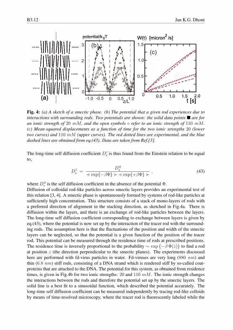
Fig. 4: (a) A sketch of a smectic phase. (b) The potential that a given rod experiences due tointeractions with surrounding rods. Two potentials are shown: the solid data points ¥ are foran ionic strength of 20 mM , and the open symbols ◦ refer to an ionic strength of 110 mM .(c) Mean-squared displacements as a function of time for the two ionic strengths 20 (lowertwo curves) and 110 mM (upper curves). The red dotted lines are experimental, and the bluedashed lines are obtained from eq.(43). Data are taken from Ref.[3].
The long-time self diffusion coefficient D ls is thus found from the Einstein relation to be equal
to,
D ls =
D 0s
≺ exp{−βΦ} Â≺ exp{+βΦ} Â , (43)
where D 0s is the self diffusion coefficient in the absence of the potential Φ.
Diffusion of colloidal rod-like particles across smectic layers provides an experimental test ofthis relation [3, 4]. A smectic phase is spontaneously formed by systems of rod-like particles atsufficiently high concentration. This structure consists of a stack of mono-layers of rods witha preferred direction of alignment in the stacking direction, as sketched in Fig.4a. There isdiffusion within the layers, and there is an exchange of rod-like particles between the layers.The long-time self diffusion coefficient corresponding to exchange between layers is given byeq.(43), where the potential is now set up by the interaction of the tracer rod with the surround-ing rods. The assumption here is that the fluctuations of the position and width of the smecticlayers can be neglected, so that the potential is a given function of the position of the tracerrod. This potential can be measured through the residence time of rods at prescribed positions.The residence time is inversely proportional to the probability ∼ exp {−β Φ(z)} to find a rodat position z (the direction perpendicular to the smectic planes). The experiments discussedhere are performed with fd-virus particles in water. Fd-viruses are very long (880 nm) andthin (6.8 nm) stiff rods, consisting of a DNA strand which is rendered stiff by so-called coat-proteins that are attached to the DNA. The potential for this system, as obtained from residencetimes, is given in Fig.4b for two ionic strengths: 20 and 110 mM . The ionic strength changesthe interactions between the rods and therefore the potential set up by the smectic layers. Thesolid line is a best fit to a sinusoidal function, which described the potential accurately. Thelong-time self diffusion coefficient can be measured independently by tracing rod-like colloidsby means of time-resolved microscopy, where the tracer rod is fluorescently labeled while the
Diffusion B3.13
0 5 100.0
0.5
1.0
80150200
500 nm
3 nm
Ds/D
0
[fd] mg/ml
210 nm
35 nm
mesh size [nm]
100
(c)
(a) (b)(a) (b)
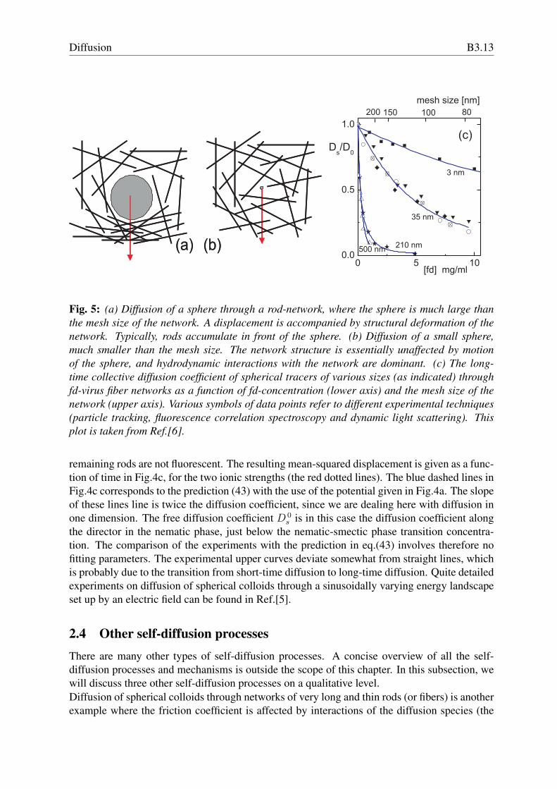
Fig. 5: (a) Diffusion of a sphere through a rod-network, where the sphere is much large thanthe mesh size of the network. A displacement is accompanied by structural deformation of thenetwork. Typically, rods accumulate in front of the sphere. (b) Diffusion of a small sphere,much smaller than the mesh size. The network structure is essentially unaffected by motionof the sphere, and hydrodynamic interactions with the network are dominant. (c) The long-time collective diffusion coefficient of spherical tracers of various sizes (as indicated) throughfd-virus fiber networks as a function of fd-concentration (lower axis) and the mesh size of thenetwork (upper axis). Various symbols of data points refer to different experimental techniques(particle tracking, fluorescence correlation spectroscopy and dynamic light scattering). Thisplot is taken from Ref.[6].
remaining rods are not fluorescent. The resulting mean-squared displacement is given as a func-tion of time in Fig.4c, for the two ionic strengths (the red dotted lines). The blue dashed lines inFig.4c corresponds to the prediction (43) with the use of the potential given in Fig.4a. The slopeof these lines line is twice the diffusion coefficient, since we are dealing here with diffusion inone dimension. The free diffusion coefficient D 0
s is in this case the diffusion coefficient alongthe director in the nematic phase, just below the nematic-smectic phase transition concentra-tion. The comparison of the experiments with the prediction in eq.(43) involves therefore nofitting parameters. The experimental upper curves deviate somewhat from straight lines, whichis probably due to the transition from short-time diffusion to long-time diffusion. Quite detailedexperiments on diffusion of spherical colloids through a sinusoidally varying energy landscapeset up by an electric field can be found in Ref.[5].
2.4 Other self-diffusion processesThere are many other types of self-diffusion processes. A concise overview of all the self-diffusion processes and mechanisms is outside the scope of this chapter. In this subsection, wewill discuss three other self-diffusion processes on a qualitative level.Diffusion of spherical colloids through networks of very long and thin rods (or fibers) is anotherexample where the friction coefficient is affected by interactions of the diffusion species (the
B3.14 Jan K.G. Dhont
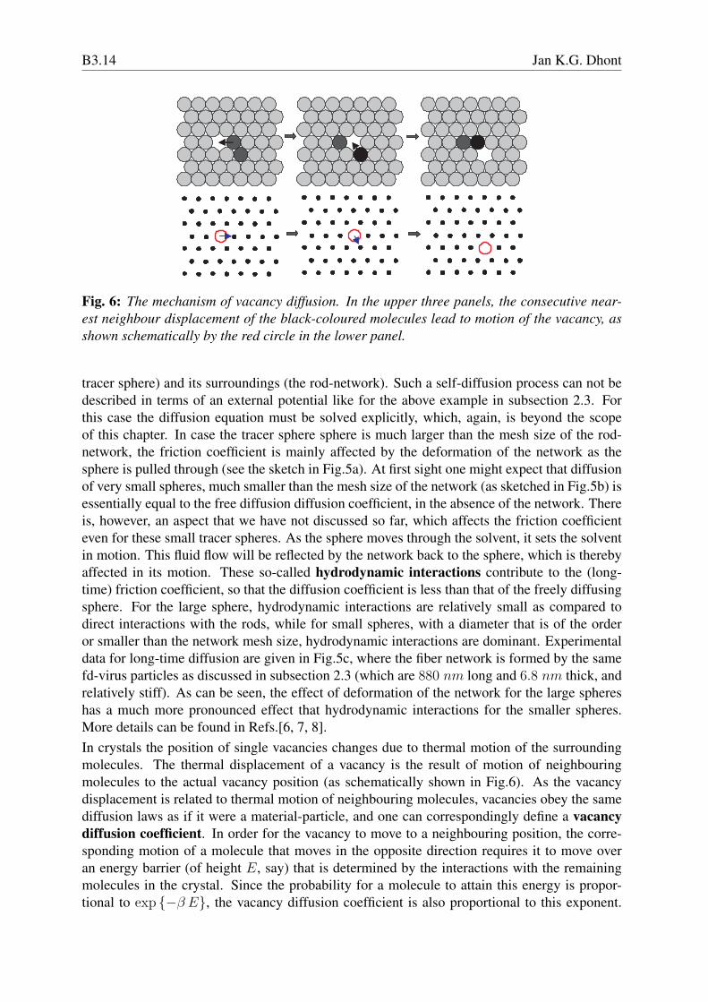
Fig. 6: The mechanism of vacancy diffusion. In the upper three panels, the consecutive near-est neighbour displacement of the black-coloured molecules lead to motion of the vacancy, asshown schematically by the red circle in the lower panel.
tracer sphere) and its surroundings (the rod-network). Such a self-diffusion process can not bedescribed in terms of an external potential like for the above example in subsection 2.3. Forthis case the diffusion equation must be solved explicitly, which, again, is beyond the scopeof this chapter. In case the tracer sphere sphere is much larger than the mesh size of the rod-network, the friction coefficient is mainly affected by the deformation of the network as thesphere is pulled through (see the sketch in Fig.5a). At first sight one might expect that diffusionof very small spheres, much smaller than the mesh size of the network (as sketched in Fig.5b) isessentially equal to the free diffusion diffusion coefficient, in the absence of the network. Thereis, however, an aspect that we have not discussed so far, which affects the friction coefficienteven for these small tracer spheres. As the sphere moves through the solvent, it sets the solventin motion. This fluid flow will be reflected by the network back to the sphere, which is therebyaffected in its motion. These so-called hydrodynamic interactions contribute to the (long-time) friction coefficient, so that the diffusion coefficient is less than that of the freely diffusingsphere. For the large sphere, hydrodynamic interactions are relatively small as compared todirect interactions with the rods, while for small spheres, with a diameter that is of the orderor smaller than the network mesh size, hydrodynamic interactions are dominant. Experimentaldata for long-time diffusion are given in Fig.5c, where the fiber network is formed by the samefd-virus particles as discussed in subsection 2.3 (which are 880 nm long and 6.8 nm thick, andrelatively stiff). As can be seen, the effect of deformation of the network for the large sphereshas a much more pronounced effect that hydrodynamic interactions for the smaller spheres.More details can be found in Refs.[6, 7, 8].In crystals the position of single vacancies changes due to thermal motion of the surroundingmolecules. The thermal displacement of a vacancy is the result of motion of neighbouringmolecules to the actual vacancy position (as schematically shown in Fig.6). As the vacancydisplacement is related to thermal motion of neighbouring molecules, vacancies obey the samediffusion laws as if it were a material-particle, and one can correspondingly define a vacancydiffusion coefficient. In order for the vacancy to move to a neighbouring position, the corre-sponding motion of a molecule that moves in the opposite direction requires it to move overan energy barrier (of height E, say) that is determined by the interactions with the remainingmolecules in the crystal. Since the probability for a molecule to attain this energy is propor-tional to exp {−β E}, the vacancy diffusion coefficient is also proportional to this exponent.
Diffusion B3.15
(a) (b) (c) (d)(a) (b) (c) (d)
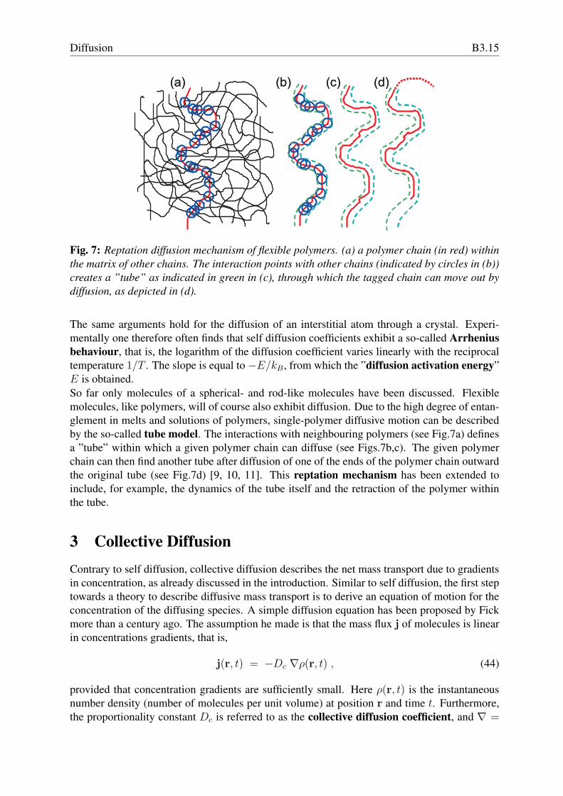
Fig. 7: Reptation diffusion mechanism of flexible polymers. (a) a polymer chain (in red) withinthe matrix of other chains. The interaction points with other chains (indicated by circles in (b))creates a ”tube” as indicated in green in (c), through which the tagged chain can move out bydiffusion, as depicted in (d).
The same arguments hold for the diffusion of an interstitial atom through a crystal. Experi-mentally one therefore often finds that self diffusion coefficients exhibit a so-called Arrheniusbehaviour, that is, the logarithm of the diffusion coefficient varies linearly with the reciprocaltemperature 1/T . The slope is equal to −E/kB, from which the ”diffusion activation energy”E is obtained.So far only molecules of a spherical- and rod-like molecules have been discussed. Flexiblemolecules, like polymers, will of course also exhibit diffusion. Due to the high degree of entan-glement in melts and solutions of polymers, single-polymer diffusive motion can be describedby the so-called tube model. The interactions with neighbouring polymers (see Fig.7a) definesa ”tube” within which a given polymer chain can diffuse (see Figs.7b,c). The given polymerchain can then find another tube after diffusion of one of the ends of the polymer chain outwardthe original tube (see Fig.7d) [9, 10, 11]. This reptation mechanism has been extended toinclude, for example, the dynamics of the tube itself and the retraction of the polymer withinthe tube.
3 Collective DiffusionContrary to self diffusion, collective diffusion describes the net mass transport due to gradientsin concentration, as already discussed in the introduction. Similar to self diffusion, the first steptowards a theory to describe diffusive mass transport is to derive an equation of motion for theconcentration of the diffusing species. A simple diffusion equation has been proposed by Fickmore than a century ago. The assumption he made is that the mass flux j of molecules is linearin concentrations gradients, that is,
j(r, t) = −Dc ∇ρ(r, t) , (44)
provided that concentration gradients are sufficiently small. Here ρ(r, t) is the instantaneousnumber density (number of molecules per unit volume) at position r and time t. Furthermore,the proportionality constant Dc is referred to as the collective diffusion coefficient, and ∇ =
B3.16 Jan K.G. Dhont
(∂/∂x, ∂/∂y, ∂/∂z) is the nabla- or gradient-operator. A minus sign is added to the right hand-side in eq.(44) to render Dc positive (note that the flux is typically directed towards regions oflow concentration, as already discussed in the introduction). Substitution of this expression forthe flux into the continuity equation gives,
In concentrated systems, the collective diffusion coefficient depends on concentration, Dc ≡Dc(ρ(r, t)), so that it can not placed in front of the ∇− operator. Suppose, however, that thedeviation of the density from its average value is small. That is, ρ(r, t) = ρ + δρ(r, t), withδρ(r, t)/ρ ¿ 1, where ρ is the number density of the system without concentration gradients.When this is assumed, the diffusion equation (45) can be written, up to linear order in δρ(r, t),as,
∂ρ(r, t)
∂t= Dc∇2ρ(r, t) , (46)
The assumption of small overall deviations from the average density is a quite severe assumptionthat is not satisfied for many cases, so that eq.(45) is relevant rather than eq.(46). For very dilutesystems, where inter-molecular interactions are absent, this is a valid procedure, since then Dc
is indeed a constant. In that case eq(46) reproduces eq.(21) for self diffusion (as discussed insubsection 2.2, this equation also holds for the concentration when interactions between thetracer molecules are absent). It follows that, for very dilute system, the self- and collectivediffusion coefficients are identical,
D0s = D0
c , (47)
where the superscript ”0 ” is used to indicate that interactions between diffusing species areabsent. In most practical systems, the concentration of diffusing molecules is large, such thatinter-molecular interactions are important for the diffusive properties. The collective diffusioncoefficient under such conditions is different from D0
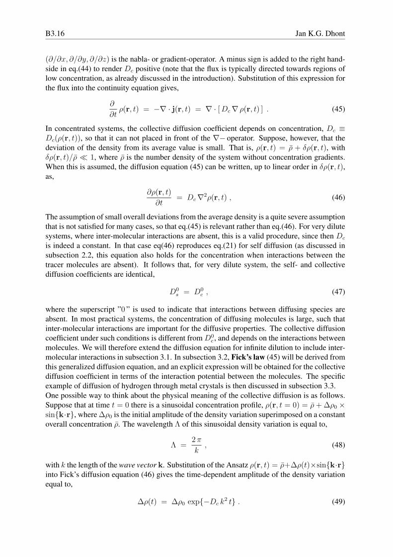
c , and depends on the interactions betweenmolecules. We will therefore extend the diffusion equation for infinite dilution to include inter-molecular interactions in subsection 3.1. In subsection 3.2, Fick’s law (45) will be derived fromthis generalized diffusion equation, and an explicit expression will be obtained for the collectivediffusion coefficient in terms of the interaction potential between the molecules. The specificexample of diffusion of hydrogen through metal crystals is then discussed in subsection 3.3.One possible way to think about the physical meaning of the collective diffusion is as follows.Suppose that at time t = 0 there is a sinusoidal concentration profile, ρ(r, t = 0) = ρ + ∆ρ0 ×sin{k·r}, where ∆ρ0 is the initial amplitude of the density variation superimposed on a constantoverall concentration ρ. The wavelength Λ of this sinusoidal density variation is equal to,
Λ =2 π
k, (48)
with k the length of the wave vector k. Substitution of the Ansatz ρ(r, t) = ρ+∆ρ(t)×sin{k·r}into Fick’s diffusion equation (46) gives the time-dependent amplitude of the density variationequal to,
∆ρ(t) = ∆ρ0 exp{−Dc k2 t} . (49)
Diffusion B3.17
The collective diffusion coefficient thus determines how fast a sinusoidal concentration profilerelaxes. The relaxation rate varies with the wavelength as ∼ Λ−2, the interpretation of which isthat it takes particles longer to diffuse over longer distances, while the time it takes to diffuseover a certain distance is quadratically depending on that distance (as quantified by eq.(25) forthe mean-squared displacement of a single particle). As will be seen in the next subsection,the validity of eq.(46) (and hence of eq.(49)) is limited to wavelengths that are much largerthan the range of the pair-interaction potential between the diffusing particles. When the pair-interactions between particles is repulsive, it is intuitively obvious that the particles in regionsof high concentration are pushed apart more strongly at higher overall concentrations ρ, whichleads to a faster relaxation. In other words, the collective diffusion coefficient is expected toincrease with increasing overall concentration. For the same reason a decrease is expectedfor particles with attractive pair-interaction potentials. The above intuitive arguments are onlyvalid for sufficiently low concentrations ρ, such that interactions between two given particlesis not too much affected by the presence of other particles. At sufficiently high concentrations,the collective diffusion coefficient can decrease with increasing concentration ρ due to indi-rect interactions at large overall concentrations also for repulsive pair-interactions potentials.In addition to direct interactions, also hydrodynamic interactions can play an important role inthe concentration dependence of the collective diffusion coefficient of particles in a solvent. Amoving particle in a solvent induces a fluid flow that affects other particles in their motion, andtherefore the value of the collective diffusion coefficient. Such hydrodynamic interactions willnot be discussed in this chapter (more about the concentration dependence of diffusion coef-ficients of spherical particles in a solvent and hydrodynamic interactions can be found in, forexample, Ref.[12, 13, 14]). While the collective diffusion coefficient increases with concentra-tion in case of repulsive interactions, it is obvious that the self diffusion coefficient decreases.Due to the repulsive interactions with neighbouring particles, the diffusive displacement of agiven particle is hindered, leading to a decrease of the mean-squared displacement, and thus toa smaller self diffusion coefficient.Attractive interactions between particles can be so strong, that it is energetically favorable to in-crease an initial inhomogeneity. According to eq.(49) this happens when the collective diffusioncoefficient is negative. A homogeneous system with a negative collective diffusion coefficientis unstable in the sense that arbitrary small fluctuations in the concentration leads to the for-mation of inhomogeneities. Such a growth of inhomogeneities, that ultimately leads completephase separation, is referred to as spinodal decomposition. Spinodal decomposition will bediscussed in some detail in section 4.
3.1 A generalized diffusion equationAs discussed at the end of subsection 2.2, there is force balance in the overdamped limit (orequivalently, on the diffusive time scale). Since inertial forces can be neglected, all other forcesadd up to zero on the diffusive time scale. In the dilute limit, where interactions betweenmolecules can be neglected, force balance results in the expression (30) for the velocity of agiven molecule, with the Brownian force being given in eq.(31) (where the number density isnow denoted as ρ, without the subscript ”0 ”, since we here consider the more general case ofconcentrated systems). For interacting molecules, at relatively high concentration, the externalforce in eq.(30) is equal to the force that acts on a given molecule due to interactions withneighbouring molecules. We will denote this force by FI instead of Fext, to indicate that theforce is now due to inter-molecular interactions.
B3.18 Jan K.G. Dhont
The force FI on a molecule at r due to the presence of a second molecule at r′ is equal to−∇V (| r − r′ |), with V the pair-interaction potential. The force experienced by the moleculeat r is equal to this pair-force, multiplied by the number of neighbouring molecules around thegive molecule at position r, averaged over all positions r′ of neighbouring molecules,
FI(r, t) = −∫
dr′ g(r, r′, t) ρ(r′, t)∇V (|r− r′ |) , (50)
where g(r, r′, t) is the probability to find a molecule at r′, given that there is a molecule at r.This conditional probability density function is commonly referred to as the pair-correlationfunction. From the above mentioned force balance, we have, γ0 v = FBr + FI , where γ0 isthe friction coefficient at infinite dilution, that is, in the absence of inter-molecular interactions.The corresponding flux j = ρv is thus equal to,
j(r, t) = −D0c
[∇ρ(r, t) + β ρ(r, t)
∫dr′ g(r, r′, t) ρ(r′, t)∇V (|r− r′ |)
], (51)
where, as before, β = 1/kBT and D0c = kBT/γ0. This expression for the flux can be substituted
into the exact conservation equation, to obtain a generalized diffusion equation,
∂ρ(r, t)
∂t= −∇ · j(r, t)
= D0c
[∇2ρ(r, t) + β∇ ·
{ρ(r, t)
∫dr′ g(r, r′, t) ρ(r′, t)∇V (|r− r′ |)
}]. (52)
This is the fundamental equation of motion that will be used in the sequel to analyze the collec-tive diffusion at finite concentrations.
3.2 Derivation of Fick’s law for concentrated systems
The generalized diffusion equation (52) can be used to derive Fick’s law (45), where an ex-plicit expression will be obtained for the collective diffusion coefficient Dc in terms of thepair-interaction potential V . The linear relationship (44) between the mass flux and spatial gra-dients in the concentration is expected to hold only for sufficiently small gradients. We willtherefore assume that on the distance RV over which the pair-potential V falls off to zero, thedensity is essentially a linear function of position. The following Taylor expansion can thus beused in the integral in eq.(52) (with R = r
′−r,),
ρ(r′, t) ≈ ρ(r, t) + R · ∇ρ(r, t) , (53)
since the pair-potential limits the integration range in r′-space to a region of extent RV around
r. Here the ”· ” is the inner product of the two vectors on both sides. An appropriate ap-proximation for the pair-correlation function can be obtained as follows. First of all, we needan approximation only for | r − r
′ |≤ RV . For such small, microscopic distances, the pair-correlation function relaxes essentially instantaneous to equilibrium relative to the time scaleon which the concentration evolves. We can therefore take the pair-correlation function equalto its equilibrium value geq. This approximation can be considered as a statistical mechanicalanalogue of the thermodynamic local equilibrium assumption that is made in the theory of
Diffusion B3.19
irreversible thermodynamics. A natural choice is to take this equilibrium function equal to thatof a homogenous system with a density in between the points r and r
′ ,
g(r, r′, t) ≈ geq(|r− r
′ |) , ρ ≡ ρ
(r + r
′
2, t
). (54)
Note that due to translational and rotational invariance of a homogeneous system, the pair-correlation function depends on r and r,′ only through | r − r
′ |. Thus, again Tayloring up tolinear spatial dependencies, after writing (r + r
′)/2 as r + 1
2 R,
g(r, r′, t) ≈ geq(R) +
{ρ
(r + r
′
2, t
)− ρ(r, t)
}d
dρgeq(R)
≈ geq(R) + 12
dgeq(R)
dρR · ∇ρ(r, t) , (55)
where geq(R, t) is the equilibrium pair-correlation function for a homogeneous system withconcentration ρ(r, t), which is thus an implicit function of r and t, and the density derivativeis with respect to ρ(r, t). This implicit dependence is not denoted here explicitly for brevity.Substitution of the expansions (53,55) into the integral in eq.(52), using that ∇V (| r − r
′ |) =−R dV (R)/dR (with R = R/R the unit vector along R), together with,∮
dR R = 0 ,∮
dR R R =4π
3I , (56)
where the integrals range over all directions of R, and I is the identity tensor, leads to,
ρ(r, t)
∫dr′ g(r, r′, t) ρ(r′, t)∇V (|r− r′ |) =
2π
3∇ρ
d
dρ
[ρ2
∫ ∞
0
dR R3 dV (R)
dRgeq(R)
]. (57)
We can now employ the standard equilibrium statistical mechanical expression for the pressureP eq,
P eq = ρ kBT − 2π
3ρ2
∫ ∞
0
dR R3 dV (R)
dRgeq(R) , (58)
to obtain Fick’s diffusion equation (45) with,
Dc(ρ(r, t)) ≡ D0c β
dP eq(ρ(r, t))
dρ(r, t). (59)
When gradients in concentrations are very large, such that the concentrations varies non-linearlyon length scales set by the range RV of the inter-molecular pair-potential, the Taylor expansions(53,55) are inaccurate, and higher orders of ∇ come into play in the diffusion equation.Note that (dP eq/dρ) ∇ρ = ∇P eq, which suggests that mass transport is driven by gradients inthe pressure, which is intuitively appealing.There is a subtlety for solutions of macromolecules. Instead of the mechanical pressure, theosmotic pressure appears in eq.(59) for the diffusion coefficient. This is a consequence of thefact that the macro-molecular pair-correlation function is thermally averaged with respect tothe degrees of freedom of the solvent molecules. Furthermore, we neglected hydrodynamicinteractions between such macromolecules, which do have an effect on the diffusive properties.A detailed discussion of these facts is beyond the scope of this chapter. The full expressionfor the diffusion coefficient of spherical macromolecules in solution, including the effects ofhydrodynamic interactions, can be found in, for example, Ref.[12, 13, 14].
B3.20 Jan K.G. Dhont
3.3 Diffusion of hydrogen through metals
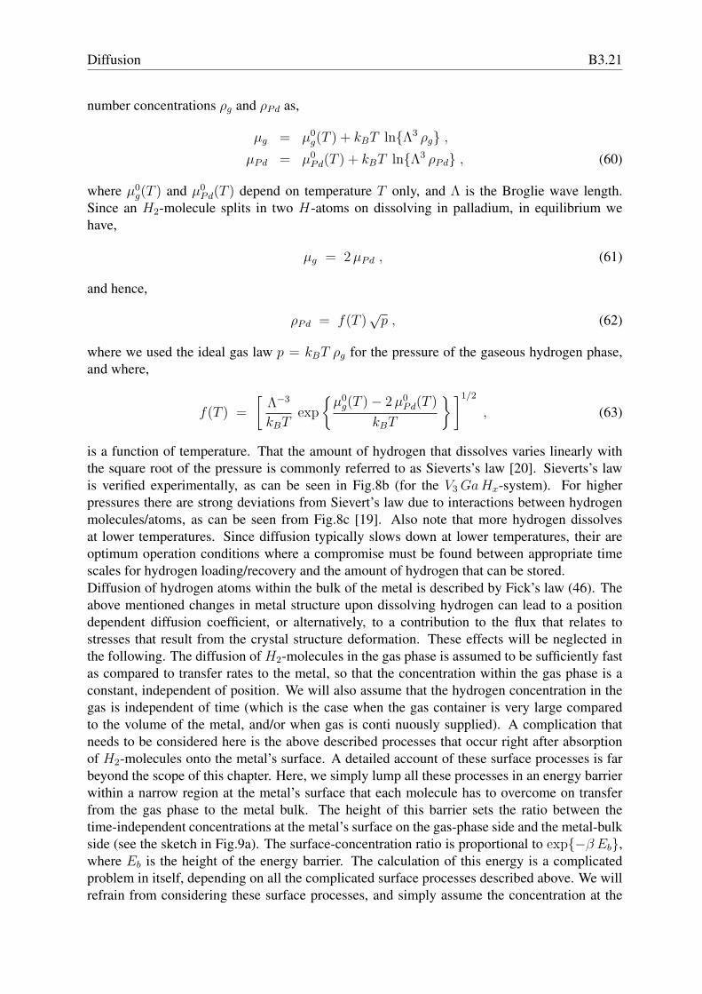
Diffusion of hydrogen through metals has been studied since about 1850, and revived as a re-search area some decades ago due to the possible applications in energy storage. Hydrogendissolves in metals not as intact H2-molecules but as H-atoms, which reside at interstitial po-sitions of the metal’s crystal structure. There is a large number of neighbouring interstitialpositions, so that hydrogen diffuses much faster as compared to diffusion of a molecule, wherea thermal displacement requires the improbable event that there is a neighbouring vacancy (amissing atom in the crystal) to which it can move to. Fast diffusion of hydrogen is important forpossible energy storage, since hydrogen must be dissolved in the metal (upon storage) and re-moved from the metal (upon use) within a reasonable time. Other important aspects for energystorage are the amount of hydrogen that can be dissolved, the effect of the mechanical prop-erties of the metal on dissolving hydrogen, and the processes that occur right after absorptionof hydrogen at the metal’s surface, One of the metals in which large amounts of hydrogen canbe dissolved is palladium. This is also one of the few metals that do not brittle and keeps to alarge extent its original structural properties upon dissolving large amounts of hydrogen. Wewill therefore mainly focus on palladium. Right after absorption of hydrogen on the metal’ssurface, diffusion into the metal first requires the dissociation of H2 into H-atoms, followedby surface diffusion of the atoms in order to find the appropriate locations to enter the metalcrystal, after which diffusion into the bulk of the metal occurs. Dissolving hydrogen changesthe lattice spacing of the crystal, mechanical stresses and crystal defects may be created, whichboth affect the diffusive properties of the H-atoms. Needless to say that a detailed discussionof all these complications can not be covered in this section. In the following we will brieflydiscuss the most important features of hydrogen-metal systems, and discuss diffusion from thegas phase into the metal on the basis of a simple diffusion model that accounts for crossingthe surface of the metal. Besides transferring hydrogen into a metal by exposure to hydrogengas, other methods can be used, like electrochemical deposition or by partially ionizing the gasphase, which circumvent the necessary dissociation after absorption to the metal’s surface.Let us first consider the phase behaviour of the hydrogen/palladium system. For low concentra-tions of hydrogen, it is homogeneously distributed within the palladium. For large concentra-tions, and sufficiently low temperatures, where the H-atoms strongly interact (through the crys-tal environment), phase separation is observed where a H-rich phase coexists with a H-poorphase. In both phases the hydrogen is disordered,while at room temperature the crystal latticespacing for the H-poor phase is 0.3894 nm, and for the H-rich phase 0.4040 nm [15, 16]. Itseems likely that this phase equilibrium is similar to a gas-liquid phase coexistence, where ”thegas” is the H-poor phase, and ”the liquid” is the H-rich phase. The only difference between thetwo phases is their hydrogen concentration (and the difference lattice spacing of the palladiumcrystal), without any structural differences, like for a gas and a liquid. The experimental phasediagram is shown in Fig.8a [17, 18]. The line is the binodal, which has much the same formas for common gas-liquid coexistence. Notice that large amounts of hydrogen can be solved inpalladium, where the ratio of hydrogen to palladium atoms is close to unity.The simplest way to dissolve hydrogen in metals (palladium in particular), is by exposing themetal to gaseous hydrogen, of which the pressure can be varied by external means. Typically,more hydrogen dissolves when the hydrogen pressure is increased. First consider small pres-sures, such that H2-molecules in the gaseous phase and H-atoms in the palladium environmentdo not interact with each other. For such ideal systems the chemical potential µg and µPd ofhydrogen in the gaseous phase and in palladium, respectively, depend on the corresponding
Diffusion B3.21
number concentrations ρg and ρPd as,
µg = µ0g(T ) + kBT ln{Λ3 ρg} ,
µPd = µ0Pd(T ) + kBT ln{Λ3 ρPd} , (60)
where µ0g(T ) and µ0
Pd(T ) depend on temperature T only, and Λ is the Broglie wave length.Since an H2-molecule splits in two H-atoms on dissolving in palladium, in equilibrium wehave,
µg = 2 µPd , (61)
and hence,
ρPd = f(T )√
p , (62)
where we used the ideal gas law p = kBT ρg for the pressure of the gaseous hydrogen phase,and where,
f(T ) =
[Λ−3
kBTexp
{µ0
g(T )− 2 µ0Pd(T )
kBT
}]1/2
, (63)
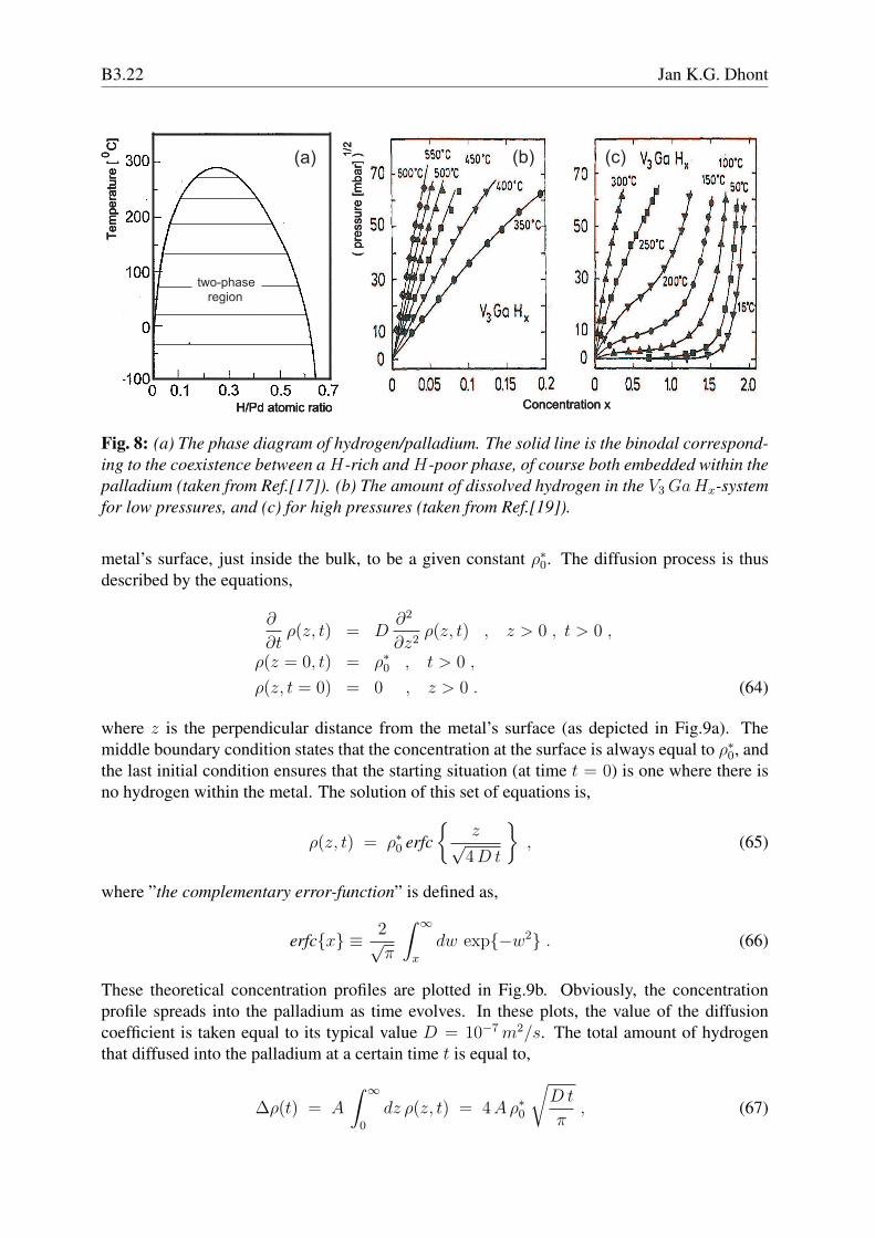
is a function of temperature. That the amount of hydrogen that dissolves varies linearly withthe square root of the pressure is commonly referred to as Sieverts’s law [20]. Sieverts’s lawis verified experimentally, as can be seen in Fig.8b (for the V3 GaHx-system). For higherpressures there are strong deviations from Sievert’s law due to interactions between hydrogenmolecules/atoms, as can be seen from Fig.8c [19]. Also note that more hydrogen dissolvesat lower temperatures. Since diffusion typically slows down at lower temperatures, their areoptimum operation conditions where a compromise must be found between appropriate timescales for hydrogen loading/recovery and the amount of hydrogen that can be stored.Diffusion of hydrogen atoms within the bulk of the metal is described by Fick’s law (46). Theabove mentioned changes in metal structure upon dissolving hydrogen can lead to a positiondependent diffusion coefficient, or alternatively, to a contribution to the flux that relates tostresses that result from the crystal structure deformation. These effects will be neglected inthe following. The diffusion of H2-molecules in the gas phase is assumed to be sufficiently fastas compared to transfer rates to the metal, so that the concentration within the gas phase is aconstant, independent of position. We will also assume that the hydrogen concentration in thegas is independent of time (which is the case when the gas container is very large comparedto the volume of the metal, and/or when gas is conti nuously supplied). A complication thatneeds to be considered here is the above described processes that occur right after absorptionof H2-molecules onto the metal’s surface. A detailed account of these surface processes is farbeyond the scope of this chapter. Here, we simply lump all these processes in an energy barrierwithin a narrow region at the metal’s surface that each molecule has to overcome on transferfrom the gas phase to the metal bulk. The height of this barrier sets the ratio between thetime-independent concentrations at the metal’s surface on the gas-phase side and the metal-bulkside (see the sketch in Fig.9a). The surface-concentration ratio is proportional to exp{−β Eb},where Eb is the height of the energy barrier. The calculation of this energy is a complicatedproblem in itself, depending on all the complicated surface processes described above. We willrefrain from considering these surface processes, and simply assume the concentration at the
B3.22 Jan K.G. Dhont
H/Pd atomic ratio
Tem
pera
ture
[C
]0
two-phaseregion
(a)
H/Pd atomic ratio
Tem
pera
ture
[C
]0
two-phaseregion
(a)
H/Pd atomic ratio
Tem
pera
ture
[C
]0
two-phaseregion
H/Pd atomic ratio
Tem
pera
ture
[C
]0
two-phaseregion
(a)
Concentration x
(pre
ssure
[mbar]
)1/2
(b) (c)
Concentration x
(pre
ssure
[mbar]
)1/2
Concentration x
(pre
ssure
[mbar]
)1/2
(b) (c)
Fig. 8: (a) The phase diagram of hydrogen/palladium. The solid line is the binodal correspond-ing to the coexistence between a H-rich and H-poor phase, of course both embedded within thepalladium (taken from Ref.[17]). (b) The amount of dissolved hydrogen in the V3 GaHx-systemfor low pressures, and (c) for high pressures (taken from Ref.[19]).
metal’s surface, just inside the bulk, to be a given constant ρ∗0. The diffusion process is thusdescribed by the equations,
∂
∂tρ(z, t) = D
∂2
∂z2ρ(z, t) , z > 0 , t > 0 ,
ρ(z = 0, t) = ρ∗0 , t > 0 ,
ρ(z, t = 0) = 0 , z > 0 . (64)
where z is the perpendicular distance from the metal’s surface (as depicted in Fig.9a). Themiddle boundary condition states that the concentration at the surface is always equal to ρ∗0, andthe last initial condition ensures that the starting situation (at time t = 0) is one where there isno hydrogen within the metal. The solution of this set of equations is,
ρ(z, t) = ρ∗0 erfc{
z√4 D t
}, (65)
where ”the complementary error-function” is defined as,
erfc{x} ≡ 2√π
∫ ∞
x
dw exp{−w2} . (66)
These theoretical concentration profiles are plotted in Fig.9b. Obviously, the concentrationprofile spreads into the palladium as time evolves. In these plots, the value of the diffusioncoefficient is taken equal to its typical value D = 10−7 m2/s. The total amount of hydrogenthat diffused into the palladium at a certain time t is equal to,
∆ρ(t) = A
∫ ∞
0
dz ρ(z, t) = 4 Aρ∗0
√D t
π, (67)
Diffusion B3.23
gaseous
hydrogen
H2
energy
position z
palladium
H
Eb
z=0
(a)
gaseous
hydrogen
H2
energy
position z
palladium
H
Eb
z=0
(a)
Pressure [bar]
Diffu
sio
nco
eff
icie
nt[c
m/s
]2
Ds
Dc
(c)
10-4
10-3
10-2
Pressure [bar]
Diffu
sio
nco
eff
icie
nt[c
m/s
]2
Ds
Dc
(c)
10-4
10-3
10-2
0.00 0.01 0.020.00
0.25
0.50
0.75
1.00
t=10000 seconds
1000
100
1
r/r0
z [m]
10
*
(b)
Fig. 9: (a) A sketch of the simplified model for the kinetics of transfer of hydrogen from the gasphase to the metal bulk. (b) The concentration profiles (ρ/ρ∗0 versus z) for different times, ac-cording to eqs.(65,66) The value of the diffusion coefficient is taken equal to D = 10−7 m2/s.(c) The self- and collective diffusion coefficients of hydrogen in Zn(bdc)(ted)0.5, bdc = ben-zenedicarboxylate, ted = triethylenediamine (taken from Ref.[21]).
where A is the area of the surface that is exposed to the hydrogen gas. The amount of storedhydrogen thus saturates as the square root of time. Typically, a palladium with a surface area ofA = 1 m2 stores within an hour about 0.04 × ρ∗0[m
−3] hydrogen atoms. A reasonable estimatefor ρ∗0 is a typical concentration in equilibrium, which is of the order 1027 H− atoms/m3. Thisgives an amount of hydrogen stored in one hour equal to about 100 gram. It is questionablewhether this slow storage rate justifies an economic application, also in view of the high priceof palladium [I am, however, hesitant to make a statement like this since my knowledge ofeconomy is essentially equal to zero].
Both the self- and collective diffusion coefficients of hydrogen atoms are concentration depen-dent as a result of mutual interactions. This can be seen in Fig.9c, where both coefficients areplotted as a function the pressure of the gas phase for a certain metallic compound [21]. Asexplained in the introduction to section 3, the expected increase of the collective diffusion coef-ficient and the decrease of the self diffusion coefficient in case of repulsive H −H interactionswith increasing concentration is indeed observed. For larger concentrations of hydrogen andsufficiently low temperatures, however, attractions between H-atoms must be present since agas-liquid phase separation is observed, as discussed above. Since gas-liquid phase transitionsare abundant and occur in many different types of systems, the next section is devoted to thekinetics of gas-liquid phase separation from an initially unstable state, which is referred to asspinodal decomposition.
Solutions of Fick’s diffusion equation for many types of geometries (like the infinite half-planegeometry in the above example) are discussed in Ref.[22].
B3.24 Jan K.G. Dhont
4 A Negative Diffusion Coefficient: Spinodal DecompositionAs already mentioned at the end of the introduction to section 3, the collective diffusion coef-ficient can become negative when strong attractions between the molecules exist. This leads toa temporal increase of inhomogeneities (which are always present due to fluctuations) and ulti-mately leads to full phase separation. According to eq.(59) the collective diffusion coefficient isnegative when dP eq/dρ < 0 (with P eq the equilibrium pressure of the homogeneous system andρ the number density of the homogeneous system). The pressure thus decreases with increasingconcentration, which is counter intuitive, and therefore hints to an instability. The kinetics ofphase separation starting from an homogeneous, unstable system is referred to as spinodal de-composition. Phase separation from an initially meta-stable system, where nuclei are formedthat grow in time, is referred to as nucleation-and growth. As will be seen in this section,the initial morphology in case of spinodal decomposition is qualitatively different from nucle-ation and growth. Instead of more-or-less ad-random distributed small nuclei of a significantlydifferent concentration as compared to the initially homogeneous system, during spinodal de-composition a continuous growth of density differences is observed, where the relatively lowand high concentration regions form a bi-continuous, space-spanning labyrinth structure.The aim of this section is to quantitatively describe the temporal evolution of the density duringthe initial stages of phase separation of an unstable, initially homogeneous state. The pointof departure is the generalized diffusion equation (52). This approach can be considered asthe microscopic foundation of the classic Cahn-Hilliard theory of spinodal decomposition,which is based on irreversible thermodynamics [23, 24, 25].
4.1 An introduction to spinodal decomposition
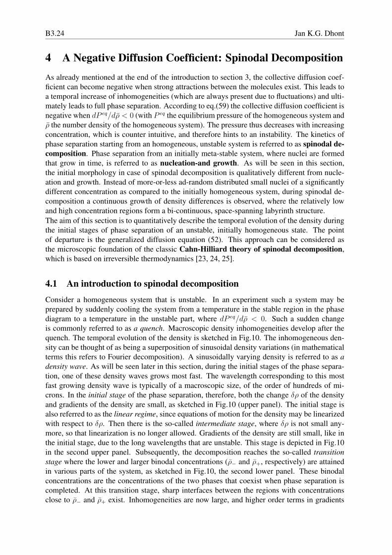
Consider a homogeneous system that is unstable. In an experiment such a system may beprepared by suddenly cooling the system from a temperature in the stable region in the phasediagram to a temperature in the unstable part, where dP eq/dρ < 0. Such a sudden changeis commonly referred to as a quench. Macroscopic density inhomogeneities develop after thequench. The temporal evolution of the density is sketched in Fig.10. The inhomogeneous den-sity can be thought of as being a superposition of sinusoidal density variations (in mathematicalterms this refers to Fourier decomposition). A sinusoidally varying density is referred to as adensity wave. As will be seen later in this section, during the initial stages of the phase separa-tion, one of these density waves grows most fast. The wavelength corresponding to this mostfast growing density wave is typically of a macroscopic size, of the order of hundreds of mi-crons. In the initial stage of the phase separation, therefore, both the change δρ of the densityand gradients of the density are small, as sketched in Fig.10 (upper panel). The initial stage isalso referred to as the linear regime, since equations of motion for the density may be linearizedwith respect to δρ. Then there is the so-called intermediate stage, where δρ is not small any-more, so that linearization is no longer allowed. Gradients of the density are still small, like inthe initial stage, due to the long wavelengths that are unstable. This stage is depicted in Fig.10in the second upper panel. Subsequently, the decomposition reaches the so-called transitionstage where the lower and larger binodal concentrations (ρ− and ρ+, respectively) are attainedin various parts of the system, as sketched in Fig.10, the second lower panel. These binodalconcentrations are the concentrations of the two phases that coexist when phase separation iscompleted. At this transition stage, sharp interfaces between the regions with concentrationsclose to ρ− and ρ+ exist. Inhomogeneities are now large, and higher order terms in gradients
Diffusion B3.25
initial stage
intermediate stage
transition stage
final stage
r
r+
r+
r+
r+
r-
r-
r-
r-
r
r
r
r
position
initial stage
intermediate stage
transition stage
final stage
r
r+
r+
r+
r+
r-
r-
r-
r-
r
r
r
r
position
Fig. 10: A sketch of the temporal development of the density after a quench into the unstable partof the phase diagram. Time increases from top to bottom. The left column of figures is a sketchof the density versus position, while the right column depicts a corresponding morphology ofdensity variations. The concentrations ρ+ and ρ− are the binodal concentrations, which are theconcentrations of the two coexisting phases after phase separation is completed. Taken fromRef.[12].
of the density come into play. In the late stage of the phase separation the interfaces develop :concentration gradients sharpen and the interfacial curvatures change to ultimately establish co-existence (see Fig.10, lower panel). We thus arrive at the following classification of the differentstages during decomposition,
Initial stage : δρ/ρ is small,
gradients are small (”diffuse interfaces”),
Intermediate stage : δρ/ρ is not small,
gradients are small (”diffuse interfaces”),
T ransition stage : δρ/ρ is large,
gradients are not small (”sharp interfaces”),
F inal stage : δρ/ρ is large,
gradients are large (”very sharp interfaces”).
The terminology (i) ”small”, (ii) ”not small” and (iii) ”large” means that equations of motionfor the density can be expanded (i) to leading order, (ii) to second order and (iii) all orders mustbe accounted for. Equations of motion for the density in the initial and intermediate stage can beexpanded to leading order with respect to gradients of the density, while the leading non-linearcontributions in δρ/ρ must be included in the intermediate stage. The second order terms in
B3.26 Jan K.G. Dhont
an expansion with respect to gradients of the density, which must be included in the transitionstage, are referred to here as describing the dynamics of sharp interfaces, while all higher orderterms must be included to realistically describe the dynamics of very sharp interfaces in thefinal stage. These very sharp interfaces have a width of the order of a few molecule diameters(except in case of quenches very close to the critical point, where the equilibrium interfacialthickness may be large).
4.2 Spinodal decomposition in the initial stageIn this section we describe the initial stage of demixing quantitatively, where the formation ofinhomogeneities is a diffusive process. As before, let ρ denote the number density of colloidalparticles in the homogeneous state, before decomposition occurred, and let ρ(r, t) denote themacroscopic number density as a function of the position r in the system at time t after thesystem became unstable and started to demix. Define the change of the macroscopic densityδρ(r, t) relative to that in the homogeneous state as,
ρ(r, t) = ρ + δρ(r, t) . (68)
In the initial stage of the phase separation we have,
| δρ(r, t) |ρ
¿ 1 , (69)
allowing linearization of the generalized diffusion equation (52) with respect to the change δρof the density.Let δg denote the accompanied change of the pair-correlation function,
g(r, r′, t) = g0(|r− r′ | ) + δg(r, r′, t) . (70)
Here, g0 is the pair-correlation function of the homogeneous system right after the quench,before phase separation occurred. To obtain a closed equation for δρ, the change δg of thepair-correlation function must be expressed in terms of δρ. Such a closure relation may beobtained as follows. An important feature is that the pair-correlation function in the integralin the diffusion equation (52) is multiplied by the pair-force ∇V (| r − r′ |), so that a closurerelation is only needed for small distances | r − r′ |≤ RV , with RV the range of the pair-interaction potential. RV is usually of the order of the size of the molecules. Relaxation ofdensity variations over such small distances is much faster than the demixing rates of the verylong unstable wavelengths, simply because it takes more time to displace colloidal particlesover larger distances. On a coarsened time scale that is much larger than relaxation timesof inhomogeneities that extend over distances of the order RV , but which still resolves thephase separation process, the pair-correlation function in the integral in the generalized diffusionequation may be replaced by the equilibrium pair-correlation function. This is the statisticalequivalent of the thermodynamic local-equilibrium approximation. The equilibrium pair-correlation function is to be evaluated at the instantaneous macroscopic density in between thepositions r and r′ (compare to what has been done in subsection 3.2). Hence, to first order inδρ, and for |r− r′ | ≤ RV ,
δg(r, r′, t) = δgeq(|r− r′ |)|density=ρ ( r+r′
2 ,t)
=dgeq(|r− r′ |)
dρδρ( r+r′
2 , t) , (71)
Diffusion B3.27
and,
g0(|r− r′ |) = geq(|r− r′ |) , (72)
where geq is the equilibrium pair-correlation function for a homogeneous system with densityρ and the temperature after the quench. The two relations (71,72) are certainly wrong fordistances | r − r′ | comparable to the wavelengths of the unstable density variations. For suchdistances the system is far out of equilibrium. The validity of the relations (71,72) is limited tosmall distances, where |r− r′ |≤ RV . Substitution of eqs.(71,72) into the generalized diffusionequation (52), renaming R = r′ − r, yields,
∂
∂tδρ(r, t) = D0
c
{∇2δρ(r, t)− β ρ∇ ·
∫dR [∇RV (R)] (73)
×(
geq(R) δρ(r + R, t) + ρdgeq(R)
dρδρ(r + 1
2R, t)
) },
with ∇R the gradient operator with respect to R. The density can now be gradient-expandedlike in subsection 3.2. We now need to extend the expansion to include the two higher orderterms as compared to that in eq.(53), for reasons that will become clear in a moment. Forexample,
ρ(r + R, t) ≈ ρ(r, t) + R · ∇ρ(r, t)
+12 RR : ∇∇ρ(r, t) + 1
6 RRR...∇∇∇ρ(r, t) , (74)
where the vertical dots indicate contraction of adjacent indices (for example, RR : ∇∇ =∑3m,n=1 RmRn∇n∇m). A similar expansion is made for ρ(r+ 1
2R, t). Substitution into eq.(73),noting that [∇RV (R)] = (R/R) dV (R)/dR, and integration with respect to the directions ofR, and using eqs.(56) together with,
∮dR R R R = 0 ,
∮dR Ri Rj Rm Rm =
4π
15[ δij δmn + δim δjn + δin δmi ] , (75)
where δij is the Kronecker delta, leads to, with some effort,
∂ρ(r, t)
∂t= D0
c
[β
dP eq
dρ∇2ρ(r, t) + Σ∇2∇2ρ(r, t)
]. (76)
This equation of motion reproduces Fick’s diffusion equation with the expression (59) for thecollective diffusion coefficient, but with an additional contribution ∼ ∇2∇2ρ, with a propor-tionality factor equal to,
Σ =2π
15ρ
∫ ∞
0
dR R 5 dV (R)
dR
(geq(R) +
1
8ρ
dgeq(R)
dρ
). (77)
This constant is commonly referred to as the Cahn-Hilliard square-gradient coefficient. Thishigher order gradient contribution to Fick’s diffusion equation is insignificant for stable sys-tems, where dP eq/dρ > 0. For unstable systems where dP eq/dρ < 0, on the contrary, thiscontribution is essential, as will be seen shortly.
B3.28 Jan K.G. Dhont
-D (k) keff 2
k
D (k)eff
2k
k=kc k=kck=km
unstable stable
(a)
(b)
10 mm
(c)
-D (k) keff 2
k
D (k)eff
2k
k=kc k=kck=km
unstable stable
(a)
(b)
10 mm10 mm
(c)
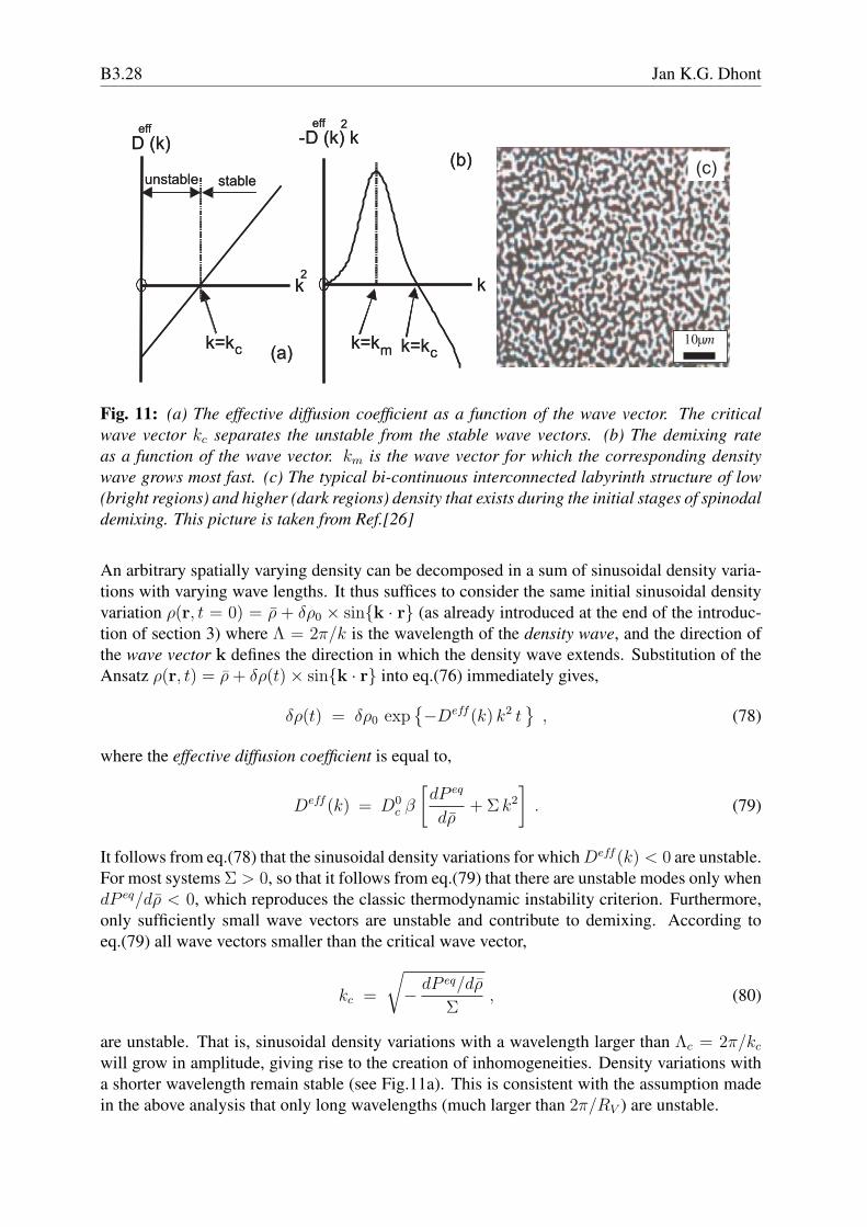
Fig. 11: (a) The effective diffusion coefficient as a function of the wave vector. The criticalwave vector kc separates the unstable from the stable wave vectors. (b) The demixing rateas a function of the wave vector. km is the wave vector for which the corresponding densitywave grows most fast. (c) The typical bi-continuous interconnected labyrinth structure of low(bright regions) and higher (dark regions) density that exists during the initial stages of spinodaldemixing. This picture is taken from Ref.[26]
An arbitrary spatially varying density can be decomposed in a sum of sinusoidal density varia-tions with varying wave lengths. It thus suffices to consider the same initial sinusoidal densityvariation ρ(r, t = 0) = ρ + δρ0 × sin{k · r} (as already introduced at the end of the introduc-tion of section 3) where Λ = 2π/k is the wavelength of the density wave, and the direction ofthe wave vector k defines the direction in which the density wave extends. Substitution of theAnsatz ρ(r, t) = ρ + δρ(t)× sin{k · r} into eq.(76) immediately gives,
δρ(t) = δρ0 exp{−Deff (k) k2 t
}, (78)
where the effective diffusion coefficient is equal to,
Deff (k) = D0c β
[dP eq
dρ+ Σ k2
]. (79)
It follows from eq.(78) that the sinusoidal density variations for which Deff (k) < 0 are unstable.For most systems Σ > 0, so that it follows from eq.(79) that there are unstable modes only whendP eq/dρ < 0, which reproduces the classic thermodynamic instability criterion. Furthermore,only sufficiently small wave vectors are unstable and contribute to demixing. According toeq.(79) all wave vectors smaller than the critical wave vector,
kc =
√− dP eq/dρ
Σ, (80)
are unstable. That is, sinusoidal density variations with a wavelength larger than Λc = 2π/kc
will grow in amplitude, giving rise to the creation of inhomogeneities. Density variations witha shorter wavelength remain stable (see Fig.11a). This is consistent with the assumption madein the above analysis that only long wavelengths (much larger than 2π/RV ) are unstable.
Diffusion B3.29
Note that when the higher order spatial derivatives in the diffusion equation (76) (correspondingto the contribution ∼ Σ in eq.(79) for the effective diffusion coefficient) are omitted for unsta-ble systems, arbitrary short wavelength density variations demix arbitrary fast. This is clearlyunphysical, so that the higher order spatial derivatives are essential for a realistic description ofdemixing, contrary to the diffusion in stable systems.The rate with which density variations grow, according to eq.(78), is equal to−Deff (k) k2. For,
km =
√− dP eq/dρ
2Σ= kc/
√2 , (81)
the growth rate attains a maximum value (see Fig.11b). The amplitude of the density variationwith a wavelength equal to Λm = 2π/km thus grows faster than any other demixing densitywave. This introduces a characteristic length scale of inhomogeneities. Since the growth ratesare independent of the direction of the wave vector, a bi-continuous interconnected labyrinthstructure of low and higher density exists during the initial stages of demixing. A sketch ofsuch a labyrinth structure is given in Fig.11c. The width of the labyrinth substructures are equalto the wavelength Λm of the most fast growing density wave.
4.3 The microscopic origin of the spinodal instabilityTo understand on a microscopic level why a system can become thermodynamically unstable,let us rewrite the generalized diffusion equation (52) as,
∂
∂tδρ(r, t) = −β D0
c ∇ · ρ(r, t)[FBr(r, t) + FInt(r, t)
], (82)
where,
FInt(r, t) = −∫
dr′ g(r, r′, t) ρ(r′, t)∇V (|r− r′ |) , (83)
is the direct force, which stems from inter-molecular potential interactions (as specified by thepair-potential V ) and,
FBr(r, t) = −kBT ∇ ln{ρ(r, t)} , (84)
is the Brownian force on a molecule at the position r. Now consider a molecule at r in aninhomogeneous environment, as sketched in Fig.12a. The inhomogeneous macroscopic densitymay be thought of as an instantaneous realization of the fluctuating density. A little thoughtshows that the Brownian force is always directed towards the region with lower concentration,as depicted in Fig.12a. Now suppose that the pair-interaction potential is purely attractive. Thedirect force FInt is then directed in the opposite direction, towards the region with a larger den-sity, since in that region there are more neighbouring molecules attracting the molecule underconsideration : this can also be seen formally from eq.(83) for the direct force, using a purely at-tractive pair-interaction potential. On lowering the temperature, the Brownian force diminishes,since that force is directly proportional to the temperature. The direct force, however, increasesin magnitude, due to the fact that the pair-correlation function becomes more pronounced (toleading order in the density this follows from the expression g = exp{−V/kBT}, where V < 0for an attractive pair-potential). At the temperature where |FInt |>|FBr |, the net force on themolecule is directed towards the region with a larger density. This is the mechanism that isresponsible for uphill diffusion, and leads to phase separation.
B3.30 Jan K.G. Dhont
(c)“froozen”
scattering
patternr
BrFr
IFr
position
(a)
ik
r
sk
r
detector
sampleincident beam
(b)
Q
scattering
angle
(c)“froozen”
scattering
patternr
BrFr
IFr
position
r
BrFr
IFr
position
(a)
ik
r
sk
r
detector
sampleincident beam
(b)
Q
scattering
angle
ik
r
sk
r
detector
sampleincident beam
(b)
Q
scattering
angle
Fig. 12: (a) The direct and Brownian force on a molecule, indicated by •, in an inhomogeneoussystem. For an attractive direct force FI , its direction is towards the region with larger concen-tration, as sketched here. (b) A schematic of the scattering set up. The wave vector is the equalto ks − ki, with ks the scattered wave vector and ki the incident wave vector, which both havea length equal to 2π/λ, where λ is the wavelength of the light beam. (c) The scattered intensityfrom a suspension of stearyl-coated silica particles as a function of the scattering angle. Eachcurve is measured 10 seconds after each other. At later times, the scattering peak ”freezes”,due to the formation of a gel in the regions of higher concentration. From Ref.[27].
4.4 A light scattering experimentThe above predictions can be verified by means of time resolved light scattering. It can beshown that the time-dependent scattered intensity I(t) at very small scattering angles from aninhomogeneous system is given by (see, for example, Ref.[12]),
I(k, t) ∼ <|δρ(k, t) | 2> , (85)
where the brackets < · · · > refer to ensemble averaging over initial conditions. The wave vectorcan be varied through variation of the scattering angle Θ (the angle between the incident beamand the direction of detection: see Fig.12b)). In case of scattering, the wave vector is equal tok = ks − ki, where ki and ks point in the direction of the incident beam and the direction ofdetection, respectively. In case of elastic scattering, both the incident and scattered wave vectorks and ki have the same length equal to 2π/λ, where λ is the wavelength of the light. It followsthat k = 4π
λsin{Θ/2} ≈ 2π
λΘ, for small scattering angles Θ. The wave vector thus determines
the position on a screen at which scattered light is collected, as sketched in Fig.12b. Substitutionof eq.(78) into eq.(85) gives,
I(k, t) ∼ < δρ20 > exp
{−2 Deff (k) k2 t}
. (86)
This result predicts that in the initial stage of decomposition, ln{I(k, t)} is a linear function intime and that the intensity develops a ”ring-like scattering pattern”, where the position of thepeak grows at a time-independent position. This is indeed observed in some systems, like indispersions of stearyl silica colloidal particles [27]. As can be seen from the plots in Fig.12c, thering-like scattering pattern for this particular system ”freezes” at some time during demixing.This is due to the formation of a gel-like phase in the more concentrated region of the labyrinthstructure. In other systems (see, for example, Refs.[28, 29]), the peak position of the scattering
Diffusion B3.31
ring is observed to shift to lower scattering angles right from the start of the experiment. Sucha shift of position of the peak of the ring-like scattering pattern is expected in the intermediatestage of demixing (the above analysis has been extended to include the intermediate stage inRefs.[12, 30]). Probably the time range within which the linear theory applies is already past atthe time a first reliable measurement could be performed.Spinodal decomposition is also found for hydrogen dissolved in palladium, within the two-phase region in Fig.8a. The required attractive interactions between the H-atoms is probablydue to palladium-crystal-environment mediated interactions.
References[1] R. Festa, E. Galleani d’Agliano, Physica A 90, 229 (1978)
[2] L. Gunther, M. Revzen, A. Ron, Physica A 95, 367 (1979)
[3] M.P. Lettinga, E. Grelet, Phys. Rev. Lett. 99, 197802 (2007)
[4] E. Pouget, E. Grelet. M.P. Lettinga, Phys. Rev. E 84, 041704 (2011)
[5] C. Dalle-Ferrier, M. Kruger, R.D.L. Hanes, S. Walta, M.C. Jenkins, S.U. Egelhaaf, SoftMatter 7, 2064 (2011)
[6] K. Kang, J.K.G. Dhont, J. Chem. Phys. 122, 044905 (2005)
[7] K. Kang, J.K.G. Dhont, J. Chem. Phys. 124, 044907 (2006)
[8] K. Kang, J.K.G. Dhont, J. Chem. Phys. 126, 214501 (2007)
[9] P.-G. de Gennes, J. Chem. Phys. 55, 572 (1971)