Diffusion Through a Half Space: Equivalence Between ... · PDF fileDiffusion Through a Half...

Applied Mathematical Sciences, Vol. 8, 2014, no. 155, 7727 - 7748

HIKARI Ltd, www.m-hikari.com http://dx.doi.org/10.12988/ams.2014.49723

Diffusion Through a Half Space:

Equivalence Between Different Formulations of

the Unique Solution

Michele Mantegna and Luigi Pietro Maria Colombo

Politecnico di Milano, Department of Energy

Via Lambruschini, 4 – 20156 Milano (Italy)

Copyright © 2014 Michele Mantegna and Luigi Pietro Maria Colombo. This is an open access

article distributed under the Creative Commons Attribution License, which permits unrestricted

use, distribution, and reproduction in any medium, provided the original work is properly cited.

Abstract

Diffusion through a half space involves a classical parabolic partial differential

equation that is encountered in many fields of physics and has significant

engineering applications, concerning particularly heat and mass transfer. However,

in the specialized literature, the solution is usually achieved restricting the

problem to particular cases and attaining apparently different formulations, thus a

comprehensive overview is hindered. In this paper, the solution of the diffusion

equation in a half space with a boundary condition of the first kind is worked out

by means of the Fourier’s Transform, the Green’s function and the similarity

variable, with a proof of equivalence – not found elsewhere – of these different

approaches. The keystone of the proof rests on the square completion method

applied to Gaussian-like integrals, widely used in Quantum Field Theory.

Keywords: Parabolic PDE, Dirichelet problem, Mass diffusion, Heat Conduction,

Square Completion Method

1 Introduction

One of the most important mathematical methods of Quantum Field Theory is

square completion to compute Gaussian integrals that arise from the Path Integral

7728 Michele Mantegna and Luigi Pietro Maria Colombo

Approach pioneered by Feynman [1 - 2]. As Zee [3] says, “Believe it or not, a

significant fraction of the theoretical physics literature consists of performing

variations and elaborations of this basic Gaussian integral”. Although all books at

the advanced undergraduate and most books at the graduate level use the method

of canonical quantization (which avoids Gaussian integrals) or defer path integrals

to the last chapters, the book by Zee introduces path integrals from the beginning.

The purpose of this paper is to show how the square completion method to

compute Gaussian-like integrals allows understanding the equivalence of

apparently very different formulations of the solution of the standard parabolic

PDE encountered in heat conduction and other diffusion problems that play an

important role in many Engineering applications. A paper by Slutsky [4] applied

the full-blown machinery of path integrals to diffusion in the context of polymer

physics. A similar though shorter treatment of linear polymer molecules as

random walks is found in earlier works such as the books by Schulman [5] and

Carrà [6]. On the other hand, Hall [7] very recently discussed the connection

between random walks and path integrals. Our purpose is somewhat more limited

and, at the same time, more accessible to a broader audience. We want to show

that an important integral, which lies at the core of the path integral approach to

Quantum Field Theory, emerges naturally from the juxtaposition of classical

methods to solve the diffusion PDE and highlights the hidden connections among

them.

2 Problem Statement

We consider an important class of partial differential equations in the general

form

uDt

u 2

(1)

belonging to the category of parabolic equations. They are used to represent in

different contexts a kind of transport referred to as diffusion [8]. For instance,

setting

Tu , temperature [K] and D , thermal diffusivity [m2 s-1], Eq. (1)

describes heat conduction in a homogeneous isotropic continuum with

constant properties and without heat sources. This equation was first derived

by Fourier [9].

Acu , molar concentration of the chemical species A [mol m-3] and

ABDD , binary diffusivity [m2 s-1], Eq. (1) describes ordinary diffusion of

the chemical species A in a binary mixture A+B with constant total

concentration BA ccc . This equation was first derived by Fick. A more

general form would involve the chemical potential of the species [10] but this

approximation still describes a wide field of applications. For example, a

Diffusion through a half space 7729

classical problem in Metallurgy is the estimate of the decarburization depth in

steel [11]. A variant of the diffusion PDE is also used in Nuclear Reactor

Physics to model neutron density in the one-speed approximation [12].

u , probability density function of the velocity of a particle and D ,

diffusion coefficient. This is known as the Fokker-Planck equation with zero

drift coefficient [13]. It is interesting to note that this equation has been

recently applied beyond Physics to study the volatility in financial markets

[14].

A classical problem is the determination of txuu , in a half space 0x ,

initially at a uniform value 0u with the interface subjected to a first kind

boundary condition for 0t (Dirichelet’s problem). The differential problem is

stated as

02

2

0 ttxx

uD

t

u

(2a)

00 0 ttxuu (2b)

00 ttxtuu i (2c)

00 ttxuu (2d)

It is convenient to set 00 u (note that if u is a solution, 0uu is a solution

as well) and 00 t conventionally.

3 General Solution by Means of Fourier Analysis

The problem is approached by the Fourier analysis [15]. At first, we consider

the Fourier transform of Eq. (2c) with respect to time

dttitxuxU

exp,02

1,0 (3)

where is the angular frequency [rad s-1]. On the other hand, txu ,0 is

recovered by the antitransform

dtixUtxu exp,02

1,0 (4)

Notice that Eqs. (3) and (4) have the same coefficient 212

. However,

different choices are possible. The reader is referred to Appendix A for a brief

discussion on this subject.

The variable separation method is applied to Eq. (2a) looking for particular

solutions in the form


tixXtxu e x p, (5)

as suggested by the integrand in Eq. (4).

Replacing in Eq. (2a) and dividing both members by tiexp , an ordinary

differential equation is obtained:

02

2

XD

i

dx

Xd (6)

The characteristic equation associated to Eq. (6) is

02 D

i (7)

giving

D

i (8)

which is often called wavenumber [16] [rad m-1].

Hence, the general solution of Eq. (6) turns out to be

x

D

iCx

D

iCxX

e x pe x p (9)

Replacing in Eq. (5)

x

D

itiCx

D

itiCtxu

e x pe x p;, (10)

which is often called a thermal wave even though the second-order derivative with

respect to time, characteristic of the wave equation, does not appear in Eq. (1). A

thorough discussion about the concept of wave and thermal waves is given by

Salazar [17].

The boundary conditions Eqs. (2c) and (2d) are applied to calculate the

coefficients C and C .

From Eq. (2c)

tixUtiCCtxu e x p0,e x p;,0 (11)

then

,0 xUCC (12)

From Eq. (2d)

0;,lim

txux

(13)


Eq. (13) is applied under the assumption that D is real and positive. This

requirement is actually a consequence of the second principle of thermodynamics.

On the other hand, if D were imaginary Eq. (1) would turn into the well-known

Schrödinger equation which does not describe diffusive transport, hence is not

treated here.

If 0 , recalling that

D

iD

i

21

(14)

Eq. (10) becomes

xD

xD

tiC

xD

xD

tiCtxu

2e x p

2e x p

2exp

2exp;,

(15)

Passing to the limit, Eq. (13), as u must be finite 0 C is obtained.

Hence

x

DitixUtxu

21e x p0,00;,

(16)

Repeating the same procedure for 0

x

DitixUtxu

21e x p0,00;,

(17)

If 0 , Eq. (15) reduces to a constant that can be neglected as Eq. (2a)

only contains derivatives of u.

A unique representation is obtained introducing the sign function, strictly

related to the Heaviside step function as it will be shown in Section 5:

xD

itixUtxu2

s g n1e x p,0;,

(18)

By integration over the angular frequency it is obtained

dxD

itixUtxu2

s g n1e x p,02

1, (19)

which, for 0x , reduces to Eq. (4).

Finally, to eliminate the transformed function U it is convenient to express

the boundary condition Eq. (2c) from Eq. (3) as follows


dtdxD

ittitxutxut

2sgn1exp,0

2

1,

(20)

Handbooks usually report particular cases of Eq. (20). The reader should address

in particular the book of Prestini [18] where the presented approach is developed

in a less general way but with very interesting practical applications. Restricting

the attention to the heat conduction problem, many authors deal with the cases of

constant and periodic heating [19 - 26] though the general problem is not

discussed in detail.

4 The Similarity Solution

Most of the cited bibliography directly refer to the similarity solution of (2a).

Actually, dimensional analysis shows that the dependence on x and t is

condensed in the combinations

BDt

x

Dt

xB or

2

(21)

The former is sometimes called the Boltzmann number, whereas the latter is

simply known as the similarity variable. The physical meaning of B is discussed

in Appendix B.

Generally speaking, similarity solutions are only a subset of the existing

solutions. In this case, however, it can be shown that all the solutions are

self-similar.

Adopting the Boltzmann number, the following identities hold

x

B

x

B

t

B

t

B 2 and

(22)

dB

du

t

B

t

u

(23)

dB

du

x

B

x

u 2

(24)

2

2

2

2

22

2 42

dB

ud

x

B

dB

du

x

B

x

u

(25)

Hence, replacing in Eq. (2a), an ordinary differential equation is obtained:


04

22

2

dB

du

B

B

dB

ud (26)

which is written as a first order equation setting dBduu

04

2

u

B

B

dB

ud

(27)

Integration yields

4e x p

1

BB

Cu (28)

Restoring dBduu and performing a second integration taking into account

Eq. (21)

2

2

14

e x p2 CdCu

(29)

The integral in Eq. (29) cannot be evaluated as a combination of elementary

functions. It is a transcendental function as it is shown by the Liouville’s theory

[27].

It is customary to define the error function

z

dxxzerf

0

2exp2

(30)

such that

1lim and 00z

zerferf (31)

It is then obtained from Eq. (29)

21

2e r f CCu

(32)

where multiplicative factors and additive constants have been lumped in 1C and

2C respectively.

A particularly useful case study is obtained if Eq. (2c) is written as

1 ,0 ,0 uxt . This implies 12 C whereas the initial condition Eq. (2b)

yields 11 C so that

2e r f1

u (33)

This is the response of the half-space to a step variation of u on its interface.

Figures 1a and 1b report 2u and txu , , respectively, to clarify the meaning

of the term similarity. It is evident that each spatial distribution of u at a certain

time instant is self-similar because, when reported in terms of the similarity

variable , all the distributions collapse into a unique curve.


(a)

(b)

Figure 1 – Response of the half-space to a step variation of u on its interface in

terms of the similarity variable (a) and of the natural variables (b).

It is also evident that the diffusive transport described by (1) occurs

instantaneously in contrast with the basic tenets of Special Relativity. Actually,

since txu , 0 , the propagation speed turns out to be infinite, meaning that

the effect of a perturbation at the interface 0x is immediately felt at any

distance from the interface. This is a theoretical problem arising from the

constitutive equations relating the diffusive flux to the gradient of u , such as

Fourier’s law and Fick’s first law. However, this effect is quite small in the most

common situations and it is usually neglected [28].

To show that all the solutions of the problem defined by Eqs. (2a) to (2d) are

self-similar, it is convenient to switch to a dimensionless formulation. Recalling

the definition of the Boltzmann number, Eq. (21), characteristic time ct and

length cL are chosen arbitrarily such that

12

c

c

Dt

L (34)

As 0ct , cc DtL and, choosing cu as a characteristic value of u, the

following set of dimensionless quantities is identified


ccc u

uu

t

tt

L

xx , , (35)

Replacing in Eqs. (2a) to (2d) the dimensionless problem results

00 2

2

txx

u

t

u (36a)

00 1 txu (36b)

00 txtuu i (36c)

0 1 txu (36d)

Hence, iutxuu ;, or ciccc uuttDtxuuu ;, , the latter

showing that a double infinity of solutions is derived by choosing arbitrarily cu

and ct , i.e. the set of all the solutions is split into two equivalence classes. As

each class includes only self-similar solutions, all the possible solutions are

self-similar.

At this point it is interesting to seek a general solution of problem defined by

Eqs. (2a) to (2d) in the form of infinite series of particular solutions like Eq. (33)

where self-similarity is evident rather than Eq. (20). In the following it is

discussed the method for representing the new form of the solution and the

equivalence with Eq. (20).

5 Integral Representations of the Dirac’s Function and

Heaviside’s Step Applied to the Diffusion Problem

The Dirac’s delta function is defined as [29]

1

0

,0

dxx

Rxx

(37)

Accordingly, an important property is that any function yf can be

represented as

dxxyxfyf (38)

There are different representations [30] of such a function that today

mathematicians prefer to call more properly a distribution. A useful one for the


purpose of this paper is found in Mandl [31]

dyixyx exp2

1

(39)

The following developments justify this choice. Actually, if Eq. (3) is replaced

in Eq. (4), it yields

dtdttitxutxut

exp,2

1, (40)

On the other hand, according to Eq. (38)

t

tdtttxutxu ,, (41)

Comparing Eq. (40) and Eq. (41) it is seen that

dttitt exp2

1 (42)

which is equivalent to Eq. (39).

The Heaviside’s step function is defined as [3]

10 ,210 ,00 tHtHtH (43)

The relation between H and the sign function used in Eq. (20) is formally

expressed as

12s g n tHt (44)

The application of the step function usually requires, as seen for the Dirac’s

delta, suitable representations. For the purpose of this paper, it is convenient to

use the following [32]:

dzz

itz

itH

exp

2

1

(45)

Considering Eq. (39) it can be shown that

tdt

tdH (46)

which is more easily understood if H is thought as the limit of a ramp that rises

from 0 to 1 about 0t .

This relation is useful to transform Eq. (38) in another useful representation of

any continuous function. Integrating by parts


tdtd

dfttHf

tdtd

dfttHttHtf

tdttd

ttdHtftdtttftf

(47)

The geometrical meaning of Eq. (47) is a representation of tf as the

superposition of elementary steps of height df (Duhamel’s formula) [20].

Equation (47) is then applied to the solution of problem defined by Eqs. (2a) to

(2d) as follows:

td

t

tuttHutxu

,0,0,0 (48)

where 0,0 u since no perturbation is applied at the interface before the

initial time. In any case, the value of ,0u would be only an additive constant.

The same holds for ,0u since any physical perturbation has finite duration.

The solution is then built as a continuous linear combination of the particular

solution, Eq. (33), corresponding to the response of the half space to a constant

perturbation at the interface, that is

td

ttD

xe r f

t

tuttHtxu

21

,0, (49)

It is worthwhile noting that the argument of the error function is prevented

from assuming imaginary values when tt because, in this case, 0 ttH .

Equation (49) clearly shows that the diffusion process obeys to the principle of

delayed causality. Actually, a generic boundary condition at the interface is

decomposed as the superposition of elementary steps, the response to which is

delayed by the time interval tt . Some attempts to modify the Fourier’s law in

order to prevent an infinite speed of propagation of the perturbations, as observed

in the previous section, happened to violate the delayed causality principle [33].

6 Solution by Means of the Green’s Function

The solution of Eq. (2a) in the same form as Eq. (20) is also obtained by

means of the Green’s function [34]. Since the derivation is less straightforward

than making use of the Fourier’s transform, only an outline will be given in the

following. For this purpose, it is convenient to consider the inhomogeneous

diffusion equation:


txSx

uD

t

u,

2

2

(50)

where xtS , physically represents a source term.

The Green’s function xtG , is the solution of Eq. (50) if

txtxtxS ,, 2 (51)

under appropriate initial and boundary conditions, that is

txx

GD

t

G,2

2

2

(52)

The relation between u and G is found as

t x

tdxdttxxGtxStxu ,,, (53)

The Green’s function is determined as follows.

At first, txG , is written as Fourier’s back-transform of ,g :

ddxtigtxG exp,2

1,

2

(54)

Then the partial derivatives that appear in Eq. (52) result respectively

ddxtigit

Gexp,

2

12

(55)

ddxtigx

Gexp,

2

1 2

22

2

(56)

Furthermore, from Eq. (39) it is found

ddxtitx exp2

1,

2

2 (57)

Replacing Eqs. (55), (56) and (57) in Eq. (52) the Fourier’s back-transform of

the Green’s function results

2

1,

Dig

(58)


Hence, from Eq. (54)

ddDi

xtitxG

22

exp

2

1, (59)

which is more conveniently rewritten as

dxItitxG

,exp2

1,

2 (60)

with

d

Di

xixI

2

exp, (61)

Integration is performed by means of the residuals theorem and the Jordan’s

lemma in the complex plane along the loop depicted in Figure 2. The integration

loop is suitably selected so that, when lR , only the contribution along the

diameter (which extends to the whole real axis) is different from zero, as a

consequence of the Jordan’s lemma.

The integrand poles are:

DiP

DiP

210

210

(62)

Figure 2 – Integration loop and poles of the integrand for Eq. (61). Black dots

represent the poles for 0 , the white ones for 0 .


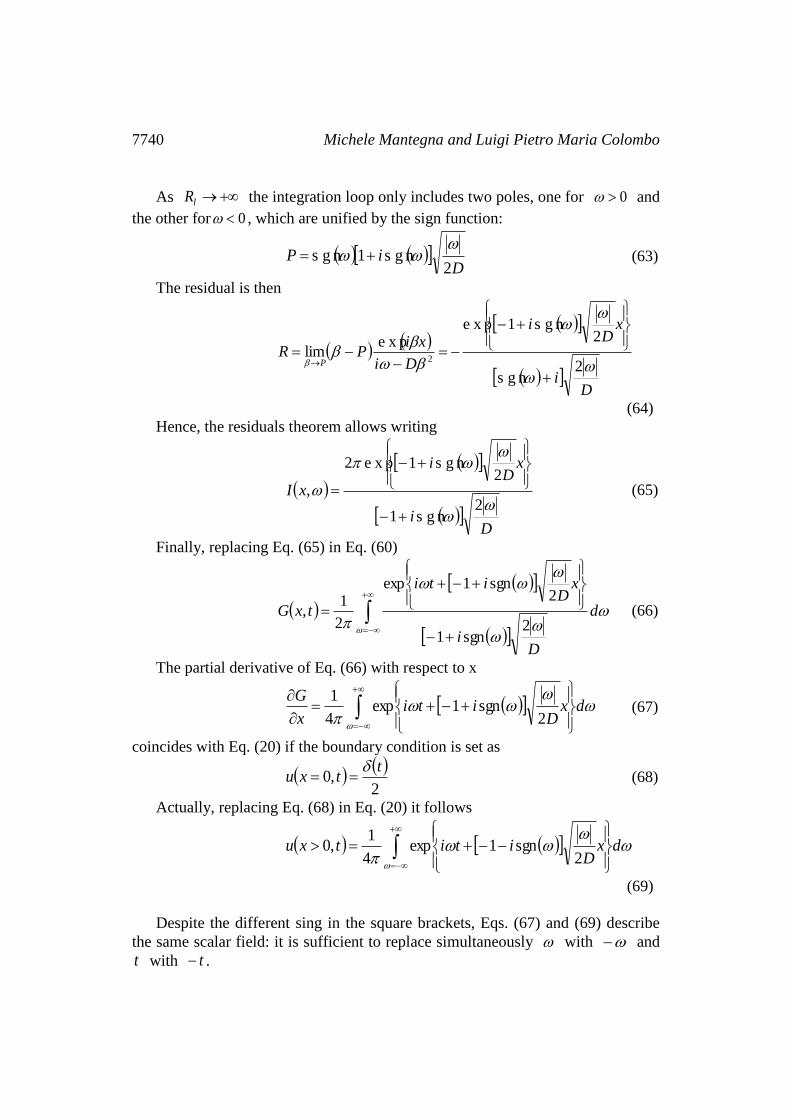
As lR the integration loop only includes two poles, one for 0 and

the other for 0 , which are unified by the sign function:

D

iP2

s g n1s g n

(63)

The residual is then

D

i

xD

i

Di

xiPR

P

2s g n

2s g n1e x p

e x plim

2

(64)

Hence, the residuals theorem allows writing

D

i

xD

i

xI

2

s g n1

2s g n1e x p2

,

(65)

Finally, replacing Eq. (65) in Eq. (60)

d

Di

xD

iti

txG2

sgn1

2sgn1exp

2

1, (66)

The partial derivative of Eq. (66) with respect to x

dxD

itix

G

2sgn1exp

4

1 (67)

coincides with Eq. (20) if the boundary condition is set as

2

,0t

txu

(68)

Actually, replacing Eq. (68) in Eq. (20) it follows

dxD

ititxu2

sgn1exp4

1,0

(69)

Despite the different sing in the square brackets, Eqs. (67) and (69) describe

the same scalar field: it is sufficient to replace simultaneously with and

t with t .


In summary, it has been shown that the solution of Eq. (2a) with the boundary

condition Eq. (68) is equivalent to the solution of Eq. (52). In other words,

through the Green’s function the solution of the homogeneous diffusion equation

is derived from the inhomogeneous one endowed with a suitable source term.

7 Equivalence of the General Solutions by Means of the Square

Completion Method

Apparently, the two general solutions developed in Sections 3 and 5,

respectively, are quite different. In particular, Eq. (20) involves two improper

integrals whereas only one appears in Eq. (49); Eq. (20) involves complex

functions, whereas Eq. (49) is restricted to the real field; Eq. (20) involves the

boundary condition tu ,0 , whereas its derivative with respect to time appears in

Eq. (49). Nevertheless, the boundary value problems involving Eq. (1) do have a

unique solution [19] so that Eq. (20) and Eq. (49) must be equivalent. The proof

of equivalence is given in the following.

Equation (20) is written as

dxD

itdttitxutxu

t2

sgn1expexp,02

1,

(70)

The inner integral is solved by parts considering that

0,0,0 txutxu

tdtti

t

txu

itdttitxu

t

exp,01

exp,0 (71)

Replacing in Eq. (70)

t

tdt

txudx

Di

tti

itxu

,0

2sgn1exp

exp

2

1,

(72)

Comparison between Eq. (49) and Eq. (72) shows that their equivalence

would imply

dx

Di

tti

i

ttD

xerfttH

2sgn1exp

exp

2

1

21

(73)


Denoting the left hand side as 1M and the right hand side as 2M , both are

rewritten eliminating H and sgn

ttDx

dM2

2

1 exp2

(74)

dxD

itti

iM exp

1

2

12 (75)

It will be shown that

x

M

x

M

21 (76)

which implies 21 MM apart from an integration constant that is equal to zero

according to the initial condition Eq. (2b).

From the Leibnitz formula

ttD

x

ttDx

M

4e x p

1 2

1

(77)

dx

D

itti

D

i

ix

Mexp

2

12 (78)

The latter expression is manipulated as first by applying to the argument of the

exponential the square completion method [35], widely used in Quantum Field

Theory to compute path integrals [5], [36].

ttD

x

ttD

xttix

D

itti

42

22

(79)

Hence

d

ttD

xtti

D

i

ttD

x

ix

M2

2

2

2e x p

4e x p

2

1

(80)

The integral in Eq. (80) is solved by substitution setting

ttD

xttiy

2 (81)


Hence

dyy

ttDd

ttD

xtti

D

i 2

2

exp2

2exp

(82)

Further replacing 2

22 z

y implying dzi

dy2

2

dz

z

idyy

2exp

2

2exp

22 (83)

It is known [36] that

22

e x p2

dzz

(84)

Incidentally, it is worthwhile mentioning that the first mathematician who

studied the so-called Gaussian integrals was not Gauss but De Moivre in 1733

[37].

Replacing Eqs. (62) to (64) in Eq. (80) yields, finally

x

M

ttD

x

ttDx

M

1

2

2

4e x p

1

(85)

The equivalence of Eq. (20) and Eq. (49) is then proven thanks to the decisive

resort to the square completion method, just as in many gaussian-like integrals

found in the path integral approach to Quantum Field Theory.

Appendix A

A few not quite trivial aspects about the Fourier transform require explanation

to avoid misunderstanding. Eqs. (3) and (4) represent, respectively, the Fourier

transform and the inverse Fourier transform of a function tu . However, this

representation is not unique, as different choices of the coefficients are possible

[18] provided that their product is 12

. In this paper the symmetric

representation is used, i.e., both the coefficients are set equal to 212

, but it is

also common to find the anti-symmetric convention, where the factor 12

only appears in the inverse Fourier transform. On the other hand, this requirement

on the coefficients could even be removed, as shown in James [38]. The preface

of this book introduces the subject of Fourier’s analysis with this witty remark:

“Showing a Fourier transform to a physics student generally produces the same

reaction as showing a crucifix to Count Dracula”. An interesting historical

overview of the Fourier Transform is given by Bracewell [39].


Appendix B

Dimensional analysis is probably the easiest way to define the Boltzmann

number. Nevertheless, its physical meaning is better understood considering

diffusion at a molecular scale and introducing the concept of random walk [40].

Consider a particle of a species A that diffuses through a substance B

undergoing a random walk described by a broken line ...3210 PPPP where points 0P ,

1P , 2P , ...3P correspond to the particle random strikes. Neither the location of

the points nor the length of the vector paths ... , , 322110 PPPPPP can be predicted.

However, if the random walk is made of a very large number of paths, some

general property is statistically inferred. The final position NP is related to the

starting point 0P by the relation

N

n

nnN PPPP1

10 (B1)

The absolute value of the overall path length is given by

NNN PPPPPP 00

2

0 (B2)

The scalar product in Eq. (B2) is a summation of 2N terms that comprises

two subsets. The first one if formed by N terms referring to the scalar product

of a vector by itself. If N the average value

2

1

2

1

1LPP

N

N

n

nn

(B3)

is interpreted as the square of a random walk characteristic length. Similarly, it is

defined an average time interval t between two successive strikes such that the

final position NP is reached after the time

tNNT (B4)

The second subset contains the remaining NN 2 terms that are scalar

products of couples of vectors nn PP 1

with different indices. Due to the random

nature of the particle motion, these vectors are uncorrelated both in direction and

in absolute value, thus for N their contribution is negligible.

Consequently, from Eqs. (B3) and (B4), Eq. (B2) becomes

t

LTNLPP N

2

22

0 (B5)


This result is written in a more interesting form as

12

2

0

t

LT

PP N

(B6)

where the left hand term shows the same form of the Boltzmann number Eq. (21)

through the correspondences between 2

0 NPP and 2x , T and t , t

L

2

and D .

This heuristic argument is also useful to understand the microscopic origin of

irreversibility: at each interaction of the particle, any information about the

previous one is lost, hence diffusion cannot be inverted. A recent paper by Brazzle

[41] discusses a pedagogical method to simulate diffusion by means of

spreadsheet computation, which is widely available. Actual random walks are

built on a variety of lattices. However the easiest method remains the one

followed by Gautreau [40].

References

[1] R.P. Feynman, A. R. Hibbs, Quantum Mechanics and Path Integrals,

Emended Edition by F. D. Styer, Dover Publications Inc., New York, 2010, p.

58 and p. 359.

[2] B. A. Baaquie, Path Integrals and Hamiltonians: Principles and Methods,

Cambridge University Press, Cambridge, 2014, p. 130.

[3] A. Zee, Quantum Field Theory in a Nutshell, Princeton University Press,

Princeton, 2010, p. 23.

[4] M. Slutsky, Diffusion in a half - space: From Lord Kelvin to path integrals,

Am. J. Phys. 73(4) (2005), 308 - 314.

[5] L. S. Schulman, Techniques and Applications of Path Integration, John

Wiley & Sons, New York, 2005, p. 332.

[6] S. Carrà, Struttura e stabilità: introduzione alla Termodinamica dei materiali,

Mondadori, Milano, 1978, p. 214 (in Italian).

[7] B. C. Hall, Quantum Theory for Mathematicians, Springer - Verlag, New

York, 2013, ch. 20.


[8] S. J. Farlow, Partial Differential Equations for Scientists and Engineers,

Dover Publications, New York, 1993, p. 11.

[9] J. B. J. Fourier, Théorie Analytique de la Chaleur, Firmin Didot & Garçons,

Paris, 1822, reprinted from the original by Editions Jacques Gabay, Scéaux

(1988); the English translation, entitled “The Analytical Theory of Heat”,

first appeared in 1878, has been reprinted in 2009 by Cambridge University

Press.

[10] D. Kondepudi, Prigogine I, Modern Thermodynamics: From Heat Engines to

Dissipative Structures, John Wiley and Sons, West Sussex, 1988, p. 270.

[11] B. Liščić, Steel Heat Treatment in Steel Heat Treatment Metallurgy and

Technologies edited by G.E. Totten, CRC Press, Boca Raton, 2006, ch 6.

[12] M. S. Weston, Nuclear Reactor Physics, Wiley - VCH, Weinheim, 2007, p.

43.

[13] L. D. Landau, E.M. Lifsits, Course of Theoretical Physics: Volume 10,

Pergamon Press, Oxford, 1981, p. 89.

[14] E. Haven, A. Khrennikov, Quantum Social Science, Cambridge University

Press, Cambridge, 2013, p. 40.

[15] M. R. Spiegel, Fourier Analysis with Applications to Boundary Value

Problems, McGraw - Hill, New York, 1974, p. 81.

[16] H. J. Pain, The Physics of Vibrations and Waves, 5th Edition, John Wiley and

Sons, West Sussex, 2005, p. 120.

[17] A. Salazar, Energy Propagation of Thermal Waves, Eur. J. Phys., 27 (2006),

1349 - 1355.

[18] E. Prestini, The Evolution of Applied Harmonic Analysis: Models of the Real

World, Birkhauser, Boston, 2004.

[19] H. S. Carslaw, J.C Jaeger., Conduction of Heat in Solids, Clarendon Press,

Oxford, 1959, p. 51.

[20] M. N. Ozisik, D.W. Hahn, Heat Conduction, 3rd Edition, John Wiley and

Sons, New Jersey, 2012, p. 236.

[21] L. M. Jiji, Heat Conduction, Jaico Pubishing House, Mumbai, 2003, p. 104.


[22] M. Moares, Time Varying Heat Conduction in Solids, in Heat Condution:

Basic Research, edited by V. S. Vikhrenko, InTech, Croazia, 2011.

[23] W. M. Rohsenow, J. R. Hartnett, Y.I. Cho, Handbook of Heat Transfer,

McGraw - Hill, New York, 1998.

[24] F. Kreith, R. M. Manglik, M.S. Bohn, Principles of Heat Transfer, 7th

Edition, Cengage Learning, Australia, 2011.

[25] T. L. Bergmann, A. S. Lavine, F.P. Incropera, D. P. Dewitt, Introduction to

Heat Transfer, 7th Edition, John Wiley and Sons, West Sussex, 2011, p. 327.

[26] A. Bejan, Heat Transfer, John Wiley and Sons, 1993, p.148.

[27] J. F. Ritt, Integration in Finite Terms: Liouville’s Theory of Elementary

Methods, Columbia University Press, New York, 1948, p. 49.

[28] A. N. Smith, P.M. Norris, Microscale Heat Transfer, in Heat Transfer

Handbook, edited by A. Bejan and A. D. Kraus, John Wiley and Sons,

Hoboken, 2003, p. 1331.

[29] P. A. M. Dirac, The Principles of Quantum Mechanics, 4th Edition, Oxford

University Press, Oxford, 1968.

[30] B. R. Kusse, Mathematical Physics: Applied Mathematics for Scientists and

Engineers, Wiley-VCH, 2006, ch. 5.

[31] F. Mandl, Quantum Mechanics, in The Manchester Physics Series, John

Wiley and Sons, West Sussex, 1997.

[32] V. I. Smirnov, A Course of Higher Mathematics: Advanced calculus,

Pergamon Press, Oxford, 1964.

[33] M. Ferenc, Can a Lorentz Invariant Equation Describe Thermal Energy

Propagation Problems?, in Heat Condution: Basic Research, edited by V. S.

Vikhrenko, InTech, Croazia, 2011.

[34] L. D. Landau and E. M. Lifshits, Course of Theoretical Physics: Volume 9,

Pergamon Press, Oxford, 1981, p. 28.

[35] J. E. Kaufmann, K. L. Schwitters, Elementary Algebra, 8th Edition,

Thomson Brooks/Cole, Canada, 2007, p. 433.


[36] S. Weinberg, The Quantum Theory of Fields, Cambridge University Press,

Cambridge, 1995, vol. 1, p. 421.

[37] U. C. Merzbach and C. B. Boyer, A History of Mathematics, 3rd edition,

John Wiley and Sons, New Jersey, 2011, p. 374.

[38] J. F. James, A Student’s Guide to Fourier Transforms With Applications in

Physics and Engineering, Cambridge University Press, Cambridge, 2002, p.

9.

[39] R. N. Bracewell, The Fourier’s Transform, Sci. Am., 6 (1989), 62.

[40] R. Gautreau, W. Savin, Modern Physics, 2nd Edition, McGraw-Hill, New

York, 1999, p. 263.

[41] B. Brazzle, A Random Walk to Stochastic Diffusion through Spreadsheet

Analysis, Am. J. Phys., 81(11) (2013), 823 - 828.

Received: September 11, 2014; Published: November 3, 2014

Date post:	07-Feb-2018
Category:	Documents
Upload:	dangxuyen
View:	216 times
Download:	0 times

Diffusion Through a Half Space: Equivalence Between ... · PDF fileDiffusion Through a Half...

Documents