Diffusive Transport Approach

8/3/2019 Diffusive Transport Approach

http://slidepdf.com/reader/full/diffusive-transport-approach 1/16

A diffusive transport approach for flow routing

in GIS-based flood modeling

Y.B. Liua,*, S. Gebremeskela, F. De Smedta, L. Hoffmannb, L. Pfisterb

a Department of Hydrology and Hydraulic Engineering, Vrije Universieit Brussel, Pleinlaan 2, 1050 Brussels, Belgiumb Research Unit in Environment and Biotechnologies, Centre de Recherche Public-Gabriel Lippmann, Grand-Duchy, Luxembourg

Received 11 October 2002; accepted 23 June 2003

Abstract

This paper proposes a GIS-based diffusive transport approach for the determination of rainfall runoff response and flood

routing through a catchment. The watershed is represented as a grid cell mesh, and routing of runoff from each cell to the basin

outlet is accomplished using the first passage time response function based on the mean and variance of the flow timedistribution, which is derived from the advection–dispersion transport equation. The flow velocity is location dependent and

calculated in each cell by the Manning equation based on the local slope, roughness coefficient and hydraulic radius. The

hydraulic radius is determined according to the geophysical properties of the catchment and the flood frequency. The total direct

runoff at the basin outlet is obtained by superimposing all contributions from every grid cell. The model is tested on the Attert

catchment in Luxembourg with 30 months of observed hourly rainfall and discharge data, and the results are in excellent

agreement with the measured hydrograph at the basin outlet. A sensitivity analysis shows that the parameter of flood frequency

and the channel roughness coefficient have a large influence on the outflow hydrograph and the calculated watershed unit

hydrograph, while the threshold of minimum slope and the threshold of drainage area in delineating channel networks have a

marginal effect. Since the method accounts for spatially distributed hydrologic and geophysical characteristics of the

catchment, it has great potential for studying the influence of changes in land use or soil cover on the hydrologic behavior of a

river basin.

q 2003 Elsevier B.V. All rights reserved.

Keywords: Diffusive wave; Unit hydrograph; First passage time distribution; Geographical information system; Flood modeling

1. Introduction

In flood prediction and rainfall– runoff compu-

tation, physically based distributed modeling of

watershed processes has become increasingly feasible

in recent years. In addition to the development of

improved computational capabilities, Digital

Elevation Model (DEM), digital data of soil type

and land use, as well as the tools of Geographical

Information System (GIS), give new possibilities for

hydrologic research in the understanding of the

fundamental physical processes underlying the hydro-

logic cycle and of the solution of the mathematical

equations representing those processes.

0022-1694/$ - see front matter q 2003 Elsevier B.V. All rights reserved.

doi:10.1016/S0022-1694(03)00242-7

Journal of Hydrology 283 (2003) 91–106

www.elsevier.com/locate/jhydrol

* Corresponding author. Tel.: þ32-2-629-3335; fax: þ32-2-629-

3022.

E-mail addresses: [email protected] (Y.B. Liu), fdesmedt@

vub.ac.be (F. De Smedt).

http://www.elsevier.com/locate/jhydrol

http://www.elsevier.com/locate/jhydrol



Flood prediction and catchment modeling are main

topics facing the hydrologist dealing with processes of

transforming rainfall into a flood hydrograph and the

translation of hydrographs throughout a watershed.

The theory of the unit hydrograph for the prediction of

stream flow in a basin has played a prominent role in

hydrology for several decades since its development.

This system response theory assumes that the basin

response to a rainfall input is linear and time invariant.

The discharge at the outlet of the basin is given by theconvolution of the rainfall input and the instantaneous

unit hydrograph (IUH, Dooge, 1959). In engineering

practice, the unit hydrograph is often determined by

numerical deconvolution techniques (Chow et al.,

1988) using observed stream flow and rainfall data.

Since the characteristics of hydrologic systems, as

for instance precipitation and the generation of runoff,

are extremely variable in space and time, the response

of the system, i.e. the flow of water over the land

surface and the river channels, is a distributed process

in which the characteristics of the flow change both in

time and space. This limits the use of the unit

hydrograph model. Consequently, in trying to relaxthe unit hydrograph assumptions of uniform and

constant rainfall, and to account for spatial variability

of the catchment, considerable research has been

conducted in recent years, and many articles dealing

with these topics can be found in the literature.

In an attempt to find a physical basis for the IUH,

Rodriguez-Iturbe and Valdes (1979) introduced the

concept of a geomorphologic instantaneous unit

hydrograph (GIUH), which relates the geomorpholo-

gic structure of a basin to the IUH using probabilistic

arguments. This theory was later generalized by

Gupta et al. (1980) and Gupta and Waymire (1983).

In their paper, Horton’s empirical laws, i.e. law of stream numbers, lengths and areas, are used to

describe the geomorphology of the system. The IUH

is defined as the probability density function (PDF) of

the droplet travel time from the source to the basin

outlet, in which the time spent in each state (order of

the stream in which the drop is located) is taken as a

random variable with an exponential PDF. The model

is relatively parsimonious in data requirements and

most parameters can be obtained from DEM data.

Consequently, this theory has undergone several

noteworthy developments over the last two decades.

Mesa and Mifflin (1986) obtained their GIUH by

means of the width function and the inverse Gaussian

PDF. The width function is the frequency distribution

of channels with respect to flow distance from the

outlet. It is an approximate representation of the ‘area

function’ under the assumption of a uniform constant

of channel maintenance throughout the drainage

basin. Similar methodologies were presented by

Naden (1992) and Troch et al. (1994). Sivapalan

et al. (1990) incorporated the effect of partial

contributing areas, which recognizes that during arainfall event, droplets contributing to the runoff are

not uniformly distributed throughout the basin but are

more likely to come from areas that are saturated close

to stream channels. The saturated areas can be

identified through topographic indices (Beven and

Kirkby, 1979), which can be easily obtained from

DEM data. Van Der Tak and Bras (1990) incorporated

hillslope effects in the basic formulation of GIUH by

using a gamma distribution for the travel time

distributions through the flow pathways and introdu-

cing a hillslope velocity term. Using the method of

moments, they found that hillslope velocities are two

orders of magnitude smaller than channel velocities,which has a significant impact on the GIUH. To

describe the flow through individual streams, Rinaldo

et al. (1991) used an advection– dispersion equation,

which is obtained by introducing a diffusion term in

the kinematic wave equation. They showed that not

only is there a dispersion effect in the individual

channels, but that the stream network structure itself

causes dispersion, which is described as geomorpho-

logic dispersion. Snell and Sivapalan (1994) showed

that the geomorphologic dispersion coefficient

depends on the first two moments of the flow path

lengths, with the assumption of a constant flow

velocity and longitudinal dispersion throughout thecatchment. Lee and Yen (1997) introduced the

kinematic wave theory to determine the travel times

of overland and channel flows, thus relaxing the

linearity restriction of the unit hydrograph theory.

Maidment (1993) proposed the promising concept

of using GIS to derive a spatially distributed unit

hydrograph (SDUH) that reflects the spatially dis-

tributed flow characteristics of the watershed. The

SDUH is similar to GIUH, except that it uses a GIS to

describe the connectivity of the links and the

watershed flow network instead of probability argu-

ments. The travel time from each cell to the watershed

Y.B. Liu et al. / Journal of Hydrology 283 (2003) 91–106 92



outlet is calculated by dividing each flow length by a

constant velocity. Subsequently, a time-area diagram

based on the travel time from each grid cell is

developed. A more elaborate flow model, which

accounts for both translation and storage effects in the

watershed, is presented by Maidment et al. (1996). In

their paper, the watershed response is calculated as the

sum of the responses of each individual grid cell,

which is determined as a combined process of channel

flow followed by a linear reservoir routing. Oliveraand Maidment (1999) proposed a method for routing

spatially distributed excess precipitation over a

watershed using response functions derived from a

digital terrain model. The routing of water from one

cell to the next is accomplished by using the first-

passage-time response function, which is derived

from the advection–dispersion equation of flow

routing. The parameters of the flow path response

function are related to the flow velocity and the

dispersion coefficient. The watershed response is

obtained as the sum of the flow path response to

spatially distributed precipitation excess. De Smedt

et al. (2000) proposed a flow routing method, in whichthe runoff is routed through the basin along flow paths

determined by the topography using a diffusive wave

transfer model, that enables to calculate response

functions between any start and end point, depending

upon slope, flow velocity and dissipation character-

istics along the flow lines, and all the calculations

performed with standard GIS tools.

In this paper, a diffusive transport approach for

flow routing in GIS-based flood modeling is pre-

sented. A response function is determined for each

grid cell depending upon two parameters, the average

flow time and the variance of the flow time. The flow

time and its variance are further determined by thelocal slope, surface roughness and the hydraulic

radius. The flow path response function at the outlet

of the catchment or any other downstream conver-

gence point is calculated by convoluting the responses

of all cells located within the drainage area in the form

of the PDF of the first passage time distribution. This

routing response serves as an instantaneous unit

hydrograph and the total discharge is obtained by

convolution of the flow response from all spatially

distributed precipitation excess. The model is applied

to the Attert basin in the Grand-duchy of Luxem-

bourg, for which topography and soil data are

available in GIS form, and land use data is obtained

from remote sensed images. River discharges are

estimated on hourly basis from October 1998 to

March 2001. Consequently, a sensitivity analysis is

conducted to study the effect on the IUH and the

predicted hydrograph at the basin outlet such as the

hydraulic radius, the channel roughness coefficient,

the threshold of minimum slope, and the area

threshold of delineating permanent channel networks.

The parameters, which significantly affect the IUHand the general applicability of the model, are also

discussed.

2. Methodology

Starting from the continuity equation and the St

Venant momentum equation, assuming one-dimen-

sional unsteady flow, and neglecting the inertial terms

and the lateral inflow to the flow element, the flow

process can be modeled by the diffusive wave

equation (Cunge et al., 1980):

›Q

›t þ c

›Q

› x2 D

›2Q

› x2¼ 0 ð1Þ

Where Q [L3T21] is the discharge at time t and

location x; t [T] is the time, x [L] is the distance

along the flow direction, c [LT21] is the kinematic

wave celerity and is interpreted as the velocity by

which a disturbance travels along the flow path, and

D [L2T21] is the dispersion coefficient, which

measures the tendency of the disturbance to disperse

longitudinally as it travels downstream. Such

dispersion is induced by turbulence initiated from

the shearing effects of channel boundaries (Mesa

and Mifflin, 1986; Rinaldo et al., 1991). Assumingthat the bottom slope remains constant and the

hydraulic radius approaches the average flow depth

for overland flow and watercourses, c and D can be

estimated using the relation of Manning, by c ¼ð5 = 3Þv; and D ¼ ðvRÞ = ð2S Þ (Henderson, 1966), where

v is the flow velocity, R the hydraulic radius and S

the bed slope. Parameters c and D are assumed to be

independent of the discharge, Q: Hence, the partialdifferential Eq. (1) becomes parabolic, having only

one dependent variable, Q ( x; t ).

Considering a system bounded by a transmitting

barrier upstream and an adsorbing barrier




downstream, the solution of Eq. (1) at the cell outlet

with cell size of l [L], can be obtained using Laplace

transforms for a unit impulse input (Eagleson, 1970),

which results in a PDF of the first passage time

distribution

uðt Þ ¼ l

2 ffiffiffiffiffiffiffip Dt 3

p exp 2

ðct 2 lÞ2

4 Dt

" #ð2Þ

where uðt Þ [T21

] is the cell response function, and isequal to the PDF of the travel time spent in a flow

element, X [T], which is considered to be a random

variable independent of those in the other flow

elements. From a physical point of view, the

independence of flow elements implies that the travel

time a water particle spends in a grid cell is not related

to the time spent in any other cells, and the transport

dynamics depend solely on local variables and

parameters and not on the conditions in the surround-

ing cells (Maidment et al., 1996). Consequently, the

first three moments can be derived from the moment

generating function of the first passage time distri-

bution (De Groot, 1986, p. 201) as E ð X Þ ¼ l = c;Varð X Þ ¼ 2 Dl = c3; Skwð X Þ ¼ 12 D2l = c5; where E ð X Þ;Varð X Þ and Skwð X Þ are the mean, variance and

skewness of the random variable X :

Since the total time spent in the flow path, Y

[T], is equal to the sum of the times spent in each

of its components along the flow path, Y is also a

random variable independent of those in the other

flow paths. In probability theory, the PDF of the

sum of a finite number of random variables is

defined as the sequential convolution of their PDFs.

Therefore, the flow path redistribution function,

which is equal to the PDF of the random variable

Y ; can be obtained through the sequential convolu-tion of the PDF’s of the random variable X within

the flow path. Mathematically, this convolution can

be performed only by numerical integration and

therefore has no analytical representation (Olivera

and Maidment, 1999). For a flow path consisting of

N elements, N 2 1 convolutions have to be

performed in order to get the flow path redistribu-

tion function. Furthermore, this process has to beworked out for each flow path in the watershed.

Due to the enormous amount of calculations that

have to be performed, the method of numerical

integration is not feasible and difficult to realize in

the hydrologic models. Hence, an approximate

numerical solution is preferable in finding the

PDF of Y ; given that the PDFs of all X in the

flow path are known. Although it is not possible to

obtain an exact solution to the sequential convolu-

tion, the moments of the sequential convolution can

be determined using the probability theory. De

Groot (1986, p. 188, 197), proves that the expected

value and the variance of the sum of the random

variables are equal to the sum of their expectedvalues and variances. For a first passage time

distribution, the equations can be expressed as

E ðY Þ ¼ t 0 ¼ð 1

cd x ð3Þ

VarðY Þ ¼ s 2 ¼ 2

ð D

c3d x ð4Þ

where t 0 [T] is the average travel time from the

cell to the basin outlet along the flow path, and s 2

[T2] is the variance of the flow time. Likewise, itcan be proven that the skewness of the sum of the

independent variables is equal to the sum of theirskewnesses

SkwðY Þ ¼ 12ð D2

c5d x ð5Þ

An approximate solution of the flow path response

function is then obtained in the form of a first passage

time distribution, which satisfies the statistical

requirement of the first three moments as described

above. The equation is written as

U ðt Þ ¼ 1

s ffiffiffiffiffiffiffiffiffi2pt 3 = t 3

0q exp 2

ðt 2 t 0Þ2

2s 2t = t 0

" #ð6Þ

where U ðt Þ [T21] is the flow path unit response

function, and s [T] is the standard deviation of the

flow time. The parameters t 0 and s in Eq. (6) are

spatially distributed, so that each flow path has

different parameters depending on the length of the

flow path and the physical characteristics of the flow

path elements. From a hydraulic point of view, Eq. (6)

describes an elementary wave serving as an IUH of the flow path. Examples of such IUH at the end of the

flow path are presented in Fig. 1a and b as a function

of time. It is seen that the IUH is asymmetric with

respect to time caused by the wave attenuation.




Fig. 1a and b show that the approximate solution of

the diffusive wave equation satisfies the generalcharacteristics of longitudinal wave dispersion along

a flow path, i.e. for a given variance of the flow time,

more travel time results in less wave attenuation, and

for a given average travel time, more variance of the

flow time results in more wave attenuation. When s 2

is small, the IUH tends to a normal distribution and

the wave propagates as a pure translation in the limit

s 2! 0. Olivera and Maidment (1999) compare the

goodness of the approximation of three probability

distributions: normal, gamma and first-passage-time,

with the exact numerical integral solution of the

sequential convolution. They conclude that no

statistical reasons make one function better than the

others. The first passage time distribution is chosen in

this study, because the two parameters t 0 and s 2 are

physically based and can be estimated conveniently

by using standard GIS functions, e.g. Eqs. (3) and (4)

can be calculated with the weighted flow length

function, included in all commercially available GIS

software that operates on raster data. Moreover, the

first passage time distribution has been used other

studies (Mesa and Mifflin, 1986; Naden, 1992; Trochet al., 1994; Olivera and Maidment, 1999) for

modeling the time spent by water in hydrologic

systems. The total flow hydrograph at the basin outlet

can be obtained by a convolution integral of the flow

response from all grid cells.

Qðt Þ ¼ð

A

ðt

0 I ðt ÞU t 2 t ð Þdt d A ð7Þ

where Qðt Þ [L3T21] is the outlet flow hydrograph, I ðt Þ[LT21] is the excess precipitation in a grid cell, t [T]

is the time delay and A [L2] is the drainage area of the

watershed.

For the purpose of model parameter optimization

and sensitivity analysis, a watershed unit response

function is proposed in this paper based on the

flow path redistribution function described above.

The watershed IUH differs from the traditional

GIUH, which uses the drainage basin hillslope

function weighted by the channel network width

function (Troch et al., 1994), because it integratesthe flow path response functions in the basin

weighted by the spatially distributed runoff coeffi-

cient

UH ðt Þ ¼ Ð A CU t

ð Þd AÐ

A C d A ð8Þ

where UH ðt Þ [T21] is the IUH of the catchment or

subcatchment, and C [– ] is the default runoff

coefficient of the grid cell, which is assumed to

depend upon slope, soil type and land use. Values

of the default runoff coefficient can be collected

from the literature (Kirkby, 1978; Chow et al.,

1988; Browne, 1990; Mallants and Feyen, 1990;Pilgrim and Cordery, 1993). The numerator on the

right hand side of Eq. (8) serves as the direct

runoff hydrograph at the outlet resulting from a

unit volume of rainfall but spatially distributed

Fig. 1. (a) Unit response function for an expected travel time of

3600 s and different standard deviations, and (b) Unit response

function for an expected standard deviation of 3600 s and different

travel times.




surface runoff, while the denominator is the total

volume of the runoff. The watershed IUH described

in Eq. (8) can also be used in lumped or semi-

lumped rainfall runoff models to predict outlet

hydrographs with an average excess precipitation

input on subcatchment or catchment scale.

3. Application

The diffusive flow routing model was tested on asubcatchment with outlet at Ell in the Attert basin,

which is a main tributary of the Alzette river in the

Grand-Duchy of Luxembourg (Fig. 2). The topogra-

phy and soil data of the catchment are available in GIS

form, and land use data was obtained from remote

sensed images. The elevation in the 96.8 km2

watershed ranges from 273 to 530 m above mean

sea level, with an average basin slope of 9.6%. Fig. 3

shows the topographic elevation map of the Attert

subcatchment upstream of Ell gauging station, and

Fig. 4 shows the land use map of the study area. This

subcatchment is partly located in Belgium and partly

in the Grand-Duchy of Luxembourg. Deciduous shrub

and forest are the dominant land use types of the

watershed (41.1%); other land use types are agricul-

ture (21.4%), grassland (34.1%) and urban areas

(3.4%). Left-bank tributaries of the Attert are located

on schistous substratum, characteristic of the

Ardennes massif, whereas right-bank tributaries are

located on marls and sandstone, belonging to the Paris

Basin Mesozoic deposits. A very small area is covered

by marshes. The dominant soil textures are loam(67.6%) and sandy loam (29.8%), while the rest is

sand, loamy sand and sandy clay loam, which are

scattered near the basin outlet.

The climate in the region has a northern humid

oceanic regime. Rainfall is the main source of runoff

and is relatively uniformly distributed over the year.

High runoff occurs in winter and low runoff in

summer due to the higher evapotranspiration. Winter

storms are strongly influenced by the westerly

atmospheric fluxes that bring humid air masses from

the Atlantic Ocean (Pfister et al., 2000), and floods

happen frequently because of saturated soils and low

Fig. 2. Location plan showing the study area, the Attert and Alzette river basin.




evapotranspiration. The average annual precipitation

in the region varies between 800 and 1000 mm, and

the annual potential evapotranspiration is around

570 mm. Precipitation generally exceeds potential

evapotranspiration except for four months in summer.

A total of 30 months of hourly precipitation, discharge

and potential evapotranspiration data are available at

Ell station. The average flow during the monitoring

period is 2.41 m3 /s, with flows ranging from 0.4 to

29.8 m3 /s.

Model parameters are identified using GIS tools

and lookup tables, which relate default model

parameters to the base maps, or a combination of

the base maps. Starting from the 50 by 50 m2 pixel

resolution digital elevation map, hydrologic features

including surface slope, flow direction, flow

accumulation, flow length, stream network, drai-

nage area and sub-basins are delineated. The

threshold for delineating the stream network is set

to 10, i.e. the cell is considered to be drained byditches or streams when the total drained area

becomes greater than 25,000 m2. A map of

Manning’s roughness coefficients is derived from

the land use map, and a map of potential runoff

coefficients is calculated from the slope, soil type

and land use class combinations (Liu et al., 2002).

Impervious areas have significant influence on the

runoff production in a watershed, because these can

generate direct runoff even during small storms.

Due to the model 50 m grid size, cells may not be

100% impervious in reality. In this study, the

percentage of impervious area in a grid cell is

computed based on land use classes, with 30% forresidential area, 70% for commercial and industrial

area and 100% for streams, lakes and bare exposed

rock. Default potential runoff coefficients for these

areas are calculated by adding the impervious

percentage with a grass runoff coefficient multiplied

by the remaining area. This results in runoff

coefficients of 40–100% in urban areas, while

other areas have much smaller values, down to 5%

for forests in valleys with practically zero slopes.

The map of the potential runoff coefficient of the

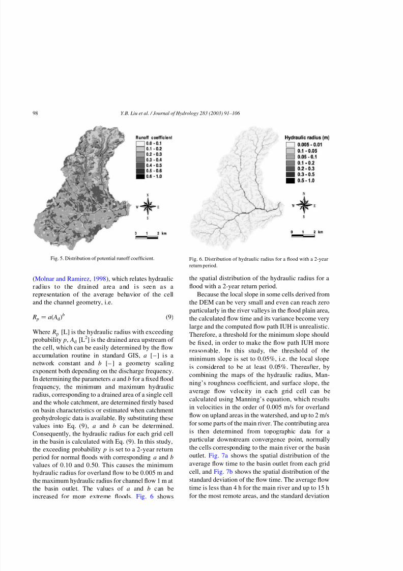
study area is given in Fig. 5.

For calculation of the spatially distributed flow

velocity and dispersion coefficient, both parametersare assumed to depend on local slope, hydraulic radius

and vegetation type. This differs from previous work,

where the flow velocity and dispersion coefficient are

considered to be uniform distributed over the hillslope

and the channel networks and estimated by model

calibration (Van Der Tak and Bras, 1990; Troch et al.,

1994; Gyasi-Agyei et al., 1996; Olivera and Maid-

ment, 1999). In this study, the roughness coefficients

for river courses and different land uses are obtained

from literature (Chow, 1964; Yen, 1991; Ferguson,

1998), while the hydraulic radius is determined by a

power law relationship with an exceeding probabilityFig. 4. Land use map of the study area.

Fig. 3. DEM of the study area.




(Molnar and Ramirez, 1998), which relates hydraulic

r adius t o t he drained area and i s s een as a

representation of the average behavior of the cell

and the channel geometry, i.e.

R p ¼ að AdÞb ð9Þ

Where Rp [L] is the hydraulic radius with exceeding

probability p; Ad [L2] is the drained area upstream of

the cell, which can be easily determined by the flow

accumulation routine in standard GIS, a [ –] i s a

network constant and b [– ] a geometry scaling

exponent both depending on the discharge frequency.

In determining the parameters a and b for a fixed flood

frequency, the minimum and maximum hydraulic

radius, corresponding to a drained area of a single cell

and the whole catchment, are determined firstly basedon basin characteristics or estimated when catchment

geohydrologic data is available. By substituting these

values into Eq. (9), a and b can be determined.

Consequently, the hydraulic radius for each grid cell

in the basin is calculated with Eq. (9). In this study,

the exceeding probability p is set to a 2-year return

period for normal floods with corresponding a and b

values of 0.10 and 0.50. This causes the minimumhydraulic radius for overland flow to be 0.005 m and

the maximum hydraulic radius for channel flow 1 m at

the basin outlet. The values of a and b can be

increased for more extreme floods. Fig. 6 shows

the spatial distribution of the hydraulic radius for a

flood with a 2-year return period.

Because the local slope in some cells derived from

the DEM can be very small and even can reach zeroparticularly in the river valleys in the flood plain area,

the calculated flow time and its variance become very

large and the computed flow path IUH is unrealistic.

Therefore, a threshold for the minimum slope should

be fixed, in order to make the flow path IUH more

reasonable. In this study, the threshold of the

minimum slope is set to 0.05%, i.e. the local slope

is considered to be at least 0.05%. Thereafter, by

combining the maps of the hydraulic radius, Man-

ning’s roughness coefficient, and surface slope, the

average flow velocity in each grid cell can be

calculated using Manning’s equation, which resultsin velocities in the order of 0.005 m/s for overland

flow on upland areas in the watershed, and up to 2 m/s

for some parts of the main river. The contributing area

is then determined from topographic data for a

particular downstream convergence point, normally

the cells corresponding to the main river or the basin

outlet. Fig. 7a shows the spatial distribution of the

average flow time to the basin outlet from each grid

cell, and Fig. 7b shows the spatial distribution of the

standard deviation of the flow time. The average flow

time is less than 4 h for the main river and up to 15 h

for the most remote areas, and the standard deviation

Fig. 6. Distribution of hydraulic radius for a flood with a 2-year

return period.

Fig. 5. Distribution of potential runoff coefficient.




increases with flow length up to 5 h for the most

remote cells. With the above information, the flow

path unit response functions are calculated for each

grid cell to the basin outlet using Eq. (6), and the

watershed unit response function can be calculated

using Eq. (8), weighted by the spatially distributed

runoff coefficient. The calculated watershed IUH is

shown in Fig. 10b.

The generation of surface runoff is performed

using the WetSpa (Water and Energy Transfer

between Soil, Plants and Atmosphere) model

developed by Wang et al. (1996), De Smedt et al.

(2000) and Liu et al. (2002), in which the runoff

production in the cell is calculated by the method of

default runoff coefficients and controlled by the

rainfall intensity and the soil moisture content. A

linear relationship is assumed between the actual

surface runoff and the soil moisture content in the

root zone, where wet soils tend to generate more

runoff and dry soils tend to generate less or even no

runoff. The soil moisture content in each cell is

further simulated on the basis of a soil waterbalance on hourly time scale, which relies on the

rate of the infiltration, percolation, interflow and

evapotranspiration in and out of the root zone.

Finally, the hydrograph at the basin outlet is

obtained by the convolution integral of the excess

precipitation and the flow path IUH from all cells in

the watershed with Eq. (7).

In order to evaluate the performance of the

diffusive wave approximation method for the routing

of surface runoff, 30 months observed hourly

discharge data at the Ell station in the Attert

catchment are selected for the model verification.

The baseflow is separated from the total hydrographby the nonlinear reservoir algorithm (Wittenberg and

Sivapalan, 1999), in which the baseflow is assumed to

be proportional to the square of the groundwater

storage as

Qg ¼ kS 2 ð10Þ

where Qg [L3T21] is the baseflow, S [L] is the

groundwater storage, and k [LT21] is a reservoir

recession coefficient, which is related to the area,

shape, pore volume and transmissivity of the

watershed, and can be derived from the analysis of

the recession curves. Combined with the soil waterbalance equation, the groundwater storage can be

determined and used for baseflow separation with

Eq. (10). It turns out that the computed surface

runoff hydrographs compared very well with the

observations. As a typical example, we show the

results for a flood event that occurred from October

23 to November 13, 1998, shown in Fig. 8, where

the baseflow volume takes about 69% of the totalflood volume, and the direct flow about 31%. The

diffusive flow routing model is then applied with

spatially distributed excess rainfall as input and the

hydrograph at t he bas in out let as output .

Fig. 7. (a) Average flow time to the basin outlet and (b) its standard

deviation.




The predicted direct flow plus baseflow versus

observed hydrograph is shown in Fig. 8 for thesame period. The maximum recorded rainfall

intensity during this period is 12 mm/h, yielding

an observed peak discharge of 29.8 m3 /s, while the

simulated peak flow is 31.4 m3 /s. As can be seen in

the figure, the predicted hydrograph is in good

agreement with the observations.

The results for other periods of the 30 months

observation series are similar. A scatter plot of

observed versus simulated peak direct discharges of

the 24 largest storm events that occurred during the 30

months simulation period are presented in Fig. 9, in

which the measured peak direct discharge is given asthe observed peak discharge minus the baseflow. As

can be seen in the figure, peak floods are reproduced

fairly well, while the low floods tend to be somewhat

overestimated by the model. This is because the

frequency used to estimate the hydraulic radius in the

model is a 2-year return period, which may not be

correct for simulating more frequent flood events. For

assessing the model performance, three evaluation

criteria were applied to the simulation results for the

whole simulation period: (1) the model reproduces the

volume of surface runoff with 8% under estimation,

(2) the model Nash–Sutcliffe efficiency (Nash and

Sutcliffe, 1970) for reproducing the direct discharges

is 83%, and (3) the average correlation coefficientbetween the measured and predicted hydrograph is

76%. Also, the prediction errors of the time to the

peak of the 24 flood events are within 3 h, which

Fig. 8. Observed and predicted stream flow and baseflow separation at Ell station.

Fig. 9. Measured vs. simulated peak direct discharge for a storm

event.




proves that the diffusive transport model is very well

suited for flood prediction in the Attert basin.

4. Sensitivity analysis

The basic purpose of the sensitivity analysis is to

determine differences in the model responses as a

result of changes in the values of specific parameters.

In the present study, a sensitivity analysis wasconducted for the hydraulic radius, the channel

roughness coefficient, the threshold for minimum

slope, and the area threshold in delineating channel

networks. The sensitivity results are, however, site

specific and may vary with locations of different

catchment size, soils, land use, and slope configur-

ations. The effect of each parameter is studied byvarying its value while keeping other parameters

constant. In all cases, the predicted hydrograph for a

flood event in October 1998 is considered as

references. The calculated watershed IUH by Eq. (8)

is also presented to give a graphical view of the effect

on the mean, variance and skewness of the averagetravel time, even though it is not used to calculate the

outlet hydrograph.

4.1. Effect of hydraulic radius

Instead of using a constant hillslope velocity and

channel flow velocity to calculate the flow path

response and watershed response as in many of the

previous works, the concept of minimum energy

expenditure is applied here to derive the hydraulic

radius. The flow velocity is considered to be location

dependent relying on the roughness coefficient, the

local slope, and the hydraulic radius. The averagehydraulic radius is obtained by the power law

relationship given by Eq. (9) (Molnar and Ramirez,

1998), which is assumed to be constant for a flood

event, but may vary from event to event according to

the flood frequency.

Three flood frequencies, namely 0.1, 0.5 and 2.0,

were considered to study their influence on the runoff

hydrograph at the outlet and the watershed IUH, while

keeping other parameters constant. The frequencies,

0.1, 0.5 and 2.0, correspond to return periods of 10, 2

and 0.5 years, respectively. The corresponding values

of calculated hydraulic radius at the basin outlet are

about 1.5, 1.0 and 0.5 m, respectively, while the

minimum value of the hydraulic radius remain

constant at 5 mm for surface runoff in the upstream

part of the catchment. It is found from Fig. 10a that a

change in the flood frequency causes a considerable

alteration in the peak value of the simulated direct

hydrographs and the catchment IUH. The peak

discharge increases from 16.7 to 17.8 m3 /s and shifts

1 h ahead as the flood frequency decreases from 0.5 to

0.1, and decreases to 14.7 m3

/s with 1 h time delay asthe flood frequency increases to 2.0. This is logical

because big storms lead to higher peak discharges and

shorter travel times. Fig. 10b shows the effect of the

hydraulic radius on the calculated watershed IUH.

The mean, variance and the skewness of the travel

Fig. 10. (a) Simulated direct hydrographs and (b) calculated

watershed IUH showing the effect of hydraulic radius with expected

frequency, p:




time are decreasing with increased flood frequency,

because these parameters are inversely depending on

the celerity, as can be seen from Eqs. (3)–(5), and any

increase in hydraulic radius will result in less damping

and faster response of the flood wave.

4.2. Effect of channel roughness

Since surface runoff from each grid cell will

contribute to the stream flow, the roughness coeffi-cient has a direct impact on the travel time and amount

of dissipation that will occur when routing a flood

hydrograph through a river basin. Roughness coeffi-

cients for hydrologic routing models are typically in

the form of Manning’s n values, and estimated based

on the channel geometry. Generally, the roughness

coefficient is higher for upstream channels, and

decreases with stream order when the channel slopebecomes small. For the convenience of model

computation and result comparison, the channel

roughness coefficient is considered to be constant in

this example regardless of the effect of stream order.

Fig. 11a shows the simulated direct runoff hydro-graphs and the calculated watershed IUH with three

different values of Manning’s roughness coefficient.

The value 0.03 corresponds to clean and straight

streams without riffles or deep pools, 0.04 to clean and

winding streams with some pools and shoals, and 0.05

to clean and winding streams with stones (Chow,

1964). It is found that the peak discharge decreases

from 16.7 to 14.3 m3 /s and is somewhat delayed as the

roughness coefficient increases from 0.04 to 0.05, and

increases to 20.2 m3 /s with 1 h shifting ahead as the

roughness coefficient decreases to 0.03. Since the total

runoff volume remains constant, reduction in peak

discharge and delay in peak time are compensated byprolonged flow recession, and vice versa. This is also

reflected in the calculated watershed IUH as shown in

Fig. 11b. The mean, variance and the skewness of the

travel time are increasing with increasing roughness,

due to the fact that any increase in roughness

coefficient will result in higher shear stresses, causing

more damping and slowing down of the flood wave.

4.3. Effect of minimum slope

The present approach considers the changes in

velocity with respect to distance, but ignores

the changes in velocity with respect to time. There-

fore, it can be used to route slow rising floodwavesthrough very flat slopes, but errors in the amount of

damping will occur when routing rapidly rising flood

waves through extremely flat channel slopes, because

the inertia terms are not included in the diffusion wave

method. In GIS, the slope of the cell is derived from

the DEM and calculated from the 3 £ 3 neighbour-

hood using the average maximum technique. Inevi-

tably, nearly zero slopes may occur in some areas,

especially in the river valleys in the flood plain area,

resulting in nearly infinity travel time and damping.

To mitigate the impact of the extremely flat slopes on

the flow path function, it is necessary to import


watershed IUH showing the effect of channel Manning’s roughness

coefficient, n:




a threshold for minimum slope, i.e. the cell slope is

put equal to the threshold value when the calculated

slope is smaller than the threshold.

Keeping all other parameters constant, three values

of minimum slope, namely, 0.01, 0.05 and 0.1% are

considered to study the effect of the threshold value on

the outflow hydrograph and the calculated watershed

IUH. Results are shown in Fig. 12a and b. It is found

that the peak discharge and the time to the peak of the

watershed IUH decrease slightly with a smallerthreshold for minimum slope. This is because a

decrease in slope will reduce the flood wave celerity,

and therefore increase the travel time and the amount

of hydrograph attenuation. Since the number of cells

with a slope lower that the thresholds is small in this

catchment, the influence of the minimum slope is not

very significant as can be seen in the figure. However,

the minimum slope may have a large influence on the

outflow hydrograph for catchments with flatter slopes.

4.4. Effect of area threshold in delineating

channel networks

In standard GIS applications, such as ArcInfo andArcView, watershed channels are delineated based on

the upstream area of each cell. It is assumed that any

upstream area smaller than the threshold value does

not produce enough runoff to support a channel. The

area required to develop a channel depends on

regional and watershed characteristics such as cli-

matic conditions, soil properties, surface cover, and

slope characteristics (Martz and Garbrecht, 1992). Incells that are not part of the stream network, overland

flow occurs. Therefore, with a small area threshold

value, GIS derived stream networks are more

meticulous and may represent ephemeral and inter-

mittent streams that are too small to be represented ontopographical maps.

The effect of the area threshold in delineating

channel networks on the outflow hydrograph and the

calculated watershed IUH is investigated by varying

the cell number threshold, namely 5, 10 and 50, which

corresponds to draining areas of, respectively, 12,500,

25,000 and 125,000 m2, while keeping other model

parameters constant. It can be seen from Fig. 13a

and b, that there is no significant effect on the peak

discharge and the calculated watershed IUH in this

catchment. This is due to the fact that changes in the

threshold area will result in expansion or shrinking of

the stream network with lengths that are, however,relatively short compared to the whole flow paths.

Hence, the impact will only become significant when

using large threshold values, because in this case

hillslope effects become important due to their high

overland flow roughness, which will result in a longer

flow time, and a prolonged flow response at the end of

the flow path.

4.5. Other effects

In addition to the effects discussed above, the

variation of channel geometry and the temporal and


watershed IUH showing the effect of the threshold of minimum

slope, S min:




spatial resolutions of the model will also have

considerable influence on the outflow hydrographand the watershed IUH. In this study, flow is routed

using a velocity calculated for each land use category

both for overland flow and channel flow. The velocity

is determined from Manning’s equation by assuming

that the hydraulic radius equals the average flow depth

without considering the effect of channel width and

type. This assumption is warranted if the width of the

river is much larger than its depth for a flood event.

However, as the width of a channel decreases, the

hydraulic radius does not tend towards the average

flow depth. Also, the effect of flood plains on the

propagation of a floodwave can be very significant,

when water overflows the riverbanks. It is expected

that an expanded channel width will slow down the

flow velocity and therefore reduce the peak discharge

and delay the resulting runoff hydrograph. Hence,

more reliable results can be obtained when calculating

the hydraulic radius combined with measured or

estimated channel width.

The time and space scale of the model not only

influence on rainfall intensity and the surface runoff

distribution, but they also have impacts on thewatershed IUH derived from the diffusive transport

method. Errors may arise when modeling flash flood

for a small catchment with a long time scale. This is

because floodwater can flow out of the catchment

within the first time step, which the IUH cannot

calculate accordingly. Therefore, a lower time

resolution is necessary in this case. However, when

modeling floods in a large catchment with relatively

long concentration times, the effect of time scale is not

important. On the other hand, changes in spatial

resolution of the model will lead to variations of the

GIS derived slope, flow direction, and spatial

distribution of the flow paths. In general, higher

spatial resolution tends to generate longer flow paths,

and hence increases the hydrodynamic and the

geomorphologic attenuation of the flood wave. The

first is due to increased flow time, and the second to

increased variability of the flow paths. Both impacts

will play an important role in the prediction of

transport phenomena, especially in large basins

(Rinaldo et al., 1991). It is expected that reduction

in the spatial resolution will result in a decrease of

peak discharge and prolonged time to flood peaks, and

vice versa.

As pointed out by Horritt and Bates (2001), a high-resolution model is advantageous when small scale

processes have a significant effect on model predic-

tions, but have to be balanced against the increased

computation onus. Predictions with a low-resolution

may also give an essentially correct result in many

cases. In practice, determination of temporal and

spatial resolution of the model should rely on the data

available, the catchment characteristics and the model

accuracy requirement. However, quantitative analysis

of these effects on the outflow hydrograph and the

watershed IUH in GIS flood modeling is beyond the

scope of this paper.


watershed IUH showing the effect of area threshold in delineating

channel networks with cell number threshold, C n:




5. Conclusions

A physically based distributed unit hydrograph

method derived from the diffusive transport approach

is presented in this paper for GIS based modeling on

catchment scale. The method differs from the previous

work in that it is based on a location dependent

velocity field. The basic modeling approach is to use

raster GIS functions to calculate the travel time from

each point in the watershed to the outlet bydetermining the flow path and the travel time through

each cell along the path. The flow velocity in each grid

cell is calculated by the Manning equation, which

depends upon the local slope, roughness coefficient

and hydraulic radius. The travel time through each

individual cell along the flow path is integrated to

obtain the cumulative travel time to the outlet. Based

on the mean and the variance of the flow time, the first

passage time distribution density function is applied

as a flow response function. Runoff is routed over the

surface flow path, and accounts for the differences in

runoff amount and velocity, due to changing slope,

land use, soil type and other surface conditions.Finally, the total direct discharge at the downstream

convergence point is obtained by superimposing allcontributions from every grid cell. The watershed

IUH is calculated based on the flow path functions and

the spatially distributed runoff coefficient, and can be

used for model parameter sensitivity analysis or as the

IUH for lumped prediction models. Model parameters

based on surface slope, land use, soil type and their

combinations are collected from literature, and can be

prepared easily using standard GIS techniques.

The model was tested on the Attert catchment in

Luxembourg with 30 months of observed hourly

rainfall and discharge data, where the spatial dis-tributed surface runoff was generated by the WetSpa

model. The results show an excellent agreement with

the measured hydrograph at the basin outlet. Conse-

quently, a sensitivity analysis was conducted to study

the effect of the hydraulic radius, the channel

roughness coefficient, the threshold for minimum

slope, and the area threshold in delineating channel

networks on the outflow hydrograph and the calcu-

lated watershed IUH. It was found that the hydraulic

radius and channel roughness coefficient are the most

sensitive parameters. The hydraulic radius corre-

sponding to a 2-year return period can meet

the requirements of flood prediction for normal floods,

but should be increased for more extreme flood. Also,

the channel roughness coefficient shows a strong

impact on the model output. More reliable results are

expected when the channel roughness is determined

according to the stream order. The thresholds of

minimum slope and the area in delineating channel

networks have only marginal effects on the outflow

hydrograph and the calculated watershed IUH.

However, all these parameters should be chosenproperly when applying the model in practice.

The diffusive wave transport approach assumes a

unique relationship between flow and stage at each

point for both overland flow and channel flow, and so

does not require the specification of a downstream

stage. It also generally operates satisfactorily with less

detailed ditch and channel geometry information than

required by dynamic wave models and is much more

stable and easy to use in GIS based flood modeling.

Moreover, this approach allows the spatially distrib-

uted excess precipitation and hydrologic parameters

of the terrain to be used as inputs to the model, and is

especially useful to analyze the effects of topography,and land use or soil cover on the hydrologic behavior

of a river basin. The method is worth to be applied in

flood modeling for a wide range of slopes from flood

plains to the hilly areas. However, accuracy of the

diffusive wave approach increases with increasing

slope, and it cannot be used in situations where flow

reversals occur. Application of the methodology

suggests that simulations of the hydrologic response

based on diffusive wave approximation and GIS

specification of the topographical network are vali-

dated in the study area. This is sustained by a proper

adjustment of the parameter values characterizing the

flow travel time and its variance, which is deemed to

cover most cases of engineering interest.

References

Beven, K.J., Kirkby, M.J., 1979. A physically based variable

contributing area model of basin hydrology. Hydrol. Sci. Bull.

24 (1), 43–59.

Browne, F.X., 1990. Stromewater management. In: Corbitt, R.A.,

(Ed.), Standard Handbook of Environmental Engineering,

McGraw-Hill, New York, pp. 7.1–7.135.

Chow, V.T. (Ed.), 1964. Handbook of Applied Hydrology,

McGraw-Hill Book Company, New York, pp. 7–25.




Chow, V.T., Maidment, D.R., Mays, L.W., 1988. Applied

Hydrology, McGraw-Hill, New York.

Cunge, J.A., Holly, F.M., Verwey, A., 1980. Practical Aspects of

Computational River Hydraulics, Pitman, London, GB, p. 45.

De Groot, M.H., 1986. Probability and Statistics, Addison-Wesley,

Reading, MA, USA.

De Smedt, F., Liu, Y.B., Gebremeskel, S., 2000. Hydrologic

modeling on a catchment scale using GIS and remote sensed

land use information. In: Brebbia, C.A., (Ed.), Risk Analysis II,

WTI press, Southampton, Boston, pp. 295–304.

Dooge, J.C.I., 1959. A general theory of the unit hydrograph.

J. Geophys. Res. 64, 241–256.

Eagleson, P.S., 1970. Dynamic Hydrology, McGraw-Hill, New

York, p. 364.

Ferguson, B.K., 1998. Introduction to Stormwater, Concept,

Purpose and Design, Wiley, New York, p. 111.

Gupta, V.K., Waymire, E., 1983. On the formulation of an

analytical approach to hydrologic response and similarity at

the basin scale. J. Hydrol. 65, 95–123.

Gupta, V.K., Waymire, E., Wang, C.T., 1980. A representation of

an instantaneous unit hydrograph from geomorphology. Water

Resour. Res. 16 (5), 855–862.

Gyasi-Agyei, Y., De Troch, F.P., Troch, P.A., 1996. A dynamic

hillslope response model in a geomorphology based rainfall–

runoff model. J. Hydrol. 178, 1–18.

Henderson, F.M., 1966. Open Channel Flow, McMillan, New York,

p. 522.

Horritt, M.S., Bates, P.D., 2001. Effect of spatial resolution on a

raster based model of flood flow. J. Hydrol. 253, 239–2498.

Kirkby, M.J. (Ed.), 1978. Hill-slope Hydrology, Wiley, p. 235.

Lee, K.T., Yen, B.C., 1997. A geomorphology and kinematic-wave-

based hydrograph derivation. J. Hydraulic Engng., ASCE 123

(1), 73–80.

Liu, Y.B., Gebremeskel, S., De Smedt, F., Pfister, L., 2002. Flood

prediction with the WetSpa model on catchment scale. In: Wu,

et al. (Eds.), Flood Defence’2002, Science Press, New York, pp.

499–507.

Maidment, D.R., 1993. Developing a spatially distributed unit

hydrograph by using GIS. In: Dovar, K., Natchnebel, H.P.

(Eds.), Application of Geographic Information Systems in

Hydrology and Water Resources, Proceedings of the ViennaConference, Vienna: Int. Assoc. of Hydrological Sci., pp.

181–192.

Maidment, D.R., Olivera, J.F., Calver, A., Eatherral, A., Fraczek,

W., 1996. A unit hydrograph derived from a spatially distributed

velocity field. Hydrol. Process 10 (6), 831–844.

Mallants, D., Feyen, J., 1990. Kwantitatieve en kwalitatieve

aspecten van oppervlakte en grondwaterstroming (in Dutch),

vol. 2. KUL, p. 96.

Martz, L.W., Garbrecht, J., 1992. Numerical definition of drainage

network and subcatchment areas from digital elevation models.

Comput. Geosci. 18 (6), 747–761.

Mesa, O.J., Mifflin, E.R., 1986. On the relative role of hillslope and

network geometry in hydrologic response. In: Gupta, V.K.,

Rodriguez-Iturbe, I., Wood, E.F. (Eds.), Scale Problems in

Hydrology, D. Reidel, Norwell, Mass, pp. 1–17.

Molnar, P., Ramirez, J.A., 1998. Energy dissipation theories and

optimal channel characteristics of river networks. Water Resour.

Res. 34 (7), 1809– 1818.

Naden, P.S., 1992. spatial variability in flood estimation for large

catchments: the exploitation of channel network structure.J. Hydrol. Sci. 37, 53–71.

Nash, J.E., Sutcliffe, J.V., 1970. River flow forecasting through

conceptual models. J. Hydrol. 10, 282–290.

Olivera, F., Maidment, D.R., 1999. Geographic information system

(GIS)-based spatially distributed model for runoff routing.

Water Resour. Res. 35 (4), 1155–1164.

Pfister, L., Humbert, J., Hoffmann, L., 2000. Recent trends in

rainfall–runoff characteristics in the Alzette river basin,

Luxembourg. Climate Change 45 (2), 323–337.

Pilgrim, D.H., Cordery, I., 1993. Flood runoff. In: Maidment, D.R.,

(Ed.), Handbook of Hydrology, McGraw-Hill, New York, pp.

9.1–9.42.

Rinaldo, A., Marani, A., Rigon, R., 1991. Geomorphological

dispersion. Water Resour. Res. 27 (4), 513–525.

Rodriguez-Iturbe, I., Valdes, J.B., 1979. The geomorphologic

structure of hydrologic response. Water Resour. Res. 15 (6),

1409–1420.

Sivapalan, M., Wood, E.F., Beven, K., 1990. On hydrologic

similarity. 3. A dimensionless flood frequency model using a

generalized geomorphologic unit hydrograph and partial area

runoff generation. Water Resour. Res. 26 (1), 43–58.

Snell, J.D., Sivapalan, M., 1994. On geomorphological dispersion in

natural catchments and the geomorphological unit hydrograph.

Water Resour. Res. 30 (7), 2311–2323.

Troch, P.A., Smith, J.A., Wood, E.F., de Troch, F.P., 1994.

Hydrologic controls of large floods in a small basin. J. Hydrol.

156, 285–309.

Van Der Tak, L.D., Bras, R.L., 1990. Incorporating hillslope effects

into the geomorphological instantaneous unite hydrograph.

Water Resour. Res. 26 (1), 2393–2400.

Wang, Z., Batelaan, O., De Smedt, F., 1996. A distributed model forwater and energy transfer between soil, plants and atmosphere

(WetSpa). Phys. Chem. Earth 21 (3), 189–193.

Wittenberg, H., Sivapalan, M., 1999. Watershed groundwater

balance estimation using streamflow recession analysis and

baseflow separation. J. Hydrol. 219, 20–33.

Yen, B.C. (Ed.), 1991. Channel Flow Resistance: Centennial of

Manning’s Formula, Water Resources Publications, Littleton,

CO, p. 43.


Date post:	07-Apr-2018
Category:	Documents
Upload:	sudharsananprs
View:	225 times
Download:	0 times

Diffusive Transport Approach

Documents