1 DIGITAL MAP OF SURFICIAL GEOLOGY, WETLANDS, AND DEEPWATER HABITATS, COEUR D’ALENE RIVER VALLEY, IDAHO by Arthur A. Bookstrom 1 , Stephen E. Box 1 , Berne L. Jackson 3 , Theodore R. Brandt 2 , Pamela D. Derkey 1 , and Steven R. Munts 4 Open-File Report 99-548 1999 Prepared in cooperation with the Coeur d’Alene Tribe This report is preliminary and has not been reviewed for conformity with U.S. Geological Survey editorial standards or with the North American Stratigraphic Code. Any use of trade, firm, or product names is for descriptive purposes only and does not imply endorsement by the U.S. Government. U.S. DEPARTMENT OF THE INTERIOR U.S. GEOLOGICAL SURVEY 1 USGS, Spokane, WA 99201, 2 USGS, Denver, CO 80225, 3 Coeur d’Alene Tribe, Plummer, ID 83851, 4 Information Systems Support, Inc., Spokane, WA 99201
Transcript
1
DIGITAL MAP OF SURFICIAL GEOLOGY, WETLANDS, AND DEEPWATER HABITATS, COEUR D’ALENE RIVER VALLEY, IDAHO by Arthur A. Bookstrom1, Stephen E. Box1, Berne L. Jackson3, Theodore R. Brandt2, Pamela D. Derkey1, and Steven R. Munts4 Open-File Report 99-548 1999 Prepared in cooperation with the Coeur d’Alene Tribe
This report is preliminary and has not been reviewed for conformity with U.S. Geological Survey editorial standards or with the North American Stratigraphic Code. Any use of trade, firm, or product names is for descriptive purposes only and does not imply endorsement by the U.S. Government. U.S. DEPARTMENT OF THE INTERIOR U.S. GEOLOGICAL SURVEY 1 USGS, Spokane, WA 99201, 2 USGS, Denver, CO 80225, 3 Coeur d’Alene Tribe, Plummer, ID 83851, 4 Information Systems Support, Inc., Spokane, WA 99201
2
This page is left blank intentionally, as the back of the cover page for two sided printing.
3
CONTENTS
ABSTRACT 7
INTRODUCTION 8
Purpose 8
Map of Surficial Geology, Wetlands, and Deepwater Habitats 9
Location and Setting 10 Coeur d’Alene River Basin 10 Coeur d’Alene River Valley 10 Coeur d’Alene Mining District 16 Post Falls Dam 17 Floods 17 Metal-Enriched Sediments 19
Methods 23
MAP OF SURFICIAL GEOLOGY, WETLANDS, AND DEEPWATER HABITATS 27
Map-Unit Names and Symbols 28
DESCRIPTION OF MAP UNITS 32
Highland System 34
Upper Perennial Subsystem 36 Riverine Features, Upper Perennial Subsystem 39 Upland Features of the Terraced Floodplain 40 Palustrine Habitats of the Terraced Floodplain 41
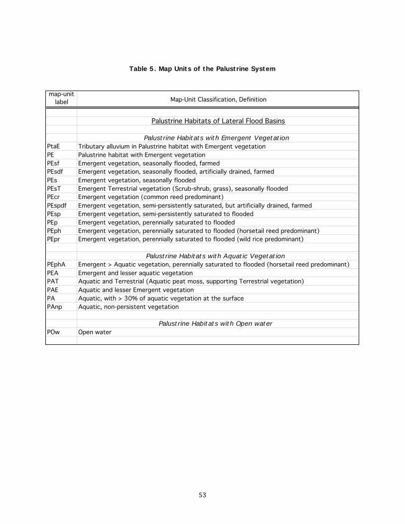
Palustrine Habitats of Lateral Flood Basins 52 Palustrine Habitats with Emergent Vegetation 54 Palustrine with Aquatic Vegetation 55 Palustrine Habitat with Open Water 56
Lacustrine Habitats of Lateral Flood Basins 56 Map Units of the Lacustrine Littoral Subsystem 58 Map Units of the Lacustrine Limn etic Subsystem 58
Deltaic Features and Environments 59
4
Deltaic Features in Lateral Lakes 59 Deltaic Features at the Mouth of the CdA River, in CdA Lake 59
FIGURES Figure 1. Index and Location Maps, Coeur d’Alene (CDA) River and other Major Tributaries of the Spokane River Basin 11 Figure 2. Index and Location Maps, CDA Lake, CDA River, CDA Mining District,
And Bunker Hill Superfund Site 12 Figure 3. Location Map, Upper CDA River Valley 13 Figure 4. Location Map, Middle CDA River Valley 14 Figure 5. Location Map, Lower CDA River Valley 15 Figure 6. Lead-Concentration Profiles in Metal-Enriched Sediments 20 Figure 7. Block Diagram, Braided Gravel-Bottomed River and Alluvial Terraces, Confluence to Cataldo Landing 37 Figure 8. Block Diagram, Sand-Bottomed Meandering River, Cataldo Landing To Harrison 43
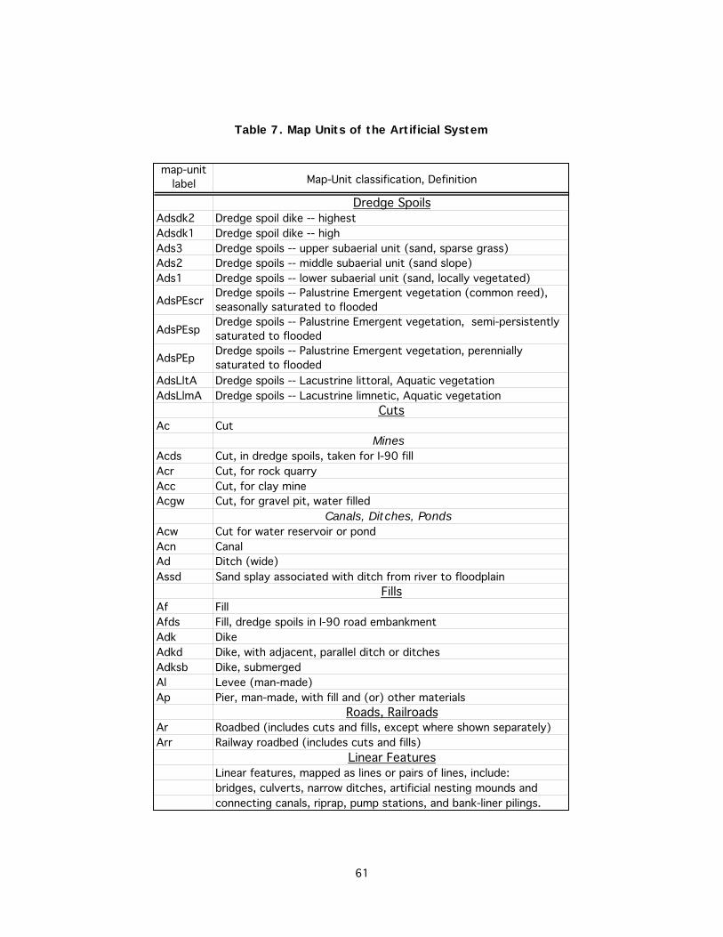
TABLES Table 1. Classification of Map-Unit Names and Symbols 29 Table 2. Map Units of the Highland System 33 Table 3. Map Units of Upper Perennial Riverine, Upland and Palustrine Features 38 Table 4. Map Units of Lower Perennial Riverine, Trans-Floodplain and Upland Features 44 Table 5. Map Units of the Palustrine System 53 Table 6. Map Units of the Lacustrine System 57 Table 7. Map Units of the Artificial System 61 Table 8. Thematic Attributes of Map Units, CDA River Valley 67
6
7
Abstract In north Idaho the Coeur d’Alene (CdA) River channel and its floodplain are
mostly covered by metal-enriched sediments, partially derived from upstream mining, milling and smelting wastes. Relative to uncontaminated sediments of the region, metal-enriched sediments are highly enriched in silver, lead, zinc, arsenic, antimony and mercury; and enriched in copper, cadmium, manganese, and iron (Fousek, 1996). Widespread distribution of metal-enriched sediments has resulted from over a century of mining in the CdA mining district (upstream), poor mine-waste containment practices during the first 80 years of mining, and an ongoing series of over-bank floods. Previously deposited metal-enriched sediments continue to be eroded and transported down-valley and onto the floodplain during floods.
The centerpiece of this report is a Digital Map Surficial Geology, Wetlands and Deepwater Habitats of the Coeur d’Alene (CdA) River valley (sheets 1 and 2). The map covers the river, its floodplain, and adjacent hills, from the confluence of the North and South Forks of the CdA River to its mouth and delta front on CdA Lake, 43 linear km (26 mi) to the southwest (river distance 58 km or 36 mi). Also included are the following derivative theme maps: 1. Wetland System Map, 2. Wetland Class Map, 3. Wetland Subclass Map, 4. Floodplain Map, 5. Water Regime Map, 6. Sediment-Type Map, 7. Redox Map, 8. pH Map, and 9. Agricultural Land Map.
The CdA River is braided and has a cobble-gravel bottom from the confluence to Cataldo Flats, 8 linear km (5 mi) down-valley. Erosional remnants of up to four alluvial terraces are present locally, and all are within the floodplain, as defined by the area flooded in February of 1996. High-water (overflow) channels and partly filled channel scars braid across some alluvial terraces, toward down-valley marshes and (or) oxbow ponds, which drain back to the river.
Near Cataldo Flats, the river gradient flattens, and the river coalesces into a single channel with a large friction-dominated central sand bar at Cataldo Landing. Metal-enriched sediments that were dredged from the central sand bar were deposited on Cataldo Flats, to form extensive dredge-spoil deposits. From the central sand bar to CdA Lake, thick deposits of metal-enriched sand partially fill the middle of the pre-mining-era channel along straight reaches, and form point-bars along the inside margins of meander bends. Metal-enriched sand and silt form oxidized bank-wedge deposits along riverside margins of pre-mining-era levees of gray silty mud. Metal-enriched levee sand deposits extend across bank wedges and natural levees, generally thinning and fining away from the river, toward lateral marshes and lakes, where dark gray metal-enriched silt and mud overlie silty peat, deposited before the mining era. Distributary streams and man-made canals locally diverge from the river, connecting it to lateral marshes and lakes, and metal-enriched sand splays locally fan out across the floodplain. At the mouth of the river, a bouyancy-dominated river-mouth bar crests beyond the ends of the emergent levees. Thick delta-front deposits of metal-enriched sand slope from the river-mouth bar to the bottom of CdA Lake.
8
Introduction A Digital Map of Surficial Geology, Wetlands, and Deepwater Habitats of the
Coeur d’Alene (CdA) River valley (sheets 1 and 2) is the centerpiece of this report. The map depicts the CdA River, its floodplain, the hills and valleys adjacent to the floodplain. The map area extends from the confluence of the North and South Forks of the CdA River, to its river-mouth bar and delta front at the junction of the Harrison and St. Joe Arms of CdA Lake. This report explains why and how the Digital Map of Surficial Geology, Wetlands and Deepwater Habitats (sheets 1 and 2) was made. It defines and explains the features, materials, and environments represented by the map units. It also includes a table of information that makes possible the derivation of nine or more thematic maps. Sheets 3 to 6 characterize areas represented by map units in terms of Wetlands System, Class, Sub-class and Water Regime, as defined by Cowardin and others (1979). Sheets 7 defines the extent of the floodplain, sheet 8 shows distributions of expected sediment types, sheets 9 and 10 map expected redox and pH conditions in metal-enriched sediments, and sheet 11 indicates areas that are agriculturally cultivated.
Sheets 1 through 11 are colored digital maps. They are not available in paper form, but instructions for obtaining them via the Internet, viewing them on-screen, and making paper copies from the digital files are included in Appendices B, C, and D of this report.
Purpose
The purpose of this report and its accompanying maps is to delineate and describe the distribution of surficial features and materials in and around the floodplain of the CdA River valley, which is mostly covered with metal-enriched sediment, water and vegetation. These maps are intended as base maps on which to compile additional geochemical, biologic and engineering information. Through interactive analysis of such data in the context of the information on these base maps, we hope to better understand the physical and chemical processes involved in the distribution, temporary storage, and continuing re-distribution of metal-enriched sediments that cover most of the valley floor. We hope that improved understanding of processes acting on the metal-enriched sediments will be applied to the search for remedial and restoration strategies that will be effective over the long term.
This map and report are offered as contributions to the following environmental
remediation and restoration efforts in the CdA River valley:
1) Natural Resource Damage Assessment and Restoration (NRDAR) by U.S. Fish and Wildlife Service (USFWS), Coeur d’Alene Tribe, U.S. Bureau of Land Management (USBLM), and U.S. Department of Agriculture - Forest Service (USFS);
2) Remedial Investigation/Feasibility Study (RI/FS) and Conceptual Site Model (CSM) by U.S. Environmental Protection Agency (EPA); and
9
3) Environmental studies and remediation activities by Silver Valley Natural Resource Trustees, Idaho Department of Environmental Quality (DEQ), Idaho Department of Fish and Game, and
4) Other public and private efforts to improve environmental conditions in the CdA River valley.
Map of Surficial Geology, Wetlands, and Deepwater Habitats
Surficial geology is the geology of surficial deposits, including unconsolidated and residual, alluvial or glacial deposits, soil, and bed-rock, as seen at the Earth’s surface (Bates and Jackson, 1987). Wetlands are lands where saturation with water is the dominant factor determining the nature of soil development and the types of plant and animal communities living in the soil and on its surface (Cowardin and others, 1979). Deepwater habitats are permanently flooded lands lying below the deepwater boundary of wetlands, so that water, rather than air is the principal medium within which the dominant organisms live, whether or not they are attached to the substrate (Cowardin and others, 1979).
The Map of Surficial Geology, Wetlands, and Deepwater Habitats (sheets 1 and 2) is a hybrid map. It shows surficial geological features where they are exposed or known from drill holes or geophysical surveys, or indicated by geological interpolation or extrapolation. In areas that are covered by water and (or) vegetation the map shows wetland and deepwater habitats, classified in accordance with the “Classification of Wetlands and Deepwater Habitats of the United States” by Cowardin and others (1979). Although surficial geologic features are not directly exposed in those areas, the wetland and deepwater habitats are indicative of environments of sediment transport, deposition and storage in the river and on its floodplain.
Floodplains are nearly flat lowlands that border a stream, and may be covered by its waters at flood stages (Bates and Jackson, 1987). “Flooplains are an important functional part of fluvial systems. They absorb and gradually release floodwaters, filter contaminants from run-off, recharge groundwater, provide diverse wildlife habitats and are sites of sediment accumulation and storage” (Marriott and Alexander, 1999). The floodplain of the CdA River includes the area that was inundated during the flood of February 1996, which had a peak flow of 68,300 ft3/s at Cataldo and drove the level of CdA Lake to the 2,133 ft elevation (8 ft above normal). This is close to the 100-year flood peak of 70,800 ft3/s, as calculated by Beckwith, Berenback and Backson (1996). The winter flood of 1974 had a higher instantaneous peak flow (estimated as 79,000 ft3/s at Cataldo). The winter flood of 1933 (67,000 ft3/s) was more prolonged and drove the level of CdA Lake to its maximum elevation (2,136 ft), 11 ft above summer water level (Data are from Beckwith, Berenbrock and Backson, 1996; Harenberg and others, 1993; and Grover, 1936. Elevations are adjusted to the 2,125 summer-water elevation at the Harrison gage.). However, since we were able to observe the extent and effects of the February 1996 flood, we define the floodplain of the CdA River in terms of the area flooded during that flood.
10
Location and Setting
Coeur d’Alene River Basin The CdA River drains a large part of the north Idaho panhandle, from a divide that defines Idaho’s eastern border, to CdA Lake, near Idaho’s western border (figure 1). The CdA River Basin occupies the western side of the northern Bitterroot Range, between the Clark Fork River Basin to the northeast, and the St. Joe River Basin to the south. The North Fork of the CdA River drains an area of about 900 sq mi, and its average discharge is about 2,000 ft3/s. The South Fork of the CdA River drains an area of about 300 sq mi, and its average discharge is about 500 ft3/s.
The North and South Forks of the CdA River join near Enaville, Idaho, to form the main stem of the CdA River, which meanders about 58 km (36 mi) southwesterly to CdA Lake, near Harrison, Idaho (figures 1 and 2). The area of the Digital Map of Geology and Wetlands of the CdA River Valley, represented in sheets 1 and 2, extends from the confluence of the North and South Forks of the CdA River to its delta front on CdA Lake, near Harrison (figures 2, 3, and 4). Relatively steep gradients of the North and South Forks flatten downstream, and approach a nearly flat gradient from Cataldo Flats to CdA Lake. The cobble-gravel bottom of the river channel upstream from Cataldo Flats gives way to a large central sand bar, which occupies a wide bend in the river channel at Cataldo boat landing. River-bottom sediments are predominantly sandy from there to the toe of the delta front, on CdA Lake.
Coeur d’Alene River Valley
The maps in figures 3, 4 and 5 show the Upper, Middle and Lower segments of the CdA River valley. The transition from braided, gravel-bottomed channel of the Upper Perennial Riverine Subsystem of Cowardin and others (1979) to the meandering, sand-bottomed channel of the Lower Perennial Riverine Subsystem is at Cataldo Flats, in the Upper CdA River valley (figure 3). Most place names shown on figures 3, 4 and 5 are from the following maps: 1) 7.5’ topographic maps of the Cataldo, Rose Lake, Lane, Medimont, Black Lake, and Harrison, Idaho quadrangles (USGS, 1981, 1985); 2) planimetric map of the Idaho Panhandle National Forests (Coeur d’Alene National Forest, Idaho and Montana (USDA Forest Service, 1989); and 3) location map of National Resource Damage Assessment study areas in the CdA River Valley (USFWS, unpub. map, 1998). However, areas or features not labeled on those source maps are assigned the names of corresponding ranches, landowners, or man-made features.
Figure 1. Index and location maps showing the Coeur d'Alene River and other major tributary streams and rivers of the Spokane River Basin (from Woods and Beckwith, 1996). Locations of cities, towns, and the Bunker Hill Superfund Site also are shown.
11
Coeur d'Alene
Smelterville KelloggRose Cataldo
Bunker HillSuperfund Site
Wallace
Osburn
Coeur d'Alene mining district
Mullan47o 30'
Coeur d'Alene Lake
North Fork
Harrison
St. Joe River
Burke
Coeur d'Alene River
SouthForkKingston
Spokane River
0
10
20
River miles below Mullan
6050
40
30
40
Elizabeth Park
o
Post Falls Dam
Wolf Lodge Bay
East Pt.
Gasser Pt.
Fuller's Bay
Coukling Pt.
PinehurstPine Cr.
Figure 2. Index and location maps, showing Coeur d'Alene (CdA) Lake, the CdA River, its North and South Forks, the CdA mining district, and the Bunker Hill Superfund Site.
*
*
* * * * * ***
**
*
Enaville
*
10 Km
10 MiN
OR
MT
WYID
AREA OF MAP
WA
116
Nin
emile
Cr.
Canyon Cr.
City or town site *
Prichard Cr.Murray*
lower
middle
Lake
upper
12
1
4
2
3
47 35'o
47 32' 30"o
1
4
2
3
1
4
2
3
1
4
2
3
Bull Run C
r.
Rose Lake
Rose Lake
Porte
r Slo
ugh
OrlingSlough
Canyon Marsh
Dudley
Dud
ley
M
eado
w
dt Frutchey'sMeadow
MissionSlough
CataldoSlough
Cataldo Lead Flats Kingston
Enaville
upper Coeur d'Alene River valley
*
*
*
ct *
Cat
aldo
Terra
ces
#
Fourth of July Cr.
Nor
th F
ork
South Fork
CdA River
Fren
ch C
r.
2200
2200
22002200
Figure 3. Location map of the upper CdA River valley, showing the river and the 2,200 ft elevation contour along the hillsides that bound the floodplain. Also shown are locations and names of features described in the text: = town, # = sawmill site (abandoned), cl = Cataldo Landing (x), ct = Cataldo drill transect, dt = Dudley drill transect, mb = McPhee Bridge, eb = Enaville Bridge, erb = Enaville railroad bridge, crb = Cataldo railrooad bridge, chb = Cataldo state highway bridge, cib = Cataldo interstate highway I-90 bridge. Cataldo Landing (cl) is at the boundary between the Upper Perennial Subsystem and the Lower Perennial Subsystem of the Riverine System, as defined by Cowardin and others (1979).
Location map of the middle CdA River valley, showing the river and the 2,200 ft elevation contour along the hillsides, which bound the floodplain. Also shown are locations and names of lateral lakes, marshes, sloughs, meadows, tributary creeks, and other features described in the text: = town, # = sawmill site (abandoned), kt = Killarney drill transect, mt = Moffit drill transect, rlb = Rose Lake Bridge, h3b = Highway 3 Bridge.
*
Figure 4.
Cr.
#
116 30'
0
0 1 2 3Km
1 2Mi
Scale
rlb
h3b
Kill
arne
y C
r
Medicine LakeCave Lake
*
*
Strobl
Marsh
Hidden
M
arsh
Ca
mpb
ell Marsh
*Dudley
14
1
4
21
4
2
Thompson M
arsh
1
4
2
Cave Lake
1
4
2
Harrison
Anderson Lake
Thompson
Lake
Blue Lake
Black Lake
Swan Lake
H
arrison
Marsh
Harrison
Slough
Springston
Meadow
Bare Marsh Blue Marsh
Swan Marsh
BlessingSlough
Medimont
lower Coeur d'Alene River valley
*
ht
st
*#
2200
2200 Thomps
on
Cr.
Blu e Lak
e C
r.
B ell Canyon
Lam
b C
r. Black Cr.
Figure 5. Location map of the lower CdA River valley, showing the river and the 2,200 ft elevation contour along the hillsides, which bound the floodplain. Also shown are locations of lakes, marshes, sloughs, meadows, tributary creeks, and other features described in the text: = town, # = sawmill site (abandoned), st = Swan drill transect, ht = Harrison drill transect, sb = Springston bridge, hb = Harrison bridge, h96 = Highway 96 embankment.
*
116 45'o 116 40'o
47 30'o
o47 25'
Pring Meadowwest
( Harris
on Arm )
h96
Pring Meadow
eastCoeur d'Alene Lake (St. Joe Arm
)
2200
2200
Deltafront
0
0 1 2 3Km
1 2Mi
Scale
sb
hb
15
16
Coeur d’Alene Mining District
The main stem of the CdA River lies downstream from the CdA mining district, which is mostly in the South Fork drainage basin (figure 2). The CdA district is one of the giant silver-lead-zinc mining areas in the world. Its past production ranks first for silver and third for lead and zinc, and its remaining resources of silver rank fourth in the United States (Long, De Young, and Ludington, 1998). The CdA mining area includes the Bunker Hill mine, mill, tailings impoundment, smelter, and smelter-emissions fallout zone, all of which are within the Bunker Hill Superfund Site (figures 1 and 2), within which remediation is nearing completion. It also includes about 30 other significant mine/mill complexes, and more than 100 relatively small mines and prospects, some of which are in the North Fork drainage basin. To date, the CdA mining area has produced about 7 million tonnes of lead, 3 million tonnes of zinc, and 30 thousand tonnes of silver (Long, 1998a).
Mining and milling in the CdA mining region have resulted in production of approximately 109 million tonnes of tailings containing over 1 million tonnes of lead, 1 million tonnes of zinc, and 3 thousand tonnes of silver (Long, 1998b). From 1896 to about 1910, the predominant milling technology included hand sorting, crushing with stamp mills, and gravity separation, using jigs, which sorted particles according to their settling velocities by “jigging” them up and down on under-water screens, or by forcing pulses of water up through the screens and particles. Zinc was not recovered, and lead recoveries commonly ranged from 50 to 80 percent. Tailings commonly contained up to 5 wt. percent of lead and zinc. Addition of other gravity separation devices, such as shaker tables, buddles and vanners were added to improve recovery of fine-grained ore-mineral particles, but very fine-grained particles were still not recovered from slimes.
The flotation process was introduced in the early 1910’s to treat tailings from gravity separators. By the early 1930’s, most mills had converted to flotation as their principal recovery method. In flotation cells, ore-mineral particles preferentially adhere to surfaces of bubbles formed by agitation and injection of air into a slurry of finely ground mineral particles, water, and oily frothing agents. The bubbles rise through the froth, collecting ore particles, and carrying them to the surface, where they are paddled into collecting troughs. Mineral particles that do not attach to the bubbles sink, forming slurry of tailings in oily water. Adoption and improvement of flotation techniques gradually increased metal recoveries, allowing mines to produce larger tonnages of lower-grade ores. This resulted in production of larger quantities of finer-grained tailings with lower metal contents.
Approximately 51 percent of the tailings generated in the CdA district were discarded directly into creeks that are tributary to the CdA River (Long, 1998b). The Bunker Hill and Page mills used tailings-settling ponds, but most other mills discarded tailings into creeks until 1968, when that was prohibited. Prior to 1968, an average of about 2,000 metric tonnes of metal-bearing mine slimes were being discarded into streams each day (Hoffman, 1995), and the South Fork ran “the color of ‘dirty dough’” with suspended mill tailings (Rabe and Flaherty, 1974). At the confluence of the North
17
and South Forks the flow volume of muddy South Fork water met and mixed with about 4 times its flow volume of relatively clear North-Fork water, to form the larger CdA River, which ran turbid with suspended sediment, contributed by the South Fork.
From the 1932 to 1967 a suction dredge removed metal-enriched sediment from the river bottom near Cataldo Landing, and placed it on Cataldo Flats, forming extensive dredge-spoil deposits on the floodplain there. Each year the dredge excavated an area of about 10 hm2 (25 acres) to a depth of about 6.7 m (22 ft), forming a crescent-shaped dredge pond about 180 m (600 ft) across and 1,200 m (2,800 ft) long (Grant, 1952). Dredging was discontinued in 1967, after which tailings were no longer discarded into streams. Aerial photographs made in 1983 show that by then the dredge pond had filled, and the central sand bar had formed in approximately its present location, size and shape.
Post Falls Dam
Post Falls Dam is located about 7 mi (11 km) west of the outlet of CdA Lake into the Spokane River at the northwest end of the lake (figure 2). The dam is built across the top of Post Falls, where the river cascades into a narrow canyon in resistant bedrock. The existing Post Falls Dam was built in 1906 to supply hydroelectric power to nearby mines and cities (Woods and Beckwith, 1996). The minimum water level as the dam was being built was 2,117 ft (Elevations given here are adjusted 3 ft downward from the CdA Lake datum to match those of USGS stream-gage stations along the CdA River, and those on USGS 7.5-minute topographic of the area.). During the 1933 winter flood, a maximum water level of 2,136 ft, or 19 ft above the minimum, was recorded (Brennan and others, 1994). Until 1940, June and July water levels generally were held between the 2,123 and 2,124 ft elevations, but were allowed to decrease, beginning in August (Paulsen, 1940). In about 1940, the Post Falls Dam was raised an additional 1.5 ft (Parker, 1942), and since then, summer water level has been held at the 2,125 ft elev until late September (Brennan and others, 1994). Thus, in summer, the Post Falls – CdA Lake reservoir extends up the CdA River channel from Harrison to Cataldo Landing, a river distance of about 29 mi (47 km) (figure 2). In summer there is little but wind-driven current in the river between Cataldo Flats and CdA Lake. Nevertheless, powerboat wakes frequently strike the riverbanks, especially during the summer months.
Floods
Since mining began in 1886, thirteen major floods have inundated the floodplain of the CdA River valley, and 26 lesser floods have flooded much of the valley floor (S.E. Box, unpub. compilation, 1994, from USGS Water Supply Papers and Water Resources Data Reports). From Cataldo to Harrison, the floodplain of the CdA River generally slopes away from the tops of the natural levees that flank the river. Therefore, if floodwater overtops the levees or flows through low passes in the levees, it tends to cover most of the floodplain. Two general types of floods can be distinguished – spring floods and winter floods.
Annual spring run-off floods tend to be relatively gradual, with low flow velocities maintained over prolonged time intervals. During spring floods, fine-grained
18
tailings-bearing sediments are winnowed from the riverbed, deposited on the floodplain and carried into and across CdA Lake, as observed in the spring runoff of 1999 (S.E. Box, A.A. Bookstrom and Mohammed Ikramuddin, unpub. data, 1998; Paul Woods, unpublished data, 1999). Annual spring floods commonly inundate the lower valley, and major spring floods inundate most of the floodplain. Major spring floods occurred in 1893, 1894, 1917, 1948, 1956, and 1997 (S.E. Box, unpub. compilation, 1994, from USGS Water Supply and Water Resources Data Reports).
Winter rain-on-snow floods are less frequent but more aggressively erosive, with higher flow velocities over shorter time intervals. Winter floods commonly begin when the lake level is down, and hydraulic differential between the upper basin and the lake is high. During winter floods tailings-bearing sediments are scoured from the channel, eroded from the banks, deposited on the floodplain and carried into and across CdA Lake (as observed during the winter flood of 1996). Multiple-storm winter floods include those of 1917, 1933, 1961, and 1982. Single-storm winter floods include those of 1946, 1951, 1964, 1974, 1980, 1990, 1995, 1996, and 1997 (S.E. Box, unpub. compilation, 1994, from USGS Water Supply Papers and Water Resources Data Reports).
In 1890, four years after start-up of the Bunker Hill mine and mill in 1896, bank-full conditions were noted in Wallace (Magnuson, 1968), and protests against the discharge of mining waste into the CdA River began (Casner, 1991). This suggests that tailings-contaminated sediments first reached agricultural lands in the CdA River valley in 1890. Major spring floods followed in 1893 and 1894. In 1904, a farmer from the Thompson Lake area, filed a lawsuit against mine owners, for the toxic impact of metal-enriched sediments on vegetation and livestock (Casner, 1991). In 1932, Ellis (1940) noted that: “The mobility of the mine wastes and mine slimes carried by the Coeur d’Alene river has made possible the pollution of considerable lateral areas...because large quantities of these wastes are swept out onto the flats during high water, and left there as the water recedes.”
Although tailings have not been discarded into the river or its tributaries since 1968, metal-enriched sediments, deposited on the bottom and banks of the river channel before 1968, continue to be mobilized and swept onto the floodplain during floods. However, the grain size of channel sands generally increases upward. This suggests that in the absence of continuing daily input of slimes, the ratio of sand to finer-grained sediments may be increasing in the actively scoured and transported upper parts of the channel-fill deposits, and in over-bank sand deposits. If this trend continues, over-bank deposits may continue to coarsen, and the ratio of sand deposited on levees to finer sediment carried to marshes and lakes may decrease with time. Nevertheless, a major flood could reverse this trend if it caused deeper scour and more bank erosion than previous floods.
19
Metal-Enriched Sediments
The pre-mining-era bed of the CdA river, and its banks and floodplain are mostly covered by deposits of metal-enriched sediments. Relative to median concentrations of metals in sediments of the region, the metal-bearing sediments are highly enriched in lead, zinc, silver, arsenic, antimony and mercury; and enriched in copper, cadmium, iron and manganese (Fousek, 1996). The mean lead content of metal-enriched sediments of the CdA River and its floodplain is 5,306 ppm Pb, based on the mean of interval-weighted average lead concentrations of 150 geochemical profiles through the metal-enriched sediments (A.A. Bookstrom and S.E. Box, unpub. data, 1999). Abraham (1994) determined the mean metal concentrations of six cores through metal-enriched sediments of the CdA River valley, as follows: 4,633 ppm Pb, 2,938 ppm Zn, 14 ppm Ag, 172 ppm As, 53 ppm Sb, 133 ppm Cu, 22 ppm Cd, 11 wt percent Fe, and 8,787 ppm Mn. As compared to the regional background metal contents of sediments from the St. Joe river valley, Abraham (1994) determined the following metal-enrichment factors for mining-derived sediments of the CdA River valley: Pb (211), Ag (200), Sb (75), Cd (41), Zn (39), As (26), Mn (25), Fe (3.5), and Cu (3.0).
Present concentrations of lead and manganese in surface soils and sediments exceed EPA Early Action Levels (EALs) at many locations along the CdA River and its floodplain (USEPA, 1999). EALs are amounts of contaminants that could cause health effects in people who are exposed to them over a relatively short duration. EALs for soils and sediments are 2,000 ppm for lead and 10,000 ppm for manganese. Lead in sediments of the floodplain also is of environmental concern, because of sickness and death in waterfowl, caused by ingestion of lead-bearing sediments of the CdA River valley (Neufeld, 1987; Beyer and others, 1999). Sediments containing over 1,000 ppm of lead cover much of the pre-mining-era river bed to an average thickness of 2.6 m (8.5 ft) based on measurements at 306 sites by ground-penetrating radar and (or) drilling (USEPA, 1998). Such sediments also blanket about 75 percent of the floodplain (not including the channel and banks of the river), where they average 38 cm (15 in) thick, based on measurements at 225 sites, including riverbank exposures, test pits, and drill holes (A.A. Bookstrom and S.E. Box, unpub. data compilation, 1999).
Zinc is highly enriched in surface soils and sediments of the CdA River valley (Fousek, 1996; Campbell and others, 1999). In 1932, Ellis (1940) found no live fish of any species, and no phyto-plankton nor zoo-plankton in the Coeur d’Alene River or the South Fork below a point above Wallace. By a series of experiments, he attributed this to zinc, dissolved from zinc-rich sulfate incrustations, which formed by weathering of exposed mine wastes. Sulfate crusts still form along the riverbanks and on the floodplain, where groundwater wicks to the surface and evaporates during the summer. However, the present crusts generally are less abundant, and contain less zinc than those of 1932. Then, Ellis (1940) reported that the soluble fraction of the crust contained 62 percent zinc sulfate. By contrast, crust samples collected recently in the valley of the main stem of the
~ 1968
~ 1934
~ 1912
~ 1890
0
100
200
300
400
500
10 02040
0
20
40
60
80
0
20406080
100
120140
0 6000
12,000
18,000
24,000
30,000
ppm Pb
cm cm
1,000
5,000
ppm Pb
0 5,000
10,000
15,000
20,000
25,000ppm Pb
0 3,000 6,000ppm Pb
3,000 6,0000
cm peat
fine sand1980 volcanic ash
fine sand and silt
silty mud with sand interbeds
River channel
Bull Run Lake Rose Lake
Strobl MarshRiverbank
50
cm
cm
ppm Pb
Figure 6. Lead-concentration profiles of metal-enriched sedimentsof the Coeur d'Alene River and its floodplain. River-channel, bank, andmarsh profiles are from A.A. Bookstrom and S.E. Box (unpub. data, 1993to 1998). Lake profiles are from Rabbi (1994).
D. silt (deposited during the Pre-mining era)*
C. Jig era, fine sand and silt
B.Flotation era medium sand and silt(stratified)
A. Post-tailings-release era, medium sand (poorly stratified) fine sand
mud(black, silty)
(600 m from river)(near Thompson Lake)
(300 m from river) (1.7 km from river)
(near Dudley)
*Pre-mining-era sediments contain 25 ppm Pb in a nearby drill hole with no overlying metal-enriched sediments. Drill-induced down-hole contamination is suspected here.
Jig & Flotation era
20
21
CdA River consist mostly of magnesium sulfate, with only minor zinc content (Mohammed Ikramuddin, unpub. data, 1997).
Daily loading of lead- and zinc-bearing particles must have decreased greatly after the 1968 cessation of direct disposal of tailings into tributary streams. Daily loading of dissolved zinc also decreased significantly after 1975, when a water-treatment plant began continuous operation at the Bunker Hill industrial site. In September of 1969 CdA River water contained about 2 to 5 ppm of dissolved zinc. In September of 1994, after 25 years of continuous operation of the Bunker Hill water treatment plant, CdA River water contained about 0.55 ppm of dissolved zinc (Mink, Williams and Wallace, 1971; Brennan and others, 1994). Between 1993 and 1998, fish could occasionally be seen in the CdA River as we drilled and sampled sediments along its channel and banks.
Figure 6 shows typical lead-concentration profiles for stratigraphic sections of metal-enriched sediment present along the bottom and banks of the CdA River, and in lateral marshes and lakes of its floodplain. In general, metal-poor pre-mining-era sediment is overlain by basal metal-enriched sediment with very high lead content, ranging from about 5,000 to 30,000 ppm. Lead concentrations generally decrease up-section, commonly approaching 1,000 to 6,000 ppm at the present surface. There are no consistently recognizable time-stratigraphic marker beds within the section of metal-enriched sediment, except for the 1980 Mt. St. Helens volcanic ash layer, which is locally preserved near the top of the section. Nevertheless, a general stratigraphic succession can be inferred from the geochemical profiles, the law of stratigraphic superposition, and the sequence of milling and tailings-disposal practices used in the CdA mining district since 1896.
Rabbi (1994) divided sections of metal-enriched sediments into four subsections, based on metal contents, stratigraphic positions, and milling history (figure 6). From bottom to top, subsection D is the oldest, and subsections C, B and A are progressively younger. Sediments of subsection D underlie the basal metal-enriched sediments and are interpreted to have formed during the pre-mining era, before large-scale mining and milling began in the CdA district (in 1886), and (or) before floodwaters carried metal-enriched sediments to the CdA River valley, probably during the 1890 flood. Uncontaminated sediments of the pre-mining era commonly contain about 25 ppm of lead or less. However, pre-mining-era sediments directly beneath basal metal-enriched sediments commonly contain higher concentrations of lead and zinc. In most cases this is interpreted to indicate “supergene enrichment” by chemical dissolution, downward transport, and re-deposition of metals in of the uppermost part of the pre-mining-era subsection (D). In some cases, however, down-section contamination can be attributed to down-hole slumping of metal-enriched sediment during drilling.
Basal mining-era sediments of subsection C generally have very high lead contents. Basal metal-enriched sediments were deposited during the jig era, between about 1890 and 1912, when differential settling methods predominated, and there was no control on the discharge of tailings to creeks. In the river channel, basal jig-era sediments generally consist of fine- to very fine-grained sand and silt, derived largely from jig-tailing slimes. Lead concentrations of jig-era sediments commonly decrease upward, probably as a result of improved metal recovery due to addition of supplementary ore-mineral concentrators, such as shaker tables, buddles and vanners to recover fine-grained
22
ore minerals that passed through the jigs. The first flotation devices were added in 1912, and by 1934 most mills had been entirely converted to the flotation process. The transitional jig-to-flotation era is represented by the upper part of subsection C. Up-section decreases in metal concentrations in subsection C probably reflect improvements in milling practices and metal recoveries during the transitional jig-to-flotation era.
Flotation-era sediments of subsection B overlie and generally have lower metal concentrations than sediments of the earlier jig-to-flotation and jig eras. Concentrations of lead and zinc fluctuate but commonly decrease gradually up-section. In river and riverbank sections, sediment grain-size also fluctuates but gradually increases up-section. This pattern reflects a complicated interplay between improving mill recoveries, continuing disposal of tailings directly into streams, recurrent flooding, and increasing sediment loading due to progressive de-forestation and erosion. These factors were partly offset from 1932 to 1967 by dredging to remove metal-enriched sand from the river bottom at Cataldo Flats.
Post-tailings-release sediments of subsection A have been deposited since the 1968 cessation of direct disposal of tailings into streams. The boundary between sediments of subsection A and those of the underlying subsection B is indefinite. However, the Mt. St. Helens volcanic ash layer provides a time-stratigraphic marker from which the 1968 stratigraphic horizon can be estimated. Volcanic ash from the eruption of Mt. St. Helens fell onto the CdA River valley in 1980. The volcanic ash forms a thin, nearly white layer of microscopic shards of volcanic glass (bubble-wall fragments). Where it has been preserved beneath sediments deposited subsequently, the Mt. St. Helens volcanic ash layer provides a 1980 marker bed. In 1993 the thickness of metal-enriched sediment covering the 1980 marker bed ranged from 2 to 40 cm (0.8 to 16 in) and averaged 8 cm (3 in) along riverbanks and levees, and 4 cm (1.5 in) in lateral marshes (A. A. Bookstrom, unpub. data compilation, 1999). The 1968 stratigraphic horizon represents a time about 13 to 14 yrs before 1980, and the 1993 horizon represents a time about 13 yrs after 1980. Therefore, assuming relatively constant rates of deposition from 1968 to 1993, the 1968 horizon should be at about the same distance below the 1980 layer as the surface was above it in 1993 (See figure 6, riverbank section).
23
Methods As geologists we classify and characterize earth features and materials in terms of appearance, composition, and relative age. We delineate boundaries between different types of features and materials, and attempt to recognize compositional, spatial, and temporal, relationships between them. We record much of this information on aerial photographs and topographic maps, which provide clues to the spatial distributions of features and materials of interest, and serve as base maps on which to record observations. These observations are systematized to provide a map that shows the distributions of polygons, lines and points that represent sets of features and materials defined in the map explanation and accompanying text. The senior author made a preliminary surficial geologic map of the CdA River valley in 1994, on the basis of observations recorded on 1:24,000-scale topographic maps (USGS, 1981, 1985) and orthophoto quads (USGS, 1990). That map indicated nothing about the metal contents of surficial sediments, and it included little information about the majority of the floodplain, which is covered by water and (or) hydrophytic vegetation. In the predominantly erosional regime of the South Fork, erosional remnants of various layers of metal-enriched sediment, deposited at different times, can be distinguished and mapped (S.E. Box, unpub. data, 1999). However, in the predominantly depositional regime of the CdA River valley west of Cataldo Landing such mapping is not possible, because the most-recently deposited sediment covers the previously deposited sediments. Furthermore, although the section of metal-enriched sediment has a fairly consistent geochemical stratigraphy, boundaries of stratigraphic sub-units of metal-contaminated sediment can only be defined geochemically. Finally, stratigraphic sub-units of metal-contaminated sediment are too thin to be represented at the map scale, especially since they are only exposed along steep riverbanks, which plot as single lines on the map. Thus, the distribution of metal-enriched sediment has had to be mapped geochemically, because the metal content of sediments cannot be reliably judged by appearance. Kern and others (unpub. data, 1999) recently prepared a geo-statistical map of the distribution of lead in surface sediments. That map is based on over 800 surface-sediment samples analyzed for lead, and on covariant factors, including distance from the river and correlation with map units from sheets 1 and 2 of this report. We gradually recognized the need for a digital map showing not only surficial geologic features and materials, but also hydrologic features, vegetation, and artificial features of the CdA River valley. Thus, our preliminary surficial geologic map evolved into the Digital Map of Surficial Geology, Wetlands, and Deepwater Habitats, presented in sheets 1 and 2. The wetlands classification component of the map follows the classification scheme described in “Classification of Wetlands and Deepwater Habitats of the United States,” by Cowardin and others (1979). Inasmuch as the map is digital, it can be used in conjunction with digital geochemical data to produce metal-distribution maps, as has been done by Kern and others (unpub. data, 1999). It can also be used to make derivative maps, as presented in sheets 3 to 11.
24
Field investigations began in the summers of 1993 and 1994 with geochemical sampling and observation of geologic features along the CdA River and its floodplain by the first two authors. Field locations, recorded on 1:24,000-scale paper topographic maps are considered accurate to within about 30 m (100 ft) or less. In 1995, preliminary surficial geologic maps were made of the CdA River and its floodplain from Kellogg to Harrison. The maps were made by the senior author, by tracing features recognized on orthophoto quads at 1:24,000 scale (USGS, 1990). Orthophoto quads are photo-mosaic maps, corrected to geometric projections that match corresponding topographic maps. Gray-tone photo-paper prints of orthophoto quads were put on a light table to enhance subtle contrasts in gray-tone shades (Digital orthophoto quads were not available when the map was compiled.). In 1996, the senior author made a second version of the preliminary surficial map, which showed hydrologic features, wetlands, and deepwater habitats in greater detail than that available on maps prepared by the National Wetlands Inventory (1987). Stereographic observations from vertical aerial photographs were compiled onto topographic green-line base maps, registered to back-lighted orthophoto quads. Locations of lines and points, marked in ink on the mylar base maps, are considered accurate to within about 10 m (33 ft). However, many of the mapped boundaries are gradational, and (or) changeable, according to water levels, portrayed at their summer elevation (2,125 ft). Boundaries of under-water geologic features are approximate, and are mapped on the basis of point data, combined with inferences from vegetation types. Some hydrophytic plants are good indicators of water saturation and (or) water depth, so their distributions are indicative of topography and (or) bathymetry. Distribution of plant types also is relevant to definition and characterization of sedimentary depositional environments in terms of expected sediment types and predicted pore-water oxidation-reduction potential and pH. Boundaries of under-water units in the river channel are approximate, because the small scale of the base map forces diagrammatic separation of lines. For example, the distance between the summer shoreline and bottom sand deposits in the river channel is diagrammatically exaggerated for clarity.
The following sets of photos, representative of different time intervals, were studied and annotated to indicate historical development of various sedimentary land forms, hydrologic features (such as stream channels, canals and ditches), wetlands, and vegetation types:
1. USFS color vertical aerial photographs, Kellogg to Harrison, Idaho, dates 9/5 to 9/10, 1975 (about a year after the 1974 flood), approximate scale 1:26,000 (Job # F24-16079);
2. USFS color vertical aerial photographs, Medimont to Harrison, Idaho, date
8/18 to 9/15, 1983, and Cataldo to Lane, Idaho, dates 7/19 to 7/22, 1984, approximate scale 1:13,000 (Job # USDA, FIZ, 611040);
25
3.U.S. Geological Survey gray-tone vertical aerial photographs, Harrison area, Idaho, date 8/27/47, (Job # GS-CJ-2);
4. U.S. Geological Survey gray-tone vertical aerial photographs, Cataldo area,
Idaho, date 6/27/37 (about 3 yrs after the 1933 flood), approximate scale 1:24,000 (Job # GS-3-7).
Low-angle oblique aerial photographs, taken in 1933 by the 116th photo section
of the Washington Air National Guard, also were consulted. One such photo shows the valley from Rose Lake to Killarney Lake on October 10, 1933, before the 1933 winter flood. Others, taken on the morning of December 23, 1933, show the 1933 winter flood at Enaville, Kingston, Cataldo, Dudley, Rose Lake, and Lane. The senior author added general geology of the hills and valleys adjacent to the floodplain by photo-enlargement and tracing of the 1:250,000-scale bedrock geologic map by Griggs (1973). The Griggs map emphasizes bedrock geology, but areas mapped as bedrock commonly are overlain by up to 6 m (20 ft) of unconsolidated colluvium. Because of problems inherent in transferring locations from different topographic base maps with different scales, contour intervals and projections, and distortions introduced by photo-enlargement (x 10.4), locations of lines derived from the Griggs map are only roughly approximate, and are considered accurate to within about 200 m (650 ft). Nevertheless, they illustrate the geologic context of the floodplain, and indicate possible sources of uncontaminated sediments, marginal to the floodplain. Map-unit polygons were labeled in pencil on mylar base maps, and paper copies of the labeled maps were made for interim field use. Penciled map-unit labels were then erased from the mylars, and the polygons and lines (in black ink) were scanned to produce a digital map. The scanned digital files were cleaned and attributed in ARC/INFO according to map-unit labels shown on the paper copies. This was done by Berne Jackson, at the Geographic Information Systems (GIS) lab of the Coeur d’Alene Tribe, in Plummer, Idaho. The horizontal positional accuracy of the digital data is considered no better than + 2 m with respect to the original maps, based on the digitizing error. From 1996 to 1998, several groups of investigators used the preliminary digital map, which was progressively field-checked and revised by the senior author. Biologists Julie Campbell and Scott Deeds, of USFWS, field checked the wetlands and vegetation components of the preliminary map and made suggestions for its improvement. New information also was added from observations made during digging, drilling, depth profiling, and geochemical sampling of sediments and floodwaters in the CdA River Valley by several research groups. Revisions and additions were hand-digitized by Berne Jackson and Theodore Brandt. Under-water deposits of metal-enriched sediments in the river channel were mapped by inference from surface observations of cut-banks and point bars, by extrapolation from two vibro-core drill transects across the channel, and by interpolation
26
between 35 sonar depth profiles. Locations of transect endpoints were estimated by inspection and later checked using Global Positioning System (GPS) receivers, considered accurate to within about 10 m (33 ft). Data points along transects were determined by tape and compass measurements from the transect end points, and are considered to have about the same accuracy as the end points. The sonar profiles were done with a Lowrance X-16 depth sounder with a paper strip chart recorder, which can be used to give clues about the composition of the bottom. A cohesive mud bottom of pre-mine sediment returns a strong signal that is recorded as a dark, narrow band. A less cohesive sand bottom of metal-enriched sediment returns a weaker signal that is recorded as a wider, lighter band with a sharp top and a fuzzy bottom. A highly vegetated bottom returns a very weak signal that is recorded as a wide, irregular band with a fuzzy top and bottom. After mapping of the river-channel bottom, the map was checked with respect to information from five additional channel transects that were drilled and surveyed by ground-penetrating radar in 1997-98 (EPA unpublished data). In general, the drill results matched the geology predicted by the map, but minor refinements were made, especially in the configuration of the central sand bar at Cataldo boat landing. In 1997-98 a theme table and accompanying look-up tables were made so that derivative thematic maps could be made, based on thematic attributes of the map units, using Geographic Information Systems (GIS) technology. The theme table originated as a spreadsheet, with themes in columns, map units in rows, and thematic attributes of map units in cells (table 8). Definitions of abbreviations for attributes are given in Appendix B (Digital Documentation). Attribution of map units by theme was based on a combination of data, experience, and expectation (based on general knowledge of geologic and geochemical environments and processes). The theme table is considered provisional, and is subject to revision, as additional information becomes available. In 1998 the digital map was revised to accommodate new information about the extent of the floodplain (as defined by the high-water line of the 1996 winter flood), water depths in lateral lakes and marshes, and surface elevations of dredge spoils. A preliminary map of the extent of the 1996 winter flood was constructed on the basis of several relevant data sets, including:
1) LANDSAT TM satellite images from before and after the 1996 winter flood (USGS, 1995, 1996),
2) USGS stream-gage measurements of water elevations during the flood
(Beckwith, Berenbrock, and Backsen, 1996), 3) USGS and Washington Water Power (WWP) maps (1980), and 4) field observations made during and after the flood (A.A. Bookstrom,
unpublished data, 1998).
Locations of data points are considered to be accurate to within about 30 m (100 ft) or less. However, horizontal accuracy of lines varies with slope, and with the contour
27
interval of available maps. The steeper the slope and (or) smaller the contour interval, the more accurate the line, and vice versa. The 1996 winter flood high-water information was used to refine boundaries between the floodplain of the CdA River and floodplains of tributary streams. A preliminary bathymetric contour map of the lateral lakes was compiled from several sets of depth soundings (A.A. Bookstrom, unpublished data, 1998). The bathymetric information was used to adjust boundaries between some Lacustrine limnetic, littoral, and (or) Palustrine units. Surface elevations of dredge-spoil map-unit areas were measured along hand-level traverses in late 1998. The elevations, together with drill-hole data, were used to refine the map of dredge-spoils, and to bracket ranges of dredge-spoil thickness.
Map of Surficial Geology, Wetlands, and Deepwater Habitats
The Digital Map of Surficial Geology, Wetlands, and Deepwater Habitats (sheets 1 and 2) portrays bedrock geology outside the floodplain, surficial geology in subaerial parts of the floodplain, and a combination of bathymetric, geologic, aquatic and vegetative features in wetland and deepwater settings. Map units are named according to a hierarchical classification scheme, which identifies geologic features within a framework adapted from the “Classification of Wetlands and Deepwater Habitats of the United States” developed by Cowardin and others (1979), for the National Wetlands Inventory (USFWS, 1987).
The Map of Surficial Geology, Wetlands, and Deepwater Habitats (sheets 1 and
2) depicts shorelines of rivers, lakes and marshes at summer water elevation (2,125 ft at the Harrison gage). Palustrine conditions and Lacustrine depth zones also are referenced to summer water elevation. The boundary between shallow and deep water is placed at 2 m below summer water level, which is more consistent and better known than the low-water line of the CdA River and its floodplain. Winter water levels ordinarily vary between 2,125 and 2,117 ft elev, except during winter floods. When winter water levels are at their minimum, the summer 2 m depth contour becomes the winter shoreline. Nevertheless, low-gradient areas that are persistently Palustrine or Lacustrine littoral generally are water-saturated and (or) frozen and covered with ice and snow during the winter.
Each polygon on the digital map has a label and color to indicate the map unit that
it represents. On the printed map, many polygons are too small to be labeled, but their color indicates the map unit represented. Boundaries between polygons are mapped as solid lines at fixed locations. However, many surficial map units have gradational boundaries, which are placed along the middle of the transition between the units. Most water boundaries are mapped at their summer positions, as described above. However, boundaries of seasonally flooded areas indicate the limits of areas that commonly are flooded in the spring, and boundaries of semi-persistently flooded areas indicate limits of areas that drain in the summer but tend to remain flooded or saturated up to a month or more after floodwater recedes.
28
Sheets 1 and 2 represent the CdA River valley as it was when the mapping was done, between about 1993 and 1996. However, the mapped area continues to undergo surficial geologic processes and human activities. Therefore, locations of features and boundaries between them may change from what is shown. During and after the 1996 flood many small-scale local changes occurred, not all of which have been recorded. Newly collapsed riverbanks and new washouts along the railroad embankment are examples, as is the new Highway 3 bridge, adjacent to the eastern side of the previous bridge, which is shown on the map, but is no longer present.
Map-Unit Names and Symbols
Map-unit names and symbols on sheets1 and 2 were assigned in accordance with a classification scheme that is summarized in table 1. The first word in the name of a unit, and the first letter in its symbol, identify its wetland System. Wetland Systems described by Cowardin and others (1979) include the Riverine, Palustrine, and Lacustrine Systems. The expanded classification used here also includes Upland, Highland, and Artificial Systems. Each system is assigned a column in table 1. The Systems are defined as follows:
Highland System (H): hills and valleys that are topographically higher
than the floodplain, as defined by the high-water line of the February 1996 flood.
Riverine System (R): wetlands and deepwater habitats contained within a channel.
Lacustrine System (L): wetlands and deepwater habitats that: a) are in a topographic depression or a dammed river channel, b) have a total area exceeding 8 ha (20 acres), and c) lack trees, shrubs, persistent emergent vegetation, emergent mosses or lichens with more than 30 percent areal coverage. Similar areas of less than 8 ha are classified as lacustrine if their deepest part is more than 2 m deep at low water level.
Palustrine System (P): wetlands dominated by trees, shrubs, persistent emergent vegetation, emergent mosses or lichens. It also includes wetlands lacking such vegetation, but with the following characteristics: a) area less than 8 ha (20 acres), b) lacking in wave-formed or bedrock shoreline features, and c) deepest water depth less than 2 m at low water.
Upland System (U): predominantly terrestrial parts of the floodplain, such as alluvial terraces and natural levees, which are topographically higher than wetlands of the floodplain, but are intermittently flooded.
Artificial System (A): man-made features, such as railway roadbeds, roadbeds, dikes, dredge spoils, canals, ditches and pump stations.
Table 1. Classification of Map-Unit Names and Symbols
msb-river-mouth sand bar ssc-sand splay channel dkd-dike and ditch(es)
dis-distributary l-levee
disc-distributary channel p-pier
er-erosional remnant c-cut
cn-canal
d-ditch
ssd-sand splay from ditch
4. Wetland Class1 T-Terrestrial T-Terrestrial
(vegetation class) E-Emergent E-Emergent
A-Aquatic A-Aquatic
Ow-Open water Ow-Open water
5. Water Regime1 intermittent i-intermittent s-seasonal
(degree of flooding) sp-semi-persistent
p-perennial
6. Wetland Subclass1 non-persistent
(vegetation subclass) submergent
7. Wetland Plants1 cr-common reed
(common names) h-horsetail reed
r-wild rice
8. Modifiers2 o-outer b-blocked d-drained
b-blocked f-farmed (cultivated
1 to 4-low to high 1 to 3-low to high
1. Classification of wetlands (Cowardin and others,1979) 2. Classification of geology and wetlands (this report)
29
30
Information from the following categories may be combined to characterize map units: (1) Wetland System, (2) Wetland Subsystem, (3) Geologic Feature, or Artificial Feature, (4) Wetland Class (Class of vegetation), (5) Water Regime (degree of flooding), (6) Wetland Subclass (Subclass of vegetation), (7) Wetland Plants (common names), and (8) Modifiers. Each map-unit name is constructed by stringing together words for attributes listed under these categories, which are considered in the listed order. Each map-unit symbol is constructed by stringing together abbreviations for the words in the map-unit name. Although the categories are considered in their listed order, most categories to not apply to all map units, so if a category does not apply, the map-unit naming sequence passes on to the next category that does apply. Thus, depending on whether a Category 2 attribute is appropriate, a geologic feature of Category 3 might be listed as either the second or third component of a map-unit name or symbol, and so on.
Category 1 identifies the Wetland System (or Systems) into which a map unit is classified. Wetland Systems are defined above. All map units are classified with regard to Wetland System, which supplies the first word in each map-unit name, and the first capital letter in each map-unit symbol. Combinations of System names are used to indicate map units that include more than one System-level environment, for example HU indicates a map unit that includes both Highland and Upland characteristics, or crosses the boundary between them.
Category 2 includes Wetland Subsystem and Geologic Age attributes (table 1). Wetland Subsystem indicates water-depth ranges for Lacustrine areas (at summer water level). Littoral (lt) indicates water less than two meters deep, whereas limnetic (lm) indicates water more than two meters deep. Geologic Age is designated only for Highland units. Geologic age designators include Quaternary (Q), Miocene (M), and Proterozoic (Y). Exposed geologic and wetlands features of the Riverine, Upland, Palustrine and Lacustrine units of the CdA River valley are all Holocene in age (less than 10,000 years old). Category 3 includes both geologic and artificial features. These may be designated in all Systems, but are more fully specified in subaerial environments, where they are exposed, than in underwater environments, where they are hidden. Table 1 lists symbols and names of geologic and artificial features identified on the Map of Geology and Wetlands (sheets 1 and 2). Category 4 designates Wetland Class, which is specified only for Palustrine and Lacustrine settings. Wetland Classes generally indicate major classes of vegetation, such as Terrestrial (T), Emergent (E) and Aquatic (A), or the lack thereof, as in the Open-water (Ow) Class. Category 5 designates Water Regime, which indicates degrees of water saturation and flooding during the growing season, after Cowardin and others, 1979. Water- regime modifiers are defined as follows:
31
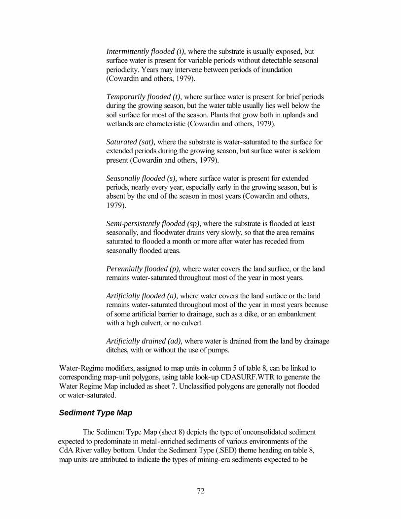
Intermittently flooded (i), where the substrate is usually exposed, but surface water is present for variable periods without detectable seasonal periodicity. Years may intervene between periods of inundation (Cowardin and others, 1979). Seasonally flooded (s), where surface water is present for extended periods, nearly every year, especially early in the growing season, but is absent by the end of the season in most years (Cowardin and others, 1979). Semi-persistently flooded (sp), where the substrate is flooded at least seasonally, and floodwater drains very slowly, so that the area remains saturated to flooded a month or more after water has receded from seasonally flooded areas. Perennially flooded (p), where water covers the land surface, or the land remains water-saturated throughout most of the year in most years.
The term “permanently flooded,” as defined by Cowardin and others (1979) was avoided, because water levels in many parts of the CdA River valley are presently regulated by artificial devices that are not historically permanent. For example, some areas that are now perennially flooded were intermittently to seasonally flooded before present water barriers were built. Conversely, many areas that are presently drained by ditches and pumps would be semi-persistently to perennially flooded without them. Category 6 designates wetland Subclass, which indicates Lacustrine areas with abundant submergent or non-persistent vegetation.
Category 7 designates the wetland plants that are dominant in some Palustrine areas. Wetland plants are identified by abbreviations for their common names, for example common reed (cr), the scientific name of which is Phragmites. Category 8 includes Modifiers, which are numeric or alphabetic post-scripts that are attached to some map-unit names to indicate subtypes or modified types. For example, alluvial terraces at different elevations are numbered topographically, from low to high, as are dredge spoils and dredge-spoil dikes. Outer margins of some sand splays and (or) levee sand deposits are indicated by the post-script (o) for “outer.” Distributaries, now blocked and inactive, are indicated by the post-script (b) for “blocked.” Agricultural lands that are artificially drained and (or) cultivated are indicated by the post-scripts (d) for “drained,” and (f) for “farmed.”
32
Description of Map Units It is conventional to describe geologic map units in order of decreasing age,
thereby developing a geological history. For that reason, map units of the Highland System, which range in age from Precambrian to Holocene, are described first, in order of decreasing age. However, most surficial features of other Systems are Holocene in age. Furthermore, since the floodplain is a predominantly depositional environment from Cataldo Flats to CdA Lake, most sediment now exposed at the surface was deposited during the mining era. Therefore, map units of the river channel and its floodplain are described from upstream to downstream. Descriptions of map units of the Upper Perennial Subsystem are followed by descriptions of map units of the Lower Perennial Subsystem. Man-made features of the Artificial System are described last.
Highland System The Highland System includes map units that represent the geology of hills and valleys that rise significantly above the CdA River floodplain. Highlands are mostly peripheral to the floodplain, but some are within it, and rise above it like islands. Most Highland map-unit boundaries are from a geologic map of the Spokane 1o x 2o quadrangle by Griggs (1973). We added some surficial features near the margins of the floodplain, as noted below. Highland map units of pre-Quaternary age represent bedrock, which commonly is covered by up to 6 m (20 ft) of bedrock-derived colluvium and soil (not indicated on the map). Highland map units of Quaternary age represent unconsolidated surficial sediments, such as landslide and mudflow deposits, and alluvium. Highland map-unit descriptions follow.
HYms Precambrian Y (Middle Proterozoic) Metasedimentary rocks -- Metasedimentary bedrock of the Belt Supergroup, of Precambrian Y (Middle Proterozoic) age. Mostly dark gray argillite (commonly pyritic) and subordinate quartzite of the Prichard and Burke Formations (Griggs, 1973). Includes bedrock outcrops and bedrock-derived surficial colluvium, up to about 6 m (20 ft) thick
HMbv Miocene Basaltic Volcanic rocks -- Basaltic volcanic rocks of the
Columbia River Basalt Group, of Miocene age (Griggs, 1973). Includes basalt and subordinate interlayered sedimentary strata (which are clayey to sandy), and bedrock-derived surficial colluvium and soil, up to about 6 m (20 ft) thick
HMs Miocene Sedimentary rocks -- Semi-lithified clastic sediments of
Miocene age. Areas mapped as HMs are from Griggs (1973), who did not distinguish between semi-consolidated sediments of Miocene and (or) Quaternary age on his 1:250,000-scale map. We interpret such sediments along the CdA River valley to be of Miocene age, and suggest that they were deposited in an ancestral CdA River valley. Relatively wide, straight parts of the present valley follow the Miocene valley, but relatively narrow, sinuous parts of the present valley diverge from the paleo-valley, as marked by erosional remnants of Miocene sediments (sheets 1 and 2).
In a clay pit near Lane, Idaho, we found fossilized leaves of
Miocene age (identified by W. Rember , pers. commun., 1995). Southwest of the clay beds, Miocene basalts fill the trace of the Miocene valley (sheet 2). The clay probably was deposited in a lake that formed behind basalt flows, which dammed the Miocene valley near the present locations of Cave and Black Lakes. Northeast of (and up-valley from) the clay beds, most exposures of the Miocene sediments consist of moderately dipping layers of soft, clayey sandstone, which is exposed in road cuts between
35
Rose Lake and the southwest end of Cataldo Flats, and also between Cataldo and Kingston (sheet 1). We interpret these as erosional remnants of alluvial and (or) lacustrine sediments, deposited in the ancestral CdA River valley during Miocene time. The sediments have since undergone partial lithification, tilting, and erosion.
HQpl Quaternary (Pleistocene) Palouse Loess -- Surficial deposits of
unconsolidated, silty loess (Griggs, 1973), transported and deposited by wind, probably during Pleistocene interglacial ages (Alt and Hyndman, 1995). Loess dunes are common on the tops of basaltic plateaus, which rim the southwestern part of the CdA River valley. The loess represents a potential source of clean sediments for natural and (or) artificial remediation and restoration of the CdA River valley, but much of it now supports agricultural land use.
HQls Quaternary (Holocene) Landslide Debris -- Surficial deposits of
unconsolidated, unsorted debris. Lobate land forms with uneven surfaces on the lower slopes of hillsides are interpreted as deposits of landslide debris. Some landslide deposits are from the 1973 map by Griggs, but others were identified during this project by stereoscopic inspection of aerial photographs.
HUQmf Quaternary (Holocene) Mudflow Deposit –- Surficial deposit of
unconsolidated fine-grained sediments, in a lobate land form, which extends across the transition from Highland to Upland, at the toe of a landslide, south of the river, near Dudley (sheet 1). The lobate topographic expression and the low gradient across which the deposit extends, indicate that it formed as a flowing mass that was more fluid than the landslide deposit up-slope from it.
HQta Quaternary (Holocene to Present) Alluvium of tributary streams --
Surficial deposits of unconsolidated alluvium (mostly gravel and sand) HUif Highland-Upland (Present) intermittently flooded –- Areas that are
transitional from Highland to Upland, and are intermittently flooded. These generally are on the outer margins of the floodplain.
36
Upper Perennial Subsystem
The CdA River upstream from Cataldo Flats is assigned to the Upper Perennial Subsystem of Cowardin and others (1979), because its gradient is sufficiently steep, and its currents sufficiently swift to winnow silt and sand from its cobble-gravel bottom surface. From the confluence of the North and South Forks to the town of Cataldo, the perennially active channel-way of the river is composite and braided. Upstream from Cataldo Flats, the active channel-way is bounded by erosional remnants of alluvial terraces, which form up to four progressively higher benches above the perennially active channel-way. All four alluvial terraces are within the floodplain, but the lower terraces are flooded more frequently than the upper ones, and therefore they receive more metal-enriched sediment. High-water over-flow channels and partly-filled channel scars braid across some of the alluvial terraces, leading to marshes and oxbow ponds, which slowly drain back to the river. Metal-enriched sediments, which are present on most of the terraces, are thickest in high-water (overflow) channels and partly filled channel scars that braid across them (figure 7). Map-unit descriptions follow.
Uat2
Uat3
Uat1
Rg
Rgb
Hms
Uat2
Figure 7. Schematic block diagram, showing features typical of the braided, gravel-bottomed CdA River and alluvial terraces of its floodplain, between the confluence and Cataldo Landing (modified from Williams and Rust, 1969). The alluvial terraces are in the active floodplain, and are blanketed by metal-enriched sediment. On steep faces, thickness of the layer of metal-enriched sediment is represented in dark gray.
Channel ScarsUcs Channel scar (partly filled trace of an abandoned river or overflow channel)Ucsl Channel-scar levee (natural levee adjacent to a channel scar)
Natural LeveesUls Levee sand (sand wash-over deposit on a natural levee)
Palustrine Features
PEcr Marshy area with Emergent vegetation (common reed)PEs Marsh with Emergent vegetation, seasonally floodedPEp Marsh with Emergent vegetation, perennially saturated to floodedPA Marsh with > 30% of Aquatic vegetationPOw Small pond with Open water
3 8
39
Riverine Features, Upper Perennial Subsystem
Rpm Pre-mining-era sediments – Sediments that underlie metal-enriched sediments, and that were deposited before the metal-enriched sediments that overlie them. Pre-mining-era sediments of the CdA River valley below the confluence of the North and South Forks probably were deposited before the bank-full episode of 1890, four years after start-up of the Bunker Hill mill. Pre-mining sediments are not exposed at the surface upstream from Cataldo Flats, and are not shown on sheet1. However, they are shown diagrammatically on the block diagram in figure 7. As indicated in figure 7, metal-enriched sediments are underlain by pre-mining-era gravel, and the gravel is underlain by lacustrine clayey silt deposited in Glacial Lake Coeur d’Alene. At the lower end of Smelterville Flats, about 1 m (3.3 ft) of metal-enriched sediment overlies about 15 m (50 ft) of pre-mining-era gravel. This upper gravel overlies about 15 m (50 ft) of lacustrine clayey silt (deposited in Glacial Lake CdA). The lacustrine beds overlie about 9 m (30 ft) of basal gravel. Bedrock is at 40 m (130 ft) below the surface (Dames and Moore, 1990). A similar but down-valley thickening sequence of stratigraphic units is expected from the confluence to Cataldo Flats. Norbeck (1974) estimated maximum depth to bedrock as 60 m (196 ft) near Cataldo, on the basis of a seismic refraction traverse across the floodplain of the CdA River between Cataldo and Skeel Gulches.
Rg Gravel-bottomed channel -- Channel with a bottom of unconsolidated
cobble-gravel. Cobbles are abundant at the surface, where finer particles are winnowed away by flowing water. However, finer-grained particles (pebbles, granules, sand and silt grains), entrained in gravel deposited during waning stages of high-flow episodes, are present between cobbles beneath the surface. In metal-enriched gravels, most of the metals probably are contained in relatively fine-grained interstitial particles, and (or) in particle coatings of iron- and (or) manganese-oxides.
Rgb Gravel bar -- Accumulation of gravel, deposited along a river or stream,
where a decrease in current velocity induces deposition (after Bates and Jackson, 1987). Gravel bars are common in the braided reach of the Upper Perennial Subsystem of the CdA River, from the confluence of the North and South Forks, to the meander bend at Skeel Gulch, south of Cataldo and east of Cataldo Mission (sheet 1 and figure 3).
Rhc High-water channel (active during floods) –- High-water channel that is
active during high-water episodes, and is therefore considered intermittently Riverine, even though it carries floodwater onto the floodplain. High-water channels diverge from the channel-way at low
40
places in the riverbanks. Between Enaville and Cataldo Mission, high-water channels commonly meander and braid across alluvial terraces adjacent to the active channel-way of the CdA River (sheet 1). During high-water episodes, floodwater enters high-water channels, flows down-valley, and collects in marshes that drain back into the river, down-valley. High-water channels generally are partly filled with metal-enriched sand and silt.
Upland Features of the Terraced Floodplain
Uat Alluvial terrace –- Stream terrace, composed of unconsolidated alluvium, including gravel, forming a long, narrow, relatively level or gently inclined surface, bounded on one side by a steeper descending slope, and on the other by a steeper ascending slope (Jackson and Bates, 1987). Erosional remnants of four alluvial terraces are present along the North Fork and main stem of the CdA River, upstream from Cataldo Mission (sheet 1). Terrace levels are numbered upward from the lowest and youngest terrace level above the braided channel-way, to the highest and oldest terrace level, as follows:
Alluvial terraces are produced by renewed down-cutting of the floodplain or valley floor by a rejuvenated stream (Jackson and Bates, 1987). Stream rejuvenation commonly occurs in response to a lowering of the local base-level of erosion. Glacial Lake Coeur d’Alene once extended up the CdA River valley to near the present site of Kellogg (Molenaar, 1988). As its dam of unconsolidated sediment eroded, the shoreline of the Glacial Lake moved down-valley, and gravel deposition advanced down-valley, covering lakebed sediments from Kellogg to Cataldo Mission. As the lake level dropped, the lakeshore retreated toward its present position at Harrison, and the local erosional baseline was lowered. Upstream from Catlado Landing the river responded by eroding down into previously deposited gravels. Erosional remnants of former valley bottoms now form terraces along the valley margins. The terraces are all post-glacial (Holocene) in age, or less than 10,000 years old. The highest terrace (Uat4) is the oldest, and the lowest (Uat1) is the youngest. Upstream from Kingston, the uppermost alluvial terrace (Uat4) slopes gently toward the river and down-valley. Its uppermost part was just above the high-water line of the 1996 winter flood. In general, the higher terraces are flooded less frequently than the lower terraces, and therefore have received less metal-enriched sediment. From Kingston to Cataldo Landing, alluvial
41
terraces tend to slope gently down-valley and away from the tops of natural levees along their riverside margins. The three alluvial terraces between Cataldo and Cataldo Landing are laced with braided high-water channels and channel scars (figure 7).
Ucs Channel scar -- Trace of an abandoned alluvial channel, marked by an
elongate, commonly curved, meandering and (or) braided topographic depression, more-or-less filled by sandy to silty alluvial sediments. Floodwater and suspended sediments collect along braided high-water channels and channel scars. Channel scars are particularly abundant on Cataldo Terraces, Mission Terraces, and Latour Terraces (figure 3). In addition to the mapped channel scars, these areas bear a multitude of discontinuous scars of multiple generations of braided channels, and crescentic segments of meander-bend cut-banks. Along channel scars that have been active during the mining era, accumulations of metal-enriched sand and silt locally are more than 2 m (7 ft) thick. Braided networks of channel scars commonly lead to down-valley lateral marshes, which drain back to the river.
Ucsl Channel-scar levee -- Natural levee along the margin of a channel scar
(Ucs). Channel-scar levees form by over-bank deposition of sediments, along the margins of channel scar. Natural levees of abandoned channels form embankments of oxbow ponds north of Cataldo Mission (sheet 1).
Uls Levee sand –- Sand deposits on a natural levee. Natural levees are built up
by deposition of relatively coarse sediments near the river, as floodwater washes over the normal riverbanks, and its velocity, turbulence, and carrying capacity decrease (Bates and Jackson, 1987). The levee sand deposit on alluvial terrace 3 (Uat3), north of Cataldo, formed during the 1933 flood, before the present artificial levee was built. Levee sands down-valley from Cataldo are light-tan sand deposits along the river margins, which are relatively non-vegetated, because vegetation is frequently smothered by added layers of sand.
Palustrine Habitats of the Terraced Floodplain PEcr Palustrine with Emergent common reed – Marshy area with common reed
(Phragmites) as the predominant vegetation. Common reed was planted on dredge spoils at Cataldo Flats to control wind-blown sand and dust. It has thrived where the water table is at or near the surface. It has now spread to other wet and semi-wet, sandy areas, where it tends to produce almost impenetrable growths of tall reeds.
PEs Palustrine with Emergent vegetation, seasonally flooded –- Marshy to
boggy area, flooded in the spring season with standing water, which drains
42
during the summer, leaving the ground more-or-less saturated (water-logged), so that Emergent hydrophytic vegetation is predominant
PEp Palustrine with Emergent vegetation, perennially flooded -- Marsh that has
standing water continuously through the growing season, is saturated in autumn, and has Emergent vegetation
PA Palustrine with Aquatic vegetation –- Pond with more than 30 percent of
Aquatic vegetation at the surface (as estimated from aerial photographs taken during the growing season)
POw Palustrine with Open-water –- Pond, slough or fen with open water.
Oxbow ponds north of Cataldo Mission occupy arcuate channel scars.
Lower Perennial Subsystem The CdA River down-stream from Cataldo Landing is assigned to the Lower Perennial Subsystem of Cowardin and others (1979), because it has a low gradient, slow to negligible flow during ordinary conditions, and a sandy to muddy bottom. At Cataldo Landing, where the water-surface gradient approaches zero during the summer months, the river current slackens, and a large central bar of metal-enriched sand nearly fills the wide channel. From there to CdA Lake, the meandering river channel contains thick deposits of metal-enriched sand (figure 8). The river channel commonly is bounded by steep banks, cut in bank-wedge deposits of red, metal-enriched sand and silt, previously deposited on the riverside margins of natural, pre-mining-era levees of gray silty mud.
Over-bank deposits of metal-enriched sand extend over the tops of natural levees, generally fining and thinning from the levee tops toward lateral flood basins (figure 8). In Upland environments of natural levees, which are only flooded intermittently, metal-enriched sand and silt become iron stained as iron-bearing minerals undergo oxidative weathering. In water-saturated, vegetation-rich Palustrine and Lacustrine environments of lateral marshes and lakes, metal-enriched silt and mud generally are dark gray to black, indicating transitional to reducing conditions. Sand splays extend through low passes in levees, and fan out onto the floodplain. Distributary streams and man-made canals transport metal-enriched sediments across the floodplain, onto their natural levees, and into lateral marshes and lakes (figure 8). Map-unit descriptions follow.
PEs�
UlbUls
Ucs
RsLlt
Ulb
RpmUls Rbw
Uss
Udis
RsUms
Uls
Channel
Levee
Lateral Lake
Lateral Marsh
FLOOD BASINFLOOD BASIN
FLOODPLAINMEANDER-BELT RIDGE
DistributaryStream
Levee
Sand Splay
Meander Scroll Set
Point Bar
Bank Wedge
Pre-mining-era Sediments
Pre-mining-eraPoint Bars
Figure 8. Schematic block diagram, showing features typical of the meandering, sand-bottomed CdA River and its floodplain, between Cataldo Landing and Harrison (modified from Reineck and Singh, 1980; Collison, 1978; and Leopold, 1997). Dotted arrows represent flow paths. On steep faces, thickness of the layer of metal-enriched sediment is represented in dark gray.
Riverchute present
pre-miningbottom
bottom
Summer water level
Back-slope
Natural Levee
Sand
Metal-enriched sand and silt
Metal-enric
hed
silt and m
ud
43
Table 4. Map Units of Lower Perennial Riverine, Trans-Floodplain, and Upland Features
map-unit label Map Unit Classification, Definition
Lower Perennial Riverine FeaturesRiver Channel
Rpm Pre-mining-era sedimentsRscb Central sand bar Rs Sand-bottomed channel (includes lateral bars, bottom-fill, point bars)Rsb Sand-bar beach (subaerial at summer water level)Rbw Bank wedge of metal-enriched sediments (wedge thins from riverbank to levee top)
Linear Featuresgreen Stream, intermittentblue Stream, perennial" " " River cutbank, high ' ' ' River cutbank, low
Trans-Floodplain FeaturesDistributary Sreams and their Natural Levees
Rdisc Distributary stream with wide, Riverine channelUdis Distributary, including channel and Upland natural-levees Udisb Distributary, with blocked channel and Upland natural-leveesPdisE Distributary, including channel and Palustrine natural levees with Emergent vegetationPdisbE Distributary, with blocked channel and Pallustrine natural levees with Emergent vegetation
Ucs Channel scar (trace of semi-abandoned to abandoned channel, chute, or meander) Natural Levees and Meander Scrolls
Ucsl Channel scar levee(s)Uls Levee sand (sparsely vegetated)Ulso Levee sand, outer margin (siltier, more vegetated than Uls)Ulb Levee back-slope (siltier, more vegetated than Uls or Ulso)Ulbf Levee back-slope, farmed (plowed)Ums Meander-scroll set Umsf Meander-scroll set, farmed
Sand SplaysUss Sand splay or crevasse splay (sparsely vegetated)Ussc Sand-splay channel (crevasse) Usso Sand splay, outer margin (siltier, more vegetated than Uss)
44
45
Riverine Features, Lower Perennial Subsystem
Rpm Pre-mining-era sediments –- Sediments deposited before mining began in the CdA River drainage basin. Pre-mining-era sediments underlie the entire CdA River channel and its floodplain, but they are exposed (and therefore mapped) only along non-depositional side-slopes of the river. Exposures of pre-mining sediments along the river side-slopes commonly are so narrow that their width had to be somewhat exaggerated in order for them to be portrayed on sheets 1 and 2. Pre-mining-era sediments, exposed on channel side-slopes and lower banks, consist mostly of slippery gray silty clay. However, pre-mining-era river-bottom sediments consist mostly of sand, as indicated by drilling, and pre-mining-era sediments in lateral marshes and lakes consist mostly of organic peat, as indicated by pits and drill cores.
Pre-mining-era sediments directly below metal-rich mining-era sediments commonly contain as much as 500 ppm of lead and 1,000 ppm zinc. However, lead concentrations in pre-mining-era sediments generally decrease downward, to between 50 and 25 ppm or less by about 20 cm below the basal mining-era sediments. Zinc concentrations also decrease downward to between 100 and 75 ppm or less by about 40 cm below the basal mining-era sediments (A.A. Bookstrom and S.E. Box, unpub. data, 1993 to 1998). We interpret this to indicate that metals leached from mining-era sediments are chemically transported downward and deposited in underlying pre-mining-era sediments. More zinc than lead is leached, and zinc is transported farther down-section than lead, because zinc is more geochemically mobile than lead. We therefore suggest that primary concentrations of lead and zinc in pre-mining-era sediments of the CdA River valley are similar to mean concentrations of lead (22 ppm) and zinc (76 ppm) in sediments in the St. Joe River valley, where no significant mining has occurred (Abraham, 1994).
Rscb Central sand bar -- Sand bar in the center of the river channel. A large
central sand bar nearly fills the wide meander bend at Cataldo Landing, where the river gradient flattens, and the summer water-surface gradient approaches nil. This central sand bar is at the transition from the gravel bottom of the Upper Perennial Subsystem to the sand bottom of the Lower Perennial Subsystem. Grain size of sediments on the central sand bar generally decreases downstream. Coarse sand, with sparse pebbles, grades to coarse- to medium-grained sand at the downstream end of the bar. The central sand bar at Cataldo Landing is interpreted as a friction-dominated middle ground bar, as described by Wright (1977) and Elliott (1986).
46
Rs Sand-bottomed river channel -- Sand-covered part of river bottom, including sand-dominated bottom-fill, point bars, and lateral bars. Metal-enriched sand covers most of the trough of the pre-mining-era riverbed west of Cataldo Landing, as indicated by drilling, sonar, and ground-penetrating radar transects (S.E. Box and A.A. Bookstrom, unpub. data, 1994 to 1997; USEPA, 1998).
Along relatively straight stretches of the river channel, the trough of the pre-mining-era channel is partly filled with metal-enriched sediments, which form a relatively flat, sandy bottom, bounded by sloping sides of relatively fine-grained, and cohesive pre-mining-era sediments (figure 8 and sheets 1 and 2). Sand waves with amplitudes of about 1 m (3.3 ft) are common along straight, sand-bottomed stretches of the river from Frutchey’s Meadow to Rose Lake (as indicated by longitudinal sonar depth profiles). Sand waves probably result from hydraulically rough flow (Gordon, McMahon and Finlayson, 1992), which can occur during floods, especially winter floods.
Point-bar deposits of metal-enriched sand are present the inside margins of meander bends (figure 8 and sheets1 and 2). Point-bar deposits generally thicken from the levee top toward the deep axis of the channel, which is partly filled with sandy metal-enriched sediments (S.E. Box and A.A. Bookstrom, unpub. data, 1994-1996; USEPA, 1998).
Lateral bars of metal-enriched sand line both sides of the river, just upstream from the central sand bar at Cataldo Landing (sheet 1). Lateral bars also are present on the inside margins of incipient meanders, and they extend down-stream from many point bars (sheets 1 and 2).
Average thickness of sandy metal-enriched sediments in the river channel decreases down-river, from 3.5 m between Cataldo Landing and Rose Lake, to 2.7 m from there to Medicine Lake, and 2.2 m from there to Harrison, as calculated from drilling and ground-penetrating radar traverses (A.A. Bookstrom and S.E. Box, unpub. data, 1996; and USEPA, 1998). Metal-enriched sand deposits in the river channel generally coarsen upward, from basal very fine-grained sand with > 10,000 ppm of lead, to medium-grained sand with between 6,000 and 1,000 ppm of lead at the top (S.E. Box and A.A. Bookstrom, unpub. data, 1995 to 1997).
Rsb Sand bar beach –- Upper part of a sand bar, consisting of metal-enriched
sand, which is subaerial at summer water level. Relatively large sand bar beaches that are accessible to the public are identified on the map, because they are popular recreation areas.
Rbw Bank wedge of metal-enriched sediments -- Wedge-shaped deposits of
metal-enriched sediment. Bank-wedge deposits extend from riverbanks to the levee tops, along riverside margins of the natural levees, (figure 8 and sheets 1 and 2). Bank thickness of metal-enriched sediments commonly ranges from about 2 to 0.4 m (6.6 to 1.3 ft), whereas levee-top thickness of metal-enriched sediments commonly ranges from about 1.4 to 0.3 m (4.6
47
to 1 ft). Thus, ratios of bank- to levee-top thickness of bank wedge deposits commonly range from about 0.7 to 0.75. In the upper valley, banks and levee tops are relatively high, levee tops are close to the riverside, and bank-wedge tops and bottoms obviously converge toward the levee top. In the lower valley, banks and levee tops are relatively low, levee tops are set back from the riverside, and bank-wedge tops and bottoms converge gradually toward the levee top.
Bank-wedge sediments generally consist of layers and lenses of cross-bedded, metal-enriched sand and silt, which are oxidized and cemented by reddish brown, orange, yellow and black oxides and oxy-hydrides of iron and manganese. These colorful, oxide-cemented sand and silt deposits generally overlie gray silty mud of the pre-mining-era river-channel side-slope and (or) natural levee. Where the thick riverside margin of the bank wedge deposit has not been much eroded, the contact between it and underlying pre-mining-era sediments is commonly at about summer water level. However, on outside (cut-bank) margins of meander bends, the bank wedge commonly is eroded back toward the levee top, so that only its thin edge is preserved, and beneath it the cut-bank exposes gray, silty mud of the pre-mining-era levee.
Bank-wedge deposits of metal-enriched sediments probably formed mostly before 1968, when the river consistently carried abundant suspended tailings. Since then, bank-wedge deposits have undergone lateral erosion, even as they have continued to thicken vertically, with the average addition of 8 cm of metal-enriched sediments since deposition of the 1980 volcanic-ash marker bed. Evidence of lateral erosion of bank-wedge deposits includes bank-liner posts, which now stand well out into the river, and relatively flat benches, which are present at about summer water level, especially along straight stretches of the river. These benches indicate that the steep face of the bank-wedge has eroded and retreated farther than the underlying channel side slopes. Such bank-wedge retreat probably is the result of erosion, resulting from a combination of groundwater drainage from the banks to the river, wave action from wind and powerboat wakes, and river currents during floods (especially winter floods).
Linear Riverine features are too narrow to be represented as polygons at the map
scale, but are shown by decorated or colored lines on sheets 1 and 2.
Stream, intermittent -- Narrow stream that carries water intermittently
Stream, perennial -- Narrow stream that carries water perennially. River cutbank, high -- Steep, relatively non-vegetated bank, more than about 1 m (3.3 ft) high (common up-river from Swan Lake)
48
River cutbank, low -- Steep, relatively non-vegetated bank, less than about 1 m (3.3 ft) high (common down-river from Swan Lake)
Trans-Floodplain Features
Distributary Streams and their Natural Levees
Rdisc Distributary stream (wide) –- Channel that diverges from the main river channel without returning to it. A distributary channel is mapped and labeled Rdisc if it is wide enough to be represented by a polygon at the map scale, but is mapped as a linear intermittent stream where it is too narrow to be represented by a polygon. Although wide distributary stream channels are classified as Riverine, they are grouped here with distributary stream deposits, which are classified as Upland features, because their natural levees stand somewhat above the river and its lateral flood basins.
Udis Distributary stream deposits –- Distributary stream, including its natural
levees. Distributary streams diverge from the river, and do not return to it (Bates and Jackson, 1987). Distributary streams connect the river to lateral lakes and marshes of its floodplain. At flood stage, they transport river water and suspended metal-enriched sediments from the river to their levees and to lateral marshes and lakes of the flood basins. During episodes of decreasing water levels, distributary streams return water from the flood basins to the river.
Udisb Distributary stream (blocked) –- Distributary stream, the channel of which
is blocked, so that it has become disconnected from the river and is relatively inactive. One example is the distributary at Rose Lake, which is blocked by a road embankment, which has no culvert or bridge to allow passage of water from the river to the distributary stream.
PdisE Distributary stream, and levees with Emergent vegetation –- Marshy part
of a distributary, with Emergent vegetation on its levees. Distributary streams diverge from the river and connect it to lateral marshes and (or) lakes
PdisbE Distributary stream (blocked), and levees with Emergent vegetation --
Marshy part of a blocked distributary stream, with Emergent vegetation on its levees
49
Upland Features of the Floodplain The Upland System, in the Lower Perennial Subsystem, includes parts of the floodplain that are mostly subaerial, but are flooded intermittently, when the river overflows. The Upland System includes features that comprise the river’s natural levees, which form its meander-belt ridge, as illustrated in figure 8. Along straight segments of the river channel, floodwaters overflow both banks more-or-less evenly, depositing over-bank sediment on both sides of the river, to build similar natural levees on both sides of the river. On outside margins of meanders, river currents accelerate and spiral downward, eroding cut-banks, and overflowing tangentially, to form levee sand deposits (figure 8). On inside margins of meanders, river currents slacken and spiral upward, depositing sediments to form point-bar deposits (figure 8). Thus, the river channel migrates laterally and down-valley, by eroding its floodplain along outside margins of its meanders, while adding successive point bar deposits to inner margins of its meanders. Curved crests of successive pre-mining-era point-bar deposits, with troughs between them, form meander scroll sets, which are blanketed by overlying metal-enriched sediments (figure 8). Distributary streams, with natural levees, diverge from the river, connecting it to lateral marshes and lakes. Sand splays fan-out onto the floodplain from low passes or wide crevasses in its natural levees, through which floodwater flows from the river onto the unconfined floodplain (figure 8). Upland-System map units of the Lower Perennial Subsystem are explained below.
Erosional Remnants UerMc Erosional remnant of Miocene clay –- Erosional remnant of Miocene clay
in an Upland part of the floodplain (near Medicine Lake)
Channel Scars
Ucs Channel scar -- Trace of an abandoned alluvial channel, such as a meander bend, high-water channel, or chute cutoff, marked by an elongate, commonly curved, topographic depression, more-or-less filled with sandy to silty alluvial sediments. Metal-enriched alluvium, which blankets the floodplain, generally thickens within channel scars.
Multiple channel scars on Latour Terraces, south of Cataldo Landing, indicate partly-filled remnants of abandoned river channels (sheet 1 and figure 3). As they fill, these abandoned river channels evolve into high-water channels, and then into channel scars.
A channel scar south of Highway 3 and west of Rose Lake is an example of a chute cutoff (sheet 1). A chute cutoff is a channel scar that “short cuts” across the inside of a meander bend (figure 8), as river flow (or overflow) is diverted along a trough between crests of adjacent point-bar deposits of a meander scroll set (Bates and Jackson, 1987).
50
Levees and Meander Scrolls Ucsl Channel-scar levee -- Natural levee along the margin of a channel scar
(Ucs). Channel-scar levee(s) form by over-bank deposition of sediments along the margin of an alluvial channel, as it evolves from an active channel to a relatively abandoned and inactive channel scar.
Uls Levee sand –- Sand wash-over deposits on a natural levee. Natural levees
are built up by deposition of successive wash-over deposits, which form by deposition of relatively coarse sediments near the river, as it washes over its normal banks, and its velocity, turbulence, and carrying capacity decrease (after Bates and Jackson, 1987). Aerial photographs show levee sand deposits as very light-tan colored, relatively non-vegetated areas along the river margins. Along relatively straight segments of the river channel, levee sand deposits form symmetrically, along both sides of the river. Along outside and lower outside margins of meander bends, levee sands are particularly well developed, as a result of centrifugal and down-valley overflow (sheet 1).
Within the levee sand deposits, relatively thick layers of sand, deposited during high-flood stages, commonly are interlayered with thin, silty layers, deposited during waning flood stages. Grass duff horizons within the sand section indicate that many generations of grass have been covered by layers of sand, added by a succession of floods. In 1993, an average of 8 cm of metal-enriched sand, containing 2,000 to 6,000 ppm of lead, had been added to Uls deposits since deposition of the 1980 volcanic-ash marker bed (S.E. Box and A.A. Bookstrom, unpub. data, 1993). More sand has been added by a continuing succession of floods, the largest of which occurred in February, 1996.
Ulso Levee sand (outer margin) –- Outer margin of a levee sand deposit, which
aerial photos show to be relatively well vegetated. The outer margin is lower, thinner and finer grained than the main body of the levee sand deposit. The presence of vegetation can be interpreted to indicate longer intervals between coverings of vegetation by sand deposition, or it can be interpreted to result from wetter conditions, more favorable to plant growth.
Ulb Levee back-slope –- Slope on the back side of the levee, inclined gently
away from the river and its levee crest, and toward lateral flood basins of the surrounding floodplain (after Bates and Jackson, 1987). Deposits of levee sand commonly cover the upper part of the levee back-slope. Peripheral to the levee sand deposits, the levee back-slope tends to be covered by a relatively thin veneer of silty, reddish metal-enriched sediments, which locally have higher metal contents than the coarser-
51
grained levee sands (A.A. Bookstrom and S.E. Box, unpub. data, 1993 to 1998). Grasses and other terrestrial vegetation, including deciduous and conifer trees are common on the upper parts of levee back-slopes. Scrub-shrub vegetation commonly is present along the boundary between well-drained levee back-slopes, and water-saturated Palustrine environments.
Ulbf Levee back-slope, farmed -- Levee back-slope that has been or is being
farmed. In farmed areas, metal-enriched sediments commonly are plowed under, broken, and mixed with pre-mining-era soils.
Ums Meander-scoll set -- Set of long, parallel, closely spaced, arcuate ridges
and troughs formed along the inner bank of a meander bend, as the channel migrates laterally down-valley and toward the outer bank (after Bates and Jackson, 1987). Meanders migrate down-valley and increase in amplitude by erosion of their outside-downstream margins, combined with formation of point-bar deposits along their inside-downstream margins. The curved ridges of a meander scroll set indicate positions of the crest-lines (or point-bar levees) of successive point-bar deposits. Although presently active point bars consist entirely of metal-enriched sediments, pre-mining-era meander-scroll sets consist of uncontaminated sediments, blanketed by a surficial veneer of metal-enriched sediments (figure 8).
Umsf Meander-scar set, farmed -- Area of a meander-scar set that is farmed and
has been plowed, so that the surficial veneer of metal-enriched sediment may be turned under, broken-up, and mixed with uncontaminated pre-mining-era sediment
Sand Splays Uss Sand splay –- A small alluvial fan or other outspread deposit formed
where an overloaded stream breaks through a levee, spreads onto the unconfined floodplain, looses velocity, and deposits sand (after Bates and Jackson, 1987). Synonyms are floodplain splay, crevasse splay, channel splay, and (or) sand breakout. A plume-shaped sand splay forms where a relatively narrow, single channel breaches the levee, as at Frutchie’s meadow, between Cataldo Flats and Dudley (sheet 1). A fan-shaped sand splay forms where a wide channel breaches the levee, and bifurcates away from the river, as at Strobl Marsh, near Killarney Lake (sheet 1). Sand-splay deposits generally are thickest and coarsest-grained near the river, and thinner and finer-grained towards their outer edges.
Two large sand splays are present in a wide section of the CdA
River valley, between Rose Lake and Killarney Lake. During major floods, the level of CdA Lake rises, and water backs into that area from CdA Lake. The back-flooded area is therefore regarded as a flood-stage
52
delta plain, where relatively fast-flowing riverine floodwater enters relatively slack water backed-up from CdA Lake.
Ussc Sand-splay channel -- Channel that carries water and suspended sediments
from the river to a sand-splay deposit. Sand-splay channels bifurcate away from the river, distributing water and sand onto the floodplain, to form a fan-shaped sand splay deposit
Usso Sand splay (outer margin) – Outer margin of a sand splay deposit, which is
more vegetated than the central part of the deposit. The outer margin is lower, thinner and wetter than the central part. The presence of vegetation can be interpreted to indicate longer intervals between smothering of vegetation by sand deposition, or it can be interpreted to result from wetter conditions, more favorable to plant growth.
Palustrine Habitats of Lateral Flood Basins Palustrine habitats include vegetated wetlands traditionally named swamp (wooded wetland), meadow (low-lying sedge- or grassland), bog (spongy ground with sedges or peat moss), marsh (soft wetland with Emergent vegetation), slough (muddy place, sluggish channel, or small pond), or fen (low land covered with water). These terms are from Cowardin and others (1987), and their parenthesized descriptions are from Bates and Jackson (1987). Palustrine habitats of lateral flood basins of the CdA River valley include meadows, marshes and sloughs, into which metal-enriched sediments are deposited from suspension in floodwaters. In general, metal-enriched sediments of lateral marshes are silty to muddy, and organic-rich. They commonly overlie pre-mining-era peat, which is almost wholly organic. Both were deposited and are stored in water-saturated environments, under predominantly reducing conditions. Most lateral marshes have seasonally Palustrine rims, which are flooded during the spring and summer but drained during the fall and early winter. Metal-enriched sediments stored in seasonally Palustrine areas are exposed to alternating wet and dry, reducing and oxidizing conditions. This enhances the geochemical mobility of metals in seasonally Palustrine areas. Palustrine map units are defined and described as follows, and arranged (more-or-less) in order of increasing wetness and (or) water depth. Water depths at summer water level were estimated on the basis of plant types present, and on the basis of depth measurements made by Campbell and others (1999), while collecting geochemical samples of bottom-surface sediments from Palustrine and Lacustrine habitats in the CdA River valley.
Palustrine Habitats with Emergent VegetationPtaE Tributary alluvium in Palustrine habitat with Emergent vegetationPE Palustrine habitat with Emergent vegetationPEsf Emergent vegetation, seasonally flooded, farmedPEsdf Emergent vegetation, seasonally flooded, artificially drained, farmedPEs Emergent vegetation, seasonally floodedPEsT Emergent Terrestrial vegetation (Scrub-shrub, grass), seasonally floodedPEcr Emergent vegetation (common reed predominant)PEspdf Emergent vegetation, semi-persistently saturated, but artificially drained, farmedPEsp Emergent vegetation, semi-persistently saturated to floodedPEp Emergent vegetation, perennially saturated to floodedPEph Emergent vegetation, perennially saturated to flooded (horsetail reed predominant)PEpr Emergent vegetation, perennially saturated to flooded (wild rice predominant)
Palustrine Habitats with Aquatic Vegetation PEphA Emergent > Aquatic vegetation, perennially saturated to flooded (horsetail reed predominant)PEA Emergent and lesser aquatic vegetationPAT Aquatic and Terrestrial (Aquatic peat moss, supporting Terrestrial vegetation) PAE Aquatic and lesser Emergent vegetationPA Aquatic, with > 30% of aquatic vegetation at the surfacePAnp Aquatic, non-persistent vegetation
Palustrine Habitats with Open water POw Open water
53
54
Palustrine Habitats with Emergent Vegetation PtaE Tributary alluvium with Emergent vegetation –- Marshy or swampy
alluvium of a tributary stream, with Emergent vegetation PE Emergent vegetation -- Marsh with Emergent vegetation PEsf Emergent vegetation, seasonally flooded, farmed – Meadow, flooded in
the spring, but naturally drained and farmed in the summer (presently or recently). In such areas, metal-enriched sediments commonly are plowed under, and natural Emergent hydrophytic vegetation is replaced with cultivated terrestrial grasses and grains
PEsdf Emergent vegetation, seasonally flooded, artificially drained and farmed --
Meadow, flooded in the spring, artificially drained by ditches, and farmed. In such areas, metal-enriched sediments commonly are plowed under, and natural Emergent hydrophytic vegetation is replaced with cultivated terrestrial grasses and grains. In some of these areas, pumps are used to move water from collector ditches to the river.
PEs Emergent vegetation, seasonally flooded –- Marshy to boggy area, flooded
in the spring season with standing water, which drains during the summer, leaving the ground more-or-less saturated (water-logged), so that Emergent hydrophytic vegetation is predominant. Hydrophytic vegetation grows in water or in soil that is too waterlogged for most plants to survive (Cowardin and others, 1979).
PEsT Emergent and Terrestrial vegetation, seasonally flooded -- Marshy to
swampy area that is flooded in the spring season, and has both Emergent hydrophytic and Terrestrial vegetation (Grass, Scrub-shrub, or Forest). A narrow rim of scrub-shrub vegetation surrounds many seasonally marshy areas, but has only been mapped where it is sufficiently wide to be resolved at the map scale.
PEcr Emergent vegetation (common reed) – Marshy area where common reed
(Phragmites) is the dominant vegetation. Common reed appears to grow best in sandy areas where the zone of groundwater saturation is at or near the ground surface.
meadow, which remains mostly saturated to inundated well after floods have receded, but is artificially drained and farmed in the summer. In most of these areas, pumps are used to move water from collector ditches to the river. Metal-enriched sediments may be plowed under, and natural
55
Emergent hydrophytic vegetation is partially replaced by cultivated terrestrial grasses and grains.
PEsp Emergent vegetation, semi-persistently flooded -- Marshy meadow with
Emergent hydrophytic vegetation, which is poorly drained, and remains mostly saturated to inundated well after floods have receded. Areas that were mostly inundated one month after the 1996 winter flood, as indicated by a LANDSAT image (USGS, 1996), were mapped as PEsp.
PEp Emergent vegetation, perennially flooded -- Marsh that has standing water
continuously through the growing season, is saturated in autumn, and has Emergent vegetation
PEph Emergent vegetation (horsetails), perennially flooded -- Marsh that has
standing water continuously through the growing season, and has horsetail reed (Equisetum), as the dominant Emergent vegetation
PEpr Emergent vegetation (wild rice), perennially flooded -- Marsh that has
standing water throughout the growing season, and has wild rice (Zizania aquatica L.) as the dominant Emergent vegetation
Palustrine with Aquatic Vegetation PEphA Emergent vegetation (horsetails), and lesser Aquatic vegetation -- Marsh
that has standing water continuously through the summer. Most of the vegetation consists of Emergent horsetail reeds, but Aquatic vegetation is present in relatively small areas of deeper water
PEA Emergent and lesser Aquatic vegetation -- Marsh or slough with Emergent
vegetation and lesser amounts of Aquatic vegetation PAT Aquatic and Terrestrial vegetation –- Bog with Aquatic peat moss
(Sphagnum.) that supports Terrestrial vegetation (Grass, Scrub-shrub or Forest)
PAE Aquatic and lesser Emergent vegetation –- Slough or fen with mostly
Aquatic vegetation and lesser amounts of Emergent vegetation PA Aquatic vegetation –- Slough or fen with more than 30 percent of Aquatic
vegetation at the surface (as estimated from aerial photographs taken during the growing season)
PAnp Aquatic non-persistent vegetation –- Slough or fen with more than 30
percent of Aquatic surface vegetation that is non-persistent (as indicated by aerial photographs taken during and after the growing season)
56
Palustrine Habitat with Open Water POw Open-water –- Slough or fen with open water
Lacustrine Habitats of Lateral Flood Basins The Lacustrine System includes map units that represent lakes, which, according to Cowardin and others (1979), are wetlands and deepwater habitats that:
1) are within topographic depressions or a dammed river channels, 2) have no trees or shrubs, and with less than 30 percent coverage of
persistent emergent vegetation or emergent mosses or lichens, and 3) are larger than 8 ha (20 acres) in area that is at least 2 m (6.6 ft) deep.
The Lacustrine System is divided into the Littoral and Limnetic Subsystems. The Littoral Subsystem extends from the shoreward boundary of the system to a depth of 2 m (6.6 ft) below low water (Cowardin and others, 1979). The Limnetic Subsystem includes all deepwater habitats, deeper than 2m (6.6 ft) below low water level (Cowardin and others, 1979).
On sheets 1 and 2 boundaries between Littoral and Limnetic habitats are placed along the 2 m (6.6 ft) depth contour at summer water level. The 2 m depth contour was estimated on the basis of depth measurements by Campbell and others (1999), Woods and Berenbrock (1994), Northwest Map Service (1991), USEPA (1998), and S.E. Box and A.A. Bookstrom (unpub. data, 1993 to 1998). Summer water level is used as the zero reference depth in this report, because in the CdA River valley, summer water level is more consistent and better known than winter low-water level. Summer water level of the CdA River from Cataldo Landing to CdA Lake is at 2,125 ft elev (USGS Harrison gage). However, summer water levels are higher than 2,125 ft elev in some lateral marshes and lakes, which are artificially blocked from draining freely to the river (by such things as dikes, road embankments, and high, or plugged culverts). Lateral lakes of the CdA River floodplain commonly receive suspended metal-enriched sediments from river floodwater that washes over levees, or is delivered via distributaries and canals that connect the lakes directly to the river or to other lakes or marshes that are connected to the river. Many lateral lakes fill the mouths of tributary valleys, which contribute suspended sediments from non-mining areas to lateral lakes, via tributary-stream inlets at the outer margins of the floodplain.
In deep-water (limnetic) environments, metal-enriched sediments are under transitional to reducing conditions, depending on the amount of decaying vegetation. In shallow-water (littoral) environments, sediments may be exposed to alternating reducing and oxidizing conditions, as summer water level is drawn down as much as 2 m, draining much or all of the summer littoral zone, and exposing at least its shallowest surficial sediments to oxidizing conditions.
LittoralLltA Littoral, Aquatic, with > 30% of aquatic vegetationLltAnp Littoral, Aquatic, non-persistent vegetation LltAsb Littoral, Aquatic, submergent vegetationLltE Littoral, Emergent vegetationLltEnp Littoral, Emergent, non-persistent vegetationLltOw Littoral, Open water
LimneticLlmA Limnetic, Aquatic, with > 30% of aquatic vegetationLlmAnp Limnetic, Aquatic, non-persistent vegetationLlmAsb Limnetic, Aquatic, submergent vegetationLlmOw1 Limnetic, Open-water, <10 m deep
Deltaic Features and Environments
Lateral Lake InletsLisb Inlet sand bar
CdA Lake InletLltl Littoral, levee (submerged)Rmsb River-mouth sand bar (littoral)LlmDOw Limnetic, Delta front, Open water, <10 m deep
CdA Lake LlmOw2 Limnetic, Open-water, >10 m deep
57
58
Map Units of the Lacustrine Littoral Subsystem
Lltl Littoral levee –- Submergent levee in shallow water. Littoral levees are present at the mouth of the CdA River, where it flows into CdA Lake.
LltE Littoral, Emergent -- Shallow lake area with Emergent vegetation LltEnp Littoral, Emergent non-persistent -- Shallow lake area with non-persistent
Emergent vegetation (Non-persistent vegetation is visible at the surface in the summer, but not in the winter.)
LltA Littoral, Aquatic -- Shallow lake area, < 2 m (6.6 ft) deep at summer water
level, with more than 30 percent of Aquatic vegetation LltAnp Littoral, Aquatic nonpersistent -- Shallow lake area with more than 30
percent of Aquatic vegetation that is predominantly non-persistent (Non-persistent vegetation is visible at the surface in the summer but not in the winter.)
LltAsb Littoral, Aquatic submergent -- Shallow lake area with more than 30
percent of under-water Aquatic vegetation LltOw Littoral, Open water -- Shallow lake area with open water
Map Units of the Lacustrine Limnetic Subsystem
LlmA Limnetic, Aquatic -- Deep lake area, > 2 m (6.6 ft) deep at summer water level, with more than 30 percent of Aquatic vegetation
LlmAnp Limnetic, Aquatic non-persistent -- Deep lake area with more than 30
percent of Aquatic vegetation that is predominantly non-persistent (Non-persistent vegetation is visible at the surface in the summer but not in the winter.)
LlmAsb Limnetic, Aquatic submergent -- Deep lake area with more than 30
percent of under-water Aquatic vegetation LlmOw1 Limnetic, Open-water < 10 m deep -- Deep lake area, 2 to 10 m (6.6 to 33
ft) deep, with open water. Maximum water depths measured in limnetic environments, from Cataldo Slough to the delta front, are: Cataldo Slough 2.4 m, Mission Slough 2.1 m, Porter Slough 5.2 m, Rose Lake 6.2 m, Bull Run Lake 3.4 m, Killarney Lake 4.9 m, lacustrine part of Hidden Marsh
59
4.6 m, Medicine Lake 5.5 m, Cave Lake 5.7 m, Swan Lake 6 m, Black Lake 6.3 m, Blue Lake 5.4 m, Thompson Lake 6.3 m, Anderson Lake 4 m, and Harrison Slough 2.5 m (Campbell and others, 1999; Woods and Berenbrock,1994), Northwest Map Service (1991), and S.E. Box and A.A. Bookstrom (unpub. data, 1993 to 1998).
Deltaic Features and Environments Deltaic features and environments are present where streams or rivers enter bodies of standing water, such as a lake. In the CdA River valley, small deltaic deposits of metal-enriched sediment are present at the mouths of distributary streams in lateral lakes (sheets 1 and 2). Much larger deltaic deposits are present at the mouth of the CdA River where it enters CdA Lake, near Harrison (sheet 2). The deltaic deposits that are transitional from Riverine to Lacustrine, and from Littoral to Limnetic are listed in table 6 and described below.
Deltaic Features in Lateral Lakes
Lisb Lacustrine inlet sand bar –- Fan-shaped, deltaic sand bar at the mouth of
an inlet to a lake. The top of the under-water sand deposit may be either Littoral or Limnetic, or may span the depth range from Littoral to Limnetic.
Deltaic Features at the Mouth of the CdA River, in CdA Lake Rmsb River-mouth sand bar –- Sand bar across the mouth of the river, where it
enters CdA Lake. River-channel depth, which is about 6 m (20 ft) at the end of the emergent levees, decreases to about 2.7 m (9 ft), at about 300 m (4 channel widths) beyond the ends of the emergent levees. The configuration of the CdA River mouth, with its long set of parallel natural levees, which extend from subaerial (Uls) to subaqueous (Lltl), its river-mouth bar, and wide, moderately sloping delta front, are similar to those of a buoyancy-dominated river mouth (Wright, 1977).
LlmDOw Limnetic, Delta front, Open-water < 10 m deep – Delta front, which slopes
from the mouth of the CdA River to the floor of CdA Lake. A core hole, drilled near the crest of the river-mouth sand bar, indicates a thickness of 5.8 m (19 ft) of metal-enriched sand (USEPA, 1998). From there, the delta front slopes to the eastern margin of the bottom of the St. Joe Arm of CdA Lake, which it intersects at a depth of about 10 m (33 ft), as indicated by water-depth measurements by Box, S.E., unpub. data (1998), Woods and Berenbrock (1994), and Northwest Map Service (1991).
60
LlmOw2 Limnetic, Open-water > 10 m deep -- Deeper limnetic area, > 10 m (33 ft)
deep, with open water, in CdA Lake, as indicated by water-depth measurements from Woods and Berenbrock (1994), and Northwest Map Service (1991). The toe of the delta has deposits of metal-enriched sediments, which are 1.1 m (3.6 ft) thick at drill hole 123, drilled by Horowitz and others (1995).
Artificial System The Artificial System includes artificially excavated or constructed features, such as dredge spoils, railroads, highways and roads, and cuts and fills of different kinds for a variety of purposes, as listed in table 7, shown on sheets 1 and 2, and explained below.
Dredge Spoils Dredge spoils are metal-enriched sediments that were removed from the river and deposited on the floodplain by a suction dredge, which operated near Cataldo Landing from the early 1932 to the early 1967. The suction dredge pumped slurry of metal-enriched sediments, suspended in water, from the river bottom through moveable pipelines to Cataldo Flats. From holes in the bottoms of the pipelines, dredge-spoil slurry flowed onto the unconfined floodplain. As slurry flowed away from pipelines, dredge spoils settled from suspension in order of decreasing particle mass, forming depositional fans. The pipelines were moved from time to time, forming additional fans, which coalesced to form a growing accumulation of dredge spoils (as shown on 1937 aerial photographs).
To prevent dredged slurries from flowing directly back to the river, dikes were built around three sides of the accumulating dredge spoils. The dikes were built by piling-up dredge spoils (with a bulldozer or dragline) to impound the slurries (Grant, 1952). However, the western, down-valley end of the dredge-spoil impoundment was left open, so dredge-slurry runoff drained toward and into Cataldo and Mission Sloughs. Surface samples from the thick, dry, sandy dredge spoils at the southeast end of the dredge-spoil pile, contain about 2,500 ppm of lead. By contrast, surface samples of dredge spoils from the western margin of the pile, which is relatively thin, silty, wet, contain about 5,500 ppm of lead (Campbell and others, 1999; USEPA, 1998).
MinesAcds Cut, in dredge spoils, taken for I-90 fillAcr Cut, for rock quarryAcc Cut, for clay mineAcgw Cut, for gravel pit, water filled
Canals, Ditches, PondsAcw Cut for water reservoir or pondAcn CanalAd Ditch (wide)Assd Sand splay associated with ditch from river to floodplain
FillsAf FillAfds Fill, dredge spoils in I-90 road embankmentAdk DikeAdkd Dike, with adjacent, parallel ditch or ditchesAdksb Dike, submergedAl Levee (man-made)Ap Pier, man-made, with fill and (or) other materials
Roads, RailroadsAr Roadbed (includes cuts and fills, except where shown separately)Arr Railway roadbed (includes cuts and fills)
Linear FeaturesLinear features, mapped as lines or pairs of lines, include:bridges, culverts, narrow ditches, artificial nesting mounds andconnecting canals, riprap, pump stations, and bank-liner pilings.
61
62
Dredge-spoil map units are defined and described below. They are arranged from
east to west (or proximal to distal with respect to the dredge site and its pipeline out-fall area). In general, this corresponds to a gradation from high to low, thick to thin, subaerial to subaqueous, sandy to silty, and high to higher lead content.
Adsdk2 -- Dredge-spoil Dike, highest – Relatively narrow top part of high dike, built
of dredge spoils to retain dredge slurries, and prevent them from flowing directly back to the river. Top is approximately 11 m (36 ft) above summer water level in the river, as determined by hand-level traverse from the river (Bookstrom, unpub. data, 1998).
Adsdk1 -- Dredge-spoil Dike, high – Relatively wide basal part of high dike, built of
dredge spoils to retain dredge slurries, and prevent them from flowing directly back to the river. Top is approximately 8 m (26 ft) above summer water level, as determined by hand- level traverse from the river (Bookstrom, unpub. data, 1998).
Ads3 -- Dredge Spoils, upper subaerial unit –- Subaerial dredge spoils, consisting of
coarse-grained sand, with sparse pebbles. Includes the eastern, highest, thickest, and coarsest-grained, parts of the dredge-spoil pile, which were not vegetated until recently, when grasses were planted south of I-90. Surface elevations vary from approximately 7 to 4.5 m (23 to 15 ft) above summer water level, as determined by hand-level traverse from the river (Bookstrom, unpub. data, 1998).
. Ads2 -- Dredge Spoils, middle subaerial unit –- Subaerial dredge spoils, consisting of
coarse- to medium-grained sand. The surface of Ads2 forms a slope between the upper dredge-spoil unit (Ads3) and the lower dredge-spoil unit (Ads1). Surface elevations vary from approximately 4.5 m to 2.5 m (15 to 8 ft) above summer water level, as determined by hand-level traverse from the river (Bookstrom, unpub. data, 1998). A drill core in unit Ads2 bottomed in dredge spoils at 3 m (10 ft) (USEPA, 1998). Lower sand slopes are locally vegetated. In summer, sulfate evaporite crust forms along radial drainage pathways and at seeps around the base of the slope of the Ads2 unit.
Ads1 -- Dredge Spoils, lower subaerial unit –- Subaerial dredge spoils, consisting of
sand, which is sparsely vegetated. The surface of Ads1 slopes very gently, from the base of the Ads2 slope, toward dense stands of common reed (Phragmites). A drill core in unit Ads1 bottomed in dredge spoils at 2 m (7 ft) (USEPA, 1998).
dredge spoils in a Palustrine environment that is wet at or near the surface, and is densely vegetated with common reed(Phragmites). Surface samples contain between 3,000 and 6,000 ppm of lead (Campbell and others, 1999).
63
Drill holes indicate dredge-spoil thickness in the area of AdsPEcr varies from > 2.4 to < 0.8 m (> 8 to < 2.6 ft).
Ads2PEsp -- Dredge Spoils, Palustrine Emergent, semi-persistently saturated to
flooded -- Dredge spoils, semi-persistently water-saturated to flooded, with Emergent and Scrub-shrub vegetation. A scoop-shaped low area south of I-90 may represent a mud-flow scar, from which wet dredge spoils slid into Mission Slough
consisting of silty, organic-rich mud, containing between 4,000 and 5,000 ppm of lead (Campbell and others, 1999). Deposited at the distal margin of the dredge-spoil pile, in perennially flooded areas, which support Emergent vegetation. Dredge-spoil thickness is about 20 cm (8 in), as measured at three locations in the area of AdsPEp (Fousek, 1996; Bookstrom unpub. data, 1998).
deposited in shallow lake settings on the margins of Cataldo and Mission Sloughs. Most visible Aquatic vegetation is non-persistent. Samples from the lake-bottom surface contain between 1,700 and 6,000 ppm of lead (Campbell and others, 1999). Dredge-spoil thickness, as measured at two locations, is 10 to >15 cm (4 to > 6 in)
deposited in deeper lake settings in Cataldo and Mission Sloughs. Most visible Aquatic vegetation is non-persistent. Samples from the lake-bottom surface contain between 1,450 and 1,750 ppm of lead (Campbell and others, 1999).
Cuts
Cuts are man-made excavations. They are defined and described below, where they are grouped by related purposes, such as cuts for roads, cuts for extraction of earth materials, and cuts for storage and (or) control of water.
Road Cuts, Borrow Pits and Mines Ac Cut – Excavation, such as a road cut Acds Cut in dredge spoils – Borrow pit or scraped area, from which dredge spoils
were taken, to be used as fill for I-90 across Cataldo Flats. Acr Cut, for rock quarry – Open excavation for the extraction of stone (Bates and
Jackson, 1987)
64
Acc Cut, for clay pit – Open excavation for the extraction of clay Acgw Gravel Pit, water-filled – Pit, excavated for gravel, and containing water
Ponds, Canals, Ditches Acw Cut for water storage – Man-made reservoir or pond. Water content may vary
from full to empty. Acn Canal -- Man-made channel, possibly navigable by small boats (sufficiently
wide to be represented in the polygon coverage at 1:24,000 scale) Ad Drainage Ditch -- Ditch (long narrow cut), made to drain water from land, and
sufficiently wide to be represented in the polygon coverage at 1:24,000 scale Assd Ditch with associated sand splay – Ditch from river to floodplain, an
artificially induced sand-splay, formed by deposition of over-bank sand
Fills Af Fill -- Man-made deposits of natural earth materials (such as rock, soil, gravel)
or waste materials (such as tailings or dredge spoils), used to fill-in low or enclosed spaces
Afds Fill, dredge spoils – Fill, consisting of dredge spoils, in the I-90 highway
embankment across Cataldo Flats Adk Dike -- Bank or ridge of earth constructed to control, confine, or divert water
from land (sufficiently wide to be represented in the polygon coverage at 1:24,000 scale)
Adkd Dike and ditch -- Dike with adjacent, parallel ditch or ditches Adksb Submerged Dike -- Dike submerged by raising of the Post Falls Dam Al Levee -- Man-made embankment to prevent flooding Ap Pier –- Structure that extends into navigable water and is used for launching
and landing boats
65
Roadbeds Ar Roadbed –- Substrate of a road built for automobile and truck transport.
Includes the road embankment, except where fill is sufficiently wide to be mapped as a separate polygon at 1:24,000 scale
Arr Railway Roadbed -- Substrate of road built for railway transport. Includes
railroad embankment, except where fill is sufficiently wide to be mapped as a separate polygon at 1:24,000 scale
Artificial Features represented by lines and points
Some artificial features are represented on the map as lines, points, or lines of points, as follows.
Bridge – A structure that carries a road or railroad over a depression or
obstacle, such as a river or stream. Bridges are depicted as double lines rather than polygons, so that they do not disrupt the digital continuity of polygons that represent the river. Bridges allow relatively free flow of water and suspended sediments beneath them.
Culvert – A large-diameter pipe to carry water under an artificial
embankment. Culverts are depicted as red lines, so that the digital continuity of streams and roads are maintained. Most roads have culverts where they cross small drainages, but the map shows only culverts that were specifically noted or perceived to have particular significance. Culverts can restrict water flow if they are not sufficiently large to carry potential flows, if they are placed at unnaturally high levels, or if they have insufficient gradients, so that they become plugged with sediments.
Ditch -- Ditch too narrow to plot as a polygon Nesting mounds, moats and connecting canals -- Artificial mounds, built of
sediments dredged from encircling moats and connecting canals. Open circles represent the mounds and surrounding moats. Connecting lines represent their connecting canals. About 500 mounds were built on the floodplain to provide waterfowl with nesting sites, protected from predators by moats. The nesting mounds are built largely of metal-enriched sediments, dredged from the floodplain
Riprap -- Broken rock, placed to prevent erosion. Common where railroad or
highway embankments are adjacent to the river, especially where they are particularly vulnerable to erosion, such as along the outside banks of meander bends
66
Pump Station -- Location of pump used to drain wetlands for agricultural use
Bank-liner pilings -- Pilings or posts along riverbanks. Lines of pilings are symbolized by dotted lines along which the pilings are present, but individual dots do not represent individual pilings, which are too small and close together to be accurately represented at the map scale. Bank-liner pilings are especially common along the north bank, between Gleason’s Meadow and Cave Lake. The pilings were placed when the river was routinely used for transport of riverboats and log rafts (Allen and others, 1992). Horizontal planks were fixed across the shoreward side of the pilings, to form a wooden wall, intended to protect the riverbank from erosion. An in-tact wall of this type is present on the outside margin of the meander bend at the northwest end of Gleason’s Meadow. A bank wedge of metal-enriched sediment (Rbw) covers a section of the piling-and-plank wall near Campbell Marsh (sheet 2). However, most pilings have no planks, and stand out in the channel, as much as 12 m (40 ft) from the nearest riverbank, which has retreated by lateral erosion. Much bank retreat probably has occurred since 1968, when direct disposal of tailings into streams ceased. This substantially decreased the river’s daily load of suspended sediments, thereby increasing its capacity for erosion and transport of sediments previously deposited on its banks. Where the bank has retreated faster than the river channel has widened or migrated, a bench is present at the base of the retreating bank. Such benches commonly slope gently into the river, from summer water level at the base of a steep bank.
Thematic Attributes of Map Units for Spatial Analysis A table of thematic attributes of map units was developed (table 8), which makes it possible do spatial analysis and create various thematic maps, based on the digital map represented by sheets 1 and 2. In the theme table, each column represents a theme, each row represents a map unit, and each cell provides a space in which to record a thematic attribute of the map unit. Alphabetic abbreviations for attributes listed in table 8 are defined in look-up tables of the CDASURF data set (See Appendix B, Areal Features). The CDASURF look-up tables also can be used to convert attribute abbreviations into numeric codes and color codes. By assigning these codes to polygons of the attributed map units, thematic maps can be generated, showing the distributions of polygons with designated thematic attributes. Nine thematic derivative maps are included as sheets 3 through 11, as named and described below. See Appendices B and D for information needed to view these maps on-screen, and (or) to make paper prints.
Table 8. Thematic Attributes of Map Units, CdA River Valley
label Map Unit Description System Class Subclass (Feb. '96) Regime Type State pH LandArtificial Units
Ac Cut AAcc Cut for clay mine A nfpAcds Cut in dredge spoils, taken for I-90 fill A o acdwAcgw Cut, for gravel pit, water filled A OW fp p g t neuAcn Canal A OW vr fp a st r neuAcr Cut for rock quarry A fpAcw Cut for water reservoir or pond A UB fp a m r neuAd Ditch (wide) A UB p fp a mst orAdk Dike A US ps fp oAdkd Dike, with adjacent, parallel ditch or ditches A USTE ps fp orAdksb Dike, submerged A OW usb fp a m rAds1 Dredge spoils -- lower subaerial unit (sand, locally vegetated) A USTE p nfp sd o acdwAds2 Dredge spoils -- middle subaerial unit (sand slope) A USTE p nfp sd o acdwAds3 Dredge spoils -- upper subaerial unit (sand, sparse grass) A US nfp sd o acdwAdsdk1 Dredge spoil dike -- high A US vsa nfp sdg o acdwAdsdk2 Dredge spoil dike -- highest A US vsa nfp sdg o acdwAdsLlmA Dredge spoils -- Lacustrine limnetic, Aquatic vegetation A AB pnp fp p st r neuAdsLltA Dredge spoils -- Lacustrine littoral, Aquatic vegetation A AB pnp fp p st ro neuAdsPEcr Dredge spoils -- Palustrine Emergent vegetation (common reed) A USE pvr fp sat sdo or acdw
AdsPEp Dredge spoils -- Palustrine Emergent vegetation, perennially saturated to flooded A UB pnp fp p sdo r
Af Fill AAfds Fill, dredge spoils in I-90 road embankment A pfp sd o acdwAl Levee (man-made) A pfp oAp Pier, man-made, with fill and (or) other materials AAr Roadbed (includes cuts and fills, except where shown separately) A pfpArr Railway roadbed (includes cuts and fills) A pfpAssd Sand splay associated with ditch from river to floodplain A US p fp a sd o acdw
Highland UnitsHMbv Miocene basalt (Columbia River Basalt Group) H T fe nfpHMs Miocene semi-consolidated alluvial and lacustrine sediments H T psf nfpHQls Quaternary landslide debris H T psf nfpHQpl Quaternary Palouse loess (silt dunes) H T psf nfpHQta Quaternary alluvium of tributaries H T psf pfp gsdHUif Highland-Upland transitional area, intermittently flooded HU T fp i mst oHUQmf Quaternary mudflow deposit, across Highland-Upland transition HU T pfp
HYms Proterozoic metasedimentary rocks (mostly argillite and quartzite of the Belt Supergroup) H T fe nfp
67
Table 8. Thematic Attributes of Map Units, CdA River Valley
label Map Unit Description System Class Subclass (Feb. '96) Regime Type State pH LandLacustrine Units
Lisb Inlet sand bar L UB vsa fp p sdst t neuLlmA Limnetic, Aquatic, with > 30% of aquatic vegetation L AB vr fp p mo r neuLlmAnp Limnetic, Aquatic, non-persistent vegetation L AB npvr fp p mo r neuLlmAsb Limnetic, Aquatic, submergent vegetation L AB usb fp p mo r neuLlmDOw Limnetic, Delta front, Open water, <10 m deep L OW usb fp p sdst r neuLlmOw1 Limnetic, Open-water, <10 m deep L OW usb fp p mo r neuLlmOw2 Limnetic, Open-water, >10 m deep L OW usb fp p stm r neuLltA Littoral, Aquatic, with > 30% of aquatic vegetation L AB vr fp sp om ro neuLltAnp Littoral, Aquatic, non-persistent vegetation L OA vr fp sp mo ro neuLltAsb Littoral, Aquatic, submergent vegetation L AB usb fp sp om ro neuLltE Littoral, Emergent vegetation L E p fp sp sto ro acdvwLltEnp Littoral, Emergent, non-persistent vegetation L E np fp sp sto ro acdvwLltl Littoral, levee (submerged) L OW usb fp sp sd ro neuLltOw Littoral, Open water L OW usb fp sp mo ro neu
Palustrine UnitsPA Aquatic, with > 30% of aquatic vegetation at the surface P AB vr fp p mo r neuPAE Aquatic and lesser Emergent vegetation P AE pvr fp p mo r neuPAnp Aquatic, non-persistent vegetation P OA npvr fp p mo r neu
PAT Aquatic and Terrestrial (Aquatic peat moss, supporting Terrestrial vegetation) P AT mpsf fp p om r neu
PdisbE Distributary, channel blocked, inactive levees, Emergent vegetation P E pnp fp sp sto or acdvwPdisE Distributary, including channel, natural levees, Emergent vegetation P E pnp fp sp sto or acdvwPE Emergent vegetation P E p fp sp sto or acdvwPEA Emergent and lesser aquatic vegetation P EA pvr fp sp sto or acdvwPEcr Emergent vegetation (common reed) P E p pfp sp sto r acdvwPEp Emergent vegetation, perennially saturated to flooded P E pnp fp sp sto r acdvwPEph Emergent vegetation (horsetails), perennially saturated to flooded P E p fp sp sto r acdvw
PEphA Emergent > Aquatic vegetation (horsetails predominant), perennially saturated to flooded P E pnp fp sp sto r acdvw
PEpr Emergent vegetation (wild rice), perennially saturated to flooded P E np fp sp sto r acdvwPEs Emergent vegetation, seasonally flooded P ET ps fp s sto or acdvwPEsdf Emergent vegetation, seasonally flooded, artificially drained, farmed P ET p fp ad sto or acdvw agPEsf Emergent vegetation, seasonally flooded, farmed P ET p fp s sto or acdvw agPEsp Emergent vegetation, semi-persistently saturated to flooded P E pnp fp sat sto ro acdvw
PEspdf Emergent vegetation, semi-persistently saturated, but artificially drained, farmed P ET pnp fp ad sto ro acdvw ag
PEsT Emergent vegetation (Terrestrial), seasonally flooded P ET psf fp s sto or acdvwPOw Open water P OW usb fp p mst r neuPtaE Tributary alluvium with Emergent vegetation P ET psf fp s sdg or
68
Table 8. Thematic Attributes of Map Units, CdA River Valley
label Map Unit Description System Class Subclass (Feb. '96) Regime Type State pH LandRiverine Units
Rbw Bank wedge of metal-enriched sediments (wedge thickens from levee top to riverbank) R ET ps fp s sdst o acdw
Rdisc Distributary channel (wide) R UB vsa fp sp sdst t neuRg Gravel-bottomed channel R UB al fp p cg t neuRgb Gravel bar R UB vsa fp s cg o acdwRhc High-water channel (active during floods) R US vsa fp sp sdst t neuRmsb River-mouth sand bar R UB vsa fp p sd t neuRpm Pre-mining-era sediments R UB vsad fp sp t neu
Rs Sand-bottomed river channel (includes bottom-fill, lateral bars, point bars) R UB usb fp p sd t neu
Rsb Sand bar beach (subaerial at summer water level) R UB vsa fp s sdst o acdwRscb Central sand bar R UB al fp p sd t neu
Upland UnitsUat Alluvial terrace -- undivided U US psf fp sdg o acdw agUat1 Alluvial terrace -- lowest and youngest U US psf fp s gsd o acdwUat2 Alluvial terrace -- second-lowest U UST psf fp i sdg o acdw agUat3 Alluvial terrace -- third-lowest U UST sf fp i sd o acdw agUat4 Alluvial terrace -- highest and oldest U UST sf pfp i sdst o acdw ag
Ucs Channel scar (trace of semi-abandoned to abandoned channel, chute, or meander)
U US psf fp t sdst o acdw
Ucsl Channel scar levee(s) U US psf fp i sdst o acdwUdis Distributary, including channel and natural levees U US psf fp i sdst to acdwUdisb Distributary, channel blocked, natural levees inactive U UST f fp i sto to acdwUerMc Erosional remnant, Miocene clay U UST vsad fp i oUlb Levee back-slope (siltier, more vegetated than Uls or Ulso) U UST psf fp i stsd o acdwUlbf Levee back-slope, farmed (plowed) U UST p fp i stsd o acdw agUls Levee sand (sparsely vegetated) U US vsa fp i sd o acdwUlso Levee sand, outer margin (siltier, more vegetated than Uls) U US psf fp i sdst or acdwUms Meander-scroll set U UST psf fp i stsd o acdwUmsf Meander-scroll set, farmed U UST p fp i stsd o acdw agUss Sand splay or crevasse splay (sparsely vegetated) U US p fp i sd o acdwUssc Sand-splay channel (crevasse) U US vsa fp i sd o acdwUsso Sand splay, outer margin (siltier, more vegetated than Uss) U US ps fp i sdst o acdw
69
70
Wetland System Map The Wetland System Map (sheet 3) is a simplified seven-unit map of the surficial geology, wetlands and deepwater habitats of the CdA River valley. Under the Wetland System (.SYS) theme heading on table 8, map units are attributed to indicate Wetland System catetories, including Artificial (A), Highland (H), Lacustrine (L), Palustrine (P), Riverine (R), and Upland (U). We assigned map units to Wetland Systems by matching map-unit characteristics with definitions of Systems from Cowardin and others (1979), and this report (See Map Unit Names and Symbols). Wetland System codes assigned to map units in column 1 of table 8 are linked to corresponding map-unit polygons, using look-up table CDASURF.SYS to generate the Wetland System Map, included as sheet 3.
Wetland Class Map The Wetland Class Map (sheet 4) illustrates the distribution of classes of wetland aquatic conditions, bed characteristics and broad groups of plant types, as defined by Cowardin and others (1979) and listed below. Under the Wetland Class (.CLS) theme heading on table 8, map units are attributed to indicate Wetland Class. We attributed map units by Class on the basis of field experience and stereoscopic examination and interpretation of color aerial photographs, taken in spring, summer, and fall. Wetland Classes noted include:
Aquatic bed (AB), Aquatic greater than Emergent vegetation (AE), Aquatic moss with Terrestrial vegetation (AT), Emergent and Terrestrial vegetation (ET), Emergent greater than Aquatic vegetation (EA), Open water (OW), Open water with seasonal Aquatic vegetation (OA), Open water with seasonal Emergent vegetation (OE), Terrestrial vegetation (T), Unconsolidated bed (UB), Unconsolidated shore (US), Unconsolidated shore with Emergent vegetation (USE), Unconsolidated shore with Terrestrial and Emergent vegetation (USTE), and Unconsolidated shore with Terrestrial vegetation (UST).
Wetland Class codes assigned to map units in column 2 of table 8 can be linked to corresponding map-unit polygons, using look-up table CDASURF.CLS to generate a map that displays Class-level attributes of map-unit polygons (sheet 4). . Unclassified polygons
do not clearly or consistently fit into any designated Wetland Class.
Wetland Subclass Map The Wetland Subclass Map (sheet 5) illustrates the distribution of subclasses of vegetation, as defined by Cowardin and others (1979) and listed below. Under the Wetland Subclass (.SCL) theme heading on table 8, map units are attributed to indicate Wetland Subclass categories. We attributed map units by Subclass on the basis of field
71
experience and stereoscopic examination and interpretation of color aerial photographs, taken in spring, summer and fall. Subclasses of vegetation noted include:
Algal (al), Forest, predominantly evergreen (fe), Moss (aquatic), with persistent, shrub, and (or) forest cover (mpsf), Non-persistent Emergent vegetation (np), Persistent Emergent vegetation (p), Persistent and non-persistent Emergent vegetation (pnp), Persistent and Scrub-shrub vegetation (ps), Persistent and vascular rooted vegetation (pvr), Persistent, Scrub-shrub, and forest vegetation (psf), Unknown submergent vegetation (usb), Vascular rooted vegetation (vr), Vegetation sparse to absent (vsa), and Vegetation sparse to absent or dead (vsad).
Wetland Subclass codes assigned to map units in column 3 of table 8 can be linked to corresponding map-unit polygons, using look-up table CDASURF.SCL to generate a map that displays Wetland Subclass attributes of map-unit polygons (sheet 5). Unclassified polygons do not clearly or consistently fit into any designated Wetland Subclass.
Floodplain Map The Floodplain Map (sheet 6) depicts the area that was inundated during the flood of February 1996. Under the Floodplain (.FPL) theme heading on table 8, map units are attributed to indicate whether they represent areas that are: in the floodplain (fp), partly in the floodplain (pfp), or not in the floodplain (nfp) of the winter 1996 flood. We outlined the area covered by that flood on the basis of field observations made during and after the flood (S.E. Box and A.A. Bookstrom, unpub data, 1996). We also used peak water elevations, measured at USGS stream gauges (Brennan and others, 1997) and a detailed topographic map from Washington Water Power (1980), to map the extent of the high-water coverage. In addition, we studied a March, 1996 LANDSAT image to identify areas that remained flooded or partially flooded about one month after the flood. The floodplain classification of map units in column 4 of table 8 can be linked to corresponding map-unit polygons, using look-up table CDASURF.FPL to generate a map that displays the floodplain classification of map-polygon units (sheet 6). Unclassified polygons represent artificial features that may or may not have been partially flooded.
Water Regime Map The Water Regime Map (sheet 7) illustrates the distribution of water regimes, which indicate to what degree and duration an area is saturated or flooded during the growing season (Cowardin and others, 1979). Under the Water Regime (.WTR) theme heading on table 8, map units are attributed to indicate water-regime modifiers. We assigned Water-Regime modifiers to map units on the basis of field experience, and on the basis of stereoscopic observation and interpretation of color aerial photographs, taken during the spring, summer, and fall. Water Regime modifiers include:
72
Intermittently flooded (i), where the substrate is usually exposed, but surface water is present for variable periods without detectable seasonal periodicity. Years may intervene between periods of inundation (Cowardin and others, 1979). Temporarily flooded (t), where surface water is present for brief periods during the growing season, but the water table usually lies well below the soil surface for most of the season. Plants that grow both in uplands and wetlands are characteristic (Cowardin and others, 1979). Saturated (sat), where the substrate is water-saturated to the surface for extended periods during the growing season, but surface water is seldom present (Cowardin and others, 1979). Seasonally flooded (s), where surface water is present for extended periods, nearly every year, especially early in the growing season, but is absent by the end of the season in most years (Cowardin and others, 1979). Semi-persistently flooded (sp), where the substrate is flooded at least seasonally, and floodwater drains very slowly, so that the area remains saturated to flooded a month or more after water has receded from seasonally flooded areas. Perennially flooded (p), where water covers the land surface, or the land remains water-saturated throughout most of the year in most years. Artificially flooded (a), where water covers the land surface or the land remains water-saturated throughout most of the year in most years because of some artificial barrier to drainage, such as a dike, or an embankment with a high culvert, or no culvert. Artificially drained (ad), where water is drained from the land by drainage ditches, with or without the use of pumps.
Water-Regime modifiers, assigned to map units in column 5 of table 8, can be linked to corresponding map-unit polygons, using table look-up CDASURF.WTR to generate the Water Regime Map included as sheet 7. Unclassified polygons are generally not flooded or water-saturated.
Sediment Type Map
The Sediment Type Map (sheet 8) depicts the type of unconsolidated sediment expected to predominate in metal-enriched sediments of various environments of the CdA River valley bottom. Under the Sediment Type (.SED) theme heading on table 8, map units are attributed to indicate the types of mining-era sediments expected to be
73
predominant in areas represented by map units. We assigned sediment types to map units on the basis of field experience (A.A. Bookstrom and S.E. Box, unpublished data, 1993 to 1998). This included observing, describing, and sampling profiles of mining-era sediments in riverbanks, dug pits, auger holes and vibro-core holes in most environments of the CdA River and its floodplain. Sediment types noted include:
Sediment-type attributes assigned to map units in column 6 of table 8 can be linked to corresponding map-unit polygons, using look-up table CDASURF.SED to generate a map that displays sediment-type attributes of map-unit polygons (sheet 8).
Redox Map
The Redox Map (sheet 9) shows redox conditions expected to predominate in metal-enriched sediments stored in various environments of the CdA River valley bottom. Under the Redox (.RDX) theme heading on table 8, map units are attributed to predict the oxidation-reduction state of mining-era sediments.
Predominantly oxidizing (o), Predominantly reducing (r), Commonly reducing but seasonally oxidizing (ro), transitional (t), and partly transitional, partly oxidizing (to).
Subaerial exposure and red coloration were considered indicators of predominantly oxidizing conditions. Water saturation and olive-gray coloration were considered indicators of transitional redox conditions. Water saturation and black coloration was considered to indicate predominantly reducing conditions. These criteria are consistent with spot measurements of pore-water Eh in Riverine and Palustrine environments by L.S. Balistrieri (unpub. data, 1998).
Oxidizing conditions predominate in mining-era sediments deposited on riverbanks and levees, which are in contact with the atmosphere and (or) with oxygenated surface water or groundwater of the vadose (unsaturated zone), above the water table. Weathering of iron-bearing sediments in oxidizing environments produces iron-bearing oxy-hydrides and oxides, which stain mineral grains, making the sediments appear reddish, orange, rusty brown, or yellow. Manganese oxides, which commonly are associated with iron oxides, add black to the stains. In addition, weathering of sulfide minerals in oxidizing conditions, together with evaporation of pore waters, can lead to the formation of sulfate crusts.
Reducing conditions predominate in perennially water-saturated to flooded marsh
bottoms and some lake bottoms, where accumulations of organic sediment are abundant.
74
Black organic sediments are interpreted to indicate reducing environments, in which the amount of organic matter to be degraded (by oxidation) overwhelms the supply of oxygen (Wakeham, 1999). In reducing environments, metal sulfides may be precipitated by bacterial sulfate reduction, as reported in bottom sediments of CdA Lake by Harrington and others (1998).
Transitional conditions predominate in Riverine and in some Lacustrine
environments, where inorganic sediment is much more abundant than organic sediment. Metal-enriched sand in the CdA River generally is light olive-brown colored near the bottom surface, indicating a mildly oxidizing environment. Deeper sand generally is dark olive-gray colored, with minor interbeds of dark-gray silty mud, containing black leaves and sticks. This indicates a transitional redox environment, mildly oxidizing in the sands, and mildly reducing in the organic-bearing interbeds of silty mud.
In wet environments, redox conditions may vary vertically from mildly oxidizing
at the surface to transitional and reducing with increasing depth and organic content. In alternately wet and dry environments, the transition zone may migrate up and down, as water levels rise and fall in seasonal cycles, or in longer or shorter cycles.
Redox attributes in table 8 can be linked to map-unit polygons, by using look-up
table CDASURF.RDX to generate a map showing the general distribution of redox conditions in mining-era sediments of the CdA River valley (sheet 9). The geochemical mobility, bio-accessibility and bio-availability of metals depends on their mineralogical-chemical-biochemical forms, which are in-part redox-dependent. This map of redox environments may therefore be useful in characterizing the spatial distribution of geochemical mobility, bio-accessibility, and bio-availability of metals in metal-enriched sedimentsin different redox environments of the CdA River and its floodplain.
pH Map
The pH Map (sheet 10) depicts the distribution of pH conditions expected to predominate in metal-enriched sediments, stored in various environments of the CdA River valley floor. The Under the pH (.PH) theme heading of table 8, map units are attributed to predict the pH of pore water in mining-era sediments of the CdA River and its floodplain. Attributes used to characterize pore-water pH are: weakly acidic pH 4.5 to 6.2 (acdw), very weakly acidic (6.2 to 6.6) and nearly neutral (6.6 to 7.1). We assigned these attributes on the basis of similarity of the areas represented by the map unit to environments represented by pore-water pH measurements. Pore water extracted from mining-era sediments on the banks and levees of the CdA River during spring flooding in 1994 and 1995 had weakly acid pH in the range 4.5 to 6.3, according to field measurements by C.L. Smith (unpub. data, 1995). Pore water extracted from metal-enriched sediments in Palustrine environments with Emergent vegetation had very weakly acidic pH in the range 6.23 to 6.63, as measured by Balistrieri and others (unpub. data, 1999). Pore water extracted from metal-enriched sediments at the river’s edge had
75
nearly neutral pH in the range 6.49 to 7.09, as measured by Balistrieri and others (unpub. data, 1999).
Attributes in the pH column of table 8 can be linked to map-unit polygons, using
look-up table CDASURF.PH to generate a map that displays predicted pH of pore water in mining-era sediments the environments represented by the map units (sheet 10). Inasmuch as solubility of most metals increases with decreasing pH, this map of spatial variation in pH variation is also indicative of spatial variation in the solubility of most metals.
Agricultural Land Map The Agricultural Land Map (sheet 11) shows the distribution of land that is fully or partially cultivated for agricultural use in the CdA River valley. Under the Agri Land (.AGL) theme heading on table 8, map units that represent agriculturally cultivated land are attributed as agricultural (ag). Attribues in the Agri Land column of table 8 can be linked to map-unit polygons, by using look-up table CDASURF.AGL to generate a map showing the general distribution of cultivated agricultural lands in the CdA River valley (sheet 11). Alluvial terraces, which are cultivated in many areas but not in others, are classified as agricultural. However, transitional Upland-to-Highland areas, which are locally cultivated, are not classified as agricultural. Timber and grazing lands that are not cultivated are not classified as agricultural.
Cultivated agricultural lands commonly are artificially drained. Furthermore, remedial actions have occurred in many fields where metal-enriched sediments have been deposited on agricultural land. Commonly, metal-enriched sediments have been plowed-under, and diluted by mixing fragments of metal-enriched sediment into underlying pre-mining-era sediments. In some places, metal-enriched sediments have been bulldozed back toward the river, and in some places they have been covered by clean soil, transported from elsewhere. Phosphate fertilizer has been applied recently to metal-enriched sediments on agricultural land, in an effort to reduce the bio-availability of lead by forming relatively insoluble lead phosphate (Frutchie, 1994).
Acknowledgements Michael L. Zientek, Scientist-in-Charge of the USGS Spokane Field office from 1994 to 1998, recognized the need for a surficial geologic map of the CdA River valley and suggested that such a map be made. Dan Audet, contaminant specialist for the Spokane office of the U.S. Fish and Wildlife Service, recognized the need for a digital map of surface hydrologic features, wetlands and deepwater habitats of the CdA River valley, and suggested that such a map be made. Michael L. Zientek reviewed the map and manuscript, and Douglas J. Causey reviewed the digital files and the digital documentation.
76
References Abraham, Joju, 1994, Impact of mining on the trace element geochemistry and lead
isotopic compostion of sediments in Coeur d’Alene river, Idaho: unpub. M.S. thesis, Eastern Washington University, Cheney Washington, 149 p.
Allen, H.H., Taylor, H.M., Pearson, M.L., and Leech, J.L., 1992, Coeur d’Alene River Basin: Sedimentation and erosion analysis: U.S. Army Corps of Engineers, Seattle District, 19 p.
Alt, David, and Hyndman, D.W., 1995, Northwest exposures: A geologic story of the Northwest: Mountain Press Publishing Co., Missoula, Montana, 443 p.
Bates, R.L., and Jackson, J.A., 1987, Glossary of geology: Third Edition, American Geological Institute, Alexandria VA, 788 p.
Beckwith, M.A., Berenbrock, Charles, and Backsen, R.L., 1996, Magnitude of floods in northern Idaho, February 1996: U.S. Geological Survey Fact Sheet FS-222-96.
Beyer, W.N., Audet, D.J., Morton, Anna, Campbell, J.K., and Le Captain, Leonard, 1999, Lead exposure of waterfowl ingesting Coeur d’Alene River basin sediment: Journal of Environmental Quality, v. 27, no. 6, p. 1533-1538.
Brennan, T.S., M.L. Jones, O’Dell, I., Lehmann, A.K., and Tungate, A.M., 1994, Water Resources Data, Idaho water year 1994: Volume 2., Upper Columbia River Basin and Snake river basin below King Hill: U.S. Geological Survey Water –Data Report ID-94-2, p. 86.
Brennan, T.S., Lehmann, A.K., O’Dell, I.and Tungate, A.M., 1997, Water resources data, Idaho water year 1996: Volume 2. Upper Columbia River Basin and Snake River Basin below King Hill: U.S. Geological Survey Water-Data Report ID-96-2, pp. 73-74.
Campbell, J.K., Audet, D.J., Kern, J.W., Holmes, Ken, Reyes, Marie, and McDonald, L.L., 1999, Metal contamination of palustrine and lacustrine habitats in the Coeur d’Alene River Basin, Idaho: U.S. Fish and Wildlife Service, draft report, 26 p.
Casner, N.A., 1991, Toxic river: Politics and Coeur d’Alene mining pollution in the 1930’s: Idaho Yesterdays, v. 35, no. 2, p. 2-19.
Collinson, J.D., 1978, Alluvial sediments: in Reading, H.G., ed., Sedimentary Environments and Facies: Blackwell Scientific Publications, Oxford, p. 20-62.
Cowardin, L.M., Carter, Virginia, Golet, F.C., and LaRoe, E.T., 1979, Classification of wetlands and deepwater habitats of the United States: U.S. Fish and Wildlife Service, Office of Biological Services, FWS/OBS-79/31, 131 p.
Dames and Moore, 1990, Final hydrogeologic assessment, Bunker Hill RI/FS: Task 3.0, Document No. 15852-PD134/37070, Volume I – Text, 237 p.
Elliott, T., 1986, Deltas: in Reading, H.G., ed., Sedimentary environments and facies: Blackwell Scientific Publications, University of Oxford, p. 113-154.
Ellis, M.M., 1940, Pollution of the Coeur d’Alene River and adjacent waters by mine wastes: United States Bureau of Fisheries Interior Fisheries Investigation, 55 p., 4 tables, 13 figures.
77
Fitzgibbon, Todd T. and Wentworth, Carl M., 1991, ALACART user interface - executable AML code and demonstration maps: U.S. Geological Survey Open-File Report 91-587A (as updated October 17, 1996 for version 3.1), URL = http://wrgis.wr.usgs.gov/docs/software/software.html
Fousek, R.S., 1996, Trace-element distributions in the sediments of the flood plain and river banks of the South Fork and Coeur d’Alene Rivers, Shoshone and Kootenai Counties, Idaho: unpub. M.S. thesis, Auburn University, 333 p.
Frutchie, F.B., 1994, A guide to reclaiming heavy-metals contaminated soils in the Coeur d’Alene River valley: State of Idaho, Kootenai County Natural Resources Department, 28 p.
Gordon, N.D., McMahon, T.A., and Finlayson, B.L., 1992, Stream hydrology, an introduction for ecologists: John Wiley and Sons, Chichester, 326 p.
Grant, L.A., 1952, A history of the Cataldo dredge: in Kinney, L.M., chairman, Fourth Annual Pacific Northwest Industrial Waste Conference Proceedings, Technical Sessions I, Mineral Industries Section, Washington State College, Pullman, Washington, p. 101-110.
Griggs, A.B., 1973, Geologic map of the Spokane Quadrangle, Washington, Idaho, and Montana: U.S. Geological Survey Map I-768, 1:250,000 scale.
Grover, N.C., 1936, Surface water supply of the United States, 1934: Part 12. North Pacific Slope Basins: A. Pacific slope basins in Washington and upper Columbia River Basin: U.S. Geological Survey Water Supply Paper 767, 172 p.
Harenberg, W.A., Jones, M.L., O’Dell, I., Brennan, T.S., Lehmann, A.K., and Tungate, A.M., 1993, Water resources data, Idaho water year 1993: U.S. Geological Survey Water-Data Report ID-93-2, 337 p.
Harrington, J.M., Laforce, M.J., Rember, W.C., Fendorf, S.E., and Rosezweig, R.F., 1998, Phase associations and mobilization of iron and trace elements in Coeur d’Alene Lake, Idaho: Environmental Science and Technology, v. 32, no. 5, p. 650-656.
Hoffmann, M.L., 1995, Characterization of heavy metal contamination in two lateral lakes of the lower Coeur d’Alene River valley, northern Idaho: unpublished M.S. thesis, University of Idaho, Moscow, Idaho,76 p.
Horowitz, Arthur J., Elrick, Kent A., and Cook, Robert B., 1993, Effect of mining and related activities on the sediment trace element geochemistry of Lake Coeur d’Alene, Idaho, USA Part I. Surface sediments: Hydrological Processes, v. 7, p. 403-423.
Horowitz, A.J., Elrick, K.A., Robbins, J.A., and Cook, R.B., 1995, Effect of mining and related activities on the sediment trace element geochemistry of Lake Coeur d’Alene, Idaho, USA part II: Subsurface sediments: Hydrological Processes, v. 9, p. 35-54.
Leopold, L.B., 1997, Water, rivers and creeks: University Science Books, Sausalito, California, 185 p.
Long, K.R., 1998a, Grade and tonnage models for Coeur d’Alene-type polymetallic veins: U.S. Geological Survey Open-File Report OF 98-583, 28 p.
Long, K.R., 1998b, Production and disposal of mill tailings in the Coeur d’Alene mining region, Shoshone County, Idaho; Preliminary estimates: U.S. Geological Survey Open-File Report OF 98-595, 14 p.
Long, K.R., DeYoung, J.H., and Ludington, S.D., 1998, Database of significant deposits of gold, silver, copper, lead, and zinc in the United States: Part A: Database description and analysis: U.S. Geological Survey Open-File Report 98-206A.
Marriott, S. and Alexander, J., 1999, Floodplains: Interdisciplinary approaches: Geological Society Special Publication No. 163, 330 p.
Matti, J.C., Powell, R.E., Miller, F.K., Kennedy, S.A., Ruppert, K.R., Morton, G.L., and Cossette, P.M., 1997, Geologic line attributes for digital geologic-map data bases produced by the Southern California Areal Mapping Project (SCAMP): U.S. Geological Survey Open-File Report 97-861 (ver. 1.0), 9 p.
Mink, L.L., Williams, R.E., and Wallace, A.T., 1971, Effect of industrial and domestic
effluents on the water quality of the Coeur d’Alene River Basin: Idaho Bureau of Mines and Geology Pamphlet 149, Moscow, Idaho, 29 p., 3 appendices.
Molenaar, Dee, 1988, The Spokane Aquifer, Washington: Its geologic origin and water-bearing and water-quality characteristics: U.S. Geological Survey Water-Supply Paper 2265, 74 p.
Neufeld, Jerry, 1987, A summary of heavy metal contamination in the lower Coeur d’Alene River Valley with particular reference to the Coeur d’Alene River Wildlife Management Area: Idaho Department of Fish and Game, Coeur d’Alene Idaho, unpublished report, 37 p.
Norbeck, P.M., 1974, Water table configuration and aquifer and tailings distribution, Coeur d,Alene valley, Idaho: M.S. thesis, University of Idaho, 45 p, 41 pl.
Northwest Map Service, 1991, Coeur d’Alene Lake depth and facilities information: map scale 1:40,700.
Parker, G.L., 1942, Surface water supply of the United States, 1941: Part 12. Pacific slope basins in Washington and upper Columbia River Basin: U.S. Geological Survey Water-Supply Paper 932, p. 168 of 214.
Paulsen, C.G., 1940, Surface water supply of the United States, 1939: Part 12. Pacific slope basins in Washington and upper Columbia River Basin: U.S. Geological Survey Water-Supply Paper 882, p. 151 of 246 p.
Rabe, F.W., and Flaherty, D.C., 1974, The river of green and gold, a pristine wilderness dramatically affected by man’s discovery of gold: Idaho Research Foundation , Inc., Natural Resource Series, no. 4, 97 p.
Rabbi, Fazli, 1994, Trace element geochemistry of bottom sediments and waters from the lateral lakes of Coeur d’Alene River, Kootenai County, north Idaho: unpublished Ph.D. dissertation, University of Idaho, Moscow, Idaho, 256 p.
Reineck, H.E., and Singh, I.B., 1980, Depositional sedimentary environments, with reference to terrigenous clastics: Second, Revised Edition, Springer-Verlag, New York, 549 p., 683 figs.
US Dept. of Agriculture Forest Service, 1989, Secondary base map, Idaho Panhandle National Forests (Coeur d’Alene National Forest), Idaho and Montana, Boise and Principal Meridians, scale 1:26,720.
US Environmental Protection Agency, 1998, Sediment contamination in the Lower Coeur d’Alene River Basin (LCDARB): Geophysical and sediment coring investigations in the river channel, lateral lakes, and floodplains: Bunker Hill Facility Basin-
79
Wide RI/FS Data Report, vol. 2, append. A-D, prepared for USEPA by URS Greiner, Inc. and CH2M Hill.
______, 1999, Public area sample results available, Early action areas identified: Briefing Sheet, 2 p., 2 figs., 1 table.
US Geological Survey, 1981, Topographic maps of the Cataldo and Rose Lake 7.5’ quadrangles, Idaho: scale 1:24,000; contour interval 40 ft; vertical datum: compiled from aerial photographs taken in 1975; National Geodetic Datum of 1929 (CdA Lake summer elevation 2125 ft); horizontal datum: 1927 N. American Datum; projection: Transverse Mercator; grid: 1,000-meter Universal Transverse Mercator Zone 11, with 10,000-ft state grid ticks, Idaho, West Zone.
______, 1985, Topographic maps of the Lane, Medimont, Black Lake, Harrison, and Mt. Coeur d’Alene 7.5’ quadrangles, Idaho: scale 1:24,000; contour interval 40 ft (with supplementary 20 ft contour at 2140 ft); compiled from aerial photographs taken in 1977; vertical datum: National Geodetic Datum of 1929 (CdA Lake summer elevation 2125 ft); horizontal datum: 1927 N. American Datum; projection: Transverse Mercator; grid: 1,000-meter Universal Transverse Mercator Zone 11, with 10,000-ft state grid ticks, Idaho, West Zone.
______, 1990, Orthophoto maps of the Cataldo, Rose Lake, Lane, Medimont, Black Lake, and Harrison 7.5’ quadrangles, Idaho: scale 1:24,000; based on 1:87,600-scale aerial photographs taken June-July, 1990, corrected to match the corresponding USGS topographic maps.
Marshall, C.P. and Fairbridge, R.W., Encyclopedia of Geochemistry, Kluwer Academic Publishers, p. 458-459.
Washington Water Power Company, 1980, Spokane River Project, Post Falls hydro-electric development maps (photogrammetric topographic maps, 1:4,800 scale, 10 ft contours, with 1 ft spot elevations, 2128 ft summer lake elevation datum).
Williams, P.F., and Rust, B.R., 1969, The sedimentology of a braided river: Journal of Sedimentary Petrology, v. 39, p. 649-679.
Woods, P.F. and Beckwith, M.A., 1996, Nutrient and trace-element enrichment of Coeur d’Alene Lake, Idaho: U.S. Geological Survey Open-File Report 95-740, 122 p.
Woods, P.F., and Berenbrock, Charles, 1994, Bathymetric map of Coeur d’Alene Lake, Idaho: U.S. Geological Survey Water-Resources Report 94-4119.
Wright, L.D., 1977, Sediment transport and deposition at river mouths: A synthesis: Geological Society of America Bulletin, v. 88, p. 857-868.
80
Appendix A. Digital Documentation for ArcInfo data sets
Data Sources, Processing, and Accuracy Topographic map greenline mylars (1:24,000 scale) inscribed with geologic and
wetlands data were electronically scanned to create digital raster images, then converted to vector, polygon and point layers in a geographic information system (GIS), and minimally attributed in Arc/Info by Berne Jackson of the Coeur d’Alene Tribe. These initial products were remitted to the U.S. Geological Survey in an Arc/Info Interchange format. The files were augmented with a surficial geologic and wetlands system map data model (or data base), further attributed and edited, then plotted and compared to the original manuscripts of the geologic map to check for digitizing and attributing errors. Initial processing by the U.S. Geological Survey was done in Arc/Info version 7.1.1 installed on a Sun Ultra workstation. Revisions resulting from technical reviews were implemented in Arc/Info version 7.2.1.
The overall accuracy (with respect to the location of lines and points on the manuscript mylars) of the digital geologic map is probably no better than +/- 2 meters. This digital database is not meant to be used or displayed at any scale larger than 1:24,000 (e.g., 1:12,000 or 1:6,000).
GIS Data Structure The digital geologic and wetlands map of the lower Coeur d’Alene River is based on
four geospatial datasets (CDASURF, CDAHYDRO, CDANEST, and CDAPUMP) which contain information about the geology, wetlands, geomorphology, hydrography, waterfowl nesting mounds, and surface water pumping stations in and along the lower Coeur d’Alene River. The primary dataset, CDASURF, contains information about surficial and bedrock geology, and wetlands, and consists of two feature attribute tables: CDASURF.AAT and CDASURF.PAT. The arc attribute table, CDASURF.AAT, relates to the CDASURF.CON (contacts), CDASURF.BNK (bank type), and CDASURF.REF (source reference) files. The polygon attribute table, CDASURF.PAT, relates to the CDASURF.MAP (detailed geologic/wetlands map units), the CDASURF.SYS (wetland system), CDASURF.CLS (wetland class), CDASURF.SCL (wetland subclass), CDASURF.FPL (floodplain designation), CDASURF.WTR (water regime), CDASURF.SED (sediment grain size), CDASURF.RDX (oxidation/reduction conditions), CDASURF.PH (pH status), CDASURF.AGL (agricultural land), and CDASURF.REF (source reference) files (Fig. A1). An auxiliary dataset, CDAHYDRO, contains hydrologic data and consists of an arc attribute table, CDAHYDRO.AAT, that relates to the CDAHYDRO.SYM and CDAHYDRO.REF (source reference) files (Fig. A2). The waterfowl nesting mound dataset, CDANEST, consists of an arc attribute table, CDANEST.AAT, and a polygon attribute table, CDANEST.PAT, that both relate to the CDANEST.REF (source reference) file (Fig. A2). The surfacewater pumping station dataset, CDAPUMP, consists of a point attribute table, CDAPUMP.PAT, that relates to the CDAPUMP.REF (source reference) file (Fig. A2). These data files are described in detail in the following pages.
Polygon attributetable and relatedlook-up tables forCDASURF:cdasurf.patunitunitlabelsystemsyslabelclassclslabelsubclassscllabelfloodplnfpllabelwatregimewtrlabelsedimentsedlabelredoxrdxlabelphphlabelagrilandagllabelsource
cdasurf.mapunitlabelsymboldesc
cdasurf.syssystemlabelsymboldesc
cdasurf.clsclasslabelsymboldesc
cdasurf.sclsubclasslabelsymboldesc
cdasurf.fplfloodplnlabelsymboldesc
cdasurf.wtrwatregimelabelsymboldesc
cdasurf.sedsedimentlabelsymboldesc
cdasurf.rdxredoxlabelsymboldesc
cdasurf.phphlabelsymboldesc
cdasurf.aglagrilandlabelsymboldesc
Figure A1. Relationships between feature attribute tables and related look-up tables for the cdasurfdatabase.
82
Arc attribute table and related look-up tables for CDAHYDRO: cdahydro.aat linecode desc source cdahydro.sym linecode symbol desc cdahydro.ref source year scale authors ref
Arc attribute table and relate files for CDANEST.AAT: cdanest.aat canal source cdanest.ref source year scale authors ref
Polygon attribute table and relate files for CDANEST.PAT: cdanest.pat nest source cdanest.ref source year scale authors ref
Point attribute table and relate files for CDAPUMP: cdapump.pat pump source cdapump.ref source year scale authors ref
FIGURE A2. RELATIONSHIPS BETWEEN FEATURE ATTRIBUTE TABLES AND RELATED LOOK-UP TABLES FOR THE CDAHYDRO, CDANEST, AND CDAPUMP DATASETS.
Linear Features
CDASURF dataset CDASURF.AAT
Descriptions of the items identifying linear features such as contacts (e.g., geologic/wetlands contacts, and extent of mapped units) and types of riverbanks in the arc attribute table, CDASURF.AAT, are as follows:
CDASURF.AAT ITEM NAME
ITEM TYPE
ITEM WIDTH
ATTRIBUTE DESCRIPTION
linecode integer 4 Numeric code (> 0 and < 10) used to identify type of contact which is described in the CDASURF.CON look-up table.
banktype integer 4 Numeric code (0, > 10 and < 20) used to identify type of riverbank (e.g., high cutbank, low cutbank, rip rap) which is described in the CDASURF.BNK look-up table. (banktype = 0 for unclassified arcs, i.e., for arcs not classified as high cutbank, low cutbank, or rip rap.)
source integer 4 Numeric code used to identify the data source for the linear feature. Complete references for the sources are listed in the CDASURF.REF file.
83
CDASURF.CON Attribute descriptions for items in the contact look-up table, CDASURF.CON, are as
follows: CDASURF.CON ITEM NAME
ITEM TYPE
ITEM WIDTH
ATTRIBUTE DESCRIPTION
linecode integer 4 Numeric code (> 0 and < 10) used to identify type of contact. (This item also occurs in CDASURF.AAT.)
symbol integer 3 Line symbol number used by Arc/Info to plot line. (Symbol numbers refer to the PLOTTER.LIN lineset.)
desc character 100 Written description or explanation of linear feature. Possible attributes for ‘linecode’ and ‘desc’ in the CDASURF.CON file are given
below: linecode Desc 1 Contact, approximate boundary between mapped units 2 Extent of mapped area 3 Dike, narrow (centerline) -- unit is too thin to show as a polygon 4 Dredge spoil dike, narrow (centerline) -- unit is too thin to show as a polygon
CDASURF.BNK Attribute descriptions for items in the riverbank look-up table, CDASURF.BNK, are
as follows: CDASURF.BNK ITEM NAME
ITEM TYPE
ITEM WIDTH
ATTRIBUTE DESCRIPTION
banktype integer 4 Numeric code (0, > 10 and < 20) used to identify type of riverbank (e.g., high cutbank, low cutbank, rip rap). (This item also occurs in CDASURF.AAT.)
symbol integer 3 Line symbol number used by Arc/Info to plot line. Symbol numbers 11 and 35 refer to the GEOSCAMP2.LIN lineset (Matti and others, 1997); symbol number 49 refers to the PLOTTER.LIN lineset.
desc character 100 Written description or explanation of linear feature. Possible attributes for ‘banktype’ and ‘desc’ in the CDASURF.BNK file are given below:
banktype Desc 0 Not classified 11 High cutbank, > 1 meter above summer water level 12 Low cutbank, < 1 meter above summer water level 13 Rip rap
84
CDAHYDRO dataset CDAHYDRO.AAT Descriptions of the items identifying linear features such as streams, bridges, culverts,
and drainage ditches in the arc attribute table, CDAHYDRO.AAT, are as follows: CDAHYDRO.AAT ITEM NAME
ITEM TYPE
ITEM WIDTH
ATTRIBUTE DESCRIPTION
linecode integer 4 Numeric code used to identify type of linear hydrologic feature which is described in the CDAHYDRO.SYM look-up table.
desc character 100 Written description or explanation of linear feature source integer 4 Numeric code used to identify the data source for the
linear feature. Complete references for the sources are listed in the CDAHYDRO.REF file.
CDAHYDRO.SYM Attribute descriptions for items in the linear hydrologic features look-up table,
CDAHYDRO.SYM, are as follows: CDAHYDRO.SYM ITEM NAME
ITEM TYPE
ITEM WIDTH
ATTRIBUTE DESCRIPTION
linecode integer 4 Numeric code used to identify type of linear feature. (This item also occurs in CDAHYDRO.AAT). Linecodes < 10 refer to ‘symbol’ numbers in the PLOTTER.LIN lineset, linecodes > 10 and < 20 refer to ‘symbol’ numbers in the COLOR.LIN lineset, and linecodes > 20 and < 30 refer to ‘symbol’ numbers in the GEOSCAMP2.LIN lineset (Matti and others, 1997)
symbol integer 4 Line symbol number used by Arc/Info to plot line desc character 100 Written description or explanation of linear feature
Possible attributes for ‘linecode’ and ‘desc’ in the CDAHYDRO.SYM file are given below: linecode desc 1 Culvert 11 Bridge. (Two lines are used to depict the left and right sides of a bridge.) 12 Drainage ditch (center line) 13 Intermittent stream (center line) 14 Perennial stream (center line) 21 Remnants of historic pilings and plank walls built to prevent bank erosion.
85
CDANEST dataset CDANEST.AAT Descriptions of the items identifying linear features (e.g., canals and moats) in the arc
attribute table, CDANEST.AAT, are as follows: CDANEST.AAT ITEM NAME
ITEM TYPE
ITEM WIDTH
ATTRIBUTE DESCRIPTION
canal character 6 CM - indicates that arc is either a canal or a moat that was dredged to create a waterfowl nesting mound inside each moat.
source integer 4 Numeric code used to identify the data source for the linear feature. Complete references for the sources are listed in the CDANEST.REF file.
86
Areal Features
CDASURF dataset CDASURF.PAT Descriptions of the items identifying geologic and wetlands units in the polygon
attribute table, CDASURF.PAT, are as follows: CDASURF.PAT ITEM NAME ITEM TYPE ITEM
WIDTH ATTRIBUTE DESCRIPTION
unit Integer 4 Numeric code used to identify a combination of surficial geologic and wetland system characteristics for each map unit The codes are described in the CDASURF.MAP look-up table.
unitlabel character 10 An alphanumeric map unit label (case-sensitive) that identifies a combination of surficial geologic and wetland system characteristics for each map unit.
system Integer 4 Numeric code used to identify wetland system. The codes are described in the CDASURF.SYS look-up table.
syslabel character 10 Map unit label used to indicate wetland system. class Integer 4 Numeric code used to identify wetland class.
The codes are described in the CDASURF.CLS look-up table. clslabel character 10 Map unit label used to indicate wetland class. subclass integer 4 Numeric code used to identify wetland subsclass.
The codes are described in the CDASURF.SCL look-up table. scllabel character 10 Map unit label used to indicate wetland subclass. floodpln integer 4 Numeric code used to identify floodplain designation.
The codes are described in the CDASURF.FPL look-up table. fpllabel character 10 Map unit label used to indicate floodplain designation. watregime integer 4 Numeric code used to identify water regime (after Cowardin and
others, 1979). The codes are described in the CDASURF.WTR look-up table.
watlabel character 10 Map unit label used to indicate water regime. sediment integer 4 Numeric code used to identify lithologic composition.
The codes are described in the CDASURF.SED look-up table. sedlabel character 10 Map unit label used to indicate sediment grain size. redox integer 4 Numeric code used to identify current (present-day)
oxidation/reduction environment. The codes are described in the CDASURF.RDX look-up table.
rdxlabel character 10 Map unit label used to indicate redox conditions. ph intege 4 Numeric code used to identify the pH of pore water in the metal-
contaminated sediments. The codes are described in the CDASURF.PH look-up table.
phlabel character 10 Map unit label used to indicate pH. agriland integer 4 Numeric code used to identify agricultural land. The codes are
described in the CDASURF.AGL look-up table. agllabel character 10 Map unit label used to indicate cultivated agricultural land. source integer 4 Numeric code used to identify the data source for the mapped rock
unit. Complete references for the sources are listed in the CDASURF.REF files.
87
The look-up tables for the CDASURF.PAT file are listed below alphabetically by file
extension name. CDASURF.AGL
Attribute descriptions for items in the agricultural land look-up table, CDASURF.AGL, are as follows: CDASURF.AGL ITEM NAME
ITEM TYPE
ITEM WIDTH
ATTRIBUTE DESCRIPTION
agriland integer 4 Numeric code used to identify cultivated agricultural land. (This item also occurs in CDASURF.PAT.)
label character 10 Map unit label used to indicate cultivated agricultural land. symbol integer 4 Shadeset symbol number used by Arc/Info. Symbol
numbers refer to the ALC1.SHD shadeset (Fitzgibbon and Wentworth, 1991).
desc character 100 Written description of current (1998) agricultural land. Possible attributes for ‘agriland,’ ‘label,’ and ‘desc’ in the CDASURF.AGL file are given below: agriland label desc 0 not classified 1 ag agricultural land (cultivated)
CDASURF.CLS
Attribute descriptions for items in the wetland class look-up table, CDASURF.CLS, are as follows: CDASURF.CLS ITEM NAME
ITEM TYPE
ITEM WIDTH
ATTRIBUTE DESCRIPTION
class integer 4 Numeric code used to identify the wetland class. (This item also occurs in CDASURF.PAT.)
label character 10 Map unit label used to indicate wetland class. symbol integer 4 Shadeset symbol number used by Arc/Info. Symbol
numbers refer to the ALC1.SHD shadeset (Fitzgibbon and Wentworth, 1991).
desc character 100 Wetland classification, class level (Cowardin and others, 1979)
88
Possible attributes for ‘class,’ ‘label,’ and ‘desc’ in the CDASURF.CLS file are given below: class label desc 0 not classified 1 AB Aquatic Bed 2 AE Aquatic vegetation greater than Emergent 3 AT Aquatic moss with Terrestrial vegetation 4 ET Emergent and Terrestrial vegetation 5 EA Emergent vegetation greater than Aquatic 6 E Emergent vegetation 7 OW Open Water 8 OA Open water with seasonal Aquatic vegetation 11 UB Unconsolidated Bed 12 US Unconsolidated Shore 13 USE Unconsolidated Shore with Emergent vegetation 14 USTE Unconsolidated Shore with Terrestrial and Emergent vegetation 15 UST Unconsolidated Shore with Terrestrial vegetation
CDASURF.FPL
Attribute descriptions for items in the floodplain look-up table, CDASURF.FPL, are as follows: CDASURF.FPL ITEM NAME
ITEM TYPE
ITEM WIDTH
ATTRIBUTE DESCRIPTION
floodpln integer 4 Numeric code used to identify floodplain designation. (This item also occurs in CDASURF.PAT.)
label character 10 Map unit label used to indicate floodplain designation. symbol integer 4 Shadeset symbol number used by Arc/Info. Symbol
numbers refer to the ALC1.SHD shadeset (Fitzgibbon and Wentworth, 1991).
desc character 100 Written description of 'unit' location with respect to the floodplain (as defined by area covered by Feb. 1996 floodwater)
89
Possible attributes for ‘floodpln,’ ‘label,’ and ‘desc’ in the CDASURF.FPL file are given below: floodpln label desc 0 not classified 2 fp in floodplain (covered by Feb. 1996 floodwater) 4 nfp not in floodplain (not covered by Feb. 1996 floodwater) 3 pfp partly in floodplain (partly covered by Feb. 1996 floodwater)
CDASURF.MAP
Attribute descriptions for items in the map unit look-up table, CDASURF.MAP, are as follows: CDASURF.MAP ITEM NAME
ITEM TYPE
ITEM WIDTH
ATTRIBUTE DESCRIPTION
unit integer 4 Numeric code used to identify a combination of surficial geologic and wetland system characteristics for each map unit. This item also occurs in CDASURF.PAT.
label character 10 An alphanumeric map unit label (case-sensitive) that identifies a combination of surficial geologic and wetland system characteristics for each map unit. This item is equivalent to the ‘unitlabel’ item in CDASURF.PAT.
symbol integer 3 Shadeset symbol number used by Arc/Info. Symbol numbers refer to the ALC1.SHD shadeset (Fitzgibbon and Wentworth, 1991).
desc character 100 Written description of the composited geologic and wetlands map units.
90
Possible attributes for the ‘unit,’ ‘label,’ and 'desc' items in the ‘map unit’ file, CDASURF.MAP, are listed below: unit label desc
Artificial System Units 1 Ac Cut 171 Acc Cut for clay mine 172 Acds Cut in dredge spoils, taken for I-90 fill 2 Acgw Cut for gravel pit, water-filled 3 Acn Canal 173 Acr Cut for rock quarry 174 Acw Cut for water reservoir or pond 4 Ad Ditch (wide) 6 Adk Dike 7 Adkd Dike, with adjacent, parallel ditch or ditches 8 Adksb Dike, submerged 9 Ads1 Dredge spoils – lower subaerial unit (sand, locally vegetated) 10 Ads2 Dredge spoils – middle subaerial unit (sandy slope) 11 Ads3 Dredge spoils –- upper subaerial unit (sand, sparse grass) 14 Adsdk1 Dredge spoil dike – high 15 Adsdk2 Dredge spoil dike – highest 175 AdsLlmA Dredge spoils – Lacustrine, limnetic, Aquatic vegetation 176 AdsLltA Dredge spoils – Lacustrine littoral, Aquatic vegetation 17 AdsPEcr Dredge spoils – Palustrine Emergent vegetation (common reed) 16 AdsPEp Dredge spoils – Palustrine Emergent vegetation, perennially saturated to
saturated to flooded 19 Af Fill 177 Afds Fill, dredge spoils in I-90 road embankment 20 Al Levee (man-made) 22 Ap Pier, man-made, with fill and (or) other materials 23 Ar Roadbed (includes cuts and fills, except where shown separately) 24 Arr Railway roadbed (includes cuts and fills) 5 Assd Sand splay associated with ditch from river to floodplain
91
CDASURF.MAP (cont.) unit label desc
Highland System Units. Vegetation mostly Terrestrial, mostly evergreen forest, with local deciduous trees, scrub-shrub, or grass
31 HMbv Miocene basalt (Columbia River Basalt Group) 32 HMs Miocene semi-consolidated alluvial and lacustrine sediments 33 HQls Quaternary landslide debris 35 HQpl Quaternary Palouse loess (silt dunes) 36 HQta Quaternary alluvium of tributaries 181 HUif Highland-Upland transitional area, intermittently flooded 34 HUQmf Quaternary mudflow deposit, across Highland-Upland transition 37 HYms Proterozoic metasedimentary rocks (mostly argillite and quartzite of
the Belt Supergroup) unit label desc
Lacustrine System Units 191 Lisb Inlet sand bar 41 LlmA Limnetic, Aquatic, with > 30% of aquatic vegetation 42 LlmAnp Limnetic, Aquatic, non-persistent vegetation 43 LlmAsb Limnetic, Aquatic, submergent vegetation 192 LlmDOw Limnetic, Delta front, Open water, <10 m deep 44 LlmOw1 Limnetic, Open water, <10 m deep 45 LlmOw2 Limnetic, Open water, >10 m deep 46 LltA Littoral, Aquatic, with > 30% of aquatic vegetation 47 LltAnp Littoral, Aquatic, non-persistent vegetation 48 LltAsb Littoral, Aquatic, submergent vegetation 50 LltE Littoral, Emergent vegetation 51 LltEnp Littoral, Emergent, non-persistent vegetation 49 Lltl Littoral, levee (submerged) 52 LltOw Littoral, Open water
92
CDASURF.MAP (cont.) unit label desc
Palustrine System Units 61 PA Aquatic, with > 30% of aquatic vegetation at the surface 62 PAE Aquatic and lesser Emergent vegetation 63 PAnp Aquatic, non-persistent vegetation 64 PAT Aquatic and Terrestrial (Aquatic peat moss supporting Terrestrial
farmed 82 PEsT Emergent vegetation (Terrestrial) seasonally flooded 84 POw Open water 83 PtaE Tributary alluvium with Emergent vegetation unit label desc
Riverine System Units 211 Rbw Bank wedge of metal-enriched sediments (wedge thickens from levee top
to riverbank) 98 Rdisc Distributary channel (wide) 100 Rg Gravel-bottomed channel 92 Rgb Gravel bar 102 Rhc High-water channel (active during floods) 212 Rmsb River-mouth sand bar 103 Rpm Pre-mining-era sediments 104 Rs Sand-bottomed river channel (includes bottom-fill, lateral bars, point
bars) 97 Rsb Sand bar beach (subaerial at summer water level) 91 Rscb Central sand bar
93
CDASURF.MAP (cont.) unit label desc
Upland System Units, mostly Terrestrial vegetation, such as grass, scrub-shrub, and forest (deciduous and evergreen)
111 Uat Alluvial terrace – undivided 112 Uat1 Alluvial terrace – lowest and youngest 113 Uat2 Alluvial terrace – second-lowest 114 Uat3 Alluvial terrace – third-lowest 115 Uat4 Alluvial terrace – highest and oldest 122 Ucs Channel scar (trace of semi-abandoned to abandoned channel, chute, or
meander) 123 Ucsl Channel-scar levee(s) 126 Udis Distributary, including channel and natural levees 129 Udisb Distributary, channel blocked, natural levees inactive 144 UerMc Erosional remnant, Miocene clay 137 Ulb Levee backslope (siltier, more vegetated than Uls or Ulso) 138 Ulbf Levee backslope, farmed (plowed) 136 Uls Levee sand (sparsely vegetated) 139 Ulso Levee sand, outer margin (siltier, more vegetated than Uls) 146 Ums Meander – scroll set 147 Umsf Meander – scroll set, farmed 156 Uss Sand splay or crevasse splay (sparsely vegetated) 157 Ussc Sand splay channel (crevasse) 158 Usso Sand splay, outer margin (siltier, more vegetated than Uss)
CDASURF.PH
Attribute descriptions for items in the pH look-up table, CDASURF.PH, are as follows: CDASURF.PH ITEM NAME
ITEM TYPE
ITEM WIDTH
ATTRIBUTE DESCRIPTION
ph integer 4 Numeric code used to identify the pH of pore water in metal-contaminated sediments. (This item also occurs in CDASURF.PAT.)
label character 10 Map unit label used to indicate pH. symbol integer 4 Shadeset symbol number used by Arc/Info.
Symbol numbers refer to the ALC1.SHD shadeset (Fitzgibbon and Wentworth, 1991).
desc character 100 Written description of pH of interstitial pore water
94
Possible attributes for ‘ph,’ ‘label,’ and ‘desc’ in the CDASURF.PH file are given below: ph label desc 0 not classified 5 acdw weakly acidic, pH ranges from 4.5 to 6.2 6 acdvw very weakly acidic, pH ranges from 6.2 to 6.6 7 neu near neutral, pH ranges from 6.6 to 7.1
CDASURF.RDX
Attribute descriptions for items in the oxidation/reduction conditions look-up table, CDASURF.RDX, are as follows: CDASURF.RDX ITEM NAME
ITEM TYPE
ITEM WIDTH
ATTRIBUTE DESCRIPTION
redox integer 4 Numeric code used to identify oxidation/reduction (redox) conditions typical of environments of deposition and storage of sediments represented by the mapped geologic and wetlands units. This item also occurs in CDASURF.PAT.
label character 10 Map unit label used to indicate redox conditions.
symbol integer 4 Shadeset symbol number used by Arc/Info. Symbol numbers refer to the ALC1.SHD shadeset (Fitzgibbon and Wentworth, 1991).
desc character 100 Written description of the oxidation/reduction (redox) conditions typical of environments of deposition and storage of sediments represented by the mapped geologic and wetlands units ('unit' item in CDASURF.PAT/.RU).
Possible attributes for the ‘redox,’ ‘label,’ and 'desc' items in the oxidation/reduction environment file, CDASURF.RDX, are listed below: redox label desc 0 not classified 1 o predominantly oxidizing 2 r predominantly reducing 4 or commonly oxidizing, but seasonally to intermittently reducing 5 ro commonly reducing, but seasonally to intermittently oxidizing 6 t transitional 7 to partly transitional, partly oxidizing
95
CDASURF.SCL
Attribute descriptions for items in the wetland subclass look-up table, CDASURF.SCL, are as follows: CDASURF.SCL ITEM NAME
ITEM TYPE
ITEM WIDTH
ATTRIBUTE DESCRIPTION
subclass integer 4 Numeric code used to identify the wetland subclass. (This item also occurs in CDASURF.PAT.)
label character 10 Map unit label used to indicate wetland subclass.
symbol integer 4 Shadeset symbol number used by Arc/Info. Symbol numbers refer to the ALC1.SHD shadeset (Fitzgibbon and Wentworth, 1991).
desc character 100 Wetland classification, subclass level (Cowardin and others, 1979)
Possible attributes for ‘subclass,’ ‘label,’ and ‘desc’ in the CDASURF.SCL file are given below: subclass label desc 0 not classified 1 al algal 4 f forest, undivided (terrestrial) 3 fe forest, predominantly evergreen 6 mpsf moss (aquatic) with persistent, shrub, and/or forest cover 7 np non-persistent (emergent) 19 npvr non-persistent and vascular, rooted 8 p persistent (emergent) 9 pnp persistent and non-persistent (emergent) 10 ps persistent and scrub-shrub 12 psf persistent, scrub-shrub and/or forest 11 pvr persistent and vascular, rooted 14 sf scrub-shrub and/or forest 15 usb unknown submergent 16 vr vascular, rooted (aquatic) 17 vsa vegetation sparse to absent 18 vsad vegetation sparse to absent or dead
96
CDASURF.SED
Attribute descriptions for items in the sediment grain-size look-up table, CDASURF.SED, are as follows: CDASURF.SED ITEM NAME
ITEM TYPE
ITEM WIDTH
ATTRIBUTE DESCRIPTION
sediment integer 4 Numeric code used to identify sediment grain-size at/near the surface. (This item also occurs in CDASURF.PAT.)
label character 10 Map unit label used to indicate sediment grain size.
symbol integer 4 Shadeset symbol number used by Arc/Info. Symbol numbers refer to the ALC1.SHD shadeset (Fitzgibbon and Wentworth, 1991).
desc character 100 Written description of predominant sediment grain size.
Possible attributes for ‘ sediment,’ ‘label,’ and ‘desc’ in the CDASURF.SED file are given below: sediment label desc 0 not classified 3 cg cobble greater than gravel 5 g gravel 6 gsd gravel greater than sand 8 mo mud greater than organic 10 mst mud greater than silt 11 om organic greater than mud 13 sd sand 14 sdg sand greater than gravel 15 sdo sand greater than organic 16 sdst sand greater than silt 17 st silt 19 stm silt greater than mud 20 sto silt greater than organic 21 stsd silt greater than sand 26 m mud
97
CDASURF.SYS Attribute descriptions for items in the wetland system look-up table, CDASURF.SYS,
are as follows: CDASURF.SYS ITEM NAME
ITEM TYPE
ITEM WIDTH
ATTRIBUTE DESCRIPTION
system integer 4 Numeric code used to identify the wetland system. (This item also occurs in CDASURF.PAT.)
label character 10 Map unit label used to indicate wetland system. symbol integer 4 Shadeset symbol number used by Arc/Info.
Symbol numbers refer to the ALC1.SHD shadeset (Fitzgibbon and Wentworth, 1991).
desc character 100 Wetland classification, system level (Cowardin and others, 1979)
Possible attributes for ‘system,’ ‘label,’ and ‘desc’ in the CDASURF.SYS file are given below: system label desc 0 Not classified 1 A Artificial 2 H Highland 7 HU transitional between Highland and Upland 3 L Lacustrine 4 P Palustrine 5 R Riverine 6 U Upland
CDASURF.WTR Attribute descriptions for items in the water regime look-up table, CDASURF.WTR,
are as follows: CDASURF.WTR ITEM NAME
ITEM TYPE
ITEM WIDTH
ATTRIBUTE DESCRIPTION
watregime integer 4 Numeric code used to identify water regime. (This item also occurs in CDASURF.PAT.)
label character 10 Map unit label used to indicate water regime symbol integer 4 Shadeset symbol number used by Arc/Info.
Symbol numbers refer to the ALC1.SHD shadeset (Fitzgibbon and Wentworth, 1991).
desc character 100 Water regime (after Cowardin and others, 1979)
98
Possible attributes for ‘watregime,’ ‘label,’ and ‘desc’ in the CDASURF.WTR file are given below: watregime label desc 0 not classified 9 a artificially flooded 10 ad artificially drained 11 i intermittently flooded 12 p perennially flooded 13 s seasonally flooded (nearly every year) 14 sat saturated 15 sp semi-persistently saturated 16 t temporarily flooded
CDANEST dataset CDANEST.PAT Descriptions of the items identifying man-made, waterfowl, nesting mounds in the
polygon attribute table, CDANEST.PAT, are as follows: CDANEST.PAT ITEM NAME ITEM
TYPE ITEM WIDTH
ATTRIBUTE DESCRIPTION
nest character 4 N -- indicates that the area is a waterfowl nesting mound. No entry indicates that area is NOT a waterfowl nesting mound.
source integer 4 Numeric code used to identify the data source for the nest site. Complete references for the sources are listed in the CDANEST.REF file.
99
Point Features
CDAPUMP dataset CDAPUMP.PAT Descriptions of the items identifying surface water pumping stations in the point
attribute table, CDAPUMP.PAT, are as follows: CDAPUMP.PAT ITEM NAME ITEM
TYPE ITEM WIDTH
ATTRIBUTE DESCRIPTION
pump character 4 P -- indicates the location of a surface water pumping station.
source integer 4 Numeric code used to identify the data source for the pump location. Complete references for the sources are listed in the CDAPUMP.REF file.
Source Attributes
CDASURF.REF / CDANEST.REF / CDAHYDRO.REF / CDAPUMP.REF Descriptive source or reference information for the CDASURF, CDANEST,
CDAHYDRO, and CDAPUMP Arc/Info coverage files is stored in the *.REF files. Attribute descriptions for items in the *.REF data source files are as follows: CDASURF.REF / CDAHYDRO.REF / CDANEST.REF / CDAPUMP.REF ITEM NAME
ITEM TYPE
ITEM WIDTH
ATTRIBUTE DESCRIPTION
source integer 4 Numeric code used to identify the data source. (This item also occurs in the CDASURF.AAT, CDASURF.PAT, CDAHYDRO.AAT, CDANEST.AAT, CDANEST.PAT, and CDAPUMP.PAT files.)
year integer 4 Source (map) publication date scale integer 8 Scale of source map. (This value is the
denominator of the proportional fraction that identifies the scale of the map that was digitized or scanned to produce the digital map.)
authors character 200 Author(s) or compiler(s) of source map entered as last name, first name or initial, and middle initial.
ref character 250 Remainder of reference in USGS reference format.
100
Appendix B. Obtaining Digital Data and Paper Maps
Obtaining Digital Data Online
The complete digital version of the geologic and wetlands map is available inArc/Info interchange format with associated data files. These data and map images aremaintained in an Idaho stateplane map projection:
Projection: stateplaneZone: 3751Units: meters
To obtain copies of the digital data, do one of the following:1. Download the digital files from the USGS public access World Wide Web site on theInternet: URL = http://geopubs.wr.usgs.gov/open-file/of99-548or2. Anonymous FTP from geopubs.wr.usgs.gov, in the directory
pub/open-file/of99-548/
The Internet sites contain the digital files for the geologic and wetlands maps of the lowerCoeur d’Alene River Valley in Arc/Info interchange format (cdasurf.e00, cdahydro.e00,cdanest.e00, and cdapump.e00), in postscript format (cda_east.eps and cda_west.eps), inpostscript and shape file format for sheets 3 through 11. Also included on the Internetsite are the associated data files and Arc/Info macro programs which are used to plot themaps in color at a scale of 1:24,000, and ArcView shape and project files to plot sheets 3through 11.
To manipulate this data in a geographic information system (GIS), you must have aGIS that is capable of reading Arc/Info interchange-format files.
Paper Maps
Sheets 1 and 2:Paper copies of sheets 1 and 2 (in color) are for sale by the U.S. Geological Survey
Information Services, Box 25286, Federal Center, Denver, CO 80225, 1-888-ASK-USGS. Also, with access to the Internet and access to a large-format color plotter that caninterpret HPGL2 (Hewlett-Packard Graphics Language), 1:24,000-scale paper copies ofsheets 1 and 2 can be made, as follows:1. Download the plot files of the map, cda_east.eps and cda_west.eps, from the USGSpublic access World Wide Web site on the Internet using theURL = http://geopubs.wr.usgs.gov/open-file/of99-548or2. Anonymous FTP the plot files, cda_east.eps and cda_west.eps, from:geopubs.wr.usgs.gov, in the directory:
pub/open-file/of99-548/
101
• These files can be plotted by any large-format color plotter that can interpret HPGL2.The finished plots for sheets 1 and 2 are each about 54 inches by 36 inches
Paper copies of sheets 1 and 2 can also be created by obtaining the digital files asdescribed above and then creating a plot file in a GIS using the Arc/Info macro language(AML) programs, cda_east.aml and cda_west.aml, included in the data package.
Sheets 3 through 11:
Paper copies of the derivative thematic maps, sheets 3 through 11 (in color) are forsale by the U.S. Geological Survey Information Services, Box 25286, Federal Center,Denver, CO 80225, 1-888-ASK- USGS in color. Also, with access to the Internet andaccess to a large-format color plotter that can interpret postscript (eps) file format,1:60,000-scale paper copies of the maps can be made as follows:
1. Download the plot files for sheets 3 through 11 (the file names for which areplate3.eps through plate11.eps) from the USGS public access World Wide Web site onthe Internet using theURL = http://geopubs.wr.usgs.gov/open-file/of99-548or2. Anonymous FTP the plot files, plate3.eps through platell.eps from:geopubs.wr.usgs.gov, in the directory:
pub/open-file/of99-548/3. These files can be plotted by any large-format color plotter that can interpret post-script files. The finished plots for sheets 3 through 11 are each about 34 inches by 22inches.
102
Appendix C. List of ArcInfo and ArcView digital files in the Coeur d'Alene GIS Primary Arc/Info interchange-format files (*.e00) for the Coeur d'Alene River GIS: • cdasurf.e00 – geology, wetlands, and
mounds, canals, and moats • cdapump.e00 - surfacewater
pumping stations Plot files in Encapsulated PostScript (*.eps) and Arc/Info graphics (*.gra) formats for the map sheets: • cda_east2.eps /cda_east.gra • cda_west2. eps /cda_west.gra • plate3.eps • plate4.eps • plate5.eps • platet6.eps • plate7.eps • plate8.eps • plate9.eps • plate10.eps • plate11.eps Additional Arc/Info interchange-format files (*.e00) necessary to re -create sheets 1 and 2: • alc1.shd.e00 - shadeset • cdaboxe.e00 - exterior boundary of
the eastern map area for Sheet 1. • cdaboxw.e00 - exterior boundary of
the western map area for Sheet 2. • cdahyde.e00 - hydrology clipped to
area displayed in Sheet 1. • cdahydw.e00 - hydrology clipped to
area displayed in Sheet 2 • cdasurfe.e00 - geology and wetlands
clipped to area displayed in Sheet 1.
• cdasurfw.e00 - geology and wetlands clipped to area displayed in Sheet 2.
• color.lin.e00 – lineset • geology.shd.e00 - shadeset • geoscamp2.lin.e00 - lineset • geoscamp2.mrk.e00 – markerset • plotter.lin.e00 – lineset • plotter.mrk.e00 – markerset • stipple.shd.e00 - shadeset AML, graphic, key, projection, and text files necessary to re -create sheets 1 and 2: • scale2a.aml - plots scale bar • cda_east.aml - program that creates
a graphics file for Sheet 1. • cda_west.aml - program that creates
a graphics file for Sheet 2. • cdaindex.gra - index map graphic
which shows location of the lower Coeur d'Alene River map area with respect to the Pacific Northwest.
• nestmnd.gra - waterfowl nesting mound graphics file used in map explanation.
• tribesym.gra – Coeur d’Alene Indian Tribe symbol graphics file used in map title.
• usgslogo.gra – U.S. Geological Survey symbol graphics file used in map title.
• cdaexp2.key - shadeset symbol values and descriptive text, in geologic order for geologic and wetlands map units
• cdaexpl2a.key – selected shadeset symbol values to produce overlay patterns for certain geologic and wetlands map units
103
• cdaexpl2b.key - selected shadesetsymbol values to produce overlaypatterns for certain geologic andwetlands map units
• cdaline2.key - lineset symbol valuesand descriptive text for bridges,contacts, drainage ditches, andstreams
• cdaline3.key - lineset symbol valuesand descriptive text for culverts andmap boundary
• cdaline4.key - lineset symbol valuesand descriptive text for pilings, highcutbanks, and low cutbanks
• cdaline5.key - lineset symbol valuesand descriptive text for rip rap
• cdaline6.key - lineset symbol valueand descriptive text for bridges
• cdapoint.key - markerset symbolvalues and descriptive text forsurfacewater pumping stations
• cda_poly.key - shadeset symbolvalues and descriptive text, inalphabetical order for geologic andwetlands map units
• dredgespoil.key – lineset symbolvalues and descriptive text fordredgespoil dikes
• swamp.key - selected shadesetsymbol values to produce overlaypatterns for certain geologic andwetlands map units
• swamp2.key - selected shadesetsymbol values to produce overlaypatterns for certain geologic andwetlands map units
• geo.prj - a text file used to identifyreal-world (geographic) coordinates -for use in adding latitude andlongitude notation around themargins of the map
• stateplane.prj - a text file to identifystateplane (zone 3751) mapprojection - for use in adding latitudeand longitude notation around themargins of the map
Appendix D. Arc/Info Macro Language programs used to plot the geology, wetlands, and deepwater habitats map of the Coeur d'Alene River valley
cda_west.aml to create Sheet 2 /* cda_west.aml, 12/22/99, sm, pd, tb /* /* Plots 'Sheet 2: Digital map of surficial geology, wetlands, and /* deepwater habitats Coeur d'Alene River valley, Idaho (west half)' in color /* for USGS Open-File Report 99-548. /* There is a 1-minute overlap with Sheet 1. /* ******************************* /* To create an Arc/Info graphics (GRA) file and plot a paper map: /* 1. Type 'ap' at the 'Arc:' prompt to enter the ArcPlot module, /* 2. Type 'display 1040' at the 'Arcplot:' prompt to designate the /* output as a GRA file, /* 3. Enter 'cda_west' (or a filename of your own choosing) at the /* 'Enter ARC/INFO Graphics filename:' prompt for a GRA filename, /* 4. Type '&run cda_west' at the 'Arc plot:' prompt to run this Arc/Info /* program and to view the GRA, /* 5. Run the Arc/Info HPGL2 command to convert the GRA file to an HPGL2 /* file, i.e., hpgl2 cda_west cda_west.hp # 1.0 opaque # 0 # # # cal.dat /* 6. Execute the UNIX 'lpr' command to print the 1:24,000-scale sheet on /* your plotter, i.e., lpr -Ppicasso cda_west.hp, where 'picasso' is our /* plotter designation (substitute the proper name for your plotter here!). /* ******************************* /* the 'cdasurf' coverage is the primary polygon coverage. The cover 'cdasurfw' /* coverage was clipped from cdasurf for plotting purposes only. clear clearselect &set cover2 cdahydro &set cover3 cdasurfw &set cover4 cdaboxw &set cover5 cdasurf &set cover6 cdahydw &set cover8 cdapump &set cover9 cdanest &set disclaimer cdadisc.txt &set key1 cdaexp2.key &set key2 cdaline2.key &set key3 cdaline3.key
maplimits 1.0 2.1 41.25 34 &label neatline /* plot neatline linedelete all lineset plotter linesymbol 9 linecolor 1 box .25 .25 52.0 35.5 &label units /* plot geology and wetlands map units in color shadedelete all shadeset alc1.shd polygonshades %cover3% unit %cover5%.map /* NOTE: label text routine (&label labeltext) must be in this location in the aml for the supplemental shadeset overlay routine (&label shadeovly) to work properly. &label labeltext /* plot map unit labels textfont 94021 textquality proportional textcolor black textsize .075 /* plot for polygons with area greater than 20,000 square meters res %cover3% poly area gt 20000 labeltext %cover3% unit %cover5%.map cc &label shadeovly /*plot overlay symbol and control symbol size for three specific polys shadedelete all shadeset geology.shd asel %cover3% polys resel %cover3% polys unit = 191 polygonshades %cover3% 48 shadedelete all shadeset stipple.shd symbolscale 0.6 shadesize 0.01 asel %cover3% polys resel %cover3% polys unit = 201 or unit = 17 polygonshades %cover3% 11 shadedelete all symbolscale 1 &label contacts /* plot contacts and map boundary linedelete all lineset plotter res %cover3% arcs linecode le 2
arclines %cover3% linecode %cover5%.con asel %cover3% arcs linedelete all lineset color res %cover3% arcs linecode > 2 pensize 0.025 arclines %cover3% linecode %cover5%.con asel %cover3% arcs pensize 0.005 &label riverbanks /* plot riverbank features (cutbanks) linedelete all lineset geoscamp2 res %cover3% arcs banktype ge 10 arclines %cover3% banktype %cover5%.bnk /* plot riverbank features (rip rap) asel %cover3% arcs linedelete all lineset plotter res %cover3% arcs banktype = 13 arclines %cover3% banktype %cover5%.bnk asel %cover3% arcs &label hydro /* plot hydrologic features /* culverts linedelete all lineset plotter asel %cover6% arcs res %cover6% arcs linecode = 1 arclines %cover6% linecode %cover2%.sym /* bridges, drainage ditches, streams linedelete all lineset color asel %cover6% arcs res %cover6% arcs linecode > 10 and linecode < 20 arclines %cover6% linecode %cover2%.sym /* historic pilings & plank walls linedelete all lineset geoscamp2 asel %cover6% arcs res %cover6% arcs linecode = 21 arclines %cover6% linecode %cover2%.sym &label canals /* plot nesting mound canals and moats linedelete all lineset geoscamp2 linesymbol 1 arcs %cover9% &label pump_stations
106
/* plot pumping stations markerdelete all markerset geoscamp2 markersymbol 238 points %cover8% &goto titles /*remove the above 'goto' statement if you want tic marks plotted on the map /* ---------------tics------------------ markerset plotter markersymbol 37 markersize .1 tics %cover3% noids textset font.txt textsymbol 6 textcolor red textsize .1 textoffset .05 .05 tictext %cover3% idtic /* TITLES &label titles textfont 93715 textquality kern textcolor 1 textsize 0.5 plot usgslogo.gra box 1.5 33.99 3.5 34.99 plot tribesym.gra box 3.63 33.9 4.93 34.8 move 4.75 34.5 text 'U.S. DEPARTMENT OF THE INTERIOR' move 4.75 33.9 text 'U.S. GEOLOGICAL SURVEY' move 46.0 34.5 text 'Open-File Report 99-548' move 28.25 34.5 text 'Prepared in cooperation with the COEUR D''ALENE TRIBE' lc move 46.0 33.9 text 'Sheet 2 of 11' textfont 93715 textsize 0.7 move 23.25 5 text 'Digital Map of Surficial Geology, Wetlands, and Deepwater Habitats, Coeur d''Alene River Valley, Idaho (west half)' lc textsize 0.5 move 23.25 4 text 'by Arthur A. Bookstrom, Stephen E. Box, Berne L. Jackson, Theodore R. Brandt, Pamela D. Derkey, and Steven R. Munts' lc move 23.3 3 text '1999' lc &label explan-poly
/* EXPLANATION of Geology and Wetlands Units linesymbol 1 shadedelete all shadeset alc1.shd textfont 93711 textsize .20 move 42 33.1 text 'Explanation (geologic sequence) of Wetlands and Deepwater Habitat' textsize .12 textquality proportional textfont 94021 /*keyarea 42 6 49 33 keyarea 42 3.5 50 33 keybox 0.3 0.15 keyseparation 0.25 0.10 keyshade %key1% /* EXPLANATION of Geology and Wetlands Units, secondary symbol &label secondsymbol linesymbol 1 shadedelete all shadeset geology.shd textsize .12 textquality proportional textfont 94021 keyarea 42 3.5 50 33 keybox 0.3 0.15 keyseparation 0.25 0.10 keyshade %key9% shadedelete all shadeset stipple.shd textsize .12 textquality proportional textfont 94021 keyarea 42 3.5 50 33 keybox 0.3 0.15 keyseparation 0.25 0.10 keyshade %key10% &label explan-line /* EXPLANATION of linear features textsize .12 textquality proportional textfont 94021 keyarea 46.1 9.55 50.1 16.65 keybox 0.6 0.0 keyseparation 0.15 0.15 /* plot Bridges
107
linedelete all lineset plotter keyline %key8% nobox /* Contacts, Drainage Ditches, Intermittent Streams, Perennial Streams linedelete all lineset color keyline %key2% nobox /* plot Culverts, Boundary of mapped area linedelete all lineset plotter keyline %key3% nobox /* plot dredge spoil dike linedelete all lineset color pensize 0.025 keyline %key11% nobox pensize 0.005 /* plot pilings and cutbanks linedelete all lineset geoscamp2 keyline %key4% nobox /* plot Rip Rap linedelete all lineset plotter keyline %key5% nobox /* plot canals and moats plot nestmnd.gra box 46.25 12.15 46.75 12.2 move 46.85 12.15 text 'Waterfowl nesting mounds, with surrounding moats' move 46.85 12.8 text 'and connecting canals' &label explan-point /* EXPLANATION of point features /* plot Pumping Stations markerdelete all markerset geoscamp2 keybox 0.6 0.1 keymarker %key7% nobox &label references /* list references textfont 93711 textsize 0.20 textcolor 1 move 47.35 11.1
textfont 93713 textquality proportional textsize 0.12 move 46.75 5.9 text 'Index map showing Coeur d''Alene River map area' &label quads /* Topographic quadrangle names textsize 0.15 textcolor 1 move 15.6 21.7 text 'Mica Bay 7.5 Quad' move 30.50 21.7 text 'Mt. Coeur d''Alene 7.5 Quad' move 32.55 21.7 text 'Lane 7.5 Quad' move 15.6 21.4 text 'Harrison 7.5 Quad' move 31 21.4 text 'Black Lake 7.5 Quad' move 32.55 21.4 text 'Medimont 7.5 Quad' &label lat-long /* plot neat line labels (latitude and longitude) mape %cover4% linecolor 1 mapprojection geo.prj stateplane.prj neatline -116.8750 47.4167 -116.5542 47.5625 geo.prj /* draw neatline hatches every 2.5 minutes neatlinehatch 0.041666667 0.041666667 0.2 0 geo.prj /* draw neat line grid every 7.5 minutes to show 7.5 minute quad map boundaries neatlinegrid 0.125 0.125 geo.prj textset font.txt textsymbol 1 textsize 8 pt textstyle typeset textoffset 0.85 0.15 neatlinelabels 0.04167 top all geo.prj dms '%1%!pat1857; %2%!pat1727; %3%!pat1728' textoffset -0.75 -.74 neatlinelabels 0.04167 left all geo.prj dms '%1%!pat1857; %2%!pat1727; %3%!pat1728' &label done quit display 9999 3
draw cda_west &return
109
cda_east.aml to create Sheet 1 /* cda_east.aml, 12/22/99, sm, pd, tb /* /* Plots 'Sheet 1: Digital map of surficial geology, wetlands, and deepwater /* habitats, Coeur d'Alene River valley, Idaho (east half)' in color for USGS Open-File /* Report 99-548. /* There is a 1-minute overlap with Sheet 2. /* ******************************* /* To create an Arc/Info graphics (GRA) file and plot a paper map: /* 1. Type 'ap' at the 'Arc:' prompt to enter the ArcPlot module, /* 2. Type 'display 1040' at the 'Arcplot:' prompt to designate the /* output as a GRA file, /* 3. Enter 'cda_east' (or a filename of your own choosing) at the /* 'Enter ARC/INFO Graphics filename:' prompt for a GRA filename, /* 4. Type '&run cda_east' at the 'Arc plot:' prompt to run this Arc/Info /* program and to view the GRA, /* 5. Run the Arc/Info HPGL2 command to convert the GRA file to an HPGL2 /* file, i.e., hpgl2 cda_east cda_east.hp # 1.0 opaque # 0 # # # cal.dat /* 6. Execute the UNIX 'lpr' command to print the 1:24,000-scale sheet on /* your plotter, i.e., lpr -Ppicasso cda_east.hp, where 'picasso' is our /* plotter designation (substitute the proper name for your plotter here!). /* ******************************* /* The 'cdasurf' coverage is the primary polygon coverage. /* The 'cdasurfe' coverage was clipped from cdasurf for plotting purposes only. clear clearselect &set cover2 cdahydro &set cover3 cdasurfe &set cover4 cdaboxe &set cover5 cdasurf &set cover6 cdahyde &set cover8 cdapump &set cover9 cdanest &set disclaimer cdadisc.txt &set key1 cda_poly.key &set key2 cdaline2.key &set key3 cdaline3.key &set key4 cdaline4.key &set key5 cdaline5.key &set key7 cdapoint.key
lineset plotter linesymbol 9 linecolor 1 box .25 .25 52.0 35.5 &label units /* plot geology and wetlands map units in color shadedelete all shadeset alc1.shd polygonshades %cover3% unit %cover5%.map /* NOTE: label text routine (&label labeltext) must be in this location in the aml for the supplemental shadeset overlay routine (label shadeovly) to work properly. &label labeltext /* plot map unit labels textfont 94021 textquality proportional textcolor black textsize .075 /* plot for polygons with area greater than 20,000 square meters res %cover3% poly area gt 20000 labeltext %cover3% unit %cover5%.map cc &label shadeoverlay /*plot overlay symbol and control symbol size for three specific polys shadedelete all shadeset geology.shd asel %cover3% polys resel %cover3% polys unit = 191 polygonshades %cover3% 48 shadedelete all shadeset stipple.shd symbolscale 0.6 shadesize 0.01 asel %cover3% polys resel %cover3% polys unit = 201 or unit = 17 polygonshades %cover3% 11 shadedelete all symbolscale 1 &label contacts /* plot contacts and map boundary linedelete all lineset plotter res %cover3% arcs linecode le 2 arclines %cover3% linecode %cover5%.con asel %cover3% arcs linedelete all lineset color res %cover3% arcs linecode > 2 pensize 0.025
arclines %cover3% linecode %cover5%.con asel %cover3% arcs pensize 0.005 &label riverbanks /* plot riverbank features (cutbanks) linedelete all lineset geoscamp2 res %cover3% arcs banktype ge 10 arclines %cover3% banktype %cover5%.bnk /* plot riverbank features (rip rap) asel %cover3% arcs linedelete all lineset plotter res %cover3% arcs banktype = 13 arclines %cover3% banktype %cover5%.bnk asel %cover3% arcs &label hydro /* plot hydrologic features /* culverts linedelete all lineset plotter asel %cover6% arcs res %cover6% arcs linecode = 1 arclines %cover6% linecode %cover2%.sym /* bridges, drainage ditches, streams linedelete all lineset color asel %cover6% arcs res %cover6% arcs linecode > 10 and linecode < 20 arclines %cover6% linecode %cover2%.sym /* historic pilings & plank walls linedelete all lineset geoscamp2 asel %cover6% arcs res %cover6% arcs linecode = 21 arclines %cover6% linecode %cover2%.sym &label canals /* plot nesting mound canals and moats linedelete all lineset geoscamp2 linesymbol 1 arcs %cover9% &label pump_stations /* plot pumping stations markerdelete all markerset geoscamp2 markersymbol 238 points %cover8%
111
&goto titles /*remove the above 'goto' statement if you want tic marks plotted on the map /* ----------------tics-------------------- markerset plotter markersymbol 37 markersize .1 tics %cover3% noids textset font.txt textsymbol 6 textcolor red textsize .1 textoffset .05 .05 tictext %cover3% idtic /* TITLES &label titles textfont 93715 textquality kern textcolor 1 textsize 0.5 plot usgslogo.gra box 1.5 33.99 3.5 34.99 plot tribesym.gra box 3.63 33.9 4.93 34.8 move 4.75 34.5 text 'U.S. DEPARTMENT OF THE INTERIOR' move 4.75 33.9 text 'U.S. GEOLOGICAL SURVEY' move 46.0 34.5 text 'Open-File Report 99-548' move 28.25 34.5 text 'Prepared in cooperation with the COEUR D''ALENE TRIBE' lc move 46.0 33.9 text 'Sheet 1 of 11' textfont 93715 textsize 0.7 move 27.75 5.25 text 'Digital Map of Surficial Geology, Wetlands, and Deepwater Habitats, Coeur d''Alene River Valley, Idaho (east half)' lc textsize 0.5 move 27.75 4.5 text 'by Arthur A. Bookstrom, Stephen E. Box, Berne L. Jackson, Theodore R. Brandt, Pamela D. Derkey, and Steven R. Munts' lc move 27.45 3.5 text '1999' lc &label explan-poly /* EXPLANATION of Geology and Wetlands Units linesymbol 1 shadedelete all shadeset alc1.shd textfont 93711
textsize 0.15 textcolor 1 move 8.88 15.0 text 'Lane 7.5 Quad' move 23.75 15.0 text 'Rose Lake 7.5 Quad' move 39 15.0 text 'Cataldo 7.5 Quad' move 8.50 14.25 text 'Medimont 7.5 Quad' &label lat-long /*This routine is designed to produce an 'L' shaped box with neatline tics, lat/lon values (labels), and 7-1/2 minute quad outlines. /* plot 'L' box asel %cover4% arcs lineset color linesymbol 1 arcs %cover4% /* plot neat line mape %cover4% linecolor 1 mapprojection geo.prj stateplane.prj neatline -116.5708 47.5000 -116.2500 47.6000 geo.prj /* draw neatline hatch every 2.5 minutes neatlinehatch 0.041666667 0.041666667 0.2 0 geo.prj /* draw neat line grid every 7.5 minutes to show 7.5 minute quad map boundaries neatlinegrid 0.125 0.125 geo.prj /* give lat/lon values as labels in degrees, minutes, and seconds textset font.txt textsymbol 1 textsize 8 pt textstyle typeset textoffset 0.85 0.15 neatlinelabels 0.04167 top all geo.prj dms '%1%!pat1857; %2%!pat1727; %3%!pat1728' textoffset -0.68 -.74 neatlinelabels 0.04167 left all geo.prj dms '%1%!pat1857; %2%!pat1727; %3%!pat1728' &label done quit display 9999 3 draw cda_east &return
114
Appendix E. Metadata file (cdasurf.met) for the Coeur d'Alene GIS Identification_Information: Citation: Citation_Information: Originator: Arthur A. Bookstrom Originator: Stephen E. Box Originator: Theodore R. Brandt Originator: Berne L. Jackson Originator: Pamela D. Derkey Originator: Steven R. Munts Publication_Date: 1999 Title: Digital Map of surficial geology, wetlands, and deepwater habitats, Coeur d'Alene River Valley, Idaho. Edition: Version 1 Geospatial_Data_Presentation_Form: map Series_Information: Series_Name: U.S.G.S. Open File Report Issue_Identification: OF99-548 Publication_Information: Publication_Place: Spokane, WA Publisher: U. S. Geological Survey Online_Linkage: URL = http://geopubs.wr.usgs.gov/open-file/of99-548 Description: Abstract: The surficial geology, wetlands, and deepwater habitats of the Coeur d' Alene River Valley, Idaho were mapped by Arthur A. Bookstrom and Stephen E. Box (1996-1998) onto 1:24,000 scale topographic base maps (stable-base greenline mylars) for input into an Arc/Info geographic information system (GIS). The digital database can be queried in many ways. Purpose: Supplemental_Information: The purpose of these GIS datasets is to show how the distribution of floodborne contaminated sediments is related to potential sources of clean and contaminated sediments, and to hydrologic features that determine patterns of erosion, transport, and deposition. Mapped geologic information indicates the configuration and distribution of surficial geomorphic features and sedimentary deposits that result from erosion, transport, and deposition of unconsolidated sediments. Mapped wetland features indicate the configuration and distribution of surficial hydrologic pathways that guide erosion, transport, and deposition. These GIS datasets are intended to aid in process- oriented interpretation of geochemical and biological data being collected as a basis for natural-resource damage assessment and restoration planning. Supplemental_Information:
115
These GIS datasets were requested by the U.S. Fish and Wildlife Service and were prepared in conjunction with the Coeur d' Alene Tribe as part of a National Resource Damage Assessment (NRDA) being developed by the U.S. Department of the Interior in conjunction with the Environmental Protection Agency and the Department of Justice. Geologic features are mapped on the river-channel bottom, its marginal meander ridge, and highlands above the floodplain. Wetland features are mapped according to the Wetlands Classification System of the U.S. Fish and Wildlife Service, which includes riverine, palustrine, and lacustrine systems. Modifiers denote predominant vegetation which indicates frequency and duration of inundation, water depth, organic content, and oxidation of sediments. For detailed descriptions of the geologic and wetland systems data model, please call Arthur Bookstrom (509) 368-3119. Time_Period_of_Content: Time_Period_Information: Single_Date/Time: Calendar_Date: 1999 Currentness_Reference: Publication date Status: Progress: Published Maintenance_and_Update_Frequency: No updates planned. Spatial_Domain: Bounding_Coordinates: West_Bounding_Coordinate: -116.875 East_Bounding_Coordinate: -116.25 North_Bounding_Coordinate: 47.625 South_Bounding_Coordinate: 47.375 Keywords: Theme: Theme_Keyword_Thesaurus: none Theme_Keyword: surficial geology Theme_Keyword: wetlands Theme_Keyword: wetland systems Place: Place_Keyword_Thesaurus: none Place_Keyword: Idaho Place_Keyword: Lane Place_Keyword: Rose Lake Place_Keyword: Cataldo Place_Keyword: Harrison Place_Keyword: Black Lake Place_Keyword: Medimont Place_Keyword: Kootenai County Place_Keyword: Shoshone County Place_Keyword: Pacific Northwest Place_Keyword: USA Access_Constraints: None
116
Use_Constraints: This digital database is not meant to be used or displayed at any scale larger than 1:24,000 (e.g., 1:12,000) Any hardcopies utilizing these data sets shall clearly indicate their source. If the user has modified the data in any way they are obligated to describe the types of modifications they have performed on the hardcopy map. User specifically agrees not to misrepresent these data sets, nor to imply that changes they made were approved by the USGS. Point_of_Contact: Contact_Information: Contact_Person_Primary: Contact_Person: Arthur A. Bookstrom Contact_Organization: U.S. Geological Survey Contact_Position: Geologist Contact_Address: Address_Type: mailing and physical address Address: 904 W. Riverside Ave., Rm. 202 City: Spokane State_or_Province: WA Postal_Code: 99201 Country: USA Contact_Voice_Telephone: 1-509-368-3119 Contact_Facsimile_Telephone: 1-509-353-0505 Contact_Electronic_Mail_Address: [email protected] Data_Set_Credit: Arthur A. Bookstrom and Stephen E. Box mapped the surficial geology and wetland system units (1996-1998); Berne L. Jackson (Coeur d'Alene Tribe) scanned the original stable-base 1:24,000-scale maps and created and attributed the GIS with preliminary labels and linecodes. Theodore R. Brandt (contractor) created the master Arc/Info registration file and converted the preliminary GIS to Idaho state plane format. He also digitized in new linework, edited the digital files, and built lookup tables with detailed wetland system, geologic, lithologic, and metal contamination information; Pamela D. Derkey (USGS) provided technical assistance with the geologic-wetland systems data model, metadata, digital documentation, and map projections; Steven R. Munts (contractor) assisted with digital editing; Julie Campbell (USFW) reviewed marsh and lacustrine systems for correctness. She also reviewed vegetation classes and subclasses. Native_Data_Set_Environment: SunOS, 5.5.1, sun4u UNIX ARC/INFO version 7.1.1 Data_Quality_Information: Attribute_Accuracy: Attribute_Accuracy_Report: Attribute accuracy was verified by manual comparison
117
of the source with hard copy printouts and plots. Logical_Consistency_Report: Polygon and chain-node topology present. Segments making up the outer and inner boundaries of a polygon tie end-to-end to completely enclose the area. Line segments are a set of sequentially numbered coordinate pairs. No duplicate features exist nor duplicate points in a data string. Intersecting lines are separated into individual line segments at the point of intersection. Point data are represented by two sets of coordinate pairs, each with the same coordinate values. All nodes are represented by a single coordinate pair which indicates the beginning or end of a line segment. Completeness_Report: Data is principally from geologic interpretation of color aerial photographs and LANDSAT TM images with field checking by A.A. Booksrom and S.E. Box. Some bedrock geologic information is from Griggs (1973). In general, the minimum mapping unit is approximately 50 square meters. Positional_Accuracy: Horizontal_Positional_Accuracy: Horizontal_Positional_Accuracy_Report: The horizontal positional accuracy for the digital data in no better than 2 meters based on the digitizing RMS error. Lineage: Source_Information: Source_Citation: Citation_Information: Originator: Griggs, A.B. Publication_Date: 1973 Title: Geologic map of the Spokane quadrangle, Washington, Idaho, and Montana Geospatial_Data_Presentation_Form: map Series_Information: Issue_Identification: Miscellaneous Geologic Investigations Map I-768 Publication_Information: Publisher: U.S. Geological Survey Source_Scale_Denominator: 250000 Type_of_Source_Media: paper map Source_Time_Period_of_Content: Time_Period_Information: Single_Date/Time: Calendar_Date: 1973 Source_Currentness_Reference: publication date Source_Citation_Abbreviation: Griggs (1973) Source_Contribution: This map served as a basis for bedrock geology in the study area. Source_Citation: Citation_Information:
118
Originator: U.S. Forest Service Publication_Date: 1983 Publication_Date: 1984 Title: USFS color air photos Geospatial_Data_Presentation_Form: color stereographic aerial photographs Publication_Information: Publisher: U.S. Forest Service Other_Citation_Details: Job: USDA, F1Z, 611040 8/18 to 9/15, 1983 - partial coverage of the Medimont, Black Lake, and Harrison 7.5-minute quadrangles 7/19 to 7/22, 1984 - partial coverage of the Cataldo, Rose Lake, and Lane 7.5-minute quadrangles. Source_Scale_Denominator: 13000 Type_of_Source_Media: paper photographs Source_Time_Period_of_Content: Time_Period_Information: Range_of_Dates/Times: Beginning_Date: 19830818 Ending_Date: 19830915 Beginning_Date: 19840719 Ending_Date: 19840722 Source_Currentness_Reference: Date of aerial photography Source_Citation_Abbreviation: USFS (1983,1984) Source_Contribution: Surficial geology and wetlands units were initially mapped on these photographs. Process_Step: Process_Description: Process_Date: 1996-1998 Spatial_Data_Organization_Information: Direct_Spatial_Reference_Method: Vector Point_and_Vector_Object_Information: SDTS_Terms_Description: SDTS_Point_and_Vector_Object_Type: Point Point_and_Vector_Object_Count: 1769 SDTS_Point_and_Vector_Object_Type: String Point_and_Vector_Object_Count: 5313 SDTS_Point_and_Vector_Object_Type: GT-polygon composed of chains Point_and_Vector_Object_Count: 1766 Spatial_Reference_Information: Horizontal_Coordinate_System_Definition: Planar: Grid_Coordinate_System: Grid_Coordinate_System_Name: Idaho State Plane Coordinate System State_Plane_Coordinate_System: SPCS_Zone_Identifier: 3751 Planar_Coordinate_Information: Planar_Coordinate_Encoding_Method: coordinate pair Coordinate_Representation: Abscissa_Resolution: not determined Ordinate_Resolution: not determined
119
Planar_Distance_Units: METERS Geodetic_Model: Horizontal_Datum_Name: North American Datum of 1927 Ellipsoid_Name: Clarke 1866 Semi-major_Axis: 6378206.4 Denominator_of_Flattening_Ratio: 294.98 Entity_and_Attribute_Information: Overview_Description: Entity_and_Attribute_Overview: The Coeur d'Alene GIS includes four geospatial datasets: cdasurf, cdahydro, cdanest, and cdapump. The primary dataset, cdasurf, consists of an arc attribute table, cdasurf.aat, that relates to the cdasurf.con (contact) and cdasurf.bnk (banktype) files; and a polygon attribute table, cdasurf.pat, that relates to the cdasurf.map (detailed geologic and wetlands map units), cdasurf.sys (wetland system), cdasurf.cls (wetland class), cdasurf.scl (wetland subclass), cdasurf.fpl(floodplain designation), cdasurf.wtr (water regime), cdasurf.sed (lithology), cdasurf.rdx (oxidation/reduction environment), cdasurf.ph (pH status), cdasurf.agl (agricultural land) files. The cdahydro dataset consists of an arc attribute table, cdahydro.aat, that relates to the cdahydro.sym (hydrologic features) file. The cdanest dataset consists of an arc attribute table, cdanest.aat (canals and moats surrounding waterfowl nesting mounds), and a polygon attribute table, cdanest.pat (waterfowl nesting mounds). The cdapump dataset consists of a point attribute table, cdapump.pat (surfacewater pumping stations). Entity_and_Attribute_Detail_Citation: see U.S. Geological Survey Open-File Report 99-548 for a detailed description of the files, items, and attributes. Distribution_Information: Distributor: Contact_Information: Contact_Organization_Primary: Contact_Organization: U.S. Geological Survey Contact_Person: Arthur Bookstrom Contact_Address: Address_Type: mailing and physical address Address: 904 W. Riverside Ave, Rm. 202 City: Spokane State_or_Province: WA Postal_Code: 99201 Country: USA Contact_Voice_Telephone: 1-509-368-3119 Contact_Facsimile_Telephone: 1-509-368-3199 Contact_Electronic_Mail_Address: [email protected] Contact_Information: Contact_Organization_Primary: Contact_Organization: U.S. Geological Survey Information Services Contact_Address: Address_Type: mailing address Address: Open-File Reports, Box 25286 City: Denver
120
State_or_Province: CO Postal_Code: 80225 Country: USA Contact_Voice_Telephone: 1-303-202-4200 Contact_Facsimile_Telephone: 1-303-202-4693 Contact_Information: Contact_Organization_Primary: Contact_Organization: U.S. Geological Survey - Earth Science Information Office Contact_Address: Address_Type: mailing and physical address Address: 904 West Riverside, Rm. 135 City: Spokane State_or_Province: WA Postal_Code: 99201 Country: USA Contact_Voice_Telephone: 1-509-368-3130 Contact_TDD/TTY_Telephone: Contact_Facsimile_Telephone: Contact_Electronic_Mail_Address: Hours_of_Service: 8am - 4:30pm, Pacific time zone Distribution_Liability: The U.S. Geological Survey (USGS) provides these geographic data "as is." USGS makes no guarantee or warranty concerning the accuracy of information contained in the geographic data. USGS further makes no warranties, either expressed or implied as to any other matter whatsoever, including, without limitation, the condition of the product, or its fitness for any particular purpose. The burden for determining fitness for use lies entirely with the user. Although these data have been processed successfully on computers of the USGS, no warranty, expressed or implied, is made by USGS regarding the use of these data on any other system, nor does the fact of distribution constitute or imply any such warranty. In no event shall the USGS have any liability whatsoever for payment of any consequential, incidental, indirect, special, or tort damages of any kind, including, but not limited to, any loss of profits arising out of use of or reliance on the geographic data or arising out of the delivery, installation, operation, or support by USGS. Metadata_Reference_Information: Metadata_Date: 19991222 Metadata_Review_Date: Metadata_Future_Review_Date: Metadata_Contact: Contact_Information: Contact_Organization_Primary: Contact_Organization: U.S. Geological Survey Contact_Person: Pamela Derkey Contact_Position: database administrator Contact_Address: Address_Type: mailing address Address: 904 W. Riverside Ave, Rm. 202 City: Spokane State_or_Province: WA
121
Postal_Code: 99201 Country: USA Contact_Voice_Telephone: (509) 368-3114 Contact_Facsimile_Telephone: 1-509-368-3199 Contact_Electronic_Mail_Address: [email protected] Metadata_Standard_Name: FGDC Content Standards for Digital Geospatial Metadata Metadata_Standard_Version: FGDC-STD-001-1998 Metadata_Access_Constraints: none Metadata_Use_Constraints: none