Digital Predistortion for the Linearization of Power … · the complexity of radio frequency (RF)...

Thesis for The Degree of Licentiate of Engineering

Digital Predistortion for the Linearization of

Power Amplifiers

Jessica Chani-Cahuana

Communication Systems and Information Theory GroupDepartment of Signals and SystemsChalmers University of Technology

Goteborg, Sweden, 2015

Digital Predistortion for the Linearization of

Power Amplifiers

Jessica Chani-Cahuana

© Jessica Chani-Cahuana, 2015.

Chalmers University of TechnologyDepartment of Signals and SystemsCommunication Systems and Information Theory GroupSE-412 96 Goteborg, SwedenPhone: +46 (0) 31 772 1000

Technical Report R008/2015 ISSN 1403-266XPrinted by Chalmers ReproserviceGoteborg, Sweden 2015

ii

Abstract

High efficiency and linearity are indispensable requirements of power ampli-fiers. Unfortunately they are difficult to obtain simultaneously, since highefficiency PAs are nonlinear and linear PAs may have low efficiency. In or-der to satisfy the efficiency and linearity requirements, designers preferred toprioritize the efficiency of PAs in the design process and to later recover thelinearity using external linearization techniques or architectures. Among thelinearization techniques proposed in the literature, digital predistortion (DPD)has drawn the most attention of the industrial and academic sectors becauseit can provide a good compromise between linearity performance and imple-mentation complexity. This thesis investigates digital predistortion techniquesto suppress nonlinear distortion in radio transmitters.

The first part of this thesis provides a short introduction to the behavioralmodeling of PAs, which includes a review of the most commonly known be-havioral models, parameter estimation techniques, and performance evaluationcriteria.

The second part provides an introduction to digital predistortion lineariza-tion and reviews different parameter identification techniques for digital pre-distorters. A variant to the indirect learning architecture (ILA), which isthe most commonly used parameter identification technique, is proposed tosimplify the DPD synthesis. The concept of iterative learning control (ILC)for the linearization of PAs is introduced and a new parameter identificationtechnique based on ILC is proposed.

The third and final part of this thesis focuses on the linearization of dual-input transmitter architectures. Such architectures, which are currently at-tracting large research interest in the PA hardware community can offer greaterefficiency and linearity than conventional PAs. The varactor-based dynamicload modulation PA architecture and dual-input Doherty PAs are discussed.A review of different linearization schemes especially designed for these kindof architectures is presented. Finally the linearization of dual-input DohertyPAs is discussed and a new linearization scheme that provides better linearityperformance than existing schemes has been proposed.

The improved linearity performance achieved through the techniques andmethods developed in this thesis can enable a better utilization of the potentialperformance of existing and emerging highly efficiency PAs, and are thereforeexpected to have an impact in future wireless communication systems.

iii

iv

keywords

behavioral model, digital predistortion, power amplifier, nonlinear, efficiency,Volterra series, Doherty power amplifier.

List of Publications

Appended Publications

This thesis is based on the work contained in the following papers.

[A] J. Chani-Cahuana, C. Fager, and T. Eriksson, “A New Variant ofthe Indirect Learning Architecture for the Linearization of Power Am-plifiers”, IEEE European Microwave Week, Paris, France, September,2015

[B] J. Chani-Cahuana, P. Landin, C. Fager, and T. Eriksson, “IterativeLearning Control for the Linearization of Power Amplifiers”, Submittedto IEEE Transactions on Microwave Theory and Techniques, February,2015.

[C] J. Chani-Cahuana, P. Landin, D. Gustafsson, C. Fager, and T. Eriks-son, “Linearization of Dual-Input Doherty Power Amplifiers”, IEEE In-ternational workshop on Integrated Nonlinear Microwave and Milimetre-wave Circuits (INMMiC), Leuven, Belgium, April, 2014

v

vi

Other Publications

The following papers have been published but are not included in the thesis.The content partially overlaps with the appended papers or is out of the scopeof this thesis.

[a] D. Gustafsson, J. Chani-Cahuana, D. Kuylenstierna, I. Angelov, N.Rorsman, C. Fager, “A Wideband and Compact GaN MMIC DohertyAmplifier for Microwave Link Applications,” IEEE Transactions on Mi-crowave Theory and Techniques , vol. 61, no. 2, pp. 922-930, February,2013

[b] D. Gustafsson, J. Chani-Cahuana, D. Kuylenstierna, I. Angelov, andC. Fager, “A GaN MMIC Modified Doherty PA with Large Bandwidthand Reconfigurable Efficiency,” IEEE Transactions on Microwave The-ory and Techniques , vol. 61, no. 2, pp. 922-930, February, 2013

[c] C. M. Andersson, D.Gustafsson, J. Chani-Cahuana, R. Hellberg, andC. Fager, “A 1-3 GHz Digitally Controlled Dual-RF Input Power Ampli-fier Design Based on a Doherty-Outphasing Continuum Analysis,” IEEETransactions on Microwave Theory and Techniques , vol. 61, no. 10, pp.3743-3752, October, 2013

[d] C. Fager, X. Bland, K. Hausmair, J. Chani-Cahuana, and T. Eriksson,“Prediction of Smart Antenna Transmitter Characteristics Using a NewBehavioral Modeling Approach”, IEEE MTT-S International MicrowaveSimposium, Tampa, U.S.A, June, 2014

[e] A. Soltani Tehrani, J. Chani, T. Eriksson, and C. Fager, “Investigationof Parameter Adaptation in RF Power Amplifier Behavioral Models”,arXiv:1410.8127v1, October, 2014

[f] M. Pampin-Gonzalez, M. Ozen, C. Sanchez-Perez, J. Chani-Cahuana,and C. Fager, “Outphasing Combiner Synthesis from Transistor LoadPull Data”, IEEE MTT-S International Microwave Simposium, Phoenix,U.S.A, May, 2015

Abbreviations

Abbreviations

ACEPR Adjacent Error Channel Power RatioACLR Adjacent Channel Leakage RatioADC Analog-to-Digital ConverterAM/AM Amplitude to Amplitude ConversionAM/PM Amplitude to Phase ConversionDAC Digital-to-Analog ConverterDLA Direct Learning ArchitectureDLM Dynamic Load ModulationDPD Digital PredistortionEER Envelope Elimination and RestorationET Envelope TrackingGMP Generalized Memory PolynomialHEMT High-Electron Mobility TransistorILA Indirect Learning ArchitectureILC Iterative Learning ControlILC-DPD Iterative Learning Control based Digital PredistortionLS Least SquaresLTE Long Term EvolutionLUT Look-up TableMP Memory PolynomialNARMA Nonlinear Autoregressive Moving AverageNMSE Normalized Mean Square ErrorPA Power AmplifierPAPR Peak-to-Average Power RatioRF Radio FrequencySA Spectrum AnalyzerTDNN Time-delay Neural NetworkVS Vector Switched

vii

viii

Contents

Abstract iii

List of Publications v

Abbreviations and Notations vii

1 Introduction 1

1.1 Linearization techniques . . . . . . . . . . . . . . . . . . . . . . 2

1.2 High efficient transmitter architectures . . . . . . . . . . . . . . 4

1.3 Thesis Outline . . . . . . . . . . . . . . . . . . . . . . . . . . . 5

2 Power amplifier behavioral modeling 7

2.1 Background . . . . . . . . . . . . . . . . . . . . . . . . . . . . . 7

2.1.1 Power amplifier dynamic nonlinear behavior . . . . . . . 7

2.1.2 Bandpass models versus baseband models . . . . . . . . 8

2.2 Power amplifier baseband behavioralmodels . . . . . . . . . . . . . . . . . . . . . . . . . . . . . . . . 10

2.2.1 Memoryless models . . . . . . . . . . . . . . . . . . . . . 10

2.2.2 Nonlinear models with linear memory . . . . . . . . . . 11

2.2.3 Nonlinear models with nonlinear memory . . . . . . . . 11

2.3 Model parameter estimation . . . . . . . . . . . . . . . . . . . . 13

2.4 Performance metrics . . . . . . . . . . . . . . . . . . . . . . . . 14

3 Digital predistortion 17

3.1 Formulation of the digital predistortion problem . . . . . . . . 17

3.2 Digital predistortion identification techniques . . . . . . . . . . 18

3.2.1 P th-order inverse . . . . . . . . . . . . . . . . . . . . . . 18

3.2.2 Indirect learning architecture . . . . . . . . . . . . . . . 18

3.2.3 Direct learning architecture . . . . . . . . . . . . . . . . 22

3.3 Iterative learning control for the linearization of power amplifiers 22

3.3.1 Iterative Learning Control . . . . . . . . . . . . . . . . . 23

3.3.2 Iterative learning control based digital predistortion . . 25

3.4 Identification techniques performance comparison . . . . . . . . 25

3.4.1 Scenario I: Performance under various levels of measure-ment noise . . . . . . . . . . . . . . . . . . . . . . . . . 26

3.4.2 Scenario II: Performance under high compression . . . . 26

ix

x CONTENTS

4 Linearization of dual-input power amplifier architectures 31

4.1 Dual-input power amplifier architectures . . . . . . . . . . . . . 314.1.1 Varactor-based dynamic load modulation power ampli-

fier architecture . . . . . . . . . . . . . . . . . . . . . . . 314.1.2 Dual-input Doherty power amplifier . . . . . . . . . . . 32

4.2 Linearization schemes . . . . . . . . . . . . . . . . . . . . . . . 334.2.1 Efficiency-optimized static splitter . . . . . . . . . . . . 334.2.2 Single-input linearization schemes . . . . . . . . . . . . 344.2.3 Dual-input linearization scheme . . . . . . . . . . . . . . 35

4.3 Linearization challenges in dual-input Doherty power amplifiers 36

5 Conclusions and Future Work 39

5.1 Conclusions . . . . . . . . . . . . . . . . . . . . . . . . . . . . . 395.2 Future Work . . . . . . . . . . . . . . . . . . . . . . . . . . . . 40

Acknowledgments 41

Bibliography 43

Chapter 1

Introduction

The rapid evolution of wireless communications, with their never ending in-creasing demands for higher data rates and capacity, is constantly incrementingthe complexity of radio frequency (RF) transmitters. To meet the demands offuture wireless communication systems, extensive research is being conductedto develop energy efficient, reconfigurable radio transmitters that can sup-port multiple radio access technologies and operate in a diversity of frequencybands.

A pivotal component in the realization of such radio transmitters is thepower amplifier (PA). The reason for its high-profile role is because besidesof being responsible of amplifying the communication signal to power levelssuitable for transmission, the PA is also the major source of signal distortionand the major contributor to the energy consumption in the radio transmit-ter chain. In order to maintain the reliability of the system and reduce theenergy consumption in RF transmitters, PAs are required to be linear andhave high efficiency. Unfortunately, because of different problems related tothe operation of PAs and the modulation schemes used by modern wirelesscommunication systems, high efficient and linear PAs are not so easy to im-plement. To better understand this, Fig. 1.1 presents a plot of the outputpower and efficiency performance of a conventional Class AB PA as a functionof the input power. As can be noticed from this figure, two operation regionscan be identified in a PA. In the first region, the PA presents linear behaviorbut operates with low efficiency, while in the second one, the PA provide highefficiency but behaves nonlinearly.

The nonlinear behavior of PAs not only distorts the communication sig-nal, but also generates spectral regrowth which causes interference to signalstransmitted in neighboring channels, as can be noticed from Fig. 1.2. In orderto improve the linearity, PAs must be backed-off to operate within the linearregion where the PA presents low efficiency. This situation combined with thelarge peak-to-average power ratio that modern, spectral-efficient communica-tion signals present, results in very low overall efficiencies.

This linearity-efficiency tradeoff is so critical that in order to fulfill the effi-ciency and linearity requirements, system designers generally prefer to distortthe peaks of the communication signals in order to achieve high efficiency andcompensate later for the distortion [1]. This convention gives rise to two major

1

2 CHAPTER 1. INTRODUCTION

−30 −25 −20 −15 −1015

20

25

30

35

40

Pin (dBm)

Pou

t (dB

m)

PoutPAE

−30 −25 −20 −15 −100

20

40

60

80

100

Effi

cien

cy (

%)

NonlinearHigh Efficiency

LinearLow Efficiency

Figure 1.1. Output power and efficiency versus input power of a conventional class ABpower amplifier. The power amplifier has two operation regions, at low input power levelsthe amplifier behaves linearly but has low efficiency and at high output power levels theamplifier is high efficient but behaves nonlinearly.

−10 −5 0 5 10−80

−60

−40

−20

0

20

Baseband Frequency (MHz)

PS

D (

dBx/

Hz)

MainChannel Upper

AdjacentChannel

UpperAlternateChannel

LowerAdjacentChannel

LowerAlternateChannel

regrowthSpectral

Desired outputActual output

Figure 1.2. Spectra of the output signal of a Class AB power amplifier driven with a 5MHz-LTE signal. Note that due to the nonlinearity of the PA, spectral regrowth is generatedin the neighboring channels.

areas in the research related to PAs. The first one is driven by the need to de-velop highly-efficient transmitter architectures that comply with the operatingfrequencies, bandwidth and output power requirements of wireless communi-cation systems, while the second is devoted to find techniques or architecturesthat compensate the nonlinear distortion that the efficient transmitters intro-duce. It is in this second area, where the work presented in this thesis takesplace.

1.1 Linearization techniques

In the last decades, several linearization techniques have been proposed toimprove the linearity of PAs at high output power levels. Those techniquescan be divided in three major families: feedback, feedforward and predistortion

1.1. LINEARIZATION TECHNIQUES 3

InputIQ-mod

RFPA

RFoutput

LO

IQ-demod

Figure 1.3. Block diagram of feedback linearization

PAComplex

Gain

Adjutster

Input

Attenuator

Delay Line

Complex

Gain

Adjuster

error

amplif.

Delay LineOutput

Signal

CancellationCircuit

ErrorCancellation

Circuit

Figure 1.4. Block diagram of feedforward linearization

linearization [2].Feedback linearization techniques are based on the feedback loop concept,

in which a portion of the output signal from the PA is fed back and substractedfrom the PA input signal to force the output to be a linear replica of the inputsignal [3]. A representative example of a feedback technique is illustratedin Fig. 1.3. Feedback techniques can provide high levels of linearity, but thedelays associated with the feedback loop limits their application to narrowbandsignals [3].

Feedforward linearization techniques use a similar error-correcting opera-tion as feedback but instead of injecting the correction signal at the PA input,they inject it at the output. A block diagram of a feedforward linearizationsystem is depicted in Fig. 1.4. As can be observed from the figure, a feed-forward system consists of two circuits, the signal cancellation circuit and thedistortion cancellation circuit. The signal cancellation circuit suppresses thereference signal from a normalized version of the PA output signal to onlyleave the distortion products. The distortion cancellation circuit takes the dis-tortion products, amplifies them to their original levels to then subtracts themfrom a delayed version of the PA output. Feedforward systems are commonlyused in wireless base stations because they can achieve high linearity over widebandwidths [3], but unfortunately they suffer from efficiency problems. Thisis because although the PA can be operated efficiently, the efficiency of theentire system is reduced by the error amplifier which needs to be a linear andconsequently low efficiency amplifier [3].

Predistortion linearization compensates the nonlinear behavior of PAs bymodifying the amplitude and phase of the PA input signal. Although predis-tortion can be implemented in an analog or digital manner, because of theadvancements of digital signal processing technologies, the digital implemen-tation called digital predistortion (DPD) is a more popular choice. A block


Predistorter DAC IQ-modRF

PA

RFoutput

LO

IQ-demodADC

Parameter

Identification

CopyParameters

Figure 1.5. Block diagram of digital predistortion linearization

diagram of digital predistortion system is depicted in Fig. 1.5. In a DPDsystem, a functional block called predistorter is placed before the PA. Thepredistorter, which is implemented in the digital baseband domain, generatesa complementary nonlinearity to that of the PA. The predistorted basebandsignal is up-converted to the RF to then feed the PA. To synthesize the predis-torter function, a portion of the signal from the PA is extracted and downcon-verted, to be used to estimate the parameters of a predistorter model. DPDcan achieve good linearity performance and high efficiency operation over widebandwidths at a moderate computational complexity. All these features havemade of DPD the most preferred linearization technique to compensate thenonlinearity of PAs and will be main focus of this work.

1.2 High efficient transmitter architectures

The major problem with conventional PAs is that its efficiency is high whenthe amplifier operates close to the saturation point, and drops sharply asthe input drive level is reduced, as can be seen in Fig. 1.1. This efficiencybehavior combined with the large peak-to-average power ratios that moderncommunication signals present, results in very low overall efficiency numbers.Considering the large number of radio base stations deployed around the world,improving the efficiency of PAs can considerably reduce the electrical expensesof network operators and help to reduce environmental impact that wirelessnetworks produce. To address that problem, several efficiency enhancementtechniques have been widely studied since the early era of broadcasting. Mostof those techniques are based on two principles: supply modulation and loadmodulation.

Supply modulation techniques are based on the idea to dynamically varythe supply voltage of the PA according to the envelope of the modulated signalto recover the efficiency at low input drive levels. PA architectures in thiscategory are, Envelope Elimination and Restoration (EER) [4] and EnvelopeTracking (ET)[5], depicted in Fig. 1.6.

Dynamic load modulation techniques, on the other hand, vary the impedanceseen at the output of the PA. The most representative architectures in this cat-egory is the Doherty PA [6], the outphasing architecture [7] and the varactor-based dynamic load modulation (DLM) architecture [8]. The efficiency en-hancement obtained by Doherty PAs is based on the active load-pull principle,where the effective impedance seen at the output of the main amplifier variesdynamically as a function of the amplitude and phase difference of the main

1.3. THESIS OUTLINE 5

and peaking amplifier’s input signals [9]. Thanks to its high efficiency perfor-mance achieved at a low hardware complexity and low cost level, the DohertyPA is currently the most commonly used high efficiency concept in radio basestations [10].

Another transmitter architecture in the load modulation category is thevaractor-based Dynamic Load Modulation (DLM) architecture [8], shown inFig. 1.7b. The varactor-based DLM architecture uses a tunable matching net-work to dynamically change the load impedance of the PA as the envelopeof the modulated signal varies. Although DLM is a fairly new PA architec-ture, interesting results have been reported that demonstrate its potential forwideband implementations [11].

As the demands for multi-band, multi-standard radio transmitters increase,RF designers are continuously coming with new ideas to improve the efficiencyand bandwidth performance of PAs. Due to advancements of digital signalprocessing technologies, in recent years RF designers have started to opt formigrating some functions of the analog components to the digital domain,thus giving rise to a new kind of architectures known as dual-input trans-mitter architectures. Examples of dual-transmitter architectures are: modernimplementation of ET that eliminate the envelope detector that can be seenin Fig. 1.6a [12], the dual-input Doherty PA that eliminates the input splittershown in Fig. 1.7a to allow the independent control of the main and peakingamplifiers [13, 14, 15], and the varactor-based DLM PA architecture wherethe baseband signal is usually generated in the digital domain [16]. But thedual-input nature of those architectures besides of enabling the implementa-tion of high efficient and reconfigurable RF transmitters, has also introducednew challenges to the linearization part. Because as we will later see, besidesof being responsible of recovering the linearity, the linearizer also have a bigimpact on the efficiency performance of the transmitter architecture.

The focus of this work is on different aspects of the linearization of PAsand transmitter architectures based on DPD. The thesis makes three distinctcontributions to the field of DPD linearization. The first two contributions arerelated to the parameter identification techniques for digital predistorters. InPaper [A], a new variant of the indirect learning architecture (ILA) is developedthat does not suffer from the gain normalization issue found in the conventionalILA, thus simplifying the DPD synthesis. In Paper [B], a novel parameteridentification technique based on iterative learning control is developed. Itis experimentally shown that the proposed technique is more robust againstmeasurement noise. It is also shown that the proposed technique providesbetter linearity performance when the PA is under high compression. In Paper[C], problems associated to the DPD linearization of dual-input Doherty PAsare investigated. A new DPD linearization scheme is proposed to address theinput signal bandwidth expansion issue in dual-input Doherty PAs.

1.3 Thesis Outline

The rest of the thesis is organized as follows. Chapter 2 presents an introduc-tion to the behavioral modeling of PAs. In chapter 3, first the conventionalparameter identification techniques are reviewed. Next, a novel parameter


EA

Drain

Voltage

EnvelopeDetector

PARF

output

DelayLineRF

input

SM

(a)

EA

Drain

Voltage

EnvelopeDetector

PARF

output

DelayLine

LimiterRF

inputSwitchingMode PA

(b)

Figure 1.6. Transmitter architectures based on supply modulation (a) Envelope Tracking(b) Envelope Elimination and Restoration. (EA stands for envelope amplifier)

RFinput Input

splitter

PA

Peaking

Output

Combiner

RFoutput

PA

Main

(a)

RFinput

PA

Tunable

Matching

Network

RFoutput

Baseband

D

(b)

Figure 1.7. Transmitter architectures based on load modulation (a) Doherty power am-plifier (b) varactor-based dynamic load modulation.

identification technique based on iterative learning control is introduced. InChapter 4, first linearization schemes for dual-input transmitter architecturesare briefly reviewed. A novel linearization scheme is proposed for the lineariza-tion of dual-input Doherty PAs. Finally, the conclusions from this work areprovided in Chapter 5.

Chapter 2

Power amplifier behavioral

modeling

Digital predistortion and PA behavioral modeling are two research areas thatare closely related. This is because in order to compensate the distortionintroduced by a PA, it is important to find a way to characterize its nonlinearbehavior and the inverse of that behavior. In DPD, this is done with the helpof behavioral models. A behavioral model, also known as empirical model orblack-box model, is a model that characterize the behavior of system relyingonly on a set of input-output observations [17].

From a system identification point of view, the construction of a modelinvolves various tasks: The collection of data, selection of a model structure,the estimation of the model parameters, performance evaluation and valida-tion. This chapter presents a brief introduction to the behavioral modeling ofPAs. The first section briefly describes sources of dynamic nonlinearities intypical PAs as background. Section 2.2 reviews some important model struc-tures developed for PA modeling. Parameter estimation is treated in Section2.3. Finally, Section 2.4 presents criteria used to evaluate the performance ofbehavioral models.

2.1 Background

2.1.1 Power amplifier dynamic nonlinear behavior

Before discussing the behavioral modeling of PAs, it is important to understandwhat kind of behavior a PA presents and what causes that behavior. Fig. 2.1shows a block diagram of a PA. From this figure, it can be noticed that a PAcomprises four blocks: the active device or transistor, the input and outputmatching networks and the bias networks. All of them important blocks withspecific functions in the operation of PAs, but also contributors to differentkinds of behavior found in PAs. The behavior of PAs can be classified intothree categories:

1. Static nonlinearity is the major source of distortion in PAs and is mainlyattributed to the nonlinear DC characteristics of the active device.

7

8 CHAPTER 2. POWER AMPLIFIER BEHAVIORAL MODELING

RFinput

Input

Matching

Network

Short-termmemory effects

Output

Matching

Network

Short-termmemory effects

RFOutput

DC

Bias Network

Long-termmemory effects

Active device(transistor)

Nonlinearity

Short & longterm

memory effects

Figure 2.1. Simplified diagram of a power amplifier

2. Short-term memory effects are attributed to the frequency response ofthe networks composed of the matching networks and the device para-sitics. They are called short-term because their time constants are shortcompared to the slow variations of the envelope of the RF signal.

3. Long-term memory effects are normally attributed to trapping effects,temperature changes due to the power dissipation in the active device,and non-ideal bias networks with long time constants [2].

Although the contributions of the nonlinear behavior are more dominantthan the memory effects, they are equally important especially in DPD whereboth need to be compensated. The main challenge in behavioral modeling isto find accurate model structures that can characterize both behaviors andalso take into account their independence [18].

2.1.2 Bandpass models versus baseband models

PAs used in wireless communication systems can be described as nonlinearfunctions that map a real-valued RF signal (or band-pass signal) to a real-valued RF output [19]. Although, a PA model can be constructed using theRF (or bandpass) input-output observations, by assuming that the PA inputsignal is narrowband, the modeling of PAs can be greatly simplified.

In [20], it is shown that the information carried by a narrowband band-passRF signal uRF(t) centered around a frequency fc can be completely representedusing its complex-valued baseband equivalent. The relation between a narrow-band band-pass signal uRF(t) and its low-pass equivalent signal (or complexbaseband signal) u(t) is given by

uRF(t) = A(t) cos(

ωct+ φ(t))

= Re{

A(t)ej(ωct+φ(t))}

= Re{

u(t)ejφ(t))}

(2.1)

2.1. BACKGROUND 9

with u(t) = A(t)ejφ(t). A(t) and φ(t) denote the amplitude and phase modu-lation, and ωc denotes the RF carrier angular frequency.

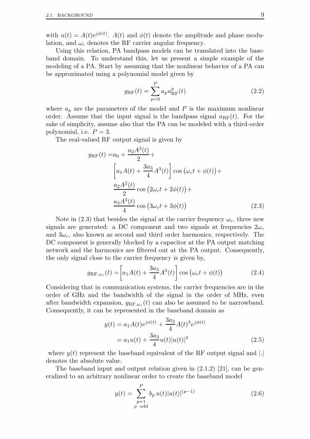
Using this relation, PA bandpass models can be translated into the base-band domain. To understand this, let us present a simple example of themodeling of a PA. Start by assuming that the nonlinear behavior of a PA canbe approximated using a polynomial model given by

yRF(t) =

P∑

p=0

apupRF(t) (2.2)

where ap are the parameters of the model and P is the maximum nonlinearorder. Assume that the input signal is the bandpass signal uRF(t). For thesake of simplicity, assume also that the PA can be modeled with a third-orderpolynomial, i.e. P = 3.

The real-valued RF output signal is given by

yRF(t) =a0 +a2A

2(t)

2+

[

a1A(t) +3a34

A3(t)

]

cos(

ωct+ φ(t))

+

a2A2(t)

2cos

(

2ωct+ 2φ(t))

+

a3A3(t)

4cos

(

3ωct+ 3φ(t))

(2.3)

Note in (2.3) that besides the signal at the carrier frequency ωc, three newsignals are generated: a DC component and two signals at frequencies 2ωc

and 3ωc, also known as second and third order harmonics, respectively. TheDC component is generally blocked by a capacitor at the PA output matchingnetwork and the harmonics are filtered out at the PA output. Consequently,the only signal close to the carrier frequency is given by,

yRF,ωc(t) =

[

a1A(t) +3a34

A3(t)

]

cos(

ωct+ φ(t))

(2.4)

Considering that in communication systems, the carrier frequencies are in theorder of GHz and the bandwidth of the signal in the order of MHz, evenafter bandwidth expansion, yRF,ωc(t) can also be assumed to be narrowband.Consequently, it can be represented in the baseband domain as

y(t) = a1A(t)ejφ(t) +

3a34

A(t)3ejφ(t)

= a1u(t) +3a34

u(t)|u(t)|2 (2.5)

where y(t) represent the baseband equivalent of the RF output signal and |.|denotes the absolute value.

The baseband input and output relation given in (2.1.2) [21], can be gen-eralized to an arbitrary nonlinear order to create the baseband model

y(t) =

P∑

p=1p odd

bp u(t)|u(t)|(p−1) (2.6)


where bp denotes the parameters of the model. This model is known as thebaseband polynomial model and is one of the simplest models used to charac-terize a PA.

From (2.6), it can be noticed that in the baseband representation of thepolynomial model only odd-order terms are present. The distortions producedby the even-order components are far from the carrier frequency and do notcontribute to the baseband output y(t) [22, 23]. However, in [24] it was shownthat better accuracy can be obtained if even-order terms are also considered.In this chapter, both even and odd order terms are used in the polynomial-based models.

Characterizing the PAs in the baseband domain reduces the computationalcomplexity, since the input and output signals can be acquired at lower sam-pling rates. Although bandpass behavioral models for PAs have been pro-posed in the literature, the majority of the behavioral models published areconstructed in the baseband domain. Consequently, all the models consideredin this chapter are of the baseband type.

2.2 Power amplifier baseband behavioral

models

According to the type of behavior they can represent, PA baseband behavioralmodels can be classified in three categories [2]: memoryless models, mod-els with linear memory and models with nonlinear memory. In this section,we present a review of the most commonly behavioral models in these cat-egories. For the description of those models, the instantaneous input andoutput complex-baseband signals of the PA are denoted by u(n) and y(n),respectively.

2.2.1 Memoryless models

Memoryless models are those that assume that the instantaneous output signaldepends only on the instantaneous input signal of the amplifier. These modelsare based on the quasi-static amplitude to amplitude conversion (AM/AM)and amplitude to phase conversion (AM/PM) properties of PAs. The AM/AMand AM/PM conversion represents the amplitude and phase distortion of theoutput signal as a function of the input signal amplitude.

Memoryless models can be easily extendable to model severe nonlinearities,but they can only provide acceptable accuracy when the PA presents few orno memory effects [2]. Various memoryless models have been proposed inthe literature. Among the most representative ones are: the power series orpolynomial model [2] which was derived in Section 2.1.2, and the look-up table(LUT) model.

The LUT model is the most basic technique to characterize the behaviorof PAs. LUTs derive the AM/AM and AM/PM conversions of a PA from rawmeasurement data using averaging or polynomial fitting and stores them intwo look-up tables [18]. For a given input amplitude, the LUT model indexesthe corresponding AM/AM and AM/PM conversion values and calculates the

2.2. POWER AMPLIFIER BASEBAND BEHAVIORAL

MODELS 11

x(n)Linear

filter

u(n)Static

nonlinearity

y(n)

(a)

x(n)Static

nonlinearity

u(n)Linear

filter

y(n)

(b)

Figure 2.2. Two-block model structures (a) Wiener model (b) Hammerstein model.

output as,y(n) = G(|u(n)|)u(n) (2.7)

where G(|u(n)|) is the instantaneous complex gain of the PA.

2.2.2 Nonlinear models with linear memory

Nonlinear models with linear memory are models that assume that the PAmemory effects can be modeled by using cascade combinations of linear filtersand a memoryless nonlinearity. According to the structure they used, thesemodels can be categorized as two-box, three-box and parallel-cascade models[2]. The most representative nonlinear models with linear memory are theWiener model and the Hammerstein model, illustrated in Fig. 2.2a.

The Wiener model is a two-box model comprised of a linear filter followedby a memoryless nonlinearity, as illustrated in Fig. 2.2a. The lowpass equiva-lent Wiener model is given by [2].

y(n) =

P∑

p=1

ap

[ M∑

m=0

hmu(n−m)

] M∑

m=0

∣

∣

∣

∣

hmu(n−m)

∣

∣

∣

∣

p−1

(2.8)

where P is the nonlinear order, M is the memory depth and ap and hm arethe model parameters. As can be noticed in (2.8), the Wiener model has theundesirable property to be nonlinear in the parameters hm, which makes theirparameter estimation more complicated than for models that are linear in theparameters [23].

The Hammerstein model is a two-box model composed of a memorylessnonlinear model followed by a linear filter, as depicted in Fig. 2.2b. Thecomplex baseband Hammerstein model is given by [2]

y(n) =

M∑

m=0

hm

[

P∑

p=1

ap u(n−m)|u(n−m)|p−1

]

(2.9)

where P is the nonlinear order, M is the memory depth and ap and hm arethe model parameters.

2.2.3 Nonlinear models with nonlinear memory

As the communication signals become more wideband, more accurate behav-ioral models that can account for the nonlinear memory effects are required.Throughout the years, several modeling approaches have been developed forthat purpose, such as polynomial-based models, the time-delay neural network


(TDNN) model and the nonlinear autoregressive moving-average (NARMA)model [2]. In this section, the focus is on polynomial-based models, due totheir ease of identification and use.

Volterra series

The Volterra series is a well-known mathematical tool used to represent theinput-output relationship of nonlinear dynamical systems including the non-linear behavior of PAs. The discrete complex-baseband Volterra series can beformulated as

y(n) =

P∑

p=1p odd

M∑

m1=0

M∑

m2=m1

. . .

M∑

m(p+1)/2=m(p−1)/2

M∑

(p+3)/2=0

. . .

M∑

mp=mp−1

hp(m1,m2, . . . ,mp)

(p+1)/2∏

i=1

u(n−mi)

p∏

(p+3)/2

u∗(n−mj) (2.10)

(2.11)

where hp(m1, . . . ,mp) are the parameters of the Volterra model and (.)∗ rep-resents the complex conjugate. P is the nonlinear order and M is the memorydepth. This model has the advantage of being linear in the parameters.

The Volterra series can provide good model accuracy, but unfortunatelythe number of parameters increases drastically with the nonlinear order andmemory depth. This limits the application of the Volterra series to weaklynonlinear PAs. In order to reduce the computational complexity, several mod-els have been developed to simplify its structure. These models are generallyknown as reduced Volterra or prunned Volterra models. A review of the mostcommonly used are presented in the next section.

Volterra-based models

The most commonly known reduced Volterra model is the memory polynomial(MP) model. Proposed in [25], the MP model can be seen as an extensionof the polynomial model to include memory or as a reduction of the Volterraseries in which only products with the same time-shifts are included [18]. TheMP model can be formulated as

y(n) =

P∑

p=1

M∑

m=0

apmx(n−m)|x(n −m)|p−1 (2.12)

where apm are the model parameters. P and M represent the maximumnonlinear order and the memory depth of the model, respectively.

Another important model in this category is the generalized memory poly-nomial (GMP) [23]. This model extends the MP model by also introducing

2.3. MODEL PARAMETER ESTIMATION 13

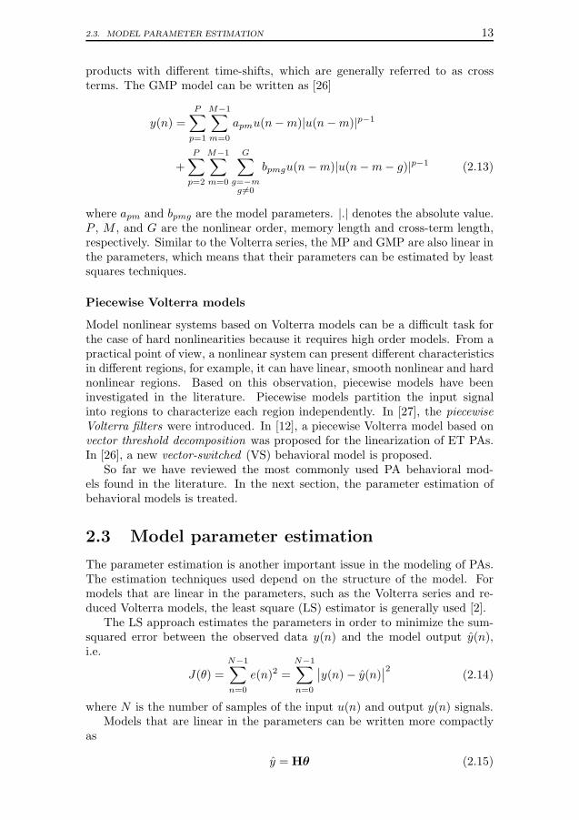
products with different time-shifts, which are generally referred to as crossterms. The GMP model can be written as [26]

y(n) =

P∑

p=1

M−1∑

m=0

apmu(n−m)|u(n−m)|p−1

+

P∑

p=2

M−1∑

m=0

G∑

g=−mg 6=0

bpmgu(n−m)|u(n−m− g)|p−1 (2.13)

where apm and bpmg are the model parameters. |.| denotes the absolute value.P , M , and G are the nonlinear order, memory length and cross-term length,respectively. Similar to the Volterra series, the MP and GMP are also linear inthe parameters, which means that their parameters can be estimated by leastsquares techniques.

Piecewise Volterra models

Model nonlinear systems based on Volterra models can be a difficult task forthe case of hard nonlinearities because it requires high order models. From apractical point of view, a nonlinear system can present different characteristicsin different regions, for example, it can have linear, smooth nonlinear and hardnonlinear regions. Based on this observation, piecewise models have beeninvestigated in the literature. Piecewise models partition the input signalinto regions to characterize each region independently. In [27], the piecewiseVolterra filters were introduced. In [12], a piecewise Volterra model based onvector threshold decomposition was proposed for the linearization of ET PAs.In [26], a new vector-switched (VS) behavioral model is proposed.

So far we have reviewed the most commonly used PA behavioral mod-els found in the literature. In the next section, the parameter estimation ofbehavioral models is treated.

2.3 Model parameter estimation

The parameter estimation is another important issue in the modeling of PAs.The estimation techniques used depend on the structure of the model. Formodels that are linear in the parameters, such as the Volterra series and re-duced Volterra models, the least square (LS) estimator is generally used [2].

The LS approach estimates the parameters in order to minimize the sum-squared error between the observed data y(n) and the model output y(n),i.e.

J(θ) =

N−1∑

n=0

e(n)2 =

N−1∑

n=0

∣

∣y(n)− y(n)∣

∣

2(2.14)

where N is the number of samples of the input u(n) and output y(n) signals.Models that are linear in the parameters can be written more compactly

as

y = Hθ (2.15)


where y is a column vector containing the samples of the model output y(n),H is a matrix consisting of the basis function of the model, and θ is a columnvector containing the model parameters.

And the LS solution is given by [28]

θ = (HHH)−1HHy (2.16)

where y is a vector containing the samples of the observed output signal y(n)and (.)H denotes the complex conjugate.

For models that are nonlinear in the parameters, such as the Wiener andHammerstein models, a more complex iterative estimation process is requiredto estimate the parameters of the linear filter block and the static nonlinearityblock. Techniques to estimate the parameters of each block can be found in[2, 29, 30].

2.4 Performance metrics

Once the model has been constructed, it is important to have accurate metricsto assess its performance. Several metrics have been proposed for this purpose.This section presents some of the most commonly used performance metricsfor PA behavioral models and DPD.

Normalized Mean Square Error

The normalized mean square error (NMSE) is defined as

NMSE =

N−1∑

n=0

| y(n)− y(n)|2

N−1∑

n=0

|y(n)|2(2.17)

where y(n) denotes the measured signal at the PA output and y(n) denotesthe modeled output. Since the NMSE is dominated by the in-band error, it isused to evaluate the in-band performance of the model.

Adjacent Channel Error Power Ratio

The adjacent channel error power ratio (ACEPR) is a measure of the out-of-band modeling capabilities. The ACEPR is given by

ACEPR = maxm=1,2

[∫

(adj)m|E(f)|2

∫

ch.|Y (f)|2

]

(2.18)

where E(f) denotes the power spectrum of the error observed between themeasured output and the modeled output, i.e. e(n) = y(n) − y(n). The inte-gration in the numerator is done over the adjacent channel, and the integrationin the denominator is done over the transmission channel.

2.4. PERFORMANCE METRICS 15

Adjacent Channel Leakage Ratio

The adjacent channel leakage ratio (ACLR) is a performance metric used forDPD. It measures the power of the distortion components that are leaked intothe adjacent channel in relation to the power of the signal in the main channel[2]. The ACLR is defined as

ACLR = maxm=1,2

[∫

(adj)m|Y (f)|2

∫

ch.|Y (f)|2

]

(2.19)

where Y (f) denotes the power spectrum of the measured output signal y(n).The integration in the numerator is done over the adjacent channel thatpresents the largest power and the integration in the denominator is doneover the transmission channel. The ACLR is generally presented in dB.


Chapter 3

Digital predistortion

DPD is currently the most active research area for the linearization of PAsbecause it offers a good tradeoff between implementation complexity and per-formance. While the behavioral modeling of a PA consist of finding a functionthat describe its dynamic nonlinear behavior, the DPD synthesis consists ofidentifying the function of the inverse of that behavior. This chapter startswith a formulation of the DPD problem. Next, conventional predistorter pa-rameter identification techniques are reviewed. Thereafter, a novel parameteridentification technique based on iterative learning control is presented. Fi-nally, the performance of the proposed ILC based parameter identificationtechnique is compared to conventional parameter identification techniques.

3.1 Formulation of the digital predistortion prob-

lem

Graphically, the problem of DPD can be represented as in Fig. 3.1. Considera PA system defined by y(n) = FPA[u(n)]. For this system, the goal is tofind a predistorter function denoted by FPD[x(n), θ], so that the output y(n)from the cascade of the predistorter and PA system is as close as possible toa desired output response yd(n), where close is measured in the sense of anarbitrary norm. This can be formulated as an optimisation problem

θ = argminθ

∥

∥e(n)∥

∥ = argminθ

∥

∥yd(n)− FPA

[

FPD[yd(n), θ]]∥

∥ (3.1)

The synthesis of a digital predistorter consists mainly in two tasks: to selecta model structure to realise the predistorter function FPD, and to identify theparameters θ of that model. In the literature, it is common to find that modelstructures used to characterize the behavior of PA are also used as predistortermodels [18, 19, 21, 23, 25, 26]. An overview of common PA behavioral modelsare given in Section 2.2. The focus of the rest of this chapter will be onparameter identification techniques for digital predistorters.

17

18 CHAPTER 3. DIGITAL PREDISTORTION

yd(n) Predistorter

FDPD(·)

u(n)PA

FPA(·)

y(n)

e(n)

Figure 3.1. The digital predistortion problem.

x(n)Predistorter

u(n)PA

y(n)

z(n)

1G

d(n)

u(n)copyparameters

Postdistorter

Figure 3.2. Indirect learning architecture principle. This technique identifies a postdis-torter of the PA and uses it as predistorter.

3.2 Digital predistortion identification techniques

3.2.1 P th-order inverse

The pth-order inverse is a technique used to find the inverse of nonlinear sys-tems whose input-output relation can be described by the Volterra series [31].The p-th order inverse of a nonlinear system is defined as p-th order Volterrasystem that when connected in tandem with the nonlinear system, results ina Volterra system that is linear up to p-th nonlinear order.

The p-th order inverse has some drawbacks. Its derivation is computation-ally heavy and it does not consider terms higher than the p-th nonlinear order.Moreover, it presents stability problems when the linear part of the system isnot stable and causal [31]. For these reason, the p-th order inverse is nota popular technique to estimate the parameters of a predistorter. However,the p-th order inverse theory developed in [31] is sometimes used to supportthe operation principle of the indirect learning architecture which will be dis-cussed in the next section. This theory states that the p-th order pre-inverseof a Volterra system is identical to the post-inverse of [31] that system.

3.2.2 Indirect learning architecture

First introduced in [32] as a learning architecture to train neural networkcontrollers and later adopted in [33] for DPD synthesis, ILA is currently themost widely used technique to identify the parameters of digital predistorters.ILA is based on the inverse modeling approach, where a post-inverse of thePA is identified by using the PA output signal y(n) to model the PA inputu(n), as illustrated in Fig. 3.2. Once the post-inverse of the PA (also knownas postdistorter) has been identified, the parameters of the postdistorter arecopied to an identical model that is used as the predistorter [34].

3.2. DIGITAL PREDISTORTION IDENTIFICATION TECHNIQUES 19

Since ILA estimates a post-inverse rather than a pre-inverse, the minimiza-tion criteria used by ILA can be written as follows

θ = argminθ

∥

∥d(n)∥

∥ (3.2)

where d(n), as seen in Fig. 3.2, is given by

d(n) = u(n)− u(n)

= FPD[x(n), θ]− FPD[y(n)/G, θ] (3.3)

where FPD denotes the predistorter and postdistorter function. ILA is thenbased on the fact that if the error d(n) vanishes, i.e. d(n) = 0 [33, 21] then

FPD[x(n), θ] = FPD[y(n)/G, θ] (3.4)

and consequently,

y(n) = Gx(n). (3.5)

However, in general cases, d(n) will not vanish completely. The reasons for thisis that the predistorter model structure used may not be sufficiently accurateor the parameters of the predistorter model may not be estimated perfectly.For instance, the authors in [35] shown that if the parameters θ are estimatedusing least squares (LS), i.e.

θ = argminθ

∥

∥u− u∥

∥

2

2(3.6)

where ‖·‖22 denotes the L2-norm square, u and u are vectors containing all thesamples from u(n) and u(n) in Fig. 3.2, due to the presence of measurementnoise in the PA output signal y(n), the parameters estimates converge to abiased solution.

Assuming that the predistorter model is linear in the parameters, then u

can be written as

u = Hθ (3.7)

whereH is the regression matrix that contains the basis functions of the model.Then the LS solution is given by,

θ = (HHH)−1HHu (3.8)

If the output signal does not contain noise then the regression matrix will beonly a function of y, i.e. H = H(y). In real applications however the regressionmatrix will also be a function of the measurement noise, denoted here as w,i.e.

H = H(y +w) = Ho +He (3.9)

where Ho and He denotes the contribution of the output signal and the mea-surement noise, respectively. Then the LS solution will be given by

θ =(

(Ho +He)H(Ho +He)

)−1(Ho +He)

Hu. (3.10)


After some calculations, it is shown in [35] that the LS parameter estimatesare given by

θ =(

(HHo Ho)

−1)

HHo u+B (3.11)

where B is a bias term that depends on the measurement noise level, and isgiven by [35]

B = Yu−

{

X[I+X]−1

(HHo Ho)

−1

}

(HHo +He)u (3.12)

with

Y =(

HHo Ho

)−1HH

e (3.13)

X =(

HHo Ho

)−1(

HHe He

)

(3.14)

Gain normalization issue in ILA

A critical issue encountered in ILA is that of the normalization gain selection[36, 37]. The normalization gain G is the scaling factor used to normalizethe output signal y(n) to the same power of the predistorter input signalx(n), as shown in Fig. 3.2. In the literature, different ways to compute thenormalization gain have been proposed. Some of the most commonly knownchoices are:

1. The maximum gain of the PA Glin [38], i.e. the gain of the PA when itoperates in its linear region.

2. The gain at the maximum targeted output power Gpeak [36].

3. The gain adjustment technique based on power alignment [37], in whichthe normalization gain is adjusted in order to find a value that does notvary the average input power to the PA.

The main issue with the normalization gain is that its selection affects theoutput power of the linearized amplifier. To better illustrate this, Fig. 3.3presents the NMSE and ACLR results of the linearization of a Class AB PAusing different normalization gain values. As noticed from this figure, the useof different normalization gain values produced output signals with differentaverage powers. Although the goal of DPD is to improve the linearity, it mustalso consider the output power of the PA. In order to properly evaluate theperformance of a predistorter, it is required that the PA average output powerobtained before DPD is not changed after DPD is applied [36]. To achievethis, the normalization gain must be carefully selected, which usually requiresadditional measurements and extra calibration efforts.

In order to overcome this issue, in Paper [A] a new variant to the ILA thateliminates the normalization gain block is proposed. As shown in Fig. 3.4, theproposed ILA variant uses the desired PA output response yd(n) as input tothe predistorter. Since the output signal from the PA y(n) and input signalto the predistorter yd(n) have similar power levels, no gain normalization atthe PA output is required. Any power mismatch between those signals is

3.2. DIGITAL PREDISTORTION IDENTIFICATION TECHNIQUES 21

30.5 31 31.5 32 32.5

−50

−40

−30

−20

w/o DPD

with DPD

Avg. Pout [dBm]

NM

SE

/AC

LR [d

B/d

Bc]

0.9*Gpeak

Gpeak 1.2*G

peak 1.4*Gpeak

NMSEACLR

Figure 3.3. NMSE and ACLR results versus average output power obtained using differentnormalization gain values. Note that the use of different normalization gain values produceoutput signal with different average powers.

yd(n)Predistorter

u(n)PA

y(n)

d(n)

u(n)copyparameters

Postdistorter

Figure 3.4. Proposed variant to the indirect learning architecture. Unlike the conventionalindirect learning architecture, this variant eliminates the normalization gain and uses thedesired PA output response as input to the predistorter.

31 31.5 32 32.5

−50

−40

−30

−20NMSE w/o DPD

NMSE with DPD

ACLR w/o DPD

ACLR with DPD

Avg. Pout [dBm]

NM

SE

/AC

LR [d

B/d

Bc]

Figure 3.5. NMSE and ACLR results versus average output power obtained using theproposed ILA variant. Note that the average output power obtained before DPD does notchange after DPD.


yd(n)Predistorter

u(n)PA

y(n)

Adaptive

Algorithm

yd(n)

e(n)

Figure 3.6. Direct learning architecture principle. This technique uses complex algorithmsto directly estimate the parameters that minimize e(n).

directly handled by ILA. When ILA converges, the PA output is driven toy(n) ≈ yd(n).

To evaluate the performance of the proposed ILA variant, it was usedto linearize a Class AB PA using desired output signals yd(n) with differentaverage output powers. The linearity results obtained before and after DPDare shown in Fig. 3.5. Note that since in the proposed ILA variant the desiredoutput response is defined before DPD is applied, the average output powerof the linearized PA matches the average output power obtained before DPDis applied for all the desired output signals tested.

3.2.3 Direct learning architecture

Another popular technique used to identify the parameters of a predistorteris the direct learning architecture (DLA), illustrated in Fig. 3.6. DLA is char-acterized for directly minimizing the error between the desired output signalyd(n) and the actual output from the amplifier y(n), i.e. e(n) = yd(n)− y(n)DLA uses complex optimization algorithms to estimate the parameters of thepredistorter. Various DLA algorithms have been proposed in the literature[39, 40, 41], unfortunately they are complex in structure, computationally ex-pensive and present slow convergence.

DLA is generally implemented in two steps [39, 40]. First a forward modelof the PA is identified. Once the model is obtained, a nonlinear algorithmis used to estimate, through iterative processing, the predistorter parametersthat minimize the error between the desired output and the PA model output.Once the nonlinear algorithm finds a solution, the estimated parameters areused to generate a predistorted signal u(n) that is applied to the real PA. Thisprocess is repeated iteratively until the predistorter-PA system converges tothe best possible solution.

3.3 Iterative learning control for the lineariza-

tion of power amplifiers

An important issue encountered in DPD linearization has always been thatthe desired output signal of the predistorter is unknown. For this reason,the parameters of predistorters are identified using the techniques presentedbefore. In order to overcome this issue, in [Paper B], a new identification

3.3. ITERATIVE LEARNING CONTROL FOR THE LINEARIZATION OF POWER AMPLIFIERS23

Learning

Controller

uk+1(n)

PA

uk(n)

System

yk(n)

ek(n)

yd(n)

Figure 3.7. Iterative learning control scheme for power amplifiers.

technique based on iterative learning control (ILC) named ILC-based DPD(ILC-DPD) is presented. This section describes the ILC concept and presentsan ILC scheme for the linearization of PAs

3.3.1 Iterative Learning Control

ILC is well-established control theory technique used to improve the transientresponse and tracking performance of systems that operate repetitively [42]and is also a powerful technique to obtain the inverse of nonlinear systems[43].

ILC is based on the observation that if the operating conditions of a sys-tem are the same each time it is executed, any errors observed in the outputresponse will be repeated every time the system is executed. Those errors canthen be used to refine the input signal so that the errors are reduced the nexttime the system is operated [42].

ILC scheme

A block diagram of the proposed ILC scheme for the linearization of PAs isillustrated in Fig. 3.7, where the subscript k is used to indicate the iterationnumber. The ILC scheme works as follows: During the k-th iteration thePA is driven by an input uk(n) which produces an output yk(n). A learningcontroller then uses the error observed between the desired and actual outputek(n) = yd(n) − yk(n) and the current input signal uk(n) to compute the anew input uk+1(n) that will be used during the next iteration. The learningalgorithm used by the learning controller is designed so that the error ek(n) isreduced after each iteration of the system. This process is repeated iterativelyuntil a desired performance is reached [42].

Learning algorithms

The main task in the design of an ILC scheme is to derive the learning al-gorithm that finds the optimal input u∗(n) that minimizes the error betweenthe desired output and actual output of the PA, i.e. ek(n) in Fig. 3.7. Paper[B] presents the derivation of two novel learning algorithms for the lineariza-tion of PAs: the instantaneous gain-based ILC algorithm and the linear ILCalgorithm.


The instantaneous-gain based algorithm is given by

uk+1 = uk +G(uk)−1ek (3.15)

where uk = [uk(0), uk(1), . . . , uk(N−1)] and ek = [ek(0), ek(1), . . . , ek(N−1)]respectively. G(uk) is a diagonal matrix given by

G(uk) = diag{

G[uk(0)], . . . , G[uk(N − 1)]}

(3.16)

where G[uk(n)] is the instantaneous complex gain of the PA which is definedby

G[uk(n)] =yk(n)

uk(n)(3.17)

The linear ILC algorithm is given by

uk+1 = uk + γek (3.18)

where γ is denoted as the learning gain. As shown in Paper [B], the convergenceof this algorithm is guaranteed if γ satisfies the following condition

0 < γ <2

Jmax

(3.19)

where Jmax denotes the supremum of the diagonal entries of the Jacobianmatrix of the PA with respect to uk. For PAs, Jmax is approximately equalto the small-signal gain of the amplifier which can be obtained from the PAdatasheet or easily calculated from measurements.

In order improve the convergence speed of the learning algorithms, theinput signal used during the first iteration u1(n) can be chosen as

u1(n) =yd(n)

gavg(3.20)

where gavg is the average gain of the amplifier at the desired average outputpower, which can be calculated from preliminary measurements.

The ILC scheme proposed for the linearization of PAs is summarized asfollows

1. Select yd

2. Set k = 1 and let u1 = yd/gavg, where gavg is the PA average gain atthe desired average output power

3. Apply uk to the PA and measure yk

4. Compute the error as ek = yd − yk

5. If ek satisfies the requirements, stop, otherwise continue

6. Compute uk+1 using the instantaneous gain-based (3.17) or the linearILC algorithms (3.18)

7. Let k = k + 1 and go to step 3

3.4. IDENTIFICATION TECHNIQUES PERFORMANCE COMPARISON 25

ILC

scheme

yd(n) u∗(n)

System

identification

copymodel

Predistorter design

Digital predistortion

Predistorter

u∗(n)yd(n)PA

y(n)

Figure 3.8. Block diagram of the iterative learning control based digital predistortiontechnique. In this technique, the ILC scheme described in section 3.3.1 is first used on thepower amplifier to identify the optimal input signal u∗(n) that drives the output to thedesired response yd(n). After that, yd(n) and u∗(n) are used to identify a predistortermodel. Finally, the identified model can be used as predistorter.

3.3.2 Iterative learning control based digital predistor-

tion

Although ILC can identify the optimal input signal u∗(n) that linearizes thePA, it does not provide a predistorter model. To alleviate this problem, anILC-DPD is proposed. The block diagram of ILC-DPD is shown in Fig. 3.8.ILC-DPD first uses an ILC scheme to find the optimal input signal u∗(n) thatdrives the PA to the desired output response yd. Once the optimal input signalu∗(n) is identified, the parameters of the predistorter model are estimatedusing yd(n) as model and u∗(n) as model output.

In principle, any PA behavioral model proposed in the literature can beused in ILC-DPD. But, it is not only limited to them. The true potential ofILC-DPD is that for the first time, we can get access to the optimal input signalthat drives the PA to the desired output response. ILC-DPD can be used incombination with any other modeling approaches to select and derive propermodel structures for PA predistorter, instead of relying on the assumption thatPA models and predistorter have the same structure [44].

3.4 Identification techniques performance com-

parison

In this section the performance of the identification techniques discussed inthis chapter are evaluated and compared to each other in two experimentalscenarios. In the first scenario, the linearization performance of ILA, DLAand ILC-DPD is evaluated when the output signal contains different levels ofmeasurement noise. In the second scenario, the performance of ILA, DLA,ILC and ILC-DPD is evaluated when the PA is in high compression.

The PA under test was a Cree CGH40006 GaN high-electron mobility tran-sistor (HEMT) mounted in the manufacturer’s board. The PA had a maximumpeak output power of 40.2 dBm at a frequency of 2 GHz. The signal used inthe experiments was a 5 MHz LTE signal with a PAPR of 8.5 dB and 25 MHzsampling rate.


The ILA scheme used in the experiments, was the proposed ILA variantshown in Fig. 3.4. For DLA, the predistorter parameters were estimated usingMATLAB’s nonlinear least squares algorithm solver, i.e the “lsqnonlin” func-tion. The performance is compared in terms of the NMSE between the desiredoutput signal and the actual output signal from the PA, and the ACLR.

3.4.1 Scenario I: Performance under various levels of mea-

surement noise

In this scenario, the performance of ILA, DLA and ILC-DPD is evaluated whenthe acquired output signal contains different levels of measurement noise, i.e.different SNR values. The PA was driven to an output power of 37 dBm. Thedifferent measurement noise levels were obtained by setting a high referencelevel and changing the attenuation in the spectrum analyzer (SA). To evaluatethe performance at the PA output, coherent averaging with 1000 repetitionswas applied to the output signals acquired by the SA. Then, the average outputsignal was used to compute the NMSE and ACLR. The predistorter parameterswere estimated using the signals acquired by the SA. The ILC algorithm usedwas the instantaneous-gain ILC algorithm given in 3.15. The model used inthe predistorter was a GMP model with nonlinear order P = 9, memory depthM = 1 and lagging term G = 1.

The NMSE and ACLR results for different SNR values are shown in Fig. 3.9and Fig. 3.10, respectively. Note that since the NMSE and ACLR performancedepend on the SNR of the output signal used in the parameter identification,the SNR values depicted in Fig. 3.9 and Fig. 3.10 correspond to the SNR ofthe output signals acquired by the SA.

From the three techniques, ILA presents the higher NMSE and ACLRresults for all the SNR values tested. In terms of NMSE, ILC-DPD presentsslightly lower results than DLA for SNR values of 20 dB. For SNR valuesbelow 20 dB the performance of ILC-DPD and DLA degrades rapidly. Withrespect to ACLR, ILC-DPD presents lower results than DLA for all the SNRvalues tested. These results indicate that ILC-DPD and DLA are more robustto measurement noise than ILA. They also show that ILC-DPD can achievebetter NMSE and ACLR performance than DLA when the measured outputsignal contains low SNR values, and can achieve those results using a lesscomplex identification process.

3.4.2 Scenario II: Performance under high compression

In this scenario, the performance of ILA, DLA, ILC and ILC-DPD are evalu-ated when the PA is driven in hard compression. The amplitude to amplitude(AM/AM) and amplitude to phase (AM/PM) conversion characteristics of thePA before DPD is applied is shown in Fig. 3.11. The algorithm used in ILCwas the linear ILC algorithm given in (3.18). The model used in the predis-torter was a GMP model with nonlinear order P = 9, memory depth M = 2and lagging term length G = 1.

Fig. 3.12 presents the power spectrum of the PA output signal obtainedbefore DPD, ILC-DPD, ILA and DLA for the evaluation data. Fig. 3.12 alsoincludes the power spectrum of the output signal obtained using ILC for the


10 15 20 25 30 35 40−45

−40

−35

−30

−25

−20

−15

NM

SE

(dB

)

Estimated SNR (dB)

No DPDILADLAILC−DPD

Figure 3.9. NMSE versus estimated signal-to-noise ration (SNR) obtained without DPD,ILA, DLA and ILC-DPD.

10 15 20 25 30 35 40−55

−50

−45

−40

−35

−30

AC

LR (

dBc)

Estimated SNR (dB)

No DPDILADLAILC−DPD

Figure 3.10. ACLR versus estimated signal-to-noise ration (SNR) obtained without DPD,ILA, DLA and ILC-DPD.


5 10 15 20 25 30 356

8

10

12

14

Input Power (dBm)A

M/A

M (

dB)

5 10 15 20 25 30 35−20

−10

0

10

20

Input Power (dBm)

AM

/PM

(D

egre

es)

Figure 3.11. Amplitude to amplitude (AM/AM) and amplitude to phase conversion(AM/PM) properties of the PA measured before DPD is applied.

identification data. The NMSE and ACLR results are summarized in Table3.1.

Before DPD, the NMSE and ACLR performance was -17.9 dB and -32.4dBc, respectively. When ILC was used, the NMSE and ACLR were improvedto -47.9 dB and -58.6 dBc, which represents an improvement of 30 dB and 26dB, respectively. The linearity improvement can be better noticed in Fig. 3.12,where the power leaked to the adjacent channels almost reaches the floor noiselevel. When ILC-DPD was used, the NMSE and ACLR obtained were -41.5 dBand -50.2 dBc, respectively, 7 dB and 10 dB higher than the results obtainedusing ILC. This performance degradation is attributed to the limited modelingcapabilities of the model used in the predistorter. When ILA was used, theNMSE and ACLR were -39 dB and -48 dBc, 1.5 dB and 2 dB higher thanILC-DPD. When DLA was used, the NMSE and ACLR were -41.8 dB and-50.9 dBc, respectively, 0.3 dB and 0.7 dB lower than the results obtainedwith ILC-DPD.

These results indicate that ILC can indeed identify the optimal PA in-put signal that linearizes the PA. This is because ILC focuses on identifyingan input signal rather than a predistorter model. ILC-DPD provided lowerperformance than ILC, but that performance depends on the modeling capa-bilities of the predistorter model. DLA provided slightly better performancethan ILC-DPD, but it uses a complex identification process and had slowconvergence. ILA presented the worst NMSE and ACLR numbers of all thetechniques tested.

It is important to highlight that although ILC-DPD uses the same de-sired output signal during each iteration, it can also be adapted into real-timeadaptive techniques. For instance, similar to the implementation of DLA, ILC-DPD could be applied to a model of the PA. Alternatively, the predistortermodel could be estimated after only one iteration of the ILC algorithm. Oncea predistorter model is obtained, the system could be operated with any newdesired output signal, and the predistorter parameters could be adapted withiterations on the predistorter-PA system, in a similar way to ILA.


−12.5 −7.5 −2.5 2.5 7.5 12.5−60

−45

−30

−15

0

Baseband Frequency (MHz)

PS

D (

dBx/

Hz) No DPD

ILA

ILC−DPD

ILC DLA

Figure 3.12. Power spectral density (PSD) of the measured PA output signal obtainedwithout DPD, and after applying ILC, ILA, DLA, and ILC-DPD for a Class B PA drivenunder high compression.

Table 3.1. Summary of the linearization results obtained when the PA was driven underhigh compression

Ident. Ident. Valid. Valid.DPD NMSE ACLR NMSE ACLRtype (dB) (dBc) (dB) (dBc)

w/o-DPD -17.97 -32.42 -18.05 -32.15ILC -47.96 -58.62 - -

ILC-DPD -41.52 -50.16 -40.62 -49.96ILA -39.85 -48.68 -39.04 -48.17DLA -41.81 -50.94 -41.07 -50.56


Chapter 4

Linearization of dual-input

power amplifier

architectures

The quest for improving the efficiency and performance of PAs has lead RFdesigners to develop transmitter architectures with dual inputs. But, in orderto be considered for practical applications, they need dedicated linearizationschemes that allow them to fulfill the stringent linearity requirements im-posed by regulatory agencies. This chapter discusses the linearization of thiskind of transmitter architectures. The first section describes some dual-inputtransmitter architectures. The second section presents digital predistortionlinearization schemes developed specially for this kind of transmitter architec-tures. And finally, the last section focuses on the linearization of dual-inputDoherty PAs.

4.1 Dual-input power amplifier architectures

This section reviews the varactor-based dynamic load modulation (DLM) PAarchitecture and the dual-input Doherty PA.

4.1.1 Varactor-based dynamic load modulation power am-

plifier architecture

Initially proposed in [8], the varactor-based DLM PA architecture is a fairlyrecent high-efficient PA architecture based on the dynamic load modulationprinciple. This architecture uses an electronically tunable matching networkthat can vary the instantaneous load impedance seen at the PA output, asshown in Fig. 4.1.

From the efficiency perspective, to be able to dynamically vary the PA loadimpedance is beneficial because it allows us to provide the PA with output loadimpedance values that enhances the efficiency at different output power levels.From the linearization perspective, however, to control this architecture, two

31

32 CHAPTER 4. LINEARIZATION OF DUAL-INPUT POWER AMPLIFIER ARCHITECTURES

yd DSP

unit

xDAC LPF

Up-converter

RFPA

Tunable

Matching

Network

RFoutput

vcDAC LPF

Baseband

yADC LPF

Down-converter

Figure 4.1. Block diagram of the varactor-based dynamic load modulation transmitterarchitecture

yd DSP

unit

xpDAC LPF

Up-converter

RFPA

Peaking

RFoutput

xmDAC LPF

Up-converter

RFPA

Main

yADC LPF

Down-converter

Figure 4.2. Simplified block diagram of the dual-input Doherty power amplifier.

signals must be generated in the digital domain: one complex-baseband signalx to drive the PA, and one real-valued baseband signal vc to control the tunablematching network, as can be seen in Fig. 4.1.

Although the varactor-based DLM has not yet gained the same attention asother PA architectures, promising results have been reported in the literature.In [16], a modular implementation of the varactor-based DLM, where the PAand tunable matching networks are designed separately is presented. Staticmeasurement results show that by using a tunable matching network, thepower-added efficiency can be improved by 10% at 10 dB back-off. In [45],it was shown that the varactor-based DLM may also be used to handle theeffects of antenna mismatch.

4.1.2 Dual-input Doherty power amplifier

Also referred to as the digital Doherty PA, the dual-input Doherty PA isa promising PA architecture for current and future wireless communicationsystems. Dual-input Doherty PAs eliminate the analog input splitter foundin Doherty PAs to allow independent control of the inputs to the main andpeaking amplifiers, as illustrated in Fig. 4.2. From the efficiency perspective,this action is beneficial because it allows the efficient distribution of inputpower to the main and peaking amplifiers to minimize the waste of power whenthe peaking amplifier is off, and to ensure the proper active load modulationwhen the two amplifiers are conducting [14]. From the bandwidth perspective,having two inputs allows independent control of the phase difference betweenbranches at different frequencies which enables frequency reconfiguration andwider bandwidth implementations [10]. From the linearization perspective,

4.2. LINEARIZATION SCHEMES 33

since two RF signals are needed to control this amplifier, the linearizer mustgenerate two complex-baseband signals, one to control the main PA xm andthe other to control the peaking PA xp.

4.2 Linearization schemes

As discussed in the previous section, dual-input transmitter architectures pro-vides an extra degree of freedom that can be used to enhance their efficiency.The goal of DPD is then to use that extra degree of freedom to simultane-ously optimize their linearity and efficiency. In this section, DPD linearizationschemes for dual-input PA architectures are described.

4.2.1 Efficiency-optimized static splitter

The efficiency-optimized static splitter, also referred to as static inverse modelsplitter, is the simplest way to control a dual-input PA architecture and en-hance its efficiency performance. The static splitter provides control functionsthat map any desired output signal to signals that control both branches ofthe PA architecture [16], as illustrated in Fig. 4.4.

The efficiency-optimized static inverse model is derived based on staticmeasurements where the dual-input PA architecture is driven with differentcombinations of the input parameters that influence their output to record theresulting output signals y and efficiency numbers. For the varactor-based DLMPA architecture, the parameters to vary are the input amplitude of the PA,|x|, and the baseband control signal vc, while for dual-input Doherty PAs theparameters are the input amplitudes of the main and peaking PAs |xm|, |xp|,and the phase difference between branches ∆φ. Fig. 4.3a, shows an exampleof the static measurements results obtained for a dual-input Doherty PA.

Since different combinations of those parameters may provide the sameoutput power but different efficiency results, a search is performed to findthe input parameters that optimize the efficiency at each output power level.Fig. 4.3b presents a plot the efficiency-optimized input parameters obtainedfor a dual-input Doherty PA. Using polynomial fitting, the resulting valuesare used to identify control functions that map any desired output signal ydto control signals for the dual-input PA architecture.

For the varactor-based DLM PA architecture, for the remaining of this the-sis, f1 and f2 will be used to denote the efficiency-optimized control functionsfor the RF branch and baseband branch, respectively.

x = f1(yd), vc = f2(yd) (4.1)

For the dual-input Doherty PA, the notation fm and fp will be used for theefficiency-optimized control functions for the main amplifier branch and peak-ing amplifier branch, respectively.

xm = fm(yd), xp = fp(yd) (4.2)

While the efficiency-optimized static inverse model can generate input sig-nals that ensure high-efficiency operation, it only considers the static nonlin-


10.5 21 31.5 420

20

40

60

80

Output power [dBm]

PA

E [%

]

(a)

0 11 22 33 440

3

6

9

12

Output Amplitude |y| [V]

Inpu

t Am

plitu

de [V

]

|xmopt|

|xpopt | ∆φopt

6 y

0 11 22 33 44−90

0

90

180

270

Pha

se [d

egre

es]

(b)

Figure 4.3. Static measurement results for a dual-input Doherty power amplifier (a)power added efficiency (PAE) results versus output power. Each blue dots corresponds to acombination of |xm|, |xp| and ∆φ. The red line correspond to the parameters combinationsthat optimizes the efficiency at each output power level. (b) efficiency-optimized inputparameters and phase of the output signal ∠y versus amplitude of the output signal.

DPD

yd y

Static Splitter

f1

Main

x

f2vc

DLMy

P

(a)

DPD

yd y

Static Splitter

fm

Main

xm

fp

Peaking

xp

y

(b)

Figure 4.4. Single-input linearization technique for (a) varactor-based dynamic load mod-ulation power amplifier (b) dual-input Doherty power amplifier.

earity of the PA architecture; consequently it can only compensate the dis-tortion to a limited extent. Moreover, since the control functions are realizedusing polynomial functions, fitting errors are always introduced.

4.2.2 Single-input linearization schemes

In order to compensate the memory effects and the static distortion causedby the imperfect control functions, the single-input linearization scheme com-bines the efficiency-optimized static-inverse model with a standard single-inputdigital predistorter model, as shown in Fig. 4.4.

This technique was proposed in [46] for the linearization of varactor-basedDLM PA architectures, but has also been applied to dual-input Doherty PAsin [47] and Paper [C]. Although this technique also considers the memoryeffects, the memory predistorter model cannot compensate the fitting errorsintroduced by the static splitter.

To overcome this problem, in [48] a modified single-input linearizationscheme was proposed for the varactor-based DLM PA architecture. As shownin Fig. 4.5, this technique introduces the memory predistorter only in the RFbranch. Although this technique can provide better linearity than the con-ventional single-input linearization scheme, the memory predistorter can only

4.2. LINEARIZATION SCHEMES 35

DPD

yd yStatic Splitter

f1x

f2vc

DLMy

P

Figure 4.5. Modified single-input linearization technique proposed for varactor-based dy-namic load modulation power amplifier.

compensate the fitting errors in the RF branch. Moreover, since each branchis controlled independently, these technique cannot guarantee optimized effi-ciency.

4.2.3 Dual-input linearization scheme

Another scheme developed for dual-input PA architectures is the dual-inputlinearization scheme. Initially derived in [49] for the linearization of varactor-based DLM architectures, this linearization scheme improves the linearity byusing the additional PA input signal as input to a dual-input predistorter. Ablock diagram of the dual-input linearization scheme is shown in Fig. 4.6a.

The dual-input linearization scheme is based on the assumption that if anappropriate envelope signal vc is given, then the transfer function of the PAfRF can be seen as a one-to-one mapping function between the RF input signalx and the output y signals, and can be inverted as

x = f−1RF(y, vc) (4.3)

where f−1RF is the inverse function between y and x only for a given vc. Thus,

(4.3) describes a set of inverse functions, one for each value of the variable vc.Moreover, if vc is chosen to optimize the efficiency, high linearity and efficiencycan be obtained simultaneously.

To generate vc, an efficiency-optimized function g is derived using staticmeasurements. The function g is equivalent to the control function f2, de-scribed in section 4.2.1.

In [49], the inverse function or predistortion function f−1RF was realized using

a modified 2-D GMP model, which is given by

x(n) = f−1RF [y(n), vc(n)] (4.4)

x(n) =

P∑

p=1

M−1∑

m=0

Pv∑

pv=0

Mv−1∑

mv=0

apmpvmvy(n−m)|y(n−m)|p−1vc(n−mv)pv

+

P∑

p=2

M−1∑

m=0

G∑

g=−mg 6=0

Pv∑

pv=0

Mv−1∑

mv=0

bpmgpvmvy(n−m)|y(n−m− g)|p−1vc(n−mv)pv

where apmpvmv and bpmgpvmv are the parameters of the model, P , M andG denote the nonlinear order, memory depth and crossterm length in the RFsignal y(n). Pv, Mv are the nonlinear order and memory depth in the envelope


DPD

yd x

g

P

vc

DLM

y

(a)

DPD

yd

Main

xm

f

Peaking

xp

y

(b)

Figure 4.6. Dual-input linearization technique for (a) varactor-based DLM and (b) dual-input DPA.

DPD

yd

fs

y

fsL

LPF

BW=fs

Static Splitter

fm

fp

LPFxm

LfsBW=fs

LPF

xp

LfsBW=fs

L

L

Main PA

xm

fs

Peaking PA

xp

fs

y

fs

Figure 4.7. Linearization scheme proposed to eliminate aliasing distortion caused by thehigh bandwidth of the control signals xm and xp in dual-input Doherty PAs. fs, L andBW denote the initial sampling rate, the upsampling factor and the available bandwidth,respectively.

signal vc. Note that this model extends the GMP model, in (2.13), to a dual-input model by adding a factor vc(n−mv)

pv to all the basis functions of theGMP model.

Since this scheme uses vc as second input to the predistorter, the fittingerrors in the baseband branch can be compensated by the dual-input predis-torter.

The dual-input linearization scheme was later adapted in [50] for the lin-earization of dual-input Doherty PAs, as shown in Fig. 4.6b. In that scheme,the efficiency-optimized control function f is derived for the peaking branchand is equivalent to the control function fp of the static splitter.

For varactor-based DLM PA architectures, in [49], it was shown that thedual-input linearization scheme can successfully linearize the PA architecturewhile maintaining high efficiency performance. For dual-input Doherty PAs[50], although this scheme provides better performance than the single-inputlinearization one, it cannot eliminate all the distortions introduced by thedual-input Doherty PA. In the following section, we will discuss more on thelinearization of this kind of PA architectures.

4.3 Linearization challenges in dual-input Do-

herty power amplifiers

In paper [C], different aspects of the linearization of dual-input Doherty PAsare investigated. The study is based on the single-input linearization schemedescribed in Section 4.2.2, using a vector-switched generalized memory poly-

4.3. LINEARIZATION CHALLENGES IN DUAL-INPUT DOHERTY POWER AMPLIFIERS 37

−12.5 −7.5 −2.5 2.5 7.5 12.5−80

−60

−40

−20

0

With VS−GMP DPD

Without DPD

Baseband Frequency [MHz]

Nor

mal

ized

PS

D [d

Bx/

Hz]

(a)

−12.5 −7.5 −2.5 2.5 7.5 12.5−80

−60

−40

−20

0

With VS−GMP DPD

Without DPD

Baseband Frequency [MHz]

Nor

mal

ized

PS

D [d

Bx/

Hz]

(b)

Figure 4.8. Linearization results (a) using a the single-input linearization with a VS-GMPmodel (b)using the scheme proposed in [Paper C]. Note that the proposed scheme can reducethe spectral regrowth at 12.5 MHz offset by more than 9 dB, even before applying DPD.

nomial (VS-GMP) model [26] as memory predistorter. The signal used inthe experiments was a 5 MHz LTE signal with a 8.5 dB PAPR and 25 MHzsampling rate.

The linearity results and spectrum of the output signals before and afterDPD are illustrated in Table 4.1 and Fig. 4.8a, respectively. As can be noticedfrom Table 4.1, good NMSE, ACLR and efficiency numbers can be obtainedusing the single-input linearization scheme and a VS-GMP model. However,as can be observed in Fig. 4.8a, there is some spectral regrowth towards theedges of the spectrum that cannot be eliminated.

The residual spectral regrowth indicate that there is aliasing distortion inthe signals obtained after the static splitter. This aliasing is generated becausethe bandwidth of the control signals is larger than the sampling rate used. Toovercome the aliasing distortion problem, the linearization scheme shown inFig. 4.7 was proposed in paper [C]. The proposed scheme upsamples the pre-distorted signal y L times before it is applied to the static splitter. The outputsignals from the static splitter are filtered to eliminate any components outsidethe bandwidth of interest, i.e BW = fs, where fs denotes the sampling rate.Thereafter, those signals are downsampled L times to the original samplingrate fs to then feed the main and peaking PAs. The linearization results andspectrum plots obtained using this scheme are shown in Fig. 4.8b and Table4.1. As seen from Fig. 4.8b, the residual spectral regrowth was reduced com-pared to the standard single-input linearization scheme. Even before DPD wasapplied the spectral regrowth at 12.5 MHz offset was reduced by more than9 dB. However, the spectral regrowth was not completely eliminated. Theseresults indicate that there are other factors that contribute to the residualspectral regrowth, e.g. the limited sampling rate or the limited capabilities ofthe predistorter model.

In order to find the effects that the sampling rate has on the residualspectral regrowth, the dual-input Doherty PA was also linearized using highersampling rates. The results are shown in Fig. 4.9 and Table 4.1. From Fig. 4.9,it can be noticed that the residual spectral regrowth is reduced as the samplingrate is increased. Moreover, if a sufficiently fast sampling rate is used all thedistortions can be eliminated. Unfortunately, in real applications, such fastsampling rates cannot be afforded because they require fast and power hungrydigital-to-analog converters (DAC) and analog to digital converters (ADC).


−50 −25 0 25 50−80

−60

−40

−20

0

Baseband Frequency [MHz]N

orm

aliz

ed P

SD

[dB

x/H

z]

fs=25MHz

fs=50MHz

fs=100MHz

Figure 4.9. Linearization results obtained using Fig. 4.4b and different sampling rates.Note that the residual spectral regrowth is reduced as the sampling rate is increased.

Table 4.1. Summary of the results of the linearization of a dual-input Doherty PA

DPD fs NMSE ACLR Pout PAEtype (MHz) (dB) (dBc) (dBm) (%)

Splitter a 25 -23.5 -30.7 33.3 43.8VS-GMPa 25 -43.1 -53.7 33.4 43.7Splitter b 25 -23.6 -31.0 33.3 42.4

VS-GMPb 25 -43.7 -55.8 33.3 42.4VS-GMPa 50 -46.6 -63.6 33.3 43.9VS-GMPa 100 -48.9 -64.7 33.3 43.9

a calculated using linearization scheme in Fig. 4.4b.b calculated using linearization scheme in Fig. 4.8.

These results indicate that there are mainly two limiting factors in thelinearization of dual-input Doherty PAs: the large bandwidth of the controlsignals and the limited sampling rate used. The linearization scheme proposedin paper [C] can provide an alternative to improve the linearity of dual-inputDoherty PAs without increasing the DAC and ADC requirements, but it can-not completely eliminate the residual spectral regrowth. Consequently, thelinearization of dual-input Doherty PAs over limited sampling rates remainsan open research problem. The ILC scheme proposed in paper [B] is a promis-ing technique to solve this problem, but we will discuss this in the future worksection.

Chapter 5

Conclusions and Future

Work

5.1 Conclusions

High efficiency and linear PAs are essential components in wireless communi-cations system. There is however a tradeoff between efficiency and linearity:high efficiency PAs behave nonlinearly and linear PA present low efficiency.In order to fulfill the efficiency and linearity requirements, DPD is often used.This thesis has contributed to different aspects of the linearization of PAs usingDPD.

The synthesis of a predistorter consists mainly in two tasks: the selectionor design of models to be used in the predistorter and the identification of theparameters of the model. For the parameter identification, techniques such asp-th order inverse, ILA and DLA have been proposed in the literature. Amongthem, ILA is the most widely used because it reduces the identification processto an iterative inverse-modeling process. But the adoption of ILA introducesa critical issue known as gain normalization. In the literature, there is not aclear consensus on how the normalization gain must be computed. We haveinvestigated this issue and have shown that the normalization gain affectsthe output power of the linearized PA. Therefore, it adds an extra degree offreedom, which must be carefully selected. To overcome this issue, we haveproposed a variation of ILA that eliminates the normalization gain block anduses the desired output response as input to the predistorter. Experimentsshowed that the proposed ILA variant allows a better control of the outputsignal from the linearized PA, since this signal depends only on the input signalto the predistorter, and not on the correct selection of a normalization gain.

An important issue encountered in DPD has been that the output signalfrom the predistorter that linearizes the PA is unknown. For this reason, theparameters of the predistorter are identified using techniques such as ILA andDLA. To overcome this issue, we have proposed a novel parameter identifica-tion technique based on ILC. To this end, we have designed an ILC scheme forthe linearization of PAs. Experimental results showed that the proposed ILCscheme can identify the optimal linearizing input signal. The experiments also

39

40 CHAPTER 5. CONCLUSIONS AND FUTURE WORK

showed that proposed identification technique can achieve better linearizationperformance than ILA and DLA when high levels of measurement noise arepresent and when the PA is in high compression. The ILC scheme and theidentification technique presented here have the potential to enable the designof model structures for digital predistorters.

The introduction of dual-input transmitter architectures have introducednew challenges to digital predistortion. In this work, we have studied lineariza-tion aspects of dual-input Doherty PAs and identified some of the associatedchallenges. We have experimentally shown that the large bandwidth of thecontrol signals and the limited sampling rates used in the linearization are twothe main factors that limit their linearity performance. We have addressedthis issue with a novel linearization scheme that provides a better linearitycompared to the existing schemes for a given sampling rate.

In summary, we have developed new concepts and methods for DPD lin-earization of PAs. These contributions are expected to make a broad impacton the realization of energy efficient and linear radio transmitters for emergingand future wireless systems.

5.2 Future Work

There are several lines of research arising from the work presented in this thesiswhich can be pursued. Since ILC can find the optimal linearizing input signal,it reduces the design of the predistorter to a modeling problem. It would beinteresting to use ILC together with other modeling and estimation techniquesto select or design model structures for digital predistorters. ILC and ILC-DPD could also be used for the linearization of dual-input Doherty PAs. Due tothe large bandwidth of the control signals and the limited sampling rates usedin the linearization, there is a residual distortion that cannot be compensatedusing standard modeling and estimation techniques. Since ILC focuses onidentifying an input signal rather than a model, it could be used to identifythe optimal control signals to the PA, to then design a suitable predistortermodel.

Acknowledgements

I would like express my gratitude to all the people that made this work possible.First and foremost, I would like to express my gratitude to my main advisorProf. Thomas Eriksson and co-advisor Adj. Prof. Christian Fager. I amindebted for the opportunity you have given me, and for the support andguidance you have provided, without your support this work would not havebeen possible. I would also like to thank my second co-advisor Dr. Per Landinfor your guidance and support and for all the many fruitful discussions onresearch and measurement problems.

I would like to thank Prof. Jan Grahn, director of the GigaHertz Centre,for creating such a good research environment and to Prof. Erik Strom, forproviding a pleasant working environment here in the Communication SystemsGroup.

Thanks to my colleagues at the Communication Systems Group and at theMicrowave Electronics Laboratory. Special thanks to Dr. Mustafa Ozen forhis support on RF measurements and for answering every single question onpower amplifiers. Thanks to Dr. David Gustafsson, for designing the dual-input power amplifier used in this work. I would also like to thank AgnetaKinnander and Karin Hallin for their help in administrative matters, and toLars Borjesson for the computer support.

Last but not least, I would like to thanks my family for their constantsupport, love and encouragements over the years. To Mr. Gustav, my cat, forbeing my furry little companion.

This research has been carried out in the Gigahertz Centre in a joint projectfinanced by the Swedish Government Agency for Innovation Systems (VIN-NOVA), Chalmers University of Technology, Ericsson AB, Gotmic AB, Infi-neon Technologies Austria AG, National Instruments, NXP SemiconductorsBV and SAAB AB.

41

42 CHAPTER 5. CONCLUSIONS AND FUTURE WORK

Bibliography

[1] P. Lavrador, T. Cunha, P. Cabral, and J. Pedro, “The linearity-efficiencycompromise,” IEEE Microw. Mag., vol. 11, no. 5, pp. 44–58, Aug. 2010.

[2] D. Schreurs, M. O’Droma, A. A. Goacher, and M. Gadringer, RF PowerAmplifier Behavioral Modeling. Cambridge, 2008.

[3] A. Mohammadi and F. M. Ghannouchi, RF Transceiver Design for MIMOWireless Communications. Springer Berlin Heidelberg, 2012.

[4] F. H. Raab, P. Asbeck, S. Cripps, P. B. Kenington, Z. B. Popovic,N. Pothecary, J. F. Sevic, and N. O. Sokal, “Power amplifiers and trans-mitters for RF and microwave,” IEEE Trans. Microw. Theory Tech.,vol. 50, no. 3, pp. 814–826, Mar. 2002.

[5] P. Draxler, S. Lanfranco, D. Kimball, C. Hsia, J. Jeong, J. van de Sluis,and P. M. Asbeck, “High efficiency envelope tracking LDMOS power am-plifier for W-CDMA,” in IEEE MTT-S Int. Microwave Symp. Dig., June2006, pp. 1534–1537.

[6] W. H. Doherty, “A new high efficiency power amplifier for modulatedwaves,” Proc. IRE, vol. 24, no. 9, pp. 1163–1182, Sept 1936.

[7] H. Chireix, “High power outphasing modulation,” Proc. IRE, 1935.

[8] F. H. Raab, “High-efficiency linear amplification by dynamic load modu-lation,” in IEEE MTT-S Int. Microwave Symp. Dig., vol. 3, June 2003,pp. 1717–1720.

[9] S. Cripps, RF Power Amplifiers for Wireless Communications. ArtechHouse, 2006.

[10] J. H. Qureshi, N. Li, W. C. E. Neo, F. van Rijs, I. Blednov, and L. C. N.de Vreede, “A wide-band 20W LDMOS Doherty power amplifier,” inIEEE MTT-S Int. Microwave Symp. Dig., May 2010, pp. 1504–1507.

[11] K. Chen and D. Peroulis, “Design of adaptive highly efficient GaN poweramplifier for octave-bandwidth application and dynamic load modula-tion,” IEEE Trans. Microw. Theory Tech., vol. 60, no. 6, pp. 1829–1839,June 2012.

43

44 BIBLIOGRAPHY

[12] A. Zhu, P. J. Draxler, C. Hsia, T. J. Brazil, D. F. Kimball, and P. M.Asbeck, “Digital predistortion for envelope-tracking power amplifiers us-ing decomposed piecewise Volterra series,” IEEE Trans. Microw. TheoryTech., vol. 56, no. 10, pp. 2237–2247, Oct 2008.

[13] R. Darraji, F. M. Ghannouchi, and O. Hammi, “A dual-input digitallydriven Doherty amplifier architecture for performance enhancement ofDoherty transmitters,” IEEE Trans. Microw. Theory Tech., vol. 59, no. 5,pp. 1284–1293, May 2011.

[14] R. Darraji and F. M. Ghannouchi, “Digital Doherty amplifier with en-hanced efficiency and extended range,” IEEE Trans. Microw. TheoryTech., vol. 59, no. 11, pp. 2898–2909, Nov. 2011.

[15] D. Gustafsson, C. M. Andersson, and C. Fager, “A modified Dohertypower amplifier with extended bandwidth and reconfigurable efficiency,”IEEE Trans. Microw. Theory Tech., vol. 61, no. 1, pp. 533–542, Jan. 2013.

[16] H. M. Nemati, C. Fager, U. Gustavsson, R. Jos, and H. Zirath, “Design ofvaractor-based tunable matching networks for dynamic load modulationof high power amplifiers,” IEEE Trans. Microw. Theory Tech., vol. 57,no. 5, pp. 1110–1118, May 2009.

[17] M. Isaksson, D. Wisell, and D. Ronnow, “A comparative analysis of be-havioral models for RF power amplifiers,” IEEE Trans. Microw. TheoryTech., vol. 54, no. 1, pp. 348–359, Jan. 2006.

[18] F. M. Ghannouchi and O. Hammi, “Behavioral modeling and predistor-tion,” IEEE Microw. Mag., vol. 10, no. 7, pp. 52–64, Dec 2009.

[19] L. Ding, “Digital predistortion of power amplifiers for wireless applica-tions,” Ph.D. dissertation, Georgia Institute of Technology, Atlanta, USA,2004.

[20] S. Haykin, Digital Communication Systems. Wiley, 2014.

[21] P. Landin, “Digital baseband modeling and correction of radio frequencypower amplifiers,” Ph.D. dissertation, KTH Royal Institute of Technology,Stockholm, Sweden, 2012.

[22] S. P. Stapleton and J. K. Cavers, “A new technique for adaptation oflinearizing predistorters,” in Veh. Technology Conf., May 1991, pp. 753–758.

[23] D. R. Morgan, Z. Ma, J. Kim, M. G. Z. Zierdt, and J. Pastalan, “Ageneralized memory polynomial model for digital predistortion of rf poweramplifiers,” IEEE Trans. Signal Process., vol. 54, no. 10, pp. 3852–3860,Oct. 2006.

[24] L. Ding and G. T. Zhou, “Effects of even-order nonlinear terms on poweramplifier modeling and predistortion linearization,” IEEE Trans. Veh.Technology, vol. 53, no. 1, pp. 156–162, Jan 2004.

BIBLIOGRAPHY 45

[25] J. Kim and K. Konstantinou, “Digital predistortion of wideband signalsbased on power amplifier model with memory,” Electron. Lett., vol. 37,no. 23, pp. 1417–1418, Nov. 2001.

[26] S. Afsardoost, T. Eriksson, and C. Fager, “Digital predistortion usinga vector-switched model,” IEEE Trans. Microw. Theory Tech., vol. 60,no. 4, pp. 1166–1174, Apr. 2012.

[27] E. A. Heredia and G. R. Arce, “Piecewise Volterra filters based on thethreshold decomposition operator,” in Int. Conf. on Acoust., Speech, andSignal Process., vol. 3, May 1996, pp. 1593–1596.

[28] S. M. Kay, Fundamentals of statistical signal processing, Volume 1: Esti-mation Theory. Pearsson, 1993.

[29] D. Silveira, M. Gadringer, H. Arthaber, and G. Magerl, “RF-power am-plifier characteristics determination using parallel cascade Wiener modelsand pseudo-inverse techniques,” in Microw. Conf. Proc., vol. 1, Dec 2005,pp. 4 pp.–.

[30] D. Silveira, M. Gadringer, H. Arthaber, M. Mayer, and G. Magerl., “Mod-eling, analysis and classification of a PA based on identified Volterra ker-nels,” in European Gallium Arsenide and Other Semiconductor Applicat.Symp., Oct 2005, pp. 405–408.

[31] M. Schetzen, The Volterra and Wiener Theorems of Nonlinear Systems.Wiley, 1980.

[32] D. Psaltis, A. Sideris, and A. A. Yamamura, “A multilayer neural networkcontroller,” IEEE Control Syst. Mag., 1988.

[33] C. Eun and E. J. Powers, “A new Volterra predistorter based on the in-direct learning architecture,” IEEE Trans. Signal Process., vol. 45, no. 1,pp. 223–227, Jan. 1997.

[34] D. R. Morgan, Z. Ma, and L. Ding, “Reducing measurement noise ef-fects in digital predistortion of RF power amplifiers,” in IEEE Int. Conf.Commun., vol. 4, May 2003, pp. 2436–2439.

[35] S. Amin, E. Zenteno, P. N. Landin, D. Ronnow, M. Isaksson, and P. Han-del, “Noise impact on the identification of digital predistorter parametersin the indirect learning architecture,” in Swedish Commun. TechnologiesWorkshop Dig., Oct. 2012, pp. 36–39.

[36] A. Zhu, P. J. Draxler, J. J. Yan, T. Brazil, D. F. Kimball, and P. M.Asbeck, “Open-loop digital predistorter for RF power amplifiers usingdynamic deviation reduction-based volterra series,” IEEE Trans. Microw.Theory Tech., vol. 56, no. 7, pp. 1524–1534, July 2008.

[37] O. Hammi and F. M. Ghannouchi, “Power alignment of digital predis-torters for power amplifiers linearity optimization,” IEEE Trans. Broad-cast., vol. 55, no. 1, pp. 109–114, March 2009.

46 BIBLIOGRAPHY

[38] K. J. Muhonen, M. Kavehrad, and R. Krishnamoorthy, “Look-up tabletechniques for adaptive digital predistortion: a development and com-parison,” IEEE Trans. Veh. Technol., vol. 49, no. 5, pp. 1995–2002, Sep2000.

[39] D. Zhou and V. E. DeBrunner, “Novel adaptive nonlinear predistortersbased on the direct learning algorithm,” IEEE Trans. Signal Process.,vol. 55, no. 1, pp. 120–133, Jan. 2007.

[40] H. Passo and A. Mammela, “Comparison of direct learning and indirectlearning predistortion architectures,” in IEEE Int. Symp. Wireless Com-mun. Syst., Oct. 2008, pp. 309–313.

[41] M. A. Hussein, V. A. Bohara, and O. Venard, “On the system level con-vergence of ILA and DLA for digital predistortion,” in Int. Symp. onWireless Commun. Syst., Aug. 2012, pp. 870–874.

[42] H. S. Ahn, K. L. Moore, and Y. Chen, Iterative Learning Control: Ro-bustness and Monotonic Convergence for Interval Systems. Springer,2007.

[43] O. Markusson, “Model and system inversion with applications in non-linear system identification and control,” Ph.D. dissertation, KTH RoyalInstitute of Technology, Stockholm, Sweden, 2002.

[44] M. Isaksson and D. Ronnow, “A parameter-reduced volterra model for dy-namic rf power amplifier modeling based on orthonormal basis functions,”in In press. In Press, 2007.

[45] C. Sanchez-Perez, J. de Mingo, P. Garcia-Ducar, P. L. Carro, and A. Val-dovinos, “Dynamic load modulation with a reconfigurable matching net-work for efficiency improvement under antenna mismatch,” IEEE Trans.Circ. and Systems II: Express Briefs, vol. 58, no. 12, pp. 892–896, Dec2011.

[46] H. Cao, H. M. Nemati, A. S. Tehrani, T. Eriksson, J. Grahn, andC. Fager., “Linearization of efficiency-optimized dynamic load modulationtransmitter architectures,” IEEE Trans. Microw. Theory Tech., vol. 58,no. 4, pp. 873–881, Apr. 2010.

[47] C. M. Andersson, D. Gustafsson, J. Chani-Cahuana, R. Hellberg, andC. Fager, “A 1-3-ghz digitally controlled dual-RF input power-amplifierdesign based on a doherty-outphasing continuum analysis,” IEEE Trans.Microw. Theory Tech., vol. 61, no. 10, pp. 3743–3752, Oct. 2013.

[48] H. M. Nemati, H. Cao, B. Almgren, T. Eriksson, and C. Fager, “De-sign of highly efficient load modulation transmitter for wideband cellularapplications,” IEEE Trans. Microw. Theory Tech., vol. 58, no. 11, pp.2820–2828, Nov 2010.

[49] H. Cao, H. M. Nemati, A. S. Tehrani, T. Eriksson, and C. Fager, “Digitalpredistortion for high efficiency power amplifier architectures using a dual-input modeling approach,” IEEE Trans. Microw. Theory Tech., vol. 60,no. 2, pp. 361–369, Feb. 2012.

BIBLIOGRAPHY 47

[50] H. Cao, J. Qureshi, T. Eriksson, C. Fager, and L. de Vreede, “Digitalpredistortion for dual-input doherty amplifiers,” in IEEE Topical Conf.on Power Amplifiers for Wireless and Radio Applications, Jan. 2012, pp.45–48.

48 BIBLIOGRAPHY

Paper A

A New Variant to the Indirect Learning Architecture

J. Chani Cahuana, C. Fager, T. Eriksson

in European Microwave Conference , France, Paris, Sep., 2015

©2015 IEEE

Paper B

Iterative Learning Control for the Linearization of Power

Amplifiers

J. Chani Cahuana, P. Landin, C. Fager, and T. Eriksson

Submitted to, IEEE Trans. Microw. Theory, Feb., 2015

Paper C

Linearization of Dual-Input Doherty Power Amplifiers

J. Chani Cahuana, P. Landin, C. Fager, and T. Eriksson

IEEE International Workshop on Integrated Nonlinear Microwaveand Milimetre-wave Circuits (INMMiC), Leuven, Belgium, Apr.

2014

©2014 IEEE

Date post:	30-Jul-2018
Category:	Documents
Upload:	haliem
View:	216 times
Download:	0 times

Digital Predistortion for the Linearization of Power … · the complexity of radio frequency (RF)...

Documents