271
PDF generated using the open source mwlib toolkit. See http://code.pediapress.com/ for more information. PDF generated at: Sat, 07 Jun 2014 14:28:26 UTC Digital Signal Processing
| Date post: | 19-Jan-2016 |
| Category: |
Documents |
| Upload: | pecmurugan |
| View: | 559 times |
| Download: | 21 times |

PDF generated using the open source mwlib toolkit. See http://code.pediapress.com/ for more information.PDF generated at: Sat, 07 Jun 2014 14:28:26 UTC
Digital Signal Processing
ContentsArticles
Digital signal processing 1Discrete signal 6
Sampling 8
Sampling (signal processing) 8Sample and hold 13Digital-to-analog converter 15Analog-to-digital converter 21Window function 32Quantization (signal processing) 53Quantization error 63ENOB 74Sampling rate 75Nyquist–Shannon sampling theorem 80Nyquist frequency 91Nyquist rate 93Oversampling 95Undersampling 97Delta-sigma modulation 99Jitter 112Aliasing 117Anti-aliasing filter 122Flash ADC 124Successive approximation ADC 126Integrating ADC 129Time-stretch analog-to-digital converter 137
Fourier Transforms, Discrete and Fast 142
Discrete Fourier transform 142Fast Fourier transform 157Cooley-Tukey FFT algorithm 165Butterfly diagram 171Codec 173FFTW 175
Wavelets 177
Wavelet 177Discrete wavelet transform 188Fast wavelet transform 196Haar wavelet 198
Filtering 205
Digital filter 205Finite impulse response 211Infinite impulse response 218Nyquist ISI criterion 221Pulse shaping 223Raised-cosine filter 225Root-raised-cosine filter 228Adaptive filter 229Kalman filter 234Wiener filter 255
Receivers 260
ReferencesArticle Sources and Contributors 261Image Sources, Licenses and Contributors 265
Article LicensesLicense 268
Digital signal processing 1
Digital signal processingDigital signal processing (DSP) is the mathematical manipulation of an information signal to modify or improve itin some way. It is characterized by the representation of discrete time, discrete frequency, or other discrete domainsignals by a sequence of numbers or symbols and the processing of these signals.The goal of DSP is usually to measure, filter and/or compress continuous real-world analog signals. The first step isusually to convert the signal from an analog to a digital form, by sampling and then digitizing it using ananalog-to-digital converter (ADC), which turns the analog signal into a stream of numbers. However, often, therequired output signal is another analog output signal, which requires a digital-to-analog converter (DAC). Even ifthis process is more complex than analog processing and has a discrete value range, the application of computationalpower to digital signal processing allows for many advantages over analog processing in many applications, such aserror detection and correction in transmission as well as data compression.Digital signal processing and analog signal processing are subfields of signal processing. DSP applications include:audio and speech signal processing, sonar and radar signal processing, sensor array processing, spectral estimation,statistical signal processing, digital image processing, signal processing for communications, control of systems,biomedical signal processing, seismic data processing, etc. DSP algorithms have long been run on standardcomputers, as well as on specialized processors called digital signal processor and on purpose-built hardware such asapplication-specific integrated circuit (ASICs). Today there are additional technologies used for digital signalprocessing including more powerful general purpose microprocessors, field-programmable gate arrays (FPGAs),digital signal controllers (mostly for industrial apps such as motor control), and stream processors, among others.Digital signal processing can involve linear or nonlinear operations. Nonlinear signal processing is closely related tononlinear system identification [1] and can be implemented in the time, frequency, and spatio-temporal domains.
Signal samplingMain article: Sampling (signal processing)With the increasing use of computers the usage of and need for digital signal processing has increased. To use ananalog signal on a computer, it must be digitized with an analog-to-digital converter. Sampling is usually carried outin two stages, discretization and quantization. In the discretization stage, the space of signals is partitioned intoequivalence classes and quantization is carried out by replacing the signal with representative signal of thecorresponding equivalence class. In the quantization stage the representative signal values are approximated byvalues from a finite set.The Nyquist–Shannon sampling theorem states that a signal can be exactly reconstructed from its samples if thesampling frequency is greater than twice the highest frequency of the signal; but requires an infinite number ofsamples. In practice, the sampling frequency is often significantly more than twice that required by the signal'slimited bandwidth.Some (continuous-time) periodic signals become non-periodic after sampling, and some non-periodic signalsbecome periodic after sampling. In general, for a periodic signal with period T to be periodic (with period N) aftersampling with sampling interval Ts, the following must be satisfied:
where k is an integer.

Digital signal processing 2
DSP domainsIn DSP, engineers usually study digital signals in one of the following domains: time domain (one-dimensionalsignals), spatial domain (multidimensional signals), frequency domain, and wavelet domains. They choose thedomain in which to process a signal by making an informed guess (or by trying different possibilities) as to whichdomain best represents the essential characteristics of the signal. A sequence of samples from a measuring deviceproduces a time or spatial domain representation, whereas a discrete Fourier transform produces the frequencydomain information, that is the frequency spectrum. Autocorrelation is defined as the cross-correlation of the signalwith itself over varying intervals of time or space.
Time and space domainsMain article: Time domainThe most common processing approach in the time or space domain is enhancement of the input signal through amethod called filtering. Digital filtering generally consists of some linear transformation of a number of surroundingsamples around the current sample of the input or output signal. There are various ways to characterize filters; forexample:• A "linear" filter is a linear transformation of input samples; other filters are "non-linear". Linear filters satisfy the
superposition condition, i.e. if an input is a weighted linear combination of different signals, the output is anequally weighted linear combination of the corresponding output signals.
•• A "causal" filter uses only previous samples of the input or output signals; while a "non-causal" filter uses futureinput samples. A non-causal filter can usually be changed into a causal filter by adding a delay to it.
• A "time-invariant" filter has constant properties over time; other filters such as adaptive filters change in time.•• A "stable" filter produces an output that converges to a constant value with time, or remains bounded within a
finite interval. An "unstable" filter can produce an output that grows without bounds, with bounded or even zeroinput.
• A "finite impulse response" (FIR) filter uses only the input signals, while an "infinite impulse response" filter(IIR) uses both the input signal and previous samples of the output signal. FIR filters are always stable, while IIRfilters may be unstable.
A filter can be represented by a block diagram, which can then be used to derive a sample processing algorithm toimplement the filter with hardware instructions. A filter may also be described as a difference equation, a collectionof zeroes and poles or, if it is an FIR filter, an impulse response or step response.The output of a linear digital filter to any given input may be calculated by convolving the input signal with theimpulse response.
Frequency domainMain article: Frequency domainSignals are converted from time or space domain to the frequency domain usually through the Fourier transform.The Fourier transform converts the signal information to a magnitude and phase component of each frequency. Oftenthe Fourier transform is converted to the power spectrum, which is the magnitude of each frequency componentsquared.The most common purpose for analysis of signals in the frequency domain is analysis of signal properties. Theengineer can study the spectrum to determine which frequencies are present in the input signal and which aremissing.In addition to frequency information, phase information is often needed. This can be obtained from the Fouriertransform. With some applications, how the phase varies with frequency can be a significant consideration.
Digital signal processing 3
Filtering, particularly in non-realtime work can also be achieved by converting to the frequency domain, applyingthe filter and then converting back to the time domain. This is a fast, O(n log n) operation, and can give essentiallyany filter shape including excellent approximations to brickwall filters.There are some commonly used frequency domain transformations. For example, the cepstrum converts a signal tothe frequency domain through Fourier transform, takes the logarithm, then applies another Fourier transform. Thisemphasizes the harmonic structure of the original spectrum.Frequency domain analysis is also called spectrum- or spectral analysis.
Z-plane analysisMain article: Z-transformWhereas analog filters are usually analyzed in terms of transfer functions in the s plane using Laplace transforms,digital filters are analyzed in the z plane in terms of Z-transforms. A digital filter may be described in the z plane byits characteristic collection of zeroes and poles. The z plane provides a means for mapping digital frequency(samples/second) to real and imaginary z components, where for continuous periodic signals and
( is the digital frequency). This is useful for providing a visualization of the frequency response of adigital system or signal.
WaveletMain article: Discrete wavelet transform
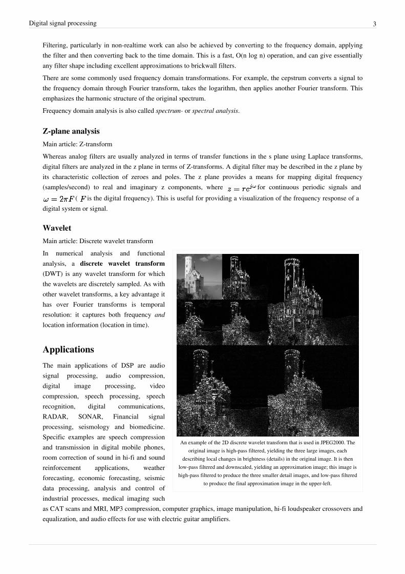
An example of the 2D discrete wavelet transform that is used in JPEG2000. Theoriginal image is high-pass filtered, yielding the three large images, each
describing local changes in brightness (details) in the original image. It is thenlow-pass filtered and downscaled, yielding an approximation image; this image ishigh-pass filtered to produce the three smaller detail images, and low-pass filtered
to produce the final approximation image in the upper-left.
In numerical analysis and functionalanalysis, a discrete wavelet transform(DWT) is any wavelet transform for whichthe wavelets are discretely sampled. As withother wavelet transforms, a key advantage ithas over Fourier transforms is temporalresolution: it captures both frequency andlocation information (location in time).
Applications
The main applications of DSP are audiosignal processing, audio compression,digital image processing, videocompression, speech processing, speechrecognition, digital communications,RADAR, SONAR, Financial signalprocessing, seismology and biomedicine.Specific examples are speech compressionand transmission in digital mobile phones,room correction of sound in hi-fi and soundreinforcement applications, weatherforecasting, economic forecasting, seismicdata processing, analysis and control ofindustrial processes, medical imaging suchas CAT scans and MRI, MP3 compression, computer graphics, image manipulation, hi-fi loudspeaker crossovers andequalization, and audio effects for use with electric guitar amplifiers.

Digital signal processing 4
ImplementationDepending on the requirements of the application, digital signal processing tasks can be implemented on generalpurpose computers (e.g. supercomputers, mainframe computers, or personal computers) or with embeddedprocessors that may or may not include specialized microprocessors called digital signal processors.Often when the processing requirement is not real-time, processing is economically done with an existinggeneral-purpose computer and the signal data (either input or output) exists in data files. This is essentially nodifferent from any other data processing, except DSP mathematical techniques (such as the FFT) are used, and thesampled data is usually assumed to be uniformly sampled in time or space. For example: processing digitalphotographs with software such as Photoshop.However, when the application requirement is real-time, DSP is often implemented using specializedmicroprocessors such as the DSP56000, the TMS320, or the SHARC. These often process data using fixed-pointarithmetic, though some more powerful versions use floating point arithmetic. For faster applications FPGAs mightbe used. Beginning in 2007, multicore implementations of DSPs have started to emerge from companies includingFreescale and Stream Processors, Inc. For faster applications with vast usage, ASICs might be designed specifically.For slow applications, a traditional slower processor such as a microcontroller may be adequate. Also a growingnumber of DSP applications are now being implemented on Embedded Systems using powerful PCs with aMulti-core processor.
Techniques•• Bilinear transform•• Discrete Fourier transform•• Discrete-time Fourier transform•• Filter design•• LTI system theory•• Minimum phase•• Transfer function•• Z-transform•• Goertzel algorithm•• s-plane
Related fields•• Analog signal processing•• Automatic control•• Computer Engineering•• Computer Science•• Data compression•• Dataflow programming•• Electrical engineering•• Fourier Analysis•• Information theory•• Machine Learning•• Real-time computing•• Stream processing•• Telecommunication•• Time series
Digital signal processing 5
•• Wavelet
References[1][1] Billings S.A. "Nonlinear System Identification: NARMAX Methods in the Time, Frequency, and Spatio-Temporal Domains". Wiley, 2013
Further reading• Alan V. Oppenheim, Ronald W. Schafer, John R. Buck : Discrete-Time Signal Processing, Prentice Hall, ISBN
0-13-754920-2• Boaz Porat: A Course in Digital Signal Processing, Wiley, ISBN 0-471-14961-6• Richard G. Lyons: Understanding Digital Signal Processing, Prentice Hall, ISBN 0-13-108989-7• Jonathan Yaakov Stein, Digital Signal Processing, a Computer Science Perspective, Wiley, ISBN 0-471-29546-9• Sen M. Kuo, Woon-Seng Gan: Digital Signal Processors: Architectures, Implementations, and Applications,
Prentice Hall, ISBN 0-13-035214-4• Bernard Mulgrew, Peter Grant, John Thompson: Digital Signal Processing - Concepts and Applications, Palgrave
Macmillan, ISBN 0-333-96356-3• Steven W. Smith (2002). Digital Signal Processing: A Practical Guide for Engineers and Scientists (http:/ / www.
dspguide. com). Newnes. ISBN 0-7506-7444-X.• Paul A. Lynn, Wolfgang Fuerst: Introductory Digital Signal Processing with Computer Applications, John Wiley
& Sons, ISBN 0-471-97984-8• James D. Broesch: Digital Signal Processing Demystified, Newnes, ISBN 1-878707-16-7• John G. Proakis, Dimitris Manolakis: Digital Signal Processing: Principles, Algorithms and Applications, 4th ed,
Pearson, April 2006, ISBN 978-0131873742• Hari Krishna Garg: Digital Signal Processing Algorithms, CRC Press, ISBN 0-8493-7178-3• P. Gaydecki: Foundations Of Digital Signal Processing: Theory, Algorithms And Hardware Design, Institution of
Electrical Engineers, ISBN 0-85296-431-5• Paul M. Embree, Damon Danieli: C++ Algorithms for Digital Signal Processing, Prentice Hall, ISBN
0-13-179144-3• Vijay Madisetti, Douglas B. Williams: The Digital Signal Processing Handbook, CRC Press, ISBN
0-8493-8572-5• Stergios Stergiopoulos: Advanced Signal Processing Handbook: Theory and Implementation for Radar, Sonar,
and Medical Imaging Real-Time Systems, CRC Press, ISBN 0-8493-3691-0• Joyce Van De Vegte: Fundamentals of Digital Signal Processing, Prentice Hall, ISBN 0-13-016077-6• Ashfaq Khan: Digital Signal Processing Fundamentals, Charles River Media, ISBN 1-58450-281-9• Jonathan M. Blackledge, Martin Turner: Digital Signal Processing: Mathematical and Computational Methods,
Software Development and Applications, Horwood Publishing, ISBN 1-898563-48-9• Doug Smith: Digital Signal Processing Technology: Essentials of the Communications Revolution, American
Radio Relay League, ISBN 0-87259-819-5• Charles A. Schuler: Digital Signal Processing: A Hands-On Approach, McGraw-Hill, ISBN 0-07-829744-3• James H. McClellan, Ronald W. Schafer, Mark A. Yoder: Signal Processing First, Prentice Hall, ISBN
0-13-090999-8• John G. Proakis: A Self-Study Guide for Digital Signal Processing, Prentice Hall, ISBN 0-13-143239-7• N. Ahmed and K.R. Rao (1975). Orthogonal Transforms for Digital Signal Processing. Springer-Verlag (Berlin –
Heidelberg – New York), ISBN 3-540-06556-3.
Discrete signal 6
Discrete signal
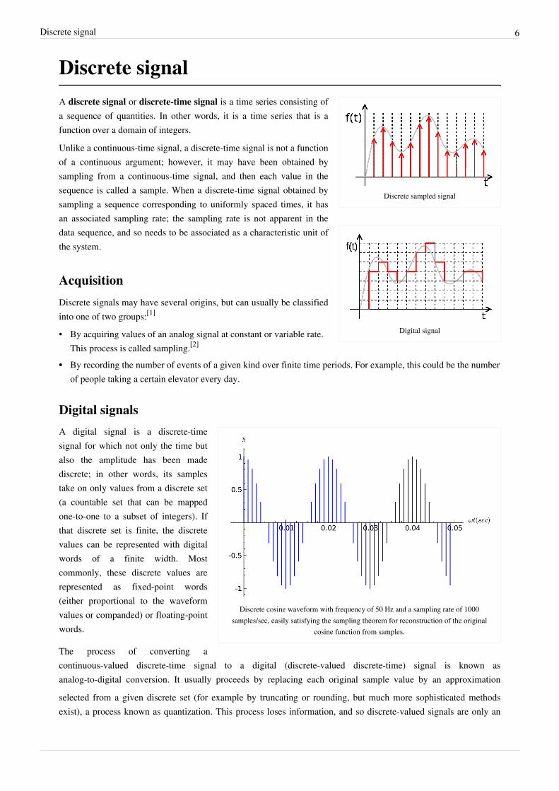
Discrete sampled signal
Digital signal
A discrete signal or discrete-time signal is a time series consisting ofa sequence of quantities. In other words, it is a time series that is afunction over a domain of integers.
Unlike a continuous-time signal, a discrete-time signal is not a functionof a continuous argument; however, it may have been obtained bysampling from a continuous-time signal, and then each value in thesequence is called a sample. When a discrete-time signal obtained bysampling a sequence corresponding to uniformly spaced times, it hasan associated sampling rate; the sampling rate is not apparent in thedata sequence, and so needs to be associated as a characteristic unit ofthe system.
Acquisition
Discrete signals may have several origins, but can usually be classifiedinto one of two groups:[1]
• By acquiring values of an analog signal at constant or variable rate.This process is called sampling.[2]
•• By recording the number of events of a given kind over finite time periods. For example, this could be the numberof people taking a certain elevator every day.
Digital signals
Discrete cosine waveform with frequency of 50 Hz and a sampling rate of 1000samples/sec, easily satisfying the sampling theorem for reconstruction of the original
cosine function from samples.
A digital signal is a discrete-timesignal for which not only the time butalso the amplitude has been madediscrete; in other words, its samplestake on only values from a discrete set(a countable set that can be mappedone-to-one to a subset of integers). Ifthat discrete set is finite, the discretevalues can be represented with digitalwords of a finite width. Mostcommonly, these discrete values arerepresented as fixed-point words(either proportional to the waveformvalues or companded) or floating-pointwords.
The process of converting acontinuous-valued discrete-time signal to a digital (discrete-valued discrete-time) signal is known asanalog-to-digital conversion. It usually proceeds by replacing each original sample value by an approximation
selected from a given discrete set (for example by truncating or rounding, but much more sophisticated methods exist), a process known as quantization. This process loses information, and so discrete-valued signals are only an
Discrete signal 7
approximation of the converted continuous-valued discrete-time signal, itself only an approximation of the originalcontinuous-valued continuous-time signal.Common practical digital signals are represented as 8-bit (256 levels), 16-bit (65,536 levels), 32-bit (4.3 billionlevels), and so on, though any number of quantization levels is possible, not just powers of two.
References[1][1] "Digital Signal Processing" Prentice Hall - Pages 11-12[2][2] "Digital Signal Processing: Instant access." Butterworth-Heinemann - Page 8
• Gershenfeld, Neil A. (1999). The Nature of mathematical Modeling. Cambridge University Press.ISBN 0-521-57095-6.
• Wagner, Thomas Charles Gordon (1959). Analytical transients. Wiley.
8
Sampling
Sampling (signal processing)
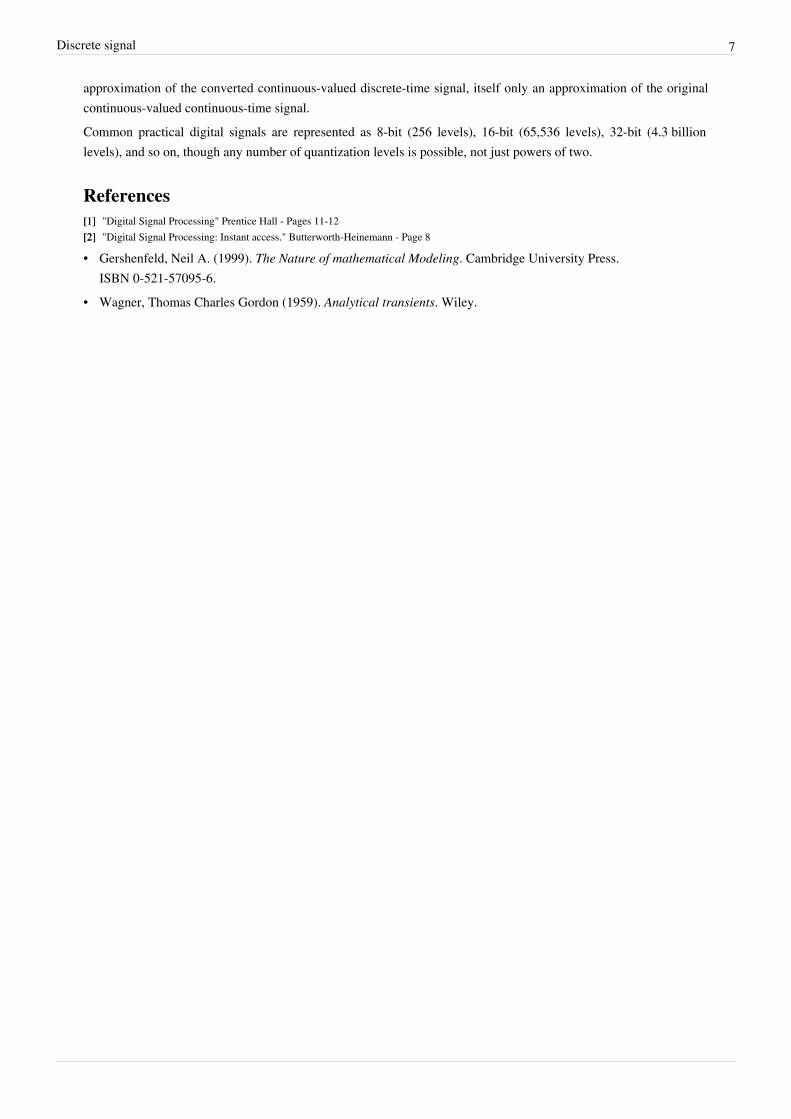
Signal sampling representation. The continuous signal is represented with a greencolored line while the discrete samples are indicated by the blue vertical lines.
In signal processing, sampling is thereduction of a continuous signal to a discretesignal. A common example is theconversion of a sound wave (a continuoussignal) to a sequence of samples (adiscrete-time signal).
A sample refers to a value or set of values ata point in time and/or space.
A sampler is a subsystem or operation thatextracts samples from a continuous signal.
A theoretical ideal sampler producessamples equivalent to the instantaneousvalue of the continuous signal at the desiredpoints.
Theory
See also: Nyquist–Shannon sampling theorem
Sampling can be done for functions varying in space, time, or any other dimension, and similar results are obtainedin two or more dimensions.For functions that vary with time, let s(t) be a continuous function (or "signal") to be sampled, and let sampling beperformed by measuring the value of the continuous function every T seconds, which is called the samplinginterval. Then the sampled function is given by the sequence:
s(nT), for integer values of n.The sampling frequency or sampling rate, f
s, is defined as the number of samples obtained in one second (samples
per second), thus fs
= 1/T.Reconstructing a continuous function from samples is done by interpolation algorithms. The Whittaker–Shannoninterpolation formula is mathematically equivalent to an ideal lowpass filter whose input is a sequence of Dirac deltafunctions that are modulated (multiplied) by the sample values. When the time interval between adjacent samples isa constant (T), the sequence of delta functions is called a Dirac comb. Mathematically, the modulated Dirac comb isequivalent to the product of the comb function with s(t). That purely mathematical abstraction is sometimes referredto as impulse sampling.Most sampled signals are not simply stored and reconstructed. But the fidelity of a theoretical reconstruction is acustomary measure of the effectiveness of sampling. That fidelity is reduced when s(t) contains frequencycomponents higher than f
s/2 Hz, which is known as the Nyquist frequency of the sampler. Therefore s(t) is usually
the output of a lowpass filter, functionally known as an anti-aliasing filter. Without an anti-aliasing filter,frequencies higher than the Nyquist frequency will influence the samples in a way that is misinterpreted by theinterpolation process.[1] For details, see Aliasing.

Sampling (signal processing) 9
Practical considerationsIn practice, the continuous signal is sampled using an analog-to-digital converter (ADC), a device with variousphysical limitations. This results in deviations from the theoretically perfect reconstruction, collectively referred toas distortion.Various types of distortion can occur, including:• Aliasing. Some amount of aliasing is inevitable because only theoretical, infinitely long, functions can have no
frequency content above the Nyquist frequency. Aliasing can be made arbitrarily small by using a sufficientlylarge order of the anti-aliasing filter.
• Aperture error results from the fact that the sample is obtained as a time average within a sampling region, ratherthan just being equal to the signal value at the sampling instant. In a capacitor-based sample and hold circuit,aperture error is introduced because the capacitor cannot instantly change voltage thus requiring the sample tohave non-zero width.
• Jitter or deviation from the precise sample timing intervals.• Noise, including thermal sensor noise, analog circuit noise, etc.• Slew rate limit error, caused by the inability of the ADC input value to change sufficiently rapidly.• Quantization as a consequence of the finite precision of words that represent the converted values.• Error due to other non-linear effects of the mapping of input voltage to converted output value (in addition to the
effects of quantization).Although the use of oversampling can completely eliminate aperture error and aliasing by shifting them out of thepass band, this technique cannot be practically used above a few GHz, and may be prohibitively expensive at muchlower frequencies. Furthermore, while oversampling can reduce quantization error and non-linearity, it cannoteliminate these entirely. Consequently, practical ADCs at audio frequencies typically do not exhibit aliasing,aperture error, and are not limited by quantization error. Instead, analog noise dominates. At RF and microwavefrequencies where oversampling is impractical and filters are expensive, aperture error, quantization error andaliasing can be significant limitations.Jitter, noise, and quantization are often analyzed by modeling them as random errors added to the sample values.Integration and zero-order hold effects can be analyzed as a form of low-pass filtering. The non-linearities of eitherADC or DAC are analyzed by replacing the ideal linear function mapping with a proposed nonlinear function.
Applications
Audio samplingDigital audio uses pulse-code modulation and digital signals for sound reproduction. This includes analog-to-digitalconversion (ADC), digital-to-analog conversion (DAC), storage, and transmission. In effect, the system commonlyreferred to as digital is in fact a discrete-time, discrete-level analog of a previous electrical analog. While modernsystems can be quite subtle in their methods, the primary usefulness of a digital system is the ability to store, retrieveand transmit signals without any loss of quality.
Sampling rate
When it is necessary to capture audio covering the entire 20–20,000 Hz range of human hearing, such as whenrecording music or many types of acoustic events, audio waveforms are typically sampled at 44.1 kHz (CD), 48 kHz(professional audio), 88.2 kHz, or 96 kHz. The approximately double-rate requirement is a consequence of theNyquist theorem. Sampling rates higher than about 50 kHz to 60 kHz cannot supply more usable information forhuman listeners. Early professional audio equipment manufacturers chose sampling rates in the region of 50 kHz forthis reason.
Sampling (signal processing) 10
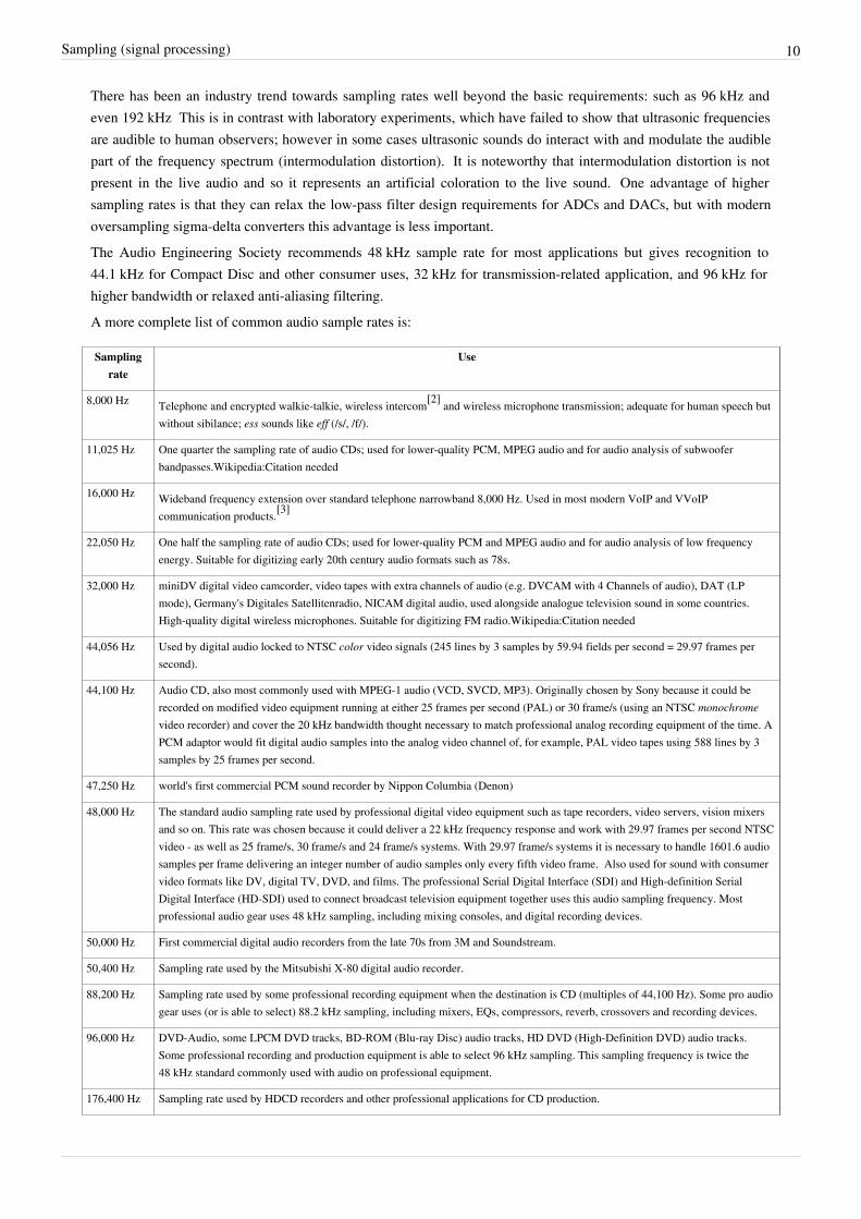
There has been an industry trend towards sampling rates well beyond the basic requirements: such as 96 kHz andeven 192 kHz This is in contrast with laboratory experiments, which have failed to show that ultrasonic frequenciesare audible to human observers; however in some cases ultrasonic sounds do interact with and modulate the audiblepart of the frequency spectrum (intermodulation distortion). It is noteworthy that intermodulation distortion is notpresent in the live audio and so it represents an artificial coloration to the live sound. One advantage of highersampling rates is that they can relax the low-pass filter design requirements for ADCs and DACs, but with modernoversampling sigma-delta converters this advantage is less important.The Audio Engineering Society recommends 48 kHz sample rate for most applications but gives recognition to44.1 kHz for Compact Disc and other consumer uses, 32 kHz for transmission-related application, and 96 kHz forhigher bandwidth or relaxed anti-aliasing filtering.A more complete list of common audio sample rates is:
Samplingrate
Use
8,000 Hz Telephone and encrypted walkie-talkie, wireless intercom[2] and wireless microphone transmission; adequate for human speech butwithout sibilance; ess sounds like eff (/s/, /f/).
11,025 Hz One quarter the sampling rate of audio CDs; used for lower-quality PCM, MPEG audio and for audio analysis of subwooferbandpasses.Wikipedia:Citation needed
16,000 Hz Wideband frequency extension over standard telephone narrowband 8,000 Hz. Used in most modern VoIP and VVoIPcommunication products.[3]
22,050 Hz One half the sampling rate of audio CDs; used for lower-quality PCM and MPEG audio and for audio analysis of low frequencyenergy. Suitable for digitizing early 20th century audio formats such as 78s.
32,000 Hz miniDV digital video camcorder, video tapes with extra channels of audio (e.g. DVCAM with 4 Channels of audio), DAT (LPmode), Germany's Digitales Satellitenradio, NICAM digital audio, used alongside analogue television sound in some countries.High-quality digital wireless microphones. Suitable for digitizing FM radio.Wikipedia:Citation needed
44,056 Hz Used by digital audio locked to NTSC color video signals (245 lines by 3 samples by 59.94 fields per second = 29.97 frames persecond).
44,100 Hz Audio CD, also most commonly used with MPEG-1 audio (VCD, SVCD, MP3). Originally chosen by Sony because it could berecorded on modified video equipment running at either 25 frames per second (PAL) or 30 frame/s (using an NTSC monochromevideo recorder) and cover the 20 kHz bandwidth thought necessary to match professional analog recording equipment of the time. APCM adaptor would fit digital audio samples into the analog video channel of, for example, PAL video tapes using 588 lines by 3samples by 25 frames per second.
47,250 Hz world's first commercial PCM sound recorder by Nippon Columbia (Denon)
48,000 Hz The standard audio sampling rate used by professional digital video equipment such as tape recorders, video servers, vision mixersand so on. This rate was chosen because it could deliver a 22 kHz frequency response and work with 29.97 frames per second NTSCvideo - as well as 25 frame/s, 30 frame/s and 24 frame/s systems. With 29.97 frame/s systems it is necessary to handle 1601.6 audiosamples per frame delivering an integer number of audio samples only every fifth video frame. Also used for sound with consumervideo formats like DV, digital TV, DVD, and films. The professional Serial Digital Interface (SDI) and High-definition SerialDigital Interface (HD-SDI) used to connect broadcast television equipment together uses this audio sampling frequency. Mostprofessional audio gear uses 48 kHz sampling, including mixing consoles, and digital recording devices.
50,000 Hz First commercial digital audio recorders from the late 70s from 3M and Soundstream.
50,400 Hz Sampling rate used by the Mitsubishi X-80 digital audio recorder.
88,200 Hz Sampling rate used by some professional recording equipment when the destination is CD (multiples of 44,100 Hz). Some pro audiogear uses (or is able to select) 88.2 kHz sampling, including mixers, EQs, compressors, reverb, crossovers and recording devices.
96,000 Hz DVD-Audio, some LPCM DVD tracks, BD-ROM (Blu-ray Disc) audio tracks, HD DVD (High-Definition DVD) audio tracks.Some professional recording and production equipment is able to select 96 kHz sampling. This sampling frequency is twice the48 kHz standard commonly used with audio on professional equipment.
176,400 Hz Sampling rate used by HDCD recorders and other professional applications for CD production.
Sampling (signal processing) 11
192,000 Hz DVD-Audio, some LPCM DVD tracks, BD-ROM (Blu-ray Disc) audio tracks, and HD DVD (High-Definition DVD) audio tracks,High-Definition audio recording devices and audio editing software. This sampling frequency is four times the 48 kHz standardcommonly used with audio on professional video equipment.
352,800 Hz Digital eXtreme Definition, used for recording and editing Super Audio CDs, as 1-bit DSD is not suited for editing. Eight times thefrequency of 44.1 kHz.
2,822,400 Hz SACD, 1-bit delta-sigma modulation process known as Direct Stream Digital, co-developed by Sony and Philips.
5,644,800 Hz Double-Rate DSD, 1-bit Direct Stream Digital at 2x the rate of the SACD. Used in some professional DSD recorders.
Bit depth
See also: Audio bit depthAudio is typically recorded at 8-, 16-, and 20-bit depth, which yield a theoretical maximumSignal-to-quantization-noise ratio (SQNR) for a pure sine wave of, approximately, 49.93 dB, 98.09 dB and122.17 dB. CD quality audio uses 16-bit samples. Thermal noise limits the true number of bits that can be used inquantization. Few analog systems have signal to noise ratios (SNR) exceeding 120 dB. However, digital signalprocessing operations can have very high dynamic range, consequently it is common to perform mixing andmastering operations at 32-bit precision and then convert to 16 or 24 bit for distribution.
Speech sampling
Speech signals, i.e., signals intended to carry only human speech, can usually be sampled at a much lower rate. Formost phonemes, almost all of the energy is contained in the 5Hz-4 kHz range, allowing a sampling rate of 8 kHz.This is the sampling rate used by nearly all telephony systems, which use the G.711 sampling and quantizationspecifications.
Video samplingStandard-definition television (SDTV) uses either 720 by 480 pixels (US NTSC 525-line) or 704 by 576 pixels (UKPAL 625-line) for the visible picture area.High-definition television (HDTV) uses 720p (progressive), 1080i (interlaced), and 1080p (progressive, also knownas Full-HD).In digital video, the temporal sampling rate is defined the frame rate – or rather the field rate – rather than thenotional pixel clock. The image sampling frequency is the repetition rate of the sensor integration period. Since theintegration period may be significantly shorter than the time between repetitions, the sampling frequency can bedifferent from the inverse of the sample time:• 50 Hz – PAL video• 60 / 1.001 Hz ~= 59.94 Hz – NTSC videoVideo digital-to-analog converters operate in the megahertz range (from ~3 MHz for low quality composite videoscalers in early games consoles, to 250 MHz or more for the highest-resolution VGA output).When analog video is converted to digital video, a different sampling process occurs, this time at the pixelfrequency, corresponding to a spatial sampling rate along scan lines. A common pixel sampling rate is:• 13.5 MHz – CCIR 601, D1 videoSpatial sampling in the other direction is determined by the spacing of scan lines in the raster. The sampling ratesand resolutions in both spatial directions can be measured in units of lines per picture height.Spatial aliasing of high-frequency luma or chroma video components shows up as a moiré pattern.
Sampling (signal processing) 12
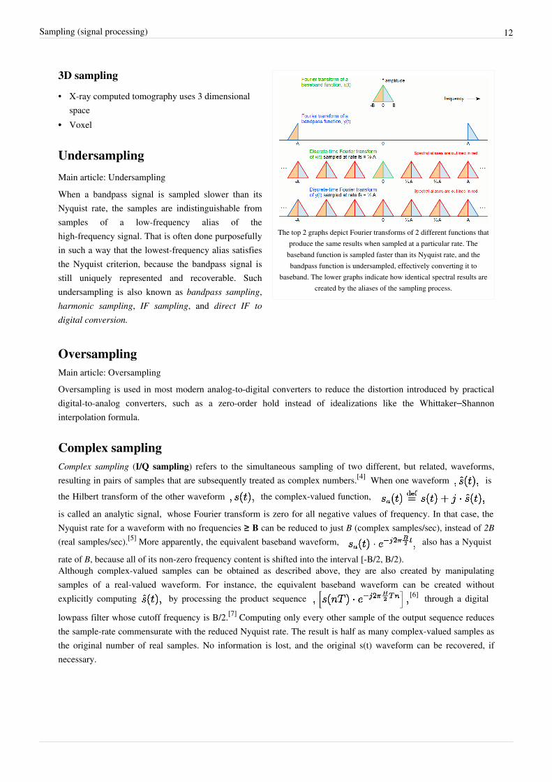
The top 2 graphs depict Fourier transforms of 2 different functions thatproduce the same results when sampled at a particular rate. The
baseband function is sampled faster than its Nyquist rate, and thebandpass function is undersampled, effectively converting it to
baseband. The lower graphs indicate how identical spectral results arecreated by the aliases of the sampling process.
3D sampling
• X-ray computed tomography uses 3 dimensionalspace
•• Voxel
Undersampling
Main article: UndersamplingWhen a bandpass signal is sampled slower than itsNyquist rate, the samples are indistinguishable fromsamples of a low-frequency alias of thehigh-frequency signal. That is often done purposefullyin such a way that the lowest-frequency alias satisfiesthe Nyquist criterion, because the bandpass signal isstill uniquely represented and recoverable. Suchundersampling is also known as bandpass sampling,harmonic sampling, IF sampling, and direct IF todigital conversion.
OversamplingMain article: OversamplingOversampling is used in most modern analog-to-digital converters to reduce the distortion introduced by practicaldigital-to-analog converters, such as a zero-order hold instead of idealizations like the Whittaker–Shannoninterpolation formula.
Complex samplingComplex sampling (I/Q sampling) refers to the simultaneous sampling of two different, but related, waveforms,resulting in pairs of samples that are subsequently treated as complex numbers.[4] When one waveform isthe Hilbert transform of the other waveform the complex-valued function,
is called an analytic signal, whose Fourier transform is zero for all negative values of frequency. In that case, theNyquist rate for a waveform with no frequencies ≥ B can be reduced to just B (complex samples/sec), instead of 2B(real samples/sec).[5] More apparently, the equivalent baseband waveform, also has a Nyquist
rate of B, because all of its non-zero frequency content is shifted into the interval [-B/2, B/2).Although complex-valued samples can be obtained as described above, they are also created by manipulatingsamples of a real-valued waveform. For instance, the equivalent baseband waveform can be created withoutexplicitly computing by processing the product sequence [6] through a digital
lowpass filter whose cutoff frequency is B/2.[7] Computing only every other sample of the output sequence reducesthe sample-rate commensurate with the reduced Nyquist rate. The result is half as many complex-valued samples asthe original number of real samples. No information is lost, and the original s(t) waveform can be recovered, ifnecessary.
Sampling (signal processing) 13
Notes[1] C. E. Shannon, "Communication in the presence of noise", Proc. Institute of Radio Engineers, vol. 37, no.1, pp. 10–21, Jan. 1949. Reprint as
classic paper in: Proc. IEEE, Vol. 86, No. 2, (Feb 1998) (http:/ / www. stanford. edu/ class/ ee104/ shannonpaper. pdf)[2] HME DX200 encrypted wireless intercom (http:/ / www. hme. com/ proDX200. cfm)[3] http:/ / www. voipsupply. com/ cisco-hd-voice[4] Sample-pairs are also sometimes viewed as points on a constellation diagram.[5] When the complex sample-rate is B, a frequency component at 0.6 B, for instance, will have an alias at −0.4 B, which is unambiguous
because of the constraint that the pre-sampled signal was analytic. Also see Aliasing#Complex_sinusoids[6][6] When s(t) is sampled at the Nyquist frequency (1/T = 2B), the product sequence simplifies to UNIQ-math-0-fdcc463dc40e329d-QINU[7][7] The sequence of complex numbers is convolved with the impulse response of a filter with real-valued coefficients. That is equivalent to
separately filtering the sequences of real parts and imaginary parts and reforming complex pairs at the outputs.
Citations
Further reading• Matt Pharr and Greg Humphreys, Physically Based Rendering: From Theory to Implementation, Morgan
Kaufmann, July 2004. ISBN 0-12-553180-X. The chapter on sampling ( available online (http:/ / graphics.stanford. edu/ ~mmp/ chapters/ pbrt_chapter7. pdf)) is nicely written with diagrams, core theory and code sample.
External links• Journal devoted to Sampling Theory (http:/ / www. stsip. org)• I/Q Data for Dummies (http:/ / whiteboard. ping. se/ SDR/ IQ) A page trying to answer the question Why I/Q
Data?
Sample and holdFor Neil Young song, see Trans (album). For remix album by Simian Mobile Disco, see Sample and Hold.
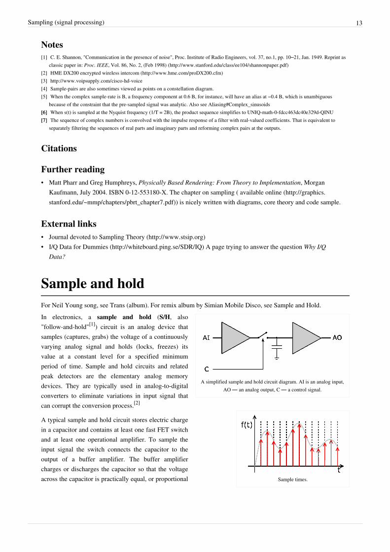
A simplified sample and hold circuit diagram. AI is an analog input,AO — an analog output, C — a control signal.
Sample times.
In electronics, a sample and hold (S/H, also"follow-and-hold"[1]) circuit is an analog device thatsamples (captures, grabs) the voltage of a continuouslyvarying analog signal and holds (locks, freezes) itsvalue at a constant level for a specified minimumperiod of time. Sample and hold circuits and relatedpeak detectors are the elementary analog memorydevices. They are typically used in analog-to-digitalconverters to eliminate variations in input signal thatcan corrupt the conversion process.[2]
A typical sample and hold circuit stores electric chargein a capacitor and contains at least one fast FET switchand at least one operational amplifier. To sample theinput signal the switch connects the capacitor to theoutput of a buffer amplifier. The buffer amplifiercharges or discharges the capacitor so that the voltageacross the capacitor is practically equal, or proportional

Sample and hold 14
Sample and hold.
to, input voltage. In hold mode the switch disconnects the capacitorfrom the buffer. The capacitor is invariably discharged by its ownleakage currents and useful load currents, which makes the circuitinherently volatile, but the loss of voltage (voltage drop) within aspecified hold time remains within an acceptable error margin.
For practically all commercial liquid crystal active matrix displaysbased on TN, IPS or VA electro-optic LC cells (excluding bi-stablephenomena), each pixel represents a small capacitor, which has to beperiodically charged to a level corresponding to the greyscale value(contrast) desired for a picture element. In order to maintain the level during a scanning cycle (frame period), anadditional electric capacitor is attached in parallel to each LC pixel to better hold the voltage. A thin-film FET switchis addressed to select a particular LC pixel and charge the picture information for it. In contrast to an S/H in generalelectronics, there is no output operational amplifier and no electrical signal AO. Instead, the charge on the holdcapacitors controls the deformation of the LC molecules and thereby the optical effect as its output. The invention ofthis concept and its implementation in thin-film technology have been honored with the IEEE Jun-ichi NishizawaMedal in 2011.[3]
During a scanning cycle, the picture doesn’t follow the input signal. This does not allow the eye to refresh and canlead to blurring during motion sequences, also the transition is visible between frames because the backlight isconstantly illuminated, adding to display motion blur.[4][5]
PurposeSample and hold circuits are used in linear systems. In some kinds of analog-to-digital converters, the input iscompared to a voltage generated internally from a digital-to-analog converter (DAC). The circuit tries a series ofvalues and stops converting once the voltages are equal, within some defined error margin. If the input value waspermitted to change during this comparison process, the resulting conversion would be inaccurate and possiblycompletely unrelated to the true input value. Such successive approximation converters will often incorporateinternal sample and hold circuitry. In addition, sample and hold circuits are often used when multiple samples needto be measured at the same time. Each value is sampled and held, using a common sample clock.
ImplementationTo keep the input voltage as stable as possible, it is essential that the capacitor have very low leakage, and that it notbe loaded to any significant degree which calls for a very high input impedance.
Notes[1][1] Horowitz and Hill, p. 220.[2][2] Kefauver and Patschke, p. 37.[3] Press release IEEE, Aug. 2011 (http:/ / www. ieee. org/ about/ news/ 2011/ honors_ceremony/ releases_nishizawa. html)[4] Charles Poynton is an authority on artifacts related to HDTV, and discusses motion artifacts succinctly and specifically (http:/ / www.
poynton. com/ PDFs/ Motion_portrayal. pdf)[5] Eye-tracking based motion blur on LCD (http:/ / ieeexplore. ieee. org/ xpls/ abs_all. jsp?arnumber=5583881& tag=1)

Sample and hold 15
References• Paul Horowitz, Winfield Hill (2001 ed.). The Art of Electronics (http:/ / books. google. com/
books?id=bkOMDgwFA28C& pg=PA220& dq=sample+ and+ hold& cd=1#v=onepage& q=sample and hold&f=false). Cambridge University Press. ISBN 0-521-37095-7.
• Alan P. Kefauver, David Patschke (2007). Fundamentals of digital audio (http:/ / books. google. com/books?id=UpzqCrj7QxYC& pg=PA60& dq=sample+ and+ hold& cd=7#v=onepage& q=sample and hold&f=false). A-R Editions, Inc. ISBN 0-89579-611-2.
• Analog Devices 21 page Tutorial "Sample and Hold Amplifiers" http:/ / www. analog. com/ static/ imported-files/tutorials/ MT-090. pdf
• Ndjountche, Tertulien (2011). CMOS Analog Integrated Circuits: High-Speed and Power-Efficient Design (http:// www. crcpress. com/ ecommerce_product/ product_detail. jsf?isbn=0& catno=k12557). Boca Raton, FL, USA:CRC Press. p. 925. ISBN 978-1-4398-5491-4.
• Applications of Monolithic Sample and hold Amplifiers-Intersil (http:/ / www. intersil. com/ data/ an/ an517. pdf)
Digital-to-analog converterFor digital television converter boxes, see digital television adapter.
8-channel digital-to-analog converter Cirrus LogicCS4382 as used in a soundcard.
In electronics, a digital-to-analog converter (DAC, D/A, D2A orD-to-A) is a function that converts digital data (usually binary)into an analog signal (current, voltage, or electric charge). Ananalog-to-digital converter (ADC) performs the reverse function.Unlike analog signals, digital data can be transmitted,manipulated, and stored without degradation, albeit with morecomplex equipment. But a DAC is needed to convert the digitalsignal to analog to drive an earphone or loudspeaker amplifier inorder to produce sound (analog air pressure waves).
DACs and their inverse, ADCs, are part of an enabling technologythat has contributed greatly to the digital revolution. To illustrate,consider a typical long-distance telephone call. The caller's voiceis converted into an analog electrical signal by a microphone, then the analog signal is converted to a digital streamby an ADC. The digital stream is then divided into packets where it may be mixed with other digital data, notnecessarily audio. The digital packets are then sent to the destination, but each packet may take a completelydifferent route and may not even arrive at the destination in the correct time order. The digital voice data is thenextracted from the packets and assembled into a digital data stream. A DAC converts this into an analog electricalsignal, which drives an audio amplifier, which in turn drives a loudspeaker, which finally produces sound.There are several DAC architectures; the suitability of a DAC for a particular application is determined by six mainparameters: physical size, power consumption, resolution, speed, accuracy, cost. Due to the complexity and the needfor precisely matched components, all but the most specialist DACs are implemented as integrated circuits (ICs).Digital-to-analog conversion can degrade a signal, so a DAC should be specified that that has insignificant errors interms of the application.DACs are commonly used in music players to convert digital data streams into analog audio signals. They are also used in televisions and mobile phones to convert digital video data into analog video signals which connect to the screen drivers to display monochrome or color images. These two applications use DACs at opposite ends of the speed/resolution trade-off. The audio DAC is a low speed high resolution type while the video DAC is a high speed low to medium resolution type. Discrete DACs would typically be extremely high speed low resolution power
Digital-to-analog converter 16
hungry types, as used in military radar systems. Very high speed test equipment, especially sampling oscilloscopes,may also use discrete DACS.
Overview
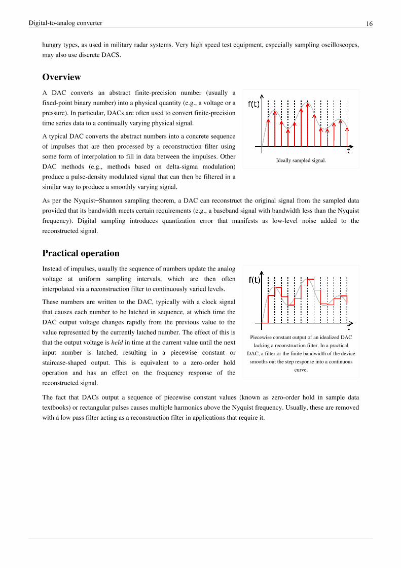
Ideally sampled signal.
A DAC converts an abstract finite-precision number (usually afixed-point binary number) into a physical quantity (e.g., a voltage or apressure). In particular, DACs are often used to convert finite-precisiontime series data to a continually varying physical signal.
A typical DAC converts the abstract numbers into a concrete sequenceof impulses that are then processed by a reconstruction filter usingsome form of interpolation to fill in data between the impulses. OtherDAC methods (e.g., methods based on delta-sigma modulation)produce a pulse-density modulated signal that can then be filtered in asimilar way to produce a smoothly varying signal.
As per the Nyquist–Shannon sampling theorem, a DAC can reconstruct the original signal from the sampled dataprovided that its bandwidth meets certain requirements (e.g., a baseband signal with bandwidth less than the Nyquistfrequency). Digital sampling introduces quantization error that manifests as low-level noise added to thereconstructed signal.
Practical operation
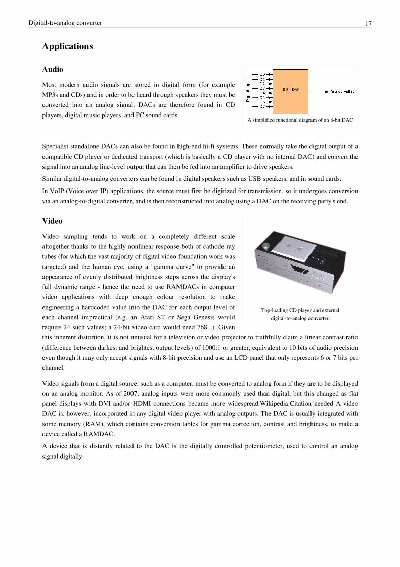
Piecewise constant output of an idealized DAClacking a reconstruction filter. In a practical
DAC, a filter or the finite bandwidth of the devicesmooths out the step response into a continuous
curve.
Instead of impulses, usually the sequence of numbers update the analogvoltage at uniform sampling intervals, which are then ofteninterpolated via a reconstruction filter to continuously varied levels.
These numbers are written to the DAC, typically with a clock signalthat causes each number to be latched in sequence, at which time theDAC output voltage changes rapidly from the previous value to thevalue represented by the currently latched number. The effect of this isthat the output voltage is held in time at the current value until the nextinput number is latched, resulting in a piecewise constant orstaircase-shaped output. This is equivalent to a zero-order holdoperation and has an effect on the frequency response of thereconstructed signal.
The fact that DACs output a sequence of piecewise constant values (known as zero-order hold in sample datatextbooks) or rectangular pulses causes multiple harmonics above the Nyquist frequency. Usually, these are removedwith a low pass filter acting as a reconstruction filter in applications that require it.
Digital-to-analog converter 17
Applications
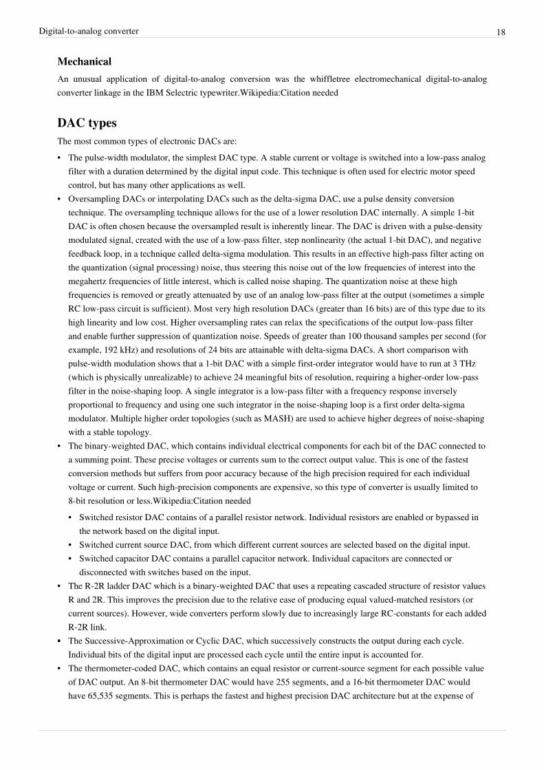
A simplified functional diagram of an 8-bit DAC
Audio
Most modern audio signals are stored in digital form (for exampleMP3s and CDs) and in order to be heard through speakers they must beconverted into an analog signal. DACs are therefore found in CDplayers, digital music players, and PC sound cards.
Specialist standalone DACs can also be found in high-end hi-fi systems. These normally take the digital output of acompatible CD player or dedicated transport (which is basically a CD player with no internal DAC) and convert thesignal into an analog line-level output that can then be fed into an amplifier to drive speakers.Similar digital-to-analog converters can be found in digital speakers such as USB speakers, and in sound cards.In VoIP (Voice over IP) applications, the source must first be digitized for transmission, so it undergoes conversionvia an analog-to-digital converter, and is then reconstructed into analog using a DAC on the receiving party's end.
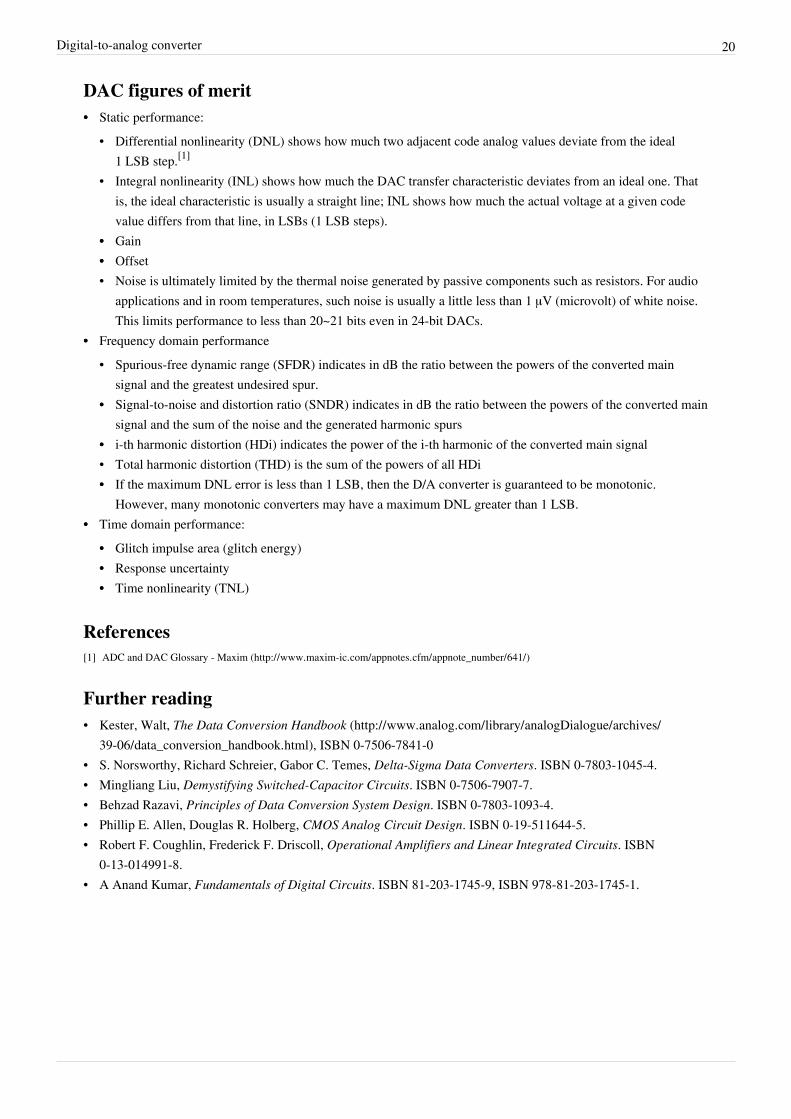
Top-loading CD player and externaldigital-to-analog converter.
Video
Video sampling tends to work on a completely different scalealtogether thanks to the highly nonlinear response both of cathode raytubes (for which the vast majority of digital video foundation work wastargeted) and the human eye, using a "gamma curve" to provide anappearance of evenly distributed brightness steps across the display'sfull dynamic range - hence the need to use RAMDACs in computervideo applications with deep enough colour resolution to makeengineering a hardcoded value into the DAC for each output level ofeach channel impractical (e.g. an Atari ST or Sega Genesis wouldrequire 24 such values; a 24-bit video card would need 768...). Giventhis inherent distortion, it is not unusual for a television or video projector to truthfully claim a linear contrast ratio(difference between darkest and brightest output levels) of 1000:1 or greater, equivalent to 10 bits of audio precisioneven though it may only accept signals with 8-bit precision and use an LCD panel that only represents 6 or 7 bits perchannel.
Video signals from a digital source, such as a computer, must be converted to analog form if they are to be displayedon an analog monitor. As of 2007, analog inputs were more commonly used than digital, but this changed as flatpanel displays with DVI and/or HDMI connections became more widespread.Wikipedia:Citation needed A videoDAC is, however, incorporated in any digital video player with analog outputs. The DAC is usually integrated withsome memory (RAM), which contains conversion tables for gamma correction, contrast and brightness, to make adevice called a RAMDAC.A device that is distantly related to the DAC is the digitally controlled potentiometer, used to control an analogsignal digitally.
Digital-to-analog converter 18
MechanicalAn unusual application of digital-to-analog conversion was the whiffletree electromechanical digital-to-analogconverter linkage in the IBM Selectric typewriter.Wikipedia:Citation needed
DAC typesThe most common types of electronic DACs are:• The pulse-width modulator, the simplest DAC type. A stable current or voltage is switched into a low-pass analog
filter with a duration determined by the digital input code. This technique is often used for electric motor speedcontrol, but has many other applications as well.
• Oversampling DACs or interpolating DACs such as the delta-sigma DAC, use a pulse density conversiontechnique. The oversampling technique allows for the use of a lower resolution DAC internally. A simple 1-bitDAC is often chosen because the oversampled result is inherently linear. The DAC is driven with a pulse-densitymodulated signal, created with the use of a low-pass filter, step nonlinearity (the actual 1-bit DAC), and negativefeedback loop, in a technique called delta-sigma modulation. This results in an effective high-pass filter acting onthe quantization (signal processing) noise, thus steering this noise out of the low frequencies of interest into themegahertz frequencies of little interest, which is called noise shaping. The quantization noise at these highfrequencies is removed or greatly attenuated by use of an analog low-pass filter at the output (sometimes a simpleRC low-pass circuit is sufficient). Most very high resolution DACs (greater than 16 bits) are of this type due to itshigh linearity and low cost. Higher oversampling rates can relax the specifications of the output low-pass filterand enable further suppression of quantization noise. Speeds of greater than 100 thousand samples per second (forexample, 192 kHz) and resolutions of 24 bits are attainable with delta-sigma DACs. A short comparison withpulse-width modulation shows that a 1-bit DAC with a simple first-order integrator would have to run at 3 THz(which is physically unrealizable) to achieve 24 meaningful bits of resolution, requiring a higher-order low-passfilter in the noise-shaping loop. A single integrator is a low-pass filter with a frequency response inverselyproportional to frequency and using one such integrator in the noise-shaping loop is a first order delta-sigmamodulator. Multiple higher order topologies (such as MASH) are used to achieve higher degrees of noise-shapingwith a stable topology.
• The binary-weighted DAC, which contains individual electrical components for each bit of the DAC connected toa summing point. These precise voltages or currents sum to the correct output value. This is one of the fastestconversion methods but suffers from poor accuracy because of the high precision required for each individualvoltage or current. Such high-precision components are expensive, so this type of converter is usually limited to8-bit resolution or less.Wikipedia:Citation needed• Switched resistor DAC contains of a parallel resistor network. Individual resistors are enabled or bypassed in
the network based on the digital input.• Switched current source DAC, from which different current sources are selected based on the digital input.• Switched capacitor DAC contains a parallel capacitor network. Individual capacitors are connected or
disconnected with switches based on the input.• The R-2R ladder DAC which is a binary-weighted DAC that uses a repeating cascaded structure of resistor values
R and 2R. This improves the precision due to the relative ease of producing equal valued-matched resistors (orcurrent sources). However, wide converters perform slowly due to increasingly large RC-constants for each addedR-2R link.
•• The Successive-Approximation or Cyclic DAC, which successively constructs the output during each cycle.Individual bits of the digital input are processed each cycle until the entire input is accounted for.
• The thermometer-coded DAC, which contains an equal resistor or current-source segment for each possible value of DAC output. An 8-bit thermometer DAC would have 255 segments, and a 16-bit thermometer DAC would have 65,535 segments. This is perhaps the fastest and highest precision DAC architecture but at the expense of

Digital-to-analog converter 19
high cost. Conversion speeds of >1 billion samples per second have been reached with this type of DAC.•• Hybrid DACs, which use a combination of the above techniques in a single converter. Most DAC integrated
circuits are of this type due to the difficulty of getting low cost, high speed and high precision in one device.•• The segmented DAC, which combines the thermometer-coded principle for the most significant bits and the
binary-weighted principle for the least significant bits. In this way, a compromise is obtained betweenprecision (by the use of the thermometer-coded principle) and number of resistors or current sources (by theuse of the binary-weighted principle). The full binary-weighted design means 0% segmentation, the fullthermometer-coded design means 100% segmentation.
• Most DACs, shown earlier in this list, rely on a constant reference voltage to create their output value.Alternatively, a multiplying DAC takes a variable input voltage for their conversion. This puts additional designconstraints on the bandwidth of the conversion circuit.
DAC performanceDACs are very important to system performance. The most important characteristics of these devices are:Resolution
The number of possible output levels the DAC is designed to reproduce. This is usually stated as the numberof bits it uses, which is the base two logarithm of the number of levels. For instance a 1 bit DAC is designed toreproduce 2 (21) levels while an 8 bit DAC is designed for 256 (28) levels. Resolution is related to the effectivenumber of bits which is a measurement of the actual resolution attained by the DAC. Resolution determinescolor depth in video applications and audio bit depth in audio applications.
Maximum sampling rateA measurement of the maximum speed at which the DACs circuitry can operate and still produce the correctoutput. As stated in the Nyquist–Shannon sampling theorem defines a relationship between the samplingfrequency and bandwidth of the sampled signal.
MonotonicityThe ability of a DAC's analog output to move only in the direction that the digital input moves (i.e., if theinput increases, the output doesn't dip before asserting the correct output.) This characteristic is very importantfor DACs used as a low frequency signal source or as a digitally programmable trim element.
Total harmonic distortion and noise (THD+N)A measurement of the distortion and noise introduced to the signal by the DAC. It is expressed as a percentageof the total power of unwanted harmonic distortion and noise that accompany the desired signal. This is a veryimportant DAC characteristic for dynamic and small signal DAC applications.
Dynamic rangeA measurement of the difference between the largest and smallest signals the DAC can reproduce expressed indecibels. This is usually related to resolution and noise floor.
Other measurements, such as phase distortion and jitter, can also be very important for some applications, some ofwhich (e.g. wireless data transmission, composite video) may even rely on accurate production of phase-adjustedsignals.Linear PCM audio sampling usually works on the basis of each bit of resolution being equivalent to 6 decibels ofamplitude (a 2x increase in volume or precision).Non-linear PCM encodings (A-law / μ-law, ADPCM, NICAM) attempt to improve their effective dynamic ranges bya variety of methods - logarithmic step sizes between the output signal strengths represented by each data bit (tradinggreater quantisation distortion of loud signals for better performance of quiet signals)
Digital-to-analog converter 20
DAC figures of merit•• Static performance:
• Differential nonlinearity (DNL) shows how much two adjacent code analog values deviate from the ideal1 LSB step.[1]
• Integral nonlinearity (INL) shows how much the DAC transfer characteristic deviates from an ideal one. Thatis, the ideal characteristic is usually a straight line; INL shows how much the actual voltage at a given codevalue differs from that line, in LSBs (1 LSB steps).
•• Gain•• Offset• Noise is ultimately limited by the thermal noise generated by passive components such as resistors. For audio
applications and in room temperatures, such noise is usually a little less than 1 μV (microvolt) of white noise.This limits performance to less than 20~21 bits even in 24-bit DACs.
•• Frequency domain performance• Spurious-free dynamic range (SFDR) indicates in dB the ratio between the powers of the converted main
signal and the greatest undesired spur.•• Signal-to-noise and distortion ratio (SNDR) indicates in dB the ratio between the powers of the converted main
signal and the sum of the noise and the generated harmonic spurs•• i-th harmonic distortion (HDi) indicates the power of the i-th harmonic of the converted main signal• Total harmonic distortion (THD) is the sum of the powers of all HDi•• If the maximum DNL error is less than 1 LSB, then the D/A converter is guaranteed to be monotonic.
However, many monotonic converters may have a maximum DNL greater than 1 LSB.•• Time domain performance:
•• Glitch impulse area (glitch energy)•• Response uncertainty•• Time nonlinearity (TNL)
References[1] ADC and DAC Glossary - Maxim (http:/ / www. maxim-ic. com/ appnotes. cfm/ appnote_number/ 641/ )
Further reading• Kester, Walt, The Data Conversion Handbook (http:/ / www. analog. com/ library/ analogDialogue/ archives/
39-06/ data_conversion_handbook. html), ISBN 0-7506-7841-0• S. Norsworthy, Richard Schreier, Gabor C. Temes, Delta-Sigma Data Converters. ISBN 0-7803-1045-4.• Mingliang Liu, Demystifying Switched-Capacitor Circuits. ISBN 0-7506-7907-7.• Behzad Razavi, Principles of Data Conversion System Design. ISBN 0-7803-1093-4.• Phillip E. Allen, Douglas R. Holberg, CMOS Analog Circuit Design. ISBN 0-19-511644-5.• Robert F. Coughlin, Frederick F. Driscoll, Operational Amplifiers and Linear Integrated Circuits. ISBN
0-13-014991-8.• A Anand Kumar, Fundamentals of Digital Circuits. ISBN 81-203-1745-9, ISBN 978-81-203-1745-1.
Digital-to-analog converter 21
External links• ADC and DAC Glossary (http:/ / www. maxim-ic. com/ appnotes. cfm/ an_pk/ 641/ CMP/ WP-36)
Analog-to-digital converter
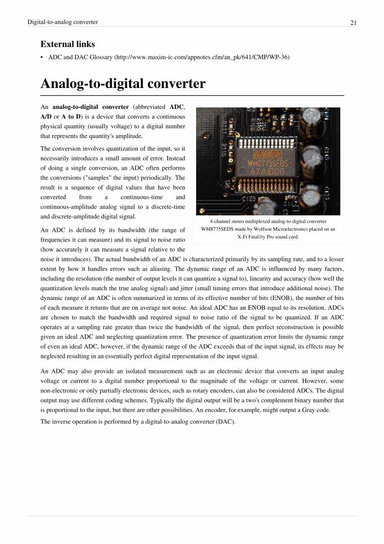
4-channel stereo multiplexed analog-to-digital converterWM8775SEDS made by Wolfson Microelectronics placed on an
X-Fi Fatal1ty Pro sound card.
An analog-to-digital converter (abbreviated ADC,A/D or A to D) is a device that converts a continuousphysical quantity (usually voltage) to a digital numberthat represents the quantity's amplitude.
The conversion involves quantization of the input, so itnecessarily introduces a small amount of error. Insteadof doing a single conversion, an ADC often performsthe conversions ("samples" the input) periodically. Theresult is a sequence of digital values that have beenconverted from a continuous-time andcontinuous-amplitude analog signal to a discrete-timeand discrete-amplitude digital signal.
An ADC is defined by its bandwidth (the range offrequencies it can measure) and its signal to noise ratio(how accurately it can measure a signal relative to thenoise it introduces). The actual bandwidth of an ADC is characterized primarily by its sampling rate, and to a lesserextent by how it handles errors such as aliasing. The dynamic range of an ADC is influenced by many factors,including the resolution (the number of output levels it can quantize a signal to), linearity and accuracy (how well thequantization levels match the true analog signal) and jitter (small timing errors that introduce additional noise). Thedynamic range of an ADC is often summarized in terms of its effective number of bits (ENOB), the number of bitsof each measure it returns that are on average not noise. An ideal ADC has an ENOB equal to its resolution. ADCsare chosen to match the bandwidth and required signal to noise ratio of the signal to be quantized. If an ADCoperates at a sampling rate greater than twice the bandwidth of the signal, then perfect reconstruction is possiblegiven an ideal ADC and neglecting quantization error. The presence of quantization error limits the dynamic rangeof even an ideal ADC, however, if the dynamic range of the ADC exceeds that of the input signal, its effects may beneglected resulting in an essentially perfect digital representation of the input signal.
An ADC may also provide an isolated measurement such as an electronic device that converts an input analogvoltage or current to a digital number proportional to the magnitude of the voltage or current. However, somenon-electronic or only partially electronic devices, such as rotary encoders, can also be considered ADCs. The digitaloutput may use different coding schemes. Typically the digital output will be a two's complement binary number thatis proportional to the input, but there are other possibilities. An encoder, for example, might output a Gray code.The inverse operation is performed by a digital-to-analog converter (DAC).
Analog-to-digital converter 22
Concepts
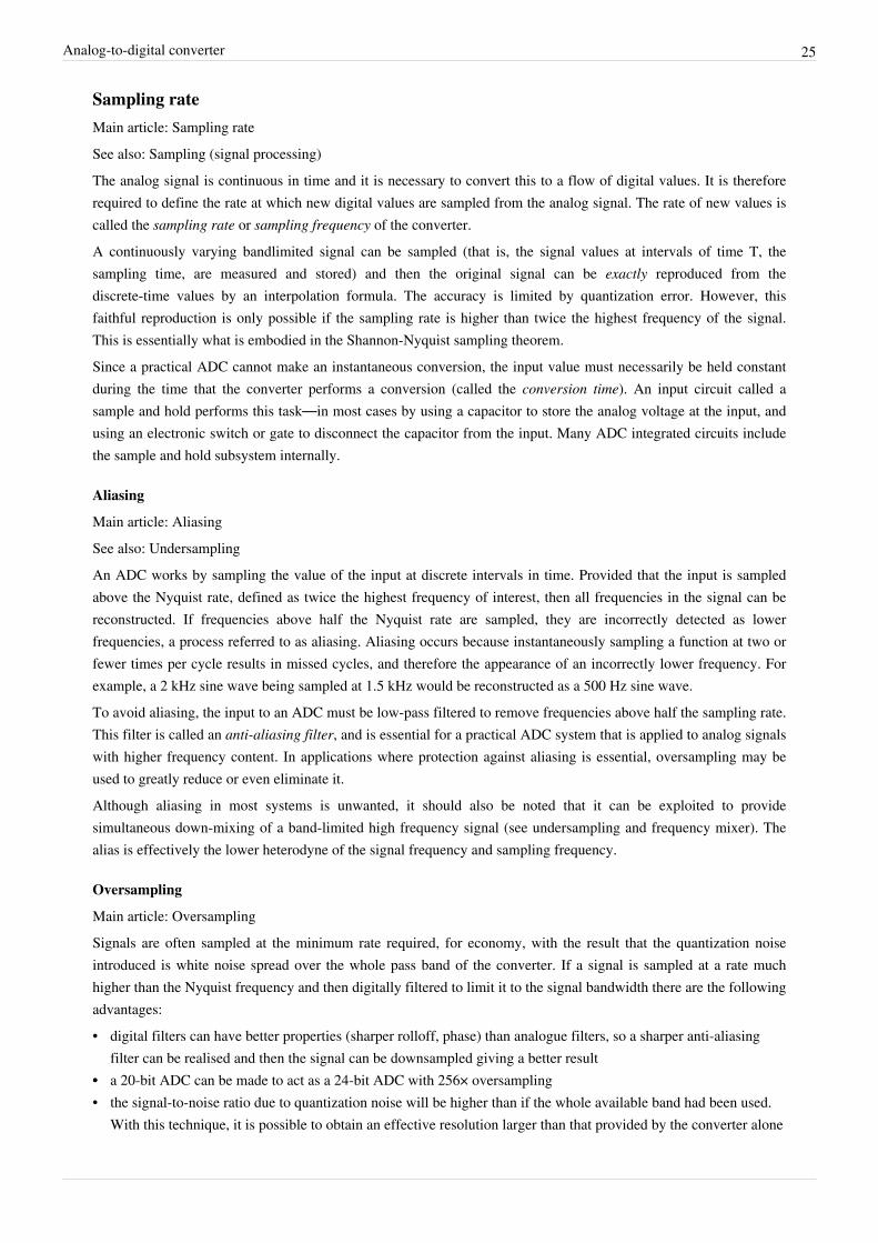
Resolution
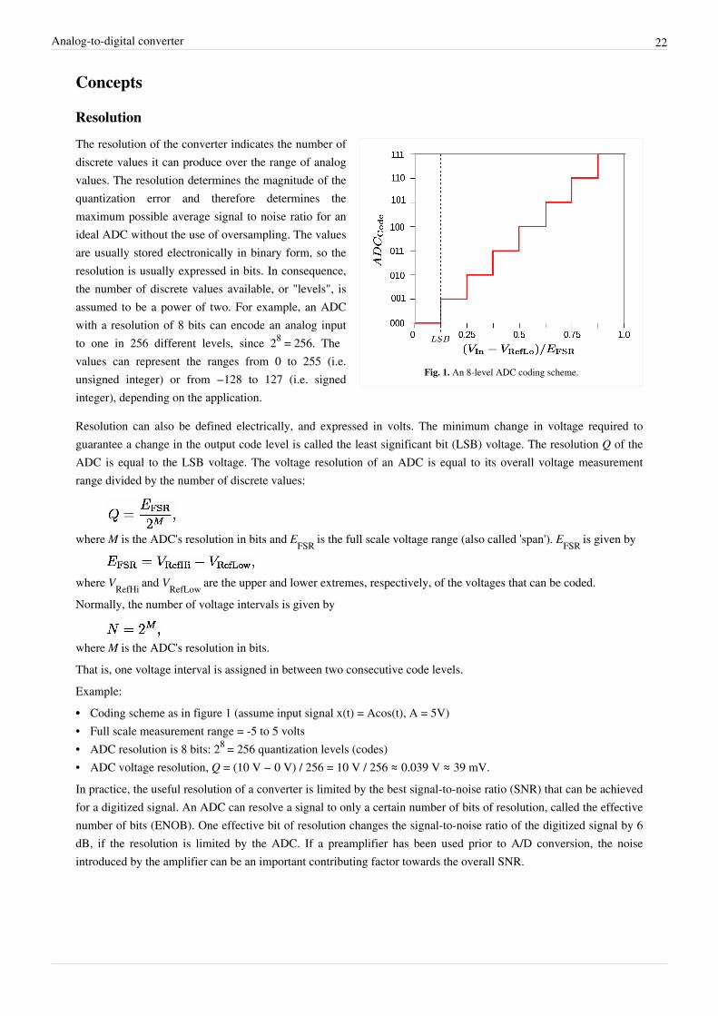
Fig. 1. An 8-level ADC coding scheme.
The resolution of the converter indicates the number ofdiscrete values it can produce over the range of analogvalues. The resolution determines the magnitude of thequantization error and therefore determines themaximum possible average signal to noise ratio for anideal ADC without the use of oversampling. The valuesare usually stored electronically in binary form, so theresolution is usually expressed in bits. In consequence,the number of discrete values available, or "levels", isassumed to be a power of two. For example, an ADCwith a resolution of 8 bits can encode an analog inputto one in 256 different levels, since 28 = 256. Thevalues can represent the ranges from 0 to 255 (i.e.unsigned integer) or from −128 to 127 (i.e. signedinteger), depending on the application.
Resolution can also be defined electrically, and expressed in volts. The minimum change in voltage required toguarantee a change in the output code level is called the least significant bit (LSB) voltage. The resolution Q of theADC is equal to the LSB voltage. The voltage resolution of an ADC is equal to its overall voltage measurementrange divided by the number of discrete values:
where M is the ADC's resolution in bits and EFSR is the full scale voltage range (also called 'span'). EFSR is given by
where VRefHi and VRefLow are the upper and lower extremes, respectively, of the voltages that can be coded.Normally, the number of voltage intervals is given by
where M is the ADC's resolution in bits.That is, one voltage interval is assigned in between two consecutive code levels.Example:•• Coding scheme as in figure 1 (assume input signal x(t) = Acos(t), A = 5V)• Full scale measurement range = -5 to 5 volts• ADC resolution is 8 bits: 28 = 256 quantization levels (codes)• ADC voltage resolution, Q = (10 V − 0 V) / 256 = 10 V / 256 ≈ 0.039 V ≈ 39 mV.In practice, the useful resolution of a converter is limited by the best signal-to-noise ratio (SNR) that can be achievedfor a digitized signal. An ADC can resolve a signal to only a certain number of bits of resolution, called the effectivenumber of bits (ENOB). One effective bit of resolution changes the signal-to-noise ratio of the digitized signal by 6dB, if the resolution is limited by the ADC. If a preamplifier has been used prior to A/D conversion, the noiseintroduced by the amplifier can be an important contributing factor towards the overall SNR.
Analog-to-digital converter 23
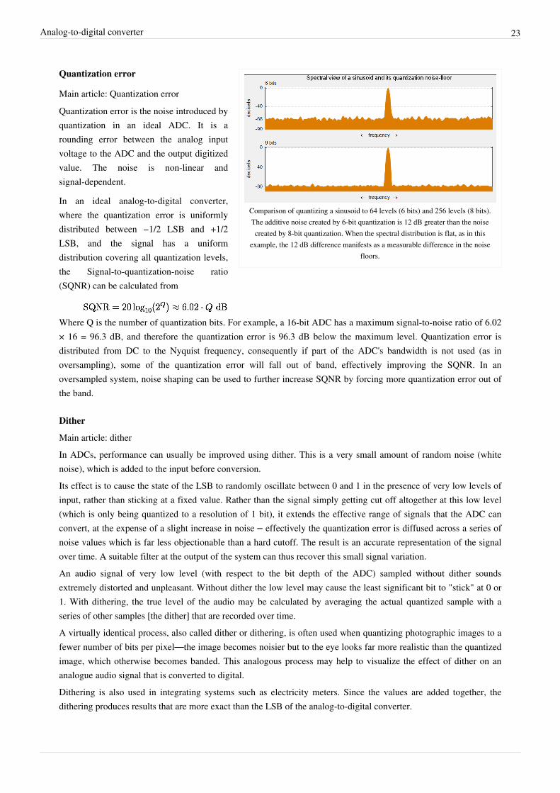
Comparison of quantizing a sinusoid to 64 levels (6 bits) and 256 levels (8 bits).The additive noise created by 6-bit quantization is 12 dB greater than the noisecreated by 8-bit quantization. When the spectral distribution is flat, as in this
example, the 12 dB difference manifests as a measurable difference in the noisefloors.
Quantization error
Main article: Quantization errorQuantization error is the noise introduced byquantization in an ideal ADC. It is arounding error between the analog inputvoltage to the ADC and the output digitizedvalue. The noise is non-linear andsignal-dependent.
In an ideal analog-to-digital converter,where the quantization error is uniformlydistributed between −1/2 LSB and +1/2LSB, and the signal has a uniformdistribution covering all quantization levels,the Signal-to-quantization-noise ratio(SQNR) can be calculated from
Where Q is the number of quantization bits. For example, a 16-bit ADC has a maximum signal-to-noise ratio of 6.02× 16 = 96.3 dB, and therefore the quantization error is 96.3 dB below the maximum level. Quantization error isdistributed from DC to the Nyquist frequency, consequently if part of the ADC's bandwidth is not used (as inoversampling), some of the quantization error will fall out of band, effectively improving the SQNR. In anoversampled system, noise shaping can be used to further increase SQNR by forcing more quantization error out ofthe band.
Dither
Main article: ditherIn ADCs, performance can usually be improved using dither. This is a very small amount of random noise (whitenoise), which is added to the input before conversion.Its effect is to cause the state of the LSB to randomly oscillate between 0 and 1 in the presence of very low levels ofinput, rather than sticking at a fixed value. Rather than the signal simply getting cut off altogether at this low level(which is only being quantized to a resolution of 1 bit), it extends the effective range of signals that the ADC canconvert, at the expense of a slight increase in noise – effectively the quantization error is diffused across a series ofnoise values which is far less objectionable than a hard cutoff. The result is an accurate representation of the signalover time. A suitable filter at the output of the system can thus recover this small signal variation.An audio signal of very low level (with respect to the bit depth of the ADC) sampled without dither soundsextremely distorted and unpleasant. Without dither the low level may cause the least significant bit to "stick" at 0 or1. With dithering, the true level of the audio may be calculated by averaging the actual quantized sample with aseries of other samples [the dither] that are recorded over time.A virtually identical process, also called dither or dithering, is often used when quantizing photographic images to afewer number of bits per pixel—the image becomes noisier but to the eye looks far more realistic than the quantizedimage, which otherwise becomes banded. This analogous process may help to visualize the effect of dither on ananalogue audio signal that is converted to digital.Dithering is also used in integrating systems such as electricity meters. Since the values are added together, thedithering produces results that are more exact than the LSB of the analog-to-digital converter.

Analog-to-digital converter 24
Note that dither can only increase the resolution of a sampler, it cannot improve the linearity, and thus accuracy doesnot necessarily improve.
AccuracyAn ADC has several sources of errors. Quantization error and (assuming the ADC is intended to be linear)non-linearity are intrinsic to any analog-to-digital conversion.These errors are measured in a unit called the least significant bit (LSB). In the above example of an eight-bit ADC,an error of one LSB is 1/256 of the full signal range, or about 0.4%.
Non-linearity
All ADCs suffer from non-linearity errors caused by their physical imperfections, causing their output to deviatefrom a linear function (or some other function, in the case of a deliberately non-linear ADC) of their input. Theseerrors can sometimes be mitigated by calibration, or prevented by testing.Important parameters for linearity are integral non-linearity (INL) and differential non-linearity (DNL). Thesenon-linearities reduce the dynamic range of the signals that can be digitized by the ADC, also reducing the effectiveresolution of the ADC.
Jitter
When digitizing a sine wave , the use of a non-ideal sampling clock will result in someuncertainty in when samples are recorded. Provided that the actual sampling time uncertainty due to the clock jitteris , the error caused by this phenomenon can be estimated as . This willresult in additional recorded noise that will reduce the effective number of bits (ENOB) below that predicted byquantization error alone.The error is zero for DC, small at low frequencies, but significant when high frequencies have high amplitudes. Thiseffect can be ignored if it is drowned out by the quantizing error. Jitter requirements can be calculated using the
following formula: , where q is the number of ADC bits.
Outputsize
(bits)
Signal Frequency
1 Hz 1 kHz 10 kHz 1 MHz 10 MHz 100 MHz 1 GHz
8 1,243 µs 1.24 µs 124 ns 1.24 ns 124 ps 12.4 ps 1.24 ps
10 311 µs 311 ns 31.1 ns 311 ps 31.1 ps 3.11 ps 0.31 ps
12 77.7 µs 77.7 ns 7.77 ns 77.7 ps 7.77 ps 0.78 ps 0.08 ps
14 19.4 µs 19.4 ns 1.94 ns 19.4 ps 1.94 ps 0.19 ps 0.02 ps
16 4.86 µs 4.86 ns 486 ps 4.86 ps 0.49 ps 0.05 ps –
18 1.21 ns 121 ps 6.32 ps 1.21 ps 0.12 ps – –
20 304 ps 30.4 ps 1.58 ps 0.16 ps – – –
Clock jitter is caused by phase noise.[1] The resolution of ADCs with a digitization bandwidth between 1 MHz and1 GHz is limited by jitter.When sampling audio signals at 44.1 kHz, the anti-aliasing filter should have eliminated all frequencies above22 kHz. The input frequency (in this case, < 22 kHz kHz), not the ADC clock frequency, is the determining factorwith respect to jitter performance.[2]
Analog-to-digital converter 25
Sampling rateMain article: Sampling rateSee also: Sampling (signal processing)The analog signal is continuous in time and it is necessary to convert this to a flow of digital values. It is thereforerequired to define the rate at which new digital values are sampled from the analog signal. The rate of new values iscalled the sampling rate or sampling frequency of the converter.A continuously varying bandlimited signal can be sampled (that is, the signal values at intervals of time T, thesampling time, are measured and stored) and then the original signal can be exactly reproduced from thediscrete-time values by an interpolation formula. The accuracy is limited by quantization error. However, thisfaithful reproduction is only possible if the sampling rate is higher than twice the highest frequency of the signal.This is essentially what is embodied in the Shannon-Nyquist sampling theorem.Since a practical ADC cannot make an instantaneous conversion, the input value must necessarily be held constantduring the time that the converter performs a conversion (called the conversion time). An input circuit called asample and hold performs this task—in most cases by using a capacitor to store the analog voltage at the input, andusing an electronic switch or gate to disconnect the capacitor from the input. Many ADC integrated circuits includethe sample and hold subsystem internally.
Aliasing
Main article: AliasingSee also: UndersamplingAn ADC works by sampling the value of the input at discrete intervals in time. Provided that the input is sampledabove the Nyquist rate, defined as twice the highest frequency of interest, then all frequencies in the signal can bereconstructed. If frequencies above half the Nyquist rate are sampled, they are incorrectly detected as lowerfrequencies, a process referred to as aliasing. Aliasing occurs because instantaneously sampling a function at two orfewer times per cycle results in missed cycles, and therefore the appearance of an incorrectly lower frequency. Forexample, a 2 kHz sine wave being sampled at 1.5 kHz would be reconstructed as a 500 Hz sine wave.To avoid aliasing, the input to an ADC must be low-pass filtered to remove frequencies above half the sampling rate.This filter is called an anti-aliasing filter, and is essential for a practical ADC system that is applied to analog signalswith higher frequency content. In applications where protection against aliasing is essential, oversampling may beused to greatly reduce or even eliminate it.Although aliasing in most systems is unwanted, it should also be noted that it can be exploited to providesimultaneous down-mixing of a band-limited high frequency signal (see undersampling and frequency mixer). Thealias is effectively the lower heterodyne of the signal frequency and sampling frequency.
Oversampling
Main article: OversamplingSignals are often sampled at the minimum rate required, for economy, with the result that the quantization noiseintroduced is white noise spread over the whole pass band of the converter. If a signal is sampled at a rate muchhigher than the Nyquist frequency and then digitally filtered to limit it to the signal bandwidth there are the followingadvantages:• digital filters can have better properties (sharper rolloff, phase) than analogue filters, so a sharper anti-aliasing
filter can be realised and then the signal can be downsampled giving a better result•• a 20-bit ADC can be made to act as a 24-bit ADC with 256× oversampling• the signal-to-noise ratio due to quantization noise will be higher than if the whole available band had been used.
With this technique, it is possible to obtain an effective resolution larger than that provided by the converter alone

Analog-to-digital converter 26
• The improvement in SNR is 3 dB (equivalent to 0.5 bits) per octave of oversampling which is not sufficient formany applications. Therefore, oversampling is usually coupled with noise shaping (see sigma-delta modulators).With noise shaping, the improvement is 6L+3 dB per octave where L is the order of loop filter used for noiseshaping. e.g. – a 2nd order loop filter will provide an improvement of 15 dB/octave.
Oversampling is typically used in audio frequency ADCs where the required sampling rate (typically 44.1 or48 kHz) is very low compared to the clock speed of typical transistor circuits (>1 MHz). In this case, by using theextra bandwidth to distribute quantization error onto out of band frequencies, the accuracy of the ADC can be greatlyincreased at no cost. Furthermore, as any aliased signals are also typically out of band, aliasing can often becompletely eliminated using very low cost filters.
Relative speed and precisionThe speed of an ADC varies by type. The Wilkinson ADC is limited by the clock rate which is processable bycurrent digital circuits. Currently,Wikipedia:Manual of Style/Dates and numbers#Chronological items frequenciesup to 300 MHz are possible.[3] For a successive-approximation ADC, the conversion time scales with the logarithmof the resolution, e.g. the number of bits. Thus for high resolution, it is possible that the successive-approximationADC is faster than the Wilkinson. However, the time consuming steps in the Wilkinson are digital, while those in thesuccessive-approximation are analog. Since analog is inherently slower than digital, as the resolution increases, thetime required also increases. Thus there are competing processes at work. Flash ADCs are certainly the fastest typeof the three. The conversion is basically performed in a single parallel step. For an 8-bit unit, conversion takes placein a few tens of nanoseconds.There is, as expected, somewhat of a tradeoff between speed and precision. Flash ADCs have drifts and uncertaintiesassociated with the comparator levels. This results in poor linearity. For successive-approximation ADCs, poorlinearity is also present, but less so than for flash ADCs. Here, non-linearity arises from accumulating errors from thesubtraction processes. Wilkinson ADCs have the highest linearity of the three. These have the best differentialnon-linearity. The other types require channel smoothing to achieve the level of the Wilkinson.
The sliding scale principleThe sliding scale or randomizing method can be employed to greatly improve the linearity of any type of ADC, butespecially flash and successive approximation types. For any ADC the mapping from input voltage to digital outputvalue is not exactly a floor or ceiling function as it should be. Under normal conditions, a pulse of a particularamplitude is always converted to a digital value. The problem lies in that the ranges of analog values for the digitizedvalues are not all of the same width, and the differential linearity decreases proportionally with the divergence fromthe average width. The sliding scale principle uses an averaging effect to overcome this phenomenon. A random, butknown analog voltage is added to the sampled input voltage. It is then converted to digital form, and the equivalentdigital amount is subtracted, thus restoring it to its original value. The advantage is that the conversion has takenplace at a random point. The statistical distribution of the final levels is decided by a weighted average over a regionof the range of the ADC. This in turn desensitizes it to the width of any specific level.
ADC typesThese are the most common ways of implementing an electronic ADC:• A direct-conversion ADC or flash ADC has a bank of comparators sampling the input signal in parallel, each
firing for their decoded voltage range. The comparator bank feeds a logic circuit that generates a code for each voltage range. Direct conversion is very fast, capable of gigahertz sampling rates, but usually has only 8 bits of resolution or fewer, since the number of comparators needed, 2N – 1, doubles with each additional bit, requiring a large, expensive circuit. ADCs of this type have a large die size, a high input capacitance, high power dissipation, and are prone to produce glitches at the output (by outputting an out-of-sequence code). Scaling to newer
Analog-to-digital converter 27
submicrometre technologies does not help as the device mismatch is the dominant design limitation. They areoften used for video, wideband communications or other fast signals in optical storage.
• A successive-approximation ADC uses a comparator to successively narrow a range that contains the inputvoltage. At each successive step, the converter compares the input voltage to the output of an internal digital toanalog converter which might represent the midpoint of a selected voltage range. At each step in this process, theapproximation is stored in a successive approximation register (SAR). For example, consider an input voltage of6.3 V and the initial range is 0 to 16 V. For the first step, the input 6.3 V is compared to 8 V (the midpoint of the0–16 V range). The comparator reports that the input voltage is less than 8 V, so the SAR is updated to narrow therange to 0–8 V. For the second step, the input voltage is compared to 4 V (midpoint of 0–8). The comparatorreports the input voltage is above 4 V, so the SAR is updated to reflect the input voltage is in the range 4–8 V. Forthe third step, the input voltage is compared with 6 V (halfway between 4 V and 8 V); the comparator reports theinput voltage is greater than 6 volts, and search range becomes 6–8 V. The steps are continued until the desiredresolution is reached.
• A ramp-compare ADC produces a saw-tooth signal that ramps up or down then quickly returns to zero. Whenthe ramp starts, a timer starts counting. When the ramp voltage matches the input, a comparator fires, and thetimer's value is recorded. Timed ramp converters require the least number of transistors. The ramp time issensitive to temperature because the circuit generating the ramp is often a simple oscillator. There are twosolutions: use a clocked counter driving a DAC and then use the comparator to preserve the counter's value, orcalibrate the timed ramp. A special advantage of the ramp-compare system is that comparing a second signal justrequires another comparator, and another register to store the voltage value. A very simple (non-linear)ramp-converter can be implemented with a microcontroller and one resistor and capacitor.[4] Vice versa, a filledcapacitor can be taken from an integrator, time-to-amplitude converter, phase detector, sample and hold circuit, orpeak and hold circuit and discharged. This has the advantage that a slow comparator cannot be disturbed by fastinput changes.
• The Wilkinson ADC was designed by D. H. Wilkinson in 1950. The Wilkinson ADC is based on the comparisonof an input voltage with that produced by a charging capacitor. The capacitor is allowed to charge until its voltageis equal to the amplitude of the input pulse (a comparator determines when this condition has been reached).Then, the capacitor is allowed to discharge linearly, which produces a ramp voltage. At the point when thecapacitor begins to discharge, a gate pulse is initiated. The gate pulse remains on until the capacitor is completelydischarged. Thus the duration of the gate pulse is directly proportional to the amplitude of the input pulse. Thisgate pulse operates a linear gate which receives pulses from a high-frequency oscillator clock. While the gate isopen, a discrete number of clock pulses pass through the linear gate and are counted by the address register. Thetime the linear gate is open is proportional to the amplitude of the input pulse, thus the number of clock pulsesrecorded in the address register is proportional also. Alternatively, the charging of the capacitor could bemonitored, rather than the discharge.
• An integrating ADC (also dual-slope or multi-slope ADC) applies the unknown input voltage to the input of anintegrator and allows the voltage to ramp for a fixed time period (the run-up period). Then a known referencevoltage of opposite polarity is applied to the integrator and is allowed to ramp until the integrator output returns tozero (the run-down period). The input voltage is computed as a function of the reference voltage, the constantrun-up time period, and the measured run-down time period. The run-down time measurement is usually made inunits of the converter's clock, so longer integration times allow for higher resolutions. Likewise, the speed of theconverter can be improved by sacrificing resolution. Converters of this type (or variations on the concept) areused in most digital voltmeters for their linearity and flexibility.
• A delta-encoded ADC or counter-ramp has an up-down counter that feeds a digital to analog converter (DAC). The input signal and the DAC both go to a comparator. The comparator controls the counter. The circuit uses negative feedback from the comparator to adjust the counter until the DAC's output is close enough to the input signal. The number is read from the counter. Delta converters have very wide ranges and high resolution, but the
Analog-to-digital converter 28
conversion time is dependent on the input signal level, though it will always have a guaranteed worst-case. Deltaconverters are often very good choices to read real-world signals. Most signals from physical systems do notchange abruptly. Some converters combine the delta and successive approximation approaches; this worksespecially well when high frequencies are known to be small in magnitude.
• A pipeline ADC (also called subranging quantizer) uses two or more steps of subranging. First, a coarseconversion is done. In a second step, the difference to the input signal is determined with a digital to analogconverter (DAC). This difference is then converted finer, and the results are combined in a last step. This can beconsidered a refinement of the successive-approximation ADC wherein the feedback reference signal consists ofthe interim conversion of a whole range of bits (for example, four bits) rather than just the next-most-significantbit. By combining the merits of the successive approximation and flash ADCs this type is fast, has a highresolution, and only requires a small die size.
• A sigma-delta ADC (also known as a delta-sigma ADC) oversamples the desired signal by a large factor andfilters the desired signal band. Generally, a smaller number of bits than required are converted using a Flash ADCafter the filter. The resulting signal, along with the error generated by the discrete levels of the Flash, is fed backand subtracted from the input to the filter. This negative feedback has the effect of noise shaping the error due tothe Flash so that it does not appear in the desired signal frequencies. A digital filter (decimation filter) follows theADC which reduces the sampling rate, filters off unwanted noise signal and increases the resolution of the output(sigma-delta modulation, also called delta-sigma modulation).
• A time-interleaved ADC uses M parallel ADCs where each ADC samples data every M:th cycle of the effectivesample clock. The result is that the sample rate is increased M times compared to what each individual ADC canmanage. In practice, the individual differences between the M ADCs degrade the overall performance reducingthe SFDR. However, technologies exist to correct for these time-interleaving mismatch errors.
• An ADC with intermediate FM stage first uses a voltage-to-frequency converter to convert the desired signalinto an oscillating signal with a frequency proportional to the voltage of the desired signal, and then uses afrequency counter to convert that frequency into a digital count proportional to the desired signal voltage. Longerintegration times allow for higher resolutions. Likewise, the speed of the converter can be improved by sacrificingresolution. The two parts of the ADC may be widely separated, with the frequency signal passed through anopto-isolator or transmitted wirelessly. Some such ADCs use sine wave or square wave frequency modulation;others use pulse-frequency modulation. Such ADCs were once the most popular way to show a digital display ofthe status of a remote analog sensor.[5][6][7][8][9]
There can be other ADCs that use a combination of electronics and other technologies:• A time-stretch analog-to-digital converter (TS-ADC) digitizes a very wide bandwidth analog signal, that
cannot be digitized by a conventional electronic ADC, by time-stretching the signal prior to digitization. Itcommonly uses a photonic preprocessor frontend to time-stretch the signal, which effectively slows the signaldown in time and compresses its bandwidth. As a result, an electronic backend ADC, that would have been tooslow to capture the original signal, can now capture this slowed down signal. For continuous capture of the signal,the frontend also divides the signal into multiple segments in addition to time-stretching. Each segment isindividually digitized by a separate electronic ADC. Finally, a digital signal processor rearranges the samples andremoves any distortions added by the frontend to yield the binary data that is the digital representation of theoriginal analog signal.
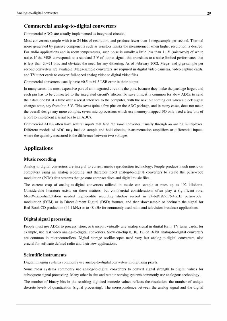
Analog-to-digital converter 29
Commercial analog-to-digital convertersCommercial ADCs are usually implemented as integrated circuits.Most converters sample with 6 to 24 bits of resolution, and produce fewer than 1 megasample per second. Thermalnoise generated by passive components such as resistors masks the measurement when higher resolution is desired.For audio applications and in room temperatures, such noise is usually a little less than 1 μV (microvolt) of whitenoise. If the MSB corresponds to a standard 2 V of output signal, this translates to a noise-limited performance thatis less than 20~21 bits, and obviates the need for any dithering. As of February 2002, Mega- and giga-sample persecond converters are available. Mega-sample converters are required in digital video cameras, video capture cards,and TV tuner cards to convert full-speed analog video to digital video files.Commercial converters usually have ±0.5 to ±1.5 LSB error in their output.In many cases, the most expensive part of an integrated circuit is the pins, because they make the package larger, andeach pin has to be connected to the integrated circuit's silicon. To save pins, it is common for slow ADCs to sendtheir data one bit at a time over a serial interface to the computer, with the next bit coming out when a clock signalchanges state, say from 0 to 5 V. This saves quite a few pins on the ADC package, and in many cases, does not makethe overall design any more complex (even microprocessors which use memory-mapped I/O only need a few bits ofa port to implement a serial bus to an ADC).Commercial ADCs often have several inputs that feed the same converter, usually through an analog multiplexer.Different models of ADC may include sample and hold circuits, instrumentation amplifiers or differential inputs,where the quantity measured is the difference between two voltages.
Applications
Music recordingAnalog-to-digital converters are integral to current music reproduction technology. People produce much music oncomputers using an analog recording and therefore need analog-to-digital converters to create the pulse-codemodulation (PCM) data streams that go onto compact discs and digital music files.The current crop of analog-to-digital converters utilized in music can sample at rates up to 192 kilohertz.Considerable literature exists on these matters, but commercial considerations often play a significant role.MostWikipedia:Citation needed high-profile recording studios record in 24-bit/192-176.4 kHz pulse-codemodulation (PCM) or in Direct Stream Digital (DSD) formats, and then downsample or decimate the signal forRed-Book CD production (44.1 kHz) or to 48 kHz for commonly used radio and television broadcast applications.
Digital signal processingPeople must use ADCs to process, store, or transport virtually any analog signal in digital form. TV tuner cards, forexample, use fast video analog-to-digital converters. Slow on-chip 8, 10, 12, or 16 bit analog-to-digital convertersare common in microcontrollers. Digital storage oscilloscopes need very fast analog-to-digital converters, alsocrucial for software defined radio and their new applications.
Scientific instrumentsDigital imaging systems commonly use analog-to-digital converters in digitizing pixels.Some radar systems commonly use analog-to-digital converters to convert signal strength to digital values forsubsequent signal processing. Many other in situ and remote sensing systems commonly use analogous technology.The number of binary bits in the resulting digitized numeric values reflects the resolution, the number of unique discrete levels of quantization (signal processing). The correspondence between the analog signal and the digital
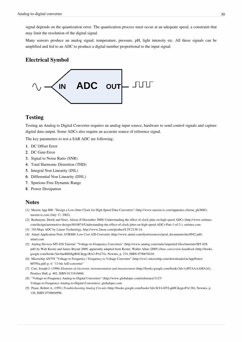
Analog-to-digital converter 30
signal depends on the quantization error. The quantization process must occur at an adequate speed, a constraint thatmay limit the resolution of the digital signal.Many sensors produce an analog signal; temperature, pressure, pH, light intensity etc. All these signals can beamplified and fed to an ADC to produce a digital number proportional to the input signal.
Electrical Symbol
TestingTesting an Analog to Digital Converter requires an analog input source, hardware to send control signals and capturedigital data output. Some ADCs also require an accurate source of reference signal.The key parameters to test a SAR ADC are following:1.1. DC Offset Error2.2. DC Gain Error3.3. Signal to Noise Ratio (SNR)4.4. Total Harmonic Distortion (THD)5.5. Integral Non Linearity (INL)6.6. Differential Non Linearity (DNL)7.7. Spurious Free Dynamic Range8.8. Power Dissipation
Notes[1] Maxim App 800: "Design a Low-Jitter Clock for High-Speed Data Converters" (http:/ / www. maxim-ic. com/ appnotes. cfm/ an_pk/ 800/ ).
maxim-ic.com (July 17, 2002).[2] Redmayne, Derek and Steer, Alison (8 December 2008) Understanding the effect of clock jitter on high-speed ADCs (http:/ / www. eetimes.
com/ design/ automotive-design/ 4010074/ Understanding-the-effect-of-clock-jitter-on-high-speed-ADCs-Part-1-of-2-). eetimes.com[3] 310 Msps ADC by Linear Technology, http:/ / www. linear. com/ product/ LTC2158-14.[4] Atmel Application Note AVR400: Low Cost A/D Converter (http:/ / www. atmel. com/ dyn/ resources/ prod_documents/ doc0942. pdf).
atmel.com[5] Analog Devices MT-028 Tutorial: "Voltage-to-Frequency Converters" (http:/ / www. analog. com/ static/ imported-files/ tutorials/ MT-028.
pdf) by Walt Kester and James Bryant 2009, apparently adapted from Kester, Walter Allan (2005) Data conversion handbook (http:/ / books.google. com/ books?id=0aeBS6SgtR4C& pg=RA2-PA274), Newnes, p. 274, ISBN 0750678410.
[6] Microchip AN795 "Voltage to Frequency / Frequency to Voltage Converter" (http:/ / ww1. microchip. com/ downloads/ en/ AppNotes/00795a. pdf) p. 4: "13-bit A/D converter"
[7] Carr, Joseph J. (1996) Elements of electronic instrumentation and measurement (http:/ / books. google. com/ books?id=1yBTAAAAMAAJ),Prentice Hall, p. 402, ISBN 0133416860.
[8] "Voltage-to-Frequency Analog-to-Digital Converters" (http:/ / www. globalspec. com/ reference/ 3127/Voltage-to-Frequency-Analog-to-Digital-Converters). globalspec.com
[9] Pease, Robert A. (1991) Troubleshooting Analog Circuits (http:/ / books. google. com/ books?id=3kY4-HYLqh0C& pg=PA130), Newnes, p.130, ISBN 0750694998.
Analog-to-digital converter 31
References• Knoll, Glenn F. (1989). Radiation Detection and Measurement (2nd ed.). New York: John Wiley & Sons.
ISBN 0471815047.• Nicholson, P. W. (1974). Nuclear Electronics. New York: John Wiley & Sons. pp. 315–316. ISBN 0471636975.
Further reading• Allen, Phillip E.; Holberg, Douglas R. CMOS Analog Circuit Design. ISBN 0-19-511644-5.• Fraden, Jacob (2010). Handbook of Modern Sensors: Physics, Designs, and Applications. Springer.
ISBN 978-1441964656.• Kester, Walt, ed. (2005). The Data Conversion Handbook (http:/ / www. analog. com/ library/ analogDialogue/
archives/ 39-06/ data_conversion_handbook. html). Elsevier: Newnes. ISBN 0-7506-7841-0.• Johns, David; Martin, Ken. Analog Integrated Circuit Design. ISBN 0-471-14448-7.• Liu, Mingliang. Demystifying Switched-Capacitor Circuits. ISBN 0-7506-7907-7.• Norsworthy, Steven R.; Schreier, Richard; Temes, Gabor C. (1997). Delta-Sigma Data Converters. IEEE Press.
ISBN 0-7803-1045-4.• Razavi, Behzad (1995). Principles of Data Conversion System Design. New York, NY: IEEE Press.
ISBN 0-7803-1093-4.• Staller, Len (February 24, 2005). "Understanding analog to digital converter specifications" (http:/ / www.
embedded. com/ design/ configurable-systems/ 4025078/Understanding-analog-to-digital-converter-specifications). Embedded Systems Design.
• Walden, R. H. (1999). "Analog-to-digital converter survey and analysis". IEEE Journal on Selected Areas inCommunications 17 (4): 539–550. doi: 10.1109/49.761034 (http:/ / dx. doi. org/ 10. 1109/ 49. 761034).
External links• Counting Type ADC (http:/ / ikalogic. com/ tut_adc. php) A simple tutorial showing how to build your first ADC.• An Introduction to Delta Sigma Converters (http:/ / www. beis. de/ Elektronik/ DeltaSigma/ DeltaSigma. html) A
very nice overview of Delta-Sigma converter theory.• Digital Dynamic Analysis of A/D Conversion Systems through Evaluation Software based on FFT/DFT Analysis
(http:/ / www. ieee. li/ pdf/ adc_evaluation_rf_expo_east_1987. pdf) RF Expo East, 1987• Which ADC Architecture Is Right for Your Application? (http:/ / www. analog. com/ library/ analogDialogue/
archives/ 39-06/ architecture. html) article by Walt Kester• ADC and DAC Glossary (http:/ / www. maxim-ic. com/ appnotes. cfm/ an_pk/ 641/ CMP/ ELK-11) Defines
commonly used technical terms.• Introduction to ADC in AVR (http:/ / www. robotplatform. com/ knowledge/ ADC/ adc_tutorial. html) – Analog
to digital conversion with Atmel microcontrollers• Signal processing and system aspects of time-interleaved ADCs. (http:/ / userver. ftw. at/ ~vogel/ TIADC. html)• Explanation of analog-digital converters with interactive principles of operations. (http:/ / www. onmyphd. com/
?p=analog. digital. converter)

Window function 32
Window functionFor the term used in SQL statements, see Window function (SQL)In signal processing, a window function (also known as an apodization function or tapering function) is amathematical function that is zero-valued outside of some chosen interval. For instance, a function that is constantinside the interval and zero elsewhere is called a rectangular window, which describes the shape of its graphicalrepresentation. When another function or waveform/data-sequence is multiplied by a window function, the product isalso zero-valued outside the interval: all that is left is the part where they overlap, the "view through the window".Applications of window functions include spectral analysis, filter design, and beamforming. In typical applications,the window functions used are non-negative smooth "bell-shaped" curves, though rectangle, triangle, and otherfunctions can be used.A more general definition of window functions does not require them to be identically zero outside an interval, aslong as the product of the window multiplied by its argument is square integrable, and, more specifically, that thefunction goes sufficiently rapidly toward zero.
ApplicationsApplications of window functions include spectral analysis and the design of finite impulse response filters.
Spectral analysisThe Fourier transform of the function cos ωt is zero, except at frequency ±ω. However, many other functions andwaveforms do not have convenient closed form transforms. Alternatively, one might be interested in their spectralcontent only during a certain time period.In either case, the Fourier transform (or something similar) can be applied on one or more finite intervals of thewaveform. In general, the transform is applied to the product of the waveform and a window function. Any window(including rectangular) affects the spectral estimate computed by this method.
Figure 1: Zoomed view of spectral leakage
Windowing
Windowing of a simple waveform likecos ωt causes its Fourier transform todevelop non-zero values (commonlycalled spectral leakage) at frequenciesother than ω. The leakage tends to beworst (highest) near ω and least atfrequencies farthest from ω.
If the waveform under analysiscomprises two sinusoids of differentfrequencies, leakage can interfere withthe ability to distinguish themspectrally. If their frequencies aredissimilar and one component isweaker, then leakage from the largercomponent can obscure the weaker
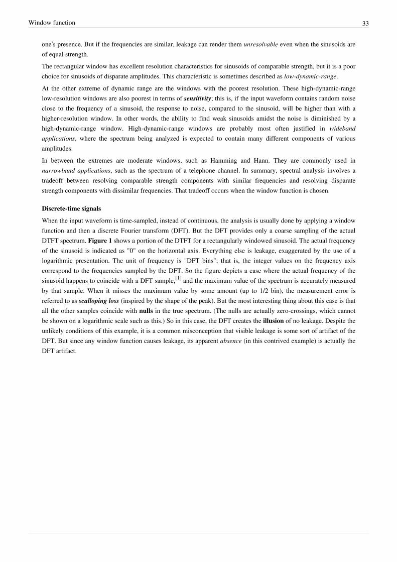
Window function 33
one’s presence. But if the frequencies are similar, leakage can render them unresolvable even when the sinusoids areof equal strength.The rectangular window has excellent resolution characteristics for sinusoids of comparable strength, but it is a poorchoice for sinusoids of disparate amplitudes. This characteristic is sometimes described as low-dynamic-range.At the other extreme of dynamic range are the windows with the poorest resolution. These high-dynamic-rangelow-resolution windows are also poorest in terms of sensitivity; this is, if the input waveform contains random noiseclose to the frequency of a sinusoid, the response to noise, compared to the sinusoid, will be higher than with ahigher-resolution window. In other words, the ability to find weak sinusoids amidst the noise is diminished by ahigh-dynamic-range window. High-dynamic-range windows are probably most often justified in widebandapplications, where the spectrum being analyzed is expected to contain many different components of variousamplitudes.In between the extremes are moderate windows, such as Hamming and Hann. They are commonly used innarrowband applications, such as the spectrum of a telephone channel. In summary, spectral analysis involves atradeoff between resolving comparable strength components with similar frequencies and resolving disparatestrength components with dissimilar frequencies. That tradeoff occurs when the window function is chosen.
Discrete-time signals
When the input waveform is time-sampled, instead of continuous, the analysis is usually done by applying a windowfunction and then a discrete Fourier transform (DFT). But the DFT provides only a coarse sampling of the actualDTFT spectrum. Figure 1 shows a portion of the DTFT for a rectangularly windowed sinusoid. The actual frequencyof the sinusoid is indicated as "0" on the horizontal axis. Everything else is leakage, exaggerated by the use of alogarithmic presentation. The unit of frequency is "DFT bins"; that is, the integer values on the frequency axiscorrespond to the frequencies sampled by the DFT. So the figure depicts a case where the actual frequency of thesinusoid happens to coincide with a DFT sample,[1] and the maximum value of the spectrum is accurately measuredby that sample. When it misses the maximum value by some amount (up to 1/2 bin), the measurement error isreferred to as scalloping loss (inspired by the shape of the peak). But the most interesting thing about this case is thatall the other samples coincide with nulls in the true spectrum. (The nulls are actually zero-crossings, which cannotbe shown on a logarithmic scale such as this.) So in this case, the DFT creates the illusion of no leakage. Despite theunlikely conditions of this example, it is a common misconception that visible leakage is some sort of artifact of theDFT. But since any window function causes leakage, its apparent absence (in this contrived example) is actually theDFT artifact.
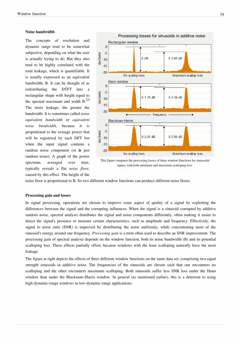
Window function 34
This figure compares the processing losses of three window functions for sinusoidalinputs, with both minimum and maximum scalloping loss.
Noise bandwidth
The concepts of resolution anddynamic range tend to be somewhatsubjective, depending on what the useris actually trying to do. But they alsotend to be highly correlated with thetotal leakage, which is quantifiable. Itis usually expressed as an equivalentbandwidth, B. It can be thought of asredistributing the DTFT into arectangular shape with height equal tothe spectral maximum and width B.[2]
The more leakage, the greater thebandwidth. It is sometimes called noiseequivalent bandwidth or equivalentnoise bandwidth, because it isproportional to the average power thatwill be registered by each DFT binwhen the input signal contains arandom noise component (or is justrandom noise). A graph of the powerspectrum, averaged over time,typically reveals a flat noise floor,caused by this effect. The height of thenoise floor is proportional to B. So two different window functions can produce different noise floors.
Processing gain and losses
In signal processing, operations are chosen to improve some aspect of quality of a signal by exploiting thedifferences between the signal and the corrupting influences. When the signal is a sinusoid corrupted by additiverandom noise, spectral analysis distributes the signal and noise components differently, often making it easier todetect the signal's presence or measure certain characteristics, such as amplitude and frequency. Effectively, thesignal to noise ratio (SNR) is improved by distributing the noise uniformly, while concentrating most of thesinusoid's energy around one frequency. Processing gain is a term often used to describe an SNR improvement. Theprocessing gain of spectral analysis depends on the window function, both its noise bandwidth (B) and its potentialscalloping loss. These effects partially offset, because windows with the least scalloping naturally have the mostleakage.The figure at right depicts the effects of three different window functions on the same data set, comprising two equalstrength sinusoids in additive noise. The frequencies of the sinusoids are chosen such that one encounters noscalloping and the other encounters maximum scalloping. Both sinusoids suffer less SNR loss under the Hannwindow than under the Blackman–Harris window. In general (as mentioned earlier), this is a deterrent to usinghigh-dynamic-range windows in low-dynamic-range applications.
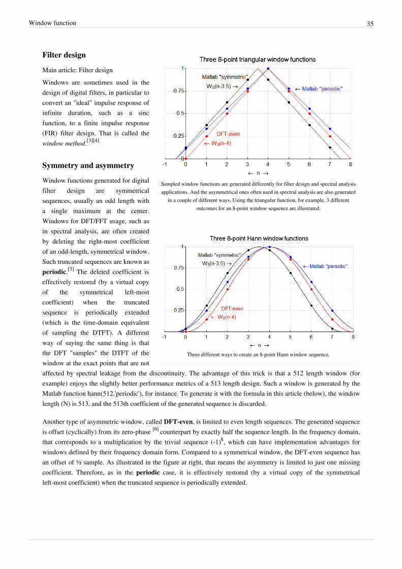
Window function 35
Sampled window functions are generated differently for filter design and spectral analysisapplications. And the asymmetrical ones often used in spectral analysis are also generated
in a couple of different ways. Using the triangular function, for example, 3 differentoutcomes for an 8-point window sequence are illustrated.
Three different ways to create an 8-point Hann window sequence.
Filter design
Main article: Filter designWindows are sometimes used in thedesign of digital filters, in particular toconvert an "ideal" impulse response ofinfinite duration, such as a sincfunction, to a finite impulse response(FIR) filter design. That is called thewindow method.[3][4]
Symmetry and asymmetry
Window functions generated for digitalfilter design are symmetricalsequences, usually an odd length witha single maximum at the center.Windows for DFT/FFT usage, such asin spectral analysis, are often createdby deleting the right-most coefficientof an odd-length, symmetrical window.Such truncated sequences are known asperiodic.[5] The deleted coefficient iseffectively restored (by a virtual copyof the symmetrical left-mostcoefficient) when the truncatedsequence is periodically extended(which is the time-domain equivalentof sampling the DTFT). A differentway of saying the same thing is thatthe DFT "samples" the DTFT of thewindow at the exact points that are notaffected by spectral leakage from the discontinuity. The advantage of this trick is that a 512 length window (forexample) enjoys the slightly better performance metrics of a 513 length design. Such a window is generated by theMatlab function hann(512,'periodic'), for instance. To generate it with the formula in this article (below), the windowlength (N) is 513, and the 513th coefficient of the generated sequence is discarded.
Another type of asymmetric window, called DFT-even, is limited to even length sequences. The generated sequenceis offset (cyclically) from its zero-phase [6] counterpart by exactly half the sequence length. In the frequency domain,that corresponds to a multiplication by the trivial sequence (-1)k, which can have implementation advantages forwindows defined by their frequency domain form. Compared to a symmetrical window, the DFT-even sequence hasan offset of ½ sample. As illustrated in the figure at right, that means the asymmetry is limited to just one missingcoefficient. Therefore, as in the periodic case, it is effectively restored (by a virtual copy of the symmetricalleft-most coefficient) when the truncated sequence is periodically extended.

Window function 36
Applications for which windows should not be usedIn some applications, it is preferable not to use a window function. For example:• In impact modal testing, when analyzing transient signals such as an excitation signal from hammer blow (see
Impulse excitation technique), where most of the energy is located at the beginning of the recording. Using anon-rectangular window would attenuate most of the energy and spread the frequency response unnecessarily.[7]
• A generalization of above, when measuring a self-windowing signal, such as an impulse, a shock response, a sineburst, a chirp burst, noise burst. Such signals are used in modal analysis. Applying a window function in this casewould just deteriorate the signal-to-noise ratio.
• When measuring a pseudo-random noise (PRN) excitation signal with period T, and using the same recordingperiod T. A PRN signal is periodic and therefore all spectral components of the signal will coincide with FFT bincenters with no leakage.[8]
• When measuring a repetitive signal locked-in to the sampling frequency, for example measuring the vibrationspectrum analysis during Shaft alignment, fault diagnosis of bearings, engines, gearboxes etc. Since the signal isrepetitive, all spectral energy is confined to multiples of the base repetition frequency.
• In an OFDM receiver, the input signal is directly multiplied by FFT without a window function. The frequencysub-carriers (aka symbols) are designed to align exactly to the FFT frequency bins. A cyclic prefix is usuallyadded to the transmitted signal, allowing frequency-selective fading due to multipath to be modeled as circularconvolution, thus avoiding intersymbol interference, which in OFDM is equivalent to spectral leakage.
A list of window functionsTerminology:
• N represents the width, in samples, of a discrete-time, symmetrical window function When N is an odd number, the non-flat windows have a singular maximum point.
When N is even, they have a double maximum.• It is sometimes useful to express as the lagged version of a sequence of samples of a zero-phase [6]
function:
• For instance, for even values of N we can describe the related DFT-even window as asdiscussed in the previous section. The DFT of such a sequence, in terms of the DFT of the sequence, is
• Each figure label includes the corresponding noise equivalent bandwidth metric (B), in units of DFT bins.
B-spline windowsB-spline windows can be obtained as k-fold convolutions of the rectangular window. They include the rectangularwindow itself (k = 1), the triangular window (k = 2) and the Parzen window (k = 4). Alternative definitions samplethe appropriate normalized B-spline basis functions instead of convolving discrete-time windows. A kth orderB-spline basis function is a piece-wise polynomial function of degree k−1 that is obtained by k-fold self-convolutionof the rectangular function.

Window function 37
Rectangular window
Rectangular window; B = 1.0000.
The rectangular window (sometimesknown as the boxcar or Dirichletwindow) is the simplest window,equivalent to replacing all but N valuesof a data sequence by zeros, making itappear as though the waveformsuddenly turns on and off:
Other windows are designed tomoderate these sudden changesbecause discontinuities haveundesirable effects on the discrete-timeFourier transform (DTFT) and/or the algorithms that produce samples of the DTFT.[9][10]
The rectangular window is the 1st order B-spline window as well as the 0th power cosine window.
Triangular window or equivalently the Bartlett window; B = 1.3333.
Triangular window
Triangular windows are given by:
where L can be N,[11] N+1, or N-1.[12]
The last one is also known as Bartlettwindow. All three definitions convergeat large N.
The triangular window is the 2nd orderB-spline window and can be seen asthe convolution of two half-sizedrectangular windows, giving it twice the width of the regular windows.
Parzen window
Parzen window; B = 1.92.
Not to be confused with Kernel densityestimation.
The Parzen window, also known as thede la Vallée Poussin window, is the4th order B-spline window.
Other polynomial windows

Window function 38
Welch window
Welch window; B = 1.20.
The Welch window consists of a singleparabolic section:
.
The defining quadratic polynomialreaches a value of zero at the samplesjust outside the span of the window.
Generalized Hammingwindows
Generalized Hamming windows are ofthe form:
.
They have only three non-zero DFT coefficients and share the benefits of a sparse frequency domain representationwith higher-order generalized cosine windows.
Hann (Hanning) window
Hann window; B = 1.5000.
Main article: Hann functionThe Hann window named after Juliusvon Hann and also known as theHanning (for being similar in nameand form to the Hamming window),von Hann and the raised cosinewindow is defined by:[13][14]
•• zero-phase version:
The ends of the cosine just touch zero, so the side-lobes roll off at about 18 dB per octave.[15]
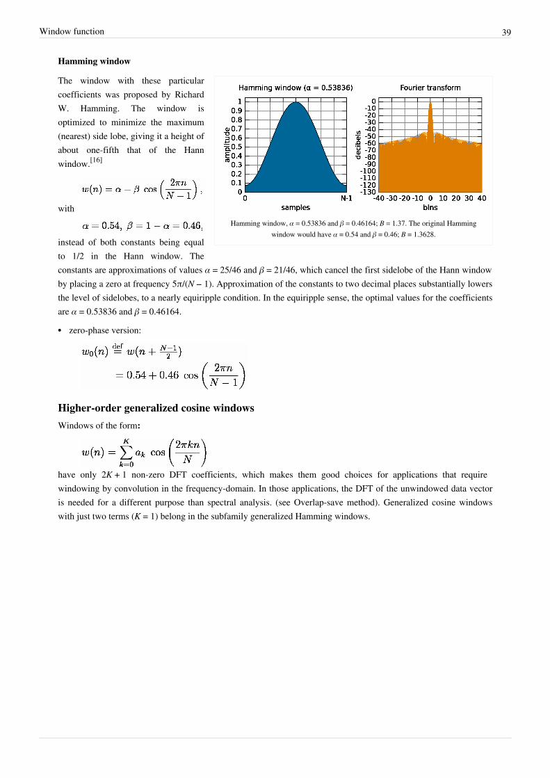
Window function 39
Hamming window
Hamming window, α = 0.53836 and β = 0.46164; B = 1.37. The original Hammingwindow would have α = 0.54 and β = 0.46; B = 1.3628.
The window with these particularcoefficients was proposed by RichardW. Hamming. The window isoptimized to minimize the maximum(nearest) side lobe, giving it a height ofabout one-fifth that of the Hannwindow.[16]
with
instead of both constants being equalto 1/2 in the Hann window. Theconstants are approximations of values α = 25/46 and β = 21/46, which cancel the first sidelobe of the Hann windowby placing a zero at frequency 5π/(N − 1). Approximation of the constants to two decimal places substantially lowersthe level of sidelobes, to a nearly equiripple condition. In the equiripple sense, the optimal values for the coefficientsare α = 0.53836 and β = 0.46164.
•• zero-phase version:
Higher-order generalized cosine windowsWindows of the form:
have only 2K + 1 non-zero DFT coefficients, which makes them good choices for applications that requirewindowing by convolution in the frequency-domain. In those applications, the DFT of the unwindowed data vectoris needed for a different purpose than spectral analysis. (see Overlap-save method). Generalized cosine windowswith just two terms (K = 1) belong in the subfamily generalized Hamming windows.
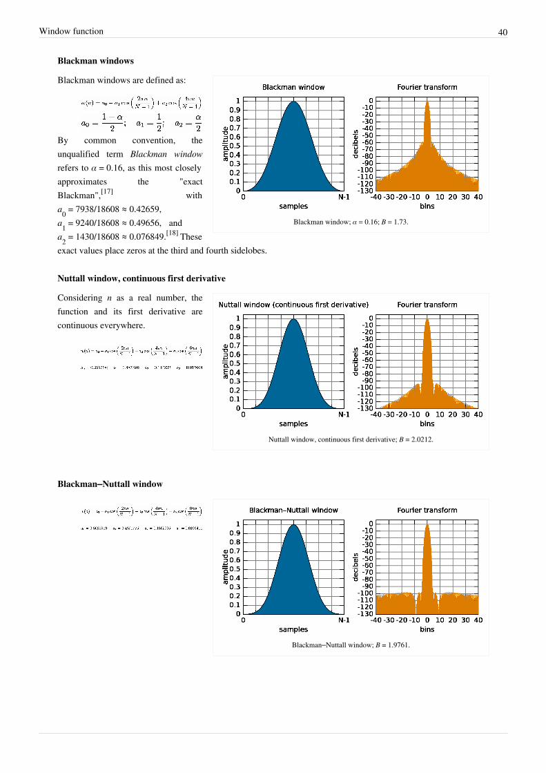
Window function 40
Blackman windows
Blackman window; α = 0.16; B = 1.73.
Blackman windows are defined as:
By common convention, theunqualified term Blackman windowrefers to α = 0.16, as this most closelyapproximates the "exactBlackman",[17] witha0 = 7938/18608 ≈ 0.42659,a1 = 9240/18608 ≈ 0.49656, anda2 = 1430/18608 ≈ 0.076849.[18] Theseexact values place zeros at the third and fourth sidelobes.
Nuttall window, continuous first derivative
Nuttall window, continuous first derivative; B = 2.0212.
Considering n as a real number, thefunction and its first derivative arecontinuous everywhere.
Blackman–Nuttall window
Blackman–Nuttall window; B = 1.9761.
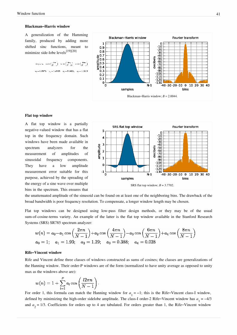
Window function 41
Blackman–Harris window
Blackman–Harris window; B = 2.0044.
A generalization of the Hammingfamily, produced by adding moreshifted sinc functions, meant tominimize side-lobe levels[19][20]
Flat top window
SRS flat top window; B = 3.7702.
A flat top window is a partiallynegative-valued window that has a flattop in the frequency domain. Suchwindows have been made available inspectrum analyzers for themeasurement of amplitudes ofsinusoidal frequency components.They have a low amplitudemeasurement error suitable for thispurpose, achieved by the spreading ofthe energy of a sine wave over multiplebins in the spectrum. This ensures thatthe unattenuated amplitude of the sinusoid can be found on at least one of the neighboring bins. The drawback of thebroad bandwidth is poor frequency resolution. To compensate, a longer window length may be chosen.
Flat top windows can be designed using low-pass filter design methods, or they may be of the usualsum-of-cosine-terms variety. An example of the latter is the flat top window available in the Stanford ResearchSystems (SRS) SR785 spectrum analyzer:
Rife–Vincent window
Rife and Vincent define three classes of windows constructed as sums of cosines; the classes are generalizations ofthe Hanning window. Their order-P windows are of the form (normalized to have unity average as opposed to unitymax as the windows above are):
.
For order 1, this formula can match the Hanning window for a1 = −1; this is the Rife–Vincent class-I window, defined by minimizing the high-order sidelobe amplitude. The class-I order-2 Rife–Vincent window has a1 = −4/3 and a2 = 1/3. Coefficients for orders up to 4 are tabulated. For orders greater than 1, the Rife–Vincent window
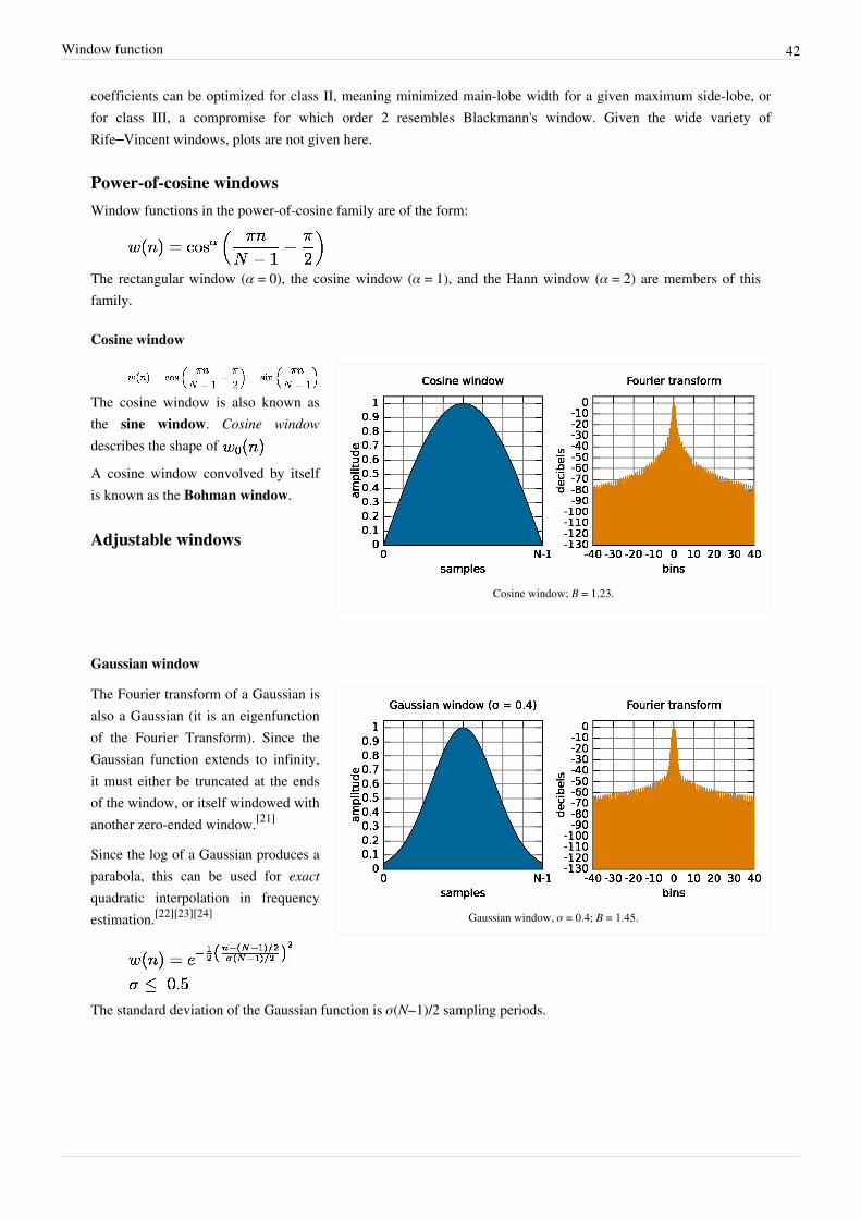
Window function 42
coefficients can be optimized for class II, meaning minimized main-lobe width for a given maximum side-lobe, orfor class III, a compromise for which order 2 resembles Blackmann's window. Given the wide variety ofRife–Vincent windows, plots are not given here.
Power-of-cosine windowsWindow functions in the power-of-cosine family are of the form:
The rectangular window (α = 0), the cosine window (α = 1), and the Hann window (α = 2) are members of thisfamily.
Cosine window
Cosine window; B = 1.23.
The cosine window is also known asthe sine window. Cosine windowdescribes the shape of
A cosine window convolved by itselfis known as the Bohman window.
Adjustable windows
Gaussian window
Gaussian window, σ = 0.4; B = 1.45.
The Fourier transform of a Gaussian isalso a Gaussian (it is an eigenfunctionof the Fourier Transform). Since theGaussian function extends to infinity,it must either be truncated at the endsof the window, or itself windowed withanother zero-ended window.[21]
Since the log of a Gaussian produces aparabola, this can be used for exactquadratic interpolation in frequencyestimation.[22][23][24]
The standard deviation of the Gaussian function is σ(N−1)/2 sampling periods.
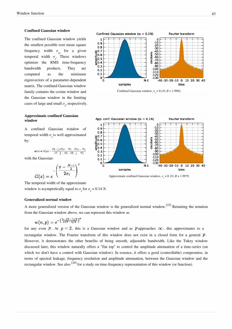
Window function 43
Confined Gaussian window, σt = 0.1N; B = 1.9982.
Confined Gaussian window
The confined Gaussian window yieldsthe smallest possible root mean squarefrequency width σω for a giventemporal width σt. These windowsoptimize the RMS time-frequencybandwidth products. They arecomputed as the minimumeigenvectors of a parameter-dependentmatrix. The confined Gaussian windowfamily contains the cosine window andthe Gaussian window in the limitingcases of large and small σt, respectively.
Approximate confined Gaussian window, σt = 0.1N; B = 1.9979.
Approximate confined Gaussianwindow
A confined Gaussian window oftemporal width σt is well approximatedby:
with the Gaussian:
The temporal width of the approximatewindow is asymptotically equal to σt for σt < 0.14 N.
Generalized normal window
A more generalized version of the Gaussian window is the generalized normal window.[25] Retaining the notationfrom the Gaussian window above, we can represent this window as
for any even . At , this is a Gaussian window and as approaches , this approximates to arectangular window. The Fourier transform of this window does not exist in a closed form for a general .However, it demonstrates the other benefits of being smooth, adjustable bandwidth. Like the Tukey windowdiscussed later, this window naturally offers a "flat top" to control the amplitude attenuation of a time-series (onwhich we don't have a control with Gaussian window). In essence, it offers a good (controllable) compromise, interms of spectral leakage, frequency resolution and amplitude attenuation, between the Gaussian window and therectangular window. See also [26] for a study on time-frequency representation of this window (or function).

Window function 44
Tukey window
Tukey window, α = 0.5; B = 1.22.
The Tukey window,[] also known asthe tapered cosine window, can beregarded as a cosine lobe of widthαN/2 that is convolved with arectangular window of width(1 − α/2)N.
At α = 0 it becomes rectangular, and at α = 1 it becomes a Hann window.
Planck-taper window
Planck-taper window, ε = 0.1; B = 1.10.
The so-called "Planck-taper" windowis a bump function that has beenwidely used in the theory of partitionsof unity in manifolds. It is a function everywhere, but is exactlyzero outside of a compact region,exactly one over an interval within thatregion, and varies smoothly andmonotonically between those limits. Itsuse as a window function in signalprocessing was first suggested in thecontext of gravitational-waveastronomy, inspired by the Planck distribution. It is defined as a piecewise function:
where
The amount of tapering (the region over which the function is exactly 1) is controlled by the parameter ε, withsmaller values giving sharper transitions.

Window function 45
DPSS or Slepian window
DPSS window, α = 2; B = 1.47.
DPSS window, α = 3; B = 1.77.
The DPSS (discrete prolate spheroidalsequence) or Slepian window is usedto maximize the energy concentrationin the main lobe.[27]
The main lobe ends at a bin given bythe parameter α.[28]
Kaiser window
Kaiser window, α = 2; B = 1.4963.
Main article: Kaiser windowThe Kaiser, or Kaiser-Bessel, windowis a simple approximation of the DPSSwindow using Bessel functions,discovered by Jim Kaiser.[29]
where I0 is the zero-th order modifiedBessel function of the first kind.Variable parameter α determines thetradeoff between main lobe width andside lobe levels of the spectral leakagepattern. The main lobe width, in between the nulls, is given by in units of DFT bins, and a typicalvalue of α is 3.
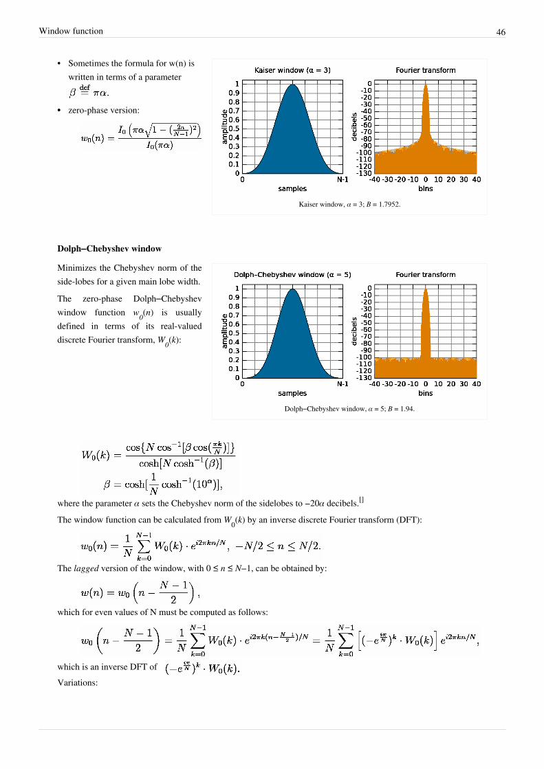
Window function 46
Kaiser window, α = 3; B = 1.7952.
• Sometimes the formula for w(n) iswritten in terms of a parameter
•• zero-phase version:
Dolph–Chebyshev window
Dolph–Chebyshev window, α = 5; B = 1.94.
Minimizes the Chebyshev norm of theside-lobes for a given main lobe width.
The zero-phase Dolph–Chebyshevwindow function w0(n) is usuallydefined in terms of its real-valueddiscrete Fourier transform, W0(k):
where the parameter α sets the Chebyshev norm of the sidelobes to −20α decibels.[]
The window function can be calculated from W0(k) by an inverse discrete Fourier transform (DFT):
The lagged version of the window, with 0 ≤ n ≤ N−1, can be obtained by:
which for even values of N must be computed as follows:
which is an inverse DFT of Variations:

Window function 47
• The DFT-even sequence (for even values of N) is given by which is the inverse DFT of
• Due to the equiripple condition, the time-domain window has discontinuities at the edges. An approximation thatavoids them, by allowing the equiripples to drop off at the edges, is a Taylor window [30].
• An alternative to the inverse DFT definition is also available.[31]. It isn't clear if it is the symmetric or DFT-even definition. But for typical values of N found in practice, the
difference is negligible.
Ultraspherical window
The Ultraspherical window's µ parameter determines whether its Fourier transform'sside-lobe amplitudes decrease, are level, or (shown here) increase with frequency.
The Ultraspherical window wasintroduced in 1984 by Roy Streit andhas application in antenna arraydesign, non-recursive filter design, andspectrum analysis.Like other adjustable windows, theUltraspherical window has parametersthat can be used to control its Fouriertransform main-lobe width and relativeside-lobe amplitude. Uncommon toother windows, it has an additionalparameter which can be used to set therate at which side-lobes decrease (orincrease) in amplitude.The window can be expressed in the time-domain as follows:
where is the Ultraspherical polynomial of degree N, and and control the side-lobe patterns.Certain specific values of yield other well-known windows: and give the Dolph–Chebyshev andSaramäki windows respectively. See here [32] for illustration of Ultraspherical windows with varied parametrization.
Exponential or Poisson window
Exponential window, τ = N/2, B = 1.08.
The Poisson window, or moregenerically the exponential windowincreases exponentially towards thecenter of the window and decreasesexponentially in the second half. Sincethe exponential function never reacheszero, the values of the window at itslimits are non-zero (it can be seen asthe multiplication of an exponentialfunction by a rectangular window ). Itis defined by
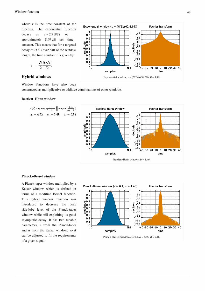
Window function 48
Exponential window, τ = (N/2)/(60/8.69), B = 3.46.
where τ is the time constant of thefunction. The exponential functiondecays as e ≃ 2.71828 orapproximately 8.69 dB per timeconstant. This means that for a targeteddecay of D dB over half of the windowlength, the time constant τ is given by
Hybrid windows
Window functions have also beenconstructed as multiplicative or additive combinations of other windows.
Bartlett–Hann window
Bartlett–Hann window; B = 1.46.
Planck–Bessel window
Planck–Bessel window, ε = 0.1, α = 4.45; B = 2.16.
A Planck-taper window multiplied by aKaiser window which is defined interms of a modified Bessel function.This hybrid window function wasintroduced to decrease the peakside-lobe level of the Planck-taperwindow while still exploiting its goodasymptotic decay. It has two tunableparameters, ε from the Planck-taperand α from the Kaiser window, so itcan be adjusted to fit the requirementsof a given signal.

Window function 49
Hann–Poisson window
Hann–Poisson window, α = 2; B = 2.02
A Hann window multiplied by aPoisson window, which has noside-lobes, in the sense that its Fouriertransform drops off forever away fromthe main lobe. It can thus be used inhill climbing algorithms like Newton'smethod.[33] The Hann–Poissonwindow is defined by:
where α is a parameter that controlsthe slope of the exponential.
Other windows
Lanczos window
Sinc or Lanczos window; B = 1.30.
• used in Lanczos resampling• for the Lanczos window, sinc(x) is
defined as sin(πx)/(πx)• also known as a sinc window,
because:
is
the main lobe of anormalized sinc function
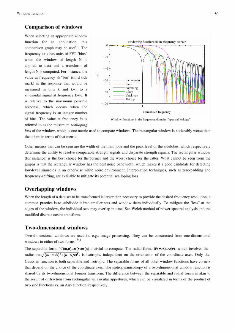
Window function 50
Comparison of windows
Window functions in the frequency domain ("spectral leakage")
When selecting an appropriate windowfunction for an application, thiscomparison graph may be useful. Thefrequency axis has units of FFT "bins"when the window of length N isapplied to data and a transform oflength N is computed. For instance, thevalue at frequency ½ "bin" (third tickmark) is the response that would bemeasured in bins k and k+1 to asinusoidal signal at frequency k+½. Itis relative to the maximum possibleresponse, which occurs when thesignal frequency is an integer numberof bins. The value at frequency ½ isreferred to as the maximum scallopingloss of the window, which is one metric used to compare windows. The rectangular window is noticeably worse thanthe others in terms of that metric.
Other metrics that can be seen are the width of the main lobe and the peak level of the sidelobes, which respectivelydetermine the ability to resolve comparable strength signals and disparate strength signals. The rectangular window(for instance) is the best choice for the former and the worst choice for the latter. What cannot be seen from thegraphs is that the rectangular window has the best noise bandwidth, which makes it a good candidate for detectinglow-level sinusoids in an otherwise white noise environment. Interpolation techniques, such as zero-padding andfrequency-shifting, are available to mitigate its potential scalloping loss.
Overlapping windowsWhen the length of a data set to be transformed is larger than necessary to provide the desired frequency resolution, acommon practice is to subdivide it into smaller sets and window them individually. To mitigate the "loss" at theedges of the window, the individual sets may overlap in time. See Welch method of power spectral analysis and themodified discrete cosine transform.
Two-dimensional windowsTwo-dimensional windows are used in, e.g., image processing. They can be constructed from one-dimensionalwindows in either of two forms.[34]
The separable form, is trivial to compute. The radial form, , which involves theradius , is isotropic, independent on the orientation of the coordinate axes. Only theGaussian function is both separable and isotropic. The separable forms of all other window functions have cornersthat depend on the choice of the coordinate axes. The isotropy/anisotropy of a two-dimensional window function isshared by its two-dimensional Fourier transform. The difference between the separable and radial forms is akin tothe result of diffraction from rectangular vs. circular appertures, which can be visualized in terms of the product oftwo sinc functions vs. an Airy function, respectively.
Window function 51
Notes[1][1] Another way of stating that condition is that the sinusoid happens to have an exact integer number of cycles within the length of the
rectangular window. The periodic repetition of such a segment contains no discontinuities.[2] Mathematically, the noise equivalent bandwidth of transfer function H is the bandwidth of an ideal rectangular filter with the same peak gain
as H that would pass the same power with white noise input. In the units of frequency f (e.g. hertz), it is given by:
UNIQ-math-0-fdcc463dc40e329d-QINU[3] http:/ / www. labbookpages. co. uk/ audio/ firWindowing. html[4] Mastering Windows: Improving Reconstruction (http:/ / www. cg. tuwien. ac. at/ research/ vis/ vismed/ Windows/ MasteringWindows. pdf)[5] http:/ / www. mathworks. com/ help/ signal/ ref/ hann. html[6] https:/ / ccrma. stanford. edu/ ~jos/ filters/ Zero_Phase_Filters_Even_Impulse. html[7] http:/ / www. hpmemory. org/ an/ pdf/ an_243. pdf The Fundamentals of Signal Analysis Application Note 243[8] http:/ / www. bksv. com/ doc/ bv0031. pdf Technical Review 1987-3 Use of Weighting Functions in DFT/FFT Analysis (Part I); Signals and
Units[9] https:/ / ccrma. stanford. edu/ ~jos/ sasp/ Properties. html[10] https:/ / ccrma. stanford. edu/ ~jos/ sasp/ Rectangular_window_properties. html[11] http:/ / www. mathworks. com/ help/ signal/ ref/ triang. html[12] https:/ / ccrma. stanford. edu/ ~jos/ sasp/ Bartlett_Triangular_Window. html[13] http:/ / www. mathworks. com/ help/ toolbox/ signal/ ref/ hann. html[14] http:/ / zone. ni. com/ reference/ en-XX/ help/ 371361E-01/ lvanls/ hanning_window/[15] https:/ / ccrma. stanford. edu/ ~jos/ sasp/ Hann_or_Hanning_or. html[16] https:/ / ccrma. stanford. edu/ ~jos/ sasp/ Hamming_Window. html[17] http:/ / mathworld. wolfram. com/ BlackmanFunction. html[18] http:/ / zone. ni. com/ reference/ en-XX/ help/ 371361E-01/ lvanlsconcepts/ char_smoothing_windows/ #Exact_Blackman[19] https:/ / ccrma. stanford. edu/ ~jos/ sasp/ Blackman_Harris_Window_Family. html[20] https:/ / ccrma. stanford. edu/ ~jos/ sasp/ Three_Term_Blackman_Harris_Window. html[21] https:/ / ccrma. stanford. edu/ ~jos/ sasp/ Gaussian_Window_Transform. html[22] https:/ / ccrma. stanford. edu/ ~jos/ sasp/ Matlab_Gaussian_Window. html[23] https:/ / ccrma. stanford. edu/ ~jos/ sasp/ Quadratic_Interpolation_Spectral_Peaks. html[24] https:/ / ccrma. stanford. edu/ ~jos/ sasp/ Gaussian_Window_Transform_I. html[25][25] Debejyo Chakraborty and Narayan Kovvali Generalized Normal Window for Digital Signal Processing in IEEE International Conference on
Acoustics, Speech and Signal Processing (ICASSP) 2013 6083 -- 6087 doi: 10.1109/ICASSP.2013.6638833[26][26] Diethorn, E.J., "The generalized exponential time-frequency distribution," Signal Processing, IEEE Transactions on , vol.42, no.5,
pp.1028,1037, May 1994 doi: 10.1109/78.295214[27] https:/ / ccrma. stanford. edu/ ~jos/ sasp/ Slepian_DPSS_Window. html[28] https:/ / ccrma. stanford. edu/ ~jos/ sasp/ Kaiser_DPSS_Windows_Compared. html[29] https:/ / ccrma. stanford. edu/ ~jos/ sasp/ Kaiser_Window. html[30] http:/ / www. mathworks. com/ help/ signal/ ref/ taylorwin. html[31] http:/ / practicalcryptography. com/ miscellaneous/ machine-learning/ implementing-dolph-chebyshev-window/[32] http:/ / octave. sourceforge. net/ signal/ function/ ultrwin. html[33] https:/ / ccrma. stanford. edu/ ~jos/ sasp/ Hann_Poisson_Window. html[34] Matt A. Bernstein, Kevin Franklin King, Xiaohong Joe Zhou (2007), Handbook of MRI Pulse Sequences, Elsevier; p.495-499. (http:/ /
books. google. com/ books?id=d6PLHcyejEIC& lpg=PA495& ots=tcBHi9Obfy& dq=image tapering tukey& pg=PA496#v=onepage& q&f=false)
Window function 52
References
Further reading• Nuttall, Albert H. (February 1981). "Some Windows with Very Good Sidelobe Behavior". IEEE Transactions on
Acoustics, Speech, and Signal Processing 29 (1): 84–91. doi: 10.1109/TASSP.1981.1163506 (http:/ / dx. doi. org/10. 1109/ TASSP. 1981. 1163506). Extends Harris' paper, covering all the window functions known at the time,along with key metric comparisons.
• Oppenheim, Alan V.; Schafer, Ronald W.; Buck, John A. (1999). Discrete-time signal processing. Upper SaddleRiver, N.J.: Prentice Hall. pp. 468–471. ISBN 0-13-754920-2.
• Bergen, S.W.A.; A. Antoniou (2004). "Design of Ultraspherical Window Functions with Prescribed SpectralCharacteristics". EURASIP Journal on Applied Signal Processing 2004 (13): 2053–2065. doi:10.1155/S1110865704403114 (http:/ / dx. doi. org/ 10. 1155/ S1110865704403114).
• Bergen, S.W.A.; A. Antoniou (2005). "Design of Nonrecursive Digital Filters Using the Ultraspherical WindowFunction". EURASIP Journal on Applied Signal Processing 2005 (12): 1910–1922. doi: 10.1155/ASP.2005.1910(http:/ / dx. doi. org/ 10. 1155/ ASP. 2005. 1910).
• US patent 7065150 (http:/ / worldwide. espacenet. com/ textdoc?DB=EPODOC& IDX=US7065150), Park,Young-Seo, "System and method for generating a root raised cosine orthogonal frequency division multiplexing(RRC OFDM) modulation", published 2003, issued 2006
• Albrecht, Hans-Helge (2012). Tailored minimum sidelobe and minimum sidelobe cosine-sum windows. A catalog.doi: 10.7795/110.20121022aa (http:/ / dx. doi. org/ 10. 7795/ 110. 20121022aa).
External links• LabView Help, Characteristics of Smoothing Filters, http:/ / zone. ni. com/ reference/ en-XX/ help/ 371361B-01/
lvanlsconcepts/ char_smoothing_windows/• Evaluation of Various Window Function using Multi-Instrument, http:/ / www. multi-instrument. com/ doc/
D1003/ Evaluation_of_Various_Window_Functions_using_Multi-Instrument_D1003. pdf
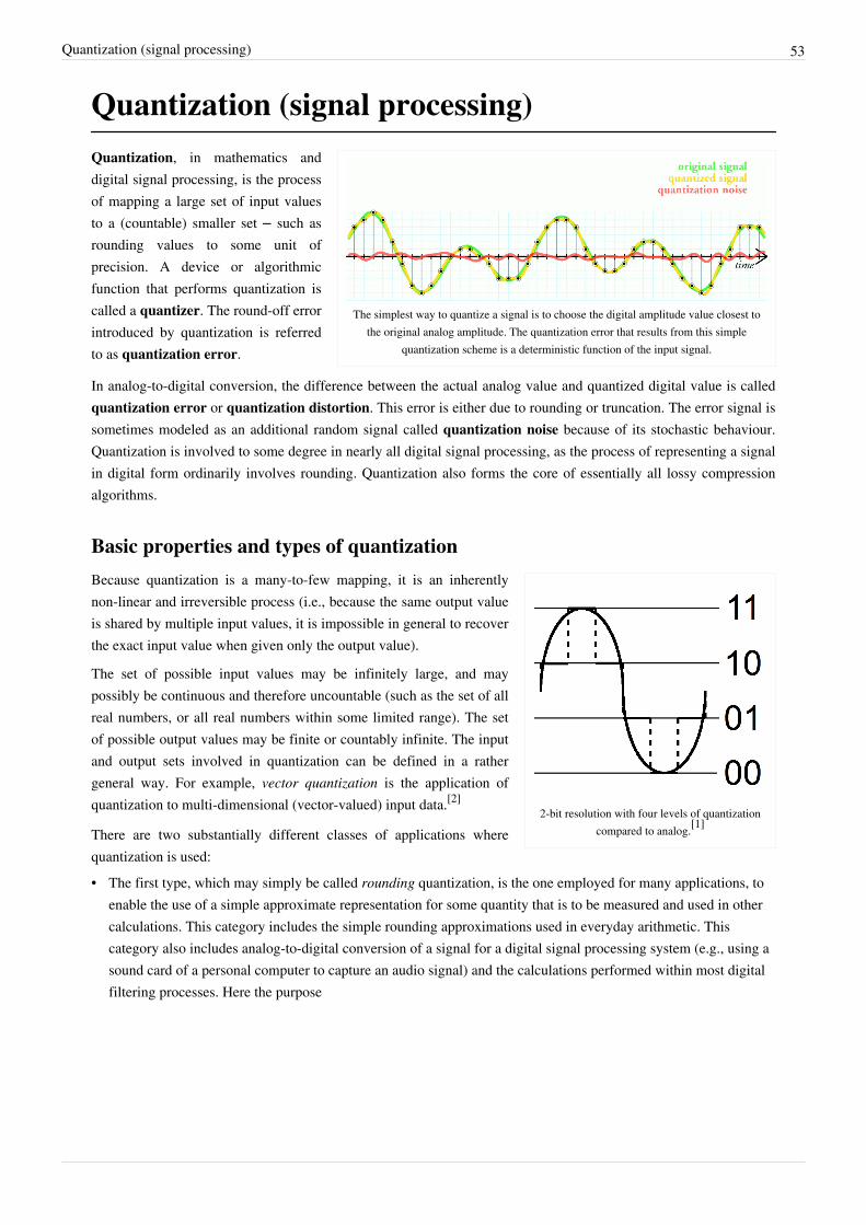
Quantization (signal processing) 53
Quantization (signal processing)
The simplest way to quantize a signal is to choose the digital amplitude value closest tothe original analog amplitude. The quantization error that results from this simple
quantization scheme is a deterministic function of the input signal.
Quantization, in mathematics anddigital signal processing, is the processof mapping a large set of input valuesto a (countable) smaller set – such asrounding values to some unit ofprecision. A device or algorithmicfunction that performs quantization iscalled a quantizer. The round-off errorintroduced by quantization is referredto as quantization error.
In analog-to-digital conversion, the difference between the actual analog value and quantized digital value is calledquantization error or quantization distortion. This error is either due to rounding or truncation. The error signal issometimes modeled as an additional random signal called quantization noise because of its stochastic behaviour.Quantization is involved to some degree in nearly all digital signal processing, as the process of representing a signalin digital form ordinarily involves rounding. Quantization also forms the core of essentially all lossy compressionalgorithms.
Basic properties and types of quantization
2-bit resolution with four levels of quantizationcompared to analog.[1]
Because quantization is a many-to-few mapping, it is an inherentlynon-linear and irreversible process (i.e., because the same output valueis shared by multiple input values, it is impossible in general to recoverthe exact input value when given only the output value).
The set of possible input values may be infinitely large, and maypossibly be continuous and therefore uncountable (such as the set of allreal numbers, or all real numbers within some limited range). The setof possible output values may be finite or countably infinite. The inputand output sets involved in quantization can be defined in a rathergeneral way. For example, vector quantization is the application ofquantization to multi-dimensional (vector-valued) input data.[2]
There are two substantially different classes of applications wherequantization is used:• The first type, which may simply be called rounding quantization, is the one employed for many applications, to
enable the use of a simple approximate representation for some quantity that is to be measured and used in othercalculations. This category includes the simple rounding approximations used in everyday arithmetic. Thiscategory also includes analog-to-digital conversion of a signal for a digital signal processing system (e.g., using asound card of a personal computer to capture an audio signal) and the calculations performed within most digitalfiltering processes. Here the purpose

Quantization (signal processing) 54
3-bit resolution with eight levels.
is primarily to retain as much signal fidelity as possible whileeliminating unnecessary precision and keeping the dynamic range ofthe signal within practical limits (to avoid signal clipping orarithmetic overflow). In such uses, substantial loss of signal fidelityis often unacceptable, and the design often centers around managingthe approximation error to ensure that very little distortion isintroduced.
• The second type, which can be called rate–distortion optimized quantization, is encountered in source coding for"lossy" data compression algorithms, where the purpose is to manage distortion within the limits of the bit ratesupported by a communication channel or storage medium. In this second setting, the amount of introduceddistortion may be managed carefully by sophisticated techniques, and introducing some significant amount ofdistortion may be unavoidable. A quantizer designed for this purpose may be quite different and more elaborate indesign than an ordinary rounding operation. It is in this domain that substantial rate–distortion theory analysis islikely to be applied. However, the same concepts actually apply in both use cases.
The analysis of quantization involves studying the amount of data (typically measured in digits or bits or bit rate)that is used to represent the output of the quantizer, and studying the loss of precision that is introduced by thequantization process (which is referred to as the distortion). The general field of such study of rate and distortion isknown as rate–distortion theory.
Scalar quantizationThe most common type of quantization is known as scalar quantization. Scalar quantization, typically denoted as
, is the process of using a quantization function ( ) to map a scalar (one-dimensional) input value to a scalar output value . Scalar quantization can be as simple and intuitive as rounding high-precision numbers tothe nearest integer, or to the nearest multiple of some other unit of precision (such as rounding a large monetaryamount to the nearest thousand dollars). Scalar quantization of continuous-valued input data that is performed by anelectronic sensor is referred to as analog-to-digital conversion. Analog-to-digital conversion often also involvessampling the signal periodically in time (e.g., at 44.1 kHz for CD-quality audio signals).
Rounding exampleAs an example, rounding a real number to the nearest integer value forms a very basic type of quantizer – auniform one. A typical (mid-tread) uniform quantizer with a quantization step size equal to some value can beexpressed as
,
where the function ( ) is the sign function (also known as the signum function). For simple rounding to the nearest integer, the step size is equal to 1. With or with equal to any other integer value, this quantizer has real-valued inputs and integer-valued outputs, although this property is not a necessity – a quantizer may also have an integer input domain and may also have non-integer output values. The essential property of a quantizer is that it has a countable set of possible output values that has fewer members than the set of possible input values. The members of the set of output values may have integer, rational, or real values (or even other possible
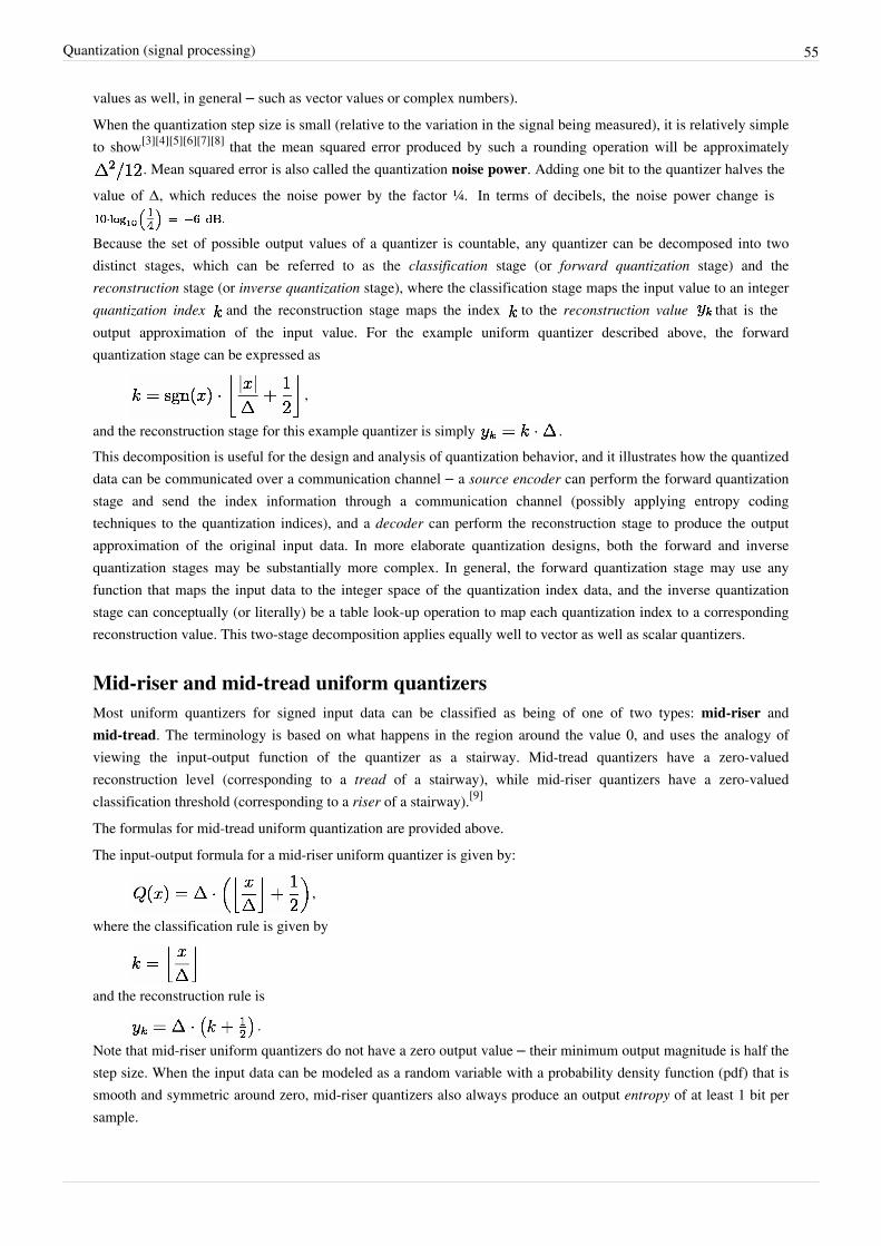
Quantization (signal processing) 55
values as well, in general – such as vector values or complex numbers).When the quantization step size is small (relative to the variation in the signal being measured), it is relatively simpleto show[3][4][5][6][7][8] that the mean squared error produced by such a rounding operation will be approximately
. Mean squared error is also called the quantization noise power. Adding one bit to the quantizer halves thevalue of Δ, which reduces the noise power by the factor ¼. In terms of decibels, the noise power change is
Because the set of possible output values of a quantizer is countable, any quantizer can be decomposed into twodistinct stages, which can be referred to as the classification stage (or forward quantization stage) and thereconstruction stage (or inverse quantization stage), where the classification stage maps the input value to an integerquantization index and the reconstruction stage maps the index to the reconstruction value that is theoutput approximation of the input value. For the example uniform quantizer described above, the forwardquantization stage can be expressed as
,
and the reconstruction stage for this example quantizer is simply .This decomposition is useful for the design and analysis of quantization behavior, and it illustrates how the quantizeddata can be communicated over a communication channel – a source encoder can perform the forward quantizationstage and send the index information through a communication channel (possibly applying entropy codingtechniques to the quantization indices), and a decoder can perform the reconstruction stage to produce the outputapproximation of the original input data. In more elaborate quantization designs, both the forward and inversequantization stages may be substantially more complex. In general, the forward quantization stage may use anyfunction that maps the input data to the integer space of the quantization index data, and the inverse quantizationstage can conceptually (or literally) be a table look-up operation to map each quantization index to a correspondingreconstruction value. This two-stage decomposition applies equally well to vector as well as scalar quantizers.
Mid-riser and mid-tread uniform quantizersMost uniform quantizers for signed input data can be classified as being of one of two types: mid-riser andmid-tread. The terminology is based on what happens in the region around the value 0, and uses the analogy ofviewing the input-output function of the quantizer as a stairway. Mid-tread quantizers have a zero-valuedreconstruction level (corresponding to a tread of a stairway), while mid-riser quantizers have a zero-valuedclassification threshold (corresponding to a riser of a stairway).[9]
The formulas for mid-tread uniform quantization are provided above.The input-output formula for a mid-riser uniform quantizer is given by:
,
where the classification rule is given by
and the reconstruction rule is
.Note that mid-riser uniform quantizers do not have a zero output value – their minimum output magnitude is half thestep size. When the input data can be modeled as a random variable with a probability density function (pdf) that issmooth and symmetric around zero, mid-riser quantizers also always produce an output entropy of at least 1 bit persample.

Quantization (signal processing) 56
In contrast, mid-tread quantizers do have a zero output level, and can reach arbitrarily low bit rates per sample forinput distributions that are symmetric and taper off at higher magnitudes. For some applications, having a zerooutput signal representation or supporting low output entropy may be a necessity. In such cases, using a mid-treaduniform quantizer may be appropriate while using a mid-riser one would not be.In general, a mid-riser or mid-tread quantizer may not actually be a uniform quantizer – i.e., the size of thequantizer's classification intervals may not all be the same, or the spacing between its possible output values may notall be the same. The distinguishing characteristic of a mid-riser quantizer is that it has a classification threshold valuethat is exactly zero, and the distinguishing characteristic of a mid-tread quantizer is that is it has a reconstructionvalue that is exactly zero.Another name for a mid-tread quantizer is dead-zone quantizer, and the classification region around the zero outputvalue of such a quantizer is referred to as the dead zone. The dead zone can sometimes serve the same purpose as anoise gate or squelch function.
Granular distortion and overload distortionOften the design of a quantizer involves supporting only a limited range of possible output values and performingclipping to limit the output to this range whenever the input exceeds the supported range. The error introduced bythis clipping is referred to as overload distortion. Within the extreme limits of the supported range, the amount ofspacing between the selectable output values of a quantizer is referred to as its granularity, and the error introducedby this spacing is referred to as granular distortion. It is common for the design of a quantizer to involve determiningthe proper balance between granular distortion and overload distortion. For a given supported number of possibleoutput values, reducing the average granular distortion may involve increasing the average overload distortion, andvice-versa. A technique for controlling the amplitude of the signal (or, equivalently, the quantization step size ) toachieve the appropriate balance is the use of automatic gain control (AGC). However, in some quantizer designs, theconcepts of granular error and overload error may not apply (e.g., for a quantizer with a limited range of input data orwith a countably infinite set of selectable output values).
The additive noise model for quantization errorA common assumption for the analysis of quantization error is that it affects a signal processing system in a similarmanner to that of additive white noise – having negligible correlation with the signal and an approximately flatpower spectral density.[10][11] The additive noise model is commonly used for the analysis of quantization erroreffects in digital filtering systems, and it can be very useful in such analysis. It has been shown to be a valid model incases of high resolution quantization (small relative to the signal strength) with smooth probability densityfunctions.[12] However, additive noise behaviour is not always a valid assumption, and care should be taken to avoidassuming that this model always applies. In actuality, the quantization error (for quantizers defined as describedhere) is deterministically related to the signal rather than being independent of it. Thus, periodic signals can createperiodic quantization noise. And in some cases it can even cause limit cycles to appear in digital signal processingsystems.One way to ensure effective independence of the quantization error from the source signal is to perform ditheredquantization (sometimes with noise shaping), which involves adding random (or pseudo-random) noise to the signalprior to quantization. This can sometimes be beneficial for such purposes as improving the subjective quality of theresult, however it can increase the total quantity of error introduced by the quantization process.
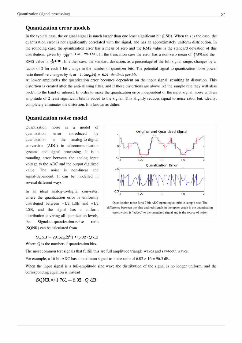
Quantization (signal processing) 57
Quantization error modelsIn the typical case, the original signal is much larger than one least significant bit (LSB). When this is the case, thequantization error is not significantly correlated with the signal, and has an approximately uniform distribution. Inthe rounding case, the quantization error has a mean of zero and the RMS value is the standard deviation of thisdistribution, given by . In the truncation case the error has a non-zero mean of and theRMS value is . In either case, the standard deviation, as a percentage of the full signal range, changes by afactor of 2 for each 1-bit change in the number of quantizer bits. The potential signal-to-quantization-noise powerratio therefore changes by 4, or decibels per bit.At lower amplitudes the quantization error becomes dependent on the input signal, resulting in distortion. Thisdistortion is created after the anti-aliasing filter, and if these distortions are above 1/2 the sample rate they will aliasback into the band of interest. In order to make the quantization error independent of the input signal, noise with anamplitude of 2 least significant bits is added to the signal. This slightly reduces signal to noise ratio, but, ideally,completely eliminates the distortion. It is known as dither.
Quantization noise model
Quantization noise for a 2-bit ADC operating at infinite sample rate. Thedifference between the blue and red signals in the upper graph is the quantization
error, which is "added" to the quantized signal and is the source of noise.
Quantization noise is a model ofquantization error introduced byquantization in the analog-to-digitalconversion (ADC) in telecommunicationsystems and signal processing. It is arounding error between the analog inputvoltage to the ADC and the output digitizedvalue. The noise is non-linear andsignal-dependent. It can be modelled inseveral different ways.
In an ideal analog-to-digital converter,where the quantization error is uniformlydistributed between −1/2 LSB and +1/2LSB, and the signal has a uniformdistribution covering all quantization levels,the Signal-to-quantization-noise ratio(SQNR) can be calculated from
Where Q is the number of quantization bits.The most common test signals that fulfill this are full amplitude triangle waves and sawtooth waves.For example, a 16-bit ADC has a maximum signal-to-noise ratio of 6.02 × 16 = 96.3 dB.When the input signal is a full-amplitude sine wave the distribution of the signal is no longer uniform, and thecorresponding equation is instead

Quantization (signal processing) 58
Comparison of quantizing a sinusoid to 64 levels (6 bits) and 256 levels (8 bits).The additive noise created by 6-bit quantization is 12 dB greater than the noisecreated by 8-bit quantization. When the spectral distribution is flat, as in this
example, the 12 dB difference manifests as a measurable difference in the noisefloors.
Here, the quantization noise is once againassumed to be uniformly distributed. Whenthe input signal has a high amplitude and awide frequency spectrum this is the case. Inthis case a 16-bit ADC has a maximumsignal-to-noise ratio of 98.09 dB. The 1.761difference in signal-to-noise only occurs dueto the signal being a full-scale sine waveinstead of a triangle/sawtooth.
Quantization noise power can be derivedfrom
where is the voltage of the level.(Typical real-life values are worse than this theoretical minimum, due to the addition of dither to reduce theobjectionable effects of quantization, and to imperfections of the ADC circuitry. On the other hand, specificationsoften use A-weighted measurements to hide the inaudible effects of noise shaping, which improves themeasurement.)For complex signals in high-resolution ADCs this is an accurate model. For low-resolution ADCs, low-level signalsin high-resolution ADCs, and for simple waveforms the quantization noise is not uniformly distributed, making thismodel inaccurate. In these cases the quantization noise distribution is strongly affected by the exact amplitude of thesignal.The calculations above, however, assume a completely filled input channel. If this is not the case - if the input signalis small - the relative quantization distortion can be very large. To circumvent this issue, analog compressors andexpanders can be used, but these introduce large amounts of distortion as well, especially if the compressor does notmatch the expander. The application of such compressors and expanders is also known as companding.
Rate–distortion quantizer designA scalar quantizer, which performs a quantization operation, can ordinarily be decomposed into two stages:
• Classification: A process that classifies the input signal range into non-overlapping intervals , bydefining boundary (decision) values , such that for , with the extreme limits defined by and . All the inputs that fall in a given intervalrange are associated with the same quantization index .• Reconstruction: Each interval is represented by a reconstruction value which implements the mapping
.These two stages together comprise the mathematical operation of .Entropy coding techniques can be applied to communicate the quantization indices from a source encoder thatperforms the classification stage to a decoder that performs the reconstruction stage. One way to do this is toassociate each quantization index with a binary codeword . An important consideration is the number of bitsused for each codeword, denoted here by .As a result, the design of an -level quantizer and an associated set of codewords for communicating its indexvalues requires finding the values of , and which optimally satisfy a selected set ofdesign constraints such as the bit rate and distortion .
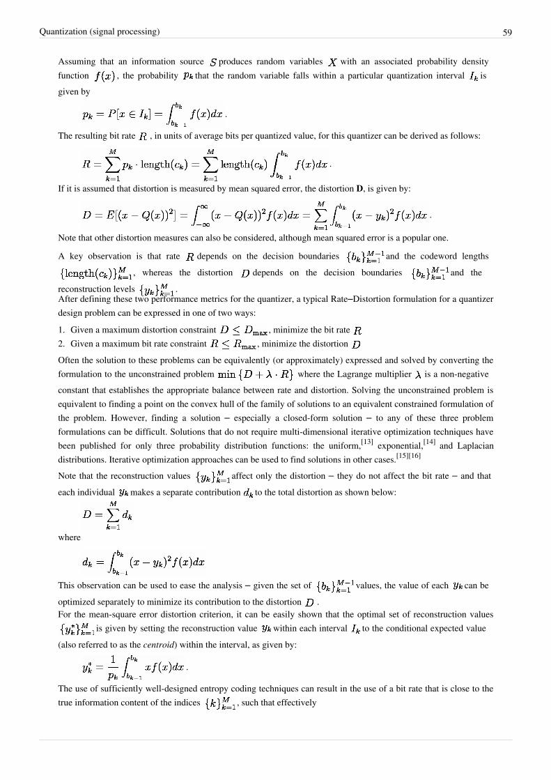
Quantization (signal processing) 59
Assuming that an information source produces random variables with an associated probability densityfunction , the probability that the random variable falls within a particular quantization interval isgiven by
.
The resulting bit rate , in units of average bits per quantized value, for this quantizer can be derived as follows:
.
If it is assumed that distortion is measured by mean squared error, the distortion D, is given by:
.
Note that other distortion measures can also be considered, although mean squared error is a popular one.
A key observation is that rate depends on the decision boundaries and the codeword lengths, whereas the distortion depends on the decision boundaries and the
reconstruction levels .After defining these two performance metrics for the quantizer, a typical Rate–Distortion formulation for a quantizerdesign problem can be expressed in one of two ways:1. Given a maximum distortion constraint , minimize the bit rate 2. Given a maximum bit rate constraint , minimize the distortion Often the solution to these problems can be equivalently (or approximately) expressed and solved by converting theformulation to the unconstrained problem where the Lagrange multiplier is a non-negativeconstant that establishes the appropriate balance between rate and distortion. Solving the unconstrained problem isequivalent to finding a point on the convex hull of the family of solutions to an equivalent constrained formulation ofthe problem. However, finding a solution – especially a closed-form solution – to any of these three problemformulations can be difficult. Solutions that do not require multi-dimensional iterative optimization techniques havebeen published for only three probability distribution functions: the uniform,[13] exponential,[14] and Laplaciandistributions. Iterative optimization approaches can be used to find solutions in other cases.[15][16]
Note that the reconstruction values affect only the distortion – they do not affect the bit rate – and thateach individual makes a separate contribution to the total distortion as shown below:
where
This observation can be used to ease the analysis – given the set of values, the value of each can beoptimized separately to minimize its contribution to the distortion .For the mean-square error distortion criterion, it can be easily shown that the optimal set of reconstruction values
is given by setting the reconstruction value within each interval to the conditional expected value(also referred to as the centroid) within the interval, as given by:
.
The use of sufficiently well-designed entropy coding techniques can result in the use of a bit rate that is close to thetrue information content of the indices , such that effectively
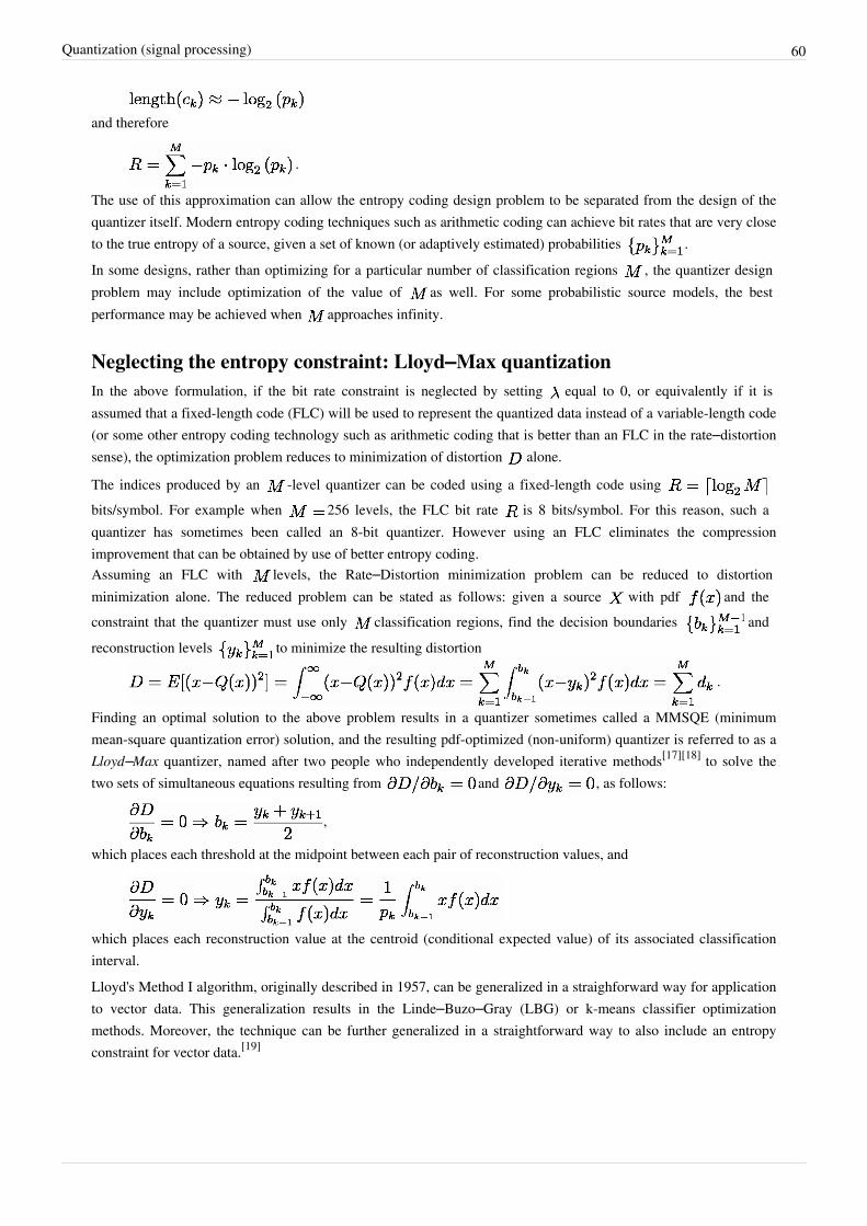
Quantization (signal processing) 60
and therefore
.
The use of this approximation can allow the entropy coding design problem to be separated from the design of thequantizer itself. Modern entropy coding techniques such as arithmetic coding can achieve bit rates that are very closeto the true entropy of a source, given a set of known (or adaptively estimated) probabilities .In some designs, rather than optimizing for a particular number of classification regions , the quantizer designproblem may include optimization of the value of as well. For some probabilistic source models, the bestperformance may be achieved when approaches infinity.
Neglecting the entropy constraint: Lloyd–Max quantizationIn the above formulation, if the bit rate constraint is neglected by setting equal to 0, or equivalently if it isassumed that a fixed-length code (FLC) will be used to represent the quantized data instead of a variable-length code(or some other entropy coding technology such as arithmetic coding that is better than an FLC in the rate–distortionsense), the optimization problem reduces to minimization of distortion alone.
The indices produced by an -level quantizer can be coded using a fixed-length code using bits/symbol. For example when 256 levels, the FLC bit rate is 8 bits/symbol. For this reason, such aquantizer has sometimes been called an 8-bit quantizer. However using an FLC eliminates the compressionimprovement that can be obtained by use of better entropy coding.Assuming an FLC with levels, the Rate–Distortion minimization problem can be reduced to distortionminimization alone. The reduced problem can be stated as follows: given a source with pdf and theconstraint that the quantizer must use only classification regions, find the decision boundaries andreconstruction levels to minimize the resulting distortion
.
Finding an optimal solution to the above problem results in a quantizer sometimes called a MMSQE (minimummean-square quantization error) solution, and the resulting pdf-optimized (non-uniform) quantizer is referred to as aLloyd–Max quantizer, named after two people who independently developed iterative methods[17][18] to solve thetwo sets of simultaneous equations resulting from and , as follows:
,
which places each threshold at the midpoint between each pair of reconstruction values, and
which places each reconstruction value at the centroid (conditional expected value) of its associated classificationinterval.Lloyd's Method I algorithm, originally described in 1957, can be generalized in a straighforward way for applicationto vector data. This generalization results in the Linde–Buzo–Gray (LBG) or k-means classifier optimizationmethods. Moreover, the technique can be further generalized in a straightforward way to also include an entropyconstraint for vector data.[19]

Quantization (signal processing) 61
Uniform quantization and the 6 dB/bit approximationThe Lloyd–Max quantizer is actually a uniform quantizer when the input pdf is uniformly distributed over the range
. However, for a source that does not have a uniform distribution, theminimum-distortion quantizer may not be a uniform quantizer.The analysis of a uniform quantizer applied to a uniformly distributed source can be summarized in what follows:
A symmetric source X can be modelled with , for and 0 elsewhere. The
step size and the signal to quantization noise ratio (SQNR) of the quantizer is
.
For a fixed-length code using bits, , resulting in,
or approximately 6 dB per bit. For example, for =8 bits, =256 levels and SQNR = 8*6 = 48 dB; and for =16 bits, =65536 and SQNR = 16*6 = 96 dB. The property of 6 dB improvement in SQNR for each extra bitused in quantization is a well-known figure of merit. However, it must be used with care: this derivation is only for auniform quantizer applied to a uniform source.For other source pdfs and other quantizer designs, the SQNR may be somewhat different from that predicted by 6dB/bit, depending on the type of pdf, the type of source, the type of quantizer, and the bit rate range of operation.However, it is common to assume that for many sources, the slope of a quantizer SQNR function can beapproximated as 6 dB/bit when operating at a sufficiently high bit rate. At asymptotically high bit rates, cutting thestep size in half increases the bit rate by approximately 1 bit per sample (because 1 bit is needed to indicate whetherthe value is in the left or right half of the prior double-sized interval) and reduces the mean squared error by a factorof 4 (i.e., 6 dB) based on the approximation.At asymptotically high bit rates, the 6 dB/bit approximation is supported for many source pdfs by rigoroustheoretical analysis. Moreover, the structure of the optimal scalar quantizer (in the rate–distortion sense) approachesthat of a uniform quantizer under these conditions.
Other fieldsMany physical quantities are actually quantized by physical entities. Examples of fields where this limitation appliesinclude electronics (due to electrons), optics (due to photons), biology (due to DNA), and chemistry (due tomolecules). This is sometimes known as the "quantum noise limit" of systems in those fields. This is a differentmanifestation of "quantization error," in which theoretical models may be analog but physically occurs digitally.Around the quantum limit, the distinction between analog and digital quantities vanishes.Wikipedia:Citation needed

Quantization (signal processing) 62
Notes[1] Hodgson, Jay (2010). Understanding Records, p.56. ISBN 978-1-4411-5607-5. Adapted from Franz, David (2004). Recording and Producing
in the Home Studio, p.38-9. Berklee Press.[2] Allen Gersho and Robert M. Gray, Vector Quantization and Signal Compression (http:/ / books. google. com/ books/ about/
Vector_Quantization_and_Signal_Compressi. html?id=DwcDm6xgItUC), Springer, ISBN 978-0-7923-9181-4, 1991.[3] William Fleetwood Sheppard, "On the Calculation of the Most Probable Values of Frequency Constants for data arranged according to
Equidistant Divisions of a Scale", Proceedings of the London Mathematical Society, Vol. 29, pp. 353–80, 1898.[4] W. R. Bennett, " Spectra of Quantized Signals (http:/ / www. alcatel-lucent. com/ bstj/ vol27-1948/ articles/ bstj27-3-446. pdf)", Bell System
Technical Journal, Vol. 27, pp. 446–472, July 1948.[5] B. M. Oliver, J. R. Pierce, and Claude E. Shannon, "The Philosophy of PCM", Proceedings of the IRE, Vol. 36, pp. 1324–1331, Nov. 1948.[6] Seymour Stein and J. Jay Jones, Modern Communication Principles (http:/ / books. google. com/ books/ about/
Modern_communication_principles. html?id=jBc3AQAAIAAJ), McGraw–Hill, ISBN 978-0-07-061003-3, 1967 (p. 196).[7] Herbert Gish and John N. Pierce, "Asymptotically Efficient Quantizing", IEEE Transactions on Information Theory, Vol. IT-14, No. 5, pp.
676–683, Sept. 1968.[8] Robert M. Gray and David L. Neuhoff, "Quantization", IEEE Transactions on Information Theory, Vol. IT-44, No. 6, pp. 2325–2383, Oct.
1998.[9] Allen Gersho, "Quantization", IEEE Communications Society Magazine, pp. 16–28, Sept. 1977.[10] Bernard Widrow, "A study of rough amplitude quantization by means of Nyquist sampling theory", IRE Trans. Circuit Theory, Vol. CT-3,
pp. 266–276, 1956.[11] Bernard Widrow, " Statistical analysis of amplitude quantized sampled data systems (http:/ / www-isl. stanford. edu/ ~widrow/ papers/
j1961statisticalanalysis. pdf)", Trans. AIEE Pt. II: Appl. Ind., Vol. 79, pp. 555–568, Jan. 1961.[12] Daniel Marco and David L. Neuhoff, "The Validity of the Additive Noise Model for Uniform Scalar Quantizers", IEEE Transactions on
Information Theory, Vol. IT-51, No. 5, pp. 1739–1755, May 2005.[13] Nariman Farvardin and James W. Modestino, "Optimum Quantizer Performance for a Class of Non-Gaussian Memoryless Sources", IEEE
Transactions on Information Theory, Vol. IT-30, No. 3, pp. 485–497, May 1982 (Section VI.C and Appendix B).[14] Gary J. Sullivan, "Efficient Scalar Quantization of Exponential and Laplacian Random Variables", IEEE Transactions on Information
Theory, Vol. IT-42, No. 5, pp. 1365–1374, Sept. 1996.[15] Toby Berger, "Optimum Quantizers and Permutation Codes", IEEE Transactions on Information Theory, Vol. IT-18, No. 6, pp. 759–765,
Nov. 1972.[16] Toby Berger, "Minimum Entropy Quantizers and Permutation Codes", IEEE Transactions on Information Theory, Vol. IT-28, No. 2, pp.
149–157, Mar. 1982.[17] Stuart P. Lloyd, "Least Squares Quantization in PCM", IEEE Transactions on Information Theory, Vol. IT-28, pp. 129–137, No. 2, March
1982 (work documented in a manuscript circulated for comments at Bell Laboratories with a department log date of 31 July 1957 and alsopresented at the 1957 meeting of the Institute of Mathematical Statistics, although not formally published until 1982).
[18] Joel Max, "Quantizing for Minimum Distortion", IRE Transactions on Information Theory, Vol. IT-6, pp. 7–12, March 1960.[19] Philip A. Chou, Tom Lookabaugh, and Robert M. Gray, "Entropy-Constrained Vector Quantization", IEEE Transactions on Acoustics,
Speech, and Signal Processing, Vol. ASSP-37, No. 1, Jan. 1989.
References• Sayood, Khalid (2005), Introduction to Data Compression, Third Edition, Morgan Kaufmann,
ISBN 978-0-12-620862-7• Jayant, Nikil S.; Noll, Peter (1984), Digital Coding of Waveforms: Principles and Applications to Speech and
Video, Prentice–Hall, ISBN 978-0-13-211913-9• Gregg, W. David (1977), Analog & Digital Communication, John Wiley, ISBN 978-0-471-32661-8• Stein, Seymour; Jones, J. Jay (1967), Modern Communication Principles, McGraw–Hill,
ISBN 978-0-07-061003-3
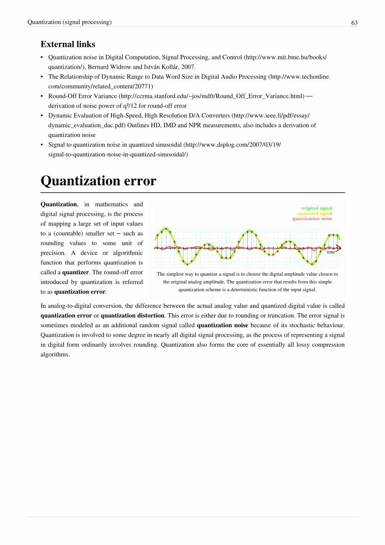
Quantization (signal processing) 63
External links• Quantization noise in Digital Computation, Signal Processing, and Control (http:/ / www. mit. bme. hu/ books/
quantization/ ), Bernard Widrow and István Kollár, 2007.• The Relationship of Dynamic Range to Data Word Size in Digital Audio Processing (http:/ / www. techonline.
com/ community/ related_content/ 20771)• Round-Off Error Variance (http:/ / ccrma. stanford. edu/ ~jos/ mdft/ Round_Off_Error_Variance. html) —
derivation of noise power of q²/12 for round-off error• Dynamic Evaluation of High-Speed, High Resolution D/A Converters (http:/ / www. ieee. li/ pdf/ essay/
dynamic_evaluation_dac. pdf) Outlines HD, IMD and NPR measurements, also includes a derivation ofquantization noise
• Signal to quantization noise in quantized sinusoidal (http:/ / www. dsplog. com/ 2007/ 03/ 19/signal-to-quantization-noise-in-quantized-sinusoidal/ )
Quantization error
The simplest way to quantize a signal is to choose the digital amplitude value closest tothe original analog amplitude. The quantization error that results from this simple
quantization scheme is a deterministic function of the input signal.
Quantization, in mathematics anddigital signal processing, is the processof mapping a large set of input valuesto a (countable) smaller set – such asrounding values to some unit ofprecision. A device or algorithmicfunction that performs quantization iscalled a quantizer. The round-off errorintroduced by quantization is referredto as quantization error.
In analog-to-digital conversion, the difference between the actual analog value and quantized digital value is calledquantization error or quantization distortion. This error is either due to rounding or truncation. The error signal issometimes modeled as an additional random signal called quantization noise because of its stochastic behaviour.Quantization is involved to some degree in nearly all digital signal processing, as the process of representing a signalin digital form ordinarily involves rounding. Quantization also forms the core of essentially all lossy compressionalgorithms.
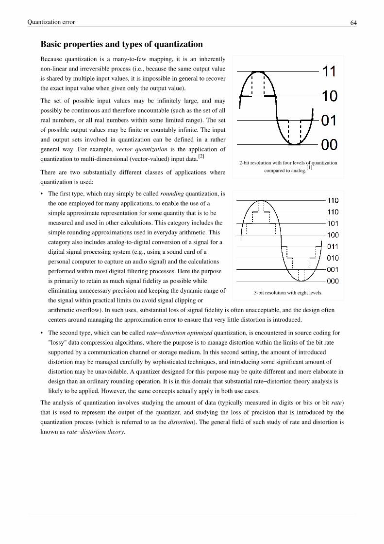
Quantization error 64
Basic properties and types of quantization
2-bit resolution with four levels of quantizationcompared to analog.[1]
3-bit resolution with eight levels.
Because quantization is a many-to-few mapping, it is an inherentlynon-linear and irreversible process (i.e., because the same output valueis shared by multiple input values, it is impossible in general to recoverthe exact input value when given only the output value).
The set of possible input values may be infinitely large, and maypossibly be continuous and therefore uncountable (such as the set of allreal numbers, or all real numbers within some limited range). The setof possible output values may be finite or countably infinite. The inputand output sets involved in quantization can be defined in a rathergeneral way. For example, vector quantization is the application ofquantization to multi-dimensional (vector-valued) input data.[2]
There are two substantially different classes of applications wherequantization is used:• The first type, which may simply be called rounding quantization, is
the one employed for many applications, to enable the use of asimple approximate representation for some quantity that is to bemeasured and used in other calculations. This category includes thesimple rounding approximations used in everyday arithmetic. Thiscategory also includes analog-to-digital conversion of a signal for adigital signal processing system (e.g., using a sound card of apersonal computer to capture an audio signal) and the calculationsperformed within most digital filtering processes. Here the purposeis primarily to retain as much signal fidelity as possible whileeliminating unnecessary precision and keeping the dynamic range ofthe signal within practical limits (to avoid signal clipping orarithmetic overflow). In such uses, substantial loss of signal fidelity is often unacceptable, and the design oftencenters around managing the approximation error to ensure that very little distortion is introduced.
• The second type, which can be called rate–distortion optimized quantization, is encountered in source coding for"lossy" data compression algorithms, where the purpose is to manage distortion within the limits of the bit ratesupported by a communication channel or storage medium. In this second setting, the amount of introduceddistortion may be managed carefully by sophisticated techniques, and introducing some significant amount ofdistortion may be unavoidable. A quantizer designed for this purpose may be quite different and more elaborate indesign than an ordinary rounding operation. It is in this domain that substantial rate–distortion theory analysis islikely to be applied. However, the same concepts actually apply in both use cases.
The analysis of quantization involves studying the amount of data (typically measured in digits or bits or bit rate)that is used to represent the output of the quantizer, and studying the loss of precision that is introduced by thequantization process (which is referred to as the distortion). The general field of such study of rate and distortion isknown as rate–distortion theory.
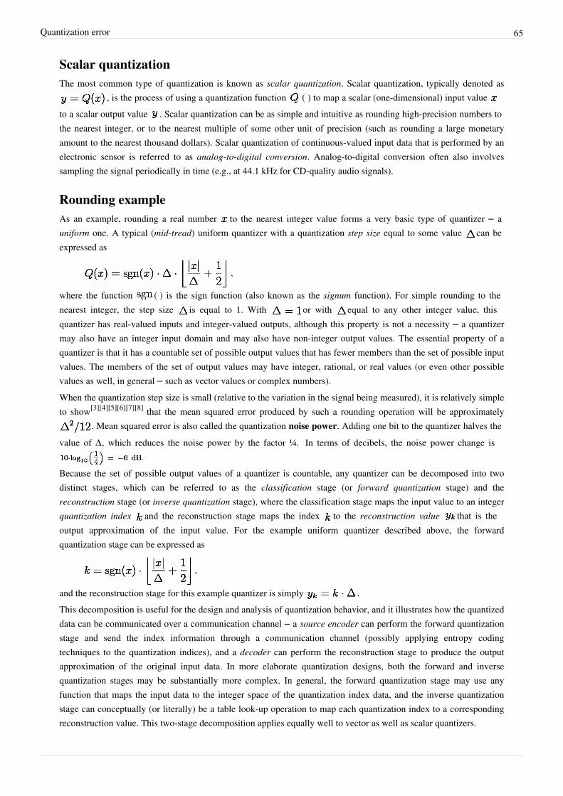
Quantization error 65
Scalar quantizationThe most common type of quantization is known as scalar quantization. Scalar quantization, typically denoted as
, is the process of using a quantization function ( ) to map a scalar (one-dimensional) input value to a scalar output value . Scalar quantization can be as simple and intuitive as rounding high-precision numbers tothe nearest integer, or to the nearest multiple of some other unit of precision (such as rounding a large monetaryamount to the nearest thousand dollars). Scalar quantization of continuous-valued input data that is performed by anelectronic sensor is referred to as analog-to-digital conversion. Analog-to-digital conversion often also involvessampling the signal periodically in time (e.g., at 44.1 kHz for CD-quality audio signals).
Rounding exampleAs an example, rounding a real number to the nearest integer value forms a very basic type of quantizer – auniform one. A typical (mid-tread) uniform quantizer with a quantization step size equal to some value can beexpressed as
,
where the function ( ) is the sign function (also known as the signum function). For simple rounding to thenearest integer, the step size is equal to 1. With or with equal to any other integer value, thisquantizer has real-valued inputs and integer-valued outputs, although this property is not a necessity – a quantizermay also have an integer input domain and may also have non-integer output values. The essential property of aquantizer is that it has a countable set of possible output values that has fewer members than the set of possible inputvalues. The members of the set of output values may have integer, rational, or real values (or even other possiblevalues as well, in general – such as vector values or complex numbers).When the quantization step size is small (relative to the variation in the signal being measured), it is relatively simpleto show[3][4][5][6][7][8] that the mean squared error produced by such a rounding operation will be approximately
. Mean squared error is also called the quantization noise power. Adding one bit to the quantizer halves thevalue of Δ, which reduces the noise power by the factor ¼. In terms of decibels, the noise power change is
Because the set of possible output values of a quantizer is countable, any quantizer can be decomposed into twodistinct stages, which can be referred to as the classification stage (or forward quantization stage) and thereconstruction stage (or inverse quantization stage), where the classification stage maps the input value to an integerquantization index and the reconstruction stage maps the index to the reconstruction value that is theoutput approximation of the input value. For the example uniform quantizer described above, the forwardquantization stage can be expressed as
,
and the reconstruction stage for this example quantizer is simply .This decomposition is useful for the design and analysis of quantization behavior, and it illustrates how the quantizeddata can be communicated over a communication channel – a source encoder can perform the forward quantizationstage and send the index information through a communication channel (possibly applying entropy codingtechniques to the quantization indices), and a decoder can perform the reconstruction stage to produce the outputapproximation of the original input data. In more elaborate quantization designs, both the forward and inversequantization stages may be substantially more complex. In general, the forward quantization stage may use anyfunction that maps the input data to the integer space of the quantization index data, and the inverse quantizationstage can conceptually (or literally) be a table look-up operation to map each quantization index to a correspondingreconstruction value. This two-stage decomposition applies equally well to vector as well as scalar quantizers.
Quantization error 66
Mid-riser and mid-tread uniform quantizersMost uniform quantizers for signed input data can be classified as being of one of two types: mid-riser andmid-tread. The terminology is based on what happens in the region around the value 0, and uses the analogy ofviewing the input-output function of the quantizer as a stairway. Mid-tread quantizers have a zero-valuedreconstruction level (corresponding to a tread of a stairway), while mid-riser quantizers have a zero-valuedclassification threshold (corresponding to a riser of a stairway).[9]
The formulas for mid-tread uniform quantization are provided above.The input-output formula for a mid-riser uniform quantizer is given by:
,
where the classification rule is given by
and the reconstruction rule is
.Note that mid-riser uniform quantizers do not have a zero output value – their minimum output magnitude is half thestep size. When the input data can be modeled as a random variable with a probability density function (pdf) that issmooth and symmetric around zero, mid-riser quantizers also always produce an output entropy of at least 1 bit persample.In contrast, mid-tread quantizers do have a zero output level, and can reach arbitrarily low bit rates per sample forinput distributions that are symmetric and taper off at higher magnitudes. For some applications, having a zerooutput signal representation or supporting low output entropy may be a necessity. In such cases, using a mid-treaduniform quantizer may be appropriate while using a mid-riser one would not be.In general, a mid-riser or mid-tread quantizer may not actually be a uniform quantizer – i.e., the size of thequantizer's classification intervals may not all be the same, or the spacing between its possible output values may notall be the same. The distinguishing characteristic of a mid-riser quantizer is that it has a classification threshold valuethat is exactly zero, and the distinguishing characteristic of a mid-tread quantizer is that is it has a reconstructionvalue that is exactly zero.Another name for a mid-tread quantizer is dead-zone quantizer, and the classification region around the zero outputvalue of such a quantizer is referred to as the dead zone. The dead zone can sometimes serve the same purpose as anoise gate or squelch function.
Granular distortion and overload distortionOften the design of a quantizer involves supporting only a limited range of possible output values and performingclipping to limit the output to this range whenever the input exceeds the supported range. The error introduced bythis clipping is referred to as overload distortion. Within the extreme limits of the supported range, the amount ofspacing between the selectable output values of a quantizer is referred to as its granularity, and the error introducedby this spacing is referred to as granular distortion. It is common for the design of a quantizer to involve determiningthe proper balance between granular distortion and overload distortion. For a given supported number of possibleoutput values, reducing the average granular distortion may involve increasing the average overload distortion, andvice-versa. A technique for controlling the amplitude of the signal (or, equivalently, the quantization step size ) toachieve the appropriate balance is the use of automatic gain control (AGC). However, in some quantizer designs, theconcepts of granular error and overload error may not apply (e.g., for a quantizer with a limited range of input data orwith a countably infinite set of selectable output values).
Quantization error 67
The additive noise model for quantization errorA common assumption for the analysis of quantization error is that it affects a signal processing system in a similarmanner to that of additive white noise – having negligible correlation with the signal and an approximately flatpower spectral density.[10][11] The additive noise model is commonly used for the analysis of quantization erroreffects in digital filtering systems, and it can be very useful in such analysis. It has been shown to be a valid model incases of high resolution quantization (small relative to the signal strength) with smooth probability densityfunctions.[12] However, additive noise behaviour is not always a valid assumption, and care should be taken to avoidassuming that this model always applies. In actuality, the quantization error (for quantizers defined as describedhere) is deterministically related to the signal rather than being independent of it. Thus, periodic signals can createperiodic quantization noise. And in some cases it can even cause limit cycles to appear in digital signal processingsystems.One way to ensure effective independence of the quantization error from the source signal is to perform ditheredquantization (sometimes with noise shaping), which involves adding random (or pseudo-random) noise to the signalprior to quantization. This can sometimes be beneficial for such purposes as improving the subjective quality of theresult, however it can increase the total quantity of error introduced by the quantization process.
Quantization error modelsIn the typical case, the original signal is much larger than one least significant bit (LSB). When this is the case, thequantization error is not significantly correlated with the signal, and has an approximately uniform distribution. Inthe rounding case, the quantization error has a mean of zero and the RMS value is the standard deviation of thisdistribution, given by . In the truncation case the error has a non-zero mean of and theRMS value is . In either case, the standard deviation, as a percentage of the full signal range, changes by afactor of 2 for each 1-bit change in the number of quantizer bits. The potential signal-to-quantization-noise powerratio therefore changes by 4, or decibels per bit.At lower amplitudes the quantization error becomes dependent on the input signal, resulting in distortion. Thisdistortion is created after the anti-aliasing filter, and if these distortions are above 1/2 the sample rate they will aliasback into the band of interest. In order to make the quantization error independent of the input signal, noise with anamplitude of 2 least significant bits is added to the signal. This slightly reduces signal to noise ratio, but, ideally,completely eliminates the distortion. It is known as dither.
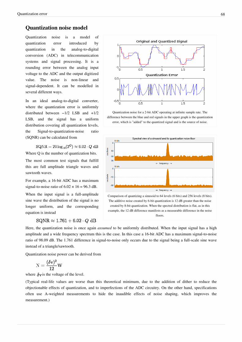
Quantization error 68
Quantization noise model
Quantization noise for a 2-bit ADC operating at infinite sample rate. Thedifference between the blue and red signals in the upper graph is the quantization
error, which is "added" to the quantized signal and is the source of noise.
Comparison of quantizing a sinusoid to 64 levels (6 bits) and 256 levels (8 bits).The additive noise created by 6-bit quantization is 12 dB greater than the noisecreated by 8-bit quantization. When the spectral distribution is flat, as in this
example, the 12 dB difference manifests as a measurable difference in the noisefloors.
Quantization noise is a model ofquantization error introduced byquantization in the analog-to-digitalconversion (ADC) in telecommunicationsystems and signal processing. It is arounding error between the analog inputvoltage to the ADC and the output digitizedvalue. The noise is non-linear andsignal-dependent. It can be modelled inseveral different ways.
In an ideal analog-to-digital converter,where the quantization error is uniformlydistributed between −1/2 LSB and +1/2LSB, and the signal has a uniformdistribution covering all quantization levels,the Signal-to-quantization-noise ratio(SQNR) can be calculated from
Where Q is the number of quantization bits.The most common test signals that fulfillthis are full amplitude triangle waves andsawtooth waves.
For example, a 16-bit ADC has a maximumsignal-to-noise ratio of 6.02 × 16 = 96.3 dB.
When the input signal is a full-amplitudesine wave the distribution of the signal is nolonger uniform, and the correspondingequation is instead
Here, the quantization noise is once again assumed to be uniformly distributed. When the input signal has a highamplitude and a wide frequency spectrum this is the case. In this case a 16-bit ADC has a maximum signal-to-noiseratio of 98.09 dB. The 1.761 difference in signal-to-noise only occurs due to the signal being a full-scale sine waveinstead of a triangle/sawtooth.
Quantization noise power can be derived from
where is the voltage of the level.(Typical real-life values are worse than this theoretical minimum, due to the addition of dither to reduce theobjectionable effects of quantization, and to imperfections of the ADC circuitry. On the other hand, specificationsoften use A-weighted measurements to hide the inaudible effects of noise shaping, which improves themeasurement.)

Quantization error 69
For complex signals in high-resolution ADCs this is an accurate model. For low-resolution ADCs, low-level signalsin high-resolution ADCs, and for simple waveforms the quantization noise is not uniformly distributed, making thismodel inaccurate. In these cases the quantization noise distribution is strongly affected by the exact amplitude of thesignal.The calculations above, however, assume a completely filled input channel. If this is not the case - if the input signalis small - the relative quantization distortion can be very large. To circumvent this issue, analog compressors andexpanders can be used, but these introduce large amounts of distortion as well, especially if the compressor does notmatch the expander. The application of such compressors and expanders is also known as companding.
Rate–distortion quantizer designA scalar quantizer, which performs a quantization operation, can ordinarily be decomposed into two stages:
• Classification: A process that classifies the input signal range into non-overlapping intervals , bydefining boundary (decision) values , such that for , with the extreme limits defined by and . All the inputs that fall in a given intervalrange are associated with the same quantization index .• Reconstruction: Each interval is represented by a reconstruction value which implements the mapping
.These two stages together comprise the mathematical operation of .Entropy coding techniques can be applied to communicate the quantization indices from a source encoder thatperforms the classification stage to a decoder that performs the reconstruction stage. One way to do this is toassociate each quantization index with a binary codeword . An important consideration is the number of bitsused for each codeword, denoted here by .As a result, the design of an -level quantizer and an associated set of codewords for communicating its indexvalues requires finding the values of , and which optimally satisfy a selected set ofdesign constraints such as the bit rate and distortion .Assuming that an information source produces random variables with an associated probability densityfunction , the probability that the random variable falls within a particular quantization interval isgiven by
.
The resulting bit rate , in units of average bits per quantized value, for this quantizer can be derived as follows:
.
If it is assumed that distortion is measured by mean squared error, the distortion D, is given by:
.
Note that other distortion measures can also be considered, although mean squared error is a popular one.
A key observation is that rate depends on the decision boundaries and the codeword lengths, whereas the distortion depends on the decision boundaries and the
reconstruction levels .After defining these two performance metrics for the quantizer, a typical Rate–Distortion formulation for a quantizerdesign problem can be expressed in one of two ways:1. Given a maximum distortion constraint , minimize the bit rate
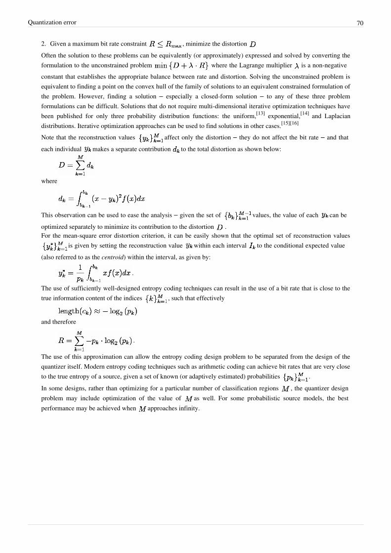
Quantization error 70
2. Given a maximum bit rate constraint , minimize the distortion Often the solution to these problems can be equivalently (or approximately) expressed and solved by converting theformulation to the unconstrained problem where the Lagrange multiplier is a non-negativeconstant that establishes the appropriate balance between rate and distortion. Solving the unconstrained problem isequivalent to finding a point on the convex hull of the family of solutions to an equivalent constrained formulation ofthe problem. However, finding a solution – especially a closed-form solution – to any of these three problemformulations can be difficult. Solutions that do not require multi-dimensional iterative optimization techniques havebeen published for only three probability distribution functions: the uniform,[13] exponential,[14] and Laplaciandistributions. Iterative optimization approaches can be used to find solutions in other cases.[15][16]
Note that the reconstruction values affect only the distortion – they do not affect the bit rate – and thateach individual makes a separate contribution to the total distortion as shown below:
where
This observation can be used to ease the analysis – given the set of values, the value of each can beoptimized separately to minimize its contribution to the distortion .For the mean-square error distortion criterion, it can be easily shown that the optimal set of reconstruction values
is given by setting the reconstruction value within each interval to the conditional expected value(also referred to as the centroid) within the interval, as given by:
.
The use of sufficiently well-designed entropy coding techniques can result in the use of a bit rate that is close to thetrue information content of the indices , such that effectively
and therefore
.
The use of this approximation can allow the entropy coding design problem to be separated from the design of thequantizer itself. Modern entropy coding techniques such as arithmetic coding can achieve bit rates that are very closeto the true entropy of a source, given a set of known (or adaptively estimated) probabilities .In some designs, rather than optimizing for a particular number of classification regions , the quantizer designproblem may include optimization of the value of as well. For some probabilistic source models, the bestperformance may be achieved when approaches infinity.
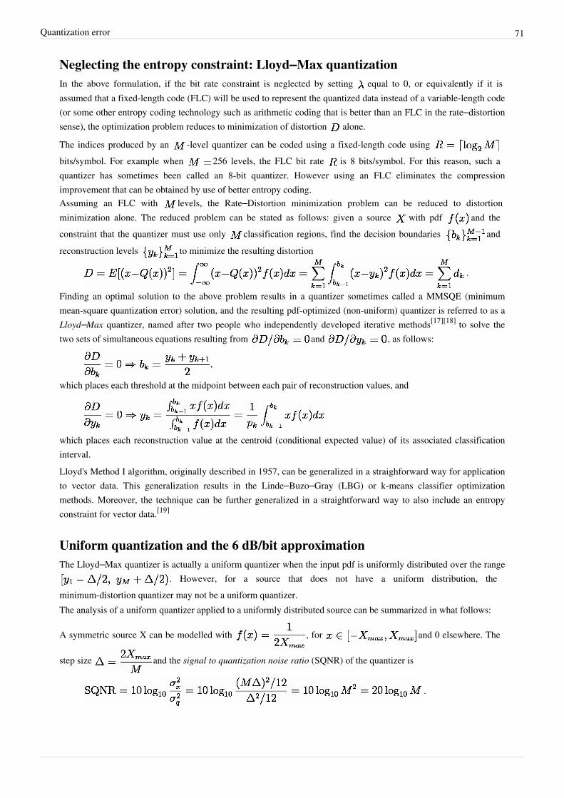
Quantization error 71
Neglecting the entropy constraint: Lloyd–Max quantizationIn the above formulation, if the bit rate constraint is neglected by setting equal to 0, or equivalently if it isassumed that a fixed-length code (FLC) will be used to represent the quantized data instead of a variable-length code(or some other entropy coding technology such as arithmetic coding that is better than an FLC in the rate–distortionsense), the optimization problem reduces to minimization of distortion alone.
The indices produced by an -level quantizer can be coded using a fixed-length code using bits/symbol. For example when 256 levels, the FLC bit rate is 8 bits/symbol. For this reason, such aquantizer has sometimes been called an 8-bit quantizer. However using an FLC eliminates the compressionimprovement that can be obtained by use of better entropy coding.Assuming an FLC with levels, the Rate–Distortion minimization problem can be reduced to distortionminimization alone. The reduced problem can be stated as follows: given a source with pdf and theconstraint that the quantizer must use only classification regions, find the decision boundaries andreconstruction levels to minimize the resulting distortion
.
Finding an optimal solution to the above problem results in a quantizer sometimes called a MMSQE (minimummean-square quantization error) solution, and the resulting pdf-optimized (non-uniform) quantizer is referred to as aLloyd–Max quantizer, named after two people who independently developed iterative methods[17][18] to solve thetwo sets of simultaneous equations resulting from and , as follows:
,
which places each threshold at the midpoint between each pair of reconstruction values, and
which places each reconstruction value at the centroid (conditional expected value) of its associated classificationinterval.Lloyd's Method I algorithm, originally described in 1957, can be generalized in a straighforward way for applicationto vector data. This generalization results in the Linde–Buzo–Gray (LBG) or k-means classifier optimizationmethods. Moreover, the technique can be further generalized in a straightforward way to also include an entropyconstraint for vector data.[19]
Uniform quantization and the 6 dB/bit approximationThe Lloyd–Max quantizer is actually a uniform quantizer when the input pdf is uniformly distributed over the range
. However, for a source that does not have a uniform distribution, theminimum-distortion quantizer may not be a uniform quantizer.The analysis of a uniform quantizer applied to a uniformly distributed source can be summarized in what follows:
A symmetric source X can be modelled with , for and 0 elsewhere. The
step size and the signal to quantization noise ratio (SQNR) of the quantizer is
.

Quantization error 72
For a fixed-length code using bits, , resulting in,
or approximately 6 dB per bit. For example, for =8 bits, =256 levels and SQNR = 8*6 = 48 dB; and for =16 bits, =65536 and SQNR = 16*6 = 96 dB. The property of 6 dB improvement in SQNR for each extra bitused in quantization is a well-known figure of merit. However, it must be used with care: this derivation is only for auniform quantizer applied to a uniform source.For other source pdfs and other quantizer designs, the SQNR may be somewhat different from that predicted by 6dB/bit, depending on the type of pdf, the type of source, the type of quantizer, and the bit rate range of operation.However, it is common to assume that for many sources, the slope of a quantizer SQNR function can beapproximated as 6 dB/bit when operating at a sufficiently high bit rate. At asymptotically high bit rates, cutting thestep size in half increases the bit rate by approximately 1 bit per sample (because 1 bit is needed to indicate whetherthe value is in the left or right half of the prior double-sized interval) and reduces the mean squared error by a factorof 4 (i.e., 6 dB) based on the approximation.At asymptotically high bit rates, the 6 dB/bit approximation is supported for many source pdfs by rigoroustheoretical analysis. Moreover, the structure of the optimal scalar quantizer (in the rate–distortion sense) approachesthat of a uniform quantizer under these conditions.
Other fieldsMany physical quantities are actually quantized by physical entities. Examples of fields where this limitation appliesinclude electronics (due to electrons), optics (due to photons), biology (due to DNA), and chemistry (due tomolecules). This is sometimes known as the "quantum noise limit" of systems in those fields. This is a differentmanifestation of "quantization error," in which theoretical models may be analog but physically occurs digitally.Around the quantum limit, the distinction between analog and digital quantities vanishes.Wikipedia:Citation needed
Notes[1] Hodgson, Jay (2010). Understanding Records, p.56. ISBN 978-1-4411-5607-5. Adapted from Franz, David (2004). Recording and Producing
in the Home Studio, p.38-9. Berklee Press.[2] Allen Gersho and Robert M. Gray, Vector Quantization and Signal Compression (http:/ / books. google. com/ books/ about/
Vector_Quantization_and_Signal_Compressi. html?id=DwcDm6xgItUC), Springer, ISBN 978-0-7923-9181-4, 1991.[3] William Fleetwood Sheppard, "On the Calculation of the Most Probable Values of Frequency Constants for data arranged according to
Equidistant Divisions of a Scale", Proceedings of the London Mathematical Society, Vol. 29, pp. 353–80, 1898.[4] W. R. Bennett, " Spectra of Quantized Signals (http:/ / www. alcatel-lucent. com/ bstj/ vol27-1948/ articles/ bstj27-3-446. pdf)", Bell System
Technical Journal, Vol. 27, pp. 446–472, July 1948.[5] B. M. Oliver, J. R. Pierce, and Claude E. Shannon, "The Philosophy of PCM", Proceedings of the IRE, Vol. 36, pp. 1324–1331, Nov. 1948.[6] Seymour Stein and J. Jay Jones, Modern Communication Principles (http:/ / books. google. com/ books/ about/
Modern_communication_principles. html?id=jBc3AQAAIAAJ), McGraw–Hill, ISBN 978-0-07-061003-3, 1967 (p. 196).[7] Herbert Gish and John N. Pierce, "Asymptotically Efficient Quantizing", IEEE Transactions on Information Theory, Vol. IT-14, No. 5, pp.
676–683, Sept. 1968.[8] Robert M. Gray and David L. Neuhoff, "Quantization", IEEE Transactions on Information Theory, Vol. IT-44, No. 6, pp. 2325–2383, Oct.
1998.[9] Allen Gersho, "Quantization", IEEE Communications Society Magazine, pp. 16–28, Sept. 1977.[10] Bernard Widrow, "A study of rough amplitude quantization by means of Nyquist sampling theory", IRE Trans. Circuit Theory, Vol. CT-3,
pp. 266–276, 1956.[11] Bernard Widrow, " Statistical analysis of amplitude quantized sampled data systems (http:/ / www-isl. stanford. edu/ ~widrow/ papers/
j1961statisticalanalysis. pdf)", Trans. AIEE Pt. II: Appl. Ind., Vol. 79, pp. 555–568, Jan. 1961.[12] Daniel Marco and David L. Neuhoff, "The Validity of the Additive Noise Model for Uniform Scalar Quantizers", IEEE Transactions on
Information Theory, Vol. IT-51, No. 5, pp. 1739–1755, May 2005.[13] Nariman Farvardin and James W. Modestino, "Optimum Quantizer Performance for a Class of Non-Gaussian Memoryless Sources", IEEE
Transactions on Information Theory, Vol. IT-30, No. 3, pp. 485–497, May 1982 (Section VI.C and Appendix B).[14] Gary J. Sullivan, "Efficient Scalar Quantization of Exponential and Laplacian Random Variables", IEEE Transactions on Information
Theory, Vol. IT-42, No. 5, pp. 1365–1374, Sept. 1996.
Quantization error 73
[15] Toby Berger, "Optimum Quantizers and Permutation Codes", IEEE Transactions on Information Theory, Vol. IT-18, No. 6, pp. 759–765,Nov. 1972.
[16] Toby Berger, "Minimum Entropy Quantizers and Permutation Codes", IEEE Transactions on Information Theory, Vol. IT-28, No. 2, pp.149–157, Mar. 1982.
[17] Stuart P. Lloyd, "Least Squares Quantization in PCM", IEEE Transactions on Information Theory, Vol. IT-28, pp. 129–137, No. 2, March1982 (work documented in a manuscript circulated for comments at Bell Laboratories with a department log date of 31 July 1957 and alsopresented at the 1957 meeting of the Institute of Mathematical Statistics, although not formally published until 1982).
[18] Joel Max, "Quantizing for Minimum Distortion", IRE Transactions on Information Theory, Vol. IT-6, pp. 7–12, March 1960.[19] Philip A. Chou, Tom Lookabaugh, and Robert M. Gray, "Entropy-Constrained Vector Quantization", IEEE Transactions on Acoustics,
Speech, and Signal Processing, Vol. ASSP-37, No. 1, Jan. 1989.
References• Sayood, Khalid (2005), Introduction to Data Compression, Third Edition, Morgan Kaufmann,
ISBN 978-0-12-620862-7• Jayant, Nikil S.; Noll, Peter (1984), Digital Coding of Waveforms: Principles and Applications to Speech and
Video, Prentice–Hall, ISBN 978-0-13-211913-9• Gregg, W. David (1977), Analog & Digital Communication, John Wiley, ISBN 978-0-471-32661-8• Stein, Seymour; Jones, J. Jay (1967), Modern Communication Principles, McGraw–Hill,
ISBN 978-0-07-061003-3
External links• Quantization noise in Digital Computation, Signal Processing, and Control (http:/ / www. mit. bme. hu/ books/
quantization/ ), Bernard Widrow and István Kollár, 2007.• The Relationship of Dynamic Range to Data Word Size in Digital Audio Processing (http:/ / www. techonline.
com/ community/ related_content/ 20771)• Round-Off Error Variance (http:/ / ccrma. stanford. edu/ ~jos/ mdft/ Round_Off_Error_Variance. html) —
derivation of noise power of q²/12 for round-off error• Dynamic Evaluation of High-Speed, High Resolution D/A Converters (http:/ / www. ieee. li/ pdf/ essay/
dynamic_evaluation_dac. pdf) Outlines HD, IMD and NPR measurements, also includes a derivation ofquantization noise
• Signal to quantization noise in quantized sinusoidal (http:/ / www. dsplog. com/ 2007/ 03/ 19/signal-to-quantization-noise-in-quantized-sinusoidal/ )

ENOB 74
ENOBEffective number of bits (ENOB) is a measure of the dynamic performance of an analog-to-digital converter(ADC) and its associated circuitry. The resolution of an ADC is specified by the number of bits used to represent theanalog value, in principle giving 2N signal levels for an N-bit signal. However, all real ADC circuits introduce noiseand distortion. ENOB specifies the resolution of an ideal ADC circuit that would have the same resolution as thecircuit under consideration.ENOB is also used as a quality measure for other blocks such as sample-and-hold amplifiers. This way, analogblocks can be easily included in signal-chain calculations as the total ENOB of a chain of blocks is usually below theENOB of the worst block.
DefinitionAn often used definition for ENOB is[1]
,
where all values are given in dB and:• SINAD is the ratio indicating the quality of the signal.• The 6.02 term in the divisor converts decibels (a log10 representation) to bits (a log2 representation).[2]
• The 1.76 term comes from quantization error in an ideal ADC.[3]</ref>This definition compares the SINAD of an ideal ADC or DAC with a word length of ENOB bits with the SINAD ofthe ADC or DAC being tested.
Notes[1][1] , Equation 1.[2][2] UNIQ-math-0-fdcc463dc40e329d-QINU
[3] <ref>Eq. 2.8 in "Design of multi-bit delta-sigma A/D converters", Yves Geerts, Michiel Steyaert,
Willy M. C. Sansen, 2002.
References• Gielen, Georges (2006). Analog Building Blocks for Signal Processing. Leuven: KULeuven-ESAT-MICAS.• Kester, Walt (2009), Understand SINAD, ENOB, SNR, THD, THD + N, and SFDR so You Don't Get Lost in the
Noise Floor (http:/ / www. analog. com/ static/ imported-files/ tutorials/ MT-003. pdf), Tutorial, Analog Devices,MT-003
• Maxim (December 17, 2001), Glossary of Frequently Used High-Speed Data Converter Terms (http:/ / www.maxim-ic. com/ appnotes. cfm/ appnote_number/ 740/ ), Application Note, Maxim, 740
External links• Video tutorial on ENOB (http:/ / e2e. ti. com/ videos/ m/ analog/ 97246. aspx) from Texas Instruments• The Effective Number of Bits (ENOB) (http:/ / www. rohde-schwarz. com/ appnote/ 1ER03. pdf) - This
application note explains how to measure the oscilloscope ENOB.

Sampling rate 75
Sampling rate
Signal sampling representation. The continuous signal is represented with a greencolored line while the discrete samples are indicated by the blue vertical lines.
In signal processing, sampling is thereduction of a continuous signal to a discretesignal. A common example is theconversion of a sound wave (a continuoussignal) to a sequence of samples (adiscrete-time signal).
A sample refers to a value or set of values ata point in time and/or space.
A sampler is a subsystem or operation thatextracts samples from a continuous signal.
A theoretical ideal sampler producessamples equivalent to the instantaneousvalue of the continuous signal at the desiredpoints.
Theory
See also: Nyquist–Shannon sampling theorem
Sampling can be done for functions varying in space, time, or any other dimension, and similar results are obtainedin two or more dimensions.For functions that vary with time, let s(t) be a continuous function (or "signal") to be sampled, and let sampling beperformed by measuring the value of the continuous function every T seconds, which is called the samplinginterval. Then the sampled function is given by the sequence:
s(nT), for integer values of n.The sampling frequency or sampling rate, f
s, is defined as the number of samples obtained in one second (samples
per second), thus fs
= 1/T.Reconstructing a continuous function from samples is done by interpolation algorithms. The Whittaker–Shannoninterpolation formula is mathematically equivalent to an ideal lowpass filter whose input is a sequence of Dirac deltafunctions that are modulated (multiplied) by the sample values. When the time interval between adjacent samples isa constant (T), the sequence of delta functions is called a Dirac comb. Mathematically, the modulated Dirac comb isequivalent to the product of the comb function with s(t). That purely mathematical abstraction is sometimes referredto as impulse sampling.Most sampled signals are not simply stored and reconstructed. But the fidelity of a theoretical reconstruction is acustomary measure of the effectiveness of sampling. That fidelity is reduced when s(t) contains frequencycomponents higher than f
s/2 Hz, which is known as the Nyquist frequency of the sampler. Therefore s(t) is usually
the output of a lowpass filter, functionally known as an anti-aliasing filter. Without an anti-aliasing filter,frequencies higher than the Nyquist frequency will influence the samples in a way that is misinterpreted by theinterpolation process.[1] For details, see Aliasing.

Sampling rate 76
Practical considerationsIn practice, the continuous signal is sampled using an analog-to-digital converter (ADC), a device with variousphysical limitations. This results in deviations from the theoretically perfect reconstruction, collectively referred toas distortion.Various types of distortion can occur, including:• Aliasing. Some amount of aliasing is inevitable because only theoretical, infinitely long, functions can have no
frequency content above the Nyquist frequency. Aliasing can be made arbitrarily small by using a sufficientlylarge order of the anti-aliasing filter.
• Aperture error results from the fact that the sample is obtained as a time average within a sampling region, ratherthan just being equal to the signal value at the sampling instant. In a capacitor-based sample and hold circuit,aperture error is introduced because the capacitor cannot instantly change voltage thus requiring the sample tohave non-zero width.
• Jitter or deviation from the precise sample timing intervals.• Noise, including thermal sensor noise, analog circuit noise, etc.• Slew rate limit error, caused by the inability of the ADC input value to change sufficiently rapidly.• Quantization as a consequence of the finite precision of words that represent the converted values.• Error due to other non-linear effects of the mapping of input voltage to converted output value (in addition to the
effects of quantization).Although the use of oversampling can completely eliminate aperture error and aliasing by shifting them out of thepass band, this technique cannot be practically used above a few GHz, and may be prohibitively expensive at muchlower frequencies. Furthermore, while oversampling can reduce quantization error and non-linearity, it cannoteliminate these entirely. Consequently, practical ADCs at audio frequencies typically do not exhibit aliasing,aperture error, and are not limited by quantization error. Instead, analog noise dominates. At RF and microwavefrequencies where oversampling is impractical and filters are expensive, aperture error, quantization error andaliasing can be significant limitations.Jitter, noise, and quantization are often analyzed by modeling them as random errors added to the sample values.Integration and zero-order hold effects can be analyzed as a form of low-pass filtering. The non-linearities of eitherADC or DAC are analyzed by replacing the ideal linear function mapping with a proposed nonlinear function.
Applications
Audio samplingDigital audio uses pulse-code modulation and digital signals for sound reproduction. This includes analog-to-digitalconversion (ADC), digital-to-analog conversion (DAC), storage, and transmission. In effect, the system commonlyreferred to as digital is in fact a discrete-time, discrete-level analog of a previous electrical analog. While modernsystems can be quite subtle in their methods, the primary usefulness of a digital system is the ability to store, retrieveand transmit signals without any loss of quality.
Sampling rate
When it is necessary to capture audio covering the entire 20–20,000 Hz range of human hearing, such as whenrecording music or many types of acoustic events, audio waveforms are typically sampled at 44.1 kHz (CD), 48 kHz(professional audio), 88.2 kHz, or 96 kHz. The approximately double-rate requirement is a consequence of theNyquist theorem. Sampling rates higher than about 50 kHz to 60 kHz cannot supply more usable information forhuman listeners. Early professional audio equipment manufacturers chose sampling rates in the region of 50 kHz forthis reason.
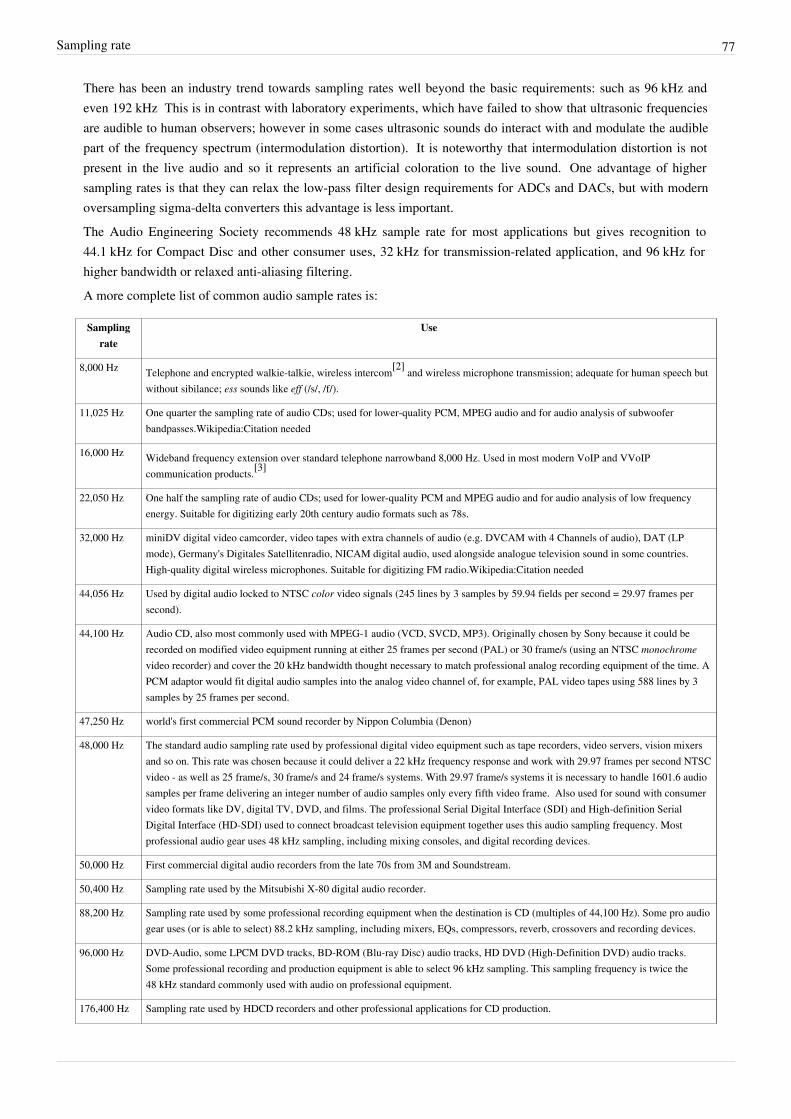
Sampling rate 77
There has been an industry trend towards sampling rates well beyond the basic requirements: such as 96 kHz andeven 192 kHz This is in contrast with laboratory experiments, which have failed to show that ultrasonic frequenciesare audible to human observers; however in some cases ultrasonic sounds do interact with and modulate the audiblepart of the frequency spectrum (intermodulation distortion). It is noteworthy that intermodulation distortion is notpresent in the live audio and so it represents an artificial coloration to the live sound. One advantage of highersampling rates is that they can relax the low-pass filter design requirements for ADCs and DACs, but with modernoversampling sigma-delta converters this advantage is less important.The Audio Engineering Society recommends 48 kHz sample rate for most applications but gives recognition to44.1 kHz for Compact Disc and other consumer uses, 32 kHz for transmission-related application, and 96 kHz forhigher bandwidth or relaxed anti-aliasing filtering.A more complete list of common audio sample rates is:
Samplingrate
Use
8,000 Hz Telephone and encrypted walkie-talkie, wireless intercom[2] and wireless microphone transmission; adequate for human speech butwithout sibilance; ess sounds like eff (/s/, /f/).
11,025 Hz One quarter the sampling rate of audio CDs; used for lower-quality PCM, MPEG audio and for audio analysis of subwooferbandpasses.Wikipedia:Citation needed
16,000 Hz Wideband frequency extension over standard telephone narrowband 8,000 Hz. Used in most modern VoIP and VVoIPcommunication products.[3]
22,050 Hz One half the sampling rate of audio CDs; used for lower-quality PCM and MPEG audio and for audio analysis of low frequencyenergy. Suitable for digitizing early 20th century audio formats such as 78s.
32,000 Hz miniDV digital video camcorder, video tapes with extra channels of audio (e.g. DVCAM with 4 Channels of audio), DAT (LPmode), Germany's Digitales Satellitenradio, NICAM digital audio, used alongside analogue television sound in some countries.High-quality digital wireless microphones. Suitable for digitizing FM radio.Wikipedia:Citation needed
44,056 Hz Used by digital audio locked to NTSC color video signals (245 lines by 3 samples by 59.94 fields per second = 29.97 frames persecond).
44,100 Hz Audio CD, also most commonly used with MPEG-1 audio (VCD, SVCD, MP3). Originally chosen by Sony because it could berecorded on modified video equipment running at either 25 frames per second (PAL) or 30 frame/s (using an NTSC monochromevideo recorder) and cover the 20 kHz bandwidth thought necessary to match professional analog recording equipment of the time. APCM adaptor would fit digital audio samples into the analog video channel of, for example, PAL video tapes using 588 lines by 3samples by 25 frames per second.
47,250 Hz world's first commercial PCM sound recorder by Nippon Columbia (Denon)
48,000 Hz The standard audio sampling rate used by professional digital video equipment such as tape recorders, video servers, vision mixersand so on. This rate was chosen because it could deliver a 22 kHz frequency response and work with 29.97 frames per second NTSCvideo - as well as 25 frame/s, 30 frame/s and 24 frame/s systems. With 29.97 frame/s systems it is necessary to handle 1601.6 audiosamples per frame delivering an integer number of audio samples only every fifth video frame. Also used for sound with consumervideo formats like DV, digital TV, DVD, and films. The professional Serial Digital Interface (SDI) and High-definition SerialDigital Interface (HD-SDI) used to connect broadcast television equipment together uses this audio sampling frequency. Mostprofessional audio gear uses 48 kHz sampling, including mixing consoles, and digital recording devices.
50,000 Hz First commercial digital audio recorders from the late 70s from 3M and Soundstream.
50,400 Hz Sampling rate used by the Mitsubishi X-80 digital audio recorder.
88,200 Hz Sampling rate used by some professional recording equipment when the destination is CD (multiples of 44,100 Hz). Some pro audiogear uses (or is able to select) 88.2 kHz sampling, including mixers, EQs, compressors, reverb, crossovers and recording devices.
96,000 Hz DVD-Audio, some LPCM DVD tracks, BD-ROM (Blu-ray Disc) audio tracks, HD DVD (High-Definition DVD) audio tracks.Some professional recording and production equipment is able to select 96 kHz sampling. This sampling frequency is twice the48 kHz standard commonly used with audio on professional equipment.
176,400 Hz Sampling rate used by HDCD recorders and other professional applications for CD production.
Sampling rate 78
192,000 Hz DVD-Audio, some LPCM DVD tracks, BD-ROM (Blu-ray Disc) audio tracks, and HD DVD (High-Definition DVD) audio tracks,High-Definition audio recording devices and audio editing software. This sampling frequency is four times the 48 kHz standardcommonly used with audio on professional video equipment.
352,800 Hz Digital eXtreme Definition, used for recording and editing Super Audio CDs, as 1-bit DSD is not suited for editing. Eight times thefrequency of 44.1 kHz.
2,822,400 Hz SACD, 1-bit delta-sigma modulation process known as Direct Stream Digital, co-developed by Sony and Philips.
5,644,800 Hz Double-Rate DSD, 1-bit Direct Stream Digital at 2x the rate of the SACD. Used in some professional DSD recorders.
Bit depth
See also: Audio bit depthAudio is typically recorded at 8-, 16-, and 20-bit depth, which yield a theoretical maximumSignal-to-quantization-noise ratio (SQNR) for a pure sine wave of, approximately, 49.93 dB, 98.09 dB and122.17 dB. CD quality audio uses 16-bit samples. Thermal noise limits the true number of bits that can be used inquantization. Few analog systems have signal to noise ratios (SNR) exceeding 120 dB. However, digital signalprocessing operations can have very high dynamic range, consequently it is common to perform mixing andmastering operations at 32-bit precision and then convert to 16 or 24 bit for distribution.
Speech sampling
Speech signals, i.e., signals intended to carry only human speech, can usually be sampled at a much lower rate. Formost phonemes, almost all of the energy is contained in the 5Hz-4 kHz range, allowing a sampling rate of 8 kHz.This is the sampling rate used by nearly all telephony systems, which use the G.711 sampling and quantizationspecifications.
Video samplingStandard-definition television (SDTV) uses either 720 by 480 pixels (US NTSC 525-line) or 704 by 576 pixels (UKPAL 625-line) for the visible picture area.High-definition television (HDTV) uses 720p (progressive), 1080i (interlaced), and 1080p (progressive, also knownas Full-HD).In digital video, the temporal sampling rate is defined the frame rate – or rather the field rate – rather than thenotional pixel clock. The image sampling frequency is the repetition rate of the sensor integration period. Since theintegration period may be significantly shorter than the time between repetitions, the sampling frequency can bedifferent from the inverse of the sample time:• 50 Hz – PAL video• 60 / 1.001 Hz ~= 59.94 Hz – NTSC videoVideo digital-to-analog converters operate in the megahertz range (from ~3 MHz for low quality composite videoscalers in early games consoles, to 250 MHz or more for the highest-resolution VGA output).When analog video is converted to digital video, a different sampling process occurs, this time at the pixelfrequency, corresponding to a spatial sampling rate along scan lines. A common pixel sampling rate is:• 13.5 MHz – CCIR 601, D1 videoSpatial sampling in the other direction is determined by the spacing of scan lines in the raster. The sampling ratesand resolutions in both spatial directions can be measured in units of lines per picture height.Spatial aliasing of high-frequency luma or chroma video components shows up as a moiré pattern.

Sampling rate 79
The top 2 graphs depict Fourier transforms of 2 different functions thatproduce the same results when sampled at a particular rate. The
baseband function is sampled faster than its Nyquist rate, and thebandpass function is undersampled, effectively converting it to
baseband. The lower graphs indicate how identical spectral results arecreated by the aliases of the sampling process.
3D sampling
• X-ray computed tomography uses 3 dimensionalspace
•• Voxel
Undersampling
Main article: UndersamplingWhen a bandpass signal is sampled slower than itsNyquist rate, the samples are indistinguishable fromsamples of a low-frequency alias of thehigh-frequency signal. That is often done purposefullyin such a way that the lowest-frequency alias satisfiesthe Nyquist criterion, because the bandpass signal isstill uniquely represented and recoverable. Suchundersampling is also known as bandpass sampling,harmonic sampling, IF sampling, and direct IF todigital conversion.
OversamplingMain article: OversamplingOversampling is used in most modern analog-to-digital converters to reduce the distortion introduced by practicaldigital-to-analog converters, such as a zero-order hold instead of idealizations like the Whittaker–Shannoninterpolation formula.
Complex samplingComplex sampling (I/Q sampling) refers to the simultaneous sampling of two different, but related, waveforms,resulting in pairs of samples that are subsequently treated as complex numbers.[4] When one waveform isthe Hilbert transform of the other waveform the complex-valued function,
is called an analytic signal, whose Fourier transform is zero for all negative values of frequency. In that case, theNyquist rate for a waveform with no frequencies ≥ B can be reduced to just B (complex samples/sec), instead of 2B(real samples/sec).[5] More apparently, the equivalent baseband waveform, also has a Nyquist
rate of B, because all of its non-zero frequency content is shifted into the interval [-B/2, B/2).Although complex-valued samples can be obtained as described above, they are also created by manipulatingsamples of a real-valued waveform. For instance, the equivalent baseband waveform can be created withoutexplicitly computing by processing the product sequence [6] through a digital
lowpass filter whose cutoff frequency is B/2.[7] Computing only every other sample of the output sequence reducesthe sample-rate commensurate with the reduced Nyquist rate. The result is half as many complex-valued samples asthe original number of real samples. No information is lost, and the original s(t) waveform can be recovered, ifnecessary.

Sampling rate 80
Notes[1] C. E. Shannon, "Communication in the presence of noise", Proc. Institute of Radio Engineers, vol. 37, no.1, pp. 10–21, Jan. 1949. Reprint as
classic paper in: Proc. IEEE, Vol. 86, No. 2, (Feb 1998) (http:/ / www. stanford. edu/ class/ ee104/ shannonpaper. pdf)[2] HME DX200 encrypted wireless intercom (http:/ / www. hme. com/ proDX200. cfm)[3] http:/ / www. voipsupply. com/ cisco-hd-voice[4] Sample-pairs are also sometimes viewed as points on a constellation diagram.[5] When the complex sample-rate is B, a frequency component at 0.6 B, for instance, will have an alias at −0.4 B, which is unambiguous
because of the constraint that the pre-sampled signal was analytic. Also see Aliasing#Complex_sinusoids[6][6] When s(t) is sampled at the Nyquist frequency (1/T = 2B), the product sequence simplifies to UNIQ-math-0-fdcc463dc40e329d-QINU[7][7] The sequence of complex numbers is convolved with the impulse response of a filter with real-valued coefficients. That is equivalent to
separately filtering the sequences of real parts and imaginary parts and reforming complex pairs at the outputs.
Citations
Further reading• Matt Pharr and Greg Humphreys, Physically Based Rendering: From Theory to Implementation, Morgan
Kaufmann, July 2004. ISBN 0-12-553180-X. The chapter on sampling ( available online (http:/ / graphics.stanford. edu/ ~mmp/ chapters/ pbrt_chapter7. pdf)) is nicely written with diagrams, core theory and code sample.
External links• Journal devoted to Sampling Theory (http:/ / www. stsip. org)• I/Q Data for Dummies (http:/ / whiteboard. ping. se/ SDR/ IQ) A page trying to answer the question Why I/Q
Data?
Nyquist–Shannon sampling theorem
Fig. 1: Fourier transform of a bandlimited function (amplitude vsfrequency)
In the field of digital signal processing, the samplingtheorem is a fundamental bridge between continuoussignals (analog domain) and discrete signals (digitaldomain). Strictly speaking, it only applies to a class ofmathematical functions whose Fourier transforms arezero outside of a finite region of frequencies (see Fig1). The analytical extension to actual signals, which canonly approximate that condition, is provided by thediscrete-time Fourier transform, a version of thePoisson summation formula. Intuitively we expect thatwhen one reduces a continuous function to a discretesequence (called samples) and interpolates back to a continuous function, the fidelity of the result depends on thedensity (or sample-rate) of the original samples. The sampling theorem introduces the concept of a sample-rate thatis sufficient for perfect fidelity for the class of bandlimited functions. And it expresses the sample-rate in terms ofthe function's bandwidth. Thus no actual "information" is lost during the sampling process. The theorem also leadsto a formula for the mathematically ideal interpolation algorithm.
The theorem does not preclude the possibility of perfect reconstruction under special circumstances that do notsatisfy the sample-rate criterion. (See Sampling of non-baseband signals below, and Compressed sensing.)The name Nyquist–Shannon sampling theorem honors Harry Nyquist and Claude Shannon. The theorem was also discovered independently by E. T. Whittaker, by Vladimir Kotelnikov, and by others. So it is also known by the

NyquistShannon sampling theorem 81
names Nyquist–Shannon–Kotelnikov, Whittaker–Shannon–Kotelnikov, Whittaker–Nyquist–Kotelnikov–Shannon,and cardinal theorem of interpolation.
IntroductionSampling is the process of converting a signal (for example, a function of continuous time or space) into a numericsequence (a function of discrete time or space). Shannon's version of the theorem states:[1]
If a function x(t) contains no frequencies higher than B hertz, it is completely determined by giving itsordinates at a series of points spaced 1/(2B) seconds apart.
A sufficient sample-rate is therefore samples/second, or anything larger. Conversely, for a given sample-rate the bandlimit for perfect reconstruction is When the bandlimit is too high (or there is no
bandlimit), the reconstruction exhibits imperfections known as aliasing. Modern statements of the theorem aresometimes careful to explicitly state that x(t) must contain no sinusoidal component at exactly frequency B, or that Bmust be strictly less than ½ the sample rate. The two thresholds, and are respectively called the Nyquistrate and Nyquist frequency. And respectively, they are attributes of x(t) and of the sampling equipment. Thecondition described by these inequalities is called the Nyquist criterion, or sometimes the Raabe condition. Thetheorem is also applicable to functions of other domains, such as space, in the case of a digitized image. The onlychange, in the case of other domains, is the units of measure applied to t, fs, and B.
Fig. 2: The normalized sinc function: sin(πx) / (πx) ... showing thecentral peak at x= 0, and zero-crossings at the other integer values of
x.
The symbol is customarily used torepresent the interval between samples. And thesamples of function x are denoted by x(nT), for allinteger values of n. The mathematically ideal way tointerpolate the sequence involves the use of sincfunctions, like those shown in Fig 2. Each sample in thesequence is replaced by a sinc function, centered on thetime axis at the original location of the sample (nT),with the amplitude of the sinc function scaled to thesample value, x(nT). Subsequently, the sinc functionsare summed into a continuous function. Amathematically equivalent method is to convolve onesinc function with a series of Dirac delta pulses,weighted by the sample values. Neither method isnumerically practical. Instead, some type ofapproximation of the sinc functions, finite in length, should be utilized. The imperfections attributable to theapproximation are known as interpolation error.
Practical digital-to-analog converters produce neither scaled and delayed sinc functions, nor ideal Dirac pulses.Instead they produce a piecewise-constant sequence of scaled and delayed rectangular pulses, usually followed by a"shaping filter" to clean up spurious high-frequency content.
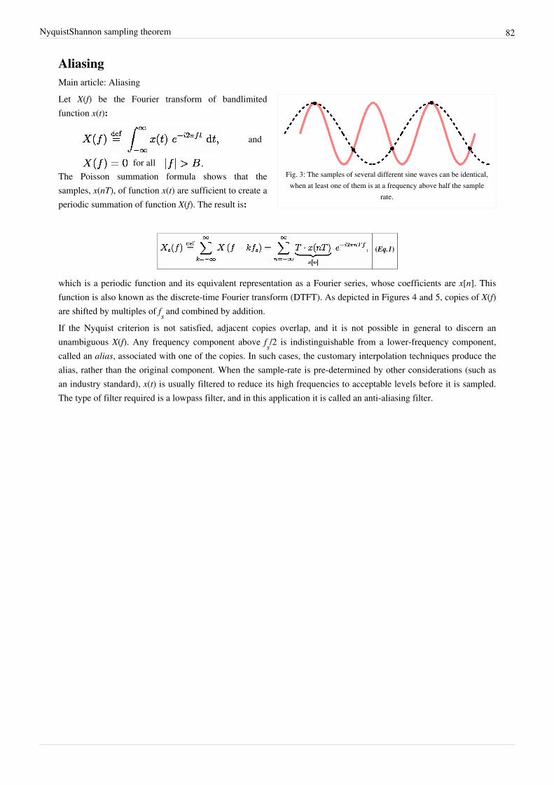
NyquistShannon sampling theorem 82
AliasingMain article: Aliasing
Fig. 3: The samples of several different sine waves can be identical,when at least one of them is at a frequency above half the sample
rate.
Let X(f) be the Fourier transform of bandlimitedfunction x(t):
and
for all The Poisson summation formula shows that thesamples, x(nT), of function x(t) are sufficient to create aperiodic summation of function X(f). The result is:
(Eq.1)
which is a periodic function and its equivalent representation as a Fourier series, whose coefficients are x[n]. Thisfunction is also known as the discrete-time Fourier transform (DTFT). As depicted in Figures 4 and 5, copies of X(f)are shifted by multiples of fs and combined by addition.If the Nyquist criterion is not satisfied, adjacent copies overlap, and it is not possible in general to discern anunambiguous X(f). Any frequency component above fs/2 is indistinguishable from a lower-frequency component,called an alias, associated with one of the copies. In such cases, the customary interpolation techniques produce thealias, rather than the original component. When the sample-rate is pre-determined by other considerations (such asan industry standard), x(t) is usually filtered to reduce its high frequencies to acceptable levels before it is sampled.The type of filter required is a lowpass filter, and in this application it is called an anti-aliasing filter.

NyquistShannon sampling theorem 83
Fig. 4: X(f) (top blue) and XA(f) (bottom blue) are continuous Fourier transforms of twodifferent functions, x(t) and xA(t) (not shown). When the functions are sampled at rate fs,
the images (green) are added to the original transforms (blue) when one examines thediscrete-time Fourier transforms (DTFT) of the sequences. In this hypothetical example,the DTFTs are identical, which means the sampled sequences are identical, even though
the original continuous pre-sampled functions are not. If these were audio signals, x(t) andxA(t) might not sound the same. But their samples (taken at rate fs) are identical and
would lead to identical reproduced sounds; thus xA(t) is an alias of x(t) at this sample rate.In this example (of a bandlimited function), such aliasing can be prevented by increasing
fs such that the green images in the top figure do not overlap the blue portion.
Fig. 5: Spectrum, Xs(f), of a properly sampled bandlimited signal (blue) and the adjacentDTFT images (green) that do not overlap. A brick-wall low-pass filter, H(f), removes the
images, leaves the original spectrum, X(f), and recovers the original signal from itssamples.
Derivation as a specialcase of Poissonsummation
From Figure 5, it is apparent that whenthere is no overlap of the copies (aka"images") of X(f), the k = 0 term ofXs(f) can be recovered by the product:
where:
At this point, the sampling theorem isproved, since X(f) uniquely determinesx(t).
All that remains is to derive theformula for reconstruction. H(f) neednot be precisely defined in the region[B, fs − B] because Xs(f) is zero in thatregion. However, the worst case iswhen B = fs/2, the Nyquist frequency.A function that is sufficient for thatand all less severe cases is:
where rect(•) is the rectangularfunction. Therefore:
(from Eq.1, above).
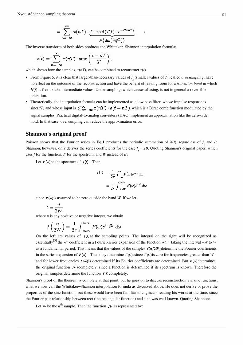
NyquistShannon sampling theorem 84
[2]
The inverse transform of both sides produces the Whittaker–Shannon interpolation formula:
which shows how the samples, x(nT), can be combined to reconstruct x(t).• From Figure 5, it is clear that larger-than-necessary values of fs (smaller values of T), called oversampling, have
no effect on the outcome of the reconstruction and have the benefit of leaving room for a transition band in whichH(f) is free to take intermediate values. Undersampling, which causes aliasing, is not in general a reversibleoperation.
• Theoretically, the interpolation formula can be implemented as a low pass filter, whose impulse response issinc(t/T) and whose input is which is a Dirac comb function modulated by thesignal samples. Practical digital-to-analog converters (DAC) implement an approximation like the zero-orderhold. In that case, oversampling can reduce the approximation error.
Shannon's original proofPoisson shows that the Fourier series in Eq.1 produces the periodic summation of X(f), regardless of fs and B.Shannon, however, only derives the series coefficients for the case fs = 2B. Quoting Shannon's original paper, whichuses f for the function, F for the spectrum, and W instead of B:
Let be the spectrum of Then
since is assumed to be zero outside the band W. If we let
where n is any positive or negative integer, we obtain
On the left are values of at the sampling points. The integral on the right will be recognized asessentially[3] the nth coefficient in a Fourier-series expansion of the function taking the interval –W to Was a fundamental period. This means that the values of the samples determine the Fourier coefficientsin the series expansion of Thus they determine since is zero for frequencies greater than W,and for lower frequencies is determined if its Fourier coefficients are determined. But determinesthe original function completely, since a function is determined if its spectrum is known. Therefore theoriginal samples determine the function completely.
Shannon's proof of the theorem is complete at that point, but he goes on to discuss reconstruction via sinc functions,what we now call the Whittaker–Shannon interpolation formula as discussed above. He does not derive or prove theproperties of the sinc function, but these would have been familiar to engineers reading his works at the time, sincethe Fourier pair relationship between rect (the rectangular function) and sinc was well known. Quoting Shannon:
Let be the nth sample. Then the function is represented by:
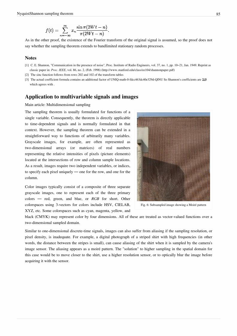
NyquistShannon sampling theorem 85
As in the other proof, the existence of the Fourier transform of the original signal is assumed, so the proof does notsay whether the sampling theorem extends to bandlimited stationary random processes.
Notes[1] C. E. Shannon, "Communication in the presence of noise", Proc. Institute of Radio Engineers, vol. 37, no. 1, pp. 10–21, Jan. 1949. Reprint as
classic paper in: Proc. IEEE, vol. 86, no. 2, (Feb. 1998) (http:/ / www. stanford. edu/ class/ ee104/ shannonpaper. pdf)[2] The sinc function follows from rows 202 and 102 of the transform tables[3] The actual coefficient formula contains an additional factor of UNIQ-math-0-fdcc463dc40e329d-QINU So Shannon's coefficients are
which agrees with .
Application to multivariable signals and imagesMain article: Multidimensional sampling
Fig. 6: Subsampled image showing a Moiré pattern
The sampling theorem is usually formulated for functions of asingle variable. Consequently, the theorem is directly applicableto time-dependent signals and is normally formulated in thatcontext. However, the sampling theorem can be extended in astraightforward way to functions of arbitrarily many variables.Grayscale images, for example, are often represented astwo-dimensional arrays (or matrices) of real numbersrepresenting the relative intensities of pixels (picture elements)located at the intersections of row and column sample locations.As a result, images require two independent variables, or indices,to specify each pixel uniquely — one for the row, and one for thecolumn.
Color images typically consist of a composite of three separategrayscale images, one to represent each of the three primarycolors — red, green, and blue, or RGB for short. Othercolorspaces using 3-vectors for colors include HSV, CIELAB,XYZ, etc. Some colorspaces such as cyan, magenta, yellow, andblack (CMYK) may represent color by four dimensions. All of these are treated as vector-valued functions over atwo-dimensional sampled domain.
Similar to one-dimensional discrete-time signals, images can also suffer from aliasing if the sampling resolution, orpixel density, is inadequate. For example, a digital photograph of a striped shirt with high frequencies (in otherwords, the distance between the stripes is small), can cause aliasing of the shirt when it is sampled by the camera'simage sensor. The aliasing appears as a moiré pattern. The "solution" to higher sampling in the spatial domain forthis case would be to move closer to the shirt, use a higher resolution sensor, or to optically blur the image beforeacquiring it with the sensor.
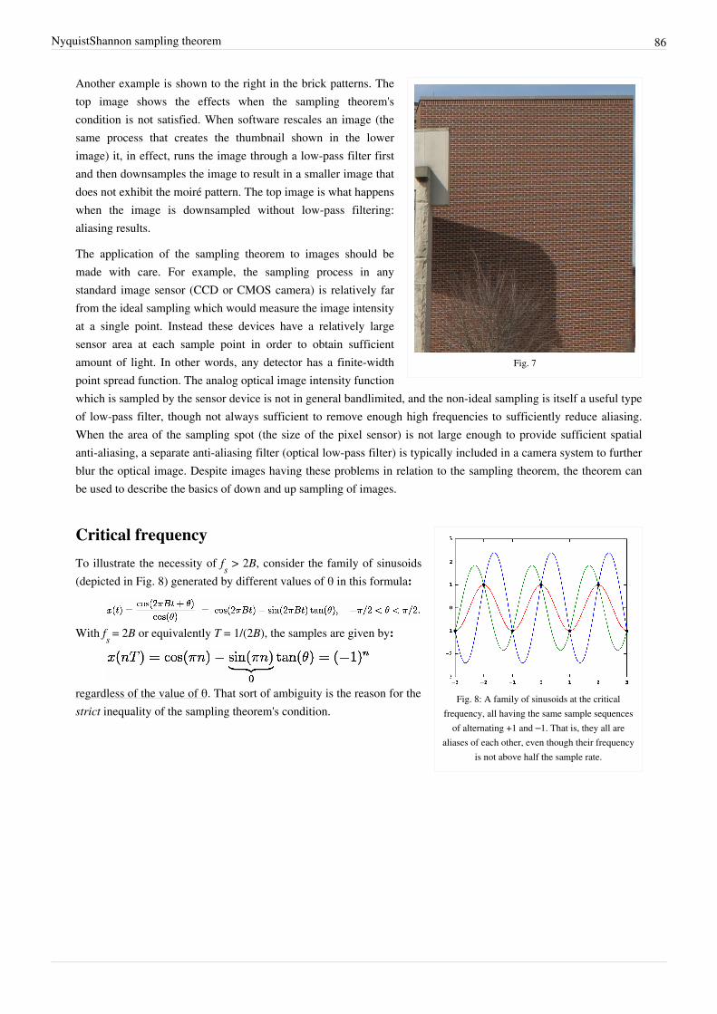
NyquistShannon sampling theorem 86
Fig. 7
Another example is shown to the right in the brick patterns. Thetop image shows the effects when the sampling theorem'scondition is not satisfied. When software rescales an image (thesame process that creates the thumbnail shown in the lowerimage) it, in effect, runs the image through a low-pass filter firstand then downsamples the image to result in a smaller image thatdoes not exhibit the moiré pattern. The top image is what happenswhen the image is downsampled without low-pass filtering:aliasing results.
The application of the sampling theorem to images should bemade with care. For example, the sampling process in anystandard image sensor (CCD or CMOS camera) is relatively farfrom the ideal sampling which would measure the image intensityat a single point. Instead these devices have a relatively largesensor area at each sample point in order to obtain sufficientamount of light. In other words, any detector has a finite-widthpoint spread function. The analog optical image intensity functionwhich is sampled by the sensor device is not in general bandlimited, and the non-ideal sampling is itself a useful typeof low-pass filter, though not always sufficient to remove enough high frequencies to sufficiently reduce aliasing.When the area of the sampling spot (the size of the pixel sensor) is not large enough to provide sufficient spatialanti-aliasing, a separate anti-aliasing filter (optical low-pass filter) is typically included in a camera system to furtherblur the optical image. Despite images having these problems in relation to the sampling theorem, the theorem canbe used to describe the basics of down and up sampling of images.
Fig. 8: A family of sinusoids at the criticalfrequency, all having the same sample sequences
of alternating +1 and –1. That is, they all arealiases of each other, even though their frequency
is not above half the sample rate.
Critical frequency
To illustrate the necessity of fs > 2B, consider the family of sinusoids(depicted in Fig. 8) generated by different values of θ in this formula:
With fs = 2B or equivalently T = 1/(2B), the samples are given by:
regardless of the value of θ. That sort of ambiguity is the reason for thestrict inequality of the sampling theorem's condition.
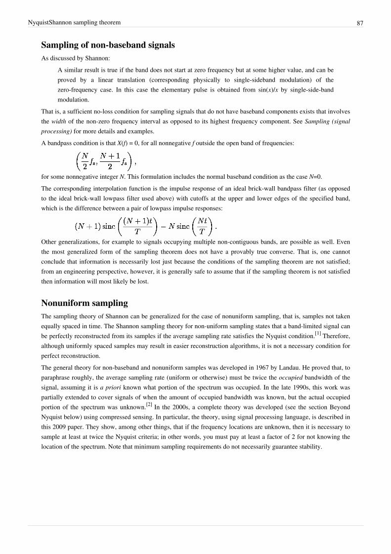
NyquistShannon sampling theorem 87
Sampling of non-baseband signalsAs discussed by Shannon:
A similar result is true if the band does not start at zero frequency but at some higher value, and can beproved by a linear translation (corresponding physically to single-sideband modulation) of thezero-frequency case. In this case the elementary pulse is obtained from sin(x)/x by single-side-bandmodulation.
That is, a sufficient no-loss condition for sampling signals that do not have baseband components exists that involvesthe width of the non-zero frequency interval as opposed to its highest frequency component. See Sampling (signalprocessing) for more details and examples.A bandpass condition is that X(f) = 0, for all nonnegative f outside the open band of frequencies:
for some nonnegative integer N. This formulation includes the normal baseband condition as the case N=0.The corresponding interpolation function is the impulse response of an ideal brick-wall bandpass filter (as opposedto the ideal brick-wall lowpass filter used above) with cutoffs at the upper and lower edges of the specified band,which is the difference between a pair of lowpass impulse responses:
Other generalizations, for example to signals occupying multiple non-contiguous bands, are possible as well. Eventhe most generalized form of the sampling theorem does not have a provably true converse. That is, one cannotconclude that information is necessarily lost just because the conditions of the sampling theorem are not satisfied;from an engineering perspective, however, it is generally safe to assume that if the sampling theorem is not satisfiedthen information will most likely be lost.
Nonuniform samplingThe sampling theory of Shannon can be generalized for the case of nonuniform sampling, that is, samples not takenequally spaced in time. The Shannon sampling theory for non-uniform sampling states that a band-limited signal canbe perfectly reconstructed from its samples if the average sampling rate satisfies the Nyquist condition.[1] Therefore,although uniformly spaced samples may result in easier reconstruction algorithms, it is not a necessary condition forperfect reconstruction.The general theory for non-baseband and nonuniform samples was developed in 1967 by Landau. He proved that, toparaphrase roughly, the average sampling rate (uniform or otherwise) must be twice the occupied bandwidth of thesignal, assuming it is a priori known what portion of the spectrum was occupied. In the late 1990s, this work waspartially extended to cover signals of when the amount of occupied bandwidth was known, but the actual occupiedportion of the spectrum was unknown.[2] In the 2000s, a complete theory was developed (see the section BeyondNyquist below) using compressed sensing. In particular, the theory, using signal processing language, is described inthis 2009 paper. They show, among other things, that if the frequency locations are unknown, then it is necessary tosample at least at twice the Nyquist criteria; in other words, you must pay at least a factor of 2 for not knowing thelocation of the spectrum. Note that minimum sampling requirements do not necessarily guarantee stability.
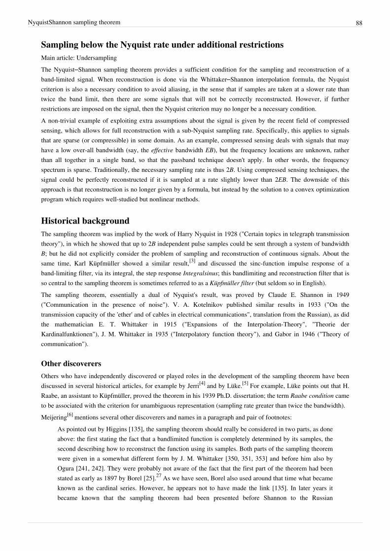
NyquistShannon sampling theorem 88
Sampling below the Nyquist rate under additional restrictionsMain article: UndersamplingThe Nyquist–Shannon sampling theorem provides a sufficient condition for the sampling and reconstruction of aband-limited signal. When reconstruction is done via the Whittaker–Shannon interpolation formula, the Nyquistcriterion is also a necessary condition to avoid aliasing, in the sense that if samples are taken at a slower rate thantwice the band limit, then there are some signals that will not be correctly reconstructed. However, if furtherrestrictions are imposed on the signal, then the Nyquist criterion may no longer be a necessary condition.A non-trivial example of exploiting extra assumptions about the signal is given by the recent field of compressedsensing, which allows for full reconstruction with a sub-Nyquist sampling rate. Specifically, this applies to signalsthat are sparse (or compressible) in some domain. As an example, compressed sensing deals with signals that mayhave a low over-all bandwidth (say, the effective bandwidth EB), but the frequency locations are unknown, ratherthan all together in a single band, so that the passband technique doesn't apply. In other words, the frequencyspectrum is sparse. Traditionally, the necessary sampling rate is thus 2B. Using compressed sensing techniques, thesignal could be perfectly reconstructed if it is sampled at a rate slightly lower than 2EB. The downside of thisapproach is that reconstruction is no longer given by a formula, but instead by the solution to a convex optimizationprogram which requires well-studied but nonlinear methods.
Historical backgroundThe sampling theorem was implied by the work of Harry Nyquist in 1928 ("Certain topics in telegraph transmissiontheory"), in which he showed that up to 2B independent pulse samples could be sent through a system of bandwidthB; but he did not explicitly consider the problem of sampling and reconstruction of continuous signals. About thesame time, Karl Küpfmüller showed a similar result,[3] and discussed the sinc-function impulse response of aband-limiting filter, via its integral, the step response Integralsinus; this bandlimiting and reconstruction filter that isso central to the sampling theorem is sometimes referred to as a Küpfmüller filter (but seldom so in English).The sampling theorem, essentially a dual of Nyquist's result, was proved by Claude E. Shannon in 1949("Communication in the presence of noise"). V. A. Kotelnikov published similar results in 1933 ("On thetransmission capacity of the 'ether' and of cables in electrical communications", translation from the Russian), as didthe mathematician E. T. Whittaker in 1915 ("Expansions of the Interpolation-Theory", "Theorie derKardinalfunktionen"), J. M. Whittaker in 1935 ("Interpolatory function theory"), and Gabor in 1946 ("Theory ofcommunication").
Other discoverersOthers who have independently discovered or played roles in the development of the sampling theorem have beendiscussed in several historical articles, for example by Jerri[4] and by Lüke.[5] For example, Lüke points out that H.Raabe, an assistant to Küpfmüller, proved the theorem in his 1939 Ph.D. dissertation; the term Raabe condition cameto be associated with the criterion for unambiguous representation (sampling rate greater than twice the bandwidth).Meijering[6] mentions several other discoverers and names in a paragraph and pair of footnotes:
As pointed out by Higgins [135], the sampling theorem should really be considered in two parts, as done above: the first stating the fact that a bandlimited function is completely determined by its samples, the second describing how to reconstruct the function using its samples. Both parts of the sampling theorem were given in a somewhat different form by J. M. Whittaker [350, 351, 353] and before him also by Ogura [241, 242]. They were probably not aware of the fact that the first part of the theorem had been stated as early as 1897 by Borel [25].27 As we have seen, Borel also used around that time what became known as the cardinal series. However, he appears not to have made the link [135]. In later years it became known that the sampling theorem had been presented before Shannon to the Russian

NyquistShannon sampling theorem 89
communication community by Kotel'nikov [173]. In more implicit, verbal form, it had also beendescribed in the German literature by Raabe [257]. Several authors [33, 205] have mentioned thatSomeya [296] introduced the theorem in the Japanese literature parallel to Shannon. In the Englishliterature, Weston [347] introduced it independently of Shannon around the same time.28
27 Several authors, following Black [16], have claimed that this first part of the sampling theorem wasstated even earlier by Cauchy, in a paper [41] published in 1841. However, the paper of Cauchy does notcontain such a statement, as has been pointed out by Higgins [135].28 As a consequence of the discovery of the several independent introductions of the sampling theorem,people started to refer to the theorem by including the names of the aforementioned authors, resulting insuch catchphrases as “the Whittaker-Kotel’nikov-Shannon (WKS) sampling theorem" [155] or even "theWhittaker-Kotel'nikov-Raabe-Shannon-Someya sampling theorem" [33]. To avoid confusion, perhapsthe best thing to do is to refer to it as the sampling theorem, "rather than trying to find a title that doesjustice to all claimants" [136].
Why Nyquist?Exactly how, when, or why Harry Nyquist had his name attached to the sampling theorem remains obscure. The termNyquist Sampling Theorem (capitalized thus) appeared as early as 1959 in a book from his former employer, BellLabs, and appeared again in 1963, and not capitalized in 1965. It had been called the Shannon Sampling Theorem asearly as 1954, but also just the sampling theorem by several other books in the early 1950s.In 1958, Blackman and Tukey cited Nyquist's 1928 paper as a reference for the sampling theorem of informationtheory, even though that paper does not treat sampling and reconstruction of continuous signals as others did. Theirglossary of terms includes these entries:
Sampling theorem (of information theory)Nyquist's result that equi-spaced data, with two or more points per cycle of highest frequency, allowsreconstruction of band-limited functions. (See Cardinal theorem.)Cardinal theorem (of interpolation theory)A precise statement of the conditions under which values given at a doubly infinite set of equally spacedpoints can be interpolated to yield a continuous band-limited function with the aid of the function
Exactly what "Nyquist's result" they are referring to remains mysterious.When Shannon stated and proved the sampling theorem in his 1949 paper, according to Meijering "he referred to thecritical sampling interval T = 1/(2W) as the Nyquist interval corresponding to the band W, in recognition of Nyquist’sdiscovery of the fundamental importance of this interval in connection with telegraphy." This explains Nyquist'sname on the critical interval, but not on the theorem.Similarly, Nyquist's name was attached to Nyquist rate in 1953 by Harold S. Black:
"If the essential frequency range is limited to B cycles per second, 2B was given by Nyquist as the maximumnumber of code elements per second that could be unambiguously resolved, assuming the peak interference isless half a quantum step. This rate is generally referred to as signaling at the Nyquist rate and 1/(2B) hasbeen termed a Nyquist interval." (bold added for emphasis; italics as in the original)
According to the OED, this may be the origin of the term Nyquist rate. In Black's usage, it is not a sampling rate, buta signaling rate.

NyquistShannon sampling theorem 90
Notes[1][1] Nonuniform Sampling, Theory and Practice (ed. F. Marvasti), Kluwer Academic/Plenum Publishers, New York, 2000[2][2] see, e.g.,[3] (English translation 2005) (http:/ / ict. open. ac. uk/ classics/ 2. pdf).[4] Abdul Jerri, The Shannon Sampling Theorem—Its Various Extensions and Applications: A Tutorial Review (http:/ / web. archive. org/ web/
20080605171238/ http:/ / ieeexplore. ieee. org/ search/ wrapper. jsp?arnumber=1455040), Proceedings of the IEEE, 65:1565–1595, Nov.1977. See also Correction to "The Shannon sampling theorem—Its various extensions and applications: A tutorial review" (http:/ / web.archive. org/ web/ 20090120203809/ http:/ / ieeexplore. ieee. org/ search/ wrapper. jsp?arnumber=1455576), Proceedings of the IEEE, 67:695,April 1979
[5] Hans Dieter Lüke, , IEEE Communications Magazine, pp.106–108, April 1999.[6] Erik Meijering, , Proc. IEEE, 90, 2002.
References• J. R. Higgins: Five short stories about the cardinal series, Bulletin of the AMS 12(1985)• V. A. Kotelnikov, "On the carrying capacity of the ether and wire in telecommunications", Material for the First
All-Union Conference on Questions of Communication, Izd. Red. Upr. Svyazi RKKA, Moscow, 1933 (Russian).(english translation, PDF) (http:/ / ict. open. ac. uk/ classics/ 1. pdf)
• Karl Küpfmüller, "Utjämningsförlopp inom Telegraf- och Telefontekniken", ("Transients in telegraph andtelephone engineering"), Teknisk Tidskrift, no. 9 pp. 153–160 and 10 pp. 178–182, 1931. (http:/ / runeberg. org/tektid/ 1931e/ 0157. html) (http:/ / runeberg. org/ tektid/ 1931e/ 0182. html)
• R.J. Marks II: Introduction to Shannon Sampling and Interpolation Theory (http:/ / marksmannet. com/RobertMarks/ REPRINTS/ 1999_IntroductionToShannonSamplingAndInterpolationTheory. pdf),Spinger-Verlag, 1991.
• R.J. Marks II, Editor: Advanced Topics in Shannon Sampling and Interpolation Theory (http:/ / marksmannet.com/ RobertMarks/ REPRINTS/ 1993_AdvancedTopicsOnShannon. pdf), Springer-Verlag, 1993.
• R.J. Marks II, Handbook of Fourier Analysis and Its Applications, Oxford University Press, (2009), Chapters 5-8.Google books (http:/ / books. google. com/ books?id=Sp7O4bocjPAC).
• H. Nyquist, "Certain topics in telegraph transmission theory", Trans. AIEE, vol. 47, pp. 617–644, Apr. 1928Reprint as classic paper in: Proc. IEEE, Vol. 90, No. 2, Feb 2002 (http:/ / replay. web. archive. org/20060706192816/ http:/ / www. loe. ee. upatras. gr/ Comes/ Notes/ Nyquist. pdf).
• Press, WH; Teukolsky, SA; Vetterling, WT; Flannery, BP (2007), "Section 13.11. Numerical Use of the SamplingTheorem" (http:/ / apps. nrbook. com/ empanel/ index. html#pg=717), Numerical Recipes: The Art of ScientificComputing (3rd ed.), New York: Cambridge University Press, ISBN 978-0-521-88068-8
• C. E. Shannon, "Communication in the presence of noise", Proc. Institute of Radio Engineers, vol. 37, no.1,pp. 10–21, Jan. 1949. Reprint as classic paper in: Proc. IEEE, Vol. 86, No. 2, (Feb 1998) (http:/ / www. stanford.edu/ class/ ee104/ shannonpaper. pdf)
• Michael Unser: Sampling-50 Years after Shannon (http:/ / bigwww. epfl. ch/ publications/ unser0001. html), Proc.IEEE, vol. 88, no. 4, pp. 569–587, April 2000
• E. T. Whittaker, "On the Functions Which are Represented by the Expansions of the Interpolation Theory", Proc.Royal Soc. Edinburgh, Sec. A, vol.35, pp. 181–194, 1915
• J. M. Whittaker, Interpolatory Function Theory, Cambridge Univ. Press, Cambridge, England, 1935.

NyquistShannon sampling theorem 91
External links• Learning by Simulations (http:/ / www. vias. org/ simulations/ simusoft_nykvist. html) Interactive simulation of
the effects of inadequate sampling• Undersampling and an application of it (http:/ / spazioscuola. altervista. org/ UndersamplingAR/
UndersamplingARnv. htm)• Sampling Theory For Digital Audio (http:/ / web. archive. org/ web/ 20060614125302/ http:/ / www.
lavryengineering. com/ documents/ Sampling_Theory. pdf)• Journal devoted to Sampling Theory (http:/ / www. stsip. org/ )• Sampling Theorem with Constant Amplitude Variable Width Pulse (http:/ / ieeexplore. ieee. org/ xpl/ login.
jsp?tp=& arnumber=5699377& url=http:/ / ieeexplore. ieee. org/ xpls/ abs_all. jsp?arnumber=5699377)• "The Origins of the Sampling Theorem" by Hans Dieter Lüke published in "IEEE Communications Magazine"
April 1999. CiteSeerX: 10.1.1.163.2887 (http:/ / citeseerx. ist. psu. edu/ viewdoc/ summary?doi=10. 1. 1. 163.2887).
Nyquist frequencyNot to be confused with Nyquist rate.
Fig 1. The black dots are aliases of each other. The solid red line is an example ofadjusting amplitude vs frequency. The dashed red lines are the corresponding paths of the
aliases.
The Nyquist frequency, named afterelectronic engineer Harry Nyquist, is ½of the sampling rate of a discrete signalprocessing system. It is sometimesknown as the folding frequency of asampling system. An example offolding is depicted in Figure 1, wherefs is the sampling rate and 0.5 fs is thecorresponding Nyquist frequency. Theblack dot plotted at 0.6 fs representsthe amplitude and frequency of asinusoidal function whose frequency is60% of the sample-rate (fs). The otherthree dots indicate the frequencies and amplitudes of three other sinusoids that would produce the same set ofsamples as the actual sinusoid that was sampled. The symmetry about 0.5 fs is referred to as folding.
The Nyquist frequency should not be confused with the Nyquist rate, which is the minimum sampling rate thatsatisfies the Nyquist sampling criterion for a given signal or family of signals. The Nyquist rate is twice themaximum component frequency of the function being sampled. For example, the Nyquist rate for the sinusoid at0.6 fs is 1.2 fs, which means that at the fs rate, it is being undersampled. Thus, Nyquist rate is a property of acontinuous-time signal, whereas Nyquist frequency is a property of a discrete-time system.When the function domain is time, sample rates are usually expressed in samples/second, and the unit of Nyquistfrequency is cycles/second (hertz). When the function domain is distance, as in an image sampling system, thesample rate might be dots per inch and the corresponding Nyquist frequency would be in cycles/inch.

Nyquist frequency 92
AliasingMain article: AliasingReferring again to Figure 1, undersampling of the sinusoid at 0.6 fs is what allows there to be a lower-frequencyalias, which is a different function that produces the same set of samples. That condition is usually described asaliasing. The mathematical algorithms that are typically used to recreate a continuous function from its samples willmisinterpret the contributions of undersampled frequency components, which causes distortion. Samples of a pure0.6 fs sinusoid would produce a 0.4 fs sinusoid instead. If the true frequency was 0.4 fs, there would still be aliases at0.6, 1.4, 1.6, etc.,Wikipedia:Vagueness but the reconstructed frequency would be correct.In a typical application of sampling, one first chooses the highest frequency to be preserved and recreated, based onthe expected content (voice, music, etc.) and desired fidelity. Then one inserts an anti-aliasing filter ahead of thesampler. Its job is to attenuate the frequencies above that limit. Finally, based on the characteristics of the filter, onechooses a sample-rate (and corresponding Nyquist frequency) that will provide an acceptably small amount ofaliasing.In applications where the sample-rate is pre-determined, the filter is chosen based on the Nyquist frequency, ratherthan vice-versa. For example, audio CDs have a sampling rate of 44100 samples/sec. The Nyquist frequency istherefore 22050 Hz. The anti-aliasing filter must adequately suppress any higher frequencies but negligibly affect thefrequencies within the human hearing range. A filter that preserves 0–20 kHz is more than adequate for that.
Other meaningsEarly uses of the term Nyquist frequency, such as those cited above, are all consistent with the definition presented inthis article. Some later publications, including some respectable textbooks, call twice the signal bandwidth theNyquist frequency; this is a distinctly minority usage, and the frequency at twice the signal bandwidth is otherwisecommonly referred to as the Nyquist rate.
References
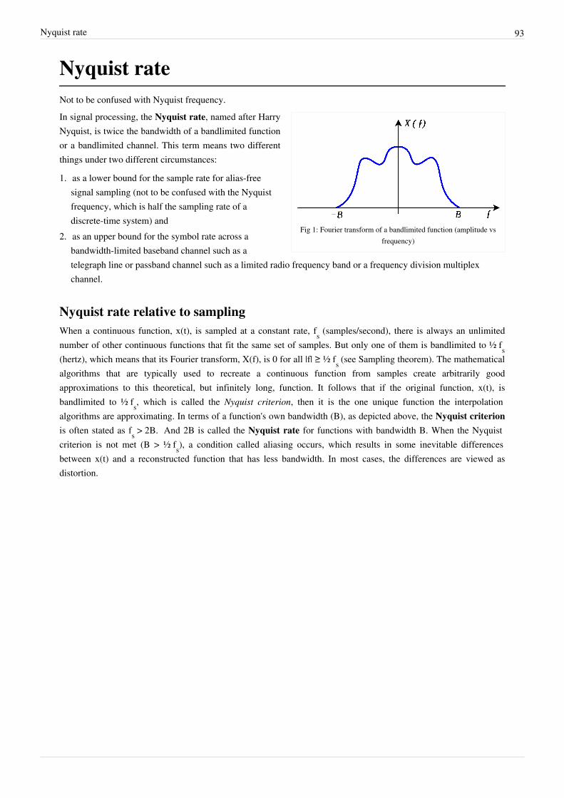
Nyquist rate 93
Nyquist rateNot to be confused with Nyquist frequency.
Fig 1: Fourier transform of a bandlimited function (amplitude vsfrequency)
In signal processing, the Nyquist rate, named after HarryNyquist, is twice the bandwidth of a bandlimited functionor a bandlimited channel. This term means two differentthings under two different circumstances:
1. as a lower bound for the sample rate for alias-freesignal sampling (not to be confused with the Nyquistfrequency, which is half the sampling rate of adiscrete-time system) and
2. as an upper bound for the symbol rate across abandwidth-limited baseband channel such as atelegraph line or passband channel such as a limited radio frequency band or a frequency division multiplexchannel.
Nyquist rate relative to samplingWhen a continuous function, x(t), is sampled at a constant rate, fs (samples/second), there is always an unlimitednumber of other continuous functions that fit the same set of samples. But only one of them is bandlimited to ½ fs(hertz), which means that its Fourier transform, X(f), is 0 for all |f| ≥ ½ fs (see Sampling theorem). The mathematicalalgorithms that are typically used to recreate a continuous function from samples create arbitrarily goodapproximations to this theoretical, but infinitely long, function. It follows that if the original function, x(t), isbandlimited to ½ fs, which is called the Nyquist criterion, then it is the one unique function the interpolationalgorithms are approximating. In terms of a function's own bandwidth (B), as depicted above, the Nyquist criterionis often stated as fs > 2B. And 2B is called the Nyquist rate for functions with bandwidth B. When the Nyquistcriterion is not met (B > ½ fs), a condition called aliasing occurs, which results in some inevitable differencesbetween x(t) and a reconstructed function that has less bandwidth. In most cases, the differences are viewed asdistortion.
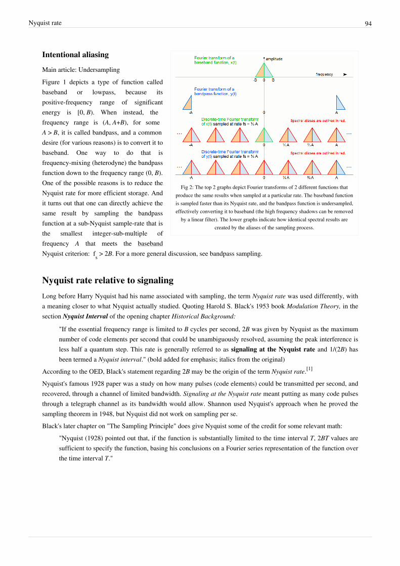
Nyquist rate 94
Fig 2: The top 2 graphs depict Fourier transforms of 2 different functions thatproduce the same results when sampled at a particular rate. The baseband functionis sampled faster than its Nyquist rate, and the bandpass function is undersampled,effectively converting it to baseband (the high frequency shadows can be removed
by a linear filter). The lower graphs indicate how identical spectral results arecreated by the aliases of the sampling process.
Intentional aliasing
Main article: UndersamplingFigure 1 depicts a type of function calledbaseband or lowpass, because itspositive-frequency range of significantenergy is [0, B). When instead, thefrequency range is (A, A+B), for someA > B, it is called bandpass, and a commondesire (for various reasons) is to convert it tobaseband. One way to do that isfrequency-mixing (heterodyne) the bandpassfunction down to the frequency range (0, B).One of the possible reasons is to reduce theNyquist rate for more efficient storage. Andit turns out that one can directly achieve thesame result by sampling the bandpassfunction at a sub-Nyquist sample-rate that isthe smallest integer-sub-multiple offrequency A that meets the basebandNyquist criterion: fs > 2B. For a more general discussion, see bandpass sampling.
Nyquist rate relative to signaling
Long before Harry Nyquist had his name associated with sampling, the term Nyquist rate was used differently, witha meaning closer to what Nyquist actually studied. Quoting Harold S. Black's 1953 book Modulation Theory, in thesection Nyquist Interval of the opening chapter Historical Background:
"If the essential frequency range is limited to B cycles per second, 2B was given by Nyquist as the maximumnumber of code elements per second that could be unambiguously resolved, assuming the peak interference isless half a quantum step. This rate is generally referred to as signaling at the Nyquist rate and 1/(2B) hasbeen termed a Nyquist interval." (bold added for emphasis; italics from the original)
According to the OED, Black's statement regarding 2B may be the origin of the term Nyquist rate.[1]
Nyquist's famous 1928 paper was a study on how many pulses (code elements) could be transmitted per second, andrecovered, through a channel of limited bandwidth. Signaling at the Nyquist rate meant putting as many code pulsesthrough a telegraph channel as its bandwidth would allow. Shannon used Nyquist's approach when he proved thesampling theorem in 1948, but Nyquist did not work on sampling per se.Black's later chapter on "The Sampling Principle" does give Nyquist some of the credit for some relevant math:
"Nyquist (1928) pointed out that, if the function is substantially limited to the time interval T, 2BT values aresufficient to specify the function, basing his conclusions on a Fourier series representation of the function overthe time interval T."
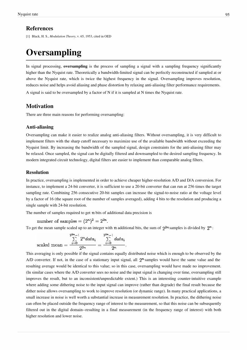
Nyquist rate 95
References[1] Black, H. S., Modulation Theory, v. 65, 1953, cited in OED
OversamplingIn signal processing, oversampling is the process of sampling a signal with a sampling frequency significantlyhigher than the Nyquist rate. Theoretically a bandwidth-limited signal can be perfectly reconstructed if sampled at orabove the Nyquist rate, which is twice the highest frequency in the signal. Oversampling improves resolution,reduces noise and helps avoid aliasing and phase distortion by relaxing anti-aliasing filter performance requirements.A signal is said to be oversampled by a factor of N if it is sampled at N times the Nyquist rate.
MotivationThere are three main reasons for performing oversampling:
Anti-aliasingOversampling can make it easier to realize analog anti-aliasing filters. Without oversampling, it is very difficult toimplement filters with the sharp cutoff necessary to maximize use of the available bandwidth without exceeding theNyquist limit. By increasing the bandwidth of the sampled signal, design constraints for the anti-aliasing filter maybe relaxed. Once sampled, the signal can be digitally filtered and downsampled to the desired sampling frequency. Inmodern integrated circuit technology, digital filters are easier to implement than comparable analog filters.
ResolutionIn practice, oversampling is implemented in order to achieve cheaper higher-resolution A/D and D/A conversion. Forinstance, to implement a 24-bit converter, it is sufficient to use a 20-bit converter that can run at 256 times the targetsampling rate. Combining 256 consecutive 20-bit samples can increase the signal-to-noise ratio at the voltage levelby a factor of 16 (the square root of the number of samples averaged), adding 4 bits to the resolution and producing asingle sample with 24-bit resolution.The number of samples required to get bits of additional data precision is
To get the mean sample scaled up to an integer with additional bits, the sum of samples is divided by :
This averaging is only possible if the signal contains equally distributed noise which is enough to be observed by theA/D converter. If not, in the case of a stationary input signal, all samples would have the same value and theresulting average would be identical to this value; so in this case, oversampling would have made no improvement.(In similar cases where the A/D converter sees no noise and the input signal is changing over time, oversampling stillimproves the result, but to an inconsistent/unpredictable extent.) This is an interesting counter-intuitive examplewhere adding some dithering noise to the input signal can improve (rather than degrade) the final result because thedither noise allows oversampling to work to improve resolution (or dynamic range). In many practical applications, asmall increase in noise is well worth a substantial increase in measurement resolution. In practice, the dithering noisecan often be placed outside the frequency range of interest to the measurement, so that this noise can be subsequentlyfiltered out in the digital domain--resulting in a final measurement (in the frequency range of interest) with bothhigher resolution and lower noise.
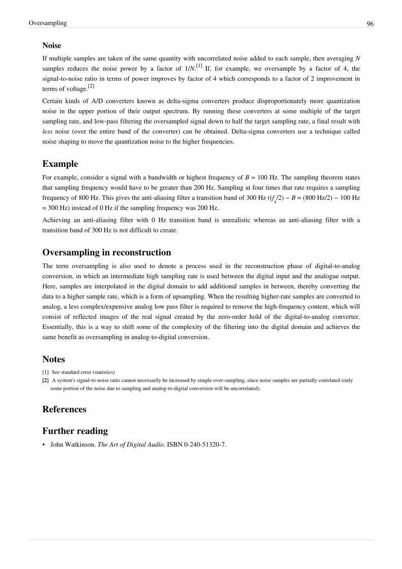
Oversampling 96
NoiseIf multiple samples are taken of the same quantity with uncorrelated noise added to each sample, then averaging Nsamples reduces the noise power by a factor of 1/N.[1] If, for example, we oversample by a factor of 4, thesignal-to-noise ratio in terms of power improves by factor of 4 which corresponds to a factor of 2 improvement interms of voltage.[2]
Certain kinds of A/D converters known as delta-sigma converters produce disproportionately more quantizationnoise in the upper portion of their output spectrum. By running these converters at some multiple of the targetsampling rate, and low-pass filtering the oversampled signal down to half the target sampling rate, a final result withless noise (over the entire band of the converter) can be obtained. Delta-sigma converters use a technique callednoise shaping to move the quantization noise to the higher frequencies.
ExampleFor example, consider a signal with a bandwidth or highest frequency of B = 100 Hz. The sampling theorem statesthat sampling frequency would have to be greater than 200 Hz. Sampling at four times that rate requires a samplingfrequency of 800 Hz. This gives the anti-aliasing filter a transition band of 300 Hz ((fs/2) − B = (800 Hz/2) − 100 Hz= 300 Hz) instead of 0 Hz if the sampling frequency was 200 Hz.Achieving an anti-aliasing filter with 0 Hz transition band is unrealistic whereas an anti-aliasing filter with atransition band of 300 Hz is not difficult to create.
Oversampling in reconstructionThe term oversampling is also used to denote a process used in the reconstruction phase of digital-to-analogconversion, in which an intermediate high sampling rate is used between the digital input and the analogue output.Here, samples are interpolated in the digital domain to add additional samples in between, thereby converting thedata to a higher sample rate, which is a form of upsampling. When the resulting higher-rate samples are converted toanalog, a less complex/expensive analog low pass filter is required to remove the high-frequency content, which willconsist of reflected images of the real signal created by the zero-order hold of the digital-to-analog converter.Essentially, this is a way to shift some of the complexity of the filtering into the digital domain and achieves thesame benefit as oversampling in analog-to-digital conversion.
Notes[1] See standard error (statistics)[2][2] A system's signal-to-noise ratio cannot necessarily be increased by simple over-sampling, since noise samples are partially correlated (only
some portion of the noise due to sampling and analog-to-digital conversion will be uncorrelated).
References
Further reading• John Watkinson. The Art of Digital Audio. ISBN 0-240-51320-7.
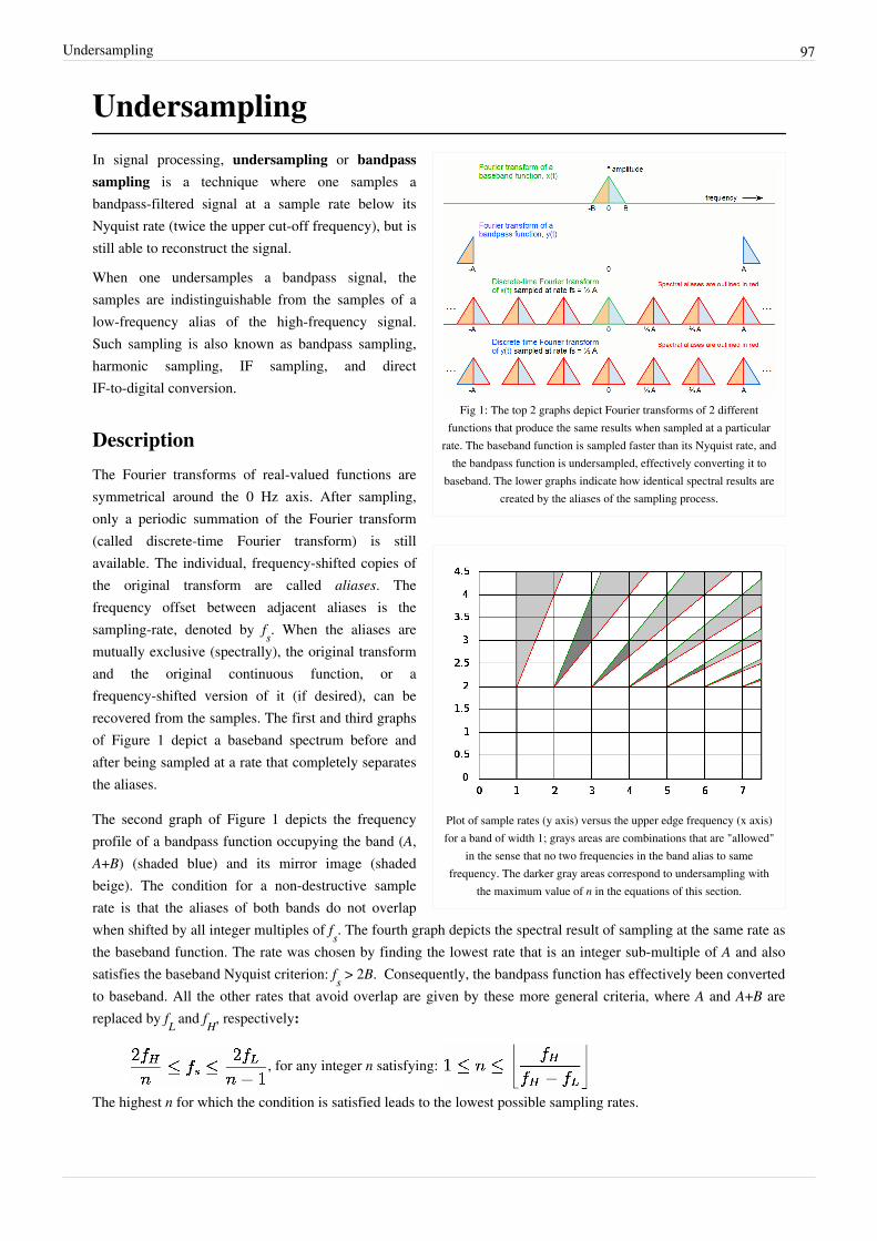
Undersampling 97
Undersampling
Fig 1: The top 2 graphs depict Fourier transforms of 2 differentfunctions that produce the same results when sampled at a particular
rate. The baseband function is sampled faster than its Nyquist rate, andthe bandpass function is undersampled, effectively converting it to
baseband. The lower graphs indicate how identical spectral results arecreated by the aliases of the sampling process.
Plot of sample rates (y axis) versus the upper edge frequency (x axis)for a band of width 1; grays areas are combinations that are "allowed"
in the sense that no two frequencies in the band alias to samefrequency. The darker gray areas correspond to undersampling with
the maximum value of n in the equations of this section.
In signal processing, undersampling or bandpasssampling is a technique where one samples abandpass-filtered signal at a sample rate below itsNyquist rate (twice the upper cut-off frequency), but isstill able to reconstruct the signal.
When one undersamples a bandpass signal, thesamples are indistinguishable from the samples of alow-frequency alias of the high-frequency signal.Such sampling is also known as bandpass sampling,harmonic sampling, IF sampling, and directIF-to-digital conversion.
Description
The Fourier transforms of real-valued functions aresymmetrical around the 0 Hz axis. After sampling,only a periodic summation of the Fourier transform(called discrete-time Fourier transform) is stillavailable. The individual, frequency-shifted copies ofthe original transform are called aliases. Thefrequency offset between adjacent aliases is thesampling-rate, denoted by fs. When the aliases aremutually exclusive (spectrally), the original transformand the original continuous function, or afrequency-shifted version of it (if desired), can berecovered from the samples. The first and third graphsof Figure 1 depict a baseband spectrum before andafter being sampled at a rate that completely separatesthe aliases.
The second graph of Figure 1 depicts the frequencyprofile of a bandpass function occupying the band (A,A+B) (shaded blue) and its mirror image (shadedbeige). The condition for a non-destructive samplerate is that the aliases of both bands do not overlapwhen shifted by all integer multiples of fs. The fourth graph depicts the spectral result of sampling at the same rate asthe baseband function. The rate was chosen by finding the lowest rate that is an integer sub-multiple of A and alsosatisfies the baseband Nyquist criterion: fs > 2B. Consequently, the bandpass function has effectively been convertedto baseband. All the other rates that avoid overlap are given by these more general criteria, where A and A+B arereplaced by fL and fH, respectively:
, for any integer n satisfying:
The highest n for which the condition is satisfied leads to the lowest possible sampling rates.
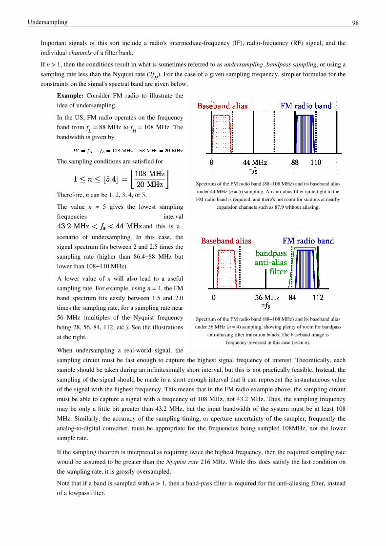
Undersampling 98
Important signals of this sort include a radio's intermediate-frequency (IF), radio-frequency (RF) signal, and theindividual channels of a filter bank.If n > 1, then the conditions result in what is sometimes referred to as undersampling, bandpass sampling, or using asampling rate less than the Nyquist rate (2fH). For the case of a given sampling frequency, simpler formulae for theconstraints on the signal's spectral band are given below.
Spectrum of the FM radio band (88–108 MHz) and its baseband aliasunder 44 MHz (n = 5) sampling. An anti-alias filter quite tight to theFM radio band is required, and there's not room for stations at nearby
expansion channels such as 87.9 without aliasing.
Spectrum of the FM radio band (88–108 MHz) and its baseband aliasunder 56 MHz (n = 4) sampling, showing plenty of room for bandpass
anti-aliasing filter transition bands. The baseband image isfrequency-reversed in this case (even n).
Example: Consider FM radio to illustrate theidea of undersampling.
In the US, FM radio operates on the frequencyband from fL = 88 MHz to fH = 108 MHz. Thebandwidth is given by
The sampling conditions are satisfied for
Therefore, n can be 1, 2, 3, 4, or 5.The value n = 5 gives the lowest samplingfrequencies interval
and this is ascenario of undersampling. In this case, thesignal spectrum fits between 2 and 2.5 times thesampling rate (higher than 86.4–88 MHz butlower than 108–110 MHz).
A lower value of n will also lead to a usefulsampling rate. For example, using n = 4, the FMband spectrum fits easily between 1.5 and 2.0times the sampling rate, for a sampling rate near56 MHz (multiples of the Nyquist frequencybeing 28, 56, 84, 112, etc.). See the illustrationsat the right.
When undersampling a real-world signal, thesampling circuit must be fast enough to capture the highest signal frequency of interest. Theoretically, eachsample should be taken during an infinitesimally short interval, but this is not practically feasible. Instead, thesampling of the signal should be made in a short enough interval that it can represent the instantaneous valueof the signal with the highest frequency. This means that in the FM radio example above, the sampling circuitmust be able to capture a signal with a frequency of 108 MHz, not 43.2 MHz. Thus, the sampling frequencymay be only a little bit greater than 43.2 MHz, but the input bandwidth of the system must be at least 108MHz. Similarly, the accuracy of the sampling timing, or aperture uncertainty of the sampler, frequently theanalog-to-digital converter, must be appropriate for the frequencies being sampled 108MHz, not the lowersample rate.
If the sampling theorem is interpreted as requiring twice the highest frequency, then the required sampling ratewould be assumed to be greater than the Nyquist rate 216 MHz. While this does satisfy the last condition onthe sampling rate, it is grossly oversampled.Note that if a band is sampled with n > 1, then a band-pass filter is required for the anti-aliasing filter, insteadof a lowpass filter.

Undersampling 99
As we have seen, the normal baseband condition for reversible sampling is that X(f) = 0 outside the interval:
and the reconstructive interpolation function, or lowpass filter impulse response, is To accommodate undersampling, the bandpass condition is that X(f) = 0 outside the union of open positive andnegative frequency bands
for some positive integer .
which includes the normal baseband condition as case n = 1 (except that where the intervals cometogether at 0 frequency, they can be closed).
The corresponding interpolation function is the bandpass filter given by this difference of lowpass impulseresponses:
.
On the other hand, reconstruction is not usually the goal with sampled IF or RF signals. Rather, the sample sequencecan be treated as ordinary samples of the signal frequency-shifted to near baseband, and digital demodulation canproceed on that basis, recognizing the spectrum mirroring when n is even.Further generalizations of undersampling for the case of signals with multiple bands are possible, and signals overmultidimensional domains (space or space-time) and have been worked out in detail by Igor Kluvánek.
References
Delta-sigma modulation"Sigma delta" redirects here. For the sorority, see Sigma Delta.Delta-sigma (ΔΣ; or sigma-delta, ΣΔ) modulation is a digital signal processing, or DSP method for encodinganalog signals into digital signals as found in an ADC. It is also used to transfer higher-resolution digital signals intolower-resolution digital signals as part of the process to convert digital signals into analog.In a conventional ADC, an analog signal is integrated, or sampled, with a sampling frequency and subsequentlyquantized in a multi-level quantizer into a digital signal. This process introduces quantization error noise. The firststep in a delta-sigma modulation is delta modulation. In delta modulation the change in the signal (its delta) isencoded, rather than the absolute value. The result is a stream of pulses, as opposed to a stream of numbers as is thecase with PCM. In delta-sigma modulation, the accuracy of the modulation is improved by passing the digital outputthrough a 1-bit DAC and adding (sigma) the resulting analog signal to the input signal, thereby reducing the errorintroduced by the delta-modulation.This technique has found increasing use in modern electronic components such as converters, frequencysynthesizers, switched-mode power supplies and motor controllers, primarily because of its cost efficiency andreduced circuit complexity.[1]
Both analog-to-digital converters (ADCs) and digital-to-analog converters (DACs) can employ delta-sigmamodulation. A delta-sigma ADC first encodes an analog signal using high-frequency delta-sigma modulation, andthen applies a digital filter to form a higher-resolution but lower sample-frequency digital output. On the other hand,a delta-sigma DAC encodes a high-resolution digital input signal into a lower-resolution but highersample-frequency signal that is mapped to voltages, and then smoothed with an analog filter. In both cases, thetemporary use of a lower-resolution signal simplifies circuit design and improves efficiency.
Delta-sigma modulation 100
The coarsely-quantized output of a delta-sigma modulator is occasionally used directly in signal processing or as arepresentation for signal storage. For example, the Super Audio CD (SACD) stores the output of a delta-sigmamodulator directly on a disk.
Motivation
Why convert an analog signal into a stream of pulses?In brief, because it is very easy to regenerate pulses at the receiver into the ideal form transmitted. The only part ofthe transmitted waveform required at the receiver is the time at which the pulse occurred. Given the timinginformation the transmitted waveform can be reconstructed electronically with great precision. In contrast, withoutconversion to a pulse stream but simply transmitting the analog signal directly, all noise in the system is added to theanalog signal, reducing its quality.Each pulse is made up of a step up followed after a short interval by a step down. It is possible, even in the presenceof electronic noise, to recover the timing of these steps and from that regenerate the transmitted pulse stream almostnoiselessly. Then the accuracy of the transmission process reduces to the accuracy with which the transmitted pulsestream represents the input waveform.
Why delta-sigma modulation?Delta-sigma modulation converts the analog voltage into a pulse frequency and is alternatively known as PulseDensity modulation or Pulse Frequency modulation. In general, frequency may vary smoothly in infinitesimal steps,as may voltage, and both may serve as an analog of an infinitesimally varying physical variable such as acousticpressure, light intensity, etc. The substitution of frequency for voltage is thus entirely natural and carries in its trainthe transmission advantages of a pulse stream. The different names for the modulation method are the result of pulsefrequency modulation by different electronic implementations, which all produce similar transmitted waveforms.
Why the delta-sigma analog to digital conversion?The ADC converts the mean of an analog voltage into the mean of an analog pulse frequency and counts the pulsesin a known interval so that the pulse count divided by the interval gives an accurate digital representation of themean analog voltage during the interval. This interval can be chosen to give any desired resolution or accuracy. Themethod is cheaply produced by modern methods; and it is widely used.
Analog to digital conversion
DescriptionThe ADC generates a pulse stream in which the frequency of pulses in the stream is proportional to the analogvoltage input, , so that the frequency, where k is a constant for the particular implementation.A counter sums the number of pulses that occur in a predetermined period, so that the sum, , is
.is chosen so that a digital display of the count, , is a display of with a predetermined scaling factor.
Because may take any designed value it may be made large enough to give any desired resolution or accuracy.Each pulse of the pulse stream has a known, constant amplitude and duration , and thus has a known integral
but variable separating interval.In a formal analysis an impulse such as integral is treated as the Dirac δ (delta) function and is specified by the
step produced on integration. Here we indicate that step as .
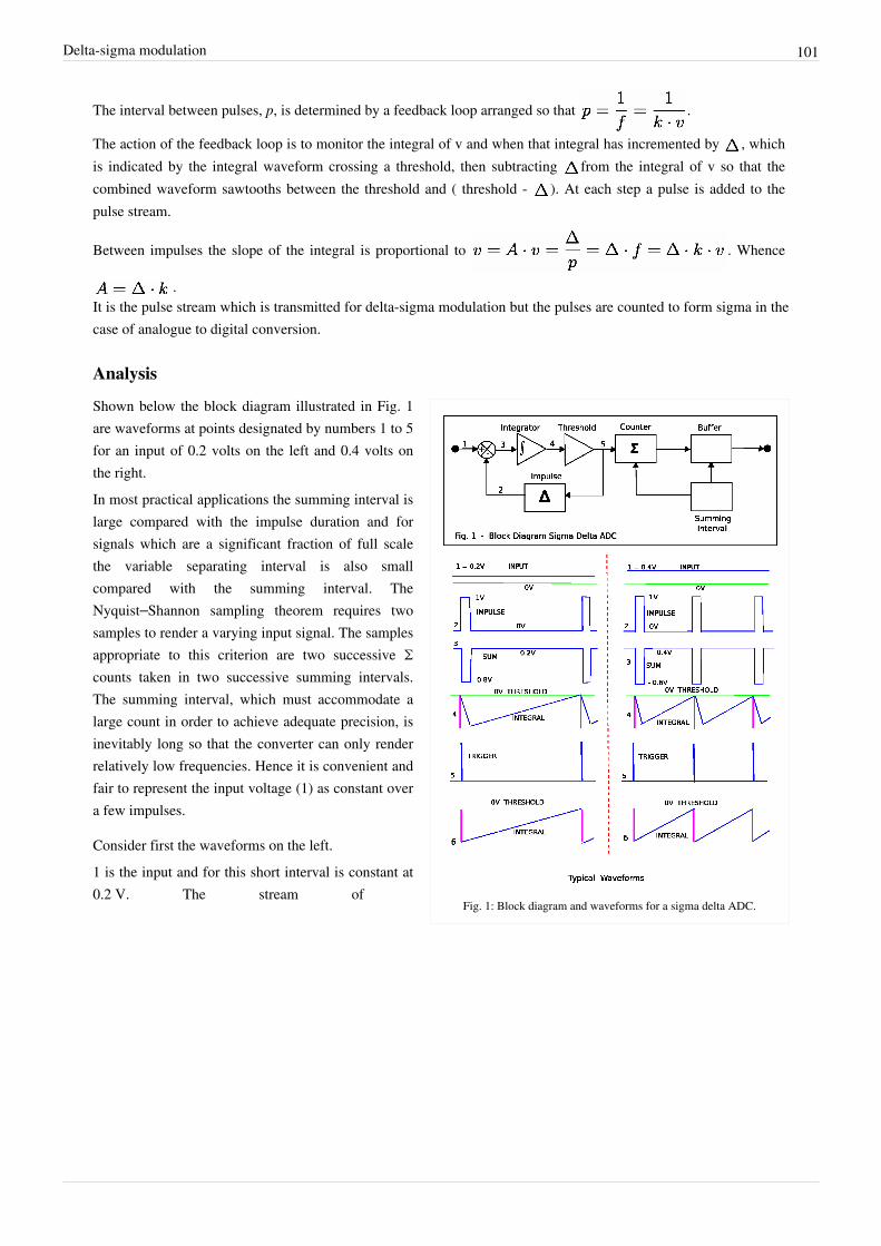
Delta-sigma modulation 101
The interval between pulses, p, is determined by a feedback loop arranged so that .
The action of the feedback loop is to monitor the integral of v and when that integral has incremented by , whichis indicated by the integral waveform crossing a threshold, then subtracting from the integral of v so that thecombined waveform sawtooths between the threshold and ( threshold - ). At each step a pulse is added to thepulse stream.
Between impulses the slope of the integral is proportional to . Whence
.It is the pulse stream which is transmitted for delta-sigma modulation but the pulses are counted to form sigma in thecase of analogue to digital conversion.
Analysis
Fig. 1: Block diagram and waveforms for a sigma delta ADC.
Shown below the block diagram illustrated in Fig. 1are waveforms at points designated by numbers 1 to 5for an input of 0.2 volts on the left and 0.4 volts onthe right.In most practical applications the summing interval islarge compared with the impulse duration and forsignals which are a significant fraction of full scalethe variable separating interval is also smallcompared with the summing interval. TheNyquist–Shannon sampling theorem requires twosamples to render a varying input signal. The samplesappropriate to this criterion are two successive Σcounts taken in two successive summing intervals.The summing interval, which must accommodate alarge count in order to achieve adequate precision, isinevitably long so that the converter can only renderrelatively low frequencies. Hence it is convenient andfair to represent the input voltage (1) as constant overa few impulses.
Consider first the waveforms on the left.1 is the input and for this short interval is constant at0.2 V. The stream of

Delta-sigma modulation 102
Fig. 1a: Effect of clocking impulses
delta impulses is shown at 2 and thedifference between 1 and 2 is shown at3. This difference is integrated toproduce the waveform 4. The thresholddetector generates a pulse 5 whichstarts as the waveform 4 crosses thethreshold and is sustained until thewaveform 4 falls below the threshold.Within the loop 5 triggers the impulsegenerator and external to the loopincrements the counter. The summinginterval is a prefixed time and at itsexpiry the count is strobed into thebuffer and the counter reset.It is necessary that the ratio betweenthe impulse interval and the summinginterval is equal to the maximum (full scale) count. It is then possible for the impulse duration and the summinginterval to be defined by the same clock with a suitable arrangement of logic and counters. This has the advantagethat neither interval has to be defined with absolute precision as only the ratio is important. Then to achieve overallaccuracy it is only necessary that the amplitude of the impulse be accurately defined.On the right the input is now 0.4 V and the sum during the impulse is −0.6 V as opposed to −0.8 V on the left. Thusthe negative slope during the impulse is lower on the right than on the left.Also the sum is 0.4 V on the right during the interval as opposed to 0.2 V on the left. Thus the positive slope outsidethe impulse is higher on the right than on the left.The resultant effect is that the integral (4) crosses the threshold more quickly on the right than on the left. A fullanalysis would show that in fact the interval between threshold crossings on the right is half that on the left. Thus thefrequency of impulses is doubled. Hence the count increments at twice the speed on the right to that on the left whichis consistent with the input voltage being doubled.Construction of the waveforms illustrated at (4) is aided by concepts associated with the Dirac delta function in thatall impulses of the same strength produce the same step when integrated, by definition. Then (4) is constructed usingan intermediate step (6) in which each integrated impulse is represented by a step of the assigned strength whichdecays to zero at the rate determined by the input voltage. The effect of the finite duration of the impulse isconstructed in (4) by drawing a line from the base of the impulse step at zero volts to intersect the decay line from(6) at the full duration of the impulse.As stated, Fig. 1 is a simplified block diagram of the delta-sigma ADC in which the various functional elements havebeen separated out for individual treatment and which tries to be independent of any particular implementation.Many particular implementations seek to define the impulse duration and the summing interval from the same clockas discussed above but in such a way that the start of the impulse is delayed until the next occurrence of theappropriate clock pulse boundary. The effect of this delay is illustrated in Fig. 1a for a sequence of impulses whichoccur at a nominal 2.5 clock intervals, firstly for impulses generated immediately the threshold is crossed aspreviously discussed and secondly for impulses delayed by the clock. The effect of the delay is firstly that the rampcontinues until the onset of the impulse, secondly that the impulse produces a fixed amplitude step so that theintegral retains the excess it acquired during the impulse delay and so the ramp restarts from a higher point and isnow on the same locus as the unclocked integral. The effect is that, for this example, the undelayed impulses willoccur at clock points 0, 2.5, 5, 7.5, 10, etc. and the clocked impulses will occur at 0, 3, 5, 8, 10, etc. The maximumerror that can occur due to clocking is marginally less than one count. Although the Sigma-Delta converter is
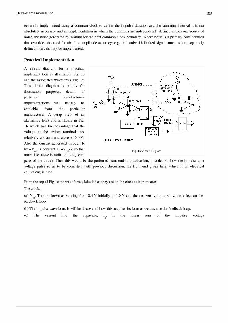
Delta-sigma modulation 103
generally implemented using a common clock to define the impulse duration and the summing interval it is notabsolutely necessary and an implementation in which the durations are independently defined avoids one source ofnoise, the noise generated by waiting for the next common clock boundary. Where noise is a primary considerationthat overrides the need for absolute amplitude accuracy; e.g., in bandwidth limited signal transmission, separatelydefined intervals may be implemented.
Practical Implementation
Fig. 1b: circuit diagram
A circuit diagram for a practicalimplementation is illustrated, Fig 1band the associated waveforms Fig. 1c.This circuit diagram is mainly forillustration purposes, details ofparticular manufacturersimplementations will usually beavailable from the particularmanufacturer. A scrap view of analternative front end is shown in Fig.1b which has the advantage that thevoltage at the switch terminals arerelatively constant and close to 0.0 V.Also the current generated through Rby −Vref is constant at −Vref/R so thatmuch less noise is radiated to adjacentparts of the circuit. Then this would be the preferred front end in practice but, in order to show the impulse as avoltage pulse so as to be consistent with previous discussion, the front end given here, which is an electricalequivalent, is used.
From the top of Fig 1c the waveforms, labelled as they are on the circuit diagram, are:-The clock.(a) Vin. This is shown as varying from 0.4 V initially to 1.0 V and then to zero volts to show the effect on thefeedback loop.
(b) The impulse waveform. It will be discovered how this acquires its form as we traverse the feedback loop.(c) The current into the capacitor, Ic, is the linear sum of the impulse voltage
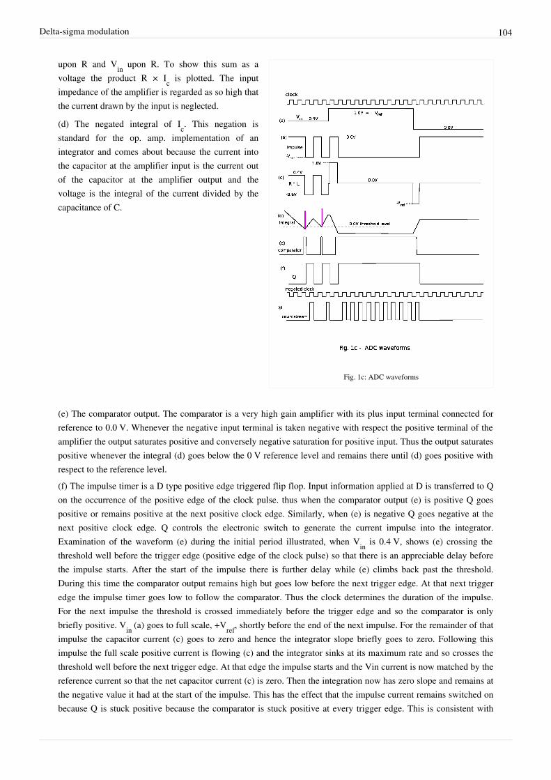
Delta-sigma modulation 104
Fig. 1c: ADC waveforms
upon R and Vin upon R. To show this sum as avoltage the product R × Ic is plotted. The inputimpedance of the amplifier is regarded as so high thatthe current drawn by the input is neglected.
(d) The negated integral of Ic. This negation isstandard for the op. amp. implementation of anintegrator and comes about because the current intothe capacitor at the amplifier input is the current outof the capacitor at the amplifier output and thevoltage is the integral of the current divided by thecapacitance of C.
(e) The comparator output. The comparator is a very high gain amplifier with its plus input terminal connected forreference to 0.0 V. Whenever the negative input terminal is taken negative with respect the positive terminal of theamplifier the output saturates positive and conversely negative saturation for positive input. Thus the output saturatespositive whenever the integral (d) goes below the 0 V reference level and remains there until (d) goes positive withrespect to the reference level.(f) The impulse timer is a D type positive edge triggered flip flop. Input information applied at D is transferred to Q on the occurrence of the positive edge of the clock pulse. thus when the comparator output (e) is positive Q goes positive or remains positive at the next positive clock edge. Similarly, when (e) is negative Q goes negative at the next positive clock edge. Q controls the electronic switch to generate the current impulse into the integrator. Examination of the waveform (e) during the initial period illustrated, when Vin is 0.4 V, shows (e) crossing the threshold well before the trigger edge (positive edge of the clock pulse) so that there is an appreciable delay before the impulse starts. After the start of the impulse there is further delay while (e) climbs back past the threshold. During this time the comparator output remains high but goes low before the next trigger edge. At that next trigger edge the impulse timer goes low to follow the comparator. Thus the clock determines the duration of the impulse. For the next impulse the threshold is crossed immediately before the trigger edge and so the comparator is only briefly positive. Vin (a) goes to full scale, +Vref, shortly before the end of the next impulse. For the remainder of that impulse the capacitor current (c) goes to zero and hence the integrator slope briefly goes to zero. Following this impulse the full scale positive current is flowing (c) and the integrator sinks at its maximum rate and so crosses the threshold well before the next trigger edge. At that edge the impulse starts and the Vin current is now matched by the reference current so that the net capacitor current (c) is zero. Then the integration now has zero slope and remains at the negative value it had at the start of the impulse. This has the effect that the impulse current remains switched on because Q is stuck positive because the comparator is stuck positive at every trigger edge. This is consistent with
Delta-sigma modulation 105
contiguous, butting impulses which is required at full scale input.Eventually Vin (a) goes to zero which means that the current sum (c) goes fully negative and the integral ramps up.It shortly thereafter crosses the threshold and this in turn is followed by Q, thus switching the impulse current off.The capacitor current (c) is now zero and so the integral slope is zero, remaining constant at the value it had acquiredat the end of the impulse.(g) The countstream is generated by gating the negated clock with Q to produce this waveform. Thereafter thesumming interval, sigma count and buffered count are produced using appropriate counters and registers. The Vinwaveform is approximated by passing the countstream (g) into a low pass filter, however it suffers from the defectdiscussed in the context of Fig. 1a. One possibility for reducing this error is to halve the feedback pulse length to halfa clock period and double its amplitude by halving the impulse defining resistor thus producing an impulse of thesame strength but one which never butts onto its adjacent impulses. Then there will be a threshold crossing for everyimpulse. In this arrangement a monostable flip flop triggered by the comparator at the threshold crossing will closelyfollow the threshold crossings and thus eliminate one source of error, both in the ADC and the sigma deltamodulator.
RemarksIn this section we have mainly dealt with the analogue to digital converter as a stand alone function which achievesastonishing accuracy with what is now a very simple and cheap architecture. Initially the Delta-Sigma configurationwas devised by INOSE et al. to solve problems in the accurate transmission of analog signals. In that application itwas the pulse stream that was transmitted and the original analog signal recovered with a low pass filter after thereceived pulses had been reformed. This low pass filter performed the summation function associated with Σ. Thehighly mathematical treatment of transmission errors was introduced by them and is appropriate when applied to thepulse stream but these errors are lost in the accumulation process associated with Σ to be replaced with the errorsassociated with the mean of means when discussing the ADC. For those uncomfortable with this assertion considerthis.It is well known that by Fourier analysis techniques the incoming waveform can be represented over the summinginterval by the sum of a constant plus a fundamental and harmonics each of which has an exact integer number ofcycles over the sampling period. It is also well known that the integral of a sine wave or cosine wave over one ormore full cycles is zero. Then the integral of the incoming waveform over the summing interval reduces to theintegral of the constant and when that integral is divided by the summing interval it becomes the mean over thatinterval. The interval between pulses is proportional to the inverse of the mean of the input voltage during thatinterval and thus over that interval, ts, is a sample of the mean of the input voltage proportional to V/ts. Thus theaverage of the input voltage over the summing period is VΣ/N and is the mean of means and so subject to littlevariance.Unfortunately the analysis for the transmitted pulse stream has, in many cases, been carried over, uncritically, to theADC.It was indicated in section 2.2 Analysis that the effect of constraining a pulse to only occur on clock boundaries is tointroduce noise, that generated by waiting for the next clock boundary. This will have its most deleterious effect onthe high frequency components of a complex signal. Whilst the case has been made for clocking in the ADCenvironment, where it removes one source of error, namely the ratio between the impulse duration and the summinginterval, it is deeply unclear what useful purpose clocking serves in a single channel transmission environment sinceit is a source of both noise and complexity but it is conceivable that it would be useful in a TDM (time divisionmultiplex) environment.A very accurate transmission system with constant sampling rate may be formed using the full arrangement shownhere by transmitting the samples from the buffer protected with redundancy error correction. In this case there willbe a trade off between bandwidth and N, the size of the buffer. The signal recovery system will require redundancy
Delta-sigma modulation 106
error checking, digital to analog conversion,and sample and hold circuitry. A possible further enhancement is toinclude some form of slope regeneration.This amounts to PCM (pulse code modulation) with digitization performedby a sigma-delta ADC.The above description shows why the impulse is called delta. The integral of an impulse is a step. A one bit DACmay be expected to produce a step and so must be a conflation of an impulse and an integration. The analysis whichtreats the impulse as the output of a 1-bit DAC hides the structure behind the name (sigma delta) and causeconfusion and difficulty interpreting the name as an indication of function. This analysis is very widespread but isdeprecated.A modern alternative method for generating voltage to frequency conversion is discussed in synchronous voltage tofrequency converter (SVFC) which may be followed by a counter to produce a digital representation in a similarmanner to that described above.[2]
Digital to analog conversion
DiscussionDelta-sigma modulators are often used in digital to analog converters (DACs). In general, a DAC converts a digitalnumber representing some analog value into that analog value. For example, the analog voltage level into a speakermay be represented as a 20 bit digital number, and the DAC converts that number into the desired voltage. Toactually drive a load (like a speaker) a DAC is usually connected to or integrated with an electronic amplifier.This can be done using a delta-sigma modulator in a Class D Amplifier. In this case, a multi-bit digital number isinput to the delta-sigma modulator, which converts it into a faster sequence of 0's and 1's. These 0's and 1's are thenconverted into analog voltages. The conversion, usually with MOSFET drivers, is very efficient in terms of powerbecause the drivers are usually either fully on or fully off, and in these states have low power loss.The resulting two-level signal is now like the desired signal, but with higher frequency components to change thesignal so that it only has two levels. These added frequency components arise from the quantization error of thedelta-sigma modulator, but can be filtered away by a simple low-pass filter. The result is a reproduction of theoriginal, desired analog signal from the digital values.The circuit itself is relatively inexpensive. The digital circuit is small, and the MOSFETs used for the poweramplification are simple. This is in contrast to a multi-bit DAC which can have very stringent design conditions toprecisely represent digital values with a large number of bits.The use of a delta-sigma modulator in the digital to analog conversion has enabled a cost-effective, low power, andhigh performance solution.

Delta-sigma modulation 107
Relationship to Δ-modulation
Fig. 2: Derivation of ΔΣ- from Δ-modulation
ΔΣ modulation (SDM) is inspired by Δmodulation (DM), as shown in Fig. 2.If quantization were homogeneous(e.g., if it were linear), the followingwould be a sufficient derivation of theequivalence of DM and SDM:
1.1. Start with a block diagram of aΔ-modulator/demodulator.
2. The linearity property of integration( ) makes itpossible to move the integrator,which reconstructs the analog signalin the demodulator section, in frontof the Δ-modulator.
3.3. Again, the linearity property of theintegration allows the twointegrators to be combined and aΔΣ-modulator/demodulator blockdiagram is obtained.
However, the quantizer is not homogeneous, and so this explanation is flawed. It's true that ΔΣ is inspired byΔ-modulation, but the two are distinct in operation. From the first block diagram in Fig. 2, the integrator in thefeedback path can be removed if the feedback is taken directly from the input of the low-pass filter. Hence, for deltamodulation of input signal , the low-pass filter sees the signal
However, sigma-delta modulation of the same input signal places at the low-pass filter
In other words, SDM and DM swap the position of the integrator and quantizer. The net effect is a simplerimplementation that has the added benefit of shaping the quantization noise away from signals of interest (i.e.,signals of interest are low-pass filtered while quantization noise is high-pass filtered). This effect becomes moredramatic with increased oversampling, which allows for quantization noise to be somewhat programmable. On theother hand, Δ-modulation shapes both noise and signal equally.Additionally, the quantizer (e.g., comparator) used in DM has a small output representing a small step up and downthe quantized approximation of the input while the quantizer used in SDM must take values outside of the range ofthe input signal, as shown in Fig. 3.
Fig. 3: An example of SDM of 100 samples of one period a sine wave. 1-bit samples (e.g., comparator output) overlaid with sine wavewhere logic high (e.g., ) represented by blue and logic low (e.g., ) represented by white.
In general, ΔΣ has some advantages versus Δ modulation:

Delta-sigma modulation 108
•• The whole structure is simpler:•• Only one integrator is needed•• The demodulator can be a simple linear filter (e.g., RC or LC filter) to reconstruct the signal•• The quantizer (e.g., comparator) can have full-scale outputs
•• The quantized value is the integral of the difference signal, which makes it less sensitive to the rate of change ofthe signal.
PrincipleThe principle of the ΔΣ architecture is explained at length in section 2. Initially, when a sequence starts, the circuitwill have an arbitrary state which is dependant on the integral of all previous history. In mathematical terms thiscorresponds to the arbitrary integration constant of the indefinite integral. This follows from the fact that at the heartof the method there is an integrator which can have any arbitrary state dependant on previous input, see Fig. 1c (d).From the occurrence of the first pulse onward the frequency of the pulse stream is proportional to the input voltageto be transformed. A demonstration applet is available online to simulate the whole architecture.[3]
VariationsThere are many kinds of ADC that use this delta-sigma structure. The above analysis focuses on the simplest1st-order, 2-level, uniform-decimation sigma-delta ADC. Many ADCs use a second-order 5-level sinc3 sigma-deltastructure.
2nd order and higher order modulator
Fig. 4: Block diagram of a 2nd order ΔΣ modulator
The number of integrators, andconsequently, the numbers of feedbackloops, indicates the order of aΔΣ-modulator; a 2nd order ΔΣmodulator is shown in Fig. 4. Firstorder modulators are unconditionallystable, but stability analysis must beperformed for higher order modulators.
3-level and higher quantizerThe modulator can also be classified by the number of bits it has in output, which strictly depends on the output ofthe quantizer. The quantizer can be realized with a N-level comparator, thus the modulator has log2N-bit output. Asimple comparator has 2 levels and so is 1 bit quantizer; a 3-level quantizer is called a "1.5" bit quantizer; a 4-levelquantizer is a 2 bit quantizer; a 5-level quantizer is called a "2.5 bit" quantizer.[4]
Decimation structuresThe conceptually simplest decimation structure is a counter that is reset to zero at the beginning of each integrationperiod, then read out at the end of the integration period.The multi-stage noise shaping (MASH) structure has a noise shaping property, and is commonly used in digitalaudio and fractional-N frequency synthesizers. It comprises two or more cascaded overflowing accumulators, each ofwhich is equivalent to a first-order sigma delta modulator. The carry outputs are combined through summations anddelays to produce a binary output, the width of which depends on the number of stages (order) of the MASH.Besides its noise shaping function, it has two more attractive properties:
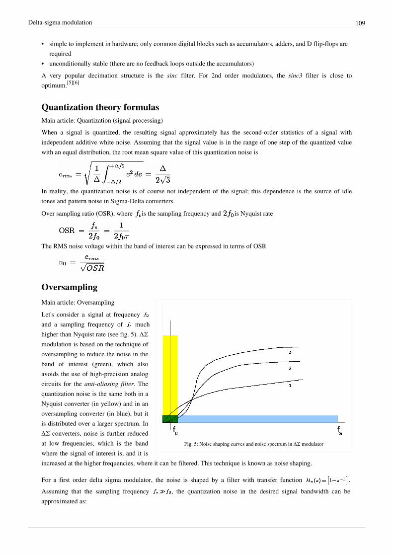
Delta-sigma modulation 109
• simple to implement in hardware; only common digital blocks such as accumulators, adders, and D flip-flops arerequired
•• unconditionally stable (there are no feedback loops outside the accumulators)A very popular decimation structure is the sinc filter. For 2nd order modulators, the sinc3 filter is close tooptimum.[5][6]
Quantization theory formulasMain article: Quantization (signal processing)When a signal is quantized, the resulting signal approximately has the second-order statistics of a signal withindependent additive white noise. Assuming that the signal value is in the range of one step of the quantized valuewith an equal distribution, the root mean square value of this quantization noise is
In reality, the quantization noise is of course not independent of the signal; this dependence is the source of idletones and pattern noise in Sigma-Delta converters.
Over sampling ratio (OSR), where is the sampling frequency and is Nyquist rate
The RMS noise voltage within the band of interest can be expressed in terms of OSR
Oversampling
Fig. 5: Noise shaping curves and noise spectrum in ΔΣ modulator
Main article: OversamplingLet's consider a signal at frequency and a sampling frequency of muchhigher than Nyquist rate (see fig. 5). ΔΣmodulation is based on the technique ofoversampling to reduce the noise in theband of interest (green), which alsoavoids the use of high-precision analogcircuits for the anti-aliasing filter. Thequantization noise is the same both in aNyquist converter (in yellow) and in anoversampling converter (in blue), but itis distributed over a larger spectrum. InΔΣ-converters, noise is further reducedat low frequencies, which is the bandwhere the signal of interest is, and it isincreased at the higher frequencies, where it can be filtered. This technique is known as noise shaping.
For a first order delta sigma modulator, the noise is shaped by a filter with transfer function .Assuming that the sampling frequency , the quantization noise in the desired signal bandwidth can beapproximated as:

Delta-sigma modulation 110
.
Similarly for a second order delta sigma modulator, the noise is shaped by a filter with transfer function. The in-band quantization noise can be approximated as:
.
In general, for a -order ΔΣ-modulator, the variance of the in-band quantization noise:
.
When the sampling frequency is doubled, the signal to quantization noise is improved by for a -order ΔΣ-modulator. The higher the oversampling ratio, the higher the signal-to-noise ratio and the higher theresolution in bits.Another key aspect given by oversampling is the speed/resolution tradeoff. In fact, the decimation filter put after themodulator not only filters the whole sampled signal in the band of interest (cutting the noise at higher frequencies),but also reduces the frequency of the signal increasing its resolution. This is obtained by a sort of averaging of thehigher data rate bitstream.
Example of decimationLet's have, for instance, an 8:1 decimation filter and a 1-bit bitstream; if we have an input stream like 10010110,counting the number of ones, we get 4. Then the decimation result is 4/8 = 0.5. We can then represent it with a 3-bitsnumber 100 (binary), which means half of the largest possible number. In other words,•• the sample frequency is reduced by a factor of eight•• the serial (1-bit) input bus becomes a parallel (3-bits) output bus.
NamingThe technique was first presented in the early 1960s by professor Haruhiko Yasuda while he was a student atWaseda University, Tokyo, Japan.Wikipedia:Citation needed The name Delta-Sigma comes directly from thepresence of a Delta modulator and an integrator, as firstly introduced by Inose et al. in their patent application.[7]
That is, the name comes from integrating or "summing" differences, which are operations usually associated withGreek letters Sigma and Delta respectively. Both names Sigma-Delta and Delta-Sigma are frequently used.
References[1] http:/ / www. numerix-dsp. com/ appsnotes/ APR8-sigma-delta. pdf[2] Voltage-to-Frequency Converters (http:/ / www. analog. com/ static/ imported-files/ tutorials/ MT-028. pdf) by Walt Kester and James Bryant
2009. Analog Devices.[3] Analog Devices : Virtual Design Center : Interactive Design Tools : Sigma-Delta ADC Tutorial (http:/ / designtools. analog. com/ dt/
sdtutorial/ sdtutorial. html)[4] Sigma-delta class-D amplifier and control method for a sigma-delta class-D amplifier (http:/ / www. faqs. org/ patents/ app/ 20090072897) by
Jwin-Yen Guo and Teng-Hung Chang[5] A Novel Architecture for DAQ in Multi-channel, Large Volume, Long Drift Liquid Argon TPC (http:/ / www. slac. stanford. edu/ econf/
C0604032/ papers/ 0232. PDF) by S. Centro, G. Meng, F. Pietropaola, S. Ventura 2006[6] A Low Power Sinc3 Filter for ΣΔ Modulators (http:/ / ieeexplore. ieee. org/ xpl/ freeabs_all. jsp?arnumber=4253561) by A. Lombardi, E.
Bonizzoni, P. Malcovati, F. Maloberti 2007[7][7] H. Inose, Y. Yasuda, J. Murakami, "A Telemetering System by Code Manipulation -- ΔΣ Modulation", IRE Trans on Space Electronics and
Telemetry, Sep. 1962, pp. 204-209.
• Walt Kester (October 2008). "ADC Architectures III: Sigma-Delta ADC Basics" (http:/ / www. analog. com/static/ imported-files/ tutorials/ MT-022. pdf) (PDF). Analog Devices. Retrieved 2010-11-02.
Delta-sigma modulation 111
• R. Jacob Baker (2009). CMOS Mixed-Signal Circuit Design (http:/ / CMOSedu. com/ ) (2nd ed.). Wiley-IEEE.ISBN 978-0-470-29026-2.
• R. Schreier, G. Temes (2005). Understanding Delta-Sigma Data Converters. ISBN 0-471-46585-2.• S. Norsworthy, R. Schreier, G. Temes (1997). Delta-Sigma Data Converters. ISBN 0-7803-1045-4.• J. Candy, G. Temes (1992). Oversampling Delta-sigma Data Converters. ISBN 0-87942-285-8.
External links• 1-bit A/D and D/A Converters (http:/ / www. cs. tut. fi/ sgn/ arg/ rosti/ 1-bit/ )• Sigma-delta techniques extend DAC resolution (http:/ / www. embedded. com/ design/ configurable-systems/
4006431/ Sigma-delta-techniques-extend-DAC-resolution) article by Tim Wescott 2004-06-23• Tutorial on Designing Delta-Sigma Modulators: Part I (http:/ / www. commsdesign. com/ design_corner/
showArticle. jhtml?articleID=18402743) and Part II (http:/ / www. commsdesign. com/ design_corner/showArticle. jhtml?articleID=18402763) by Mingliang (Michael) Liu
• Gabor Temes' Publications (http:/ / eecs. oregonstate. edu/ research/ members/ temes/ pubs. html)• Simple Sigma Delta Modulator example (http:/ / electronjunkie. wordpress. com/ tag/ sigma-delta-modulation/ )
Contains Block-diagrams, code, and simple explanations• Example Simulink model & scripts for continuous-time sigma-delta ADC (http:/ / www. circuitdesign. info/ blog/
2008/ 09/ example-simulink-model-scripts/ ) Contains example matlab code and Simulink model• Bruce Wooley's Delta-Sigma Converter Projects (http:/ / www-cis. stanford. edu/ icl/ wooley-grp/ projects. html)• An Introduction to Delta Sigma Converters (http:/ / www. beis. de/ Elektronik/ DeltaSigma/ DeltaSigma. html)
(which covers both ADC's and DAC's sigma-delta)• Demystifying Sigma-Delta ADCs (http:/ / www. maxim-ic. com/ appnotes. cfm/ an_pk/ 1870/ CMP/ WP-10).
This in-depth article covers the theory behind a Delta-Sigma analog-to-digital converter.• Motorola digital signal processors: Principles of sigma-delta modulation for analog-to-digital converters (http:/ /
digitalsignallabs. com/ SigmaDelta. pdf)• One-Bit Delta Sigma D/A Conversion Part I: Theory (http:/ / www. digitalsignallabs. com/ presentation. pdf)
article by Randy Yates presented at the 2004 comp.dsp conference• MASH (Multi-stAge noise SHaping) structure (http:/ / www. aholme. co. uk/ Frac2/ Mash. htm) with both theory
and a block-level implementation of a MASH• Continuous time sigma-delta ADC noise shaping filter circuit architectures (http:/ / www. circuitdesign. info/
blog/ 2008/ 11/ continuous-time-sigma-delta-adc-noise-shaping-filter-circuit-architectures-2/ ) discussesarchitectural trade-offs for continuous-time sigma-delta noise-shaping filters
• Some intuitive motivation for why a Delta Sigma modulator works (http:/ / www. cardinalpeak. com/ blog/?p=392/ )

Jitter 112
JitterFor other meanings of this word, see Jitter (disambiguation).Jitter is the undesired deviation from true periodicity of an assumed periodic signal in electronics andtelecommunications, often in relation to a reference clock source. Jitter may be observed in characteristics such asthe frequency of successive pulses, the signal amplitude, or phase of periodic signals. Jitter is a significant, andusually undesired, factor in the design of almost all communications links (e.g., USB, PCI-e, SATA, OC-48). Inclock recovery applications it is called timing jitter.[1]
Jitter can be quantified in the same terms as all time-varying signals, e.g., RMS, or peak-to-peak displacement. Alsolike other time-varying signals, jitter can be expressed in terms of spectral density (frequency content).Jitter period is the interval between two times of maximum effect (or minimum effect) of a signal characteristic thatvaries regularly with time. Jitter frequency, the more commonly quoted figure, is its inverse. ITU-T G.810 classifiesjitter frequencies below 10 Hz as wander and frequencies at or above 10 Hz as jitter.Jitter may be caused by electromagnetic interference (EMI) and crosstalk with carriers of other signals. Jitter cancause a display monitor to flicker, affect the performance of processors in personal computers, introduce clicks orother undesired effects in audio signals, and loss of transmitted data between network devices. The amount oftolerable jitter depends on the affected application.
Sampling jitterIn analog to digital and digital to analog conversion of signals, the sampling is normally assumed to be periodic witha fixed period—the time between every two samples is the same. If there is jitter present on the clock signal to theanalog-to-digital converter or a digital-to-analog converter, the time between samples varies and instantaneous signalerror arises. The error is proportional to the slew rate of the desired signal and the absolute value of the clock error.Various effects such as noise (random jitter), or spectral components (periodic jitter)Wikipedia:Citing sources cancome about depending on the pattern of the jitter in relation to the signal. In some conditions, less than a nanosecondof jitter can reduce the effective bit resolution of a converter with a Nyquist frequency of 22 kHz to 14bits.Wikipedia:Citation neededThis is a consideration in high-frequency signal conversion, or where the clock signal is especially prone tointerference.
Packet jitter in computer networksMain article: Packet delay variationIn the context of computer networks, jitter is the variation in latency as measured in the variability over time of thepacket latency across a network. A network with constant latency has no variation (or jitter). Packet jitter isexpressed as an average of the deviation from the network mean latency. However, for this use, the term isimprecise. The standards-based term is "packet delay variation" (PDV).[2] PDV is an important quality of servicefactor in assessment of network performance.
Compact disc seek jitterIn the context of digital audio extraction from Compact Discs, seek jitter causes extracted audio samples to be doubled-up or skipped entirely if the Compact Disc drive re-seeks. The problem occurs because the Red Book does not require block-accurate addressing during seeking. As a result, the extraction process may restart a few samples early or late, resulting in doubled or omitted samples. These glitches often sound like tiny repeating clicks during playback. A successful approach to correction in software involves performing overlapping reads and fitting the data
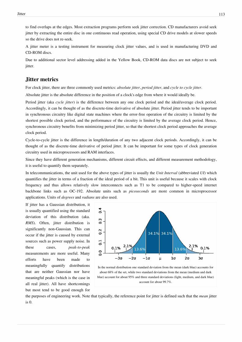
Jitter 113
to find overlaps at the edges. Most extraction programs perform seek jitter correction. CD manufacturers avoid seekjitter by extracting the entire disc in one continuous read operation, using special CD drive models at slower speedsso the drive does not re-seek.A jitter meter is a testing instrument for measuring clock jitter values, and is used in manufacturing DVD andCD-ROM discs.Due to additional sector level addressing added in the Yellow Book, CD-ROM data discs are not subject to seekjitter.
Jitter metricsFor clock jitter, there are three commonly used metrics: absolute jitter, period jitter, and cycle to cycle jitter.Absolute jitter is the absolute difference in the position of a clock's edge from where it would ideally be.Period jitter (aka cycle jitter) is the difference between any one clock period and the ideal/average clock period.Accordingly, it can be thought of as the discrete-time derivative of absolute jitter. Period jitter tends to be importantin synchronous circuitry like digital state machines where the error-free operation of the circuitry is limited by theshortest possible clock period, and the performance of the circuitry is limited by the average clock period. Hence,synchronous circuitry benefits from minimizing period jitter, so that the shortest clock period approaches the averageclock period.Cycle-to-cycle jitter is the difference in length/duration of any two adjacent clock periods. Accordingly, it can bethought of as the discrete-time derivative of period jitter. It can be important for some types of clock generationcircuitry used in microprocessors and RAM interfaces.Since they have different generation mechanisms, different circuit effects, and different measurement methodology,it is useful to quantify them separately.In telecommunications, the unit used for the above types of jitter is usually the Unit Interval (abbreviated UI) whichquantifies the jitter in terms of a fraction of the ideal period of a bit. This unit is useful because it scales with clockfrequency and thus allows relatively slow interconnects such as T1 to be compared to higher-speed internetbackbone links such as OC-192. Absolute units such as picoseconds are more common in microprocessorapplications. Units of degrees and radians are also used.
In the normal distribution one standard deviation from the mean (dark blue) accounts forabout 68% of the set, while two standard deviations from the mean (medium and dark
blue) account for about 95% and three standard deviations (light, medium, and dark blue)account for about 99.7%.
If jitter has a Gaussian distribution, itis usually quantified using the standarddeviation of this distribution (aka.RMS). Often, jitter distribution issignificantly non-Gaussian. This canoccur if the jitter is caused by externalsources such as power supply noise. Inthese cases, peak-to-peakmeasurements are more useful. Manyefforts have been made tomeaningfully quantify distributionsthat are neither Gaussian nor havemeaningful peaks (which is the case inall real jitter). All have shortcomingsbut most tend to be good enough forthe purposes of engineering work. Note that typically, the reference point for jitter is defined such that the mean jitteris 0.
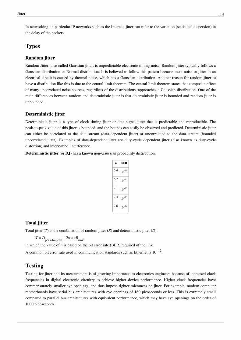
Jitter 114
In networking, in particular IP networks such as the Internet, jitter can refer to the variation (statistical dispersion) inthe delay of the packets.
Types
Random jitterRandom Jitter, also called Gaussian jitter, is unpredictable electronic timing noise. Random jitter typically follows aGaussian distribution or Normal distribution. It is believed to follow this pattern because most noise or jitter in anelectrical circuit is caused by thermal noise, which has a Gaussian distribution. Another reason for random jitter tohave a distribution like this is due to the central limit theorem. The central limit theorem states that composite effectof many uncorrelated noise sources, regardless of the distributions, approaches a Gaussian distribution. One of themain differences between random and deterministic jitter is that deterministic jitter is bounded and random jitter isunbounded.
Deterministic jitterDeterministic jitter is a type of clock timing jitter or data signal jitter that is predictable and reproducible. Thepeak-to-peak value of this jitter is bounded, and the bounds can easily be observed and predicted. Deterministic jittercan either be correlated to the data stream (data-dependent jitter) or uncorrelated to the data stream (boundeduncorrelated jitter). Examples of data-dependent jitter are duty-cycle dependent jitter (also known as duty-cycledistortion) and intersymbol interference.Deterministic jitter (or DJ) has a known non-Gaussian probability distribution.
n BER
6.4 10−10
6.7 10−11
7 10−12
7.3 10−13
7.6 10−14
Total jitterTotal jitter (T) is the combination of random jitter (R) and deterministic jitter (D):
T = Dpeak-to-peak + 2× n×Rrms,in which the value of n is based on the bit error rate (BER) required of the link.A common bit error rate used in communication standards such as Ethernet is 10−12.
TestingTesting for jitter and its measurement is of growing importance to electronics engineers because of increased clockfrequencies in digital electronic circuitry to achieve higher device performance. Higher clock frequencies havecommensurately smaller eye openings, and thus impose tighter tolerances on jitter. For example, modern computermotherboards have serial bus architectures with eye openings of 160 picoseconds or less. This is extremely smallcompared to parallel bus architectures with equivalent performance, which may have eye openings on the order of1000 picoseconds.
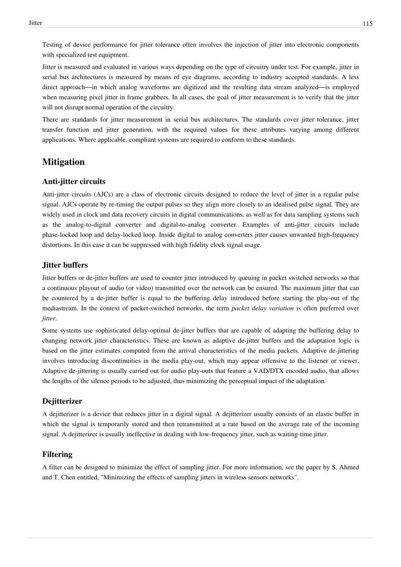
Jitter 115
Testing of device performance for jitter tolerance often involves the injection of jitter into electronic componentswith specialized test equipment.Jitter is measured and evaluated in various ways depending on the type of circuitry under test. For example, jitter inserial bus architectures is measured by means of eye diagrams, according to industry accepted standards. A lessdirect approach—in which analog waveforms are digitized and the resulting data stream analyzed—is employedwhen measuring pixel jitter in frame grabbers. In all cases, the goal of jitter measurement is to verify that the jitterwill not disrupt normal operation of the circuitry.There are standards for jitter measurement in serial bus architectures. The standards cover jitter tolerance, jittertransfer function and jitter generation, with the required values for these attributes varying among differentapplications. Where applicable, compliant systems are required to conform to these standards.
Mitigation
Anti-jitter circuitsAnti-jitter circuits (AJCs) are a class of electronic circuits designed to reduce the level of jitter in a regular pulsesignal. AJCs operate by re-timing the output pulses so they align more closely to an idealised pulse signal. They arewidely used in clock and data recovery circuits in digital communications, as well as for data sampling systems suchas the analog-to-digital converter and digital-to-analog converter. Examples of anti-jitter circuits includephase-locked loop and delay-locked loop. Inside digital to analog converters jitter causes unwanted high-frequencydistortions. In this case it can be suppressed with high fidelity clock signal usage.
Jitter buffersJitter buffers or de-jitter buffers are used to counter jitter introduced by queuing in packet switched networks so thata continuous playout of audio (or video) transmitted over the network can be ensured. The maximum jitter that canbe countered by a de-jitter buffer is equal to the buffering delay introduced before starting the play-out of themediastream. In the context of packet-switched networks, the term packet delay variation is often preferred overjitter.Some systems use sophisticated delay-optimal de-jitter buffers that are capable of adapting the buffering delay tochanging network jitter characteristics. These are known as adaptive de-jitter buffers and the adaptation logic isbased on the jitter estimates computed from the arrival characteristics of the media packets. Adaptive de-jitteringinvolves introducing discontinuities in the media play-out, which may appear offensive to the listener or viewer.Adaptive de-jittering is usually carried out for audio play-outs that feature a VAD/DTX encoded audio, that allowsthe lengths of the silence periods to be adjusted, thus minimizing the perceptual impact of the adaptation.
DejitterizerA dejitterizer is a device that reduces jitter in a digital signal. A dejitterizer usually consists of an elastic buffer inwhich the signal is temporarily stored and then retransmitted at a rate based on the average rate of the incomingsignal. A dejitterizer is usually ineffective in dealing with low-frequency jitter, such as waiting-time jitter.
FilteringA filter can be designed to minimize the effect of sampling jitter. For more information, see the paper by S. Ahmedand T. Chen entitled, "Minimizing the effects of sampling jitters in wireless sensors networks".

Jitter 116
Video and image jitterVideo or image jitter occurs when the horizontal lines of video image frames are randomly displaced due to thecorruption of synchronization signals or electromagnetic interference during video transmission. Model baseddejittering study has been carried out under the framework of digital image/video restoration.
Notes[1][1] Wolaver, 1991, p.211[2] RFC 3393, IP Packet Delay Variation Metric for IP Performance Metrics (IPPM), IETF (2002)
References• This article incorporates public domain material from the General Services Administration document "Federal
Standard 1037C" (http:/ / www. its. bldrdoc. gov/ fs-1037/ fs-1037c. htm) (in support of MIL-STD-188).• Trischitta, Patrick R. and Varma, Eve L. (1989). Jitter in Digital Transmission Systems. Artech. ISBN
0-89006-248-X.• Wolaver, Dan H. (1991). Phase-Locked Loop Circuit Design. Prentice Hall. ISBN 0-13-662743-9. pages
211–237.
Further reading• Levin, Igor. Terms and concepts involved with digital clocking related to Jitter issues in professional quality
digital audio (http:/ / www. antelopeaudio. com/ blog/ word-clock-sync-jitter/ )• Li, Mike P. Jitter and Signal Integrity Verification for Synchronous and Asynchronous I/Os at Multiple to 10
GHz/Gbps (http:/ / www. altera. com/ literature/ cp/ cp-01049-jitter-si-verification. pdf). Presented atInternational Test Conference 2008.
• Li, Mike P. A New Jitter Classification Method Based on Statistical, Physical, and Spectroscopic Mechanisms(http:/ / www. altera. com/ literature/ cp/ cp-01052-jitter-classification. pdf). Presented at DesignCon 2009.
• Liu, Hui, Hong Shi, Xiaohong Jiang, and Zhe Li. Pre-Driver PDN SSN, OPD, Data Encoding, and Their Impacton SSJ (http:/ / www. altera. com/ literature/ cp/ cp-01055-impact-ssj. pdf). Presented at Electronics Componentsand Technology Conference 2009.
• Miki, Ohtani, and Kowalski Jitter Requirements (https:/ / mentor. ieee. org/ 802. 11/ dcn/ 04/11-04-1458-00-000n-jitter-requirements. ppt) (Causes, solutions and recommended values for digital audio)
• Zamek, Iliya. SOC-System Jitter Resonance and Its Impact on Common Approach to the PDN Impedance (http:/ /www. altera. com/ literature/ cp/ cp-01048-jitter-resonance. pdf). Presented at International Test Conference2008.
External links• Jitter in VoIP - Causes, solutions and recommended values (http:/ / www. en. voipforo. com/ QoS/ QoS_Jitter.
php)• Jitter Buffer (http:/ / searchenterprisevoice. techtarget. com/ sDefinition/ 0,,sid66_gci906844,00. html)• Definition of Jitter in a QoS Testing Methodology (ftp:/ / ftp. iol. unh. edu/ pub/ mplsServices/ other/
QoS_Testing_Methodology. pdf)• An Introduction to Jitter in Communications Systems (http:/ / www. maxim-ic. com/ appnotes. cfm/ an_pk/ 1916/
CMP/ WP-34)• Jitter Specifications Made Easy (http:/ / www. maxim-ic. com/ appnotes. cfm/ an_pk/ 377/ CMP/ WP-35) A
Heuristic Discussion of Fibre Channel and Gigabit Ethernet Methods
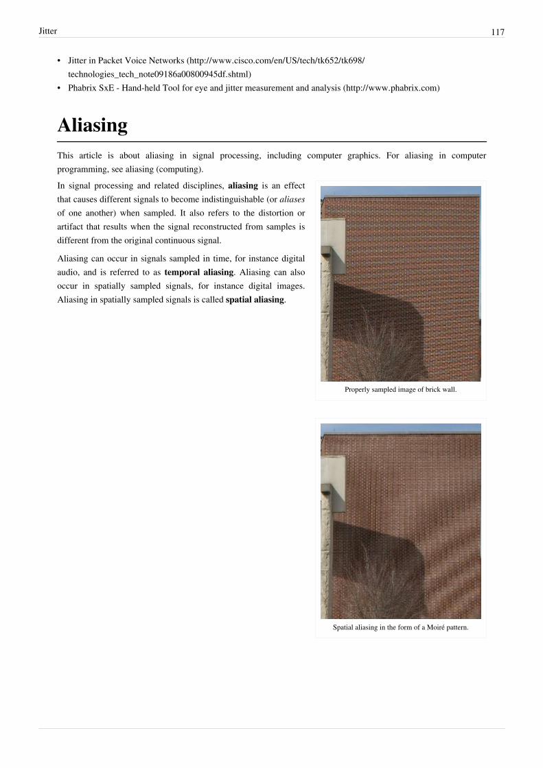
Jitter 117
• Jitter in Packet Voice Networks (http:/ / www. cisco. com/ en/ US/ tech/ tk652/ tk698/technologies_tech_note09186a00800945df. shtml)
• Phabrix SxE - Hand-held Tool for eye and jitter measurement and analysis (http:/ / www. phabrix. com)
AliasingThis article is about aliasing in signal processing, including computer graphics. For aliasing in computerprogramming, see aliasing (computing).
Properly sampled image of brick wall.
Spatial aliasing in the form of a Moiré pattern.
In signal processing and related disciplines, aliasing is an effectthat causes different signals to become indistinguishable (or aliasesof one another) when sampled. It also refers to the distortion orartifact that results when the signal reconstructed from samples isdifferent from the original continuous signal.
Aliasing can occur in signals sampled in time, for instance digitalaudio, and is referred to as temporal aliasing. Aliasing can alsooccur in spatially sampled signals, for instance digital images.Aliasing in spatially sampled signals is called spatial aliasing.

Aliasing 118
Description
Aliasing example of the A letter in Times New Roman.Left: aliased image, right: anti-aliased image.
When a digital image is viewed, a reconstruction is performed by adisplay or printer device, and by the eyes and the brain. If theimage data is not properly processed during sampling orreconstruction, the reconstructed image will differ from theoriginal image, and an alias is seen.
An example of spatial aliasing is the Moiré pattern one canobserve in a poorly pixelized image of a brick wall. Techniquesthat avoid such poor pixelizations are called spatial anti-aliasing.Aliasing can be caused either by the sampling stage or thereconstruction stage; these may be distinguished by calling sampling aliasing prealiasing and reconstruction aliasingpostaliasing.
Temporal aliasing is a major concern in the sampling of video and audio signals. Music, for instance, may containhigh-frequency components that are inaudible to humans. If a piece of music is sampled at 32000 samples per second(Hz), any frequency components above 16000 Hz (the Nyquist frequency) will cause aliasing when the music isreproduced by a digital to analog converter (DAC). To prevent this an anti-aliasing filter is used to removecomponents above the Nyquist frequency prior to sampling.In video or cinematography, temporal aliasing results from the limited frame rate, and causes the wagon-wheeleffect, whereby a spoked wheel appears to rotate too slowly or even backwards. Aliasing has changed its apparentfrequency of rotation. A reversal of direction can be described as a negative frequency. Temporal aliasingfrequencies in video and cinematography are determined by the frame rate of the camera, but the relative intensity ofthe aliased frequencies is determined by the shutter timing (exposure time) or the use of a temporal aliasingreduction filter during filming.[1]
Like the video camera, most sampling schemes are periodic; that is, they have a characteristic sampling frequency intime or in space. Digital cameras provide a certain number of samples (pixels) per degree or per radian, or samplesper mm in the focal plane of the camera. Audio signals are sampled (digitized) with an analog-to-digital converter,which produces a constant number of samples per second. Some of the most dramatic and subtle examples ofaliasing occur when the signal being sampled also has periodic content.
Bandlimited functionsMain article: Nyquist–Shannon sampling theoremActual signals have finite duration and their frequency content, as defined by the Fourier transform, has no upperbound. Some amount of aliasing always occurs when such functions are sampled. Functions whose frequencycontent is bounded (bandlimited) have infinite duration. If sampled at a high enough rate, determined by thebandwidth, the original function can in theory be perfectly reconstructed from the infinite set of samples.
Bandpass signalsMain article: UndersamplingSometimes aliasing is used intentionally on signals with no low-frequency content, called bandpass signals.Undersampling, which creates low-frequency aliases, can produce the same result, with less effort, asfrequency-shifting the signal to lower frequencies before sampling at the lower rate. Some digital channelizersexploit aliasing in this way for computational efficiency. See Sampling (signal processing), Nyquist rate (relative tosampling), and Filter bank.

Aliasing 119
Sampling sinusoidal functionsSinusoids are an important type of periodic function, because realistic signals are often modeled as the summation ofmany sinusoids of different frequencies and different amplitudes (with a Fourier series or transform). Understandingwhat aliasing does to the individual sinusoids is useful in understanding what happens to their sum.
Two different sinusoids that fit the same set of samples.
Here, a plot depicts a set of samples whosesample-interval is 1, and two (of many)different sinusoids that could have producedthe samples. The sample-rate in this case is
. For instance, if the interval is 1second, the rate is 1 sample per second.Nine cycles of the red sinusoid and 1 cycleof the blue sinusoid span an interval of 10.The respective sinusoid frequencies are
and . In general, when a sinusoid of frequency is sampled with frequency theresulting samples are indistinguishable from those of another sinusoid of frequency for any integer N.The values corresponding to N ≠ 0 are called images or aliases of frequency In our example, the N = ±1 aliasesof are and A negative frequency is equivalent to its absolute value,because sin(−wt + θ) = sin(wt − θ + π), and cos(−wt + θ) = cos(wt − θ). Therefore we can express all the imagefrequencies as for any integer N (with being the actual signal frequency).Then the N = 1 alias of is (and vice versa).Aliasing matters when one attempts to reconstruct the original waveform from its samples. The most commonreconstruction technique produces the smallest of the frequencies. So it is usually important that
be the unique minimum. A necessary and sufficient condition for that is where iscommonly called the Nyquist frequency of a system that samples at rate In our example, the Nyquist conditionis satisfied if the original signal is the blue sinusoid ( ). But if the usual reconstruction methodwill produce the blue sinusoid instead of the red one.
The black dots are aliases of each other. The solid red line is an example ofadjusting amplitude vs frequency. The dashed red lines are the corresponding paths
of the aliases.
Folding
In the example above, and aresymmetrical around the frequency And in general, as increases from 0 to
decreases from to Similarly, as increases from
to continues decreasing fromto 0.
A graph of amplitude vs frequency for asingle sinusoid at frequency and someof its aliases at and wouldlook like the 4 black dots in the adjacentfigure. The red lines depict the paths (loci) of the 4 dots if we were to adjust the frequency and amplitude of thesinusoid along the solid red segment (between and ). No matter what function we choose to change theamplitude vs frequency, the graph will exhibit symmetry between 0 and This symmetry is commonly referred toas folding, and another name for (the Nyquist frequency) is folding frequency. Folding is most often observedin practice when viewing the frequency spectrum of real-valued samples using a discrete Fourier transform.

Aliasing 120
Two complex sinusoids, colored gold and cyan, that fit the same sets of real andimaginary sample points when sampled at the rate (fs) indicated by the grid lines.
The case shown here is:
Complex sinusoids
Complex sinusoids are waveforms whosesamples are complex numbers, and theconcept of negative frequency is necessaryto distinguish them. In that case, thefrequencies of the aliases are given by just:
Therefore, asincreases from to
goes from up to 0. Consequently,complex sinusoids do not exhibit folding.Complex samples of real-valued sinusoidshave zero-valued imaginary parts and doexhibit folding.
Sample frequency
Illustration of 4 waveforms reconstructed from samples taken at six different rates.Two of the waveforms are sufficiently sampled to avoid aliasing at all six rates.
The other two illustrate increasing distortion (aliasing) at the lower rates.
When the condition is met for thehighest frequency component of the originalsignal, then it is met for all the frequencycomponents, a condition known as theNyquist criterion. That is typicallyapproximated by filtering the original signalto attenuate high frequency componentsbefore it is sampled. They still generatelow-frequency aliases, but at very lowamplitude levels, so as not to cause aproblem. A filter chosen in anticipation of acertain sample frequency is called ananti-aliasing filter. The filtered signal cansubsequently be reconstructed withoutsignificant additional distortion, for exampleby the Whittaker–Shannon interpolationformula.
The Nyquist criterion presumes that the frequency content of the signal being sampled has an upper bound. Implicitin that assumption is that the signal's duration has no upper bound. Similarly, the Whittaker–Shannon interpolationformula represents an interpolation filter with an unrealizable frequency response. These assumptions make up amathematical model that is an idealized approximation, at best, to any realistic situation. The conclusion, that perfectreconstruction is possible, is mathematically correct for the model, but only an approximation for actual samples ofan actual signal.

Aliasing 121
Historical usageHistorically the term aliasing evolved from radio engineering because of the action of superheterodyne receivers.When the receiver shifts multiple signals down to lower frequencies, from RF to IF by heterodyning, an unwantedsignal, from an RF frequency equally far from the local oscillator (LO) frequency as the desired signal, but on thewrong side of the LO, can end up at the same IF frequency as the wanted one. If it is strong enough it can interferewith reception of the desired signal. This unwanted signal is known as an image or alias of the desired signal.
Angular aliasingAliasing occurs whenever the use of discrete elements to capture or produce a continuous signal causes frequencyambiguity.Spatial aliasing, particular of angular frequency, can occur when reproducing a light field[2] or sound field withdiscrete elements, as in 3D displays or wave field synthesis of sound.This aliasing is visible in images such as posters with lenticular printing: if they have low angular resolution, then asone moves past them, say from left-to-right, the 2D image does not initially change (so it appears to move left), thenas one moves to the next angular image, the image suddenly changes (so it jumps right) – and the frequency andamplitude of this side-to-side movement corresponds to the angular resolution of the image (and, for frequency, thespeed of the viewer's lateral movement), which is the angular aliasing of the 4D light field.The lack of parallax on viewer movement in 2D images and in 3-D film produced by stereoscopic glasses (in 3Dfilms the effect is called "yawing", as the image appears to rotate on its axis) can similarly be seen as loss of angularresolution, all angular frequencies being aliased to 0 (constant).
More examples
Online audio exampleThe qualitative effects of aliasing can be heard in the following audio demonstration. Six sawtooth waves are playedin succession, with the first two sawtooths having a fundamental frequency of 440 Hz (A4), the second two havingfundamental frequency of 880 Hz (A5), and the final two at 1760 Hz (A6). The sawtooths alternate betweenbandlimited (non-aliased) sawtooths and aliased sawtooths and the sampling rate is 22.05 kHz. The bandlimitedsawtooths are synthesized from the sawtooth waveform's Fourier series such that no harmonics above the Nyquistfrequency are present.The aliasing distortion in the lower frequencies is increasingly obvious with higher fundamental frequencies, andwhile the bandlimited sawtooth is still clear at 1760 Hz, the aliased sawtooth is degraded and harsh with a buzzingaudible at frequencies lower than the fundamental.
Sawtooth aliasing demo
440 Hz bandlimited, 440 Hz aliased, 880 Hz bandlimited, 880 Hz aliased, 1760 Hz bandlimited, 1760 Hz aliased
Problems playing this file? See media help.

Aliasing 122
Direction findingA form of spatial aliasing can also occur in antenna arrays or microphone arrays used to estimate the direction ofarrival of a wave signal, as in geophysical exploration by seismic waves. Waves must be sampled at more than twopoints per wavelength, or the wave arrival direction becomes ambiguous.[3]
Further reading"Sampling and reconstruction," Chapter 7 [4] in.
References[1] Tessive, LLC (2010). "Time Filter Technical Explanation" (http:/ / tessive. com/ time-filter-technical-explanation)[2] The (New) Stanford Light Field Archive (http:/ / lightfield. stanford. edu/ lfs. html)[3] Flanagan J.L., ‘Beamwidth and useable bandwidth of delay- steered microphone arrays’, AT&T Tech. J., 1985, 64, pp. 983–995[4] http:/ / graphics. stanford. edu/ ~mmp/ chapters/ pbrt_chapter7. pdf
External links• Aliasing by a sampling oscilloscope (http:/ / www. youtube. com/ watch?v=g3svU5VJ8Gk& feature=plcp) by
Tektronix Application Engineer• Anti-Aliasing Filter Primer (http:/ / lavidaleica. com/ content/ anti-aliasing-filter-primer)Wikipedia:Link rot by La
Vida Leica discusses its purpose and effect on the image recorded.• Frequency Aliasing Demonstration (http:/ / burtonmackenzie. com/ 2006/ 07/ i-cant-drive-55. html) by Burton
MacKenZie using stop frame animation and a clock.• Interactive examples demonstrating the aliasing effect (http:/ / www. onmyphd. com/ ?p=aliasing)
Anti-aliasing filterAn anti-aliasing filter is a filter used before a signal sampler, to restrict the bandwidth of a signal to approximatelysatisfy the sampling theorem. Since the theorem states that unambiguous interpretation of the signal from its samplesis possible when the power of frequencies above the Nyquist frequency is zero, a real anti-aliasing filter cangenerally not completely satisfy the theorem. A realizable anti-aliasing filter will typically permit some aliasing tooccur; the amount of aliasing that does occur depends on a design trade-off between reduction of aliasing andmaintaining signal up to the Nyquist frequency and the frequency content of the input signal.
Optical applicationsIn the case of optical image sampling, as by image sensors in digital cameras, the anti-aliasing filter is also known asan optical lowpass filter or blur filter or AA filter. The mathematics of sampling in two spatial dimensions is similarto the mathematics of time-domain sampling, but the filter implementation technologies are different. The typicalimplementation in digital cameras is two layers of birefringent material such as lithium niobate, which spreads eachoptical point into a cluster of four points.The choice of spot separation for such a filter involves a tradeoff among sharpness, aliasing, and fill factor (the ratioof the active refracting area of a microlens array to the total contiguous area occupied by the array). In amonochrome or three-CCD or Foveon X3 camera, the microlens array alone, if near 100% effective, can provide asignificant anti-aliasing effect, while in color filter array (CFA, e.g. Bayer filter) cameras, an additional filter isgenerally needed to reduce aliasing to an acceptable level.

Anti-aliasing filter 123
Sensor based anti-aliasing filter simulationThe Pentax K-3 from Ricoh introduced a unique digital sensor based anti-aliasing filter. The filter works by microvibrating the sensor element. A toggle can on-off anti-aliasing filter as the world's first camera which has itscapability.
Audio applicationsAnti-aliasing filters are commonly used at the input of digital signal processing systems, for example in sounddigitization systems; similar filters are used as reconstruction filters at the output of such systems, for example inmusic players. In the latter case, the filter functions to prevent aliasing in the conversion of samples back to acontinuous signal, where again perfect stop-band rejection would be required to guarantee zero aliasing.
OversamplingA technique known as oversampling is commonly used in audio conversion, especially audio output. The idea is touse a higher intermediate digital sample rate, so that a nearly-ideal digital filter can sharply cut off aliasing near theoriginal low Nyquist frequency, while a much simpler analog filter can stop frequencies above the new higherNyquist frequency.The purpose of oversampling is to relax the requirements on the anti-aliasing filter, or to further reduce the aliasing.Since the initial anti-aliasing filter is analog, oversampling allows for the filter to be cheaper because therequirements are not as stringent, and also allows the anti-aliasing filter to have a smoother frequency response, andthus a less complex phase response.On input, an initial analog anti-aliasing filter is relaxed, the signal is sampled at a high rate, and then downsampledusing a nearly ideal digital anti-aliasing filter.
Bandpass signalsSee also: UndersamplingOften, an anti-aliasing filter is a low-pass filter; however, this is not a requirement. Generalizations of theNyquist–Shannon sampling theorem allow sampling of other band-limited passband signals instead of basebandsignals.For signals that are bandwidth limited, but not centered at zero, a band-pass filter can be used as an anti-aliasingfilter. For example, this could be done with a single-sideband modulated or frequency modulated signal. If onedesired to sample an FM radio broadcast centered at 87.9 MHz and bandlimited to a 200 kHz band, then anappropriate anti-alias filter would be centered on 87.9 MHz with 200 kHz bandwidth (or pass-band of 87.8 MHz to88.0 MHz), and the sampling rate would be no less than 400 kHz, but should also satisfy other constraints to preventaliasing.
Signal overloadSee also: Clipping (audio)It is very important to avoid input signal overload when using an anti-aliasing filter. If the signal is strong enough, itcan cause clipping at the analog-to-digital converter, even after filtering. When distortion due to clipping occurs afterthe anti-aliasing filter, it can create components outside the passband of the anti-aliasing filter; these components canthen alias, causing the reproduction of other non-harmonically-related frequencies.

Anti-aliasing filter 124
References
Flash ADCA Flash ADC (also known as a Direct conversion ADC) is a type of analog-to-digital converter that uses a linearvoltage ladder with a comparator at each "rung" of the ladder to compare the input voltage to successive referencevoltages. Often these reference ladders are constructed of many resistors; however modern implementations showthat capacitive voltage division is also possible. The output of these comparators is generally fed into a digitalencoder which converts the inputs into a binary value (the collected outputs from the comparators can be thought ofas a unary value).
Benefits and drawbacksFlash converters are extremely fast compared to many other types of ADCs which usually narrow in on the "correct"answer over a series of stages. Compared to these, a Flash converter is also quite simple and, apart from the analogcomparators, only requires logic for the final conversion to binary.For best accuracy often a track-and-hold circuit is inserted in front of the ADC input. This is needed for many ADCtypes (like successive approximation ADC), but for Flash ADCs there is no real need for this, because thecomparators are the sampling devices.A Flash converter requires a huge number of comparators compared to other ADCs, especially as the precisionincreases. A Flash converter requires comparators for an n-bit conversion. The size, power consumption andcost of all those comparators makes Flash converters generally impractical for precisions much greater than 8 bits(255 comparators). In place of these comparators, most other ADCs substitute more complex logic and/or analogcircuitry which can be scaled more easily for increased precision.

Flash ADC 125
Implementation
A 2-bit Flash ADC Example Implementation with Bubble Error Correction and DigitalEncoding
Flash ADCs have been implemented inmany technologies, varying fromsilicon based bipolar (BJT) andcomplementary metal oxide FETs(CMOS) technologies to rarely usedIII-V technologies. Often this type ofADC is used as a first medium sizedanalog circuit verification.
The earliest implementations consistedof a reference ladder of well matchedresistors connected to a referencevoltage. Each tap at the resistor ladderis used for one comparator, possiblypreceded by an amplification stage,and thus generates a logical '0' or '1'depending if the measured voltage isabove or below the reference voltageof the resistor tap. The reason to add anamplifier is twofold: it amplifies thevoltage difference and thereforesuppresses the comparator offset, andthe kick-back noise of the comparatortowards the reference ladder is also strongly suppressed. Typically designs from 4-bit up to 6-bit, and sometimes7-bit are produced.Designs with power-saving capacitive reference ladders have been demonstrated. In addition to clocking thecomparator(s), these systems also sample the reference value on the input stage. As the sampling is done at a veryhigh rate, the leakage of the capacitors is negligible.Recently, offset calibration has been introduced into flash ADC designs. Instead of high precision analog circuits(which increase component size to suppress variation) comparators with relatively large offset errors are measuredand adjusted. A test signal is applied and the offset of each comparator is calibrated to below the LSB size of theADC.Another improvement to many flash ADCs is the inclusion of digital error correction. When the ADC is used inharsh environments or constructed from very small integrated circuit processes, there is a heightened risk a singlecomparator will randomly change state resulting in a wrong code. Bubble error correction is a digital correctionmechanism that will prevent a comparator that has, for example, tripped high from reporting logic high if it issurrounded by comparators that are reporting logic low.
Folding ADCThe number of comparators can be reduced somewhat by adding a folding circuit in front, making a so called foldingADC. Instead of using the comparators in a Flash ADC only once, during a ramp input signal, the folding ADCre-uses the comparators multiple times. If a m-times folding circuit is used in an n-bit ADC, the actual number ofcomparator can be reduced from to (there is always one needed to detect the range crossover). Typicalfolding circuits are, e.g., the Gilbert multiplier, or analog wired-or circuits.
Flash ADC 126
ApplicationThe very high sample rate of this type of ADC enable gigahertz applications like radar detection, wide band radioreceivers and optical communication links. More often the flash ADC is embedded in a large IC containing manydigital decoding functions.Also a small flash ADC circuit may be present inside a delta-sigma modulation loop.Flash ADCs are also used in NAND Flash Memory, where up to 3 bits are stored per cell as 8 level voltages onfloating gates.
References• Analog to Digital Conversion [1]
• Understanding Flash ADCs [2]
•• "Integrated Analog-to-Digital and Digital-to-Analog Converters ", R. van de Plassche, ADCs, Kluwer AcademicPublishers, 1994.
•• "A Precise Four-Quadrant Multiplier with Subnanosecond Response", Barrie Gilbert, IEEE Journal of Solid-StateCircuits, Vol. 3, No. 4 (1968), pp. 365-373
References[1] http:/ / hyperphysics. phy-astr. gsu. edu/ hbase/ electronic/ adc. html#c4[2] http:/ / www. maxim-ic. com/ appnotes. cfm/ appnote_number/ 810/ CMP/ WP-17
Successive approximation ADC"Successive Approximation" redirects here. For behaviorist B.F. Skinner's method of guiding learned behavior, seeShaping (psychology).A successive approximation ADC is a type of analog-to-digital converter that converts a continuous analogwaveform into a discrete digital representation via a binary search through all possible quantization levels beforefinally converging upon a digital output for each conversion.

Successive approximation ADC 127
Block diagram
Successive Approximation ADC Block Diagram
Key
•• DAC = Digital-to-Analog converter•• EOC = end of conversion•• SAR = successive approximation register•• S/H = sample and hold circuit• Vin = input voltage• Vref = reference voltage
Algorithm
The successive approximation Analog todigital converter circuit typically consists offour chief subcircuits:
1. A sample and hold circuit to acquirethe input voltage (Vin).
2. An analog voltage comparator thatcompares Vin to the output of theinternal DAC and outputs the result of the comparison to the successive approximation register (SAR).
3. A successive approximation register subcircuit designed to supply an approximate digital code of Vin to theinternal DAC.
4. An internal reference DAC that, for comparison with V, supplies the comparator with an analog voltage equalto the digital code output of the SARin.
The successive approximation register is initialized so that the most significant bit (MSB) is equal to a digital 1. Thiscode is fed into the DAC, which then supplies the analog equivalent of this digital code (Vref/2) into the comparatorcircuit for comparison with the sampled input voltage. If this analog voltage exceeds Vin the comparator causes theSAR to reset this bit; otherwise, the bit is left a 1. Then the next bit is set to 1 and the same test is done, continuingthis binary search until every bit in the SAR has been tested. The resulting code is the digital approximation of thesampled input voltage and is finally output by the SAR at the end of the conversion (EOC).Mathematically, let Vin = xVref, so x in [-1, 1] is the normalized input voltage. The objective is to approximatelydigitize x to an accuracy of 1/2n. The algorithm proceeds as follows:
1. Initial approximation x0 = 0.2. ith approximation xi = xi-1 - s(xi-1 - x)/2i.
where, s(x) is the signum-function(sgn(x)) (+1 for x ≥ 0, -1 for x < 0). It follows using mathematical induction that|xn - x| ≤ 1/2n.As shown in the above algorithm, a SAR ADC requires:
1. An input voltage source Vin.2. A reference voltage source Vref to normalize the input.3. A DAC to convert the ith approximation xi to a voltage.4. A Comparator to perform the function s(xi - x) by comparing the DAC's voltage with the input voltage.5. A Register to store the output of the comparator and apply xi-1 - s(xi-1 - x)/2i.
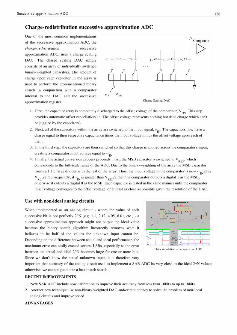
Successive approximation ADC 128
Charge-redistribution successive approximation ADC
Charge Scaling DAC
One of the most common implementationsof the successive approximation ADC, thecharge-redistribution successiveapproximation ADC, uses a charge scalingDAC. The charge scaling DAC simplyconsists of an array of individually switchedbinary-weighted capacitors. The amount ofcharge upon each capacitor in the array isused to perform the aforementioned binarysearch in conjunction with a comparatorinternal to the DAC and the successiveapproximation register.
1. First, the capacitor array is completely discharged to the offset voltage of the comparator, VOS. This stepprovides automatic offset cancellation(i.e. The offset voltage represents nothing but dead charge which can'tbe juggled by the capacitors).
2. Next, all of the capacitors within the array are switched to the input signal, vIN. The capacitors now have acharge equal to their respective capacitance times the input voltage minus the offset voltage upon each ofthem.
3. In the third step, the capacitors are then switched so that this charge is applied across the comparator's input,creating a comparator input voltage equal to -vIN.
4. Finally, the actual conversion process proceeds. First, the MSB capacitor is switched to VREF, whichcorresponds to the full-scale range of the ADC. Due to the binary-weighting of the array the MSB capacitorforms a 1:1 charge divider with the rest of the array. Thus, the input voltage to the comparator is now -vIN plusVREF/2. Subsequently, if vIN is greater than VREF/2 then the comparator outputs a digital 1 as the MSB,otherwise it outputs a digital 0 as the MSB. Each capacitor is tested in the same manner until the comparatorinput voltage converges to the offset voltage, or at least as close as possible given the resolution of the DAC.
3 bits simulation of a capacitive ADC
Use with non-ideal analog circuits
When implemented as an analog circuit - where the value of eachsuccessive bit is not perfectly 2^N (e.g. 1.1, 2.12, 4.05, 8.01, etc.) - asuccessive approximation approach might not output the ideal valuebecause the binary search algorithm incorrectly removes what itbelieves to be half of the values the unknown input cannot be.Depending on the difference between actual and ideal performance, themaximum error can easily exceed several LSBs, especially as the errorbetween the actual and ideal 2^N becomes large for one or more bits.Since we don't know the actual unknown input, it is therefore veryimportant that accuracy of the analog circuit used to implement a SAR ADC be very close to the ideal 2^N values;otherwise, we cannot guarantee a best match search.RECENT IMPROVEMENTS
1.1. New SAR ADC include now calibration to improve their accuracy from less than 10bits to up to 18bits2.2. Another new technique use non-binary weighted DAC and/or redundancy to solve the problem of non-ideal
analog circuits and improve speedADVANTAGES
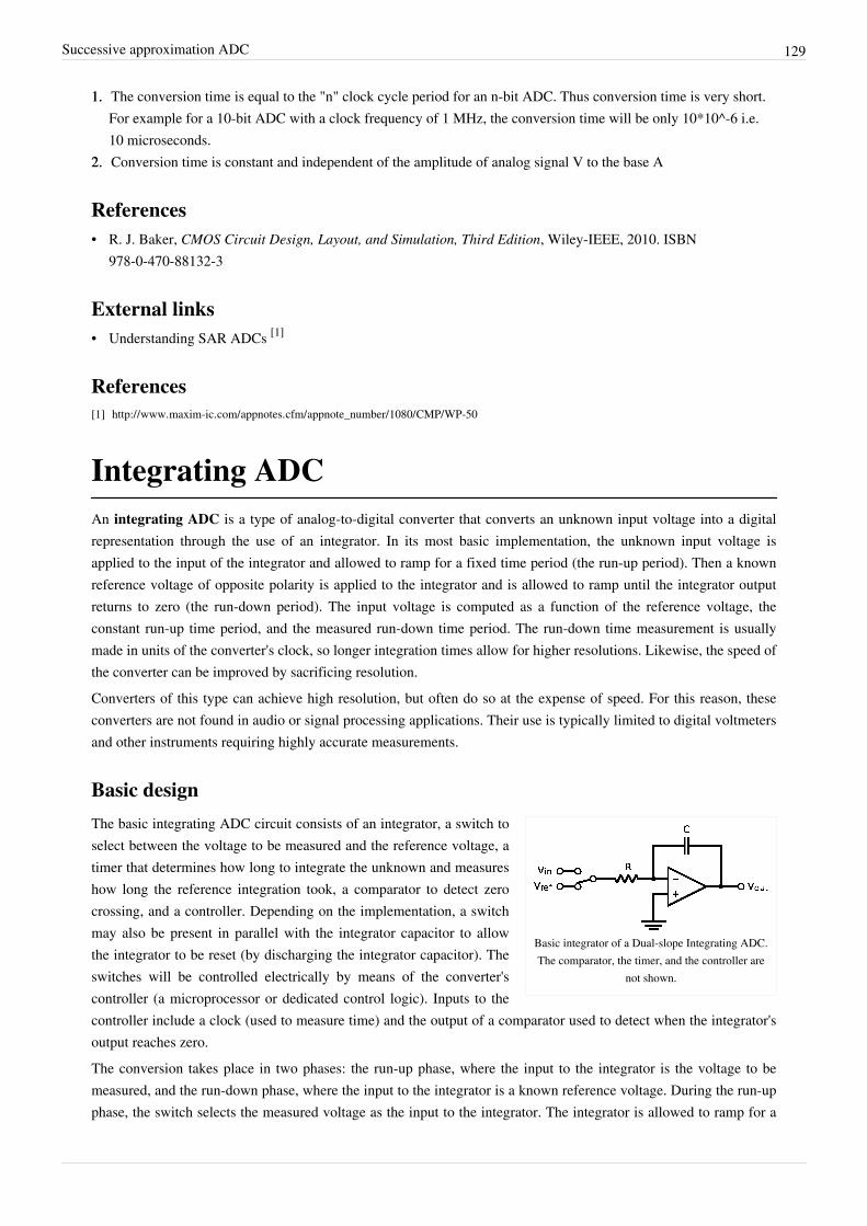
Successive approximation ADC 129
1.1. The conversion time is equal to the "n" clock cycle period for an n-bit ADC. Thus conversion time is very short.For example for a 10-bit ADC with a clock frequency of 1 MHz, the conversion time will be only 10*10^-6 i.e.10 microseconds.
2.2. Conversion time is constant and independent of the amplitude of analog signal V to the base A
References• R. J. Baker, CMOS Circuit Design, Layout, and Simulation, Third Edition, Wiley-IEEE, 2010. ISBN
978-0-470-88132-3
External links• Understanding SAR ADCs [1]
References[1] http:/ / www. maxim-ic. com/ appnotes. cfm/ appnote_number/ 1080/ CMP/ WP-50
Integrating ADCAn integrating ADC is a type of analog-to-digital converter that converts an unknown input voltage into a digitalrepresentation through the use of an integrator. In its most basic implementation, the unknown input voltage isapplied to the input of the integrator and allowed to ramp for a fixed time period (the run-up period). Then a knownreference voltage of opposite polarity is applied to the integrator and is allowed to ramp until the integrator outputreturns to zero (the run-down period). The input voltage is computed as a function of the reference voltage, theconstant run-up time period, and the measured run-down time period. The run-down time measurement is usuallymade in units of the converter's clock, so longer integration times allow for higher resolutions. Likewise, the speed ofthe converter can be improved by sacrificing resolution.Converters of this type can achieve high resolution, but often do so at the expense of speed. For this reason, theseconverters are not found in audio or signal processing applications. Their use is typically limited to digital voltmetersand other instruments requiring highly accurate measurements.
Basic design
Basic integrator of a Dual-slope Integrating ADC.The comparator, the timer, and the controller are
not shown.
The basic integrating ADC circuit consists of an integrator, a switch toselect between the voltage to be measured and the reference voltage, atimer that determines how long to integrate the unknown and measureshow long the reference integration took, a comparator to detect zerocrossing, and a controller. Depending on the implementation, a switchmay also be present in parallel with the integrator capacitor to allowthe integrator to be reset (by discharging the integrator capacitor). Theswitches will be controlled electrically by means of the converter'scontroller (a microprocessor or dedicated control logic). Inputs to thecontroller include a clock (used to measure time) and the output of a comparator used to detect when the integrator'soutput reaches zero.The conversion takes place in two phases: the run-up phase, where the input to the integrator is the voltage to bemeasured, and the run-down phase, where the input to the integrator is a known reference voltage. During the run-upphase, the switch selects the measured voltage as the input to the integrator. The integrator is allowed to ramp for a
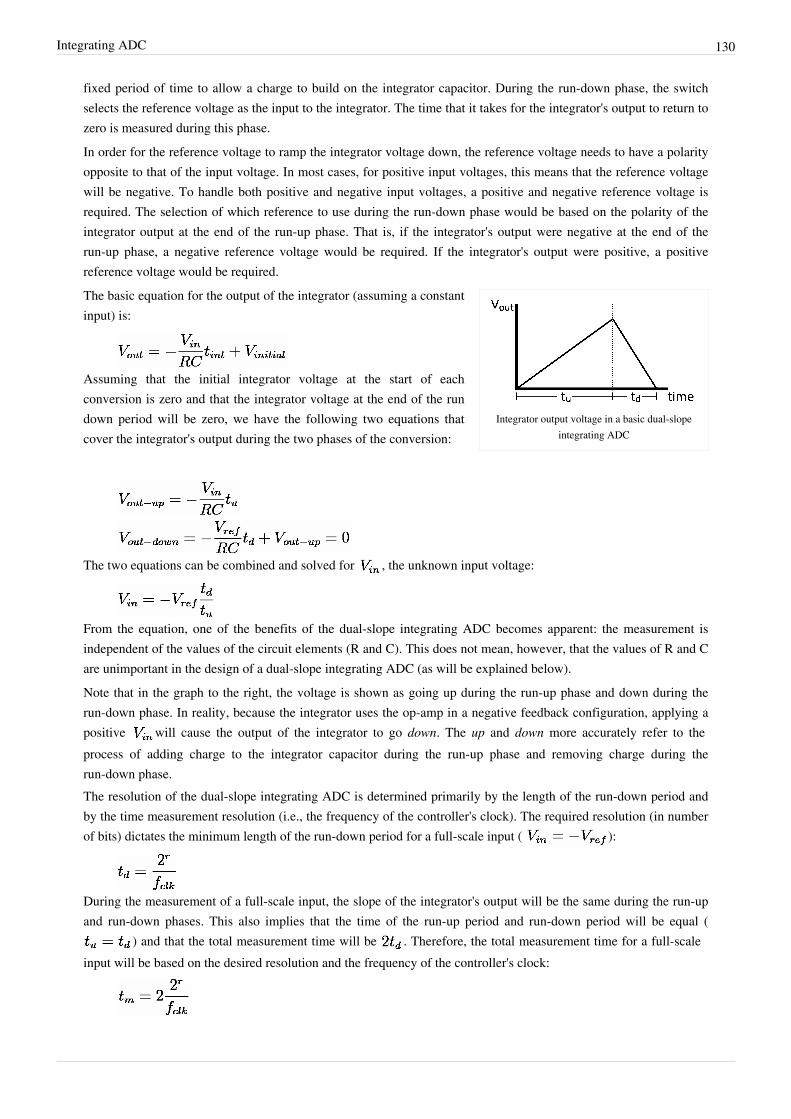
Integrating ADC 130
fixed period of time to allow a charge to build on the integrator capacitor. During the run-down phase, the switchselects the reference voltage as the input to the integrator. The time that it takes for the integrator's output to return tozero is measured during this phase.In order for the reference voltage to ramp the integrator voltage down, the reference voltage needs to have a polarityopposite to that of the input voltage. In most cases, for positive input voltages, this means that the reference voltagewill be negative. To handle both positive and negative input voltages, a positive and negative reference voltage isrequired. The selection of which reference to use during the run-down phase would be based on the polarity of theintegrator output at the end of the run-up phase. That is, if the integrator's output were negative at the end of therun-up phase, a negative reference voltage would be required. If the integrator's output were positive, a positivereference voltage would be required.
Integrator output voltage in a basic dual-slopeintegrating ADC
The basic equation for the output of the integrator (assuming a constantinput) is:
Assuming that the initial integrator voltage at the start of eachconversion is zero and that the integrator voltage at the end of the rundown period will be zero, we have the following two equations thatcover the integrator's output during the two phases of the conversion:
The two equations can be combined and solved for , the unknown input voltage:
From the equation, one of the benefits of the dual-slope integrating ADC becomes apparent: the measurement isindependent of the values of the circuit elements (R and C). This does not mean, however, that the values of R and Care unimportant in the design of a dual-slope integrating ADC (as will be explained below).Note that in the graph to the right, the voltage is shown as going up during the run-up phase and down during therun-down phase. In reality, because the integrator uses the op-amp in a negative feedback configuration, applying apositive will cause the output of the integrator to go down. The up and down more accurately refer to theprocess of adding charge to the integrator capacitor during the run-up phase and removing charge during therun-down phase.The resolution of the dual-slope integrating ADC is determined primarily by the length of the run-down period andby the time measurement resolution (i.e., the frequency of the controller's clock). The required resolution (in numberof bits) dictates the minimum length of the run-down period for a full-scale input ( ):
During the measurement of a full-scale input, the slope of the integrator's output will be the same during the run-upand run-down phases. This also implies that the time of the run-up period and run-down period will be equal (
) and that the total measurement time will be . Therefore, the total measurement time for a full-scaleinput will be based on the desired resolution and the frequency of the controller's clock:
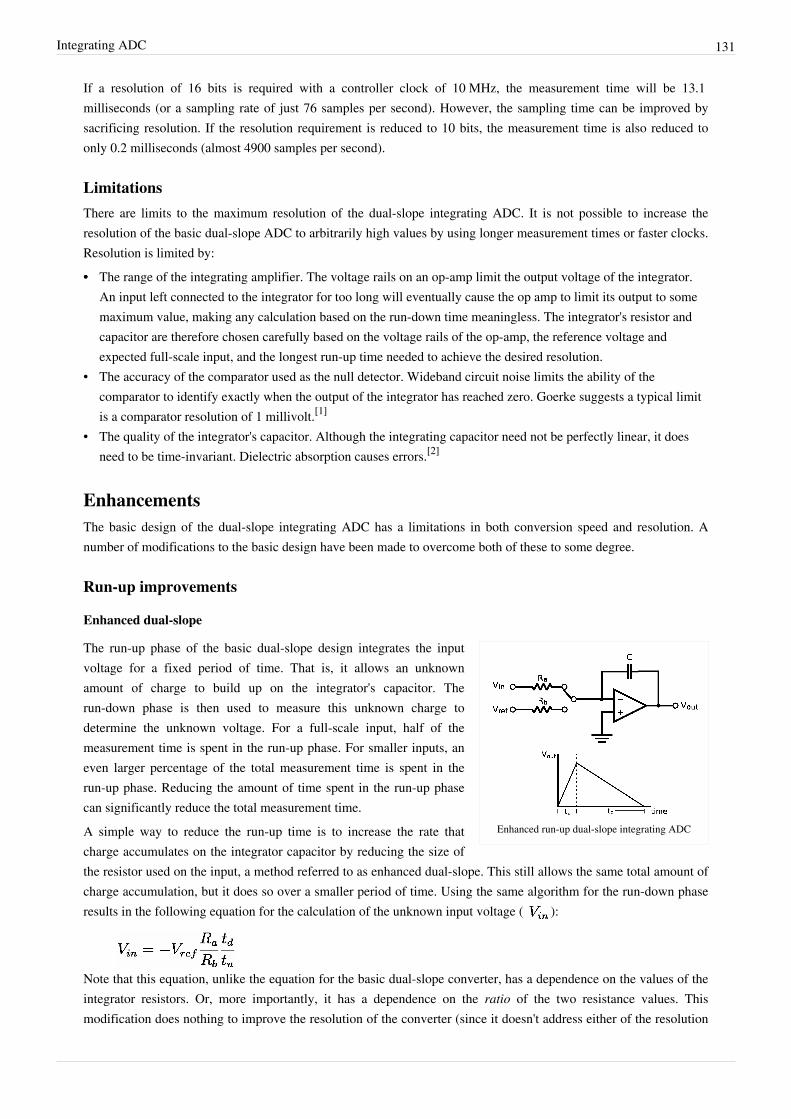
Integrating ADC 131
If a resolution of 16 bits is required with a controller clock of 10 MHz, the measurement time will be 13.1milliseconds (or a sampling rate of just 76 samples per second). However, the sampling time can be improved bysacrificing resolution. If the resolution requirement is reduced to 10 bits, the measurement time is also reduced toonly 0.2 milliseconds (almost 4900 samples per second).
LimitationsThere are limits to the maximum resolution of the dual-slope integrating ADC. It is not possible to increase theresolution of the basic dual-slope ADC to arbitrarily high values by using longer measurement times or faster clocks.Resolution is limited by:•• The range of the integrating amplifier. The voltage rails on an op-amp limit the output voltage of the integrator.
An input left connected to the integrator for too long will eventually cause the op amp to limit its output to somemaximum value, making any calculation based on the run-down time meaningless. The integrator's resistor andcapacitor are therefore chosen carefully based on the voltage rails of the op-amp, the reference voltage andexpected full-scale input, and the longest run-up time needed to achieve the desired resolution.
• The accuracy of the comparator used as the null detector. Wideband circuit noise limits the ability of thecomparator to identify exactly when the output of the integrator has reached zero. Goerke suggests a typical limitis a comparator resolution of 1 millivolt.[1]
• The quality of the integrator's capacitor. Although the integrating capacitor need not be perfectly linear, it doesneed to be time-invariant. Dielectric absorption causes errors.[2]
EnhancementsThe basic design of the dual-slope integrating ADC has a limitations in both conversion speed and resolution. Anumber of modifications to the basic design have been made to overcome both of these to some degree.
Run-up improvements
Enhanced dual-slope
Enhanced run-up dual-slope integrating ADC
The run-up phase of the basic dual-slope design integrates the inputvoltage for a fixed period of time. That is, it allows an unknownamount of charge to build up on the integrator's capacitor. Therun-down phase is then used to measure this unknown charge todetermine the unknown voltage. For a full-scale input, half of themeasurement time is spent in the run-up phase. For smaller inputs, aneven larger percentage of the total measurement time is spent in therun-up phase. Reducing the amount of time spent in the run-up phasecan significantly reduce the total measurement time.A simple way to reduce the run-up time is to increase the rate thatcharge accumulates on the integrator capacitor by reducing the size ofthe resistor used on the input, a method referred to as enhanced dual-slope. This still allows the same total amount ofcharge accumulation, but it does so over a smaller period of time. Using the same algorithm for the run-down phaseresults in the following equation for the calculation of the unknown input voltage ( ):
Note that this equation, unlike the equation for the basic dual-slope converter, has a dependence on the values of the integrator resistors. Or, more importantly, it has a dependence on the ratio of the two resistance values. This modification does nothing to improve the resolution of the converter (since it doesn't address either of the resolution

Integrating ADC 132
limitations noted above).
Multi-slope run-up
Circuit diagram for a multi-slope run-upconverter
One method to improve the resolution of the converter is to artificiallyincrease the range of the integrating amplifier during the run-up phase.As mentioned above, the purpose of the run-up phase is to add anunknown amount of charge to the integrator to be later measuredduring the run-down phase. Having the ability to add larger quantitiesof charge allows for more higher-resolution measurements. Forexample, assume that we are capable of measuring the charge on theintegrator during the run-down phase to a granularity of 1 coulomb. Ifour integrator amplifier limits us to being able to add only up to 16 coulombs of charge to the integrator during therun-up phase, our total measurement will be limited to 4 bits (16 possible values). If we can increase the range of theintegrator to allow us to add up to 32 coulombs, our measurement resolution is increased to 5 bits.One method to increase the integrator capacity is by periodically adding or subtracting known quantities of chargeduring the run-up phase in order to keep the integrator's output within the range of the integrator amplifier. Then, thetotal amount of artificially-accumulated charge is the charge introduced by the unknown input voltage plus the sumof the known charges that were added or subtracted.The circuit diagram shown to the right is an example of how multi-slope run-up could be implemented. The conceptis that the unknown input voltage, , is always applied to the integrator. Positive and negative reference voltagescontrolled by the two independent switches add and subtract charge as needed to keep the output of the integratorwithin its limits. The reference resistors, and are necessarily smaller than to ensure that the referencescan overcome the charge introduced by the input. A comparator is connected to the output to compare the integrator'svoltage with a threshold voltage. The output of the comparator is used by the converter's controller to decide whichreference voltage should be applied. This can be a relatively simple algorithm: if the integrator's output above thethreshold, enable the positive reference (to cause the output to go down); if the integrator's output is below thethreshold, enable the negative reference (to cause the output to go up). The controller keeps track of how often eachswitch is turned on in order to estimate how much additional charge was placed onto (or removed from) theintegrator capacitor as a result of the reference voltages.
Output from multi-slope run-up
To the right is a graph of sample output from the integrator during amulti-slope run-up. Each dashed vertical line represents a decisionpoint by the controller where it samples the polarity of the output andchooses to apply either the positive or negative reference voltage to theinput. Ideally, the output voltage of the integrator at the end of therun-up period can be represented by the following equation:
where is the sampling period, is the number of periods in which the positive reference is switched in, isthe number of periods in which the negative reference is switched in, and is the total number of periods in therun-up phase.The resolution obtained during the run-up period can be determined by making the assumption that the integratoroutput at the end of the run-up phase is zero. This allows us to relate the unknown input, , to just the referencesand the values:

Integrating ADC 133
The resolution can be expressed in terms of the difference between single steps of the converter's output. In this case,if we solve the above equation for using and (the sum of and must always equal ), the difference will equal the smallest resolvable quantity. This results in anequation for the resolution of the multi-slope run-up phase (in bits) of:
Using typical values of the reference resistors and of 10k ohms and an input resistor of 50k ohms, we canachieve a 16 bit resolution during the run-up phase with 655360 periods (65.5 milliseconds with a 10 MHz clock).While it is possible to continue the multi-slope run-up indefinitely, it is not possible to increase the resolution of theconverter to arbitrarily high levels just by using a longer run-up time. Error is introduced into the multi-slope run-upthrough the action of the switches controlling the references, cross-coupling between the switches, unintended switchcharge injection, mismatches in the references, and timing errors.[3]
Some of this error can be reduced by careful operation of the switches.[4] In particular, during the run-up period, eachswitch should be activated a constant number of times. The algorithm explained above does not do this and justtoggles switches as needed to keep the integrator output within the limits. Activating each switch a constant numberof times makes the error related to switching approximately constant. Any output offset that is a result of theswitching error can be measured and then subtracted from the result.
Run-down improvements
Multi-slope run-down
Multi-slope run-down integrating ADC
The simple, single-slope run-down is slow. Typically, the run downtime is measured in clock ticks, so to get four digit resolution, therundown time may take as long as 10,000 clock cycles. A multi-sloperun-down can speed the measurement up without sacrificing accuracy.By using 4 slope rates that are each a power of ten more gradual thanthe previous, four digit resolution can be achieved in roughly 40 orfewer clock ticks—a huge speed improvement.[1]
The circuit shown to the right is an example of a multi-slope run-down circuit with four run-down slopes with eachbeing ten times more gradual than the previous. The switches control which slope is selected. The switch containing
selects the steepest slope (i.e., will cause the integrator output to move toward zero the fastest). At thestart of the run-down interval, the unknown input is removed from the circuit by opening the switch connected to
and closing the switch. Once the integrator's output reaches zero (and the run-down time measured),the switch is opened and the next slope is selected by closing the switch. This repeats until thefinal slope of has reached zero. The combination of the run-down times for each of the slopes determines thevalue of the unknown input. In essence, each slope adds one digit of resolution to the result.In the example circuit, the slope resistors differ by a factor of 10. This value, known as the base ( ), can be anyvalue. As explained below, the choice of the base affects the speed of the converter and determines the number ofslopes needed to achieve the desired resolution.
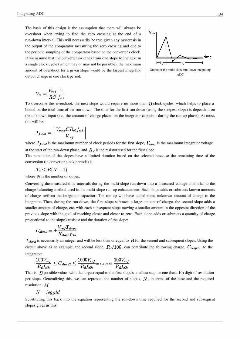
Integrating ADC 134
Output of the multi-slope run-down integratingADC
The basis of this design is the assumption that there will always beovershoot when trying to find the zero crossing at the end of arun-down interval. This will necessarily be true given any hysteresis inthe output of the comparator measuring the zero crossing and due tothe periodic sampling of the comparator based on the converter's clock.If we assume that the converter switches from one slope to the next ina single clock cycle (which may or may not be possible), the maximumamount of overshoot for a given slope would be the largest integratoroutput change in one clock period:
To overcome this overshoot, the next slope would require no more than clock cycles, which helps to place abound on the total time of the run-down. The time for the first-run down (using the steepest slope) is dependent onthe unknown input (i.e., the amount of charge placed on the integrator capacitor during the run-up phase). At most,this will be:
where is the maximum number of clock periods for the first slope, is the maximum integrator voltageat the start of the run-down phase, and is the resistor used for the first slope.The remainder of the slopes have a limited duration based on the selected base, so the remaining time of theconversion (in converter clock periods) is:
where is the number of slopes.Converting the measured time intervals during the multi-slope run-down into a measured voltage is similar to thecharge-balancing method used in the multi-slope run-up enhancement. Each slope adds or subtracts known amountsof charge to/from the integrator capacitor. The run-up will have added some unknown amount of charge to theintegrator. Then, during the run-down, the first slope subtracts a large amount of charge, the second slope adds asmaller amount of charge, etc. with each subsequent slope moving a smaller amount in the opposite direction of theprevious slope with the goal of reaching closer and closer to zero. Each slope adds or subtracts a quantity of chargeproportional to the slope's resistor and the duration of the slope:
is necessarily an integer and will be less than or equal to for the second and subsequent slopes. Using thecircuit above as an example, the second slope, , can contribute the following charge, , to theintegrator:
in steps of
That is, possible values with the largest equal to the first slope's smallest step, or one (base 10) digit of resolutionper slope. Generalizing this, we can represent the number of slopes, , in terms of the base and the requiredresolution, :
Substituting this back into the equation representing the run-down time required for the second and subsequentslopes gives us this:
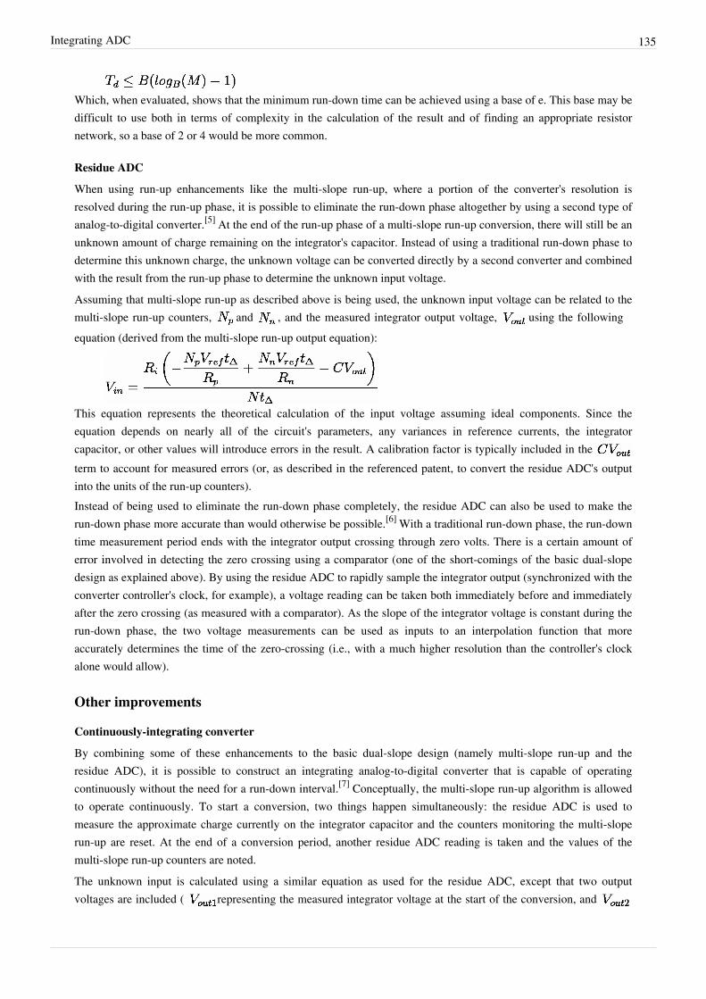
Integrating ADC 135
Which, when evaluated, shows that the minimum run-down time can be achieved using a base of e. This base may bedifficult to use both in terms of complexity in the calculation of the result and of finding an appropriate resistornetwork, so a base of 2 or 4 would be more common.
Residue ADC
When using run-up enhancements like the multi-slope run-up, where a portion of the converter's resolution isresolved during the run-up phase, it is possible to eliminate the run-down phase altogether by using a second type ofanalog-to-digital converter.[5] At the end of the run-up phase of a multi-slope run-up conversion, there will still be anunknown amount of charge remaining on the integrator's capacitor. Instead of using a traditional run-down phase todetermine this unknown charge, the unknown voltage can be converted directly by a second converter and combinedwith the result from the run-up phase to determine the unknown input voltage.Assuming that multi-slope run-up as described above is being used, the unknown input voltage can be related to themulti-slope run-up counters, and , and the measured integrator output voltage, using the followingequation (derived from the multi-slope run-up output equation):
This equation represents the theoretical calculation of the input voltage assuming ideal components. Since theequation depends on nearly all of the circuit's parameters, any variances in reference currents, the integratorcapacitor, or other values will introduce errors in the result. A calibration factor is typically included in the term to account for measured errors (or, as described in the referenced patent, to convert the residue ADC's outputinto the units of the run-up counters).Instead of being used to eliminate the run-down phase completely, the residue ADC can also be used to make therun-down phase more accurate than would otherwise be possible.[6] With a traditional run-down phase, the run-downtime measurement period ends with the integrator output crossing through zero volts. There is a certain amount oferror involved in detecting the zero crossing using a comparator (one of the short-comings of the basic dual-slopedesign as explained above). By using the residue ADC to rapidly sample the integrator output (synchronized with theconverter controller's clock, for example), a voltage reading can be taken both immediately before and immediatelyafter the zero crossing (as measured with a comparator). As the slope of the integrator voltage is constant during therun-down phase, the two voltage measurements can be used as inputs to an interpolation function that moreaccurately determines the time of the zero-crossing (i.e., with a much higher resolution than the controller's clockalone would allow).
Other improvements
Continuously-integrating converter
By combining some of these enhancements to the basic dual-slope design (namely multi-slope run-up and theresidue ADC), it is possible to construct an integrating analog-to-digital converter that is capable of operatingcontinuously without the need for a run-down interval.[7] Conceptually, the multi-slope run-up algorithm is allowedto operate continuously. To start a conversion, two things happen simultaneously: the residue ADC is used tomeasure the approximate charge currently on the integrator capacitor and the counters monitoring the multi-sloperun-up are reset. At the end of a conversion period, another residue ADC reading is taken and the values of themulti-slope run-up counters are noted.The unknown input is calculated using a similar equation as used for the residue ADC, except that two output voltages are included ( representing the measured integrator voltage at the start of the conversion, and

Integrating ADC 136
representing the measured integrator voltage at the end of the conversion.
Such a continuously-integrating converter is very similar to a delta-sigma analog-to-digital converter.
CalibrationIn most variants of the dual-slope integrating converter, the converter's performance is dependent on one or more ofthe circuit parameters. In the case of the basic design, the output of the converter is in terms of the reference voltage.In more advanced designs, there are also dependencies on one or more resistors used in the circuit or on theintegrator capacitor being used. In all cases, even using expensive precision components there may be other effectsthat are not accounted for in the general dual-slope equations (dielectric effect on the capacitor or frequency ortemperature dependencies on any of the components). Any of these variations result in error in the output of theconverter. In the best case, this is simply gain and/or offset error. In the worst case, nonlinearity or nonmonotonicitycould result.Some calibration can be performed internal to the converter (i.e., not requiring any special external input). This typeof calibration would be performed every time the converter is turned on, periodically while the converter is running,or only when a special calibration mode is entered. Another type of calibration requires external inputs of knownquantities (e.g., voltage standards or precision resistance references) and would typically be performed infrequently(every year for equipment used in normal conditions, more often when being used in metrology applications).Of these types of error, offset error is the simplest to correct (assuming that there is a constant offset over the entirerange of the converter). This is often done internal to the converter itself by periodically taking measurements of theground potential. Ideally, measuring the ground should always result in a zero output. Any non-zero output indicatesthe offset error in the converter. That is, if the measurement of ground resulted in an output of 0.001 volts, one canassume that all measurements will be offset by the same amount and can subtract 0.001 from all subsequent results.Gain error can similarly be measured and corrected internally (again assuming that there is a constant gain error overthe entire output range). The voltage reference (or some voltage derived directly from the reference) can be used asthe input to the converter. If the assumption is made that the voltage reference is accurate (to within the tolerances ofthe converter) or that the voltage reference has been externally calibrated against a voltage standard, any error in themeasurement would be a gain error in the converter. If, for example, the measurement of a converter's 5 voltreference resulted in an output of 5.3 volts (after accounting for any offset error), a gain multiplier of 0.94 (5 / 5.3)can be applied to any subsequent measurement results.
Footnotes[1][1] Goeke, HP Journal, page 9[2][2] Hewlett-Packard Catalog, 1981, page 49, stating, "For small inputs, noise becomes a problem and for large inputs, the dielectric absorption of
the capacitor becomes a problem."[3][3] Eng 1994[4][4] Eng 1994, Goeke 1989[5][5] Riedel 1992[6][6] Regier 2001[7][7] Goeke 1992
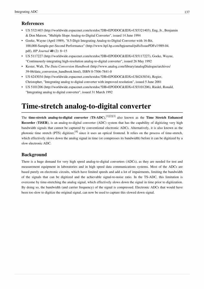
Integrating ADC 137
References• US 5321403 (http:/ / worldwide. espacenet. com/ textdoc?DB=EPODOC& IDX=US5321403), Eng, Jr., Benjamin
& Don Matson, "Multiple Slope Analog-to-Digital Converter", issued 14 June 1994• Goeke, Wayne (April 1989), "8.5-Digit Integrating Analog-to-Digital Converter with 16-Bit,
100,000-Sample-per-Second Performance" (http:/ / www. hpl. hp. com/ hpjournal/ pdfs/ IssuePDFs/ 1989-04.pdf), HP Journal 40 (2): 8–15
• US 5117227 (http:/ / worldwide. espacenet. com/ textdoc?DB=EPODOC& IDX=US5117227), Goeke, Wayne,"Continuously-integrating high-resolution analog-to-digital converter", issued 26 May 1992
• Kester, Walt, The Data Conversion Handbook (http:/ / www. analog. com/ library/ analogDialogue/ archives/39-06/ data_conversion_handbook. html), ISBN 0-7506-7841-0
• US 6243034 (http:/ / worldwide. espacenet. com/ textdoc?DB=EPODOC& IDX=US6243034), Regier,Christopher, "Integrating analog to digital converter with improved resolution", issued 5 June 2001
• US 5101206 (http:/ / worldwide. espacenet. com/ textdoc?DB=EPODOC& IDX=US5101206), Riedel, Ronald,"Integrating analog to digital converter", issued 31 March 1992
Time-stretch analog-to-digital converterThe time-stretch analog-to-digital converter (TS-ADC),[1][2][3] also known as the Time Stretch EnhancedRecorder (TiSER), is an analog-to-digital converter (ADC) system that has the capability of digitizing very highbandwidth signals that cannot be captured by conventional electronic ADCs. Alternatively, it is also known as thephotonic time stretch (PTS) digitizer,[4] since it uses an optical frontend. It relies on the process of time-stretch,which effectively slows down the analog signal in time (or compresses its bandwidth) before it can be digitized by aslow electronic ADC.
BackgroundThere is a huge demand for very high speed analog-to-digital converters (ADCs), as they are needed for test andmeasurement equipment in laboratories and in high speed data communications systems. Most of the ADCs arebased purely on electronic circuits, which have limited speeds and add a lot of impairments, limiting the bandwidthof the signals that can be digitized and the achievable signal-to-noise ratio. In the TS-ADC, this limitation isovercome by time-stretching the analog signal, which effectively slows down the signal in time prior to digitization.By doing so, the bandwidth (and carrier frequency) of the signal is compressed. Electronic ADCs that would havebeen too slow to digitize the original signal, can now be used to capture this slowed down signal.
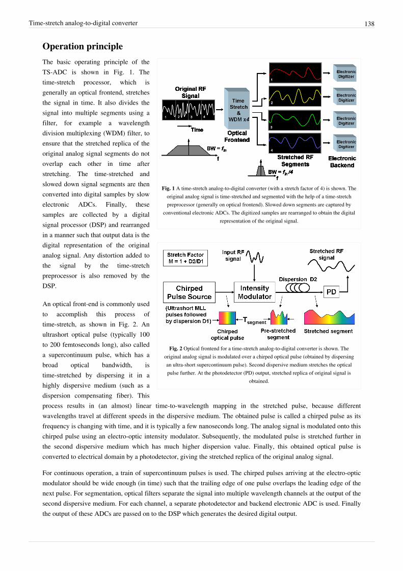
Time-stretch analog-to-digital converter 138
Operation principle
Fig. 1 A time-stretch analog-to-digital converter (with a stretch factor of 4) is shown. Theoriginal analog signal is time-stretched and segmented with the help of a time-stretchpreprocessor (generally on optical frontend). Slowed down segments are captured by
conventional electronic ADCs. The digitized samples are rearranged to obtain the digitalrepresentation of the original signal.
Fig. 2 Optical frontend for a time-stretch analog-to-digital converter is shown. Theoriginal analog signal is modulated over a chirped optical pulse (obtained by dispersingan ultra-short supercontinuum pulse). Second dispersive medium stretches the opticalpulse further. At the photodetector (PD) output, stretched replica of original signal is
obtained.
The basic operating principle of theTS-ADC is shown in Fig. 1. Thetime-stretch processor, which isgenerally an optical frontend, stretchesthe signal in time. It also divides thesignal into multiple segments using afilter, for example a wavelengthdivision multiplexing (WDM) filter, toensure that the stretched replica of theoriginal analog signal segments do notoverlap each other in time afterstretching. The time-stretched andslowed down signal segments are thenconverted into digital samples by slowelectronic ADCs. Finally, thesesamples are collected by a digitalsignal processor (DSP) and rearrangedin a manner such that output data is thedigital representation of the originalanalog signal. Any distortion added tothe signal by the time-stretchpreprocessor is also removed by theDSP.
An optical front-end is commonly usedto accomplish this process oftime-stretch, as shown in Fig. 2. Anultrashort optical pulse (typically 100to 200 femtoseconds long), also calleda supercontinuum pulse, which has abroad optical bandwidth, istime-stretched by dispersing it in ahighly dispersive medium (such as adispersion compensating fiber). Thisprocess results in (an almost) linear time-to-wavelength mapping in the stretched pulse, because differentwavelengths travel at different speeds in the dispersive medium. The obtained pulse is called a chirped pulse as itsfrequency is changing with time, and it is typically a few nanoseconds long. The analog signal is modulated onto thischirped pulse using an electro-optic intensity modulator. Subsequently, the modulated pulse is stretched further inthe second dispersive medium which has much higher dispersion value. Finally, this obtained optical pulse isconverted to electrical domain by a photodetector, giving the stretched replica of the original analog signal.
For continuous operation, a train of supercontinuum pulses is used. The chirped pulses arriving at the electro-opticmodulator should be wide enough (in time) such that the trailing edge of one pulse overlaps the leading edge of thenext pulse. For segmentation, optical filters separate the signal into multiple wavelength channels at the output of thesecond dispersive medium. For each channel, a separate photodetector and backend electronic ADC is used. Finallythe output of these ADCs are passed on to the DSP which generates the desired digital output.

Time-stretch analog-to-digital converter 139
Impulse response of the photonic time-stretch (PTS) systemThe PTS processor is based on specialized analog optical (or microwave photonic) fiber links such as those used incable TV distribution. While the dispersion of fiber is a nuisance in conventional analog optical links, time-stretchtechnique exploits it to slow down the electrical waveform in the optical domain. In the cable TV link, the lightsource is a continuous-wave (CW) laser. In PTS, the source is a chirped pulse laser.
Fig. 4 Capture of a 95-GHz RF tone using the photonic time-stretch digitizer. The signalis captured at an effective sample rate of 10-Terasamples-per-second.
In a conventional analog optical link,dispersion causes the upper and lowermodulation sidebands, foptical ±felectrical, to slip in relative phase. Atcertain frequencies, their beats with theoptical carrier interfere destructively,creating nulls in the frequencyresponse of the system. For practicalsystems the first null is at tens of GHz,which is sufficient for handling mostelectrical signals of interest. Althoughit may seem that the dispersion penaltyplaces a fundamental limit on theimpulse response (or the bandwidth) ofthe time-stretch system, it can beeliminated. The dispersion penaltyvanishes with single-sidebandmodulation. Alternatively, one can use the modulator’s secondary (inverse) output port to eliminate the dispersionpenalty, in much the same way as two antennas can eliminate spatial nulls in wireless communication (hence the twoantennas on top of a WiFi access point). This configuration is termed phase-diversity. For illustration, two calculatedcomplementary transfer functions from a typical phase-diverse time-stretch configuration are plotted in Fig. 4.[5]
Combining the complementary outputs using a maximal ratio combining (MRC) algorithm results in a transferfunction with a flat response in the frequency domain. Thus, the impulse response (bandwidth) of a time-stretchsystem is limited only by the bandwidth of the electro-optic modulator, which is about 120 GHz—a value that isadequate for capturing most electrical waveforms of interest.
Extremely large stretch factors can be obtained using long lengths of fiber, but at the cost of larger loss—a problemthat has been overcome by employing Raman amplification within the dispersive fiber itself, leading to the world’sfastest real-time digitizer,[6] as shown in Fig. 3. Also, using PTS, capture of very high frequency signals with a worldrecord resolution in 10-GHz bandwidth range has been achieved.[7]
Comparison with time lens imagingAnother technique, temporal imaging using a time lens, can also be used to slow down (mostly optical) signals in time. The time-lens concept relies on the mathematical equivalence between spatial diffraction and temporal dispersion, the so-called space-time duality.[8] A lens held at fixed distance from an object produces a magnified visible image. The lens imparts a quadratic phase shift to the spatial frequency components of the optical waves; in conjunction with the free space propagation (object to lens, lens to eye), this generates a magnified image. Owing to the mathematical equivalence between paraxial diffraction and temporal dispersion, an optical waveform can be temporally imaged by a three-step process of dispersing it in time, subjecting it to a phase shift that is quadratic in time (the time lens itself), and dispersing it again. Theoretically, a focused aberration-free image is obtained under a specific condition when the two dispersive elements and the phase shift satisfy the temporal equivalent of the classic

Time-stretch analog-to-digital converter 140
lens equation. Alternatively, the time lens can be used without the second dispersive element to transfer thewaveform’s temporal profile to the spectral domain, analogous to the property that an ordinary lens produces thespatial Fourier transform of an object at its focal points.[9]
In contrast to the time-lens approach, PTS is not based on the space-time duality – there is no lens equation thatneeds to be satisfied to obtain an error-free slowed-down version of the input waveform. Time-stretch technique alsooffers continuous-time acquisition performance, a feature needed for mainstream applications of oscilloscopes.Another important difference between the two techniques is that the time lens requires the input signal to besubjected to high amount of dispersion before further processing. For electrical waveforms, the electronic devicesthat have the required characteristics: (1) high dispersion to loss ratio, (2) uniform dispersion, and (3) broadbandwidths, do not exist. This renders time lens not suitable for slowing down wideband electrical waveforms. Incontrast, PTS does not have such a requirement. It was developed specifically for slowing down electricalwaveforms and enable high speed digitizers.
Application to imaging and spectroscopyIn addition to wideband A/D conversion, photonic time-stretch (PTS) is also an enabling technology forhigh-throughput real-time instrumentation such as imaging [10] and spectroscopy.[11][12] The world's fastest opticalimaging method called serial time-encoded amplified microscopy (STEAM) makes use of the PTS technology toacquire image using a single-pixel photodetector and commercial ADC. Wavelength-time spectroscopy, which alsorelies on photonic time-stretch technique, permits real-time single-shot measurements of rapidly evolving orfluctuating spectra.
References[1] A. S. Bhushan, F. Coppinger, and B. Jalali, “Time-stretched analogue-to-digital conversion," Electronics Letters vol. 34, no. 9, pp. 839–841,
April 1998. (http:/ / ieeexplore. ieee. org/ xpls/ abs_all. jsp?arnumber=682797)[2] A. Fard, S. Gupta, and B. Jalali, "Photonic time-stretch digitizer and its extension to real-time spectroscopy and imaging," Laser & Photonics
Reviews vol. 7, no. 2, pp. 207-263, March 2013. (http:/ / onlinelibrary. wiley. com/ doi/ 10. 1002/ lpor. 201200015/ abstract)[3] Y. Han and B. Jalali, “Photonic Time-Stretched Analog-to-Digital Converter: Fundamental Concepts and Practical Considerations," Journal
of Lightwave Technology, Vol. 21, Issue 12, pp. 3085–3103, Dec. 2003. (http:/ / www. opticsinfobase. org/ abstract. cfm?&uri=JLT-21-12-3085)
[4] J. Capmany and D. Novak, “Microwave photonics combines two worlds," Nature Photonics 1, 319-330 (2007). (http:/ / www. nature. com/nphoton/ journal/ v1/ n6/ abs/ nphoton. 2007. 89. html)
[5] Yan Han, Ozdal Boyraz, Bahram Jalali, "Ultrawide-Band Photonic Time-Stretch A/D Converter Employing Phase Diversity," "IEEETRANSACTIONS ON MICROWAVE THEORY AND TECHNIQUES" VOL. 53, NO. 4, APRIL 2005 (http:/ / ieeexplore. ieee. org/ xpls/abs_all. jsp?arnumber=1420773)
[6] J. Chou, O. Boyraz, D. Solli, and B. Jalali, “Femtosecond real-time single-shot digitizer," Applied Physics Letters 91, 161105 (2007). (http:/ /scitation. aip. org/ getabs/ servlet/ GetabsServlet?prog=normal& id=APPLAB000091000016161105000001& idtype=cvips& gifs=yes)
[7] S. Gupta and B. Jalali, “Time-warp correction and calibration in photonic time-stretch analog-to-digital converter," Optics Letters 33,2674–2676 (2008). (http:/ / www. opticsinfobase. org/ abstract. cfm?uri=ol-33-22-2674)
[8] B. H. Kolner and M. Nazarathy, “Temporal imaging with a time lens," Optics Letters 14, 630-632 (1989) (http:/ / www. opticsinfobase. org/ol/ abstract. cfm?URI=ol-14-12-630)
[9] J. W. Goodman, “Introduction to Fourier Optics," McGraw-Hill (1968).[10] K. Goda, K.K. Tsia, and B. Jalali, "Serial time-encoded amplified imaging for real-time observation of fast dynamic phenomena," Nature
458, 1145–1149, 2009. (http:/ / www. nature. com/ nature/ journal/ v458/ n7242/ full/ nature07980. html)[11] D. R. Solli, J. Chou, and B. Jalali, "Amplified wavelength–time transformation for real-time spectroscopy," Nature Photonics 2, 48-51,
2008. (http:/ / www. nature. com/ nphoton/ journal/ v2/ n1/ full/ nphoton. 2007. 253. html)[12] J. Chou, D. Solli, and B. Jalali, "Real-time spectroscopy with subgigahertz resolution using amplified dispersive Fourier transformation,"
Applied Physics Letters 92, 111102, 2008. (http:/ / apl. aip. org/ resource/ 1/ applab/ v92/ i11/ p111102_s1)

Time-stretch analog-to-digital converter 141
Other resources• G. C. Valley, “Photonic analog-to-digital converters," Opt. Express, vol. 15, no. 5, pp. 1955–1982, March 2007.
(http:/ / www. opticsinfobase. org/ oe/ abstract. cfm?uri=oe-15-5-1955)• Photonic Bandwidth Compression for Instantaneous Wideband A/D Conversion (PHOBIAC) project. (http:/ /
www. darpa. mil/ MTO/ Programs/ phobiac/ index. html)• Short time Fourier transform for time-frequency analysis of ultrawideband signals (http:/ / www. researchgate.
net/ publication/ 3091384_Time-stretched_short-time_Fourier_transform/ )
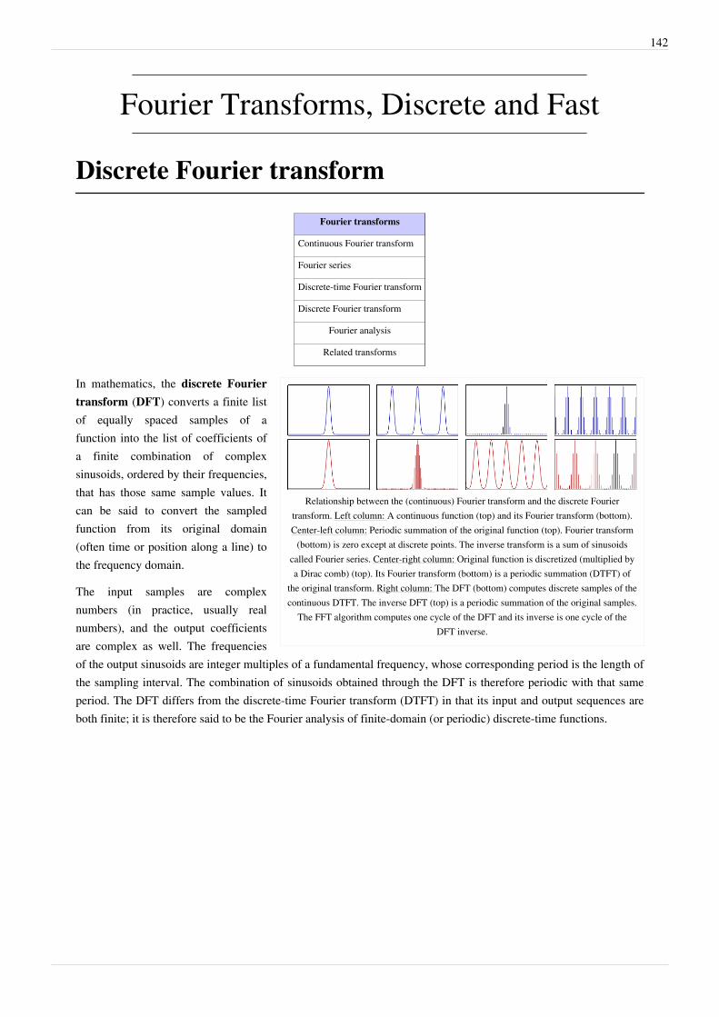
142
Fourier Transforms, Discrete and Fast
Discrete Fourier transform
Fourier transforms
Continuous Fourier transform
Fourier series
Discrete-time Fourier transform
Discrete Fourier transform
Fourier analysis
Related transforms
Relationship between the (continuous) Fourier transform and the discrete Fouriertransform. Left column: A continuous function (top) and its Fourier transform (bottom).Center-left column: Periodic summation of the original function (top). Fourier transform
(bottom) is zero except at discrete points. The inverse transform is a sum of sinusoidscalled Fourier series. Center-right column: Original function is discretized (multiplied bya Dirac comb) (top). Its Fourier transform (bottom) is a periodic summation (DTFT) of
the original transform. Right column: The DFT (bottom) computes discrete samples of thecontinuous DTFT. The inverse DFT (top) is a periodic summation of the original samples.
The FFT algorithm computes one cycle of the DFT and its inverse is one cycle of theDFT inverse.
In mathematics, the discrete Fouriertransform (DFT) converts a finite listof equally spaced samples of afunction into the list of coefficients ofa finite combination of complexsinusoids, ordered by their frequencies,that has those same sample values. Itcan be said to convert the sampledfunction from its original domain(often time or position along a line) tothe frequency domain.
The input samples are complexnumbers (in practice, usually realnumbers), and the output coefficientsare complex as well. The frequenciesof the output sinusoids are integer multiples of a fundamental frequency, whose corresponding period is the length ofthe sampling interval. The combination of sinusoids obtained through the DFT is therefore periodic with that sameperiod. The DFT differs from the discrete-time Fourier transform (DTFT) in that its input and output sequences areboth finite; it is therefore said to be the Fourier analysis of finite-domain (or periodic) discrete-time functions.

Discrete Fourier transform 143
Illustration of using Dirac comb functions and the convolution theorem to model theeffects of sampling and/or periodic summation. At lower left is a DTFT, the spectral
result of sampling s(t) at intervals of T. The spectral sequences at (a) upper right and (b)lower right are respectively computed from (a) one cycle of the periodic summation ofs(t) and (b) one cycle of the periodic summation of the s(nT) sequence. The respective
formulas are (a) the Fourier series integral and (b) the DFT summation. Its similarities tothe original transform, S(f), and its relative computational ease are often the motivation
for computing a DFT sequence.
The DFT is the most important discretetransform, used to perform Fourieranalysis in many practical applications.In digital signal processing, thefunction is any quantity or signal thatvaries over time, such as the pressureof a sound wave, a radio signal, ordaily temperature readings, sampledover a finite time interval (oftendefined by a window function). Inimage processing, the samples can bethe values of pixels along a row orcolumn of a raster image. The DFT isalso used to efficiently solve partialdifferential equations, and to performother operations such as convolutionsor multiplying large integers.
Since it deals with a finite amount ofdata, it can be implemented incomputers by numerical algorithms oreven dedicated hardware. Theseimplementations usually employefficient fast Fourier transform (FFT)algorithms;[1] so much so that theterms "FFT" and "DFT" are often usedinterchangeably. Prior to its current usage, the "FFT" initialism may have also been used for the ambiguous termfinite Fourier transform.
Definition
The sequence of N complex numbers is transformed into an N-periodic sequence of complexnumbers:
(integers) [2] (Eq.1)
Each is a complex number that encodes both amplitude and phase of a sinusoidal component of function .The sinusoid's frequency is k/N cycles per sample. Its amplitude and phase are:
where atan2 is the two-argument form of the arctan function. Due to periodicity (see Periodicity), the customarydomain of k actually computed is [0, N-1]. That is always the case when the DFT is implemented via the FastFourier transform algorithm. But other common domains are [-N/2, N/2-1] (N even) and [-(N-1)/2, (N-1)/2] (Nodd), as when the left and right halves of an FFT output sequence are swapped.
The transform is sometimes denoted by the symbol , as in or or .[3]
Eq.1 can be interpreted or derived in various ways, for example:

Discrete Fourier transform 144
• It completely describes the discrete-time Fourier transform (DTFT) of an N-periodic sequence, which comprisesonly discrete frequency components. (Discrete-time Fourier transform#Periodic data)
• It can also provide uniformly spaced samples of the continuous DTFT of a finite length sequence. (Sampling theDTFT)
• It is the cross correlation of the input sequence, xn, and a complex sinusoid at frequency k/N. Thus it acts like amatched filter for that frequency.
• It is the discrete analogy of the formula for the coefficients of a Fourier series:
(Eq.2)
which is also N-periodic. In the domain this is the inverse transform of Eq.1.The normalization factor multiplying the DFT and IDFT (here 1 and 1/N) and the signs of the exponents are merelyconventions, and differ in some treatments. The only requirements of these conventions are that the DFT and IDFThave opposite-sign exponents and that the product of their normalization factors be 1/N. A normalization of for both the DFT and IDFT, for instance, makes the transforms unitary.In the following discussion the terms "sequence" and "vector" will be considered interchangeable.
Properties
CompletenessThe discrete Fourier transform is an invertible, linear transformation
with denoting the set of complex numbers. In other words, for any N > 0, an N-dimensional complex vector has aDFT and an IDFT which are in turn N-dimensional complex vectors.
Orthogonality
The vectors form an orthogonal basis over the set of N-dimensional
complex vectors:
where is the Kronecker delta. (In the last step, the summation is trivial if , where it is 1+1+⋅⋅⋅=N, andotherwise is a geometric series that can be explicitly summed to obtain zero.) This orthogonality condition can beused to derive the formula for the IDFT from the definition of the DFT, and is equivalent to the unitarity propertybelow.

Discrete Fourier transform 145
The Plancherel theorem and Parseval's theoremIf Xk and Yk are the DFTs of xn and yn respectively then the Plancherel theorem states:
where the star denotes complex conjugation. Parseval's theorem is a special case of the Plancherel theorem andstates:
These theorems are also equivalent to the unitary condition below.
PeriodicityThe periodicity can be shown directly from the definition:
Similarly, it can be shown that the IDFT formula leads to a periodic extension.
Shift theorem
Multiplying by a linear phase for some integer m corresponds to a circular shift of the output :is replaced by , where the subscript is interpreted modulo N (i.e., periodically). Similarly, a circular
shift of the input corresponds to multiplying the output by a linear phase. Mathematically, if represents the vector x then
if
then
and
Circular convolution theorem and cross-correlation theoremThe convolution theorem for the discrete-time Fourier transform indicates that a convolution of two infinitesequences can be obtained as the inverse transform of the product of the individual transforms. An importantsimplification occurs when the sequences are of finite length, N. In terms of the DFT and inverse DFT, it can bewritten as follows:
which is the convolution of the sequence with a sequence extended by periodic summation:
Similarly, the cross-correlation of and is given by:
When either sequence contains a string of zeros, of length L, L+1 of the circular convolution outputs are equivalent to values of Methods have also been developed to use this property as part of an efficient process that constructs with an or sequence potentially much longer than the practical transform size (N). Two
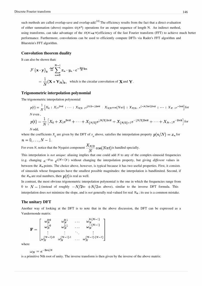
Discrete Fourier transform 146
such methods are called overlap-save and overlap-add.[4] The efficiency results from the fact that a direct evaluationof either summation (above) requires operations for an output sequence of length N. An indirect method,using transforms, can take advantage of the efficiency of the fast Fourier transform (FFT) to achieve much betterperformance. Furthermore, convolutions can be used to efficiently compute DFTs via Rader's FFT algorithm andBluestein's FFT algorithm.
Convolution theorem dualityIt can also be shown that:
which is the circular convolution of and .
Trigonometric interpolation polynomialThe trigonometric interpolation polynomial
for
N even ,
for
N odd,where the coefficients Xk are given by the DFT of xn above, satisfies the interpolation property for
.
For even N, notice that the Nyquist component is handled specially.
This interpolation is not unique: aliasing implies that one could add N to any of the complex-sinusoid frequencies(e.g. changing to ) without changing the interpolation property, but giving different values inbetween the points. The choice above, however, is typical because it has two useful properties. First, it consistsof sinusoids whose frequencies have the smallest possible magnitudes: the interpolation is bandlimited. Second, ifthe are real numbers, then is real as well.In contrast, the most obvious trigonometric interpolation polynomial is the one in which the frequencies range from0 to (instead of roughly to as above), similar to the inverse DFT formula. Thisinterpolation does not minimize the slope, and is not generally real-valued for real ; its use is a common mistake.
The unitary DFTAnother way of looking at the DFT is to note that in the above discussion, the DFT can be expressed as aVandermonde matrix:
where
is a primitive Nth root of unity. The inverse transform is then given by the inverse of the above matrix:
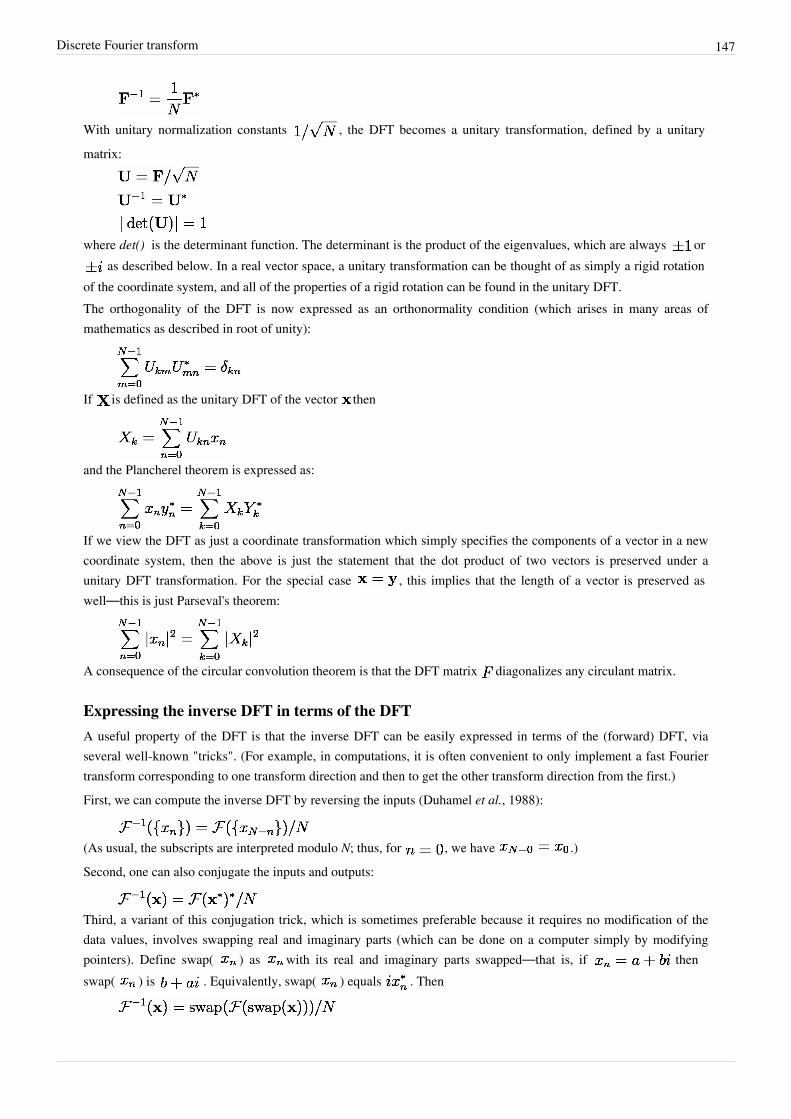
Discrete Fourier transform 147
With unitary normalization constants , the DFT becomes a unitary transformation, defined by a unitarymatrix:
where det() is the determinant function. The determinant is the product of the eigenvalues, which are always oras described below. In a real vector space, a unitary transformation can be thought of as simply a rigid rotation
of the coordinate system, and all of the properties of a rigid rotation can be found in the unitary DFT.The orthogonality of the DFT is now expressed as an orthonormality condition (which arises in many areas ofmathematics as described in root of unity):
If is defined as the unitary DFT of the vector then
and the Plancherel theorem is expressed as:
If we view the DFT as just a coordinate transformation which simply specifies the components of a vector in a newcoordinate system, then the above is just the statement that the dot product of two vectors is preserved under aunitary DFT transformation. For the special case , this implies that the length of a vector is preserved aswell—this is just Parseval's theorem:
A consequence of the circular convolution theorem is that the DFT matrix diagonalizes any circulant matrix.
Expressing the inverse DFT in terms of the DFTA useful property of the DFT is that the inverse DFT can be easily expressed in terms of the (forward) DFT, viaseveral well-known "tricks". (For example, in computations, it is often convenient to only implement a fast Fouriertransform corresponding to one transform direction and then to get the other transform direction from the first.)First, we can compute the inverse DFT by reversing the inputs (Duhamel et al., 1988):
(As usual, the subscripts are interpreted modulo N; thus, for , we have .)Second, one can also conjugate the inputs and outputs:
Third, a variant of this conjugation trick, which is sometimes preferable because it requires no modification of thedata values, involves swapping real and imaginary parts (which can be done on a computer simply by modifyingpointers). Define swap( ) as with its real and imaginary parts swapped—that is, if thenswap( ) is . Equivalently, swap( ) equals . Then
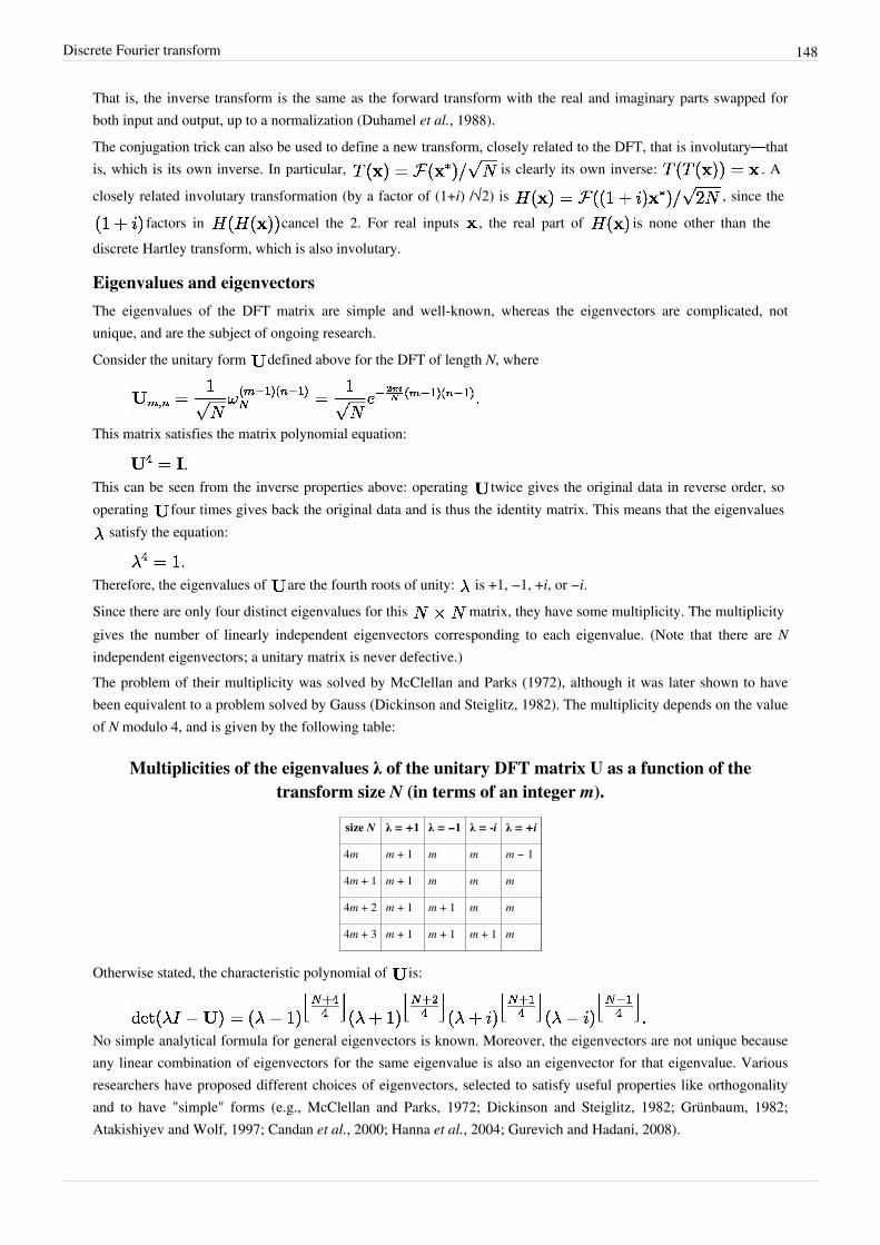
Discrete Fourier transform 148
That is, the inverse transform is the same as the forward transform with the real and imaginary parts swapped forboth input and output, up to a normalization (Duhamel et al., 1988).The conjugation trick can also be used to define a new transform, closely related to the DFT, that is involutary—thatis, which is its own inverse. In particular, is clearly its own inverse: . Aclosely related involutary transformation (by a factor of (1+i) /√2) is , since the
factors in cancel the 2. For real inputs , the real part of is none other than thediscrete Hartley transform, which is also involutary.
Eigenvalues and eigenvectorsThe eigenvalues of the DFT matrix are simple and well-known, whereas the eigenvectors are complicated, notunique, and are the subject of ongoing research.Consider the unitary form defined above for the DFT of length N, where
This matrix satisfies the matrix polynomial equation:
This can be seen from the inverse properties above: operating twice gives the original data in reverse order, sooperating four times gives back the original data and is thus the identity matrix. This means that the eigenvalues
satisfy the equation:
Therefore, the eigenvalues of are the fourth roots of unity: is +1, −1, +i, or −i.Since there are only four distinct eigenvalues for this matrix, they have some multiplicity. The multiplicitygives the number of linearly independent eigenvectors corresponding to each eigenvalue. (Note that there are Nindependent eigenvectors; a unitary matrix is never defective.)The problem of their multiplicity was solved by McClellan and Parks (1972), although it was later shown to havebeen equivalent to a problem solved by Gauss (Dickinson and Steiglitz, 1982). The multiplicity depends on the valueof N modulo 4, and is given by the following table:
Multiplicities of the eigenvalues λ of the unitary DFT matrix U as a function of thetransform size N (in terms of an integer m).
size N λ = +1 λ = −1 λ = -i λ = +i
4m m + 1 m m m − 1
4m + 1 m + 1 m m m
4m + 2 m + 1 m + 1 m m
4m + 3 m + 1 m + 1 m + 1 m
Otherwise stated, the characteristic polynomial of is:
No simple analytical formula for general eigenvectors is known. Moreover, the eigenvectors are not unique becauseany linear combination of eigenvectors for the same eigenvalue is also an eigenvector for that eigenvalue. Variousresearchers have proposed different choices of eigenvectors, selected to satisfy useful properties like orthogonalityand to have "simple" forms (e.g., McClellan and Parks, 1972; Dickinson and Steiglitz, 1982; Grünbaum, 1982;Atakishiyev and Wolf, 1997; Candan et al., 2000; Hanna et al., 2004; Gurevich and Hadani, 2008).
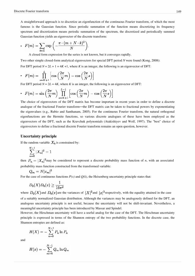
Discrete Fourier transform 149
A straightforward approach is to discretize an eigenfunction of the continuous Fourier transform, of which the mostfamous is the Gaussian function. Since periodic summation of the function means discretizing its frequencyspectrum and discretization means periodic summation of the spectrum, the discretized and periodically summedGaussian function yields an eigenvector of the discrete transform:
• .
A closed form expression for the series is not known, but it converges rapidly.Two other simple closed-form analytical eigenvectors for special DFT period N were found (Kong, 2008):For DFT period N = 2L + 1 = 4K +1, where K is an integer, the following is an eigenvector of DFT:
•
For DFT period N = 2L = 4K, where K is an integer, the following is an eigenvector of DFT:
•
The choice of eigenvectors of the DFT matrix has become important in recent years in order to define a discreteanalogue of the fractional Fourier transform—the DFT matrix can be taken to fractional powers by exponentiatingthe eigenvalues (e.g., Rubio and Santhanam, 2005). For the continuous Fourier transform, the natural orthogonaleigenfunctions are the Hermite functions, so various discrete analogues of these have been employed as theeigenvectors of the DFT, such as the Kravchuk polynomials (Atakishiyev and Wolf, 1997). The "best" choice ofeigenvectors to define a fractional discrete Fourier transform remains an open question, however.
Uncertainty principle
If the random variable is constrained by:
then may be considered to represent a discrete probability mass function of n, with an associatedprobability mass function constructed from the transformed variable:
For the case of continuous functions P(x) and Q(k), the Heisenberg uncertainty principle states that:
where and are the variances of and respectively, with the equality attained in the caseof a suitably normalized Gaussian distribution. Although the variances may be analogously defined for the DFT, ananalogous uncertainty principle is not useful, because the uncertainty will not be shift-invariant. Nevertheless, ameaningful uncertainty principle has been introduced by Massar and Spindel.However, the Hirschman uncertainty will have a useful analog for the case of the DFT. The Hirschman uncertaintyprinciple is expressed in terms of the Shannon entropy of the two probability functions. In the discrete case, theShannon entropies are defined as:
and
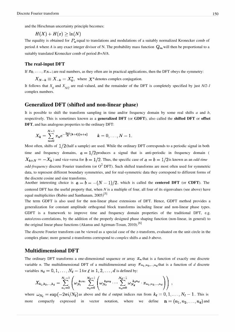
Discrete Fourier transform 150
and the Hirschman uncertainty principle becomes:
The equality is obtained for equal to translations and modulations of a suitably normalized Kronecker comb ofperiod A where A is any exact integer divisor of N. The probability mass function will then be proportional to asuitably translated Kronecker comb of period B=N/A.
The real-input DFTIf are real numbers, as they often are in practical applications, then the DFT obeys the symmetry:
where denotes complex conjugation.It follows that X0 and XN/2 are real-valued, and the remainder of the DFT is completely specified by just N/2-1complex numbers.
Generalized DFT (shifted and non-linear phase)It is possible to shift the transform sampling in time and/or frequency domain by some real shifts a and b,respectively. This is sometimes known as a generalized DFT (or GDFT), also called the shifted DFT or offsetDFT, and has analogous properties to the ordinary DFT:
Most often, shifts of (half a sample) are used. While the ordinary DFT corresponds to a periodic signal in bothtime and frequency domains, produces a signal that is anti-periodic in frequency domain (
) and vice-versa for . Thus, the specific case of is known as an odd-time
odd-frequency discrete Fourier transform (or O2 DFT). Such shifted transforms are most often used for symmetricdata, to represent different boundary symmetries, and for real-symmetric data they correspond to different forms ofthe discrete cosine and sine transforms.Another interesting choice is , which is called the centered DFT (or CDFT). Thecentered DFT has the useful property that, when N is a multiple of four, all four of its eigenvalues (see above) haveequal multiplicities (Rubio and Santhanam, 2005)[5]
The term GDFT is also used for the non-linear phase extensions of DFT. Hence, GDFT method provides ageneralization for constant amplitude orthogonal block transforms including linear and non-linear phase types.GDFT is a framework to improve time and frequency domain properties of the traditional DFT, e.g.auto/cross-correlations, by the addition of the properly designed phase shaping function (non-linear, in general) tothe original linear phase functions (Akansu and Agirman-Tosun, 2010).[6]
The discrete Fourier transform can be viewed as a special case of the z-transform, evaluated on the unit circle in thecomplex plane; more general z-transforms correspond to complex shifts a and b above.
Multidimensional DFTThe ordinary DFT transforms a one-dimensional sequence or array that is a function of exactly one discretevariable n. The multidimensional DFT of a multidimensional array that is a function of d discretevariables for in is defined by:
where as above and the d output indices run from . This is more compactly expressed in vector notation, where we define and
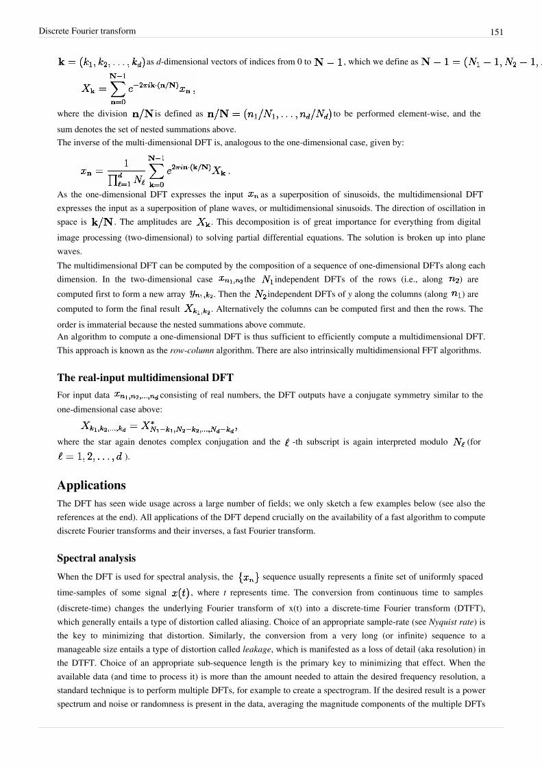
Discrete Fourier transform 151
as d-dimensional vectors of indices from 0 to , which we define as :
where the division is defined as to be performed element-wise, and thesum denotes the set of nested summations above.The inverse of the multi-dimensional DFT is, analogous to the one-dimensional case, given by:
As the one-dimensional DFT expresses the input as a superposition of sinusoids, the multidimensional DFTexpresses the input as a superposition of plane waves, or multidimensional sinusoids. The direction of oscillation inspace is . The amplitudes are . This decomposition is of great importance for everything from digitalimage processing (two-dimensional) to solving partial differential equations. The solution is broken up into planewaves.The multidimensional DFT can be computed by the composition of a sequence of one-dimensional DFTs along eachdimension. In the two-dimensional case the independent DFTs of the rows (i.e., along ) arecomputed first to form a new array . Then the independent DFTs of y along the columns (along ) arecomputed to form the final result . Alternatively the columns can be computed first and then the rows. Theorder is immaterial because the nested summations above commute.An algorithm to compute a one-dimensional DFT is thus sufficient to efficiently compute a multidimensional DFT.This approach is known as the row-column algorithm. There are also intrinsically multidimensional FFT algorithms.
The real-input multidimensional DFTFor input data consisting of real numbers, the DFT outputs have a conjugate symmetry similar to theone-dimensional case above:
where the star again denotes complex conjugation and the -th subscript is again interpreted modulo (for).
ApplicationsThe DFT has seen wide usage across a large number of fields; we only sketch a few examples below (see also thereferences at the end). All applications of the DFT depend crucially on the availability of a fast algorithm to computediscrete Fourier transforms and their inverses, a fast Fourier transform.
Spectral analysis
When the DFT is used for spectral analysis, the sequence usually represents a finite set of uniformly spaced time-samples of some signal , where t represents time. The conversion from continuous time to samples (discrete-time) changes the underlying Fourier transform of x(t) into a discrete-time Fourier transform (DTFT), which generally entails a type of distortion called aliasing. Choice of an appropriate sample-rate (see Nyquist rate) is the key to minimizing that distortion. Similarly, the conversion from a very long (or infinite) sequence to a manageable size entails a type of distortion called leakage, which is manifested as a loss of detail (aka resolution) in the DTFT. Choice of an appropriate sub-sequence length is the primary key to minimizing that effect. When the available data (and time to process it) is more than the amount needed to attain the desired frequency resolution, a standard technique is to perform multiple DFTs, for example to create a spectrogram. If the desired result is a power spectrum and noise or randomness is present in the data, averaging the magnitude components of the multiple DFTs

Discrete Fourier transform 152
is a useful procedure to reduce the variance of the spectrum (also called a periodogram in this context); twoexamples of such techniques are the Welch method and the Bartlett method; the general subject of estimating thepower spectrum of a noisy signal is called spectral estimation.A final source of distortion (or perhaps illusion) is the DFT itself, because it is just a discrete sampling of the DTFT,which is a function of a continuous frequency domain. That can be mitigated by increasing the resolution of theDFT. That procedure is illustrated at Sampling the DTFT.• The procedure is sometimes referred to as zero-padding, which is a particular implementation used in conjunction
with the fast Fourier transform (FFT) algorithm. The inefficiency of performing multiplications and additionswith zero-valued "samples" is more than offset by the inherent efficiency of the FFT.
•• As already noted, leakage imposes a limit on the inherent resolution of the DTFT. So there is a practical limit tothe benefit that can be obtained from a fine-grained DFT.
Filter bankSee FFT filter banks and Sampling the DTFT.
Data compressionThe field of digital signal processing relies heavily on operations in the frequency domain (i.e. on the Fouriertransform). For example, several lossy image and sound compression methods employ the discrete Fouriertransform: the signal is cut into short segments, each is transformed, and then the Fourier coefficients of highfrequencies, which are assumed to be unnoticeable, are discarded. The decompressor computes the inverse transformbased on this reduced number of Fourier coefficients. (Compression applications often use a specialized form of theDFT, the discrete cosine transform or sometimes the modified discrete cosine transform.) Some relatively recentcompression algorithms, however, use wavelet transforms, which give a more uniform compromise between timeand frequency domain than obtained by chopping data into segments and transforming each segment. In the case ofJPEG2000, this avoids the spurious image features that appear when images are highly compressed with the originalJPEG.
Partial differential equationsDiscrete Fourier transforms are often used to solve partial differential equations, where again the DFT is used as anapproximation for the Fourier series (which is recovered in the limit of infinite N). The advantage of this approach isthat it expands the signal in complex exponentials einx, which are eigenfunctions of differentiation: d/dx einx = in einx.Thus, in the Fourier representation, differentiation is simple—we just multiply by i n. (Note, however, that thechoice of n is not unique due to aliasing; for the method to be convergent, a choice similar to that in thetrigonometric interpolation section above should be used.) A linear differential equation with constant coefficients istransformed into an easily solvable algebraic equation. One then uses the inverse DFT to transform the result backinto the ordinary spatial representation. Such an approach is called a spectral method.
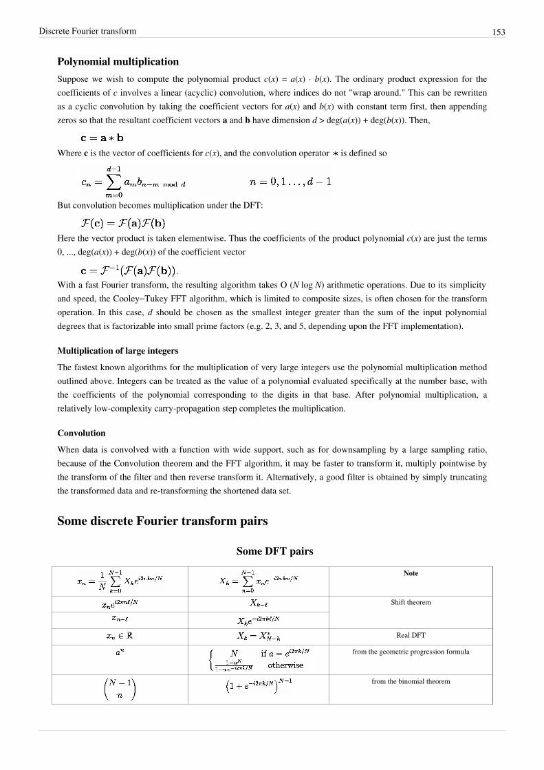
Discrete Fourier transform 153
Polynomial multiplicationSuppose we wish to compute the polynomial product c(x) = a(x) · b(x). The ordinary product expression for thecoefficients of c involves a linear (acyclic) convolution, where indices do not "wrap around." This can be rewrittenas a cyclic convolution by taking the coefficient vectors for a(x) and b(x) with constant term first, then appendingzeros so that the resultant coefficient vectors a and b have dimension d > deg(a(x)) + deg(b(x)). Then,
Where c is the vector of coefficients for c(x), and the convolution operator is defined so
But convolution becomes multiplication under the DFT:
Here the vector product is taken elementwise. Thus the coefficients of the product polynomial c(x) are just the terms0, ..., deg(a(x)) + deg(b(x)) of the coefficient vector
With a fast Fourier transform, the resulting algorithm takes O (N log N) arithmetic operations. Due to its simplicityand speed, the Cooley–Tukey FFT algorithm, which is limited to composite sizes, is often chosen for the transformoperation. In this case, d should be chosen as the smallest integer greater than the sum of the input polynomialdegrees that is factorizable into small prime factors (e.g. 2, 3, and 5, depending upon the FFT implementation).
Multiplication of large integers
The fastest known algorithms for the multiplication of very large integers use the polynomial multiplication methodoutlined above. Integers can be treated as the value of a polynomial evaluated specifically at the number base, withthe coefficients of the polynomial corresponding to the digits in that base. After polynomial multiplication, arelatively low-complexity carry-propagation step completes the multiplication.
Convolution
When data is convolved with a function with wide support, such as for downsampling by a large sampling ratio,because of the Convolution theorem and the FFT algorithm, it may be faster to transform it, multiply pointwise bythe transform of the filter and then reverse transform it. Alternatively, a good filter is obtained by simply truncatingthe transformed data and re-transforming the shortened data set.
Some discrete Fourier transform pairs
Some DFT pairs
Note
Shift theorem
Real DFT
from the geometric progression formula
from the binomial theorem
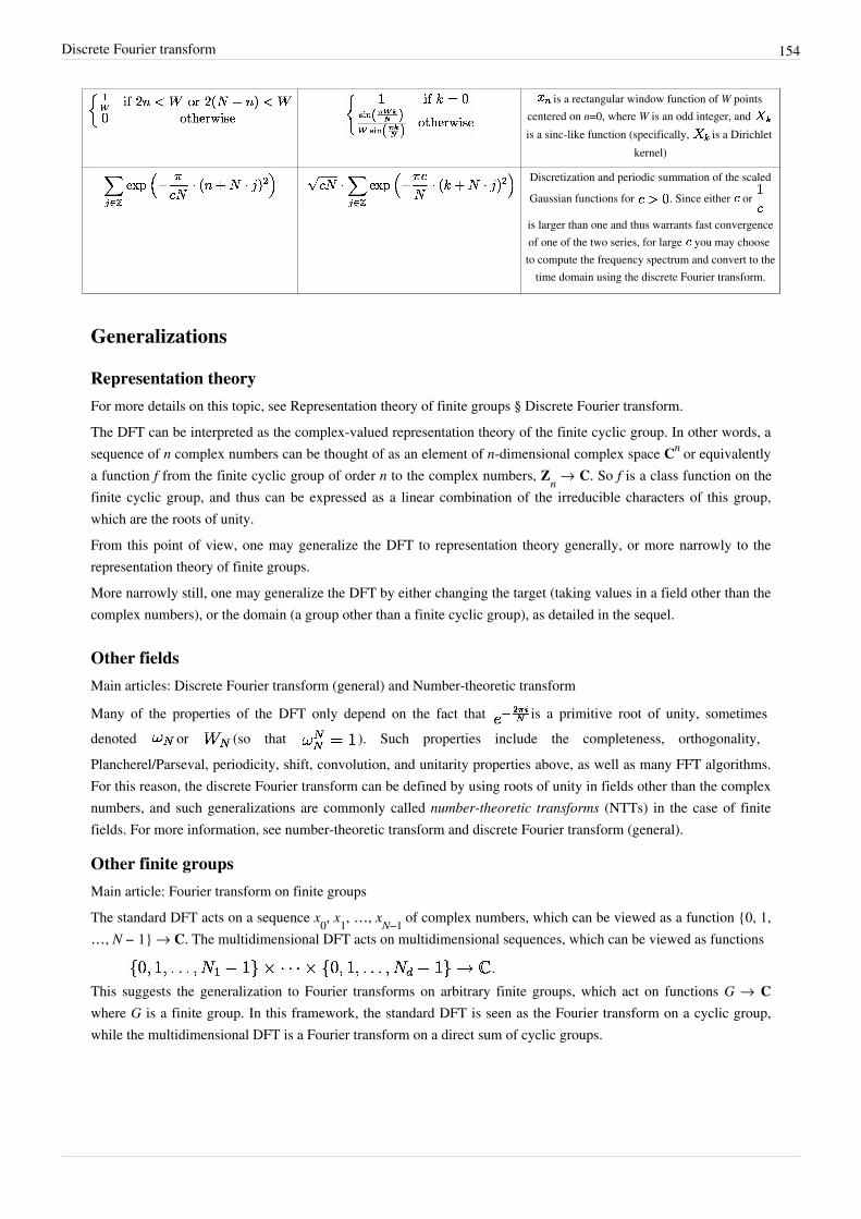
Discrete Fourier transform 154
is a rectangular window function of W pointscentered on n=0, where W is an odd integer, and is a sinc-like function (specifically, is a Dirichlet
kernel)
Discretization and periodic summation of the scaledGaussian functions for . Since either or
is larger than one and thus warrants fast convergenceof one of the two series, for large you may chooseto compute the frequency spectrum and convert to the
time domain using the discrete Fourier transform.
Generalizations
Representation theoryFor more details on this topic, see Representation theory of finite groups § Discrete Fourier transform.The DFT can be interpreted as the complex-valued representation theory of the finite cyclic group. In other words, asequence of n complex numbers can be thought of as an element of n-dimensional complex space Cn or equivalentlya function f from the finite cyclic group of order n to the complex numbers, Zn → C. So f is a class function on thefinite cyclic group, and thus can be expressed as a linear combination of the irreducible characters of this group,which are the roots of unity.From this point of view, one may generalize the DFT to representation theory generally, or more narrowly to therepresentation theory of finite groups.More narrowly still, one may generalize the DFT by either changing the target (taking values in a field other than thecomplex numbers), or the domain (a group other than a finite cyclic group), as detailed in the sequel.
Other fieldsMain articles: Discrete Fourier transform (general) and Number-theoretic transform
Many of the properties of the DFT only depend on the fact that is a primitive root of unity, sometimesdenoted or (so that ). Such properties include the completeness, orthogonality,Plancherel/Parseval, periodicity, shift, convolution, and unitarity properties above, as well as many FFT algorithms.For this reason, the discrete Fourier transform can be defined by using roots of unity in fields other than the complexnumbers, and such generalizations are commonly called number-theoretic transforms (NTTs) in the case of finitefields. For more information, see number-theoretic transform and discrete Fourier transform (general).
Other finite groupsMain article: Fourier transform on finite groupsThe standard DFT acts on a sequence x0, x1, …, xN−1 of complex numbers, which can be viewed as a function {0, 1,…, N − 1} → C. The multidimensional DFT acts on multidimensional sequences, which can be viewed as functions
This suggests the generalization to Fourier transforms on arbitrary finite groups, which act on functions G → Cwhere G is a finite group. In this framework, the standard DFT is seen as the Fourier transform on a cyclic group,while the multidimensional DFT is a Fourier transform on a direct sum of cyclic groups.

Discrete Fourier transform 155
AlternativesMain article: Discrete wavelet transformFor more details on this topic, see Discrete wavelet transform § Comparison with Fourier transform.There are various alternatives to the DFT for various applications, prominent among which are wavelets. The analogof the DFT is the discrete wavelet transform (DWT). From the point of view of time–frequency analysis, a keylimitation of the Fourier transform is that it does not include location information, only frequency information, andthus has difficulty in representing transients. As wavelets have location as well as frequency, they are better able torepresent location, at the expense of greater difficulty representing frequency. For details, see comparison of thediscrete wavelet transform with the discrete Fourier transform.
Notes[1][1] Cooley et al., 1969[2] In this context, it is common to define UNIQ-math-0-fdcc463dc40e329d-QINU to be the Nth primitive root of unity,
UNIQ-math-1-fdcc463dc40e329d-QINU , to obtain the following form:
[3] As a linear transformation on a finite-dimensional vector space, the DFT expression can also be written in terms of a DFT matrix; whenscaled appropriately it becomes a unitary matrix and the Xk can thus be viewed as coefficients of x in an orthonormal basis.
[4] T. G. Stockham, Jr., " High-speed convolution and correlation (http:/ / dl. acm. org/ citation. cfm?id=1464209)," in 1966 Proc. AFIPS SpringJoint Computing Conf. Reprinted in Digital Signal Processing, L. R. Rabiner and C. M. Rader, editors, New York: IEEE Press, 1972.
[5] Santhanam, Balu; Santhanam, Thalanayar S. "Discrete Gauss-Hermite functions and eigenvectors of the centered discrete Fourier transform"(http:/ / thamakau. usc. edu/ Proceedings/ ICASSP 2007/ pdfs/ 0301385. pdf), Proceedings of the 32nd IEEE International Conference onAcoustics, Speech, and Signal Processing (ICASSP 2007, SPTM-P12.4), vol. III, pp. 1385-1388.
[6] Akansu, Ali N.; Agirman-Tosun, Handan "Generalized Discrete Fourier Transform With Nonlinear Phase" (http:/ / web. njit. edu/ ~akansu/PAPERS/ AkansuIEEE-TSP2010. pdf), IEEE Transactions on Signal Processing, vol. 58, no. 9, pp. 4547-4556, Sept. 2010.
Citations
References• Brigham, E. Oran (1988). The fast Fourier transform and its applications. Englewood Cliffs, N.J.: Prentice Hall.
ISBN 0-13-307505-2.• Oppenheim, Alan V.; Schafer, R. W.; and Buck, J. R. (1999). Discrete-time signal processing. Upper Saddle
River, N.J.: Prentice Hall. ISBN 0-13-754920-2.• Smith, Steven W. (1999). "Chapter 8: The Discrete Fourier Transform" (http:/ / www. dspguide. com/ ch8/ 1.
htm). The Scientist and Engineer's Guide to Digital Signal Processing (Second ed.). San Diego, Calif.: CaliforniaTechnical Publishing. ISBN 0-9660176-3-3.
• Cormen, Thomas H.; Charles E. Leiserson, Ronald L. Rivest, and Clifford Stein (2001). "Chapter 30:Polynomials and the FFT". Introduction to Algorithms (Second ed.). MIT Press and McGraw-Hill. pp. 822–848.ISBN 0-262-03293-7. esp. section 30.2: The DFT and FFT, pp. 830–838.
• P. Duhamel, B. Piron, and J. M. Etcheto (1988). "On computing the inverse DFT". IEEE Trans. Acoust., Speechand Sig. Processing 36 (2): 285–286. doi: 10.1109/29.1519 (http:/ / dx. doi. org/ 10. 1109/ 29. 1519).
• J. H. McClellan and T. W. Parks (1972). "Eigenvalues and eigenvectors of the discrete Fourier transformation".IEEE Trans. Audio Electroacoust. 20 (1): 66–74. doi: 10.1109/TAU.1972.1162342 (http:/ / dx. doi. org/ 10. 1109/TAU. 1972. 1162342).
• Bradley W. Dickinson and Kenneth Steiglitz (1982). "Eigenvectors and functions of the discrete Fourier transform". IEEE Trans. Acoust., Speech and Sig. Processing 30 (1): 25–31. doi: 10.1109/TASSP.1982.1163843 (http:/ / dx. doi. org/ 10. 1109/ TASSP. 1982. 1163843). (Note that this paper has an apparent typo in its table of the eigenvalue multiplicities: the +i/−i columns are interchanged. The correct table can be found in McClellan and

Discrete Fourier transform 156
Parks, 1972, and is easily confirmed numerically.)• F. A. Grünbaum (1982). "The eigenvectors of the discrete Fourier transform". J. Math. Anal. Appl. 88 (2):
355–363. doi: 10.1016/0022-247X(82)90199-8 (http:/ / dx. doi. org/ 10. 1016/ 0022-247X(82)90199-8).• Natig M. Atakishiyev and Kurt Bernardo Wolf (1997). "Fractional Fourier-Kravchuk transform". J. Opt. Soc. Am.
A 14 (7): 1467–1477. Bibcode: 1997JOSAA..14.1467A (http:/ / adsabs. harvard. edu/ abs/ 1997JOSAA. . 14.1467A). doi: 10.1364/JOSAA.14.001467 (http:/ / dx. doi. org/ 10. 1364/ JOSAA. 14. 001467).
• C. Candan, M. A. Kutay and H. M.Ozaktas (2000). "The discrete fractional Fourier transform". IEEE Trans. onSignal Processing 48 (5): 1329–1337. Bibcode: 2000ITSP...48.1329C (http:/ / adsabs. harvard. edu/ abs/2000ITSP. . . 48. 1329C). doi: 10.1109/78.839980 (http:/ / dx. doi. org/ 10. 1109/ 78. 839980).
• Magdy Tawfik Hanna, Nabila Philip Attalla Seif, and Waleed Abd El Maguid Ahmed (2004)."Hermite-Gaussian-like eigenvectors of the discrete Fourier transform matrix based on the singular-valuedecomposition of its orthogonal projection matrices". IEEE Trans. Circ. Syst. I 51 (11): 2245–2254. doi:10.1109/TCSI.2004.836850 (http:/ / dx. doi. org/ 10. 1109/ TCSI. 2004. 836850).
• Shamgar Gurevich and Ronny Hadani (2009). "On the diagonalization of the discrete Fourier transform". Appliedand Computational Harmonic Analysis 27 (1): 87–99. arXiv: 0808.3281 (http:/ / arxiv. org/ abs/ 0808. 3281). doi:10.1016/j.acha.2008.11.003 (http:/ / dx. doi. org/ 10. 1016/ j. acha. 2008. 11. 003). preprint at.
• Shamgar Gurevich, Ronny Hadani, and Nir Sochen (2008). "The finite harmonic oscillator and its applications tosequences, communication and radar". IEEE Transactions on Information Theory 54 (9): 4239–4253. arXiv:0808.1495 (http:/ / arxiv. org/ abs/ 0808. 1495). doi: 10.1109/TIT.2008.926440 (http:/ / dx. doi. org/ 10. 1109/TIT. 2008. 926440). preprint at.
• Juan G. Vargas-Rubio and Balu Santhanam (2005). "On the multiangle centered discrete fractional Fouriertransform". IEEE Sig. Proc. Lett. 12 (4): 273–276. Bibcode: 2005ISPL...12..273V (http:/ / adsabs. harvard. edu/abs/ 2005ISPL. . . 12. . 273V). doi: 10.1109/LSP.2005.843762 (http:/ / dx. doi. org/ 10. 1109/ LSP. 2005.843762).
• J. Cooley, P. Lewis, and P. Welch (1969). "The finite Fourier transform". IEEE Trans. Audio Electroacoustics 17(2): 77–85. doi: 10.1109/TAU.1969.1162036 (http:/ / dx. doi. org/ 10. 1109/ TAU. 1969. 1162036).
• F.N. Kong (2008). "Analytic Expressions of Two Discrete Hermite-Gaussian Signals". IEEE Trans. Circuits andSystems –II: Express Briefs. 55 (1): 56–60. doi: 10.1109/TCSII.2007.909865 (http:/ / dx. doi. org/ 10. 1109/TCSII. 2007. 909865).
External links• Matlab tutorial on the Discrete Fourier Transformation (http:/ / www. nbtwiki. net/ doku.
php?id=tutorial:the_discrete_fourier_transformation_dft)• Interactive flash tutorial on the DFT (http:/ / www. fourier-series. com/ fourierseries2/ DFT_tutorial. html)• Mathematics of the Discrete Fourier Transform by Julius O. Smith III (http:/ / ccrma. stanford. edu/ ~jos/ mdft/
mdft. html)• Fast implementation of the DFT - coded in C and under General Public License (GPL) (http:/ / www. fftw. org)• The DFT “à Pied”: Mastering The Fourier Transform in One Day (http:/ / www. dspdimension. com/ admin/
dft-a-pied/ )• Explained: The Discrete Fourier Transform (http:/ / web. mit. edu/ newsoffice/ 2009/ explained-fourier. html)• wavetable Cooker (http:/ / noisemakessound. com/ blofeld-wavetable-cooker/ ) GPL application with graphical
interface written in C, and implementing DFT IDFT to generate a wavetable set
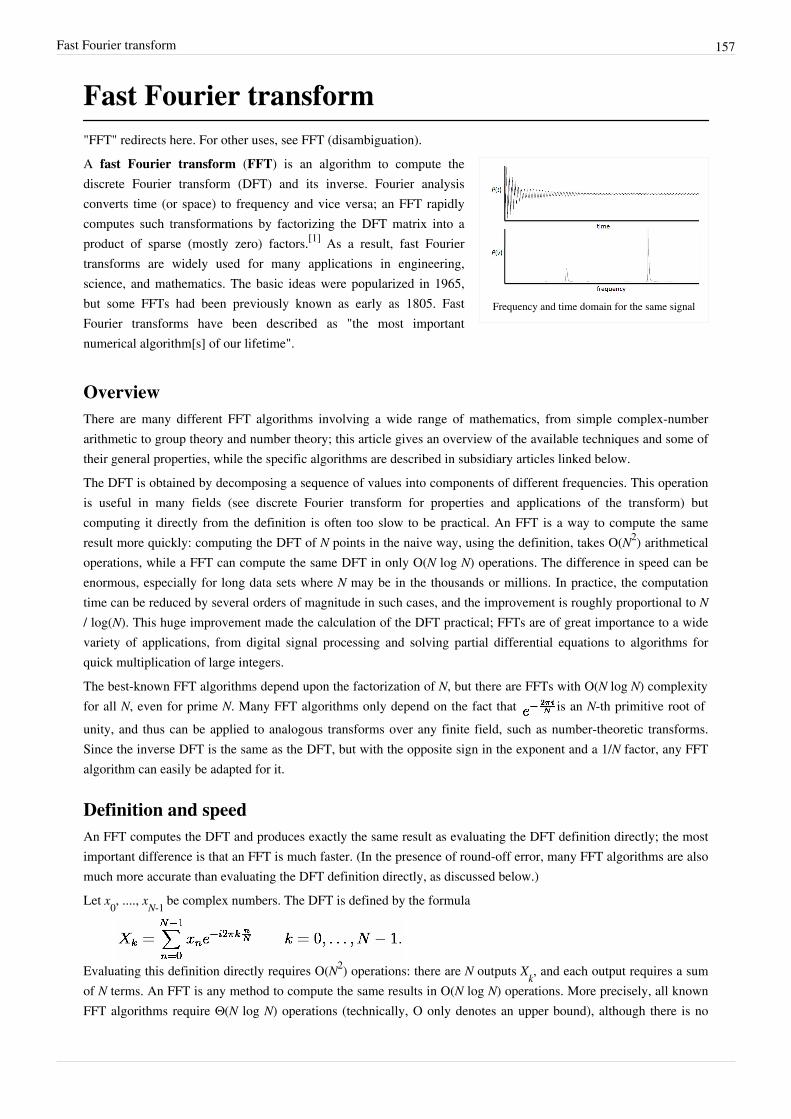
Fast Fourier transform 157
Fast Fourier transform"FFT" redirects here. For other uses, see FFT (disambiguation).
Frequency and time domain for the same signal
A fast Fourier transform (FFT) is an algorithm to compute thediscrete Fourier transform (DFT) and its inverse. Fourier analysisconverts time (or space) to frequency and vice versa; an FFT rapidlycomputes such transformations by factorizing the DFT matrix into aproduct of sparse (mostly zero) factors.[1] As a result, fast Fouriertransforms are widely used for many applications in engineering,science, and mathematics. The basic ideas were popularized in 1965,but some FFTs had been previously known as early as 1805. FastFourier transforms have been described as "the most importantnumerical algorithm[s] of our lifetime".
OverviewThere are many different FFT algorithms involving a wide range of mathematics, from simple complex-numberarithmetic to group theory and number theory; this article gives an overview of the available techniques and some oftheir general properties, while the specific algorithms are described in subsidiary articles linked below.The DFT is obtained by decomposing a sequence of values into components of different frequencies. This operationis useful in many fields (see discrete Fourier transform for properties and applications of the transform) butcomputing it directly from the definition is often too slow to be practical. An FFT is a way to compute the sameresult more quickly: computing the DFT of N points in the naive way, using the definition, takes O(N2) arithmeticaloperations, while a FFT can compute the same DFT in only O(N log N) operations. The difference in speed can beenormous, especially for long data sets where N may be in the thousands or millions. In practice, the computationtime can be reduced by several orders of magnitude in such cases, and the improvement is roughly proportional to N/ log(N). This huge improvement made the calculation of the DFT practical; FFTs are of great importance to a widevariety of applications, from digital signal processing and solving partial differential equations to algorithms forquick multiplication of large integers.The best-known FFT algorithms depend upon the factorization of N, but there are FFTs with O(N log N) complexityfor all N, even for prime N. Many FFT algorithms only depend on the fact that is an N-th primitive root ofunity, and thus can be applied to analogous transforms over any finite field, such as number-theoretic transforms.Since the inverse DFT is the same as the DFT, but with the opposite sign in the exponent and a 1/N factor, any FFTalgorithm can easily be adapted for it.
Definition and speedAn FFT computes the DFT and produces exactly the same result as evaluating the DFT definition directly; the mostimportant difference is that an FFT is much faster. (In the presence of round-off error, many FFT algorithms are alsomuch more accurate than evaluating the DFT definition directly, as discussed below.)Let x0, ...., xN-1 be complex numbers. The DFT is defined by the formula
Evaluating this definition directly requires O(N2) operations: there are N outputs Xk, and each output requires a sum of N terms. An FFT is any method to compute the same results in O(N log N) operations. More precisely, all known FFT algorithms require Θ(N log N) operations (technically, O only denotes an upper bound), although there is no
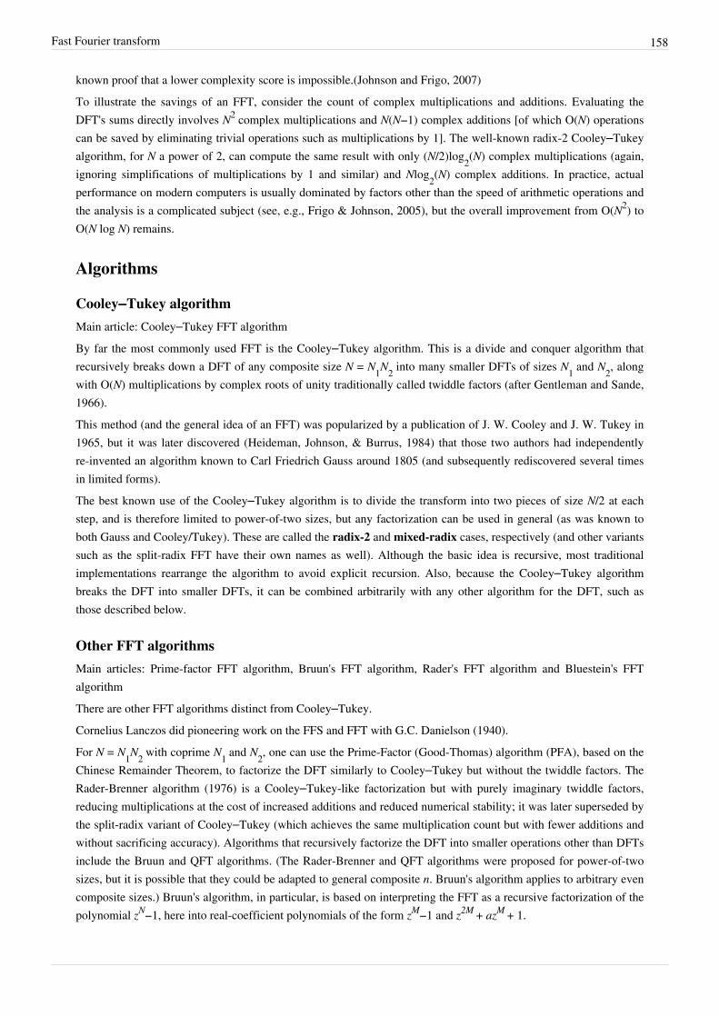
Fast Fourier transform 158
known proof that a lower complexity score is impossible.(Johnson and Frigo, 2007)To illustrate the savings of an FFT, consider the count of complex multiplications and additions. Evaluating theDFT's sums directly involves N2 complex multiplications and N(N−1) complex additions [of which O(N) operationscan be saved by eliminating trivial operations such as multiplications by 1]. The well-known radix-2 Cooley–Tukeyalgorithm, for N a power of 2, can compute the same result with only (N/2)log2(N) complex multiplications (again,ignoring simplifications of multiplications by 1 and similar) and Nlog2(N) complex additions. In practice, actualperformance on modern computers is usually dominated by factors other than the speed of arithmetic operations andthe analysis is a complicated subject (see, e.g., Frigo & Johnson, 2005), but the overall improvement from O(N2) toO(N log N) remains.
Algorithms
Cooley–Tukey algorithmMain article: Cooley–Tukey FFT algorithmBy far the most commonly used FFT is the Cooley–Tukey algorithm. This is a divide and conquer algorithm thatrecursively breaks down a DFT of any composite size N = N1N2 into many smaller DFTs of sizes N1 and N2, alongwith O(N) multiplications by complex roots of unity traditionally called twiddle factors (after Gentleman and Sande,1966).This method (and the general idea of an FFT) was popularized by a publication of J. W. Cooley and J. W. Tukey in1965, but it was later discovered (Heideman, Johnson, & Burrus, 1984) that those two authors had independentlyre-invented an algorithm known to Carl Friedrich Gauss around 1805 (and subsequently rediscovered several timesin limited forms).The best known use of the Cooley–Tukey algorithm is to divide the transform into two pieces of size N/2 at eachstep, and is therefore limited to power-of-two sizes, but any factorization can be used in general (as was known toboth Gauss and Cooley/Tukey). These are called the radix-2 and mixed-radix cases, respectively (and other variantssuch as the split-radix FFT have their own names as well). Although the basic idea is recursive, most traditionalimplementations rearrange the algorithm to avoid explicit recursion. Also, because the Cooley–Tukey algorithmbreaks the DFT into smaller DFTs, it can be combined arbitrarily with any other algorithm for the DFT, such asthose described below.
Other FFT algorithmsMain articles: Prime-factor FFT algorithm, Bruun's FFT algorithm, Rader's FFT algorithm and Bluestein's FFTalgorithmThere are other FFT algorithms distinct from Cooley–Tukey.Cornelius Lanczos did pioneering work on the FFS and FFT with G.C. Danielson (1940).For N = N1N2 with coprime N1 and N2, one can use the Prime-Factor (Good-Thomas) algorithm (PFA), based on theChinese Remainder Theorem, to factorize the DFT similarly to Cooley–Tukey but without the twiddle factors. TheRader-Brenner algorithm (1976) is a Cooley–Tukey-like factorization but with purely imaginary twiddle factors,reducing multiplications at the cost of increased additions and reduced numerical stability; it was later superseded bythe split-radix variant of Cooley–Tukey (which achieves the same multiplication count but with fewer additions andwithout sacrificing accuracy). Algorithms that recursively factorize the DFT into smaller operations other than DFTsinclude the Bruun and QFT algorithms. (The Rader-Brenner and QFT algorithms were proposed for power-of-twosizes, but it is possible that they could be adapted to general composite n. Bruun's algorithm applies to arbitrary evencomposite sizes.) Bruun's algorithm, in particular, is based on interpreting the FFT as a recursive factorization of thepolynomial zN−1, here into real-coefficient polynomials of the form zM−1 and z2M + azM + 1.

Fast Fourier transform 159
Another polynomial viewpoint is exploited by the Winograd algorithm, which factorizes zN−1 into cyclotomicpolynomials—these often have coefficients of 1, 0, or −1, and therefore require few (if any) multiplications, soWinograd can be used to obtain minimal-multiplication FFTs and is often used to find efficient algorithms for smallfactors. Indeed, Winograd showed that the DFT can be computed with only O(N) irrational multiplications, leadingto a proven achievable lower bound on the number of multiplications for power-of-two sizes; unfortunately, thiscomes at the cost of many more additions, a tradeoff no longer favorable on modern processors with hardwaremultipliers. In particular, Winograd also makes use of the PFA as well as an algorithm by Rader for FFTs of primesizes.Rader's algorithm, exploiting the existence of a generator for the multiplicative group modulo prime N, expresses aDFT of prime size n as a cyclic convolution of (composite) size N−1, which can then be computed by a pair ofordinary FFTs via the convolution theorem (although Winograd uses other convolution methods). Anotherprime-size FFT is due to L. I. Bluestein, and is sometimes called the chirp-z algorithm; it also re-expresses a DFT asa convolution, but this time of the same size (which can be zero-padded to a power of two and evaluated by radix-2Cooley–Tukey FFTs, for example), via the identity .
FFT algorithms specialized for real and/or symmetric dataIn many applications, the input data for the DFT are purely real, in which case the outputs satisfy the symmetry
and efficient FFT algorithms have been designed for this situation (see e.g. Sorensen, 1987). One approach consistsof taking an ordinary algorithm (e.g. Cooley–Tukey) and removing the redundant parts of the computation, savingroughly a factor of two in time and memory. Alternatively, it is possible to express an even-length real-input DFT asa complex DFT of half the length (whose real and imaginary parts are the even/odd elements of the original realdata), followed by O(N) post-processing operations.It was once believed that real-input DFTs could be more efficiently computed by means of the discrete Hartleytransform (DHT), but it was subsequently argued that a specialized real-input DFT algorithm (FFT) can typically befound that requires fewer operations than the corresponding DHT algorithm (FHT) for the same number of inputs.Bruun's algorithm (above) is another method that was initially proposed to take advantage of real inputs, but it hasnot proved popular.There are further FFT specializations for the cases of real data that have even/odd symmetry, in which case one cangain another factor of (roughly) two in time and memory and the DFT becomes the discrete cosine/sine transform(s)(DCT/DST). Instead of directly modifying an FFT algorithm for these cases, DCTs/DSTs can also be computed viaFFTs of real data combined with O(N) pre/post processing.
Computational issues
Bounds on complexity and operation counts
List of unsolved problems in computer science
What is the lower bound on the complexity of fast Fourier transform algorithms? Can they be faster than Θ(N log N)?
A fundamental question of longstanding theoretical interest is to prove lower bounds on the complexity and exactoperation counts of fast Fourier transforms, and many open problems remain. It is not even rigorously provedwhether DFTs truly require Ω(N log(N)) (i.e., order N log(N) or greater) operations, even for the simple case ofpower of two sizes, although no algorithms with lower complexity are known. In particular, the count of arithmeticoperations is usually the focus of such questions, although actual performance on modern-day computers isdetermined by many other factors such as cache or CPU pipeline optimization.
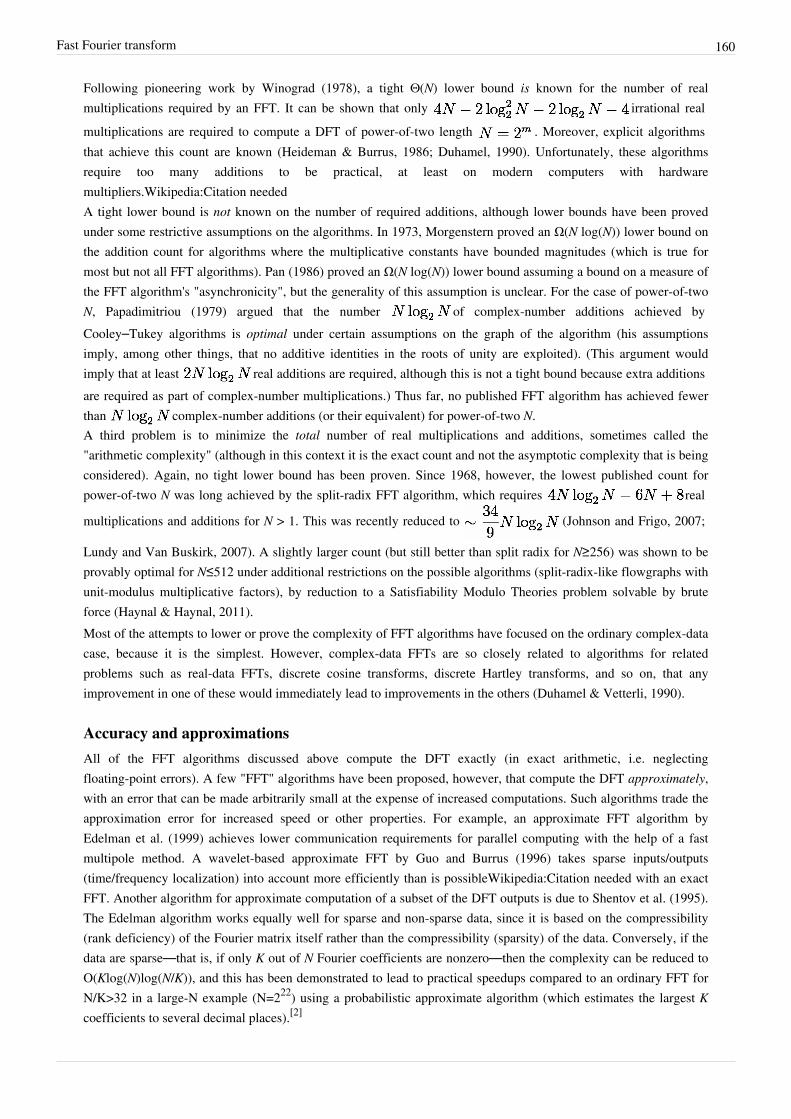
Fast Fourier transform 160
Following pioneering work by Winograd (1978), a tight Θ(N) lower bound is known for the number of realmultiplications required by an FFT. It can be shown that only irrational realmultiplications are required to compute a DFT of power-of-two length . Moreover, explicit algorithmsthat achieve this count are known (Heideman & Burrus, 1986; Duhamel, 1990). Unfortunately, these algorithmsrequire too many additions to be practical, at least on modern computers with hardwaremultipliers.Wikipedia:Citation neededA tight lower bound is not known on the number of required additions, although lower bounds have been provedunder some restrictive assumptions on the algorithms. In 1973, Morgenstern proved an Ω(N log(N)) lower bound onthe addition count for algorithms where the multiplicative constants have bounded magnitudes (which is true formost but not all FFT algorithms). Pan (1986) proved an Ω(N log(N)) lower bound assuming a bound on a measure ofthe FFT algorithm's "asynchronicity", but the generality of this assumption is unclear. For the case of power-of-twoN, Papadimitriou (1979) argued that the number of complex-number additions achieved byCooley–Tukey algorithms is optimal under certain assumptions on the graph of the algorithm (his assumptionsimply, among other things, that no additive identities in the roots of unity are exploited). (This argument wouldimply that at least real additions are required, although this is not a tight bound because extra additionsare required as part of complex-number multiplications.) Thus far, no published FFT algorithm has achieved fewerthan complex-number additions (or their equivalent) for power-of-two N.A third problem is to minimize the total number of real multiplications and additions, sometimes called the"arithmetic complexity" (although in this context it is the exact count and not the asymptotic complexity that is beingconsidered). Again, no tight lower bound has been proven. Since 1968, however, the lowest published count forpower-of-two N was long achieved by the split-radix FFT algorithm, which requires real
multiplications and additions for N > 1. This was recently reduced to (Johnson and Frigo, 2007;
Lundy and Van Buskirk, 2007). A slightly larger count (but still better than split radix for N≥256) was shown to beprovably optimal for N≤512 under additional restrictions on the possible algorithms (split-radix-like flowgraphs withunit-modulus multiplicative factors), by reduction to a Satisfiability Modulo Theories problem solvable by bruteforce (Haynal & Haynal, 2011).Most of the attempts to lower or prove the complexity of FFT algorithms have focused on the ordinary complex-datacase, because it is the simplest. However, complex-data FFTs are so closely related to algorithms for relatedproblems such as real-data FFTs, discrete cosine transforms, discrete Hartley transforms, and so on, that anyimprovement in one of these would immediately lead to improvements in the others (Duhamel & Vetterli, 1990).
Accuracy and approximationsAll of the FFT algorithms discussed above compute the DFT exactly (in exact arithmetic, i.e. neglectingfloating-point errors). A few "FFT" algorithms have been proposed, however, that compute the DFT approximately,with an error that can be made arbitrarily small at the expense of increased computations. Such algorithms trade theapproximation error for increased speed or other properties. For example, an approximate FFT algorithm byEdelman et al. (1999) achieves lower communication requirements for parallel computing with the help of a fastmultipole method. A wavelet-based approximate FFT by Guo and Burrus (1996) takes sparse inputs/outputs(time/frequency localization) into account more efficiently than is possibleWikipedia:Citation needed with an exactFFT. Another algorithm for approximate computation of a subset of the DFT outputs is due to Shentov et al. (1995).The Edelman algorithm works equally well for sparse and non-sparse data, since it is based on the compressibility(rank deficiency) of the Fourier matrix itself rather than the compressibility (sparsity) of the data. Conversely, if thedata are sparse—that is, if only K out of N Fourier coefficients are nonzero—then the complexity can be reduced toO(Klog(N)log(N/K)), and this has been demonstrated to lead to practical speedups compared to an ordinary FFT forN/K>32 in a large-N example (N=222) using a probabilistic approximate algorithm (which estimates the largest Kcoefficients to several decimal places).[2]

Fast Fourier transform 161
Even the "exact" FFT algorithms have errors when finite-precision floating-point arithmetic is used, but these errorsare typically quite small; most FFT algorithms, e.g. Cooley–Tukey, have excellent numerical properties as aconsequence of the pairwise summation structure of the algorithms. The upper bound on the relative error for theCooley–Tukey algorithm is O(ε log N), compared to O(εN3/2) for the naïve DFT formula (Gentleman and Sande,1966), where ε is the machine floating-point relative precision. In fact, the root mean square (rms) errors are muchbetter than these upper bounds, being only O(ε √log N) for Cooley–Tukey and O(ε √N) for the naïve DFT(Schatzman, 1996). These results, however, are very sensitive to the accuracy of the twiddle factors used in the FFT(i.e. the trigonometric function values), and it is not unusual for incautious FFT implementations to have much worseaccuracy, e.g. if they use inaccurate trigonometric recurrence formulas. Some FFTs other than Cooley–Tukey, suchas the Rader-Brenner algorithm, are intrinsically less stable.In fixed-point arithmetic, the finite-precision errors accumulated by FFT algorithms are worse, with rms errorsgrowing as O(√N) for the Cooley–Tukey algorithm (Welch, 1969). Moreover, even achieving this accuracy requirescareful attention to scaling in order to minimize the loss of precision, and fixed-point FFT algorithms involverescaling at each intermediate stage of decompositions like Cooley–Tukey.To verify the correctness of an FFT implementation, rigorous guarantees can be obtained in O(Nlog(N)) time by asimple procedure checking the linearity, impulse-response, and time-shift properties of the transform on randominputs (Ergün, 1995).
Multidimensional FFTsAs defined in the multidimensional DFT article, the multidimensional DFT
transforms an array xn
with a d-dimensional vector of indices by a set of d nested summations(over for each j), where the division n/N, defined as , isperformed element-wise. Equivalently, it is the composition of a sequence of d sets of one-dimensional DFTs,performed along one dimension at a time (in any order).This compositional viewpoint immediately provides the simplest and most common multidimensional DFTalgorithm, known as the row-column algorithm (after the two-dimensional case, below). That is, one simplyperforms a sequence of d one-dimensional FFTs (by any of the above algorithms): first you transform along the n1dimension, then along the n2 dimension, and so on (or actually, any ordering will work). This method is easily shownto have the usual O(Nlog(N)) complexity, where is the total number of data pointstransformed. In particular, there are N/N1 transforms of size N1, etcetera, so the complexity of the sequence of FFTsis:
In two dimensions, the xk
can be viewed as an matrix, and this algorithm corresponds to first performingthe FFT of all the rows (resp. columns), grouping the resulting transformed rows (resp. columns) together as another
matrix, and then performing the FFT on each of the columns (resp. rows) of this second matrix, andsimilarly grouping the results into the final result matrix.In more than two dimensions, it is often advantageous for cache locality to group the dimensions recursively. For example, a three-dimensional FFT might first perform two-dimensional FFTs of each planar "slice" for each fixed n1, and then perform the one-dimensional FFTs along the n1 direction. More generally, an asymptotically optimal cache-oblivious algorithm consists of recursively dividing the dimensions into two groups and

Fast Fourier transform 162
that are transformed recursively (rounding if d is not even) (see Frigo and Johnson, 2005). Still, this remains astraightforward variation of the row-column algorithm that ultimately requires only a one-dimensional FFTalgorithm as the base case, and still has O(Nlog(N)) complexity. Yet another variation is to perform matrixtranspositions in between transforming subsequent dimensions, so that the transforms operate on contiguous data;this is especially important for out-of-core and distributed memory situations where accessing non-contiguous data isextremely time-consuming.There are other multidimensional FFT algorithms that are distinct from the row-column algorithm, although all ofthem have O(Nlog(N)) complexity. Perhaps the simplest non-row-column FFT is the vector-radix FFT algorithm,which is a generalization of the ordinary Cooley–Tukey algorithm where one divides the transform dimensions by avector of radices at each step. (This may also have cache benefits.) The simplest case ofvector-radix is where all of the radices are equal (e.g. vector-radix-2 divides all of the dimensions by two), but this isnot necessary. Vector radix with only a single non-unit radix at a time, i.e. , isessentially a row-column algorithm. Other, more complicated, methods include polynomial transform algorithms dueto Nussbaumer (1977), which view the transform in terms of convolutions and polynomial products. See Duhameland Vetterli (1990) for more information and references.
Other generalizationsAn O(N5/2log(N)) generalization to spherical harmonics on the sphere S2 with N2 nodes was described byMohlenkamp (1999), along with an algorithm conjectured (but not proven) to have O(N2 log2(N)) complexity;Mohlenkamp also provides an implementation in the libftsh library [3]. A spherical-harmonic algorithm withO(N2log(N)) complexity is described by Rokhlin and Tygert (2006).The Fast Folding Algorithm is analogous to the FFT, except that it operates on a series of binned waveforms ratherthan a series of real or complex scalar values. Rotation (which in the FFT is multiplication by a complex phasor) is acircular shift of the component waveform.Various groups have also published "FFT" algorithms for non-equispaced data, as reviewed in Potts et al. (2001).Such algorithms do not strictly compute the DFT (which is only defined for equispaced data), but rather someapproximation thereof (a non-uniform discrete Fourier transform, or NDFT, which itself is often computed onlyapproximately). More generally there are various other methods of spectral estimation.
References[1] Charles Van Loan, Computational Frameworks for the Fast Fourier Transform (SIAM, 1992).[2] Haitham Hassanieh, Piotr Indyk, Dina Katabi, and Eric Price, "Simple and Practical Algorithm for Sparse Fourier Transform" (http:/ / www.
mit. edu/ ~ecprice/ papers/ sparse-fft-soda. pdf) (PDF), ACM-SIAM Symposium On Discrete Algorithms (SODA), Kyoto, January 2012. Seealso the sFFT Web Page (http:/ / groups. csail. mit. edu/ netmit/ sFFT/ ).
[3] http:/ / www. math. ohiou. edu/ ~mjm/ research/ libftsh. html
• Brenner, N.; Rader, C. (1976). "A New Principle for Fast Fourier Transformation". IEEE Acoustics, Speech &Signal Processing 24 (3): 264–266. doi: 10.1109/TASSP.1976.1162805 (http:/ / dx. doi. org/ 10. 1109/ TASSP.1976. 1162805).
• Brigham, E. O. (2002). The Fast Fourier Transform. New York: Prentice-Hall• Thomas H. Cormen, Charles E. Leiserson, Ronald L. Rivest, and Clifford Stein, 2001. Introduction to Algorithms,
2nd. ed. MIT Press and McGraw-Hill. ISBN 0-262-03293-7. Especially chapter 30, "Polynomials and the FFT."• Duhamel, Pierre (1990). "Algorithms meeting the lower bounds on the multiplicative complexity of length-
DFTs and their connection with practical algorithms". IEEE Trans. Acoust. Speech. Sig. Proc. 38 (9): 1504–151.doi: 10.1109/29.60070 (http:/ / dx. doi. org/ 10. 1109/ 29. 60070).
• P. Duhamel and M. Vetterli, 1990, Fast Fourier transforms: a tutorial review and a state of the art (http:/ / dx. doi.org/ 10. 1016/ 0165-1684(90)90158-U), Signal Processing 19: 259–299.
Fast Fourier transform 163
• A. Edelman, P. McCorquodale, and S. Toledo, 1999, The Future Fast Fourier Transform? (http:/ / dx. doi. org/ 10.1137/ S1064827597316266), SIAM J. Sci. Computing 20: 1094–1114.
• D. F. Elliott, & K. R. Rao, 1982, Fast transforms: Algorithms, analyses, applications. New York: AcademicPress.
• Funda Ergün, 1995, Testing multivariate linear functions: Overcoming the generator bottleneck (http:/ / dx. doi.org/ 10. 1145/ 225058. 225167), Proc. 27th ACM Symposium on the Theory of Computing: 407–416.
• M. Frigo and S. G. Johnson, 2005, " The Design and Implementation of FFTW3 (http:/ / fftw. org/fftw-paper-ieee. pdf)," Proceedings of the IEEE 93: 216–231.
• Carl Friedrich Gauss, 1866. " Theoria interpolationis methodo nova tractata (http:/ / lseet. univ-tln. fr/ ~iaroslav/Gauss_Theoria_interpolationis_methodo_nova_tractata. php)," Werke band 3, 265–327. Göttingen: KöniglicheGesellschaft der Wissenschaften.
• W. M. Gentleman and G. Sande, 1966, "Fast Fourier transforms—for fun and profit," Proc. AFIPS 29: 563–578.doi: 10.1145/1464291.1464352 (http:/ / dx. doi. org/ 10. 1145/ 1464291. 1464352)
• H. Guo and C. S. Burrus, 1996, Fast approximate Fourier transform via wavelets transform (http:/ / dx. doi. org/10. 1117/ 12. 255236), Proc. SPIE Intl. Soc. Opt. Eng. 2825: 250–259.
• H. Guo, G. A. Sitton, C. S. Burrus, 1994, The Quick Discrete Fourier Transform (http:/ / dx. doi. org/ 10. 1109/ICASSP. 1994. 389994), Proc. IEEE Conf. Acoust. Speech and Sig. Processing (ICASSP) 3: 445–448.
• Steve Haynal and Heidi Haynal, " Generating and Searching Families of FFT Algorithms (http:/ / jsat. ewi.tudelft. nl/ content/ volume7/ JSAT7_13_Haynal. pdf)", Journal on Satisfiability, Boolean Modeling andComputation vol. 7, pp. 145–187 (2011).
• Heideman, M. T.; Johnson, D. H.; Burrus, C. S. (1984). "Gauss and the history of the fast Fourier transform".IEEE ASSP Magazine 1 (4): 14–21. doi: 10.1109/MASSP.1984.1162257 (http:/ / dx. doi. org/ 10. 1109/ MASSP.1984. 1162257).
• Heideman, Michael T.; Burrus, C. Sidney (1986). "On the number of multiplications necessary to compute alength- DFT". IEEE Trans. Acoust. Speech. Sig. Proc. 34 (1): 91–95. doi: 10.1109/TASSP.1986.1164785(http:/ / dx. doi. org/ 10. 1109/ TASSP. 1986. 1164785).
• S. G. Johnson and M. Frigo, 2007. " A modified split-radix FFT with fewer arithmetic operations (http:/ / www.fftw. org/ newsplit. pdf)," IEEE Trans. Signal Processing 55 (1): 111–119.
• T. Lundy and J. Van Buskirk, 2007. "A new matrix approach to real FFTs and convolutions of length 2k,"Computing 80 (1): 23-45.
• Kent, Ray D. and Read, Charles (2002). Acoustic Analysis of Speech. ISBN 0-7693-0112-6. Cites Strang, G.(1994)/May–June). Wavelets. American Scientist, 82, 250-255.
• Morgenstern, Jacques (1973). "Note on a lower bound of the linear complexity of the fast Fourier transform". J.ACM 20 (2): 305–306. doi: 10.1145/321752.321761 (http:/ / dx. doi. org/ 10. 1145/ 321752. 321761).
• Mohlenkamp, M. J. (1999). "A fast transform for spherical harmonics" (http:/ / www. math. ohiou. edu/ ~mjm/research/ MOHLEN1999P. pdf). J. Fourier Anal. Appl. 5 (2-3): 159–184. doi: 10.1007/BF01261607 (http:/ / dx.doi. org/ 10. 1007/ BF01261607).
• Nussbaumer, H. J. (1977). "Digital filtering using polynomial transforms". Electronics Lett. 13 (13): 386–387.doi: 10.1049/el:19770280 (http:/ / dx. doi. org/ 10. 1049/ el:19770280).
• V. Pan, 1986, The trade-off between the additive complexity and the asyncronicity of linear and bilinearalgorithms (http:/ / dx. doi. org/ 10. 1016/ 0020-0190(86)90035-9), Information Proc. Lett. 22: 11-14.
• Christos H. Papadimitriou, 1979, Optimality of the fast Fourier transform (http:/ / dx. doi. org/ 10. 1145/ 322108.322118), J. ACM 26: 95-102.
• D. Potts, G. Steidl, and M. Tasche, 2001. " Fast Fourier transforms for nonequispaced data: A tutorial (http:/ /www. tu-chemnitz. de/ ~potts/ paper/ ndft. pdf)", in: J.J. Benedetto and P. Ferreira (Eds.), Modern SamplingTheory: Mathematics and Applications (Birkhauser).
Fast Fourier transform 164
• Press, WH; Teukolsky, SA; Vetterling, WT; Flannery, BP (2007), "Chapter 12. Fast Fourier Transform" (http:/ /apps. nrbook. com/ empanel/ index. html#pg=600), Numerical Recipes: The Art of Scientific Computing (3rd ed.),New York: Cambridge University Press, ISBN 978-0-521-88068-8
• Rokhlin, Vladimir; Tygert, Mark (2006). "Fast algorithms for spherical harmonic expansions". SIAM J. Sci.Computing 27 (6): 1903–1928. doi: 10.1137/050623073 (http:/ / dx. doi. org/ 10. 1137/ 050623073).
• James C. Schatzman, 1996, Accuracy of the discrete Fourier transform and the fast Fourier transform (http:/ /portal. acm. org/ citation. cfm?id=240432), SIAM J. Sci. Comput. 17: 1150–1166.
• Shentov, O. V.; Mitra, S. K.; Heute, U.; Hossen, A. N. (1995). "Subband DFT. I. Definition, interpretations andextensions". Signal Processing 41 (3): 261–277. doi: 10.1016/0165-1684(94)00103-7 (http:/ / dx. doi. org/ 10.1016/ 0165-1684(94)00103-7).
• Sorensen, H. V.; Jones, D. L.; Heideman, M. T.; Burrus, C. S. (1987). "Real-valued fast Fourier transformalgorithms". IEEE Trans. Acoust. Speech Sig. Processing 35 (35): 849–863. doi: 10.1109/TASSP.1987.1165220(http:/ / dx. doi. org/ 10. 1109/ TASSP. 1987. 1165220). See also Sorensen, H.; Jones, D.; Heideman, M.; Burrus,C. (1987). "Corrections to "Real-valued fast Fourier transform algorithms"". IEEE Transactions on Acoustics,Speech, and Signal Processing 35 (9): 1353–1353. doi: 10.1109/TASSP.1987.1165284 (http:/ / dx. doi. org/ 10.1109/ TASSP. 1987. 1165284).
• Welch, Peter D. (1969). "A fixed-point fast Fourier transform error analysis". IEEE Trans. Audio Electroacoustics17 (2): 151–157. doi: 10.1109/TAU.1969.1162035 (http:/ / dx. doi. org/ 10. 1109/ TAU. 1969. 1162035).
• Winograd, S. (1978). "On computing the discrete Fourier transform". Math. Computation 32 (141): 175–199. doi:10.1090/S0025-5718-1978-0468306-4 (http:/ / dx. doi. org/ 10. 1090/ S0025-5718-1978-0468306-4). JSTOR 2006266 (http:/ / www. jstor. org/ stable/ 2006266).
External links• Fast Fourier Algorithm (http:/ / www. cs. pitt. edu/ ~kirk/ cs1501/ animations/ FFT. html)• Fast Fourier Transforms (http:/ / cnx. org/ content/ col10550/ ), Connexions online book edited by C. Sidney
Burrus, with chapters by C. Sidney Burrus, Ivan Selesnick, Markus Pueschel, Matteo Frigo, and Steven G.Johnson (2008).
• Links to FFT code and information online. (http:/ / www. fftw. org/ links. html)• National Taiwan University – FFT (http:/ / www. cmlab. csie. ntu. edu. tw/ cml/ dsp/ training/ coding/ transform/
fft. html)• FFT programming in C++ — Cooley–Tukey algorithm. (http:/ / www. librow. com/ articles/ article-10)• Online documentation, links, book, and code. (http:/ / www. jjj. de/ fxt/ )• Using FFT to construct aggregate probability distributions (http:/ / www. vosesoftware. com/ ModelRiskHelp/
index. htm#Aggregate_distributions/ Aggregate_modeling_-_Fast_Fourier_Transform_FFT_method. htm)• Sri Welaratna, " Thirty years of FFT analyzers (http:/ / www. dataphysics. com/
30_Years_of_FFT_Analyzers_by_Sri_Welaratna. pdf)", Sound and Vibration (January 1997, 30th anniversaryissue). A historical review of hardware FFT devices.
• FFT Basics and Case Study Using Multi-Instrument (http:/ / www. virtins. com/ doc/ D1002/FFT_Basics_and_Case_Study_using_Multi-Instrument_D1002. pdf)
• FFT Textbook notes, PPTs, Videos (http:/ / numericalmethods. eng. usf. edu/ topics/ fft. html) at HolisticNumerical Methods Institute.
• ALGLIB FFT Code (http:/ / www. alglib. net/ fasttransforms/ fft. php) GPL Licensed multilanguage (VBA, C++,Pascal, etc.) numerical analysis and data processing library.
• MIT's sFFT (http:/ / groups. csail. mit. edu/ netmit/ sFFT/ ) MIT Sparse FFT algorithm and implementation.• VB6 FFT (http:/ / www. borgdesign. ro/ fft. zip) VB6 optimized library implementation with source code.
Cooley-Tukey FFT algorithm 165
Cooley-Tukey FFT algorithmThe Cooley–Tukey algorithm, named after J.W. Cooley and John Tukey, is the most common fast Fouriertransform (FFT) algorithm. It re-expresses the discrete Fourier transform (DFT) of an arbitrary composite size N =N1N2 in terms of smaller DFTs of sizes N1 and N2, recursively, in order to reduce the computation time to O(N log N)for highly-composite N (smooth numbers). Because of the algorithm's importance, specific variants andimplementation styles have become known by their own names, as described below.Because the Cooley-Tukey algorithm breaks the DFT into smaller DFTs, it can be combined arbitrarily with anyother algorithm for the DFT. For example, Rader's or Bluestein's algorithm can be used to handle large prime factorsthat cannot be decomposed by Cooley–Tukey, or the prime-factor algorithm can be exploited for greater efficiencyin separating out relatively prime factors.See also the fast Fourier transform for information on other FFT algorithms, specializations for real and/orsymmetric data, and accuracy in the face of finite floating-point precision.
HistoryThis algorithm, including its recursive application, was invented around 1805 by Carl Friedrich Gauss, who used itto interpolate the trajectories of the asteroids Pallas and Juno, but his work was not widely recognized (beingpublished only posthumously and in neo-Latin).[1][2] Gauss did not analyze the asymptotic computational time,however. Various limited forms were also rediscovered several times throughout the 19th and early 20th centuries.FFTs became popular after James Cooley of IBM and John Tukey of Princeton published a paper in 1965reinventing the algorithm and describing how to perform it conveniently on a computer.Tukey reportedly came up with the idea during a meeting of a US presidential advisory committee discussing waysto detect nuclear-weapon tests in the Soviet Union.[3] Another participant at that meeting, Richard Garwin of IBM,recognized the potential of the method and put Tukey in touch with Cooley, who implemented it for a different (andless-classified) problem: analyzing 3d crystallographic data (see also: multidimensional FFTs). Cooley and Tukeysubsequently published their joint paper, and wide adoption quickly followed.The fact that Gauss had described the same algorithm (albeit without analyzing its asymptotic cost) was not realizeduntil several years after Cooley and Tukey's 1965 paper. Their paper cited as inspiration only work by I. J. Good onwhat is now called the prime-factor FFT algorithm (PFA); although Good's algorithm was initially mistakenlythought to be equivalent to the Cooley–Tukey algorithm, it was quickly realized that PFA is a quite differentalgorithm (only working for sizes that have relatively prime factors and relying on the Chinese Remainder Theorem,unlike the support for any composite size in Cooley–Tukey).[4]
The radix-2 DIT caseA radix-2 decimation-in-time (DIT) FFT is the simplest and most common form of the Cooley–Tukey algorithm,although highly optimized Cooley–Tukey implementations typically use other forms of the algorithm as describedbelow. Radix-2 DIT divides a DFT of size N into two interleaved DFTs (hence the name "radix-2") of size N/2 witheach recursive stage.The discrete Fourier transform (DFT) is defined by the formula:
where is an integer ranging from to .
Radix-2 DIT first computes the DFTs of the even-indexed inputs and of the odd-indexed inputs , and then combines those two results to produce the DFT of
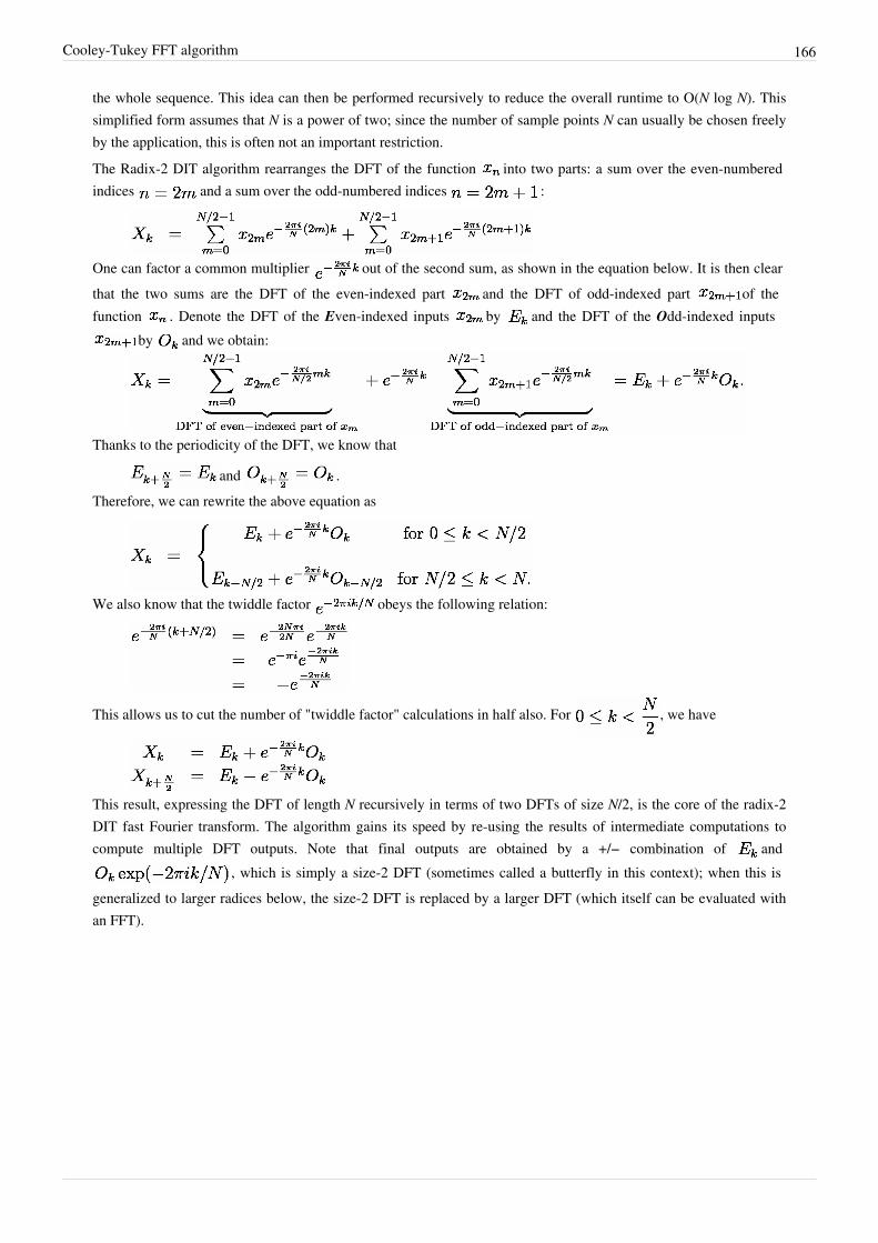
Cooley-Tukey FFT algorithm 166
the whole sequence. This idea can then be performed recursively to reduce the overall runtime to O(N log N). Thissimplified form assumes that N is a power of two; since the number of sample points N can usually be chosen freelyby the application, this is often not an important restriction.The Radix-2 DIT algorithm rearranges the DFT of the function into two parts: a sum over the even-numberedindices and a sum over the odd-numbered indices :
One can factor a common multiplier out of the second sum, as shown in the equation below. It is then clearthat the two sums are the DFT of the even-indexed part and the DFT of odd-indexed part of thefunction . Denote the DFT of the Even-indexed inputs by and the DFT of the Odd-indexed inputs
by and we obtain:
Thanks to the periodicity of the DFT, we know that
and .Therefore, we can rewrite the above equation as
We also know that the twiddle factor obeys the following relation:
This allows us to cut the number of "twiddle factor" calculations in half also. For , we have
This result, expressing the DFT of length N recursively in terms of two DFTs of size N/2, is the core of the radix-2DIT fast Fourier transform. The algorithm gains its speed by re-using the results of intermediate computations tocompute multiple DFT outputs. Note that final outputs are obtained by a +/− combination of and
, which is simply a size-2 DFT (sometimes called a butterfly in this context); when this isgeneralized to larger radices below, the size-2 DFT is replaced by a larger DFT (which itself can be evaluated withan FFT).
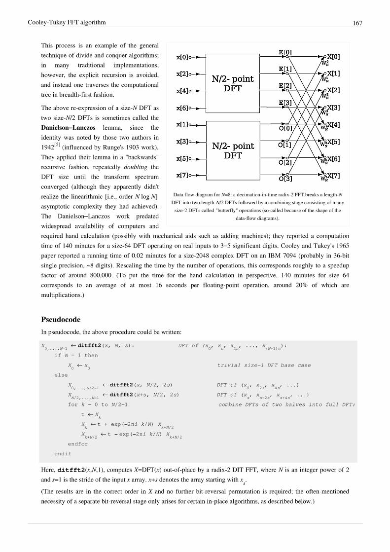
Cooley-Tukey FFT algorithm 167
Data flow diagram for N=8: a decimation-in-time radix-2 FFT breaks a length-NDFT into two length-N/2 DFTs followed by a combining stage consisting of many
size-2 DFTs called "butterfly" operations (so-called because of the shape of thedata-flow diagrams).
This process is an example of the generaltechnique of divide and conquer algorithms;in many traditional implementations,however, the explicit recursion is avoided,and instead one traverses the computationaltree in breadth-first fashion.
The above re-expression of a size-N DFT astwo size-N/2 DFTs is sometimes called theDanielson–Lanczos lemma, since theidentity was noted by those two authors in1942[5] (influenced by Runge's 1903 work).They applied their lemma in a "backwards"recursive fashion, repeatedly doubling theDFT size until the transform spectrumconverged (although they apparently didn'trealize the linearithmic [i.e., order N log N]asymptotic complexity they had achieved).The Danielson–Lanczos work predatedwidespread availability of computers andrequired hand calculation (possibly with mechanical aids such as adding machines); they reported a computationtime of 140 minutes for a size-64 DFT operating on real inputs to 3–5 significant digits. Cooley and Tukey's 1965paper reported a running time of 0.02 minutes for a size-2048 complex DFT on an IBM 7094 (probably in 36-bitsingle precision, ~8 digits). Rescaling the time by the number of operations, this corresponds roughly to a speedupfactor of around 800,000. (To put the time for the hand calculation in perspective, 140 minutes for size 64corresponds to an average of at most 16 seconds per floating-point operation, around 20% of which aremultiplications.)
PseudocodeIn pseudocode, the above procedure could be written:
X0,...,N−1 ← ditfft2(x, N, s): DFT of (x
0, x
s, x
2s, ..., x
(N-1)s):
if N = 1 then
X0 ← x
0 trivial size-1 DFT base case
else
X0,...,N/2−1 ← ditfft2(x, N/2, 2s) DFT of (x
0, x
2s, x
4s, ...)
XN/2,...,N−1 ← ditfft2(x+s, N/2, 2s) DFT of (x
s, x
s+2s, x
s+4s, ...)
for k = 0 to N/2−1 combine DFTs of two halves into full DFT: t ← X
k
Xk ← t + exp(−2πi k/N) X
k+N/2
Xk+N/2
← t − exp(−2πi k/N) Xk+N/2
endfor
endif
Here, ditfft2(x,N,1), computes X=DFT(x) out-of-place by a radix-2 DIT FFT, where N is an integer power of 2and s=1 is the stride of the input x array. x+s denotes the array starting with xs.(The results are in the correct order in X and no further bit-reversal permutation is required; the often-mentionednecessity of a separate bit-reversal stage only arises for certain in-place algorithms, as described below.)

Cooley-Tukey FFT algorithm 168
High-performance FFT implementations make many modifications to the implementation of such an algorithmcompared to this simple pseudocode. For example, one can use a larger base case than N=1 to amortize the overheadof recursion, the twiddle factors can be precomputed, and larger radices are often used for cachereasons; these and other optimizations together can improve the performance by an order of magnitude or more.[] (Inmany textbook implementations the depth-first recursion is eliminated entirely in favor of a nonrecursivebreadth-first approach, although depth-first recursion has been argued to have better memory locality.) Several ofthese ideas are described in further detail below.
General factorizations
The basic step of the Cooley–Tukey FFT for general factorizations can be viewed asre-interpreting a 1d DFT as something like a 2d DFT. The 1d input array of length N =N1N2 is reinterpreted as a 2d N1×N2 matrix stored in column-major order. One performs
smaller 1d DFTs along the N2 direction (the non-contiguous direction), then multiplies byphase factors (twiddle factors), and finally performs 1d DFTs along the N1 direction. Thetransposition step can be performed in the middle, as shown here, or at the beginning or
end. This is done recursively for the smaller transforms.
More generally, Cooley–Tukeyalgorithms recursively re-express aDFT of a composite size N = N1N2as:[6]
1. Perform N1 DFTs of size N2.2. Multiply by complex roots of unity
called twiddle factors.3. Perform N2 DFTs of size N1.Typically, either N1 or N2 is a smallfactor (not necessarily prime), calledthe radix (which can differ betweenstages of the recursion). If N1 is theradix, it is called a decimation in time(DIT) algorithm, whereas if N2 is theradix, it is decimation in frequency(DIF, also called the Sande-Tukeyalgorithm). The version presentedabove was a radix-2 DIT algorithm; inthe final expression, the phasemultiplying the odd transform is thetwiddle factor, and the +/- combination (butterfly) of the even and odd transforms is a size-2 DFT. (The radix's smallDFT is sometimes known as a butterfly, so-called because of the shape of the dataflow diagram for the radix-2 case.)
There are many other variations on the Cooley–Tukey algorithm. Mixed-radix implementations handle compositesizes with a variety of (typically small) factors in addition to two, usually (but not always) employing the O(N2)algorithm for the prime base cases of the recursion (it is also possible to employ an N log N algorithm for the primebase cases, such as Rader's or Bluestein's algorithm). Split radix merges radices 2 and 4, exploiting the fact that thefirst transform of radix 2 requires no twiddle factor, in order to achieve what was long the lowest known arithmeticoperation count for power-of-two sizes, although recent variations achieve an even lower count.[7][8] (On present-daycomputers, performance is determined more by cache and CPU pipeline considerations than by strict operationcounts; well-optimized FFT implementations often employ larger radices and/or hard-coded base-case transforms ofsignificant size.) Another way of looking at the Cooley–Tukey algorithm is that it re-expresses a size None-dimensional DFT as an N1 by N2 two-dimensional DFT (plus twiddles), where the output matrix is transposed.The net result of all of these transpositions, for a radix-2 algorithm, corresponds to a bit reversal of the input (DIF) oroutput (DIT) indices. If, instead of using a small radix, one employs a radix of roughly √N and explicit input/output
matrix transpositions, it is called a four-step algorithm (or six-step, depending on the number of transpositions), initially proposed to improve memory locality,[9][10] e.g. for cache optimization or out-of-core operation, and was
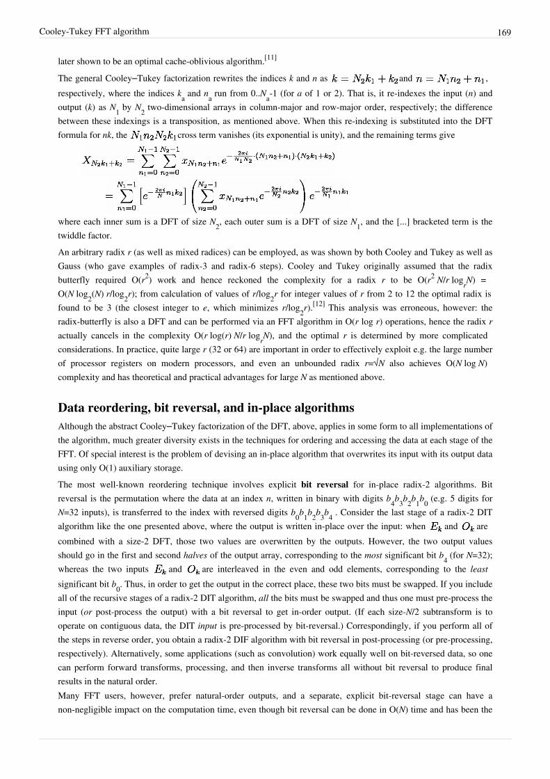
Cooley-Tukey FFT algorithm 169
later shown to be an optimal cache-oblivious algorithm.[11]
The general Cooley–Tukey factorization rewrites the indices k and n as and ,respectively, where the indices ka and na run from 0..Na-1 (for a of 1 or 2). That is, it re-indexes the input (n) andoutput (k) as N1 by N2 two-dimensional arrays in column-major and row-major order, respectively; the differencebetween these indexings is a transposition, as mentioned above. When this re-indexing is substituted into the DFTformula for nk, the cross term vanishes (its exponential is unity), and the remaining terms give
where each inner sum is a DFT of size N2, each outer sum is a DFT of size N1, and the [...] bracketed term is thetwiddle factor.An arbitrary radix r (as well as mixed radices) can be employed, as was shown by both Cooley and Tukey as well asGauss (who gave examples of radix-3 and radix-6 steps). Cooley and Tukey originally assumed that the radixbutterfly required O(r2) work and hence reckoned the complexity for a radix r to be O(r2 N/r logrN) =O(N log2(N) r/log2r); from calculation of values of r/log2r for integer values of r from 2 to 12 the optimal radix isfound to be 3 (the closest integer to e, which minimizes r/log2r).[12] This analysis was erroneous, however: theradix-butterfly is also a DFT and can be performed via an FFT algorithm in O(r log r) operations, hence the radix ractually cancels in the complexity O(r log(r) N/r logrN), and the optimal r is determined by more complicatedconsiderations. In practice, quite large r (32 or 64) are important in order to effectively exploit e.g. the large numberof processor registers on modern processors, and even an unbounded radix r=√N also achieves O(N log N)complexity and has theoretical and practical advantages for large N as mentioned above.
Data reordering, bit reversal, and in-place algorithmsAlthough the abstract Cooley–Tukey factorization of the DFT, above, applies in some form to all implementations ofthe algorithm, much greater diversity exists in the techniques for ordering and accessing the data at each stage of theFFT. Of special interest is the problem of devising an in-place algorithm that overwrites its input with its output datausing only O(1) auxiliary storage.The most well-known reordering technique involves explicit bit reversal for in-place radix-2 algorithms. Bitreversal is the permutation where the data at an index n, written in binary with digits b4b3b2b1b0 (e.g. 5 digits forN=32 inputs), is transferred to the index with reversed digits b0b1b2b3b4 . Consider the last stage of a radix-2 DITalgorithm like the one presented above, where the output is written in-place over the input: when and arecombined with a size-2 DFT, those two values are overwritten by the outputs. However, the two output valuesshould go in the first and second halves of the output array, corresponding to the most significant bit b4 (for N=32);whereas the two inputs and are interleaved in the even and odd elements, corresponding to the leastsignificant bit b0. Thus, in order to get the output in the correct place, these two bits must be swapped. If you includeall of the recursive stages of a radix-2 DIT algorithm, all the bits must be swapped and thus one must pre-process theinput (or post-process the output) with a bit reversal to get in-order output. (If each size-N/2 subtransform is tooperate on contiguous data, the DIT input is pre-processed by bit-reversal.) Correspondingly, if you perform all ofthe steps in reverse order, you obtain a radix-2 DIF algorithm with bit reversal in post-processing (or pre-processing,respectively). Alternatively, some applications (such as convolution) work equally well on bit-reversed data, so onecan perform forward transforms, processing, and then inverse transforms all without bit reversal to produce finalresults in the natural order.Many FFT users, however, prefer natural-order outputs, and a separate, explicit bit-reversal stage can have a non-negligible impact on the computation time, even though bit reversal can be done in O(N) time and has been the

Cooley-Tukey FFT algorithm 170
subject of much research. Also, while the permutation is a bit reversal in the radix-2 case, it is more generally anarbitrary (mixed-base) digit reversal for the mixed-radix case, and the permutation algorithms become morecomplicated to implement. Moreover, it is desirable on many hardware architectures to re-order intermediate stagesof the FFT algorithm so that they operate on consecutive (or at least more localized) data elements. To these ends, anumber of alternative implementation schemes have been devised for the Cooley–Tukey algorithm that do notrequire separate bit reversal and/or involve additional permutations at intermediate stages.The problem is greatly simplified if it is out-of-place: the output array is distinct from the input array or,equivalently, an equal-size auxiliary array is available. The Stockham auto-sort algorithm[13] performs every stageof the FFT out-of-place, typically writing back and forth between two arrays, transposing one "digit" of the indiceswith each stage, and has been especially popular on SIMD architectures.[] Even greater potential SIMD advantages(more consecutive accesses) have been proposed for the Pease algorithm, which also reorders out-of-place with eachstage, but this method requires separate bit/digit reversal and O(N log N) storage. One can also directly apply theCooley–Tukey factorization definition with explicit (depth-first) recursion and small radices, which producesnatural-order out-of-place output with no separate permutation step (as in the pseudocode above) and can be arguedto have cache-oblivious locality benefits on systems with hierarchical memory.[14]
A typical strategy for in-place algorithms without auxiliary storage and without separate digit-reversal passesinvolves small matrix transpositions (which swap individual pairs of digits) at intermediate stages, which can becombined with the radix butterflies to reduce the number of passes over the data.
References[1] Gauss, Carl Friedrich, " Theoria interpolationis methodo nova tractata (http:/ / lseet. univ-tln. fr/ ~iaroslav/
Gauss_Theoria_interpolationis_methodo_nova_tractata. php)", Werke, Band 3, 265–327 (Königliche Gesellschaft der Wissenschaften,Göttingen, 1866)
[2] Heideman, M. T., D. H. Johnson, and C. S. Burrus, " Gauss and the history of the fast Fourier transform (http:/ / ieeexplore. ieee. org/ xpls/abs_all. jsp?arnumber=1162257)," IEEE ASSP Magazine, 1, (4), 14–21 (1984)
[3] Rockmore, Daniel N. , Comput. Sci. Eng. 2 (1), 60 (2000). The FFT — an algorithm the whole family can use (http:/ / www. cs. dartmouth.edu/ ~rockmore/ cse-fft. pdf) Special issue on "top ten algorithms of the century " (http:/ / amath. colorado. edu/ resources/ archive/ topten.pdf)
[4] James W. Cooley, Peter A. W. Lewis, and Peter W. Welch, "Historical notes on the fast Fourier transform," Proc. IEEE, vol. 55 (no. 10), p.1675–1677 (1967).
[5] Danielson, G. C., and C. Lanczos, "Some improvements in practical Fourier analysis and their application to X-ray scattering from liquids," J.Franklin Inst. 233, 365–380 and 435–452 (1942).
[6] Duhamel, P., and M. Vetterli, "Fast Fourier transforms: a tutorial review and a state of the art," Signal Processing 19, 259–299 (1990)[7] Lundy, T., and J. Van Buskirk, "A new matrix approach to real FFTs and convolutions of length 2k," Computing 80, 23-45 (2007).[8] Johnson, S. G., and M. Frigo, " A modified split-radix FFT with fewer arithmetic operations (http:/ / www. fftw. org/ newsplit. pdf)," IEEE
Trans. Signal Processing 55 (1), 111–119 (2007).[9] Gentleman W. M., and G. Sande, "Fast Fourier transforms—for fun and profit," Proc. AFIPS 29, 563–578 (1966).[10] Bailey, David H., "FFTs in external or hierarchical memory," J. Supercomputing 4 (1), 23–35 (1990)[11] M. Frigo, C.E. Leiserson, H. Prokop, and S. Ramachandran. Cache-oblivious algorithms. In Proceedings of the 40th IEEE Symposium on
Foundations of Computer Science (FOCS 99), p.285-297. 1999. Extended abstract at IEEE (http:/ / ieeexplore. ieee. org/ iel5/ 6604/ 17631/00814600. pdf?arnumber=814600), at Citeseer (http:/ / citeseer. ist. psu. edu/ 307799. html).
[12] Cooley, J. W., P. Lewis and P. Welch, "The Fast Fourier Transform and its Applications", IEEE Trans on Education 12, 1, 28-34 (1969)[13] Originally attributed to Stockham in W. T. Cochran et al., What is the fast Fourier transform? (http:/ / dx. doi. org/ 10. 1109/ PROC. 1967.
5957), Proc. IEEE vol. 55, 1664–1674 (1967).[14] A free (GPL) C library for computing discrete Fourier transforms in one or more dimensions, of arbitrary size, using the Cooley–Tukey
algorithm
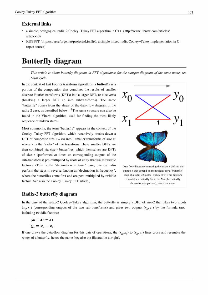
Cooley-Tukey FFT algorithm 171
External links• a simple, pedagogical radix-2 Cooley–Tukey FFT algorithm in C++. (http:/ / www. librow. com/ articles/
article-10)• KISSFFT (http:/ / sourceforge. net/ projects/ kissfft/ ): a simple mixed-radix Cooley–Tukey implementation in C
(open source)
Butterfly diagramThis article is about butterfly diagrams in FFT algorithms; for the sunspot diagrams of the same name, seeSolar cycle.
Data flow diagram connecting the inputs x (left) to theoutputs y that depend on them (right) for a "butterfly"step of a radix-2 Cooley–Tukey FFT. This diagram
resembles a butterfly (as in the Morpho butterflyshown for comparison), hence the name.
In the context of fast Fourier transform algorithms, a butterfly is aportion of the computation that combines the results of smallerdiscrete Fourier transforms (DFTs) into a larger DFT, or vice versa(breaking a larger DFT up into subtransforms). The name"butterfly" comes from the shape of the data-flow diagram in theradix-2 case, as described below.[1] The same structure can also befound in the Viterbi algorithm, used for finding the most likelysequence of hidden states.
Most commonly, the term "butterfly" appears in the context of theCooley–Tukey FFT algorithm, which recursively breaks down aDFT of composite size n = rm into r smaller transforms of size mwhere r is the "radix" of the transform. These smaller DFTs arethen combined via size-r butterflies, which themselves are DFTsof size r (performed m times on corresponding outputs of thesub-transforms) pre-multiplied by roots of unity (known as twiddlefactors). (This is the "decimation in time" case; one can alsoperform the steps in reverse, known as "decimation in frequency",where the butterflies come first and are post-multiplied by twiddlefactors. See also the Cooley–Tukey FFT article.)
Radix-2 butterfly diagram
In the case of the radix-2 Cooley–Tukey algorithm, the butterfly is simply a DFT of size-2 that takes two inputs(x0, x1) (corresponding outputs of the two sub-transforms) and gives two outputs (y0, y1) by the formula (notincluding twiddle factors):
If one draws the data-flow diagram for this pair of operations, the (x0, x1) to (y0, y1) lines cross and resemble thewings of a butterfly, hence the name (see also the illustration at right).

Butterfly diagram 172
A decimation-in-time radix-2 FFT breaks a length-N DFT into two length-N/2DFTs followed by a combining stage consisting of many butterfly operations.
More specifically, a decimation-in-time FFTalgorithm on n = 2 p inputs with respect to aprimitive n-th root of unity
relies on O(n log n) butterflies of the form:
where k is an integer depending on the partof the transform being computed. Whereasthe corresponding inverse transform canmathematically be performed by replacing ωwith ω−1 (and possibly multiplying by anoverall scale factor, depending on thenormalization convention), one may alsodirectly invert the butterflies:
corresponding to a decimation-in-frequency FFT algorithm.
Other usesThe butterfly can also be used to improve the randomness of large arrays of partially random numbers, by bringingevery 32 or 64 bit word into causal contact with every other word through a desired hashing algorithm, so that achange in any one bit has the possibility of changing all the bits in the large array.
References[1] Alan V. Oppenheim, Ronald W. Schafer, and John R. Buck, Discrete-Time Signal Processing, 2nd edition (Upper Saddle River, NJ: Prentice
Hall, 1989)
External links• explanation of the FFT and butterfly diagrams (http:/ / www. relisoft. com/ Science/ Physics/ fft. html).• butterfly diagrams of various FFT implementations (Radix-2, Radix-4, Split-Radix) (http:/ / www. cmlab. csie.
ntu. edu. tw/ cml/ dsp/ training/ coding/ transform/ fft. html).

Codec 173
CodecThis article is about encoding and decoding a digital data stream. For other uses, see Codec (disambiguation).Further information: List of codecs and Video codecsA codec is a device or computer program capable of encoding or decoding a digital data stream or signal. The wordcodec is a portmanteau of "coder-decoder" or, less commonly, "compressor-decompressor". A codec (the program)should not be confused with a coding or compression format or standard – a format is a document (the standard), away of storing data, while a codec is a program (an implementation) which can read or write such files. In practice,however, "codec" is sometimes used loosely to refer to formats.A codec encodes a data stream or signal for transmission, storage or encryption, or decodes it for playback orediting. Codecs are used in videoconferencing, streaming media and video editing applications. A video camera'sanalog-to-digital converter (ADC) converts its analog signals into digital signals, which are then passed through avideo compressor for digital transmission or storage. A receiving device then runs the signal through a videodecompressor, then a digital-to-analog converter (DAC) for analog display. The term codec is also used as a genericname for a videoconferencing unit.
Related conceptsAn endec (encoder/decoder) is a similar yet different concept mainly used for hardware. In the mid 20th century, a"codec" was hardware that coded analog signals into pulse-code modulation (PCM) and decoded them back. Late inthe century the name came to be applied to a class of software for converting among digital signal formats, andincluding compander functions.A modem is a contraction of modulator/demodulator (although they were referred to as "datasets" by telcos) andconverts digital data from computers to analog for phone line transmission. On the receiving end the analog isconverted back to digital. Codecs do the opposite (convert audio analog to digital and then computer digital soundback to audio).An audio codec converts analog audio signals into digital signals for transmission or storage. A receiving device thenconverts the digital signals back to analog using an audio decompressor, for playback. An example of this is thecodecs used in the sound cards of personal computers. A video codec accomplishes the same task for video signals.
Compression quality• Lossy codecs: Many of the more popular codecs in the software world are lossy, meaning that they reduce quality
by some amount in order to achieve compression. Often, this type of compression is virtually indistinguishablefrom the original uncompressed sound or images, depending on the codec and the settings used. Smaller data setsease the strain on relatively expensive storage sub-systems such as non-volatile memory and hard disk, as well aswrite-once-read-many formats such as CD-ROM, DVD and Blu-ray Disc. Lower data rates also reduce cost andimprove performance when the data is transmitted.
• Lossless codecs: There are also many lossless codecs which are typically used for archiving data in a compressedform while retaining all of the information present in the original stream. If preserving the original quality of thestream is more important than eliminating the correspondingly larger data sizes, lossless codecs are preferred.This is especially true if the data is to undergo further processing (for example editing) in which case the repeatedapplication of processing (encoding and decoding) on lossy codecs will degrade the quality of the resulting datasuch that it is no longer identifiable (visually, audibly or both). Using more than one codec or encoding schemesuccessively can also degrade quality significantly. The decreasing cost of storage capacity and networkbandwidth has a tendency to reduce the need for lossy codecs for some media.
Codec 174
Media codecsTwo principal techniques are used in codecs, pulse-code modulation and delta modulation. Codecs are oftendesigned to emphasize certain aspects of the media to be encoded. For example, a digital video (using a DV codec)of a sports event needs to encode motion well but not necessarily exact colors, while a video of an art exhibit needsto encode color and surface texture well.Audio codecs for cell phones need to have very low latency between source encoding and playback. In contrast,audio codecs for recording or broadcast can use high-latency audio compression techniques to achieve higher fidelityat a lower bit-rate.There are thousands of audio and video codecs, ranging in cost from free to hundreds of dollars or more. This varietyof codecs can create compatibility and obsolescence issues. The impact is lessened for older formats, for which freeor nearly-free codecs have existed for a long time. The older formats are often ill-suited to modern applications,however, such as playback in small portable devices. For example, raw uncompressed PCM audio (44.1 kHz, 16 bitstereo, as represented on an audio CD or in a .wav or .aiff file) has long been a standard across multiple platforms,but its transmission over networks is slow and expensive compared with more modern compressed formats, such asMP3.Many multimedia data streams contain both audio and video, and often some metadata that permit synchronizationof audio and video. Each of these three streams may be handled by different programs, processes, or hardware; butfor the multimedia data streams to be useful in stored or transmitted form, they must be encapsulated together in acontainer format.Lower bitrate codecs allow more users, but they also have more distortion. Beyond the initial increase in distortion,lower bit rate codecs also achieve their lower bit rates by using more complex algorithms that make certainassumptions, such as those about the media and the packet loss rate. Other codecs may not make those sameassumptions. When a user with a low bitrate codec talks to a user with another codec, additional distortion isintroduced by each transcoding.AVI is sometimes erroneously described as a codec, but AVI is actually a container format, while a codec is asoftware or hardware tool that encodes or decodes audio or video into or from some audio or video format. Audioand video encoded with many codecs might be put into an AVI container, although AVI is not an ISO standard.There are also other well-known container formats, such as Ogg, ASF, QuickTime, RealMedia, Matroska, and DivXMedia Format. Some container formats which are ISO standards are MPEG transport stream, MPEG programstream, MP4 and ISO base media file format.
References
FFTW 175
FFTW
FFTW
Developer(s) Matteo Frigo and Steven G. Johnson
Initial release 24 March 1997
Stable release 3.3.4 / 16 March 2014
Written in C, OCaml
Type Numerical software
License GPL, commercial
Website www.fftw.org [1]
The Fastest Fourier Transform in the West (FFTW) is a software library for computing discrete Fouriertransforms (DFTs) developed by Matteo Frigo and Steven G. Johnson at the Massachusetts Institute of Technology.FFTW is known as the fastest free software implementation of the Fast Fourier transform (FFT) algorithm (upheldby regular benchmarks[2]). It can compute transforms of real and complex-valued arrays of arbitrary size anddimension in O(n log n) time.It does this by supporting a variety of algorithms and choosing the one (a particular decomposition of the transforminto smaller transforms) it estimates or measures to be preferable in the particular circumstances. It works best onarrays of sizes with small prime factors, with powers of two being optimal and large primes being worst case (butstill O(n log n)). To decompose transforms of composite sizes into smaller transforms, it chooses among severalvariants of the Cooley–Tukey FFT algorithm (corresponding to different factorizations and/or differentmemory-access patterns), while for prime sizes it uses either Rader's or Bluestein's FFT algorithm. Once thetransform has been broken up into subtransforms of sufficiently small sizes, FFTW uses hard-coded unrolled FFTsfor these small sizes that were produced (at compile time, not at run time) by code generation; these routines use avariety of algorithms including Cooley–Tukey variants, Rader's algorithm, and prime-factor FFT algorithms.For a sufficiently large number of repeated transforms it is advantageous to measure the performance of some or allof the supported algorithms on the given array size and platform. These measurements, which the authors refer to as"wisdom", can be stored in a file or string for later use.FFTW has a "guru interface" that intends "to expose as much as possible of the flexibility in the underlying FFTWarchitecture". This allows, among other things, multi-dimensional transforms and multiple transforms in a single call(e.g., where the data is interleaved in memory).FFTW has limited support for out-of-order transforms (using the MPI version). The data reordering incurs anoverhead, which for in-place transforms of arbitrary size and dimension is non-trivial to avoid. It is undocumentedfor which transforms this overhead is significant.FFTW is licensed under the GNU General Public License. It is also licensed commercially by MIT and is used in thecommercial MATLAB[3] matrix package for calculating FFTs. FFTW is written in the C language, but Fortran andAda interfaces exist, as well as interfaces for a few other languages. While the library itself is C, the code is actuallygenerated from a program called 'genfft', which is written in OCaml.[4]
In 1999, FFTW won the J. H. Wilkinson Prize for Numerical Software.

FFTW 176
References[1] http:/ / www. fftw. org/[2] Homepage, second paragraph (http:/ / www. fftw. org/ ), and benchmarks page (http:/ / www. fftw. org/ benchfft/ )[3] Faster Finite Fourier Transforms: MATLAB 6 incorporates FFTW (http:/ / www. mathworks. com/ company/ newsletters/ articles/
faster-finite-fourier-transforms-matlab. html)[4] "FFTW FAQ" (http:/ / www. fftw. org/ faq/ section2. html#languages)
External links• Official website (http:/ / www. fftw. org/ )
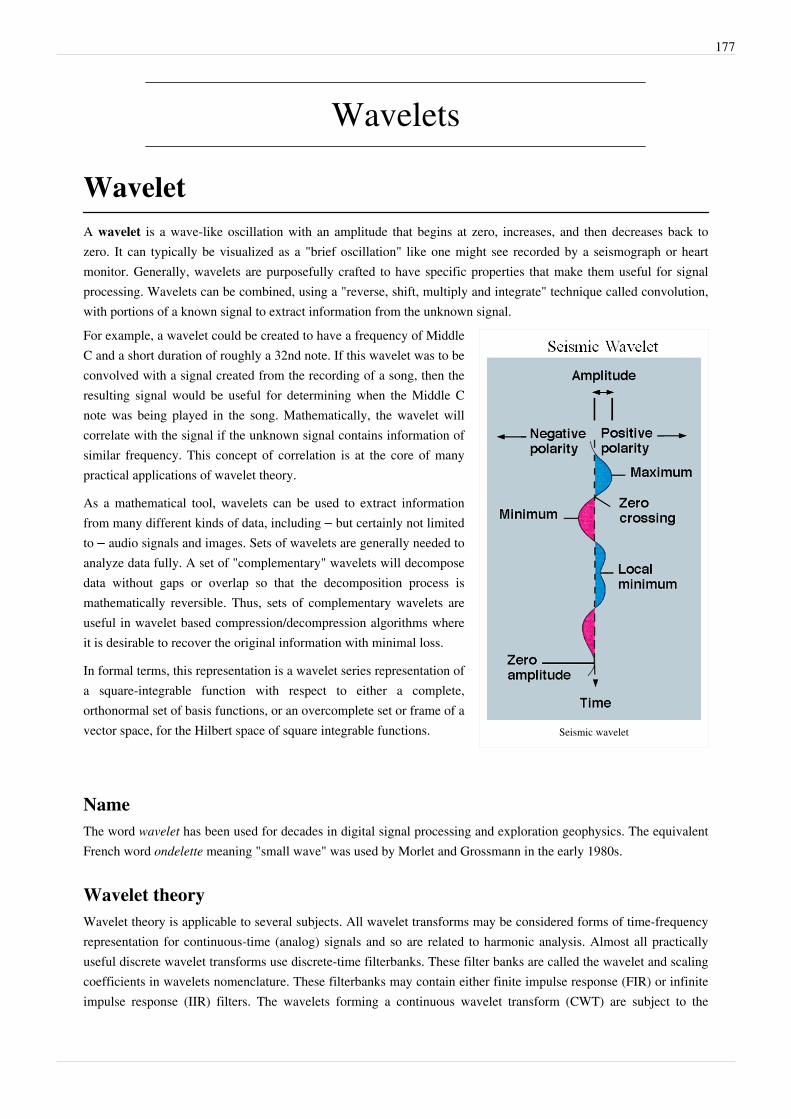
177
Wavelets
WaveletA wavelet is a wave-like oscillation with an amplitude that begins at zero, increases, and then decreases back tozero. It can typically be visualized as a "brief oscillation" like one might see recorded by a seismograph or heartmonitor. Generally, wavelets are purposefully crafted to have specific properties that make them useful for signalprocessing. Wavelets can be combined, using a "reverse, shift, multiply and integrate" technique called convolution,with portions of a known signal to extract information from the unknown signal.
Seismic wavelet
For example, a wavelet could be created to have a frequency of MiddleC and a short duration of roughly a 32nd note. If this wavelet was to beconvolved with a signal created from the recording of a song, then theresulting signal would be useful for determining when the Middle Cnote was being played in the song. Mathematically, the wavelet willcorrelate with the signal if the unknown signal contains information ofsimilar frequency. This concept of correlation is at the core of manypractical applications of wavelet theory.
As a mathematical tool, wavelets can be used to extract informationfrom many different kinds of data, including – but certainly not limitedto – audio signals and images. Sets of wavelets are generally needed toanalyze data fully. A set of "complementary" wavelets will decomposedata without gaps or overlap so that the decomposition process ismathematically reversible. Thus, sets of complementary wavelets areuseful in wavelet based compression/decompression algorithms whereit is desirable to recover the original information with minimal loss.
In formal terms, this representation is a wavelet series representation ofa square-integrable function with respect to either a complete,orthonormal set of basis functions, or an overcomplete set or frame of avector space, for the Hilbert space of square integrable functions.
NameThe word wavelet has been used for decades in digital signal processing and exploration geophysics. The equivalentFrench word ondelette meaning "small wave" was used by Morlet and Grossmann in the early 1980s.
Wavelet theoryWavelet theory is applicable to several subjects. All wavelet transforms may be considered forms of time-frequency representation for continuous-time (analog) signals and so are related to harmonic analysis. Almost all practically useful discrete wavelet transforms use discrete-time filterbanks. These filter banks are called the wavelet and scaling coefficients in wavelets nomenclature. These filterbanks may contain either finite impulse response (FIR) or infinite impulse response (IIR) filters. The wavelets forming a continuous wavelet transform (CWT) are subject to the
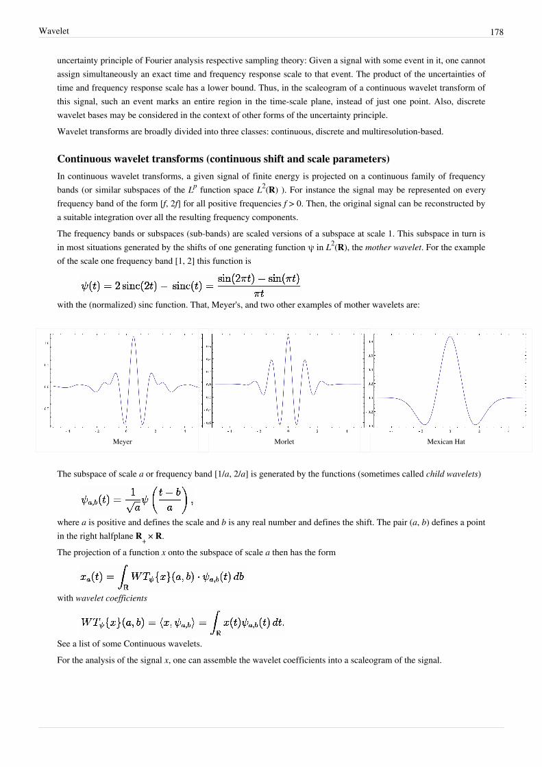
Wavelet 178
uncertainty principle of Fourier analysis respective sampling theory: Given a signal with some event in it, one cannotassign simultaneously an exact time and frequency response scale to that event. The product of the uncertainties oftime and frequency response scale has a lower bound. Thus, in the scaleogram of a continuous wavelet transform ofthis signal, such an event marks an entire region in the time-scale plane, instead of just one point. Also, discretewavelet bases may be considered in the context of other forms of the uncertainty principle.Wavelet transforms are broadly divided into three classes: continuous, discrete and multiresolution-based.
Continuous wavelet transforms (continuous shift and scale parameters)In continuous wavelet transforms, a given signal of finite energy is projected on a continuous family of frequencybands (or similar subspaces of the Lp function space L2(R) ). For instance the signal may be represented on everyfrequency band of the form [f, 2f] for all positive frequencies f > 0. Then, the original signal can be reconstructed bya suitable integration over all the resulting frequency components.The frequency bands or subspaces (sub-bands) are scaled versions of a subspace at scale 1. This subspace in turn isin most situations generated by the shifts of one generating function ψ in L2(R), the mother wavelet. For the exampleof the scale one frequency band [1, 2] this function is
with the (normalized) sinc function. That, Meyer's, and two other examples of mother wavelets are:
Meyer Morlet Mexican Hat
The subspace of scale a or frequency band [1/a, 2/a] is generated by the functions (sometimes called child wavelets)
where a is positive and defines the scale and b is any real number and defines the shift. The pair (a, b) defines a pointin the right halfplane R+ × R.The projection of a function x onto the subspace of scale a then has the form
with wavelet coefficients
See a list of some Continuous wavelets.For the analysis of the signal x, one can assemble the wavelet coefficients into a scaleogram of the signal.
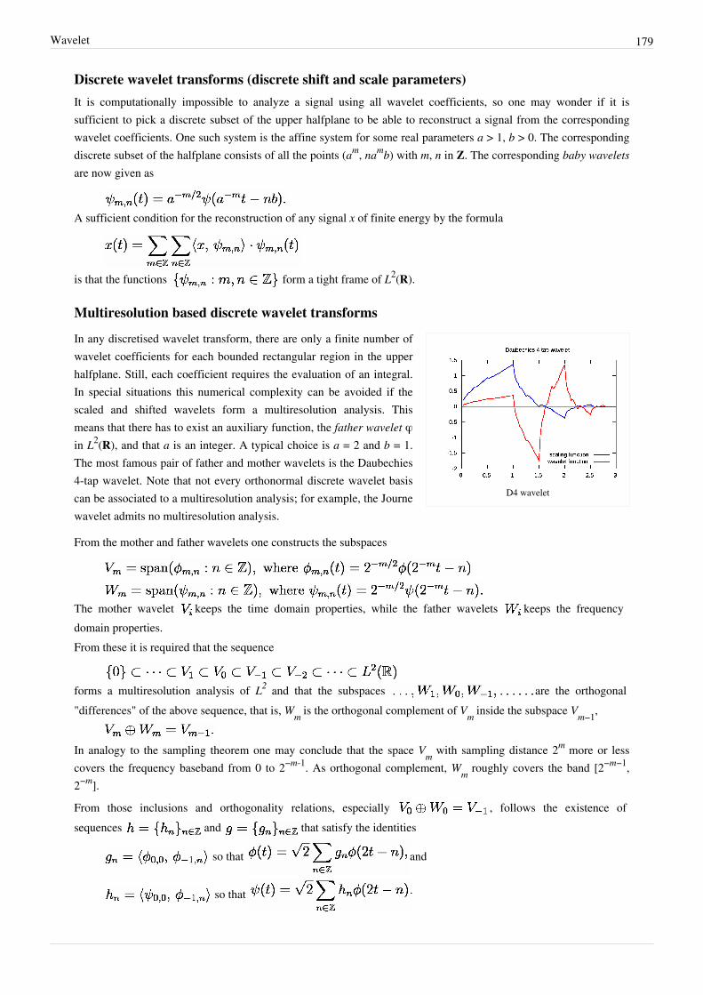
Wavelet 179
Discrete wavelet transforms (discrete shift and scale parameters)It is computationally impossible to analyze a signal using all wavelet coefficients, so one may wonder if it issufficient to pick a discrete subset of the upper halfplane to be able to reconstruct a signal from the correspondingwavelet coefficients. One such system is the affine system for some real parameters a > 1, b > 0. The correspondingdiscrete subset of the halfplane consists of all the points (am, namb) with m, n in Z. The corresponding baby waveletsare now given as
A sufficient condition for the reconstruction of any signal x of finite energy by the formula
is that the functions form a tight frame of L2(R).
Multiresolution based discrete wavelet transforms
D4 wavelet
In any discretised wavelet transform, there are only a finite number ofwavelet coefficients for each bounded rectangular region in the upperhalfplane. Still, each coefficient requires the evaluation of an integral.In special situations this numerical complexity can be avoided if thescaled and shifted wavelets form a multiresolution analysis. Thismeans that there has to exist an auxiliary function, the father wavelet φin L2(R), and that a is an integer. A typical choice is a = 2 and b = 1.The most famous pair of father and mother wavelets is the Daubechies4-tap wavelet. Note that not every orthonormal discrete wavelet basiscan be associated to a multiresolution analysis; for example, the Journewavelet admits no multiresolution analysis.
From the mother and father wavelets one constructs the subspaces
The mother wavelet keeps the time domain properties, while the father wavelets keeps the frequencydomain properties.From these it is required that the sequence
forms a multiresolution analysis of L2 and that the subspaces are the orthogonal"differences" of the above sequence, that is, Wm is the orthogonal complement of Vm inside the subspace Vm−1,
In analogy to the sampling theorem one may conclude that the space Vm with sampling distance 2m more or lesscovers the frequency baseband from 0 to 2−m-1. As orthogonal complement, Wm roughly covers the band [2−m−1,2−m].
From those inclusions and orthogonality relations, especially , follows the existence ofsequences and that satisfy the identities
so that and
so that
Wavelet 180
The second identity of the first pair is a refinement equation for the father wavelet φ. Both pairs of identities formthe basis for the algorithm of the fast wavelet transform.From the multiresolution analysis derives the orthogonal decomposition of the space L2 as
For any signal or function this gives a representation in basis functions of the corresponding subspaces as
where the coefficients are
and.
Mother waveletFor practical applications, and for efficiency reasons, one prefers continuously differentiable functions with compactsupport as mother (prototype) wavelet (functions). However, to satisfy analytical requirements (in the continuousWT) and in general for theoretical reasons, one chooses the wavelet functions from a subspace of the space
This is the space of measurable functions that are absolutely and square integrable:
and
Being in this space ensures that one can formulate the conditions of zero mean and square norm one:
is the condition for zero mean, and
is the condition for square norm one.
For ψ to be a wavelet for the continuous wavelet transform (see there for exact statement), the mother wavelet mustsatisfy an admissibility criterion (loosely speaking, a kind of half-differentiability) in order to get a stably invertibletransform.For the discrete wavelet transform, one needs at least the condition that the wavelet series is a representation of theidentity in the space L2(R). Most constructions of discrete WT make use of the multiresolution analysis, whichdefines the wavelet by a scaling function. This scaling function itself is solution to a functional equation.In most situations it is useful to restrict ψ to be a continuous function with a higher number M of vanishing moments,i.e. for all integer m < M
The mother wavelet is scaled (or dilated) by a factor of a and translated (or shifted) by a factor of b to give (underMorlet's original formulation):
For the continuous WT, the pair (a,b) varies over the full half-plane R+ × R; for the discrete WT this pair varies overa discrete subset of it, which is also called affine group.These functions are often incorrectly referred to as the basis functions of the (continuous) transform. In fact, as in thecontinuous Fourier transform, there is no basis in the continuous wavelet transform. Time-frequency interpretationuses a subtly different formulation (after Delprat).
Restriction:
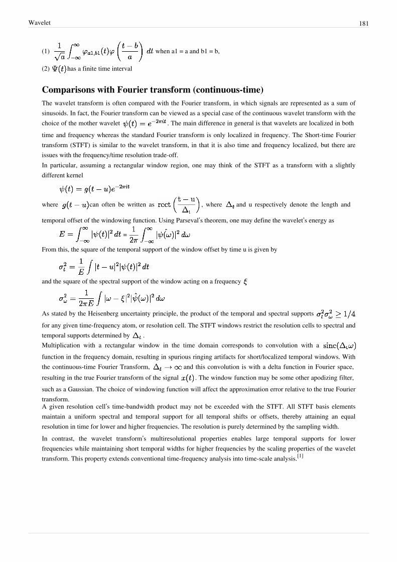
Wavelet 181
(1) when a1 = a and b1 = b,
(2) has a finite time interval
Comparisons with Fourier transform (continuous-time)The wavelet transform is often compared with the Fourier transform, in which signals are represented as a sum ofsinusoids. In fact, the Fourier transform can be viewed as a special case of the continuous wavelet transform with thechoice of the mother wavelet . The main difference in general is that wavelets are localized in bothtime and frequency whereas the standard Fourier transform is only localized in frequency. The Short-time Fouriertransform (STFT) is similar to the wavelet transform, in that it is also time and frequency localized, but there areissues with the frequency/time resolution trade-off.In particular, assuming a rectangular window region, one may think of the STFT as a transform with a slightlydifferent kernel
where can often be written as , where and u respectively denote the length and
temporal offset of the windowing function. Using Parseval’s theorem, one may define the wavelet’s energy as
=
From this, the square of the temporal support of the window offset by time u is given by
and the square of the spectral support of the window acting on a frequency
As stated by the Heisenberg uncertainty principle, the product of the temporal and spectral supports for any given time-frequency atom, or resolution cell. The STFT windows restrict the resolution cells to spectral andtemporal supports determined by .Multiplication with a rectangular window in the time domain corresponds to convolution with a function in the frequency domain, resulting in spurious ringing artifacts for short/localized temporal windows. Withthe continuous-time Fourier Transform, and this convolution is with a delta function in Fourier space,resulting in the true Fourier transform of the signal . The window function may be some other apodizing filter,such as a Gaussian. The choice of windowing function will affect the approximation error relative to the true Fouriertransform.A given resolution cell’s time-bandwidth product may not be exceeded with the STFT. All STFT basis elementsmaintain a uniform spectral and temporal support for all temporal shifts or offsets, thereby attaining an equalresolution in time for lower and higher frequencies. The resolution is purely determined by the sampling width.In contrast, the wavelet transform’s multiresolutional properties enables large temporal supports for lowerfrequencies while maintaining short temporal widths for higher frequencies by the scaling properties of the wavelettransform. This property extends conventional time-frequency analysis into time-scale analysis.[1]
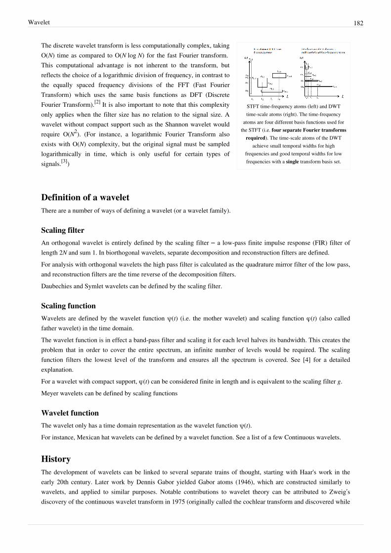
Wavelet 182
STFT time-frequency atoms (left) and DWTtime-scale atoms (right). The time-frequency
atoms are four different basis functions used forthe STFT (i.e. four separate Fourier transforms
required). The time-scale atoms of the DWTachieve small temporal widths for high
frequencies and good temporal widths for lowfrequencies with a single transform basis set.
The discrete wavelet transform is less computationally complex, takingO(N) time as compared to O(N log N) for the fast Fourier transform.This computational advantage is not inherent to the transform, butreflects the choice of a logarithmic division of frequency, in contrast tothe equally spaced frequency divisions of the FFT (Fast FourierTransform) which uses the same basis functions as DFT (DiscreteFourier Transform).[2] It is also important to note that this complexityonly applies when the filter size has no relation to the signal size. Awavelet without compact support such as the Shannon wavelet wouldrequire O(N2). (For instance, a logarithmic Fourier Transform alsoexists with O(N) complexity, but the original signal must be sampledlogarithmically in time, which is only useful for certain types ofsignals.[3])
Definition of a waveletThere are a number of ways of defining a wavelet (or a wavelet family).
Scaling filterAn orthogonal wavelet is entirely defined by the scaling filter – a low-pass finite impulse response (FIR) filter oflength 2N and sum 1. In biorthogonal wavelets, separate decomposition and reconstruction filters are defined.For analysis with orthogonal wavelets the high pass filter is calculated as the quadrature mirror filter of the low pass,and reconstruction filters are the time reverse of the decomposition filters.Daubechies and Symlet wavelets can be defined by the scaling filter.
Scaling functionWavelets are defined by the wavelet function ψ(t) (i.e. the mother wavelet) and scaling function φ(t) (also calledfather wavelet) in the time domain.The wavelet function is in effect a band-pass filter and scaling it for each level halves its bandwidth. This creates theproblem that in order to cover the entire spectrum, an infinite number of levels would be required. The scalingfunction filters the lowest level of the transform and ensures all the spectrum is covered. See [4] for a detailedexplanation.For a wavelet with compact support, φ(t) can be considered finite in length and is equivalent to the scaling filter g.Meyer wavelets can be defined by scaling functions
Wavelet functionThe wavelet only has a time domain representation as the wavelet function ψ(t).For instance, Mexican hat wavelets can be defined by a wavelet function. See a list of a few Continuous wavelets.
HistoryThe development of wavelets can be linked to several separate trains of thought, starting with Haar's work in the early 20th century. Later work by Dennis Gabor yielded Gabor atoms (1946), which are constructed similarly to wavelets, and applied to similar purposes. Notable contributions to wavelet theory can be attributed to Zweig’s discovery of the continuous wavelet transform in 1975 (originally called the cochlear transform and discovered while
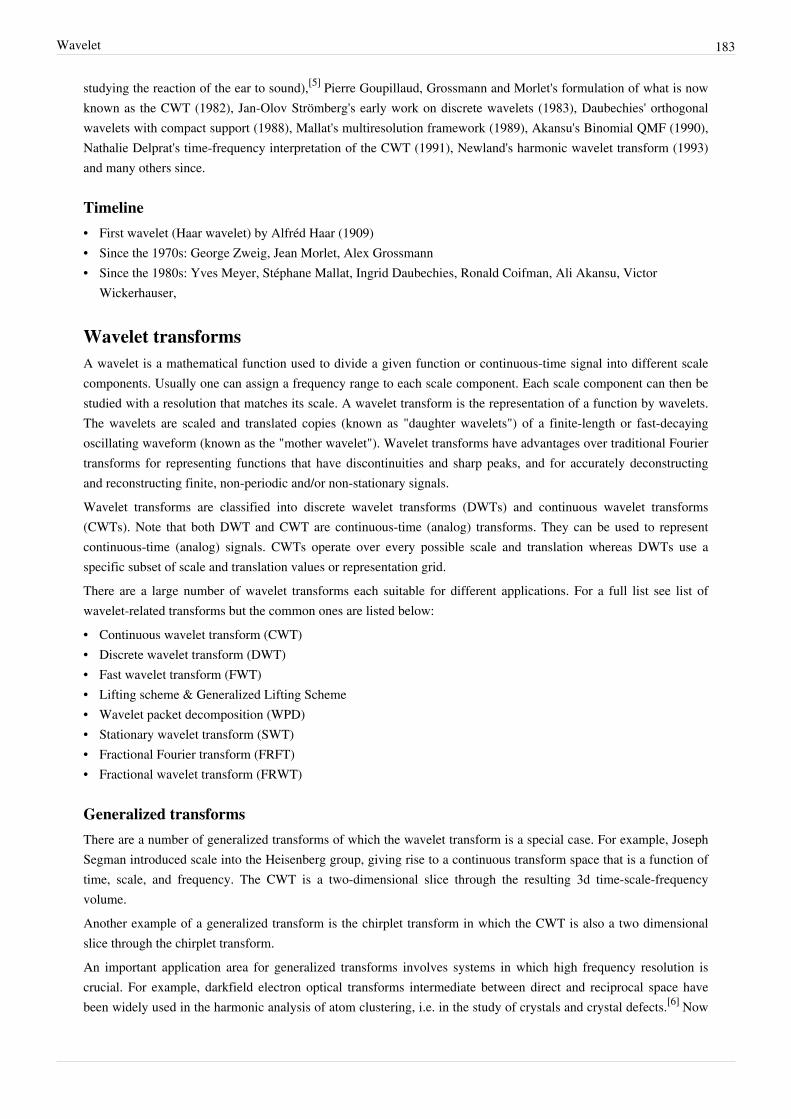
Wavelet 183
studying the reaction of the ear to sound),[5] Pierre Goupillaud, Grossmann and Morlet's formulation of what is nowknown as the CWT (1982), Jan-Olov Strömberg's early work on discrete wavelets (1983), Daubechies' orthogonalwavelets with compact support (1988), Mallat's multiresolution framework (1989), Akansu's Binomial QMF (1990),Nathalie Delprat's time-frequency interpretation of the CWT (1991), Newland's harmonic wavelet transform (1993)and many others since.
Timeline• First wavelet (Haar wavelet) by Alfréd Haar (1909)• Since the 1970s: George Zweig, Jean Morlet, Alex Grossmann• Since the 1980s: Yves Meyer, Stéphane Mallat, Ingrid Daubechies, Ronald Coifman, Ali Akansu, Victor
Wickerhauser,
Wavelet transformsA wavelet is a mathematical function used to divide a given function or continuous-time signal into different scalecomponents. Usually one can assign a frequency range to each scale component. Each scale component can then bestudied with a resolution that matches its scale. A wavelet transform is the representation of a function by wavelets.The wavelets are scaled and translated copies (known as "daughter wavelets") of a finite-length or fast-decayingoscillating waveform (known as the "mother wavelet"). Wavelet transforms have advantages over traditional Fouriertransforms for representing functions that have discontinuities and sharp peaks, and for accurately deconstructingand reconstructing finite, non-periodic and/or non-stationary signals.Wavelet transforms are classified into discrete wavelet transforms (DWTs) and continuous wavelet transforms(CWTs). Note that both DWT and CWT are continuous-time (analog) transforms. They can be used to representcontinuous-time (analog) signals. CWTs operate over every possible scale and translation whereas DWTs use aspecific subset of scale and translation values or representation grid.There are a large number of wavelet transforms each suitable for different applications. For a full list see list ofwavelet-related transforms but the common ones are listed below:• Continuous wavelet transform (CWT)• Discrete wavelet transform (DWT)• Fast wavelet transform (FWT)• Lifting scheme & Generalized Lifting Scheme• Wavelet packet decomposition (WPD)• Stationary wavelet transform (SWT)• Fractional Fourier transform (FRFT)• Fractional wavelet transform (FRWT)
Generalized transformsThere are a number of generalized transforms of which the wavelet transform is a special case. For example, JosephSegman introduced scale into the Heisenberg group, giving rise to a continuous transform space that is a function oftime, scale, and frequency. The CWT is a two-dimensional slice through the resulting 3d time-scale-frequencyvolume.Another example of a generalized transform is the chirplet transform in which the CWT is also a two dimensionalslice through the chirplet transform.An important application area for generalized transforms involves systems in which high frequency resolution is crucial. For example, darkfield electron optical transforms intermediate between direct and reciprocal space have been widely used in the harmonic analysis of atom clustering, i.e. in the study of crystals and crystal defects.[6] Now

Wavelet 184
that transmission electron microscopes are capable of providing digital images with picometer-scale information onatomic periodicity in nanostructure of all sorts, the range of pattern recognition[7] and strain[8]/metrology[9]
applications for intermediate transforms with high frequency resolution (like brushlets[10] and ridgelets[11]) isgrowing rapidly.Fractional wavelet transform (FRWT) is a generalization of the classical wavelet transform in the fractional Fouriertransform domains. This transform is capable of providing the time- and fractional-domain informationsimultaneously and representing signals in the time-fractional-frequency plane.[12]
Applications of Wavelet TransformGenerally, an approximation to DWT is used for data compression if a signal is already sampled, and the CWT forsignal analysis.[13] Thus, DWT approximation is commonly used in engineering and computer science, and the CWTin scientific research.Like some other transforms, wavelet transforms can be used to transform data, then encode the transformed data,resulting in effective compression. For example, JPEG 2000 is an image compression standard that uses biorthogonalwavelets. This means that although the frame is overcomplete, it is a tight frame (see types of Frame of a vectorspace), and the same frame functions (except for conjugation in the case of complex wavelets) are used for bothanalysis and synthesis, i.e., in both the forward and inverse transform. For details see wavelet compression.A related use is for smoothing/denoising data based on wavelet coefficient thresholding, also called waveletshrinkage. By adaptively thresholding the wavelet coefficients that correspond to undesired frequency componentssmoothing and/or denoising operations can be performed.Wavelet transforms are also starting to be used for communication applications. Wavelet OFDM is the basicmodulation scheme used in HD-PLC (a power line communications technology developed by Panasonic), and in oneof the optional modes included in the IEEE 1901 standard. Wavelet OFDM can achieve deeper notches thantraditional FFT OFDM, and wavelet OFDM does not require a guard interval (which usually represents significantoverhead in FFT OFDM systems).[14]
As a representation of a signalOften, signals can be represented well as a sum of sinusoids. However, consider a non-continuous signal with anabrupt discontinuity; this signal can still be represented as a sum of sinusoids, but requires an infinite number, whichis an observation known as Gibbs phenomenon. This, then, requires an infinite number of Fourier coefficients, whichis not practical for many applications, such as compression. Wavelets are more useful for describing these signalswith discontinuities because of their time-localized behavior (both Fourier and wavelet transforms arefrequency-localized, but wavelets have an additional time-localization property). Because of this, many types ofsignals in practice may be non-sparse in the Fourier domain, but very sparse in the wavelet domain. This isparticularly useful in signal reconstruction, especially in the recently popular field of compressed sensing. (Note thatthe Short-time Fourier transform (STFT) is also localized in time and frequency, but there are often problems withthe frequency-time resolution trade-off. Wavelets are better signal representations because of multiresolutionanalysis.)This motivates why wavelet transforms are now being adopted for a vast number of applications, often replacing the conventional Fourier Transform. Many areas of physics have seen this paradigm shift, including molecular dynamics, ab initio calculations, astrophysics, density-matrix localisation, seismology, optics, turbulence and quantum mechanics. This change has also occurred in image processing, EEG, EMG,[15] ECG analyses, brain rhythms, DNA analysis, protein analysis, climatology, human sexual response analysis,[16] general signal processing, speech recognition, acoustics, vibration signals,[17] computer graphics, multifractal analysis, and sparse coding. In computer vision and image processing, the notion of scale space representation and Gaussian derivative operators is

Wavelet 185
regarded as a canonical multi-scale representation.
Wavelet DenoisingSuppose we measure a noisy signal . Assume s has a sparse representation in a certain wavelet bases,and
So .Most elements in p are 0 or close to 0, and Since W is orthogonal, the estimation problem amounts to recovery of a signal in iid Gaussian noise. As p is sparse,one method is to apply a gaussian mixture model for p.
Assume a prior , is the variance of "significant" coefficients, andis the variance of "insignificant" coefficients.
Then , is called the shrinkage factor, which depends on the prior variances and. The effect of the shrinkage factor is that small coefficients are set early to 0, and large coefficients are
unaltered.Small coefficients are mostly noises, and large coefficients contain actual signal.
At last, apply the inverse wavelet transform to obtain
List of wavelets
Discrete wavelets• Beylkin (18)•• BNC wavelets• Coiflet (6, 12, 18, 24, 30)• Cohen-Daubechies-Feauveau wavelet (Sometimes referred to as CDF N/P or Daubechies biorthogonal wavelets)• Daubechies wavelet (2, 4, 6, 8, 10, 12, 14, 16, 18, 20, etc.)• Binomial-QMF (Also referred to as Daubechies wavelet)•• Haar wavelet•• Mathieu wavelet•• Legendre wavelet•• Villasenor wavelet• Symlet[18]
Continuous wavelets
Real-valued
•• Beta wavelet•• Hermitian wavelet•• Hermitian hat wavelet•• Meyer wavelet•• Mexican hat wavelet•• Shannon wavelet
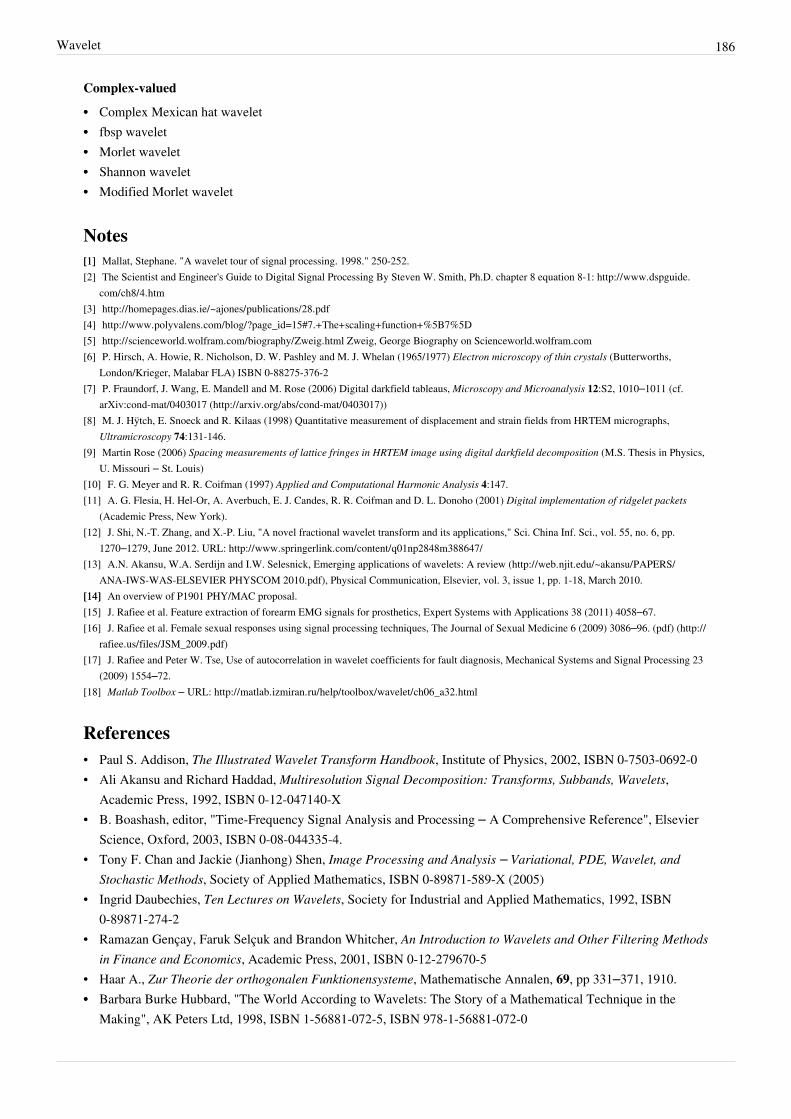
Wavelet 186
Complex-valued
•• Complex Mexican hat wavelet•• fbsp wavelet•• Morlet wavelet•• Shannon wavelet•• Modified Morlet wavelet
Notes[1][1] Mallat, Stephane. "A wavelet tour of signal processing. 1998." 250-252.[2] The Scientist and Engineer's Guide to Digital Signal Processing By Steven W. Smith, Ph.D. chapter 8 equation 8-1: http:/ / www. dspguide.
com/ ch8/ 4. htm[3] http:/ / homepages. dias. ie/ ~ajones/ publications/ 28. pdf[4] http:/ / www. polyvalens. com/ blog/ ?page_id=15#7. + The+ scaling+ function+ %5B7%5D[5] http:/ / scienceworld. wolfram. com/ biography/ Zweig. html Zweig, George Biography on Scienceworld.wolfram.com[6] P. Hirsch, A. Howie, R. Nicholson, D. W. Pashley and M. J. Whelan (1965/1977) Electron microscopy of thin crystals (Butterworths,
London/Krieger, Malabar FLA) ISBN 0-88275-376-2[7] P. Fraundorf, J. Wang, E. Mandell and M. Rose (2006) Digital darkfield tableaus, Microscopy and Microanalysis 12:S2, 1010–1011 (cf.
arXiv:cond-mat/0403017 (http:/ / arxiv. org/ abs/ cond-mat/ 0403017))[8] M. J. Hÿtch, E. Snoeck and R. Kilaas (1998) Quantitative measurement of displacement and strain fields from HRTEM micrographs,
Ultramicroscopy 74:131-146.[9] Martin Rose (2006) Spacing measurements of lattice fringes in HRTEM image using digital darkfield decomposition (M.S. Thesis in Physics,
U. Missouri – St. Louis)[10] F. G. Meyer and R. R. Coifman (1997) Applied and Computational Harmonic Analysis 4:147.[11] A. G. Flesia, H. Hel-Or, A. Averbuch, E. J. Candes, R. R. Coifman and D. L. Donoho (2001) Digital implementation of ridgelet packets
(Academic Press, New York).[12] J. Shi, N.-T. Zhang, and X.-P. Liu, "A novel fractional wavelet transform and its applications," Sci. China Inf. Sci., vol. 55, no. 6, pp.
1270–1279, June 2012. URL: http:/ / www. springerlink. com/ content/ q01np2848m388647/[13] A.N. Akansu, W.A. Serdijn and I.W. Selesnick, Emerging applications of wavelets: A review (http:/ / web. njit. edu/ ~akansu/ PAPERS/
ANA-IWS-WAS-ELSEVIER PHYSCOM 2010. pdf), Physical Communication, Elsevier, vol. 3, issue 1, pp. 1-18, March 2010.[14][14] An overview of P1901 PHY/MAC proposal.[15] J. Rafiee et al. Feature extraction of forearm EMG signals for prosthetics, Expert Systems with Applications 38 (2011) 4058–67.[16] J. Rafiee et al. Female sexual responses using signal processing techniques, The Journal of Sexual Medicine 6 (2009) 3086–96. (pdf) (http:/ /
rafiee. us/ files/ JSM_2009. pdf)[17] J. Rafiee and Peter W. Tse, Use of autocorrelation in wavelet coefficients for fault diagnosis, Mechanical Systems and Signal Processing 23
(2009) 1554–72.[18] Matlab Toolbox – URL: http:/ / matlab. izmiran. ru/ help/ toolbox/ wavelet/ ch06_a32. html
References• Paul S. Addison, The Illustrated Wavelet Transform Handbook, Institute of Physics, 2002, ISBN 0-7503-0692-0• Ali Akansu and Richard Haddad, Multiresolution Signal Decomposition: Transforms, Subbands, Wavelets,
Academic Press, 1992, ISBN 0-12-047140-X• B. Boashash, editor, "Time-Frequency Signal Analysis and Processing – A Comprehensive Reference", Elsevier
Science, Oxford, 2003, ISBN 0-08-044335-4.• Tony F. Chan and Jackie (Jianhong) Shen, Image Processing and Analysis – Variational, PDE, Wavelet, and
Stochastic Methods, Society of Applied Mathematics, ISBN 0-89871-589-X (2005)• Ingrid Daubechies, Ten Lectures on Wavelets, Society for Industrial and Applied Mathematics, 1992, ISBN
0-89871-274-2• Ramazan Gençay, Faruk Selçuk and Brandon Whitcher, An Introduction to Wavelets and Other Filtering Methods
in Finance and Economics, Academic Press, 2001, ISBN 0-12-279670-5• Haar A., Zur Theorie der orthogonalen Funktionensysteme, Mathematische Annalen, 69, pp 331–371, 1910.•• Barbara Burke Hubbard, "The World According to Wavelets: The Story of a Mathematical Technique in the
Making", AK Peters Ltd, 1998, ISBN 1-56881-072-5, ISBN 978-1-56881-072-0

Wavelet 187
• Gerald Kaiser, A Friendly Guide to Wavelets, Birkhauser, 1994, ISBN 0-8176-3711-7• Stéphane Mallat, "A wavelet tour of signal processing" 2nd Edition, Academic Press, 1999, ISBN 0-12-466606-X• Donald B. Percival and Andrew T. Walden, Wavelet Methods for Time Series Analysis, Cambridge University
Press, 2000, ISBN 0-521-68508-7• Press, WH; Teukolsky, SA; Vetterling, WT; Flannery, BP (2007), "Section 13.10. Wavelet Transforms" (http:/ /
apps. nrbook. com/ empanel/ index. html#pg=699), Numerical Recipes: The Art of Scientific Computing (3rd ed.),New York: Cambridge University Press, ISBN 978-0-521-88068-8
• P. P. Vaidyanathan, Multirate Systems and Filter Banks, Prentice Hall, 1993, ISBN 0-13-605718-7• Mladen Victor Wickerhauser, Adapted Wavelet Analysis From Theory to Software, A K Peters Ltd, 1994, ISBN
1-56881-041-5•• Martin Vetterli and Jelena Kovačević, "Wavelets and Subband Coding", Prentice Hall, 1995, ISBN
0-13-097080-8
External links• Hazewinkel, Michiel, ed. (2001), "Wavelet analysis" (http:/ / www. encyclopediaofmath. org/ index. php?title=p/
w097160), Encyclopedia of Mathematics, Springer, ISBN 978-1-55608-010-4• OpenSource Wavelet C# Code (http:/ / www. waveletstudio. net/ )• JWave – Open source Java implementation of several orthogonal and non-orthogonal wavelets (https:/ / code.
google. com/ p/ jwave/ )• Wavelet Analysis in Mathematica (http:/ / reference. wolfram. com/ mathematica/ guide/ Wavelets. html) (A very
comprehensive set of wavelet analysis tools)• 1st NJIT Symposium on Wavelets (April 30, 1990) (First Wavelets Conference in USA) (http:/ / web. njit. edu/
~ali/ s1. htm)• Binomial-QMF Daubechies Wavelets (http:/ / web. njit. edu/ ~ali/ NJITSYMP1990/
AkansuNJIT1STWAVELETSSYMPAPRIL301990. pdf)• Wavelets (http:/ / www-math. mit. edu/ ~gs/ papers/ amsci. pdf) by Gilbert Strang, American Scientist 82 (1994)
250–255. (A very short and excellent introduction)• Wavelet Digest (http:/ / www. wavelet. org)• NASA Signal Processor featuring Wavelet methods (http:/ / www. grc. nasa. gov/ WWW/ OptInstr/
NDE_Wave_Image_ProcessorLab. html) Description of NASA Signal & Image Processing Software and Link toDownload
• Course on Wavelets given at UC Santa Barbara, 2004 (http:/ / wavelets. ens. fr/ ENSEIGNEMENT/ COURS/UCSB/ index. html)
• The Wavelet Tutorial by Polikar (http:/ / users. rowan. edu/ ~polikar/ WAVELETS/ WTtutorial. html) (Easy tounderstand when you have some background with fourier transforms!)
• OpenSource Wavelet C++ Code (http:/ / herbert. the-little-red-haired-girl. org/ en/ software/ wavelet/ )• Wavelets for Kids (PDF file) (http:/ / www. isye. gatech. edu/ ~brani/ wp/ kidsA. pdf) (Introductory (for very
smart kids!))• Link collection about wavelets (http:/ / www. cosy. sbg. ac. at/ ~uhl/ wav. html)• Gerald Kaiser's acoustic and electromagnetic wavelets (http:/ / wavelets. com/ pages/ center. html)• A really friendly guide to wavelets (http:/ / perso. wanadoo. fr/ polyvalens/ clemens/ wavelets/ wavelets. html)• Wavelet-based image annotation and retrieval (http:/ / www. alipr. com)• Very basic explanation of Wavelets and how FFT relates to it (http:/ / www. relisoft. com/ Science/ Physics/
sampling. html)• A Practical Guide to Wavelet Analysis (http:/ / paos. colorado. edu/ research/ wavelets/ ) is very helpful, and the
wavelet software in FORTRAN, IDL and MATLAB are freely available online. Note that the biased waveletpower spectrum needs to be rectified (http:/ / ocgweb. marine. usf. edu/ ~liu/ wavelet. html).
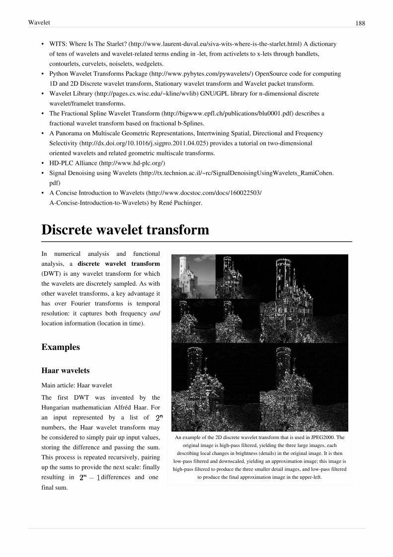
Wavelet 188
• WITS: Where Is The Starlet? (http:/ / www. laurent-duval. eu/ siva-wits-where-is-the-starlet. html) A dictionaryof tens of wavelets and wavelet-related terms ending in -let, from activelets to x-lets through bandlets,contourlets, curvelets, noiselets, wedgelets.
• Python Wavelet Transforms Package (http:/ / www. pybytes. com/ pywavelets/ ) OpenSource code for computing1D and 2D Discrete wavelet transform, Stationary wavelet transform and Wavelet packet transform.
• Wavelet Library (http:/ / pages. cs. wisc. edu/ ~kline/ wvlib) GNU/GPL library for n-dimensional discretewavelet/framelet transforms.
• The Fractional Spline Wavelet Transform (http:/ / bigwww. epfl. ch/ publications/ blu0001. pdf) describes afractional wavelet transform based on fractional b-Splines.
• A Panorama on Multiscale Geometric Representations, Intertwining Spatial, Directional and FrequencySelectivity (http:/ / dx. doi. org/ 10. 1016/ j. sigpro. 2011. 04. 025) provides a tutorial on two-dimensionaloriented wavelets and related geometric multiscale transforms.
• HD-PLC Alliance (http:/ / www. hd-plc. org/ )• Signal Denoising using Wavelets (http:/ / tx. technion. ac. il/ ~rc/ SignalDenoisingUsingWavelets_RamiCohen.
pdf)• A Concise Introduction to Wavelets (http:/ / www. docstoc. com/ docs/ 160022503/
A-Concise-Introduction-to-Wavelets) by René Puchinger.
Discrete wavelet transform
An example of the 2D discrete wavelet transform that is used in JPEG2000. Theoriginal image is high-pass filtered, yielding the three large images, each
describing local changes in brightness (details) in the original image. It is thenlow-pass filtered and downscaled, yielding an approximation image; this image ishigh-pass filtered to produce the three smaller detail images, and low-pass filtered
to produce the final approximation image in the upper-left.
In numerical analysis and functionalanalysis, a discrete wavelet transform(DWT) is any wavelet transform for whichthe wavelets are discretely sampled. As withother wavelet transforms, a key advantage ithas over Fourier transforms is temporalresolution: it captures both frequency andlocation information (location in time).
Examples
Haar wavelets
Main article: Haar waveletThe first DWT was invented by theHungarian mathematician Alfréd Haar. Foran input represented by a list of numbers, the Haar wavelet transform maybe considered to simply pair up input values,storing the difference and passing the sum.This process is repeated recursively, pairingup the sums to provide the next scale: finallyresulting in differences and onefinal sum.
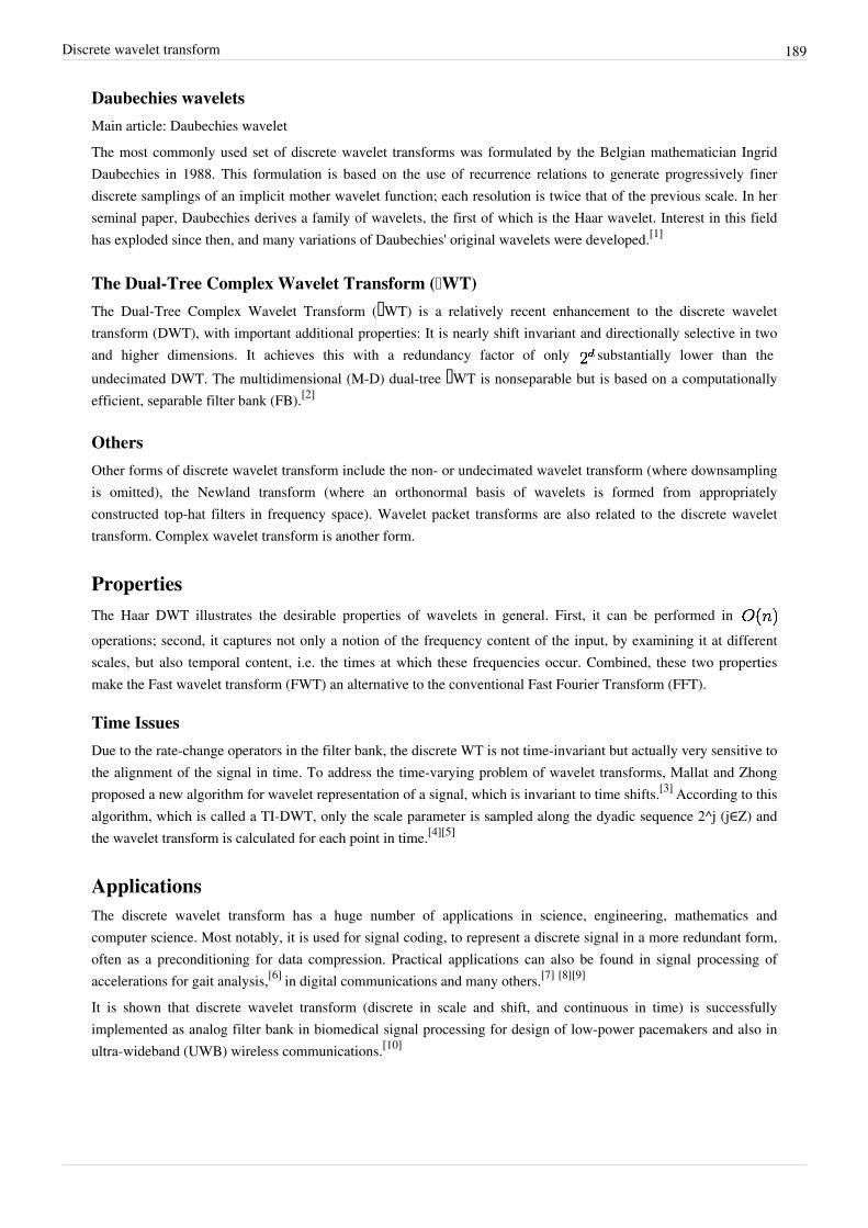
Discrete wavelet transform 189
Daubechies waveletsMain article: Daubechies waveletThe most commonly used set of discrete wavelet transforms was formulated by the Belgian mathematician IngridDaubechies in 1988. This formulation is based on the use of recurrence relations to generate progressively finerdiscrete samplings of an implicit mother wavelet function; each resolution is twice that of the previous scale. In herseminal paper, Daubechies derives a family of wavelets, the first of which is the Haar wavelet. Interest in this fieldhas exploded since then, and many variations of Daubechies' original wavelets were developed.[1]
The Dual-Tree Complex Wavelet Transform (ℂWT)The Dual-Tree Complex Wavelet Transform (ℂWT) is a relatively recent enhancement to the discrete wavelettransform (DWT), with important additional properties: It is nearly shift invariant and directionally selective in twoand higher dimensions. It achieves this with a redundancy factor of only substantially lower than theundecimated DWT. The multidimensional (M-D) dual-tree ℂWT is nonseparable but is based on a computationallyefficient, separable filter bank (FB).[2]
OthersOther forms of discrete wavelet transform include the non- or undecimated wavelet transform (where downsamplingis omitted), the Newland transform (where an orthonormal basis of wavelets is formed from appropriatelyconstructed top-hat filters in frequency space). Wavelet packet transforms are also related to the discrete wavelettransform. Complex wavelet transform is another form.
PropertiesThe Haar DWT illustrates the desirable properties of wavelets in general. First, it can be performed in operations; second, it captures not only a notion of the frequency content of the input, by examining it at differentscales, but also temporal content, i.e. the times at which these frequencies occur. Combined, these two propertiesmake the Fast wavelet transform (FWT) an alternative to the conventional Fast Fourier Transform (FFT).
Time IssuesDue to the rate-change operators in the filter bank, the discrete WT is not time-invariant but actually very sensitive tothe alignment of the signal in time. To address the time-varying problem of wavelet transforms, Mallat and Zhongproposed a new algorithm for wavelet representation of a signal, which is invariant to time shifts.[3] According to thisalgorithm, which is called a TI-DWT, only the scale parameter is sampled along the dyadic sequence 2^j (j∈Z) andthe wavelet transform is calculated for each point in time.[4][5]
ApplicationsThe discrete wavelet transform has a huge number of applications in science, engineering, mathematics andcomputer science. Most notably, it is used for signal coding, to represent a discrete signal in a more redundant form,often as a preconditioning for data compression. Practical applications can also be found in signal processing ofaccelerations for gait analysis,[6] in digital communications and many others.[7] [8][9]
It is shown that discrete wavelet transform (discrete in scale and shift, and continuous in time) is successfullyimplemented as analog filter bank in biomedical signal processing for design of low-power pacemakers and also inultra-wideband (UWB) wireless communications.[10]

Discrete wavelet transform 190
Comparison with Fourier transformSee also: Discrete Fourier transformTo illustrate the differences and similarities between the discrete wavelet transform with the discrete Fouriertransform, consider the DWT and DFT of the following sequence: (1,0,0,0), a unit impulse.The DFT has orthogonal basis (DFT matrix):
while the DWT with Haar wavelets for length 4 data has orthogonal basis in the rows of:
(To simplify notation, whole numbers are used, so the bases are orthogonal but not orthonormal.)Preliminary observations include:• Wavelets have location – the (1,1,–1,–1) wavelet corresponds to “left side” versus “right side”, while the last two
wavelets have support on the left side or the right side, and one is a translation of the other.• Sinusoidal waves do not have location – they spread across the whole space – but do have phase – the second and
third waves are translations of each other, corresponding to being 90° out of phase, like cosine and sine, of whichthese are discrete versions.
Decomposing the sequence with respect to these bases yields:
The DWT demonstrates the localization: the (1,1,1,1) term gives the average signal value, the (1,1,–1,–1) places thesignal in the left side of the domain, and the (1,–1,0,0) places it at the left side of the left side, and truncating at anystage yields a downsampled version of the signal:

Discrete wavelet transform 191
The sinc function, showing the time domainartifacts (undershoot and ringing) of truncating a
Fourier series.
The DFT, by contrast, expresses the sequence by the interference ofwaves of various frequencies – thus truncating the series yields alow-pass filtered version of the series:
Notably, the middle approximation (2-term) differs. From the frequency domain perspective, this is a betterapproximation, but from the time domain perspective it has drawbacks – it exhibits undershoot – one of the values isnegative, though the original series is non-negative everywhere – and ringing, where the right side is non-zero,unlike in the wavelet transform. On the other hand, the Fourier approximation correctly shows a peak, and all pointsare within of their correct value, though all points have error. The wavelet approximation, by contrast, places apeak on the left half, but has no peak at the first point, and while it is exactly correct for half the values (reflectinglocation), it has an error of for the other values.This illustrates the kinds of trade-offs between these transforms, and how in some respects the DWT providespreferable behavior, particularly for the modeling of transients.
Definition
One level of the transformThe DWT of a signal is calculated by passing it through a series of filters. First the samples are passed through alow pass filter with impulse response resulting in a convolution of the two:
The signal is also decomposed simultaneously using a high-pass filter . The outputs giving the detail coefficients(from the high-pass filter) and approximation coefficients (from the low-pass). It is important that the two filters arerelated to each other and they are known as a quadrature mirror filter.However, since half the frequencies of the signal have now been removed, half the samples can be discardedaccording to Nyquist’s rule. The filter outputs are then subsampled by 2 (Mallat's and the common notation is theopposite, g- high pass and h- low pass):
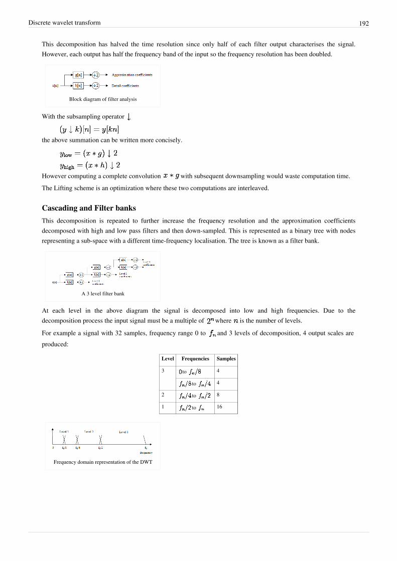
Discrete wavelet transform 192
This decomposition has halved the time resolution since only half of each filter output characterises the signal.However, each output has half the frequency band of the input so the frequency resolution has been doubled.
Block diagram of filter analysis
With the subsampling operator
the above summation can be written more concisely.
However computing a complete convolution with subsequent downsampling would waste computation time.The Lifting scheme is an optimization where these two computations are interleaved.
Cascading and Filter banksThis decomposition is repeated to further increase the frequency resolution and the approximation coefficientsdecomposed with high and low pass filters and then down-sampled. This is represented as a binary tree with nodesrepresenting a sub-space with a different time-frequency localisation. The tree is known as a filter bank.
A 3 level filter bank
At each level in the above diagram the signal is decomposed into low and high frequencies. Due to thedecomposition process the input signal must be a multiple of where is the number of levels.
For example a signal with 32 samples, frequency range 0 to and 3 levels of decomposition, 4 output scales areproduced:
Level Frequencies Samples
3 to 4
to 4
2 to 8
1 to 16
Frequency domain representation of the DWT
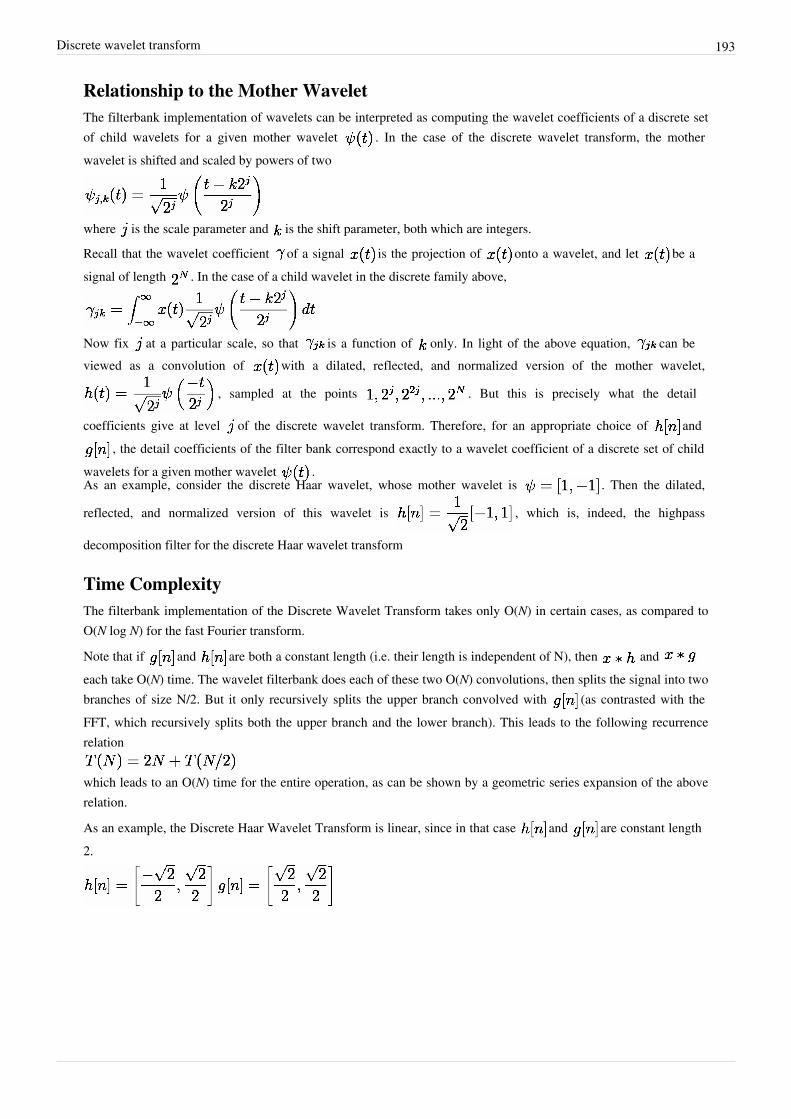
Discrete wavelet transform 193
Relationship to the Mother WaveletThe filterbank implementation of wavelets can be interpreted as computing the wavelet coefficients of a discrete setof child wavelets for a given mother wavelet . In the case of the discrete wavelet transform, the motherwavelet is shifted and scaled by powers of two
where is the scale parameter and is the shift parameter, both which are integers.
Recall that the wavelet coefficient of a signal is the projection of onto a wavelet, and let be asignal of length . In the case of a child wavelet in the discrete family above,
Now fix at a particular scale, so that is a function of only. In light of the above equation, can beviewed as a convolution of with a dilated, reflected, and normalized version of the mother wavelet,
, sampled at the points . But this is precisely what the detail
coefficients give at level of the discrete wavelet transform. Therefore, for an appropriate choice of and, the detail coefficients of the filter bank correspond exactly to a wavelet coefficient of a discrete set of child
wavelets for a given mother wavelet .As an example, consider the discrete Haar wavelet, whose mother wavelet is . Then the dilated,
reflected, and normalized version of this wavelet is , which is, indeed, the highpass
decomposition filter for the discrete Haar wavelet transform
Time ComplexityThe filterbank implementation of the Discrete Wavelet Transform takes only O(N) in certain cases, as compared toO(N log N) for the fast Fourier transform.
Note that if and are both a constant length (i.e. their length is independent of N), then and each take O(N) time. The wavelet filterbank does each of these two O(N) convolutions, then splits the signal into twobranches of size N/2. But it only recursively splits the upper branch convolved with (as contrasted with theFFT, which recursively splits both the upper branch and the lower branch). This leads to the following recurrencerelation
which leads to an O(N) time for the entire operation, as can be shown by a geometric series expansion of the aboverelation.
As an example, the Discrete Haar Wavelet Transform is linear, since in that case and are constant length2.

Discrete wavelet transform 194
Other transformsSee also: Adam7 algorithmThe Adam7 algorithm, used for interlacing in the Portable Network Graphics (PNG) format, is a multiscale model ofthe data which is similar to a DWT with Haar wavelets.Unlike the DWT, it has a specific scale – it starts from an 8×8 block, and it downsamples the image, rather thandecimating (low-pass filtering, then downsampling). It thus offers worse frequency behavior, showing artifacts(pixelation) at the early stages, in return for simpler implementation.
Code exampleIn its simplest form, the DWT is remarkably easy to compute.The Haar wavelet in Java:
public static int[] discreteHaarWaveletTransform(int[] input) {
// This function assumes that input.length=2^n, n>1
int[] output = new int[input.length];
for (int length = input.length >> 1; ; length >>= 1) {
// length = input.length / 2^n, WITH n INCREASING to
log(input.length) / log(2)
for (int i = 0; i < length; ++i) {
int sum = input[i * 2] + input[i * 2 + 1];
int difference = input[i * 2] - input[i * 2 + 1];
output[i] = sum;
output[length + i] = difference;
}
if (length == 1) {
return output;
}
//Swap arrays to do next iteration
System.arraycopy(output, 0, input, 0, length << 1);
}
}
Complete Java code for a 1-D and 2-D DWT using Haar, Daubechies, Coiflet, and Legendre wavelets is availablefrom the open source project: JWave [11]. Furthermore, a fast lifting implementation of the discrete biorthogonalCDF 9/7 wavelet transform in C, used in the JPEG 2000 image compression standard can be found here [12]
(archived 5th March 2012).
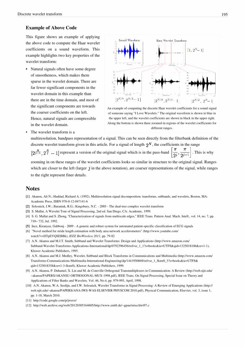
Discrete wavelet transform 195
Example of Above Code
An example of computing the discrete Haar wavelet coefficients for a sound signalof someone saying "I Love Wavelets." The original waveform is shown in blue inthe upper left, and the wavelet coefficients are shown in black in the upper right.
Along the bottom is shown three zoomed-in regions of the wavelet coefficients fordifferent ranges.
This figure shows an example of applyingthe above code to compute the Haar waveletcoefficients on a sound waveform. Thisexample highlights two key properties of thewavelet transform:•• Natural signals often have some degree
of smootheness, which makes themsparse in the wavelet domain. There arefar fewer significant components in thewavelet domain in this example thanthere are in the time domain, and most ofthe significant components are towardsthe coarser coefficients on the left.Hence, natural signals are compressiblein the wavelet domain.
• The wavelet transform is amultiresolution, bandpass representation of a signal. This can be seen directly from the filterbank definition of thediscrete wavelet transform given in this article. For a signal of length , the coefficients in the range
represent a version of the original signal which is in the pass-band . This is why
zooming in on these ranges of the wavelet coefficients looks so similar in structure to the original signal. Rangeswhich are closer to the left (larger in the above notation), are coarser representations of the signal, while rangesto the right represent finer details.
Notes[1][1] Akansu, Ali N.; Haddad, Richard A. (1992), Multiresolution signal decomposition: transforms, subbands, and wavelets, Boston, MA:
Academic Press, ISBN 978-0-12-047141-6[2][2] Selesnick, I.W.; Baraniuk, R.G.; Kingsbury, N.C. - 2005 - The dual-tree complex wavelet transform[3][3] S. Mallat, A Wavelet Tour of Signal Processing, 2nd ed. San Diego, CA: Academic, 1999.[4] S. G. Mallat and S. Zhong, “Characterization of signals from multiscale edges,” IEEE Trans. Pattern Anal. Mach. Intell., vol. 14, no. 7, pp.
710– 732, Jul. 1992.[5][5] Ince, Kiranyaz, Gabbouj - 2009 - A generic and robust system for automated patient-specific classification of ECG signals[6] "Novel method for stride length estimation with body area network accelerometers" (http:/ / www. youtube. com/
watch?v=DTpEVQSEBBk), IEEE BioWireless 2011, pp. 79-82[7] A.N. Akansu and M.J.T. Smith, Subband and Wavelet Transforms: Design and Applications (http:/ / www. amazon. com/
Subband-Wavelet-Transforms-Applications-International/ dp/ 0792396456/ ref=sr_1_1?s=books& ie=UTF8& qid=1325018106& sr=1-1),Kluwer Academic Publishers, 1995.
[8] A.N. Akansu and M.J. Medley, Wavelet, Subband and Block Transforms in Communications and Multimedia (http:/ / www. amazon. com/Transforms-Communications-Multimedia-International-Engineering/ dp/ 1441950869/ ref=sr_1_fkmr0_3?s=books& ie=UTF8&qid=1325018358& sr=1-3-fkmr0), Kluwer Academic Publishers, 1999.
[9] A.N. Akansu, P. Duhamel, X. Lin and M. de Courville Orthogonal Transmultiplexers in Communication: A Review (http:/ / web. njit. edu/~akansu/ PAPERS/ AKANSU-ORTHOGONAL-MUX-1998. pdf), IEEE Trans. On Signal Processing, Special Issue on Theory andApplications of Filter Banks and Wavelets. Vol. 46, No.4, pp. 979-995, April, 1998.
[10] A.N. Akansu, W.A. Serdijn, and I.W. Selesnick, Wavelet Transforms in Signal Processing: A Review of Emerging Applications (http:/ /web. njit. edu/ ~akansu/ PAPERS/ ANA-IWS-WAS-ELSEVIER PHYSCOM 2010. pdf), Physical Communication, Elsevier, vol. 3, issue 1,pp. 1-18, March 2010.
[11] http:/ / code. google. com/ p/ jwave/[12] http:/ / web. archive. org/ web/ 20120305164605/ http:/ / www. embl. de/ ~gpau/ misc/ dwt97. c

Discrete wavelet transform 196
References
Fast wavelet transformThe Fast Wavelet Transform is a mathematical algorithm designed to turn a waveform or signal in the time domaininto a sequence of coefficients based on an orthogonal basis of small finite waves, or wavelets. The transform can beeasily extended to multidimensional signals, such as images, where the time domain is replaced with the spacedomain.It has as theoretical foundation the device of a finitely generated, orthogonal multiresolution analysis (MRA). In theterms given there, one selects a sampling scale J with sampling rate of 2J per unit interval, and projects the givensignal f onto the space ; in theory by computing the scalar products
where is the scaling function of the chosen wavelet transform; in practice by any suitable sampling procedureunder the condition that the signal is highly oversampled, so
is the orthogonal projection or at least some good approximation of the original signal in .The MRA is characterised by its scaling sequence
or, as Z-transform,
and its wavelet sequence
or
(some coefficients might be zero). Those allow to compute the wavelet coefficients , at least some rangek=M,...,J-1, without having to approximate the integrals in the corresponding scalar products. Instead, one candirectly, with the help of convolution and decimation operators, compute those coefficients from the firstapproximation .
Forward DWTOne computes recursively, starting with the coefficient sequence and counting down from k=J-1 to some M<J,
single application of a wavelet filter bank, with filters g=a*, h=b*
or
and
or
,for k=J-1,J-2,...,M and all . In the Z-transform notation:

Fast wavelet transform 197
recursive application of the filter bank
• The downsampling operatorreduces an infinite
sequence, given by itsZ-transform, which is simply aLaurent series, to the sequence ofthe coefficients with evenindices,
.
• The starred Laurent-polynomial denotes the adjoint filter, it has time-reversed adjoint coefficients,
. (The adjoint of a real number being the number itself, of a complex number its
conjugate, of a real matrix the transposed matrix, of a complex matrix its hermitian adjoint).•• Multiplication is polynomial multiplication, which is equivalent to the convolution of the coefficient
sequences.It follows that
is the orthogonal projection of the original signal f or at least of the first approximation onto the subspace, that is, with sampling rate of 2k per unit interval. The difference to the first approximation is given by
,where the difference or detail signals are computed from the detail coefficients as
,
with denoting the mother wavelet of the wavelet transform.
Inverse DWTGiven the coefficient sequence for some M<J and all the difference sequences , k=M,...,J-1, onecomputes recursively
or
for k=J-1,J-2,...,M and all . In the Z-transform notation:
• The upsampling operator creates zero-filled holes inside a given sequence. That is, every secondelement of the resulting sequence is an element of the given sequence, every other second element is zero or
. This linear operator is, in the Hilbert space , the adjoint to the
downsampling operator .

Fast wavelet transform 198
References• A.N. Akansu Multiplierless Suboptimal PR-QMF Design Proc. SPIE 1818, Visual Communications and Image
Processing, p. 723, November, 1992• A.N. Akansu Multiplierless 2-band Perfect Reconstruction Quadrature Mirror Filter (PR-QMF) Banks US Patent
5,420,891, 1995• A.N. Akansu Multiplierless PR Quadrature Mirror Filters for Subband Image Coding IEEE Trans. Image
Processing, p. 1359, September 1996• M.J. Mohlenkamp, M.C. Pereyra Wavelets, Their Friends, and What They Can Do for You (2008 EMS) p. 38• B.B. Hubbard The World According to Wavelets: The Story of a Mathematical Technique in the Making (1998
Peters) p. 184• S.G. Mallat A Wavelet Tour of Signal Processing (1999 Academic Press) p. 255• A. Teolis Computational Signal Processing with Wavelets (1998 Birkhäuser) p. 116• Y. Nievergelt Wavelets Made Easy (1999 Springer) p. 95
Further readingG. Beylkin, R. Coifman, V. Rokhlin, "Fast wavelet transforms and numerical algorithms" Comm. Pure Appl. Math.,44 (1991) pp. 141–183
Haar wavelet
The Haar wavelet
In mathematics, the Haar wavelet is a sequence of rescaled"square-shaped" functions which together form a wavelet family orbasis. Wavelet analysis is similar to Fourier analysis in that it allows atarget function over an interval to be represented in terms of anorthonormal function basis. The Haar sequence is now recognised asthe first known wavelet basis and extensively used as a teachingexample.
The Haar sequence was proposed in 1909 by Alfréd Haar.[1] Haarused these functions to give an example of an orthonormal system forthe space of square-integrable functions on the unit interval [0, 1]. Thestudy of wavelets, and even the term "wavelet", did not come until much later. As a special case of the Daubechieswavelet, the Haar wavelet is also known as D2.
The Haar wavelet is also the simplest possible wavelet. The technical disadvantage of the Haar wavelet is that it isnot continuous, and therefore not differentiable. This property can, however, be an advantage for the analysis ofsignals with sudden transitions, such as monitoring of tool failure in machines.
The Haar wavelet's mother wavelet function can be described as
Its scaling function can be described as

Haar wavelet 199
Haar functions and Haar systemFor every pair n, k of integers in Z, the Haar function ψn, k is defined on the real line R by the formula
This function is supported on the right-open interval In, k = [ k 2−n, (k+1) 2−n ), i.e., it vanishes outside that interval. Ithas integral 0 and norm 1 in the Hilbert space L2(R),
The Haar functions are pairwise orthogonal,
where δi,j represents the Kronecker delta. Here is the reason for orthogonality: when the two supporting intervalsand are not equal, then they are either disjoint, or else, the smaller of the two supports, say , is
contained in the lower or in the upper half of the other interval, on which the function remains constant. Itfollows in this case that the product of these two Haar functions is a multiple of the first Haar function, hence theproduct has integral 0.The Haar system on the real line is the set of functions
It is complete in L2(R): The Haar system on the line is an orthonormal basis in L2(R).
Haar wavelet propertiesThe Haar wavelet has several notable properties:1. Any continuous real function with compact support can be approximated uniformly by linear combinations of
and their shifted functions. This extends to those function spaces whereany function therein can be approximated by continuous functions.
2. Any continuous real function on [0, 1] can be approximated uniformly on [0, 1] by linear combinations of theconstant function 1, and their shifted functions.[2]
3. Orthogonality in the form
Here δi,j represents the Kronecker delta. The dual function of ψ(t) is ψ(t) itself.1. Wavelet/scaling functions with different scale n have a functional relationship: since
it follows that coefficients of scale n can be calculated by coefficients of scale n+1:
If
and
then

Haar wavelet 200
Haar system on the unit interval and related systemsIn this section, the discussion is restricted to the unit interval [0, 1] and to the Haar functions that are supported on[0, 1]. The system of functions considered by Haar in 1910,[3] called the Haar system on [0, 1] in this article,consists of the subset of Haar wavelets defined as
with the addition of the constant function 1 on [0, 1].In Hilbert space terms, this Haar system on [0, 1] is a complete orthonormal system, i.e., an orthonormal basis, forthe space L2([0, 1]) of square integrable functions on the unit interval.The Haar system on [0, 1] —with the constant function 1 as first element, followed with the Haar functions orderedaccording to the lexicographic ordering of couples (n, k)— is further a monotone Schauder basis for the spaceLp([0, 1]) when 1 ≤ p < ∞.[4] This basis is unconditional when 1 < p < ∞.[5]
There is a related Rademacher system consisting of sums of Haar functions,
Notice that |rn(t)| = 1 on [0, 1). This is an orthonormal system but it is not complete. In the language of probabilitytheory, the Rademacher sequence is an instance of a sequence of independent Bernoulli random variables withmean 0. The Khintchine inequality expresses the fact that in all the spaces Lp([0, 1]), 1 ≤ p < ∞, the Rademachersequence is equivalent to the unit vector basis in ℓ2.[6] In particular, the closed linear span of the Rademachersequence in Lp([0, 1]), 1 ≤ p < ∞, is isomorphic to ℓ2.
The Faber–Schauder systemThe Faber–Schauder system[7][8] is the family of continuous functions on [0, 1] consisting of the constantfunction 1, and of multiples of indefinite integrals of the functions in the Haar system on [0, 1], chosen to havenorm 1 in the maximum norm. This system begins with s0 = 1, then s1(t) = t is the indefinite integral vanishing at 0of the function 1, first element of the Haar system on [0, 1]. Next, for every integer n ≥ 0, functions sn, k are definedby the formula
These functions sn, k are continuous, piecewise linear, supported by the interval In, k that also supports ψn, k. Thefunction sn, k is equal to 1 at the midpoint xn, k of the interval In, k, linear on both halves of that interval. It takesvalues between 0 and 1 everywhere.The Faber–Schauder system is a Schauder basis for the space C([0, 1]) of continuous functions on [0, 1]. For every fin C([0, 1]), the partial sum
of the series expansion of f in the Faber–Schauder system is the continuous piecewise linear function that agreeswith f at the 2n + 1 points k 2−n, where 0 ≤ k ≤ 2n. Next, the formula
gives a way to compute the expansion of f step by step. Since f is uniformly continuous, the sequence {fn} convergesuniformly to f. It follows that the Faber–Schauder series expansion of f converges in C([0, 1]), and the sum of thisseries is equal to f.
Haar wavelet 201
The Franklin systemThe Franklin system is obtained from the Faber–Schauder system by the Gram–Schmidt orthonormalizationprocedure.[9][10] Since the Franklin system has the same linear span as that of the Faber–Schauder system, this spanis dense in C([0, 1]), hence in L2([0, 1]). The Franklin system is therefore an orthonormal basis for L2([0, 1]),consisting of continuous piecewise linear functions. P. Franklin proved in 1928 that this system is a Schauder basisfor C([0, 1]).[11] The Franklin system is also an unconditional basis for the space Lp([0, 1]) when 1 < p < ∞.[12] TheFranklin system provides a Schauder basis in the disk algebra A(D). This was proved in 1974 by Bočkarev, after theexistence of a basis for the disk algebra had remained open for more than forty years.[13]
Bočkarev's construction of a Schauder basis in A(D) goes as follows: let f be a complex valued Lipschitz function on[0, π]; then f is the sum of a cosine series with absolutely summable coefficients. Let T(f) be the element of A(D)defined by the complex power series with the same coefficients,
Bočkarev's basis for A(D) is formed by the images under T of the functions in the Franklin system on [0, π].Bočkarev's equivalent description for the mapping T starts by extending f to an even Lipschitz function g1 on [−π, π],identified with a Lipschitz function on the unit circle T. Next, let g2 be the conjugate function of g1, and define T(f)to be the function in A(D) whose value on the boundary T of D is equal to g1 + i g2.When dealing with 1-periodic continuous functions, or rather with continuous functions f on [0, 1] such that f(0) =f(1), one removes the function s1(t) = t from the Faber–Schauder system, in order to obtain the periodicFaber–Schauder system. The periodic Franklin system is obtained by orthonormalization from the periodicFaber–-Schauder system.[14] One can prove Bočkarev's result on A(D) by proving that the periodic Franklin systemon [0, 2π] is a basis for a Banach space Ar isomorphic to A(D). The space Ar consists of complex continuousfunctions on the unit circle T whose conjugate function is also continuous.
Haar matrixThe 2×2 Haar matrix that is associated with the Haar wavelet is
Using the discrete wavelet transform, one can transform any sequence of even lengthinto a sequence of two-component-vectors . If one right-multiplies each vector withthe matrix , one gets the result of one stage of the fast Haar-wavelet transform.Usually one separates the sequences s and d and continues with transforming the sequence s. Sequence s is oftenreferred to as the averages part, whereas d is known as the details part.If one has a sequence of length a multiple of four, one can build blocks of 4 elements and transform them in a similarmanner with the 4×4 Haar matrix
which combines two stages of the fast Haar-wavelet transform.Compare with a Walsh matrix, which is a non-localized 1/–1 matrix.Generally, the 2N×2N Haar matrix can be derived by the following equation.

Haar wavelet 202
where and is the Kronecker product.
The Kronecker product of , where is an m×n matrix and is a p×q matrix, is expressed as
An un-normalized 8-point Haar matrix is shown below
Note that, the above matrix is an un-normalized Haar matrix. The Haar matrix required by the Haar transform shouldbe normalized.From the definition of the Haar matrix , one can observe that, unlike the Fourier transform, matrix has onlyreal elements (i.e., 1, -1 or 0) and is non-symmetric.Take 8-point Haar matrix as an example. The first row of matrix measures the average value, and thesecond row matrix measures a low frequency component of the input vector. The next two rows are sensitive tothe first and second half of the input vector respectively, which corresponds to moderate frequency components. Theremaining four rows are sensitive to the four section of the input vector, which corresponds to high frequencycomponents.
Haar transformThe Haar transform is the simplest of the wavelet transforms. This transform cross-multiplies a function against theHaar wavelet with various shifts and stretches, like the Fourier transform cross-multiplies a function against a sinewave with two phases and many stretches.[15]
IntroductionThe Haar transform is one of the oldest transform functions, proposed in 1910 by a Hungarian mathematicianAlfred Haar. It is found effective in applications such as signal and image compression in electrical and computerengineering as it provides a simple and computationally efficient approach for analysing the local aspects of a signal.The Haar transform is derived from the Haar matrix. An example of a 4x4 Haar transformation matrix is shownbelow.
The Haar transform can be thought of as a sampling process in which rows of the transformation matrix act assamples of finer and finer resolution.
Haar wavelet 203
Compare with the Walsh transform, which is also 1/–1, but is non-localized.
PropertyThe Haar transform has the following properties
1. No need for multiplications. It requires only additions and there are many elements with zero value in theHaar matrix, so the computation time is short. It is faster than Walsh transform, whose matrix is composed of+1 and -1.2. Input and output length are the same. However, the length should be a power of 2, i.e. .3. It can be used to analyse the localized feature of signals. Due to the orthogonal property of Haar function,the frequency components of input signal can be analyzed.
Haar transform and Inverse Haar transformThe Haar transform yn of an n-input function xn is
The Haar transform matrix is real and orthogonal. Thus, the inverse Haar transform can be derived by the followingequations.
where is the identity matrix. For example, when n = 4
Thus, the inverse Haar transform is
Example
The Haar transform coefficients of a n=4-point signal can be found as
The input signal can reconstruct by the inverse Haar transform
ApplicationModern cameras are capable of producing images with resolutions in the range of tens of megapixels. These imagesneed to be compressed before storage and transfer. The Haar transform can be used for image compression. Thebasic idea is to transfer the image into a matrix in which each element of the matrix represents a pixel in the image.For example, a 256×256 matrix is saved for a 256×256 image. JPEG image compression involves cutting the originalimage into 8×8 sub-images. Each sub-image is an 8×8 matrix.
Haar wavelet 204
The 2-D Haar transform is required. The equation of the Haar transform is , where is a n×nmatrix and is n-point Haar transform. The inverse Haar transform is
Notes[1][1] see p. 361 in .[2][2] As opposed to the preceding statement, this fact is not obvious: see p. 363 in .[3][3] p. 361 in[4] see p. 3 in J. Lindenstrauss, L. Tzafriri, (1977), "Classical Banach Spaces I, Sequence Spaces", Ergebnisse der Mathematik und ihrer
Grenzgebiete 92, Berlin: Springer-Verlag, ISBN 3-540-08072-4.[5] The result is due to R. E. Paley, A remarkable series of orthogonal functions (I), Proc. London Math. Soc. 34 (1931) pp. 241-264. See also
p. 155 in J. Lindenstrauss, L. Tzafriri, (1979), "Classical Banach spaces II, Function spaces". Ergebnisse der Mathematik und ihrerGrenzgebiete 97, Berlin: Springer-Verlag, ISBN 3-540-08888-1.
[6] see for example p. 66 in J. Lindenstrauss, L. Tzafriri, (1977), "Classical Banach Spaces I, Sequence Spaces", Ergebnisse der Mathematik undihrer Grenzgebiete 92, Berlin: Springer-Verlag, ISBN 3-540-08072-4.
[7] Faber, Georg (1910), "Über die Orthogonalfunktionen des Herrn Haar", Deutsche Math.-Ver (in German) 19: 104–112. ISSN 0012-0456;http:/ / www-gdz. sub. uni-goettingen. de/ cgi-bin/ digbib. cgi?PPN37721857X ; http:/ / resolver. sub. uni-goettingen. de/purl?GDZPPN002122553
[8] Schauder, Juliusz (1928), "Eine Eigenschaft des Haarschen Orthogonalsystems", Mathematische Zeitschrift 28: 317–320.[9] see Z. Ciesielski, Properties of the orthonormal Franklin system. Studia Math. 23 1963 141–157.[10] Franklin system. B.I. Golubov (originator), Encyclopedia of Mathematics. URL: http:/ / www. encyclopediaofmath. org/ index.
php?title=Franklin_system& oldid=16655[11] Philip Franklin, A set of continuous orthogonal functions, Math. Ann. 100 (1928), 522-529.[12] S. V. Bočkarev, Existence of a basis in the space of functions analytic in the disc, and some properties of Franklin's system. Mat. Sb. 95
(1974), 3–18 (Russian). Translated in Math. USSR-Sb. 24 (1974), 1–16.[13] The question appears p. 238, §3 in Banach's book, . The disk algebra A(D) appears as Example 10, p. 12 in Banach's book.[14][14] See p. 161, III.D.20 and p. 192, III.E.17 in[15] The Haar Transform (http:/ / sepwww. stanford. edu/ public/ docs/ sep75/ ray2/ paper_html/ node4. html)
References• Haar, Alfréd (1910), "Zur Theorie der orthogonalen Funktionensysteme", Mathematische Annalen 69 (3):
331–371, doi: 10.1007/BF01456326 (http:/ / dx. doi. org/ 10. 1007/ BF01456326)• Charles K. Chui, An Introduction to Wavelets, (1992), Academic Press, San Diego, ISBN 0-585-47090-1• English Translation of the seminal Haar's article: https:/ / www. uni-hohenheim. de/ ~gzim/ Publications/ haar.
External links• Hazewinkel, Michiel, ed. (2001), "Haar system" (http:/ / www. encyclopediaofmath. org/ index. php?title=p/
h046070), Encyclopedia of Mathematics, Springer, ISBN 978-1-55608-010-4• Free Haar wavelet filtering implementation and interactive demo (http:/ / www. tomgibara. com/ computer-vision/
haar-wavelet)• Free Haar wavelet denoising and lossy signal compression (http:/ / packages. debian. org/ wzip)
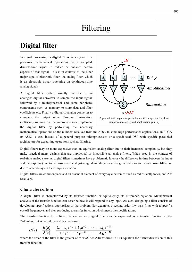
205
Filtering
Digital filter
A general finite impulse response filter with n stages, each with anindependent delay, di, and amplification gain, ai.
In signal processing, a digital filter is a system thatperforms mathematical operations on a sampled,discrete-time signal to reduce or enhance certainaspects of that signal. This is in contrast to the othermajor type of electronic filter, the analog filter, whichis an electronic circuit operating on continuous-timeanalog signals.
A digital filter system usually consists of ananalog-to-digital converter to sample the input signal,followed by a microprocessor and some peripheralcomponents such as memory to store data and filtercoefficients etc. Finally a digital-to-analog converter tocomplete the output stage. Program Instructions(software) running on the microprocessor implementthe digital filter by performing the necessarymathematical operations on the numbers received from the ADC. In some high performance applications, an FPGAor ASIC is used instead of a general purpose microprocessor, or a specialized DSP with specific paralleledarchitecture for expediting operations such as filtering.
Digital filters may be more expensive than an equivalent analog filter due to their increased complexity, but theymake practical many designs that are impractical or impossible as analog filters. When used in the context ofreal-time analog systems, digital filters sometimes have problematic latency (the difference in time between the inputand the response) due to the associated analog-to-digital and digital-to-analog conversions and anti-aliasing filters, ordue to other delays in their implementation.Digital filters are commonplace and an essential element of everyday electronics such as radios, cellphones, and AVreceivers.
CharacterizationA digital filter is characterized by its transfer function, or equivalently, its difference equation. Mathematicalanalysis of the transfer function can describe how it will respond to any input. As such, designing a filter consists ofdeveloping specifications appropriate to the problem (for example, a second-order low pass filter with a specificcut-off frequency), and then producing a transfer function which meets the specifications.The transfer function for a linear, time-invariant, digital filter can be expressed as a transfer function in theZ-domain; if it is causal, then it has the form:
where the order of the filter is the greater of N or M. See Z-transform's LCCD equation for further discussion of thistransfer function.
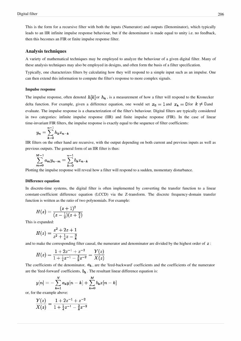
Digital filter 206
This is the form for a recursive filter with both the inputs (Numerator) and outputs (Denominator), which typicallyleads to an IIR infinite impulse response behaviour, but if the denominator is made equal to unity i.e. no feedback,then this becomes an FIR or finite impulse response filter.
Analysis techniquesA variety of mathematical techniques may be employed to analyze the behaviour of a given digital filter. Many ofthese analysis techniques may also be employed in designs, and often form the basis of a filter specification.Typically, one characterizes filters by calculating how they will respond to a simple input such as an impulse. Onecan then extend this information to compute the filter's response to more complex signals.
Impulse response
The impulse response, often denoted or , is a measurement of how a filter will respond to the Kroneckerdelta function. For example, given a difference equation, one would set and for andevaluate. The impulse response is a characterization of the filter's behaviour. Digital filters are typically consideredin two categories: infinite impulse response (IIR) and finite impulse response (FIR). In the case of lineartime-invariant FIR filters, the impulse response is exactly equal to the sequence of filter coefficients:
IIR filters on the other hand are recursive, with the output depending on both current and previous inputs as well asprevious outputs. The general form of an IIR filter is thus:
Plotting the impulse response will reveal how a filter will respond to a sudden, momentary disturbance.
Difference equation
In discrete-time systems, the digital filter is often implemented by converting the transfer function to a linearconstant-coefficient difference equation (LCCD) via the Z-transform. The discrete frequency-domain transferfunction is written as the ratio of two polynomials. For example:
This is expanded:
and to make the corresponding filter causal, the numerator and denominator are divided by the highest order of :
The coefficients of the denominator, , are the 'feed-backward' coefficients and the coefficients of the numeratorare the 'feed-forward' coefficients, . The resultant linear difference equation is:
or, for the example above:
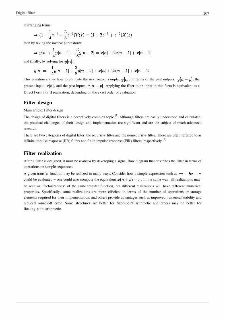
Digital filter 207
rearranging terms:
then by taking the inverse z-transform:
and finally, by solving for :
This equation shows how to compute the next output sample, , in terms of the past outputs, , thepresent input, , and the past inputs, . Applying the filter to an input in this form is equivalent to aDirect Form I or II realization, depending on the exact order of evaluation.
Filter designMain article: Filter designThe design of digital filters is a deceptively complex topic.[1] Although filters are easily understood and calculated,the practical challenges of their design and implementation are significant and are the subject of much advancedresearch.There are two categories of digital filter: the recursive filter and the nonrecursive filter. These are often referred to asinfinite impulse response (IIR) filters and finite impulse response (FIR) filters, respectively.[2]
Filter realizationAfter a filter is designed, it must be realized by developing a signal flow diagram that describes the filter in terms ofoperations on sample sequences.A given transfer function may be realized in many ways. Consider how a simple expression such as could be evaluated – one could also compute the equivalent . In the same way, all realizations maybe seen as "factorizations" of the same transfer function, but different realizations will have different numericalproperties. Specifically, some realizations are more efficient in terms of the number of operations or storageelements required for their implementation, and others provide advantages such as improved numerical stability andreduced round-off error. Some structures are better for fixed-point arithmetic and others may be better forfloating-point arithmetic.
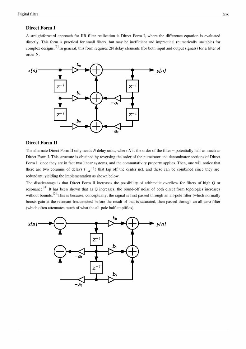
Digital filter 208
Direct Form IA straightforward approach for IIR filter realization is Direct Form I, where the difference equation is evaluateddirectly. This form is practical for small filters, but may be inefficient and impractical (numerically unstable) forcomplex designs.[3] In general, this form requires 2N delay elements (for both input and output signals) for a filter oforder N.
Direct Form IIThe alternate Direct Form II only needs N delay units, where N is the order of the filter – potentially half as much asDirect Form I. This structure is obtained by reversing the order of the numerator and denominator sections of DirectForm I, since they are in fact two linear systems, and the commutativity property applies. Then, one will notice thatthere are two columns of delays ( ) that tap off the center net, and these can be combined since they areredundant, yielding the implementation as shown below.The disadvantage is that Direct Form II increases the possibility of arithmetic overflow for filters of high Q orresonance.[4] It has been shown that as Q increases, the round-off noise of both direct form topologies increaseswithout bounds.[5] This is because, conceptually, the signal is first passed through an all-pole filter (which normallyboosts gain at the resonant frequencies) before the result of that is saturated, then passed through an all-zero filter(which often attenuates much of what the all-pole half amplifies).
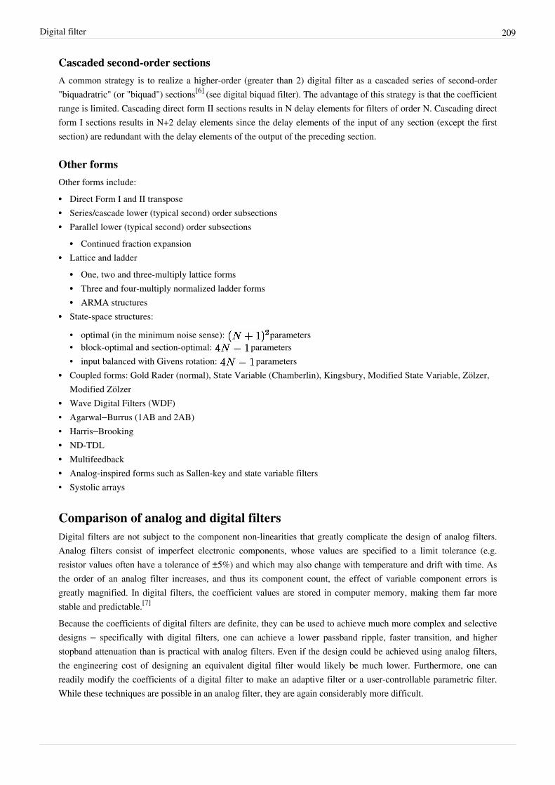
Digital filter 209
Cascaded second-order sectionsA common strategy is to realize a higher-order (greater than 2) digital filter as a cascaded series of second-order"biquadratric" (or "biquad") sections[6] (see digital biquad filter). The advantage of this strategy is that the coefficientrange is limited. Cascading direct form II sections results in N delay elements for filters of order N. Cascading directform I sections results in N+2 delay elements since the delay elements of the input of any section (except the firstsection) are redundant with the delay elements of the output of the preceding section.
Other formsOther forms include:•• Direct Form I and II transpose•• Series/cascade lower (typical second) order subsections•• Parallel lower (typical second) order subsections
•• Continued fraction expansion•• Lattice and ladder
•• One, two and three-multiply lattice forms•• Three and four-multiply normalized ladder forms•• ARMA structures
•• State-space structures:
• optimal (in the minimum noise sense): parameters• block-optimal and section-optimal: parameters• input balanced with Givens rotation: parameters
•• Coupled forms: Gold Rader (normal), State Variable (Chamberlin), Kingsbury, Modified State Variable, Zölzer,Modified Zölzer
•• Wave Digital Filters (WDF)• Agarwal–Burrus (1AB and 2AB)• Harris–Brooking•• ND-TDL•• Multifeedback•• Analog-inspired forms such as Sallen-key and state variable filters• Systolic arrays
Comparison of analog and digital filtersDigital filters are not subject to the component non-linearities that greatly complicate the design of analog filters.Analog filters consist of imperfect electronic components, whose values are specified to a limit tolerance (e.g.resistor values often have a tolerance of ±5%) and which may also change with temperature and drift with time. Asthe order of an analog filter increases, and thus its component count, the effect of variable component errors isgreatly magnified. In digital filters, the coefficient values are stored in computer memory, making them far morestable and predictable.[7]
Because the coefficients of digital filters are definite, they can be used to achieve much more complex and selectivedesigns – specifically with digital filters, one can achieve a lower passband ripple, faster transition, and higherstopband attenuation than is practical with analog filters. Even if the design could be achieved using analog filters,the engineering cost of designing an equivalent digital filter would likely be much lower. Furthermore, one canreadily modify the coefficients of a digital filter to make an adaptive filter or a user-controllable parametric filter.While these techniques are possible in an analog filter, they are again considerably more difficult.
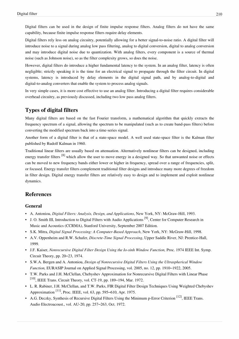
Digital filter 210
Digital filters can be used in the design of finite impulse response filters. Analog filters do not have the samecapability, because finite impulse response filters require delay elements.Digital filters rely less on analog circuitry, potentially allowing for a better signal-to-noise ratio. A digital filter willintroduce noise to a signal during analog low pass filtering, analog to digital conversion, digital to analog conversionand may introduce digital noise due to quantization. With analog filters, every component is a source of thermalnoise (such as Johnson noise), so as the filter complexity grows, so does the noise.However, digital filters do introduce a higher fundamental latency to the system. In an analog filter, latency is oftennegligible; strictly speaking it is the time for an electrical signal to propagate through the filter circuit. In digitalsystems, latency is introduced by delay elements in the digital signal path, and by analog-to-digital anddigital-to-analog converters that enable the system to process analog signals.In very simple cases, it is more cost effective to use an analog filter. Introducing a digital filter requires considerableoverhead circuitry, as previously discussed, including two low pass analog filters.
Types of digital filtersMany digital filters are based on the fast Fourier transform, a mathematical algorithm that quickly extracts thefrequency spectrum of a signal, allowing the spectrum to be manipulated (such as to create band-pass filters) beforeconverting the modified spectrum back into a time-series signal.Another form of a digital filter is that of a state-space model. A well used state-space filter is the Kalman filterpublished by Rudolf Kalman in 1960.Traditional linear filters are usually based on attenuation. Alternatively nonlinear filters can be designed, includingenergy transfer filters [8] which allow the user to move energy in a designed way. So that unwanted noise or effectscan be moved to new frequency bands either lower or higher in frequency, spread over a range of frequencies, split,or focused. Energy transfer filters complement traditional filter designs and introduce many more degrees of freedomin filter design. Digital energy transfer filters are relatively easy to design and to implement and exploit nonlineardynamics.
References
General• A. Antoniou, Digital Filters: Analysis, Design, and Applications, New York, NY: McGraw-Hill, 1993.• J. O. Smith III, Introduction to Digital Filters with Audio Applications [9], Center for Computer Research in
Music and Acoustics (CCRMA), Stanford University, September 2007 Edition.• S.K. Mitra, Digital Signal Processing: A Computer-Based Approach, New York, NY: McGraw-Hill, 1998.• A.V. Oppenheim and R.W. Schafer, Discrete-Time Signal Processing, Upper Saddle River, NJ: Prentice-Hall,
1999.• J.F. Kaiser, Nonrecursive Digital Filter Design Using the Io-sinh Window Function, Proc. 1974 IEEE Int. Symp.
Circuit Theory, pp. 20–23, 1974.• S.W.A. Bergen and A. Antoniou, Design of Nonrecursive Digital Filters Using the Ultraspherical Window
Function, EURASIP Journal on Applied Signal Processing, vol. 2005, no. 12, pp. 1910–1922, 2005.• T.W. Parks and J.H. McClellan, Chebyshev Approximation for Nonrecursive Digital Filters with Linear Phase
[10], IEEE Trans. Circuit Theory, vol. CT-19, pp. 189–194, Mar. 1972.• L. R. Rabiner, J.H. McClellan, and T.W. Parks, FIR Digital Filter Design Techniques Using Weighted Chebyshev
Approximation [11], Proc. IEEE, vol. 63, pp. 595–610, Apr. 1975.• A.G. Deczky, Synthesis of Recursive Digital Filters Using the Minimum p-Error Criterion [12], IEEE Trans.
Audio Electroacoust., vol. AU-20, pp. 257–263, Oct. 1972.
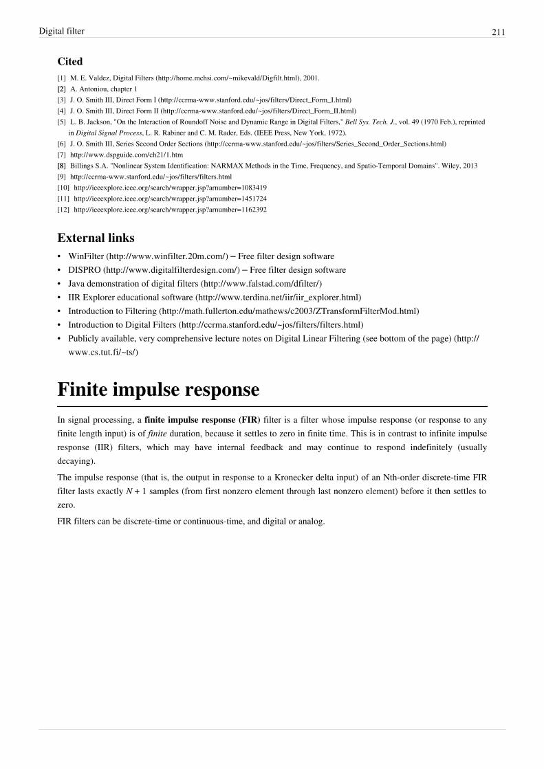
Digital filter 211
Cited[1] M. E. Valdez, Digital Filters (http:/ / home. mchsi. com/ ~mikevald/ Digfilt. html), 2001.[2][2] A. Antoniou, chapter 1[3] J. O. Smith III, Direct Form I (http:/ / ccrma-www. stanford. edu/ ~jos/ filters/ Direct_Form_I. html)[4] J. O. Smith III, Direct Form II (http:/ / ccrma-www. stanford. edu/ ~jos/ filters/ Direct_Form_II. html)[5] L. B. Jackson, "On the Interaction of Roundoff Noise and Dynamic Range in Digital Filters," Bell Sys. Tech. J., vol. 49 (1970 Feb.), reprinted
in Digital Signal Process, L. R. Rabiner and C. M. Rader, Eds. (IEEE Press, New York, 1972).[6] J. O. Smith III, Series Second Order Sections (http:/ / ccrma-www. stanford. edu/ ~jos/ filters/ Series_Second_Order_Sections. html)[7] http:/ / www. dspguide. com/ ch21/ 1. htm[8][8] Billings S.A. "Nonlinear System Identification: NARMAX Methods in the Time, Frequency, and Spatio-Temporal Domains". Wiley, 2013[9] http:/ / ccrma-www. stanford. edu/ ~jos/ filters/ filters. html[10] http:/ / ieeexplore. ieee. org/ search/ wrapper. jsp?arnumber=1083419[11] http:/ / ieeexplore. ieee. org/ search/ wrapper. jsp?arnumber=1451724[12] http:/ / ieeexplore. ieee. org/ search/ wrapper. jsp?arnumber=1162392
External links• WinFilter (http:/ / www. winfilter. 20m. com/ ) – Free filter design software• DISPRO (http:/ / www. digitalfilterdesign. com/ ) – Free filter design software• Java demonstration of digital filters (http:/ / www. falstad. com/ dfilter/ )• IIR Explorer educational software (http:/ / www. terdina. net/ iir/ iir_explorer. html)• Introduction to Filtering (http:/ / math. fullerton. edu/ mathews/ c2003/ ZTransformFilterMod. html)• Introduction to Digital Filters (http:/ / ccrma. stanford. edu/ ~jos/ filters/ filters. html)• Publicly available, very comprehensive lecture notes on Digital Linear Filtering (see bottom of the page) (http:/ /
www. cs. tut. fi/ ~ts/ )
Finite impulse responseIn signal processing, a finite impulse response (FIR) filter is a filter whose impulse response (or response to anyfinite length input) is of finite duration, because it settles to zero in finite time. This is in contrast to infinite impulseresponse (IIR) filters, which may have internal feedback and may continue to respond indefinitely (usuallydecaying).The impulse response (that is, the output in response to a Kronecker delta input) of an Nth-order discrete-time FIRfilter lasts exactly N + 1 samples (from first nonzero element through last nonzero element) before it then settles tozero.FIR filters can be discrete-time or continuous-time, and digital or analog.
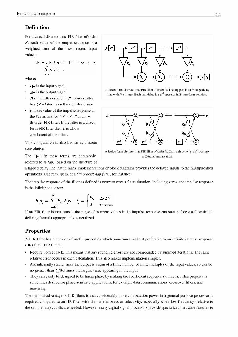
Finite impulse response 212
Definition
A direct form discrete-time FIR filter of order N. The top part is an N-stage delayline with N + 1 taps. Each unit delay is a z−1 operator in Z-transform notation.
A lattice form discrete-time FIR filter of order N. Each unit delay is a z−1 operatorin Z-transform notation.
For a causal discrete-time FIR filter of orderN, each value of the output sequence is aweighted sum of the most recent inputvalues:
where:
• is the input signal,• is the output signal,• is the filter order; an th-order filter
has terms on the right-hand side• is the value of the impulse response at
the i'th instant for of an th-order FIR filter. If the filter is a directform FIR filter then is also acoefficient of the filter .
This computation is also known as discreteconvolution.
The in these terms are commonlyreferred to as taps, based on the structure ofa tapped delay line that in many implementations or block diagrams provides the delayed inputs to the multiplicationoperations. One may speak of a 5th order/6-tap filter, for instance.
The impulse response of the filter as defined is nonzero over a finite duration. Including zeros, the impulse responseis the infinite sequence:
If an FIR filter is non-causal, the range of nonzero values in its impulse response can start before n = 0, with thedefining formula appropriately generalized.
PropertiesA FIR filter has a number of useful properties which sometimes make it preferable to an infinite impulse response(IIR) filter. FIR filters:•• Require no feedback. This means that any rounding errors are not compounded by summed iterations. The same
relative error occurs in each calculation. This also makes implementation simpler.• Are inherently stable, since the output is a sum of a finite number of finite multiples of the input values, so can be
no greater than times the largest value appearing in the input.• They can easily be designed to be linear phase by making the coefficient sequence symmetric. This property is
sometimes desired for phase-sensitive applications, for example data communications, crossover filters, andmastering.
The main disadvantage of FIR filters is that considerably more computation power in a general purpose processor is required compared to an IIR filter with similar sharpness or selectivity, especially when low frequency (relative to the sample rate) cutoffs are needed. However many digital signal processors provide specialized hardware features to

Finite impulse response 213
make FIR filters approximately as efficient as IIR for many applications.
Frequency responseThe filter's effect on the x[n] sequence is described in the frequency domain by the Convolution theorem:
and
where operators and respectively denote the discrete-time Fourier transform (DTFT) and its inverse.Therefore, complex-valued, multiplicative function is the filter's frequency response. It is defined by aFourier series:
where the added subscript denotes 2π-periodicity. Here represents frequency in normalized units(radians/sample). The substitution favored by many filter design programs, changes the units offrequency to cycles/sample and the periodicity to 1.[1] When the x[n] sequence has a known sampling-rate, samples/second, the substitution changes the units of frequency to cycles/second (hertz) andthe periodicity to The value corresponds to a frequency of Hz cycles/sample, which
is the Nyquist frequency.
Transfer functionThe frequency response can also be written as where function is the Z-transform ofthe impulse response:
z is a complex variable, and H(z) is a surface. One cycle of the periodic frequency response can be found in theregion defined by which is the unit circle of the z-plane. Filter transfer functions are oftenused to verify the stability of IIR designs. As we have already noted, FIR designs are inherently stable.
Filter designA FIR filter is designed by finding the coefficients and filter order that meet certain specifications, which can be inthe time-domain (e.g. a matched filter) and/or the frequency domain (most common). Matched filters perform across-correlation between the input signal and a known pulse-shape. The FIR convolution is a cross-correlationbetween the input signal and a time-reversed copy of the impulse-response. Therefore, the matched-filter's impulseresponse is "designed" by sampling the known pulse-shape and using those samples in reverse order as thecoefficients of the filter.[2]
When a particular frequency response is desired, several different design methods are common:1.1. Window design method2.2. Frequency Sampling method3.3. Weighted least squares design4. Parks-McClellan method (also known as the Equiripple, Optimal, or Minimax method). The Remez exchange
algorithm is commonly used to find an optimal equiripple set of coefficients. Here the user specifies a desired frequency response, a weighting function for errors from this response, and a filter order N. The algorithm then finds the set of coefficients that minimize the maximum deviation from the ideal. Intuitively, this finds the filter that is as close as you can get to the desired response given that you can use only coefficients.
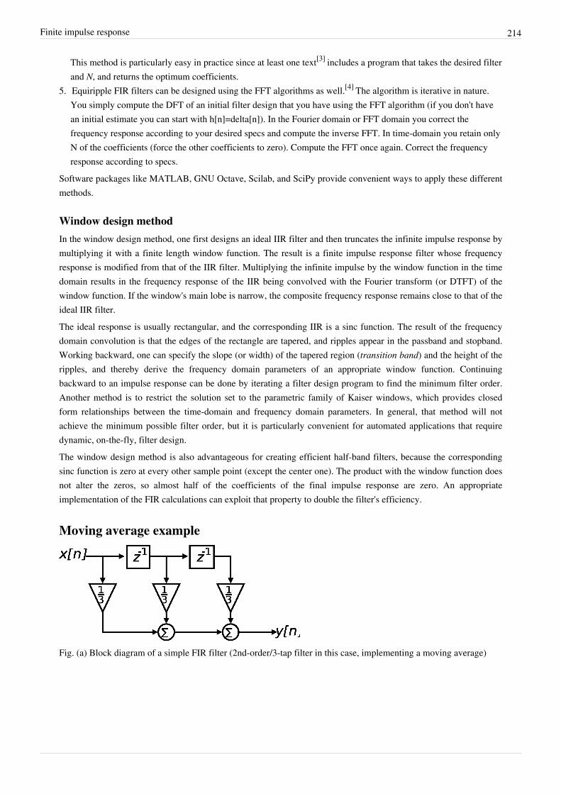
Finite impulse response 214
This method is particularly easy in practice since at least one text[3] includes a program that takes the desired filterand N, and returns the optimum coefficients.
5. Equiripple FIR filters can be designed using the FFT algorithms as well.[4] The algorithm is iterative in nature.You simply compute the DFT of an initial filter design that you have using the FFT algorithm (if you don't havean initial estimate you can start with h[n]=delta[n]). In the Fourier domain or FFT domain you correct thefrequency response according to your desired specs and compute the inverse FFT. In time-domain you retain onlyN of the coefficients (force the other coefficients to zero). Compute the FFT once again. Correct the frequencyresponse according to specs.
Software packages like MATLAB, GNU Octave, Scilab, and SciPy provide convenient ways to apply these differentmethods.
Window design methodIn the window design method, one first designs an ideal IIR filter and then truncates the infinite impulse response bymultiplying it with a finite length window function. The result is a finite impulse response filter whose frequencyresponse is modified from that of the IIR filter. Multiplying the infinite impulse by the window function in the timedomain results in the frequency response of the IIR being convolved with the Fourier transform (or DTFT) of thewindow function. If the window's main lobe is narrow, the composite frequency response remains close to that of theideal IIR filter.The ideal response is usually rectangular, and the corresponding IIR is a sinc function. The result of the frequencydomain convolution is that the edges of the rectangle are tapered, and ripples appear in the passband and stopband.Working backward, one can specify the slope (or width) of the tapered region (transition band) and the height of theripples, and thereby derive the frequency domain parameters of an appropriate window function. Continuingbackward to an impulse response can be done by iterating a filter design program to find the minimum filter order.Another method is to restrict the solution set to the parametric family of Kaiser windows, which provides closedform relationships between the time-domain and frequency domain parameters. In general, that method will notachieve the minimum possible filter order, but it is particularly convenient for automated applications that requiredynamic, on-the-fly, filter design.The window design method is also advantageous for creating efficient half-band filters, because the correspondingsinc function is zero at every other sample point (except the center one). The product with the window function doesnot alter the zeros, so almost half of the coefficients of the final impulse response are zero. An appropriateimplementation of the FIR calculations can exploit that property to double the filter's efficiency.
Moving average example
Fig. (a) Block diagram of a simple FIR filter (2nd-order/3-tap filter in this case, implementing a moving average)
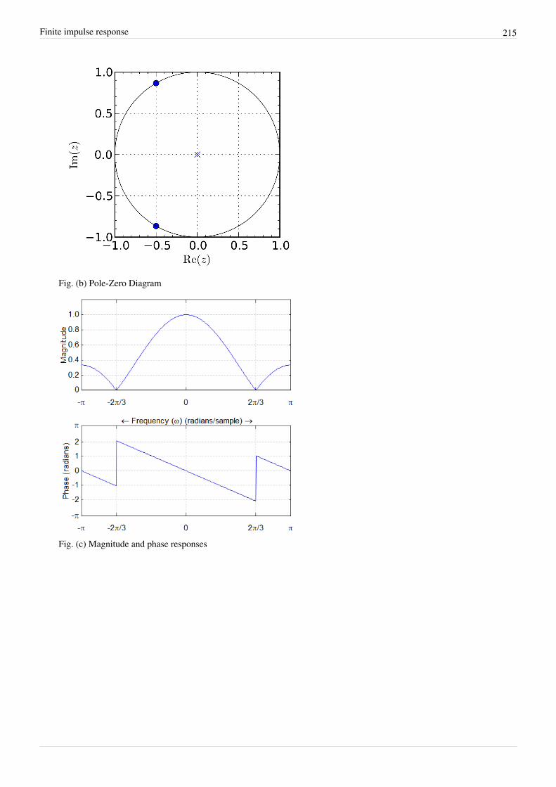
Finite impulse response 215
Fig. (b) Pole-Zero Diagram
Fig. (c) Magnitude and phase responses

Finite impulse response 216
Fig. (d) Amplitude and phase responsesA moving average filter is a very simple FIR filter. It is sometimes called a boxcar filter, especially when followedby decimation. The filter coefficients, , are found via the following equation:
To provide a more specific example, we select the filter order:
The impulse response of the resulting filter is:
The Fig. (a) on the right shows the block diagram of a 2nd-order moving-average filter discussed below. The transferfunction is:
Fig. (b) on the right shows the corresponding pole-zero diagram. Zero frequency (DC) corresponds to (1,0), positivefrequencies advancing counterclockwise around the circle to the Nyquist frequency at (-1,0). Two poles are locatedat the origin, and two zeros are located at , .The frequency response, in terms of normalized frequency ω, is:
Fig. (c) on the right shows the magnitude and phase components of But plots like these can also begenerated by doing a discrete Fourier transform (DFT) of the impulse response.[5] And because of symmetry, filterdesign or viewing software often displays only the [0,π] region. The magnitude plot indicates that themoving-average filter passes low frequencies with a gain near 1 and attenuates high frequencies, and is thus a crudelow-pass filter. The phase plot is linear except for discontinuities at the two frequencies where the magnitude goes tozero. The size of the discontinuities is π, indicating a sign reversal. They do not affect the property of linear phase.That fact is illustrated in Fig. (d).
Finite impulse response 217
Notes[1] A notable exception is Matlab, which prefers units of half-cycles/sample = cycles/2-samples, because the Nyquist frequency in those units is
1, a convenient choice for plotting software that displays the interval from 0 to the Nyquist frequency.[2][2] Oppenheim, Alan V., Willsky, Alan S., and Young, Ian T.,1983: Signals and Systems, p. 256 (Englewood Cliffs, New Jersey: Prentice-Hall,
Inc.) ISBN 0-13-809731-3[3][3] Rabiner, Lawrence R., and Gold, Bernard, 1975: Theory and Application of Digital Signal Processing (Englewood Cliffs, New Jersey:
Prentice-Hall, Inc.) ISBN 0-13-914101-4[4][4] A. E. Cetin, O.N. Gerek, Y. Yardimci, "Equiripple FIR filter design by the FFT algorithm," IEEE Signal Processing Magazine, pp. 60-64,
March 1997.[5] See Sampling the DTFT.
Citations
External links• Notes on the Optimal Design of FIR Filters (http:/ / cnx. org/ content/ col10553/ latest/ ) Connexions online book
by John Treichler (2008).• FIR FAQ (http:/ / dspguru. com/ dsp/ faqs/ fir) provided by dspguru.com.• BruteFIR; Software for applying long FIR filters to multi-channel digital audio, either offline or in realtime.
(http:/ / www. ludd. luth. se/ ~torger/ brutefir. html)• Freeverb3 Reverb Impulse Response Processor (http:/ / www. nongnu. org/ freeverb3/ )• Worked examples and explanation for designing FIR filters using windowing (http:/ / www. labbookpages. co.
uk/ audio/ firWindowing. html). Includes code examples.• A JAVA applet with different FIR-filters (http:/ / www. falstad. com/ dfilter/ ); the filters are applied to sound and
the results can be heard immediately. The source code is also available.• Matlab code (http:/ / signal. ee. bilkent. edu. tr/ my_filter. m); Matlab code for "Equiripple FIR filter design by
the FFT algorithm" by A. Enis Cetin, O. N. Gerek and Y. Yardimci, IEEE Signal Processing Magazine, 1997.

Infinite impulse response 218
Infinite impulse responseInfinite impulse response (IIR) is a property applying to many linear time-invariant systems. Common examples oflinear time-invariant systems are most electronic and digital filters. Systems with this property are known as IIRsystems or IIR filters, and are distinguished by having an impulse response which does not become exactly zero pasta certain point, but continues indefinitely. This is in contrast to a finite impulse response in which the impulseresponse h(t) does become exactly zero at times t > T for some finite T, thus being of finite duration.In practice, the impulse response even of IIR systems usually approaches zero and can be neglected past a certainpoint. However the physical systems which give rise to IIR or FIR (finite impulse response) responses are dissimilar,and therein lies the importance of the distinction. For instance, analog electronic filters composed of resistors,capacitors, and/or inductors (and perhaps linear amplifiers) are generally IIR filters. On the other hand, discrete-timefilters (usually digital filters) based on a tapped delay line employing no feedback are necessarily FIR filters. Thecapacitors (or inductors) in the analog filter have a "memory" and their internal state never completely relaxesfollowing an impulse. But in the latter case, after an impulse has reached the end of the tapped delay line, the systemhas no further memory of that impulse and has returned to its initial state; its impulse response beyond that point isexactly zero.
Implementation and designAlthough almost all analog electronic filters are IIR, digital filters may be either IIR or FIR. The presence offeedback in the topology of a discrete-time filter (such as the block diagram shown below) generally creates an IIRresponse. The z domain transfer function of an IIR filter contains a non-trivial denominator, describing thosefeedback terms. The transfer function of an FIR filter, on the other hand, has only a numerator as expressed in thegeneral form derived below. All of the coefficients (feedback terms) are zero and the filter has no finite poles.The transfer functions pertaining to IIR analog electronic filters have been extensively studied and optimized fortheir amplitude and phase characteristics. These continuous-time filter functions are described in the Laplacedomain. Desired solutions can be transferred to the case of discrete-time filters whose transfer functions areexpressed in the z domain, through the use of certain mathematical techniques such as the bilinear transform,impulse invariance, or pole–zero matching method. Thus digital IIR filters can be based on well-known solutions foranalog filters such as the Chebyshev filter, Butterworth filter, and Elliptic filter, inheriting the characteristics of thosesolutions.
Transfer function derivationDigital filters are often described and implemented in terms of the difference equation that defines how the outputsignal is related to the input signal:
where:• is the feedforward filter order• are the feedforward filter coefficients• is the feedback filter order• are the feedback filter coefficients• is the input signal• is the output signal.

Infinite impulse response 219
A more condensed form of the difference equation is:
which, when rearranged, becomes:
To find the transfer function of the filter, we first take the Z-transform of each side of the above equation, where weuse the time-shift property to obtain:
We define the transfer function to be:
Considering that in most IIR filter designs coefficient is 1, the IIR filter transfer function takes the moretraditional form:
Description of block diagram
Simple IIR filter block diagram
A typical block diagram of an IIR filter looks like thefollowing. The block is a unit delay. Thecoefficients and number of feedback/feedforward pathsare implementation-dependent.
Stability
The transfer function allows us to judge whether or nota system is bounded-input, bounded-output (BIBO)stable. To be specific, the BIBO stability criteriarequires that the ROC of the system includes the unitcircle. For example, for a causal system, all poles of thetransfer function have to have an absolute value smallerthan one. In other words, all poles must be locatedwithin a unit circle in the -plane.
The poles are defined as the values of which make the denominator of equal to 0:
Clearly, if then the poles are not located at the origin of the z-plane. This is in contrast to the FIR filterwhere all poles are located at the origin, and is therefore always stable.

Infinite impulse response 220
IIR filters are sometimes preferred over FIR filters because an IIR filter can achieve a much sharper transition regionroll-off than FIR filter of the same order.
ExampleLet the transfer function of a discrete-time filter be given by:
governed by the parameter , a real number with . is stable and causal with a pole at . Thetime-domain impulse response can be shown to be given by:
where is the unit step function. It can be seen that is non-zero for all , thus an impulse responsewhich continues infinitely.
Advantages and disadvantagesThe main advantage digital IIR filters have over FIR filters is their efficiency in implementation, in order to meet aspecification in terms of passband, stopband, ripple, and/or roll-off. Such a set of specifications can be accomplishedwith a lower order (Q in the above formulae) IIR filter than would be required for an FIR filter meeting the samerequirements. If implemented in a signal processor, this implies a correspondingly fewer number of calculations pertime step; the computational savings is often of a rather large factor.On the other hand, FIR filters can be easier to design, for instance, to match a particular frequency responserequirement. This is particularly true when the requirement is not one of the usual cases (high-pass, low-pass, notch,etc.) which have been studied and optimized for analog filters. Also FIR filters can be easily made to be linear phase(constant group delay vs frequency), a property that is not easily met using IIR filters and then only as anapproximation (for instance with the Bessel filter). Another issue regarding digital IIR filters is the potential for limitcycle behavior when idle, due to the feedback system in conjunction with quantization.
External links• The fifth module of the BORES Signal Processing DSP course - Introduction to DSP [1]
• IIR Digital Filter Design applet [2] in Java• IIR Digital Filter design tool [2] - produces coefficients, graphs, poles, zeros, and C code• Almafa.org Online IIR Design Tool [3] - does not require Java
References[1] http:/ / www. bores. com/ courses/ intro/ iir/ index. htm[2] http:/ / www-users. cs. york. ac. uk/ ~fisher/ mkfilter/[3] http:/ / almafa. org/ ?sidebar=docs/ iir. html

Nyquist ISI criterion 221
Nyquist ISI criterion
Raised cosine response meets the Nyquist ISI criterion. Consecutive raised-cosineimpulses demonstrate the zero ISI property between transmitted symbols at the samplinginstants. At t=0 the middle pulse is at its maximum and the sum of other impulses is zero.
In communications, the Nyquist ISIcriterion describes the conditionswhich, when satisfied by acommunication channel (includingresponses of transmit and receivefilters), result in no intersymbolinterference or ISI. It provides amethod for constructing band-limitedfunctions to overcome the effects ofintersymbol interference.
When consecutive symbols aretransmitted over a channel by a linearmodulation (such as ASK, QAM, etc.), the impulse response (or equivalently the frequency response) of the channelcauses a transmitted symbol to be spread in the time domain. This causes intersymbol interference because thepreviously transmitted symbols affect the currently received symbol, thus reducing tolerance for noise. The Nyquisttheorem relates this time-domain condition to an equivalent frequency-domain condition.
The Nyquist criterion is closely related to the Nyquist-Shannon sampling theorem, with only a differing point ofview.
Nyquist criterionIf we denote the channel impulse response as , then the condition for an ISI-free response can be expressed as:
for all integers , where is the symbol period. The Nyquist theorem says that this is equivalent to:
,
where is the Fourier transform of . This is the Nyquist ISI criterion.This criterion can be intuitively understood in the following way: frequency-shifted replicas of H(f) must add up to aconstant value.In practice this criterion is applied to baseband filtering by regarding the symbol sequence as weighted impulses(Dirac delta function). When the baseband filters in the communication system satisfy the Nyquist criterion, symbolscan be transmitted over a channel with flat response within a limited frequency band, without ISI. Examples of suchbaseband filters are the raised-cosine filter, or the sinc filter as the ideal case.

Nyquist ISI criterion 222
DerivationTo derive the criterion, we first express the received signal in terms of the transmitted symbol and the channelresponse. Let the function h(t) be the channel impulse response, x[n] the symbols to be sent, with a symbol period ofTs; the received signal y(t) will be in the form (where noise has been ignored for simplicity):
.
Sampling this signal at intervals of Ts, we can express y(t) as a discrete-time equation:
.
If we write the h[0] term of the sum separately, we can express this as:
,
and from this we can conclude that if a response h[n] satisfies
,
only one transmitted symbol has an effect on the received y[k] at sampling instants, thus removing any ISI. This isthe time-domain condition for an ISI-free channel. Now we find a frequency-domain equivalent for it. We start byexpressing this condition in continuous time:
for all integer . We multiply such a h(t) by a sum of Dirac delta function (impulses) separated by intervals TsThis is equivalent of sampling the response as above but using a continuous time expression. The right side of thecondition can then be expressed as one impulse in the origin:
Fourier transforming both members of this relationship we obtain:
and
.
This is the Nyquist ISI criterion and, if a channel response satisfies it, then there is no ISI between the differentsamples.
References• John G. Proakis, "Digital Communications, 3rd Edition", McGraw-Hill Book Co., 1995. ISBN 0-07-113814-5• Behzad Razavi, "RF Microelectronics", Prentice-Hall, Inc., 1998. ISBN 0-13-887571-5
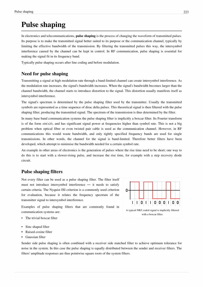
Pulse shaping 223
Pulse shapingIn electronics and telecommunications, pulse shaping is the process of changing the waveform of transmitted pulses.Its purpose is to make the transmitted signal better suited to its purpose or the communication channel, typically bylimiting the effective bandwidth of the transmission. By filtering the transmitted pulses this way, the intersymbolinterference caused by the channel can be kept in control. In RF communication, pulse shaping is essential formaking the signal fit in its frequency band.Typically pulse shaping occurs after line coding and before modulation.
Need for pulse shapingTransmitting a signal at high modulation rate through a band-limited channel can create intersymbol interference. Asthe modulation rate increases, the signal's bandwidth increases. When the signal's bandwidth becomes larger than thechannel bandwidth, the channel starts to introduce distortion to the signal. This distortion usually manifests itself asintersymbol interference.The signal's spectrum is determined by the pulse shaping filter used by the transmitter. Usually the transmittedsymbols are represented as a time sequence of dirac delta pulses. This theoretical signal is then filtered with the pulseshaping filter, producing the transmitted signal. The spectrum of the transmission is thus determined by the filter.In many base band communication systems the pulse shaping filter is implicitly a boxcar filter. Its Fourier transformis of the form sin(x)/x, and has significant signal power at frequencies higher than symbol rate. This is not a bigproblem when optical fibre or even twisted pair cable is used as the communication channel. However, in RFcommunications this would waste bandwidth, and only tightly specified frequency bands are used for singletransmissions. In other words, the channel for the signal is band-limited. Therefore better filters have beendeveloped, which attempt to minimise the bandwidth needed for a certain symbol rate.An example in other areas of electronics is the generation of pulses where the rise time need to be short; one way todo this is to start with a slower-rising pulse, and increase the rise time, for example with a step recovery diodecircuit.
Pulse shaping filters
A typical NRZ coded signal is implicitly filteredwith a boxcar filter.
Not every filter can be used as a pulse shaping filter. The filter itselfmust not introduce intersymbol interference — it needs to satisfycertain criteria. The Nyquist ISI criterion is a commonly used criterionfor evaluation, because it relates the frequency spectrum of thetransmitter signal to intersymbol interference.
Examples of pulse shaping filters that are commonly found incommunication systems are:• The trivial boxcar filter
• Sinc shaped filter•• Raised-cosine filter•• Gaussian filterSender side pulse shaping is often combined with a receiver side matched filter to achieve optimum tolerance fornoise in the system. In this case the pulse shaping is equally distributed between the sender and receiver filters. Thefilters' amplitude responses are thus pointwise square roots of the system filters.

Pulse shaping 224
Other approaches that eliminate complex pulse shaping filters have been invented. In OFDM, the carriers aremodulated so slowly that each carrier is virtually unaffected by the bandwidth limitation of the channel.
Boxcar filterThe boxcar filter results in infinitely wide bandwidth for the signal. Thus its usefulness is limited, but it is usedwidely in wired baseband communications, where the channel has some extra bandwidth and the distortion createdby the channel can be tolerated.
Sinc filterMain article: sinc filter
Amplitude response of raised-cosine filter with various roll-off factors
Theoretically the best pulse shapingfilter would be the sinc filter, but itcannot be implemented precisely. It isa non-causal filter with relativelyslowly decaying tails. It is alsoproblematic from a synchronisationpoint of view as any phase error resultsin steeply increasing intersymbolinterference.
Raised-cosine filter
Main article: raised-cosine filterRaised-cosine filters are practical to implement and they are in wide use. They have a configurable excessbandwidth, so communication systems can choose a trade off between a simpler filter and spectral efficiency.
Gaussian filterMain article: Gaussian filterThis gives an output pulse shaped like a Gaussian function.
References• John G. Proakis, "Digital Communications, 3rd Edition" Chapter 9, McGraw-Hill Book Co., 1995. ISBN
0-07-113814-5• National Instruments Signal Generator Tutorial, Pulse Shaping to Improve Spectral Efficiency [1]
• National Instruments Measurement Fundamentals Tutorial, Pulse-Shape Filtering in Communications Systems [2]
References[1] http:/ / zone. ni. com/ devzone/ cda/ ph/ p/ id/ 200[2] http:/ / zone. ni. com/ devzone/ cda/ tut/ p/ id/ 3876
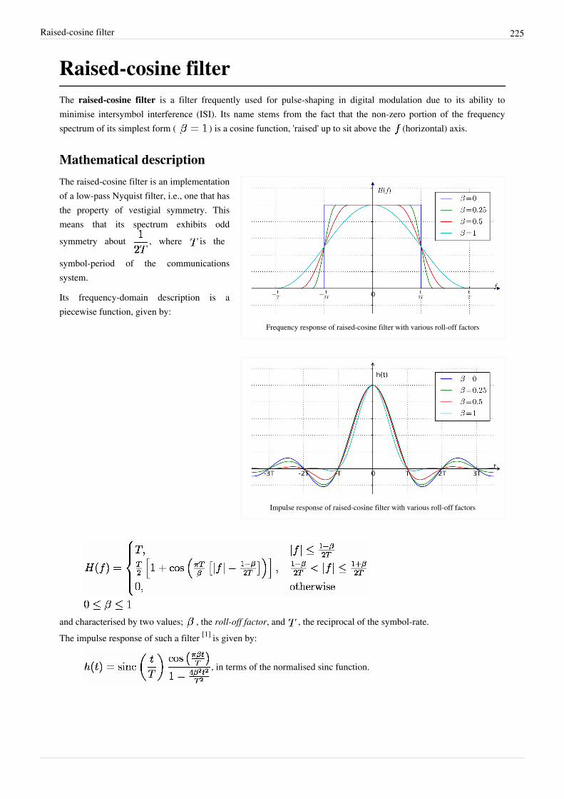
Raised-cosine filter 225
Raised-cosine filterThe raised-cosine filter is a filter frequently used for pulse-shaping in digital modulation due to its ability tominimise intersymbol interference (ISI). Its name stems from the fact that the non-zero portion of the frequencyspectrum of its simplest form ( ) is a cosine function, 'raised' up to sit above the (horizontal) axis.
Mathematical description
Frequency response of raised-cosine filter with various roll-off factors
Impulse response of raised-cosine filter with various roll-off factors
The raised-cosine filter is an implementationof a low-pass Nyquist filter, i.e., one that hasthe property of vestigial symmetry. Thismeans that its spectrum exhibits oddsymmetry about , where is the
symbol-period of the communicationssystem.
Its frequency-domain description is apiecewise function, given by:
and characterised by two values; , the roll-off factor, and , the reciprocal of the symbol-rate.The impulse response of such a filter [1] is given by:
, in terms of the normalised sinc function.

Raised-cosine filter 226
Roll-off factor
The roll-off factor, , is a measure of the excess bandwidth of the filter, i.e. the bandwidth occupied beyond the
Nyquist bandwidth of . If we denote the excess bandwidth as , then:
where is the symbol-rate.
The graph shows the amplitude response as is varied between 0 and 1, and the corresponding effect on theimpulse response. As can be seen, the time-domain ripple level increases as decreases. This shows that the excessbandwidth of the filter can be reduced, but only at the expense of an elongated impulse response.
As approaches 0, the roll-off zone becomes infinitesimally narrow, hence:
where is the rectangular function, so the impulse response approaches . Hence, it converges to
an ideal or brick-wall filter in this case.
When , the non-zero portion of the spectrum is a pure raised cosine, leading to the simplification:
BandwidthThe bandwidth of a raised cosine filter is most commonly defined as the width of the non-zero portion of itsspectrum, i.e.:
(0<T<1)
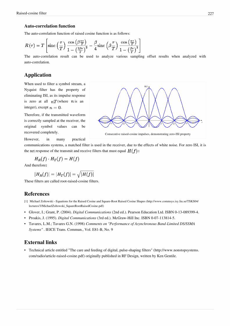
Raised-cosine filter 227
Auto-correlation functionThe auto-correlation function of raised cosine function is as follows:
The auto-correlation result can be used to analyze various sampling offset results when analyzed withauto-correlation.
Application
Consecutive raised-cosine impulses, demonstrating zero-ISI property
When used to filter a symbol stream, aNyquist filter has the property ofeliminating ISI, as its impulse responseis zero at all (where is aninteger), except .
Therefore, if the transmitted waveformis correctly sampled at the receiver, theoriginal symbol values can berecovered completely.However, in many practicalcommunications systems, a matched filter is used in the receiver, due to the effects of white noise. For zero ISI, it isthe net response of the transmit and receive filters that must equal :
And therefore:
These filters are called root-raised-cosine filters.
References[1] Michael Zoltowski - Equations for the Raised Cosine and Square-Root Raised Cosine Shapes (http:/ / www. commsys. isy. liu. se/ TSKS04/
lectures/ 3/ MichaelZoltowski_SquareRootRaisedCosine. pdf)
• Glover, I.; Grant, P. (2004). Digital Communications (2nd ed.). Pearson Education Ltd. ISBN 0-13-089399-4.• Proakis, J. (1995). Digital Communications (3rd ed.). McGraw-Hill Inc. ISBN 0-07-113814-5.• Tavares, L.M.; Tavares G.N. (1998) Comments on "Performance of Asynchronous Band-Limited DS/SSMA
Systems" . IEICE Trans. Commun., Vol. E81-B, No. 9
External links• Technical article entitled "The care and feeding of digital, pulse-shaping filters" (http:/ / www. nonstopsystems.
com/ radio/ article-raised-cosine. pdf) originally published in RF Design, written by Ken Gentile.
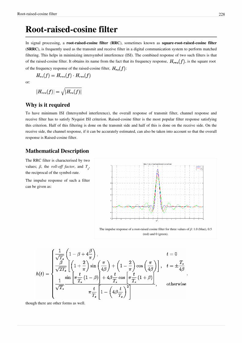
Root-raised-cosine filter 228
Root-raised-cosine filterIn signal processing, a root-raised-cosine filter (RRC), sometimes known as square-root-raised-cosine filter(SRRC), is frequently used as the transmit and receive filter in a digital communication system to perform matchedfiltering. This helps in minimizing intersymbol interference (ISI). The combined response of two such filters is thatof the raised-cosine filter. It obtains its name from the fact that its frequency response, , is the square rootof the frequency response of the raised-cosine filter, :
or:
Why is it requiredTo have minimum ISI (Intersymbol interference), the overall response of transmit filter, channel response andreceive filter has to satisfy Nyquist ISI criterion. Raised-cosine filter is the most popular filter response satisfyingthis criterion. Half of this filtering is done on the transmit side and half of this is done on the receive side. On thereceive side, the channel response, if it can be accurately estimated, can also be taken into account so that the overallresponse is Raised-cosine filter.
Mathematical Description
The impulse response of a root-raised cosine filter for three values of β: 1.0 (blue), 0.5(red) and 0 (green).
The RRC filter is characterised by twovalues; β, the roll-off factor, and Ts,the reciprocal of the symbol-rate.
The impulse response of such a filtercan be given as:
,
though there are other forms as well.

Root-raised-cosine filter 229
Unlike the raised-cosine filter, the impulse response is not zero at the intervals of ±Ts. However, the combinedtransmit and receive filters form a raised-cosine filter which does have zero at the intervals of ±Ts. Only in the caseof β=0 does the root raised-cosine have zeros at ±Ts.
References•• S. Daumont, R. Basel, Y. Lout, "Root-Raised Cosine filter influences on PAPR distribution of single carrier
signals", ISCCSP 2008, Malta, 12-14 March 2008.• Proakis, J. (1995). Digital Communications (3rd ed.). McGraw-Hill Inc. ISBN 0-07-113814-5.
Adaptive filterAn adaptive filter is a system with a linear filter that has a transfer function controlled by variable parameters and ameans to adjust those parameters according to an optimization algorithm. Because of the complexity of theoptimization algorithms, most adaptive filters are digital filters. Adaptive filters are required for some applicationsbecause some parameters of the desired processing operation (for instance, the locations of reflective surfaces in areverberant space) are not known in advance or are changing. The closed loop adaptive filter uses feedback in theform of an error signal to refine its transfer function.Generally speaking, the closed loop adaptive process involves the use of a cost function, which is a criterion foroptimum performance of the filter, to feed an algorithm, which determines how to modify filter transfer function tominimize the cost on the next iteration. The most common cost function is the mean square of the error signal.As the power of digital signal processors has increased, adaptive filters have become much more common and arenow routinely used in devices such as mobile phones and other communication devices, camcorders and digitalcameras, and medical monitoring equipment.
Example applicationThe recording of a heart beat (an ECG), may be corrupted by noise from the AC mains. The exact frequency of thepower and its harmonics may vary from moment to moment.One way to remove the noise is to filter the signal with a notch filter at the mains frequency and its vicinity, whichcould excessively degrade the quality of the ECG since the heart beat would also likely have frequency componentsin the rejected range.To circumvent this potential loss of information, an adaptive filter could be used. The adaptive filter would takeinput both from the patient and from the mains and would thus be able to track the actual frequency of the noise as itfluctuates and subtract the noise from the recording. Such an adaptive technique generally allows for a filter with asmaller rejection range, which means, in this case, that the quality of the output signal is more accurate for medicalpurposes.
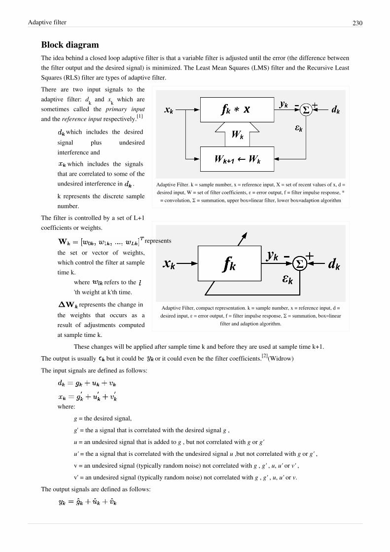
Adaptive filter 230
Block diagramThe idea behind a closed loop adaptive filter is that a variable filter is adjusted until the error (the difference betweenthe filter output and the desired signal) is minimized. The Least Mean Squares (LMS) filter and the Recursive LeastSquares (RLS) filter are types of adaptive filter.
Adaptive Filter. k = sample number, x = reference input, X = set of recent values of x, d =desired input, W = set of filter coefficients, ε = error output, f = filter impulse response, *
= convolution, Σ = summation, upper box=linear filter, lower box=adaption algorithm
Adaptive Filter, compact representation. k = sample number, x = reference input, d =desired input, ε = error output, f = filter impulse response, Σ = summation, box=linear
filter and adaption algorithm.
There are two input signals to theadaptive filter: dk and xk which aresometimes called the primary inputand the reference input respectively.[1]
which includes the desiredsignal plus undesiredinterference and
which includes the signalsthat are correlated to some of theundesired interference in .
k represents the discrete samplenumber.
The filter is controlled by a set of L+1coefficients or weights.
representsthe set or vector of weights,which control the filter at sampletime k.
where refers to the 'th weight at k'th time.
represents the change inthe weights that occurs as aresult of adjustments computedat sample time k.
These changes will be applied after sample time k and before they are used at sample time k+1.The output is usually but it could be or it could even be the filter coefficients.[2](Widrow)The input signals are defined as follows:
where:g = the desired signal,g' = the a signal that is correlated with the desired signal g ,u = an undesired signal that is added to g , but not correlated with g or g'
u' = the a signal that is correlated with the undesired signal u ,but not correlated with g or g' ,v = an undesired signal (typically random noise) not correlated with g , g' , u, u' or v' ,v' = an undesired signal (typically random noise) not correlated with g , g' , u, u' or v.
The output signals are defined as follows:

Adaptive filter 231
.where:
= the output of the filter if the input was only g' ,= the output of the filter if the input was only u' ,= the output of the filter if the input was only v' .
Tapped delay line FIR filterIf the variable filter has a tapped delay line Finite Impulse Response (FIR) structure, then the impulse response isequal to the filter coefficients. The output of the filter is given by
where refers to the 'th weight at k'th time.
Ideal case
In the ideal case . All the undesired signals in are represented by . consistsentirely of a signal correlated with the undesired signal in .The output of the variable filter in the ideal case is
.The error signal or cost function is the difference between and
. The desired signal gk passes through without being changed.
The error signal is minimized in the mean square sense when is minimized. In other words, is thebest mean square estimate of . In the ideal case, and . In the ideal case, all that is left afterthe subtraction is which is the unchanged desired signal with all undesired signals removed.
Signal components in the reference inputIn some situations, the reference input x_k includes components of the desired signal. This means g' ≠ 0.Perfect cancelation of the undesired interference is not possible in the case, but improvement of the signal tointerference ratio is possible. The output will be
. The desired signal will be modified (usually decreased).The output signal to interference ratio has a simple formula referred to as power inversion.
.
where
= output signal to interference ratio.= reference signal to interference ratio.
= frequency in the z-domain.This formula means that the output signal to interference ratio at a particular frequency is the reciprocal of thereference signal to interference ratio.[3]
Example: A fast food restaurant has a drive-up window. Before getting to the window, customers place their order by speaking into a microphone. The microphone also picks up noise from the engine and the environment. This microphone provides the primary signal. The signal power from the customer’s voice and the noise power from the engine are equal. It is difficult for the employees in the restaurant to understand the customer. To reduce the amount

Adaptive filter 232
of interference in the primary microphone, a second microphone is located where it is intended to pick up soundsfrom the engine. It also picks up the customer’s voice. This microphone is the source of the reference signal. In thiscase, the engine noise is 50 times more powerful than the customer’s voice. Once the canceler has converged, theprimary signal to interference ratio will be improved from 1:1 to 50:1.
Adaptive Linear Combiner
Adaptive linear combiner showing the combiner and the adaption process. k = samplenumber, n=input variable index, x = reference inputs, d = desired input, W = set of filter
coefficients, ε = error output, Σ = summation, upper box=linear combiner, lowerbox=adaption algorithm.
Adaptive linear combiner, compact representation. k = sample number, n=input variableindex, x = reference inputs, d = desired input, ε = error output, Σ = summation.
The adaptive linear combiner (ALC)resembles the adaptive tapped delayline FIR filter except that there is noassumed relationship between the Xvalues. If the X values were from theoutputs of a tapped delay line, then thecombination of tapped delay line andALC would comprise an adaptivefilter. However, the X values could bethe values of an array of pixels. Orthey could be the outputs of multipletapped delay lines. The ALC finds useas an adaptive beam former for arraysof hydrophones or antennas.
where refers to the 'th weight at k'th time.
LMS algorithm
Main article: Least mean squares filterIf the variable filter has a tapped delayline FIR structure, then the LMSupdate algorithm is especially simple.Typically, after each sample, the coefficients of the FIR filter are adjusted as follows:[4](Widrow)
for
μ is called the convergence factor.The LMS algorithm does not require that the X values have any particular relationship; therefor it can be used toadapt a linear combiner as well as an FIR filter. In this case the update formula is written as:
The effect of the LMS algorithm is at each time, k, to make a small change in each weight. The direction of thechange is such that it would decrease the error if it had been applied at time k. The magnitude of the change in eachweight depends on μ, the associated X value and the error at time k. The weights making the largest contribution tothe output, , are changed the most. If the error is zero, then there should be no change in the weights. If theassociated value of X is zero, then changing the weight makes no difference, so it is not changed.
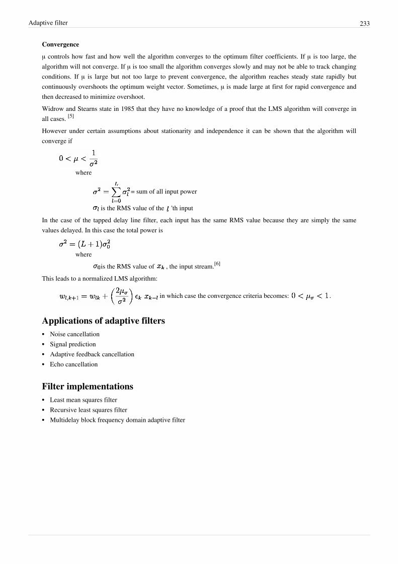
Adaptive filter 233
Convergence
μ controls how fast and how well the algorithm converges to the optimum filter coefficients. If μ is too large, thealgorithm will not converge. If μ is too small the algorithm converges slowly and may not be able to track changingconditions. If μ is large but not too large to prevent convergence, the algorithm reaches steady state rapidly butcontinuously overshoots the optimum weight vector. Sometimes, μ is made large at first for rapid convergence andthen decreased to minimize overshoot.Widrow and Stearns state in 1985 that they have no knowledge of a proof that the LMS algorithm will converge inall cases. [5]
However under certain assumptions about stationarity and independence it can be shown that the algorithm willconverge if
where
= sum of all input power
is the RMS value of the 'th inputIn the case of the tapped delay line filter, each input has the same RMS value because they are simply the samevalues delayed. In this case the total power is
whereis the RMS value of , the input stream.[6]
This leads to a normalized LMS algorithm:
in which case the convergence criteria becomes: .
Applications of adaptive filters•• Noise cancellation•• Signal prediction•• Adaptive feedback cancellation•• Echo cancellation
Filter implementations•• Least mean squares filter•• Recursive least squares filter•• Multidelay block frequency domain adaptive filter
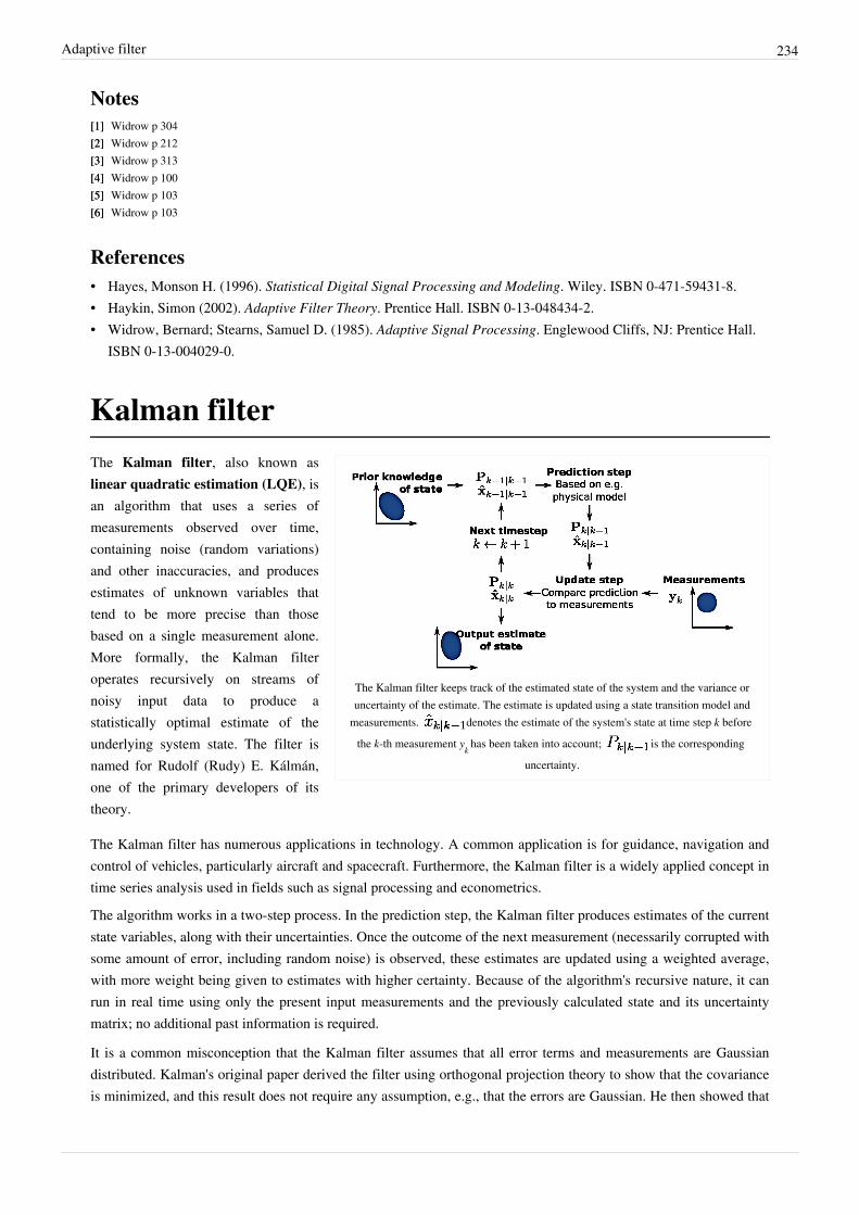
Adaptive filter 234
Notes[1][1] Widrow p 304[2][2] Widrow p 212[3][3] Widrow p 313[4][4] Widrow p 100[5][5] Widrow p 103[6][6] Widrow p 103
References• Hayes, Monson H. (1996). Statistical Digital Signal Processing and Modeling. Wiley. ISBN 0-471-59431-8.• Haykin, Simon (2002). Adaptive Filter Theory. Prentice Hall. ISBN 0-13-048434-2.• Widrow, Bernard; Stearns, Samuel D. (1985). Adaptive Signal Processing. Englewood Cliffs, NJ: Prentice Hall.
ISBN 0-13-004029-0.
Kalman filter
The Kalman filter keeps track of the estimated state of the system and the variance oruncertainty of the estimate. The estimate is updated using a state transition model and
measurements. denotes the estimate of the system's state at time step k before
the k-th measurement yk has been taken into account; is the corresponding
uncertainty.
The Kalman filter, also known aslinear quadratic estimation (LQE), isan algorithm that uses a series ofmeasurements observed over time,containing noise (random variations)and other inaccuracies, and producesestimates of unknown variables thattend to be more precise than thosebased on a single measurement alone.More formally, the Kalman filteroperates recursively on streams ofnoisy input data to produce astatistically optimal estimate of theunderlying system state. The filter isnamed for Rudolf (Rudy) E. Kálmán,one of the primary developers of itstheory.
The Kalman filter has numerous applications in technology. A common application is for guidance, navigation andcontrol of vehicles, particularly aircraft and spacecraft. Furthermore, the Kalman filter is a widely applied concept intime series analysis used in fields such as signal processing and econometrics.
The algorithm works in a two-step process. In the prediction step, the Kalman filter produces estimates of the currentstate variables, along with their uncertainties. Once the outcome of the next measurement (necessarily corrupted withsome amount of error, including random noise) is observed, these estimates are updated using a weighted average,with more weight being given to estimates with higher certainty. Because of the algorithm's recursive nature, it canrun in real time using only the present input measurements and the previously calculated state and its uncertaintymatrix; no additional past information is required.
It is a common misconception that the Kalman filter assumes that all error terms and measurements are Gaussiandistributed. Kalman's original paper derived the filter using orthogonal projection theory to show that the covarianceis minimized, and this result does not require any assumption, e.g., that the errors are Gaussian. He then showed that

Kalman filter 235
the filter yields the exact conditional probability estimate in the special case that all errors are Gaussian-distributed.Extensions and generalizations to the method have also been developed, such as the extended Kalman filter and theunscented Kalman filter which work on nonlinear systems. The underlying model is a Bayesian model similar to ahidden Markov model but where the state space of the latent variables is continuous and where all latent andobserved variables have Gaussian distributions.
Naming and historical developmentThe filter is named after Hungarian émigré Rudolf E. Kálmán, although Thorvald Nicolai Thiele[1][2] and PeterSwerling developed a similar algorithm earlier. Richard S. Bucy of the University of Southern California contributedto the theory, leading to it often being called the Kalman–Bucy filter. Stanley F. Schmidt is generally credited withdeveloping the first implementation of a Kalman filter. It was during a visit by Kalman to the NASA Ames ResearchCenter that he saw the applicability of his ideas to the problem of trajectory estimation for the Apollo program,leading to its incorporation in the Apollo navigation computer. This Kalman filter was first described and partiallydeveloped in technical papers by Swerling (1958), Kalman (1960) and Kalman and Bucy (1961).Kalman filters have been vital in the implementation of the navigation systems of U.S. Navy nuclear ballistic missilesubmarines, and in the guidance and navigation systems of cruise missiles such as the U.S. Navy's Tomahawkmissile and the U.S. Air Force's Air Launched Cruise Missile. It is also used in the guidance and navigation systemsof the NASA Space Shuttle and the attitude control and navigation systems of the International Space Station.This digital filter is sometimes called the Stratonovich–Kalman–Bucy filter because it is a special case of a moregeneral, non-linear filter developed somewhat earlier by the Soviet mathematician Ruslan L. Stratonovich.[3][4][5][6]
In fact, some of the special case linear filter's equations appeared in these papers by Stratonovich that were publishedbefore summer 1960, when Kalman met with Stratonovich during a conference in Moscow.
Overview of the calculationThe Kalman filter uses a system's dynamics model (e.g., physical laws of motion), known control inputs to thatsystem, and multiple sequential measurements (such as from sensors) to form an estimate of the system's varyingquantities (its state) that is better than the estimate obtained by using any one measurement alone. As such, it is acommon sensor fusion and data fusion algorithm.All measurements and calculations based on models are estimates to some degree. Noisy sensor data, approximationsin the equations that describe how a system changes, and external factors that are not accounted for introduce someuncertainty about the inferred values for a system's state. The Kalman filter averages a prediction of a system's statewith a new measurement using a weighted average. The purpose of the weights is that values with better (i.e.,smaller) estimated uncertainty are "trusted" more. The weights are calculated from the covariance, a measure of theestimated uncertainty of the prediction of the system's state. The result of the weighted average is a new stateestimate that lies between the predicted and measured state, and has a better estimated uncertainty than either alone.This process is repeated every time step, with the new estimate and its covariance informing the prediction used inthe following iteration. This means that the Kalman filter works recursively and requires only the last "best guess",rather than the entire history, of a system's state to calculate a new state.Because the certainty of the measurements is often difficult to measure precisely, it is common to discuss the filter'sbehavior in terms of gain. The Kalman gain is a function of the relative certainty of the measurements and currentstate estimate, and can be "tuned" to achieve particular performance. With a high gain, the filter places more weighton the measurements, and thus follows them more closely. With a low gain, the filter follows the model predictionsmore closely, smoothing out noise but decreasing the responsiveness. At the extremes, a gain of one causes the filterto ignore the state estimate entirely, while a gain of zero causes the measurements to be ignored.
Kalman filter 236
When performing the actual calculations for the filter (as discussed below), the state estimate and covariances arecoded into matrices to handle the multiple dimensions involved in a single set of calculations. This allows forrepresentation of linear relationships between different state variables (such as position, velocity, and acceleration) inany of the transition models or covariances.
Example applicationAs an example application, consider the problem of determining the precise location of a truck. The truck can beequipped with a GPS unit that provides an estimate of the position within a few meters. The GPS estimate is likely tobe noisy; readings 'jump around' rapidly, though always remaining within a few meters of the real position. Inaddition, since the truck is expected to follow the laws of physics, its position can also be estimated by integrating itsvelocity over time, determined by keeping track of wheel revolutions and the angle of the steering wheel. This is atechnique known as dead reckoning. Typically, dead reckoning will provide a very smooth estimate of the truck'sposition, but it will drift over time as small errors accumulate.In this example, the Kalman filter can be thought of as operating in two distinct phases: predict and update. In theprediction phase, the truck's old position will be modified according to the physical laws of motion (the dynamic or"state transition" model) plus any changes produced by the accelerator pedal and steering wheel. Not only will a newposition estimate be calculated, but a new covariance will be calculated as well. Perhaps the covariance isproportional to the speed of the truck because we are more uncertain about the accuracy of the dead reckoningestimate at high speeds but very certain about the position when moving slowly. Next, in the update phase, ameasurement of the truck's position is taken from the GPS unit. Along with this measurement comes some amount ofuncertainty, and its covariance relative to that of the prediction from the previous phase determines how much thenew measurement will affect the updated prediction. Ideally, if the dead reckoning estimates tend to drift away fromthe real position, the GPS measurement should pull the position estimate back towards the real position but notdisturb it to the point of becoming rapidly changing and noisy.
Technical description and contextThe Kalman filter is an efficient recursive filter that estimates the internal state of a linear dynamic system from aseries of noisy measurements. It is used in a wide range of engineering and econometric applications from radar andcomputer vision to estimation of structural macroeconomic models, and is an important topic in control theory andcontrol systems engineering. Together with the linear-quadratic regulator (LQR), the Kalman filter solves thelinear-quadratic-Gaussian control problem (LQG). The Kalman filter, the linear-quadratic regulator and thelinear-quadratic-Gaussian controller are solutions to what arguably are the most fundamental problems in controltheory.In most applications, the internal state is much larger (more degrees of freedom) than the few "observable"parameters which are measured. However, by combining a series of measurements, the Kalman filter can estimatethe entire internal state.In Dempster–Shafer theory, each state equation or observation is considered a special case of a linear belief functionand the Kalman filter is a special case of combining linear belief functions on a join-tree or Markov tree. Additionalapproaches include Belief Filters which use Bayes or evidential updates to the state equations.A wide variety of Kalman filters have now been developed, from Kalman's original formulation, now called the"simple" Kalman filter, the Kalman–Bucy filter, Schmidt's "extended" filter, the information filter, and a variety of"square-root" filters that were developed by Bierman, Thornton and many others. Perhaps the most commonly usedtype of very simple Kalman filter is the phase-locked loop, which is now ubiquitous in radios, especially frequencymodulation (FM) radios, television sets, satellite communications receivers, outer space communications systems,and nearly any other electronic communications equipment.

Kalman filter 237
Underlying dynamic system modelThe Kalman filters are based on linear dynamic systems discretized in the time domain. They are modelled on aMarkov chain built on linear operators perturbed by errors that may include Gaussian noise. The state of the systemis represented as a vector of real numbers. At each discrete time increment, a linear operator is applied to the state togenerate the new state, with some noise mixed in, and optionally some information from the controls on the system ifthey are known. Then, another linear operator mixed with more noise generates the observed outputs from the true("hidden") state. The Kalman filter may be regarded as analogous to the hidden Markov model, with the keydifference that the hidden state variables take values in a continuous space (as opposed to a discrete state space as inthe hidden Markov model). There is a strong duality between the equations of the Kalman Filter and those of thehidden Markov model. A review of this and other models is given in Roweis and Ghahramani (1999)[7] andHamilton (1994), Chapter 13.[8]
In order to use the Kalman filter to estimate the internal state of a process given only a sequence of noisyobservations, one must model the process in accordance with the framework of the Kalman filter. This meansspecifying the following matrices: Fk, the state-transition model; Hk, the observation model; Qk, the covariance ofthe process noise; Rk, the covariance of the observation noise; and sometimes Bk, the control-input model, for eachtime-step, k, as described below.
Model underlying the Kalman filter. Squares represent matrices. Ellipses representmultivariate normal distributions (with the mean and covariance matrix enclosed).
Unenclosed values are vectors. In the simple case, the various matrices are constant withtime, and thus the subscripts are dropped, but the Kalman filter allows any of them to
change each time step.
The Kalman filter model assumes thetrue state at time k is evolved from thestate at (k−1) according to
where• Fk is the state transition model
which is applied to the previousstate xk−1;
• Bk is the control-input model whichis applied to the control vector uk;
• wk is the process noise which isassumed to be drawn from a zero mean multivariate normal distribution with covariance Qk.
At time k an observation (or measurement) zk of the true state xk is made according to
where Hk is the observation model which maps the true state space into the observed space and vk is the observationnoise which is assumed to be zero mean Gaussian white noise with covariance Rk.
The initial state, and the noise vectors at each step {x0, w1, ..., wk, v1 ... vk} are all assumed to be mutuallyindependent.Many real dynamical systems do not exactly fit this model. In fact, unmodelled dynamics can seriously degrade thefilter performance, even when it was supposed to work with unknown stochastic signals as inputs. The reason forthis is that the effect of unmodelled dynamics depends on the input, and, therefore, can bring the estimationalgorithm to instability (it diverges). On the other hand, independent white noise signals will not make the algorithmdiverge. The problem of separating between measurement noise and unmodelled dynamics is a difficult one and istreated in control theory under the framework of robust control.
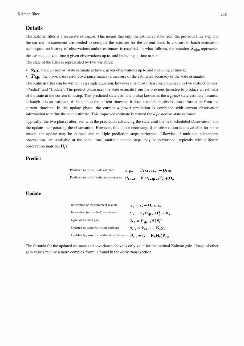
Kalman filter 238
DetailsThe Kalman filter is a recursive estimator. This means that only the estimated state from the previous time step andthe current measurement are needed to compute the estimate for the current state. In contrast to batch estimationtechniques, no history of observations and/or estimates is required. In what follows, the notation representsthe estimate of at time n given observations up to, and including at time m ≤ n.The state of the filter is represented by two variables:
• , the a posteriori state estimate at time k given observations up to and including at time k;• , the a posteriori error covariance matrix (a measure of the estimated accuracy of the state estimate).The Kalman filter can be written as a single equation, however it is most often conceptualized as two distinct phases:"Predict" and "Update". The predict phase uses the state estimate from the previous timestep to produce an estimateof the state at the current timestep. This predicted state estimate is also known as the a priori state estimate because,although it is an estimate of the state at the current timestep, it does not include observation information from thecurrent timestep. In the update phase, the current a priori prediction is combined with current observationinformation to refine the state estimate. This improved estimate is termed the a posteriori state estimate.Typically, the two phases alternate, with the prediction advancing the state until the next scheduled observation, andthe update incorporating the observation. However, this is not necessary; if an observation is unavailable for somereason, the update may be skipped and multiple prediction steps performed. Likewise, if multiple independentobservations are available at the same time, multiple update steps may be performed (typically with differentobservation matrices Hk).
Predict
Predicted (a priori) state estimate
Predicted (a priori) estimate covariance
Update
Innovation or measurement residual
Innovation (or residual) covariance
Optimal Kalman gain
Updated (a posteriori) state estimate
Updated (a posteriori) estimate covariance
The formula for the updated estimate and covariance above is only valid for the optimal Kalman gain. Usage of othergain values require a more complex formula found in the derivations section.
Kalman filter 239
Invariants
If the model is accurate, and the values for and accurately reflect the distribution of the initial statevalues, then the following invariants are preserved: (all estimates have a mean error of zero)••where is the expected value of , and covariance matrices accurately reflect the covariance of estimates•••
Estimation of the noise covariances Qk and RkPractical implementation of the Kalman Filter is often difficult due to the inability in getting a good estimate of thenoise covariance matrices Qk and Rk. Extensive research has been done in this field to estimate these covariancesfrom data. One of the more promising approaches to do this is the Autocovariance Least-Squares (ALS) techniquethat uses autocovariances of routine operating data to estimate the covariances.[9][10] The GNU Octave code used tocalculate the noise covariance matrices using the ALS technique is available online under the GNU General PublicLicense license.
Optimality and performanceIt is known from the theory that the Kalman filter is optimal in case that a) the model perfectly matches the realsystem, b) the entering noise is white and c) the covariances of the noise are exactly known. Several methods for thenoise covariance estimation have been proposed during past decades. One, ALS, was mentioned in the previousparagraph. After the covariances are identified, it is useful to evaluate the performance of the filter, i.e. whether it ispossible to improve the state estimation quality. It is well known that, if the Kalman filter works optimally, theinnovation sequence (the output prediction error) is a white noise. The whiteness property reflects the stateestimation quality. For evaluation of the filter performance it is necessary to inspect the whiteness property of theinnovations. Several different methods can be used for this purpose. Three optimality tests with numerical examplesare described in [11]
Example application, technicalConsider a truck on perfectly frictionless, infinitely long straight rails. Initially the truck is stationary at position 0,but it is buffeted this way and that by random acceleration. We measure the position of the truck every Δt seconds,but these measurements are imprecise; we want to maintain a model of where the truck is and what its velocity is.We show here how we derive the model from which we create our Kalman filter.Since F, H, R and Q are constant, their time indices are dropped.The position and velocity of the truck are described by the linear state space
where is the velocity, that is, the derivative of position with respect to time.We assume that between the (k−1) and k timestep the truck undergoes a constant acceleration of ak that is normallydistributed, with mean 0 and standard deviation σa. From Newton's laws of motion we conclude that
(note that there is no term since we have no known control inputs) where
Kalman filter 240
and
so that
where and
At each time step, a noisy measurement of the true position of the truck is made. Let us suppose the measurementnoise vk is also normally distributed, with mean 0 and standard deviation σz.
where
and
We know the initial starting state of the truck with perfect precision, so we initialize
and to tell the filter that we know the exact position, we give it a zero covariance matrix:
If the initial position and velocity are not known perfectly the covariance matrix should be initialized with a suitablylarge number, say L, on its diagonal.
The filter will then prefer the information from the first measurements over the information already in the model.
Derivations
Deriving the a posteriori estimate covariance matrixStarting with our invariant on the error covariance Pk | k as above
substitute in the definition of
and substitute
and
and by collecting the error vectors we get
Kalman filter 241
Since the measurement error vk is uncorrelated with the other terms, this becomes
by the properties of vector covariance this becomes
which, using our invariant on Pk | k−1 and the definition of Rk becomes
This formula (sometimes known as the "Joseph form" of the covariance update equation) is valid for any value ofKk. It turns out that if Kk is the optimal Kalman gain, this can be simplified further as shown below.
Kalman gain derivationThe Kalman filter is a minimum mean-square error estimator. The error in the a posteriori state estimation is
We seek to minimize the expected value of the square of the magnitude of this vector, . This isequivalent to minimizing the trace of the a posteriori estimate covariance matrix . By expanding out the termsin the equation above and collecting, we get:
The trace is minimized when its matrix derivative with respect to the gain matrix is zero. Using the gradient matrixrules and the symmetry of the matrices involved we find that
Solving this for Kk yields the Kalman gain:
This gain, which is known as the optimal Kalman gain, is the one that yields MMSE estimates when used.
Simplification of the a posteriori error covariance formulaThe formula used to calculate the a posteriori error covariance can be simplified when the Kalman gain equals theoptimal value derived above. Multiplying both sides of our Kalman gain formula on the right by SkKk
T, it followsthat
Referring back to our expanded formula for the a posteriori error covariance,
we find the last two terms cancel out, giving
This formula is computationally cheaper and thus nearly always used in practice, but is only correct for the optimalgain. If arithmetic precision is unusually low causing problems with numerical stability, or if a non-optimal Kalmangain is deliberately used, this simplification cannot be applied; the a posteriori error covariance formula as derivedabove must be used.
Kalman filter 242
Sensitivity analysisThe Kalman filtering equations provide an estimate of the state and its error covariance recursively. Theestimate and its quality depend on the system parameters and the noise statistics fed as inputs to the estimator. Thissection analyzes the effect of uncertainties in the statistical inputs to the filter. In the absence of reliable statistics orthe true values of noise covariance matrices and , the expression
no longer provides the actual error covariance. In other words, . In mostreal time applications the covariance matrices that are used in designing the Kalman filter are different from theactual noise covariances matrices.Wikipedia:Citation needed This sensitivity analysis describes the behavior of theestimation error covariance when the noise covariances as well as the system matrices and that are fed asinputs to the filter are incorrect. Thus, the sensitivity analysis describes the robustness (or sensitivity) of theestimator to misspecified statistical and parametric inputs to the estimator.This discussion is limited to the error sensitivity analysis for the case of statistical uncertainties. Here the actual noisecovariances are denoted by and respectively, whereas the design values used in the estimator are and
respectively. The actual error covariance is denoted by and as computed by the Kalman filter isreferred to as the Riccati variable. When and , this means that . Whilecomputing the actual error covariance using , substituting for and
using the fact that and , results in the following recursive equations for:
and
While computing , by design the filter implicitly assumes that and .Note that the recursive expressions for and are identical except for the presence of and inplace of the design values and respectively.
Square root formOne problem with the Kalman filter is its numerical stability. If the process noise covariance Qk is small, round-offerror often causes a small positive eigenvalue to be computed as a negative number. This renders the numericalrepresentation of the state covariance matrix P indefinite, while its true form is positive-definite.Positive definite matrices have the property that they have a triangular matrix square root P = S·ST. This can becomputed efficiently using the Cholesky factorization algorithm, but more importantly, if the covariance is kept inthis form, it can never have a negative diagonal or become asymmetric. An equivalent form, which avoids many ofthe square root operations required by the matrix square root yet preserves the desirable numerical properties, is theU-D decomposition form, P = U·D·UT, where U is a unit triangular matrix (with unit diagonal), and D is a diagonalmatrix.Between the two, the U-D factorization uses the same amount of storage, and somewhat less computation, and is themost commonly used square root form. (Early literature on the relative efficiency is somewhat misleading, as itassumed that square roots were much more time-consuming than divisions,:69 while on 21-st century computers theyare only slightly more expensive.)Efficient algorithms for the Kalman prediction and update steps in the square root form were developed by G. J.Bierman and C. L. Thornton.The L·D·LT decomposition of the innovation covariance matrix Sk is the basis for another type of numerically efficient and robust square root filter. The algorithm starts with the LU decomposition as implemented in the Linear
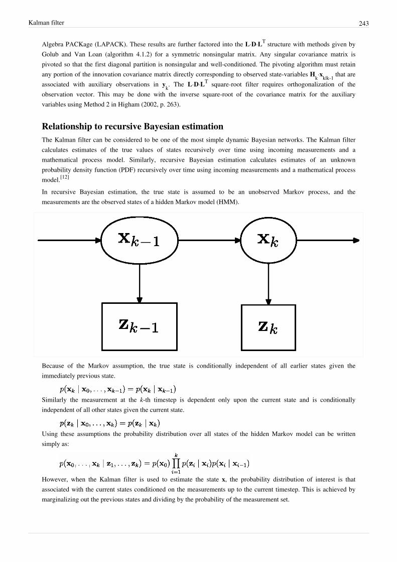
Kalman filter 243
Algebra PACKage (LAPACK). These results are further factored into the L·D·LT structure with methods given byGolub and Van Loan (algorithm 4.1.2) for a symmetric nonsingular matrix. Any singular covariance matrix ispivoted so that the first diagonal partition is nonsingular and well-conditioned. The pivoting algorithm must retainany portion of the innovation covariance matrix directly corresponding to observed state-variables Hk·xk|k-1 that areassociated with auxiliary observations in yk. The L·D·LT square-root filter requires orthogonalization of theobservation vector. This may be done with the inverse square-root of the covariance matrix for the auxiliaryvariables using Method 2 in Higham (2002, p. 263).
Relationship to recursive Bayesian estimationThe Kalman filter can be considered to be one of the most simple dynamic Bayesian networks. The Kalman filtercalculates estimates of the true values of states recursively over time using incoming measurements and amathematical process model. Similarly, recursive Bayesian estimation calculates estimates of an unknownprobability density function (PDF) recursively over time using incoming measurements and a mathematical processmodel.[12]
In recursive Bayesian estimation, the true state is assumed to be an unobserved Markov process, and themeasurements are the observed states of a hidden Markov model (HMM).
Because of the Markov assumption, the true state is conditionally independent of all earlier states given theimmediately previous state.
Similarly the measurement at the k-th timestep is dependent only upon the current state and is conditionallyindependent of all other states given the current state.
Using these assumptions the probability distribution over all states of the hidden Markov model can be writtensimply as:
However, when the Kalman filter is used to estimate the state x, the probability distribution of interest is thatassociated with the current states conditioned on the measurements up to the current timestep. This is achieved bymarginalizing out the previous states and dividing by the probability of the measurement set.

Kalman filter 244
This leads to the predict and update steps of the Kalman filter written probabilistically. The probability distributionassociated with the predicted state is the sum (integral) of the products of the probability distribution associated withthe transition from the (k − 1)-th timestep to the k-th and the probability distribution associated with the previousstate, over all possible .
The measurement set up to time t is
The probability distribution of the update is proportional to the product of the measurement likelihood and thepredicted state.
The denominator
is a normalization term.The remaining probability density functions are
Note that the PDF at the previous timestep is inductively assumed to be the estimated state and covariance. This isjustified because, as an optimal estimator, the Kalman filter makes best use of the measurements, therefore the PDFfor given the measurements is the Kalman filter estimate.
Information filterIn the information filter, or inverse covariance filter, the estimated covariance and estimated state are replaced by theinformation matrix and information vector respectively. These are defined as:
Similarly the predicted covariance and state have equivalent information forms, defined as:
as have the measurement covariance and measurement vector, which are defined as:
The information update now becomes a trivial sum.
The main advantage of the information filter is that N measurements can be filtered at each timestep simply bysumming their information matrices and vectors.
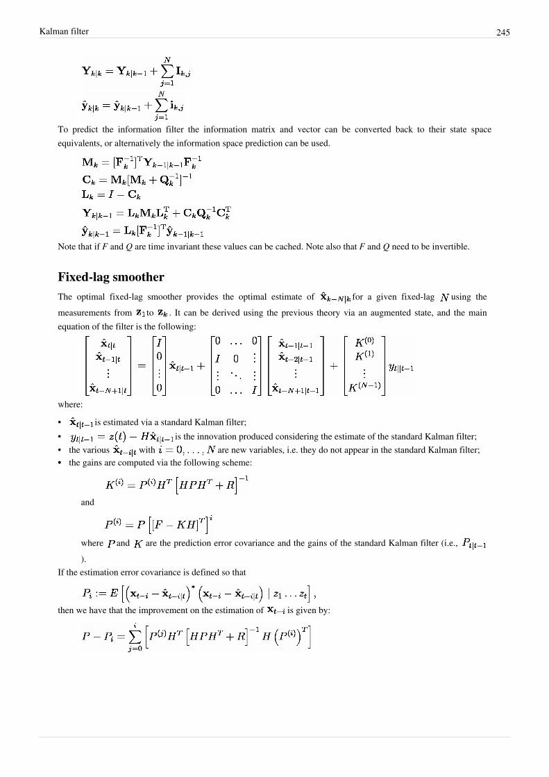
Kalman filter 245
To predict the information filter the information matrix and vector can be converted back to their state spaceequivalents, or alternatively the information space prediction can be used.
Note that if F and Q are time invariant these values can be cached. Note also that F and Q need to be invertible.
Fixed-lag smootherThe optimal fixed-lag smoother provides the optimal estimate of for a given fixed-lag using themeasurements from to . It can be derived using the previous theory via an augmented state, and the mainequation of the filter is the following:
where:
• is estimated via a standard Kalman filter;• is the innovation produced considering the estimate of the standard Kalman filter;• the various with are new variables, i.e. they do not appear in the standard Kalman filter;•• the gains are computed via the following scheme:
and
where and are the prediction error covariance and the gains of the standard Kalman filter (i.e., ).
If the estimation error covariance is defined so that
then we have that the improvement on the estimation of is given by:
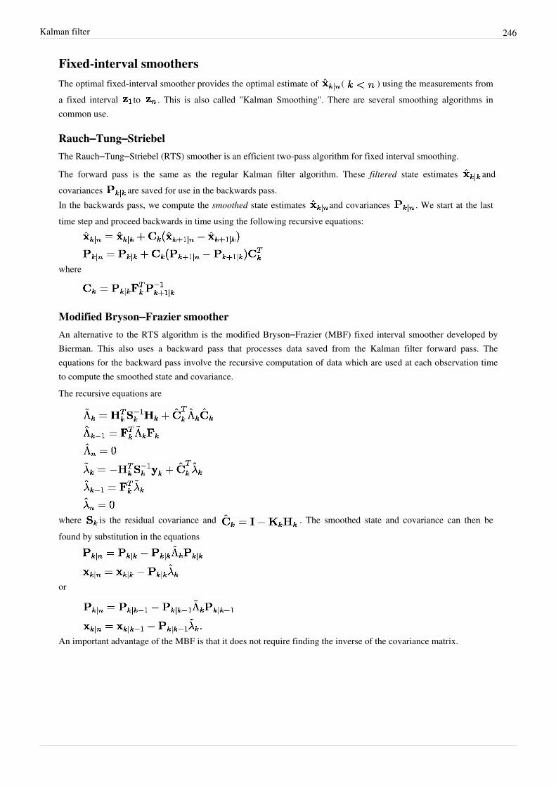
Kalman filter 246
Fixed-interval smoothersThe optimal fixed-interval smoother provides the optimal estimate of ( ) using the measurements froma fixed interval to . This is also called "Kalman Smoothing". There are several smoothing algorithms incommon use.
Rauch–Tung–StriebelThe Rauch–Tung–Striebel (RTS) smoother is an efficient two-pass algorithm for fixed interval smoothing.
The forward pass is the same as the regular Kalman filter algorithm. These filtered state estimates andcovariances are saved for use in the backwards pass.In the backwards pass, we compute the smoothed state estimates and covariances . We start at the lasttime step and proceed backwards in time using the following recursive equations:
where
Modified Bryson–Frazier smootherAn alternative to the RTS algorithm is the modified Bryson–Frazier (MBF) fixed interval smoother developed byBierman. This also uses a backward pass that processes data saved from the Kalman filter forward pass. Theequations for the backward pass involve the recursive computation of data which are used at each observation timeto compute the smoothed state and covariance.The recursive equations are
where is the residual covariance and . The smoothed state and covariance can then befound by substitution in the equations
or
An important advantage of the MBF is that it does not require finding the inverse of the covariance matrix.

Kalman filter 247
Minimum-variance smootherThe minimum-variance smoother can attain the best-possible error performance, provided that the models are linear,their parameters and the noise statistics are known precisely. This smoother is a time-varying state-spacegeneralization of the optimal non-causal Wiener filter.The smoother calculations are done in two passes. The forward calculations involve a one-step-ahead predictor andare given by
The above system is known as the inverse Wiener-Hopf factor. The backward recursion is the adjoint of the aboveforward system. The result of the backward pass may be calculated by operating the forward equations on thetime-reversed and time reversing the result. In the case of output estimation, the smoothed estimate is given by
Taking the causal part of this minimum-variance smoother yields
which is identical to the minimum-variance Kalman filter. The above solutions minimize the variance of the outputestimation error. Note that the Rauch–Tung–Striebel smoother derivation assumes that the underlying distributionsare Gaussian, whereas the minimum-variance solutions do not. Optimal smoothers for state estimation and inputestimation can be constructed similarly.A continuous-time version of the above smoother is described in.Expectation-maximization algorithms may be employed to calculate approximate maximum likelihood estimates ofunknown state-space parameters within minimum-variance filters and smoothers. Often uncertainties remain withinproblem assumptions. A smoother that accommodates uncertainties can be designed by adding a positive definiteterm to the Riccati equation.In cases where the models are nonlinear, step-wise linearizations may be within the minimum-variance filter andsmoother recursions (Extended Kalman filtering).
Non-linear filtersThe basic Kalman filter is limited to a linear assumption. More complex systems, however, can be nonlinear. Thenon-linearity can be associated either with the process model or with the observation model or with both.
Extended Kalman filterMain article: Extended Kalman filterIn the extended Kalman filter (EKF), the state transition and observation models need not be linear functions of thestate but may instead be non-linear functions. These functions are of differentiable type.
The function f can be used to compute the predicted state from the previous estimate and similarly the function h canbe used to compute the predicted measurement from the predicted state. However, f and h cannot be applied to thecovariance directly. Instead a matrix of partial derivatives (the Jacobian) is computed.At each timestep the Jacobian is evaluated with current predicted states. These matrices can be used in the Kalmanfilter equations. This process essentially linearizes the non-linear function around the current estimate.

Kalman filter 248
Unscented Kalman filter
When the state transition and observation models—that is, the predict and update functions and —are highlynon-linear, the extended Kalman filter can give particularly poor performance. This is because the covariance ispropagated through linearization of the underlying non-linear model. The unscented Kalman filter (UKF) uses adeterministic sampling technique known as the unscented transform to pick a minimal set of sample points (calledsigma points) around the mean. These sigma points are then propagated through the non-linear functions, fromwhich the mean and covariance of the estimate are then recovered. The result is a filter which more accuratelycaptures the true mean and covariance. (This can be verified using Monte Carlo sampling or through a Taylor seriesexpansion of the posterior statistics.) In addition, this technique removes the requirement to explicitly calculateJacobians, which for complex functions can be a difficult task in itself (i.e., requiring complicated derivatives if doneanalytically or being computationally costly if done numerically).PredictAs with the EKF, the UKF prediction can be used independently from the UKF update, in combination with a linear(or indeed EKF) update, or vice versa.The estimated state and covariance are augmented with the mean and covariance of the process noise.
A set of 2L + 1 sigma points is derived from the augmented state and covariance where L is the dimension of thestate.
where
is the ith column of the matrix square root of
using the definition: square root A of matrix B satisfies
The matrix square root should be calculated using numerically efficient and stable methods such as the Choleskydecomposition.The sigma points are propagated through the transition function f.
where . The weighted sigma points are recombined to produce the predicted state and covariance.
where the weights for the state and covariance are given by:

Kalman filter 249
and control the spread of the sigma points. is related to the distribution of . Normal values are, and . If the true distribution of is Gaussian, is optimal.[13]
UpdateThe predicted state and covariance are augmented as before, except now with the mean and covariance of themeasurement noise.
As before, a set of 2L + 1 sigma points is derived from the augmented state and covariance where L is the dimensionof the state.
Alternatively if the UKF prediction has been used the sigma points themselves can be augmented along thefollowing lines
where
The sigma points are projected through the observation function h.
The weighted sigma points are recombined to produce the predicted measurement and predicted measurementcovariance.
The state-measurement cross-covariance matrix,
is used to compute the UKF Kalman gain.

Kalman filter 250
As with the Kalman filter, the updated state is the predicted state plus the innovation weighted by the Kalman gain,
And the updated covariance is the predicted covariance, minus the predicted measurement covariance, weighted bythe Kalman gain.
Kalman–Bucy filterThe Kalman–Bucy filter (named after Richard Snowden Bucy) is a continuous time version of the Kalmanfilter.[14][15]
It is based on the state space model
where and represent the intensities of the two white noise terms and , respectively.The filter consists of two differential equations, one for the state estimate and one for the covariance:
where the Kalman gain is given by
Note that in this expression for the covariance of the observation noise represents at the same time thecovariance of the prediction error (or innovation) ; these covariances are equal only inthe case of continuous time.[16]
The distinction between the prediction and update steps of discrete-time Kalman filtering does not exist incontinuous time.The second differential equation, for the covariance, is an example of a Riccati equation.
Hybrid Kalman filterMost physical systems are represented as continuous-time models while discrete-time measurements are frequentlytaken for state estimation via a digital processor. Therefore, the system model and measurement model are given by
where
.Initialize
Predict
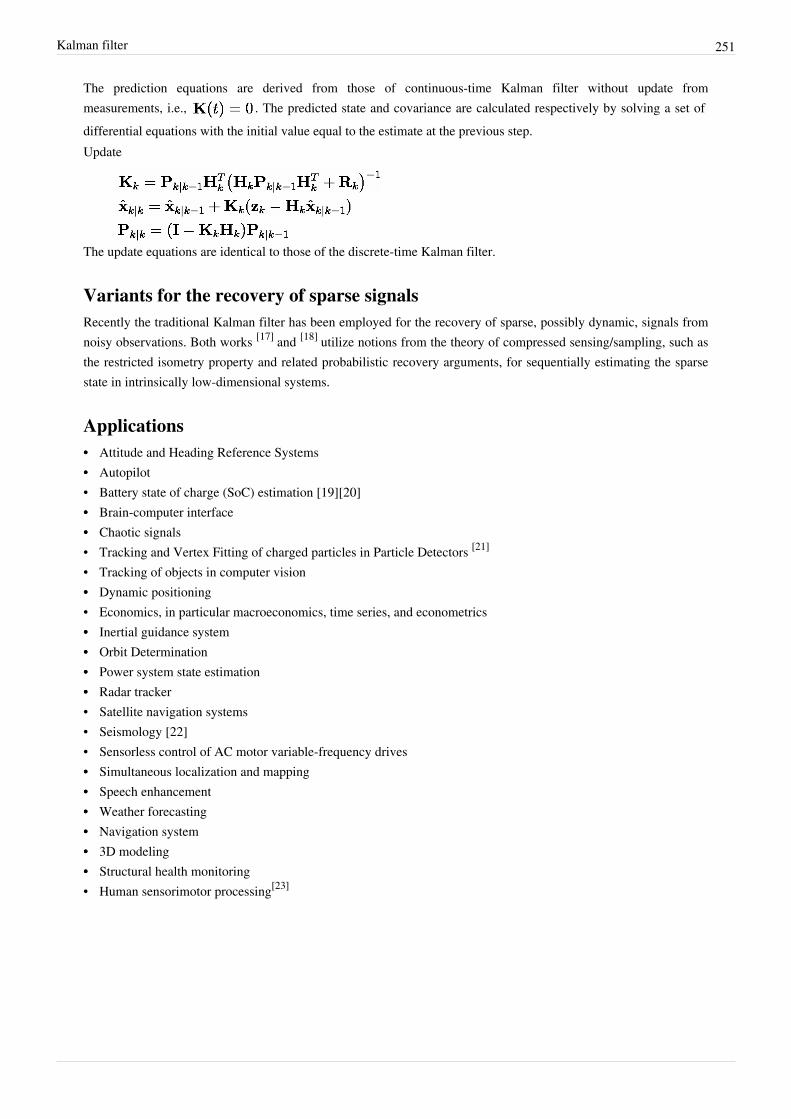
Kalman filter 251
The prediction equations are derived from those of continuous-time Kalman filter without update frommeasurements, i.e., . The predicted state and covariance are calculated respectively by solving a set ofdifferential equations with the initial value equal to the estimate at the previous step.Update
The update equations are identical to those of the discrete-time Kalman filter.
Variants for the recovery of sparse signalsRecently the traditional Kalman filter has been employed for the recovery of sparse, possibly dynamic, signals fromnoisy observations. Both works [17] and [18] utilize notions from the theory of compressed sensing/sampling, such asthe restricted isometry property and related probabilistic recovery arguments, for sequentially estimating the sparsestate in intrinsically low-dimensional systems.
Applications•• Attitude and Heading Reference Systems•• Autopilot• Battery state of charge (SoC) estimation [19][20]•• Brain-computer interface•• Chaotic signals• Tracking and Vertex Fitting of charged particles in Particle Detectors [21]
• Tracking of objects in computer vision•• Dynamic positioning• Economics, in particular macroeconomics, time series, and econometrics•• Inertial guidance system•• Orbit Determination•• Power system state estimation•• Radar tracker• Satellite navigation systems• Seismology [22]• Sensorless control of AC motor variable-frequency drives•• Simultaneous localization and mapping•• Speech enhancement•• Weather forecasting•• Navigation system•• 3D modeling•• Structural health monitoring• Human sensorimotor processing[23]
Kalman filter 252
References[1] Steffen L. Lauritzen (http:/ / www. stats. ox. ac. uk/ ~steffen/ ). "Time series analysis in 1880. A discussion of contributions made by T.N.
Thiele". International Statistical Review 49, 1981, 319–333.[2] Steffen L. Lauritzen, Thiele: Pioneer in Statistics (http:/ / www. oup. com/ uk/ catalogue/ ?ci=9780198509721), Oxford University Press,
2002. ISBN 0-19-850972-3.[3] Stratonovich, R.L. (1959). Optimum nonlinear systems which bring about a separation of a signal with constant parameters from noise.
Radiofizika, 2:6, pp. 892–901.[4] Stratonovich, R.L. (1959). On the theory of optimal non-linear filtering of random functions. Theory of Probability and its Applications, 4,
pp. 223–225.[5] Stratonovich, R.L. (1960) Application of the Markov processes theory to optimal filtering. Radio Engineering and Electronic Physics, 5:11,
pp. 1–19.[6] Stratonovich, R.L. (1960). Conditional Markov Processes. Theory of Probability and its Applications, 5, pp. 156–178.[7] Roweis, S. and Ghahramani, Z., A unifying review of linear Gaussian models (http:/ / www. mitpressjournals. org/ doi/ abs/ 10. 1162/
089976699300016674), Neural Comput. Vol. 11, No. 2, (February 1999), pp. 305–345.[8] Hamilton, J. (1994), Time Series Analysis, Princeton University Press. Chapter 13, 'The Kalman Filter'.[9] "Rajamani, Murali – PhD Thesis" (http:/ / jbrwww. che. wisc. edu/ theses/ rajamani. pdf) Data-based Techniques to Improve State Estimation
in Model Predictive Control, University of Wisconsin-Madison, October 2007[10] Rajamani, Murali R. and Rawlings, James B., Estimation of the disturbance structure from data using semidefinite programming and
optimal weighting. Automatica, 45:142–148, 2009.[11][11] Matisko P. and V. Havlena (2012). Optimality tests and adaptive Kalman filter. Proceedings of 16th IFAC System Identification
Symposium, Brussels, Belgium.[12] C. Johan Masreliez, R D Martin (1977); Robust Bayesian estimation for the linear model and robustifying the Kalman filter (http:/ /
ieeexplore. ieee. org/ xpl/ freeabs_all. jsp?arnumber=1101538), IEEE Trans. Automatic Control[13] Wan, Eric A. and van der Merwe, Rudolph "The Unscented Kalman Filter for Nonlinear Estimation" (http:/ / www. lara. unb. br/ ~gaborges/
disciplinas/ efe/ papers/ wan2000. pdf)[14] Bucy, R.S. and Joseph, P.D., Filtering for Stochastic Processes with Applications to Guidance, John Wiley & Sons, 1968; 2nd Edition,
AMS Chelsea Publ., 2005. ISBN 0-8218-3782-6[15] Jazwinski, Andrew H., Stochastic processes and filtering theory, Academic Press, New York, 1970. ISBN 0-12-381550-9[16] Kailath, Thomas, "An innovation approach to least-squares estimation Part I: Linear filtering in additive white noise", IEEE Transactions on
Automatic Control, 13(6), 646-655, 1968[17] Carmi, A. and Gurfil, P. and Kanevsky, D. , "Methods for sparse signal recovery using Kalman filtering with embedded
pseudo-measurement norms and quasi-norms", IEEE Transactions on Signal Processing, 58(4), 2405–2409, 2010[18] Vaswani, N. , "Kalman Filtered Compressed Sensing", 15th International Conference on Image Processing, 2008[19] http:/ / dx. doi. org/ 10. 1016/ j. jpowsour. 2007. 04. 011[20] http:/ / dx. doi. org/ 10. 1016/ j. enconman. 2007. 05. 017[21][21] Nucl.Instrum.Meth. A262 (1987) 444-450. Application of Kalman filtering to track and vertex fitting. R. Fruhwirth (Vienna, OAW).[22] http:/ / adsabs. harvard. edu/ abs/ 2008AGUFM. G43B. . 01B[23] Neural Netw. 1996 Nov;9(8):1265–1279. Forward Models for Physiological Motor Control. Wolpert DM, Miall RC.
Further reading• Einicke, G.A. (2012). Smoothing, Filtering and Prediction: Estimating the Past, Present and Future (http:/ /
www. intechopen. com/ books/ smoothing-filtering-and-prediction-estimating-the-past-present-and-future).Rijeka, Croatia: Intech. ISBN 978-953-307-752-9.
• Gelb, A. (1974). Applied Optimal Estimation. MIT Press.• Kalman, R.E. (1960). "A new approach to linear filtering and prediction problems" (http:/ / www. elo. utfsm. cl/
~ipd481/ Papers varios/ kalman1960. pdf). Journal of Basic Engineering 82 (1): 35–45. doi: 10.1115/1.3662552(http:/ / dx. doi. org/ 10. 1115/ 1. 3662552). Retrieved 2008-05-03.
• Kalman, R.E.; Bucy, R.S. (1961). New Results in Linear Filtering and Prediction Theory (http:/ / www. dtic. mil/srch/ doc?collection=t2& id=ADD518892). Retrieved 2008-05-03.Wikipedia:Link rot
• Harvey, A.C. (1990). Forecasting, Structural Time Series Models and the Kalman Filter. Cambridge UniversityPress.
• Roweis, S.; Ghahramani, Z. (1999). "A Unifying Review of Linear Gaussian Models". Neural Computation 11(2): 305–345. doi: 10.1162/089976699300016674 (http:/ / dx. doi. org/ 10. 1162/ 089976699300016674). PMID 9950734 (http:/ / www. ncbi. nlm. nih. gov/ pubmed/ 9950734).

Kalman filter 253
• Simon, D. (2006). Optimal State Estimation: Kalman, H Infinity, and Nonlinear Approaches (http:/ / academic.csuohio. edu/ simond/ estimation/ ). Wiley-Interscience.
• Stengel, R.F. (1994). Optimal Control and Estimation (http:/ / www. princeton. edu/ ~stengel/ OptConEst. html).Dover Publications. ISBN 0-486-68200-5.
• Warwick, K. (1987). "Optimal observers for ARMA models" (http:/ / www. informaworld. com/ index/779885789. pdf). International Journal of Control 46 (5): 1493–1503. doi: 10.1080/00207178708933989 (http:/ /dx. doi. org/ 10. 1080/ 00207178708933989). Retrieved 2008-05-03.
• Bierman, G.J. (1977). "Factorization Methods for Discrete Sequential Estimation". Mathematics in Science andEngineering 128 (Mineola, N.Y.: Dover Publications). ISBN 978-0-486-44981-4.
• Bozic, S.M. (1994). Digital and Kalman filtering. Butterworth–Heinemann.• Haykin, S. (2002). Adaptive Filter Theory. Prentice Hall.• Liu, W.; Principe, J.C. and Haykin, S. (2010). Kernel Adaptive Filtering: A Comprehensive Introduction. John
Wiley.• Manolakis, D.G. (1999). Statistical and Adaptive signal processing. Artech House.• Welch, Greg; Bishop, Gary (1997). "SCAAT" (http:/ / www. cs. unc. edu/ ~welch/ media/ pdf/ scaat. pdf).
SCAAT: Incremental Tracking with Incomplete Information. ACM Press/Addison-Wesley Publishing Co.pp. 333–344. doi: 10.1145/258734.258876 (http:/ / dx. doi. org/ 10. 1145/ 258734. 258876).ISBN 0-89791-896-7.
• Jazwinski, Andrew H. (1970). Stochastic Processes and Filtering. Mathematics in Science and Engineering. NewYork: Academic Press. p. 376. ISBN 0-12-381550-9.
• Maybeck, Peter S. (1979). Stochastic Models, Estimation, and Control. Mathematics in Science and Engineering.141-1. New York: Academic Press. p. 423. ISBN 0-12-480701-1.
• Moriya, N. (2011). Primer to Kalman Filtering: A Physicist Perspective. New York: Nova Science Publishers,Inc. ISBN 978-1-61668-311-5.
• Dunik, J.; Simandl M., Straka O. (2009). "Methods for estimating state and measurement noise covariancematrices: Aspects and comparisons". Proceedings of 15th IFAC Symposium on System Identification (France):372–377.
• Chui, Charles K.; Chen, Guanrong (2009). Kalman Filtering with Real-Time Applications. Springer Series inInformation Sciences 17 (4th ed.). New York: Springer. p. 229. ISBN 978-3-540-87848-3.
• Spivey, Ben; Hedengren, J. D. and Edgar, T. F. (2010). "Constrained Nonlinear Estimation for Industrial ProcessFouling" (http:/ / pubs. acs. org/ doi/ abs/ 10. 1021/ ie9018116). Industrial & Engineering Chemistry Research 49(17): 7824–7831. doi: 10.1021/ie9018116 (http:/ / dx. doi. org/ 10. 1021/ ie9018116).
• Thomas Kailath, Ali H. Sayed, and Babak Hassibi, Linear Estimation, Prentice–Hall, NJ, 2000, ISBN978-0-13-022464-4.
• Ali H. Sayed, Adaptive Filters, Wiley, NJ, 2008, ISBN 978-0-470-25388-5.
External links• A New Approach to Linear Filtering and Prediction Problems (http:/ / www. cs. unc. edu/ ~welch/ kalman/
kalmanPaper. html), by R. E. Kalman, 1960• Kalman–Bucy Filter (http:/ / www. eng. tau. ac. il/ ~liptser/ lectures1/ lect6. pdf), a good derivation of the
Kalman–Bucy Filter• MIT Video Lecture on the Kalman filter (https:/ / www. youtube. com/ watch?v=d0D3VwBh5UQ) on YouTube• An Introduction to the Kalman Filter (http:/ / www. cs. unc. edu/ ~tracker/ media/ pdf/
SIGGRAPH2001_CoursePack_08. pdf), SIGGRAPH 2001 Course, Greg Welch and Gary Bishop• Kalman filtering chapter (http:/ / www. cs. unc. edu/ ~welch/ kalman/ media/ pdf/ maybeck_ch1. pdf) from
Stochastic Models, Estimation, and Control, vol. 1, by Peter S. Maybeck• Kalman Filter (http:/ / www. cs. unc. edu/ ~welch/ kalman/ ) webpage, with lots of links

Kalman filter 254
• "Kalman Filtering" (https:/ / web. archive. org/ web/ 20130623214223/ http:/ / www. innovatia. com/ software/papers/ kalman. htm). Archived from the original (http:/ / www. innovatia. com/ software/ papers/ kalman. htm)on 2013-06-23.
• Kalman Filters, thorough introduction to several types, together with applications to Robot Localization (http:/ /www. negenborn. net/ kal_loc/ )
• Kalman filters used in Weather models (http:/ / www. siam. org/ pdf/ news/ 362. pdf), SIAM News, Volume 36,Number 8, October 2003.
• Critical Evaluation of Extended Kalman Filtering and Moving-Horizon Estimation (http:/ / pubs. acs. org/ cgi-bin/abstract. cgi/ iecred/ 2005/ 44/ i08/ abs/ ie034308l. html), Ind. Eng. Chem. Res., 44 (8), 2451–2460, 2005.
• Source code for the propeller microprocessor (http:/ / obex. parallax. com/ object/ 326): Well documented sourcecode written for the Parallax propeller processor.
• Gerald J. Bierman's Estimation Subroutine Library (http:/ / netlib. org/ a/ esl. tgz): Corresponds to the code in theresearch monograph "Factorization Methods for Discrete Sequential Estimation" originally published byAcademic Press in 1977. Republished by Dover.
• Matlab Toolbox implementing parts of Gerald J. Bierman's Estimation Subroutine Library (http:/ / www.mathworks. com/ matlabcentral/ fileexchange/ 32537): UD / UDU' and LD / LDL' factorization with associatedtime and measurement updates making up the Kalman filter.
• Matlab Toolbox of Kalman Filtering applied to Simultaneous Localization and Mapping (http:/ / eia. udg. es/~qsalvi/ Slam. zip): Vehicle moving in 1D, 2D and 3D
• Derivation of a 6D EKF solution to Simultaneous Localization and Mapping (http:/ / www. mrpt. org/ 6D-SLAM)(In old version PDF (http:/ / mapir. isa. uma. es/ ~jlblanco/ papers/ RangeBearingSLAM6D. pdf)). See also thetutorial on implementing a Kalman Filter (http:/ / www. mrpt. org/ Kalman_Filters) with the MRPT C++ libraries.
• The Kalman Filter Explained (http:/ / www. tristanfletcher. co. uk/ LDS. pdf) A very simple tutorial.• The Kalman Filter in Reproducing Kernel Hilbert Spaces (http:/ / www. cnel. ufl. edu/ ~weifeng/ publication.
htm) A comprehensive introduction.• Matlab code to estimate Cox–Ingersoll–Ross interest rate model with Kalman Filter (http:/ / www. mathfinance.
cn/ kalman-filter-finance-revisited/ ): Corresponds to the paper "estimating and testing exponential-affine termstructure models by kalman filter" published by Review of Quantitative Finance and Accounting in 1999.
• Extended Kalman Filters (http:/ / apmonitor. com/ wiki/ index. php/ Main/ Background) explained in the contextof Simulation, Estimation, Control, and Optimization
• Online demo of the Kalman Filter (http:/ / www. data-assimilation. net/ Tools/ AssimDemo/ ?method=KF).Demonstration of Kalman Filter (and other data assimilation methods) using twin experiments.
• Handling noisy environments: the k-NN delta s, on-line adaptive filter. (http:/ / dx. doi. org/ 10. 3390/s110808164) in Robust high performance reinforcement learning through weighted k-nearest neighbors,Neurocomputing, 74(8), March 2011, pp. 1251–1259.
• Hookes Law and the Kalman Filter (http:/ / finmathblog. blogspot. com/ 2013/ 10/hookes-law-and-kalman-filter-little. html) A little "spring theory" emphasizing the connection between statisticsand physics.
• Examples and how-to on using Kalman Filters with MATLAB (http:/ / www. mathworks. com/ discovery/kalman-filter. html)

Wiener filter 255
Wiener filterIn signal processing, the Wiener filter is a filter used to produce an estimate of a desired or target random processby linear time-invariant filtering an observed noisy process, assuming known stationary signal and noise spectra, andadditive noise. The Wiener filter minimizes the mean square error between the estimated random process and thedesired process.
Application of the Wiener filter for noise suppression. Left: original image; middle:image with added noise; right: filtered image
Description
The goal of the Wiener filter is to filterout noise that has corrupted a signal. Itis based on a statistical approach, and amore statistical account of the theory isgiven in the MMSE estimator article.
Typical filters are designed for adesired frequency response. However,the design of the Wiener filter takes adifferent approach. One is assumed to have knowledge of the spectral properties of the original signal and the noise,and one seeks the linear time-invariant filter whose output would come as close to the original signal as possible.Wiener filters are characterized by the following:
1. Assumption: signal and (additive) noise are stationary linear stochastic processes with known spectralcharacteristics or known autocorrelation and cross-correlation
2. Requirement: the filter must be physically realizable/causal (this requirement can be dropped, resulting in anon-causal solution)
3. Performance criterion: minimum mean-square error (MMSE)This filter is frequently used in the process of deconvolution; for this application, see Wiener deconvolution.
Wiener filter problem setupThe input to the Wiener filter is assumed to be a signal, , corrupted by additive noise, . The output, , is calculated by means of a filter, , using the following convolution:
where is the original signal (not exactly known; to be estimated), is the noise, is the estimatedsignal (the intention is to equal ), and is the Wiener filter's impulse response.The error is defined as
where is the delay of the Wiener Filter (since it is causal). In other words, the error is the difference between theestimated signal and the true signal shifted by .The squared error is
where is the desired output of the filter and is the error. Depending on the value of , theproblem can be described as follows:• if then the problem is that of prediction (error is reduced when is similar to a later value of s),
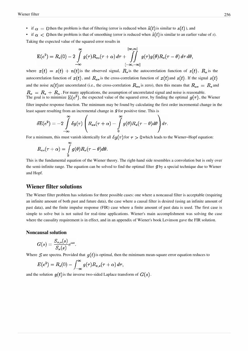
Wiener filter 256
• if then the problem is that of filtering (error is reduced when is similar to ), and• if then the problem is that of smoothing (error is reduced when is similar to an earlier value of s).Taking the expected value of the squared error results in
where is the observed signal, is the autocorrelation function of , is theautocorrelation function of , and is the cross-correlation function of and . If the signal and the noise are uncorrelated (i.e., the cross-correlation is zero), then this means that and
. For many applications, the assumption of uncorrelated signal and noise is reasonable.The goal is to minimize , the expected value of the squared error, by finding the optimal , the Wienerfilter impulse response function. The minimum may be found by calculating the first order incremental change in theleast square resulting from an incremental change in for positive time. This is
For a minimum, this must vanish identically for all for which leads to the Wiener–Hopf equation:
This is the fundamental equation of the Wiener theory. The right-hand side resembles a convolution but is only overthe semi-infinite range. The equation can be solved to find the optimal filter by a special technique due to Wienerand Hopf.
Wiener filter solutionsThe Wiener filter problem has solutions for three possible cases: one where a noncausal filter is acceptable (requiringan infinite amount of both past and future data), the case where a causal filter is desired (using an infinite amount ofpast data), and the finite impulse response (FIR) case where a finite amount of past data is used. The first case issimple to solve but is not suited for real-time applications. Wiener's main accomplishment was solving the casewhere the causality requirement is in effect, and in an appendix of Wiener's book Levinson gave the FIR solution.
Noncausal solution
Where are spectra. Provided that is optimal, then the minimum mean-square error equation reduces to
and the solution is the inverse two-sided Laplace transform of .
Wiener filter 257
Causal solution
where
• consists of the causal part of (that is, that part of this fraction having a positive time solution
under the inverse Laplace transform)• is the causal component of (i.e., the inverse Laplace transform of is non-zero only for
)• is the anti-causal component of (i.e., the inverse Laplace transform of is non-zero only
for )This general formula is complicated and deserves a more detailed explanation. To write down the solution ina specific case, one should follow these steps:1. Start with the spectrum in rational form and factor it into causal and anti-causal components:
where contains all the zeros and poles in the left half plane (LHP) and contains the zeroes and poles inthe right half plane (RHP). This is called the Wiener–Hopf factorization.
2. Divide by and write out the result as a partial fraction expansion.3. Select only those terms in this expansion having poles in the LHP. Call these terms .4. Divide by . The result is the desired filter transfer function .
Finite impulse response Wiener filter for discrete series
Block diagram view of the FIR Wiener filter for discrete series. An input signal w[n] isconvolved with the Wiener filter g[n] and the result is compared to a reference signal s[n]
to obtain the filtering error e[n].
The causal finite impulse response(FIR) Wiener filter, instead of usingsome given data matrix X and outputvector Y, finds optimal tap weights byusing the statistics of the input andoutput signals. It populates the inputmatrix X with estimates of theauto-correlation of the input signal (T)and populates the output vector Y withestimates of the cross-correlationbetween the output and input signals (V).
In order to derive the coefficients of the Wiener filter, consider the signal w[n] being fed to a Wiener filter of order Nand with coefficients , . The output of the filter is denoted x[n] which is given by theexpression
The residual error is denoted e[n] and is defined as e[n] = x[n] − s[n] (see the corresponding block diagram). TheWiener filter is designed so as to minimize the mean square error (MMSE criteria) which can be stated concisely asfollows:
where denotes the expectation operator. In the general case, the coefficients may be complex and may be derived for the case where w[n] and s[n] are complex as well. With a complex signal, the matrix to be solved is a

Wiener filter 258
Hermitian Toeplitz matrix, rather than symmetric Toeplitz matrix. For simplicity, the following considers only thecase where all these quantities are real. The mean square error (MSE) may be rewritten as:
To find the vector which minimizes the expression above, calculate its derivative with respect to
Assuming that w[n] and s[n] are each stationary and jointly stationary, the sequences and knownrespectively as the autocorrelation of w[n] and the cross-correlation between w[n] and s[n] can be defined as follows:
The derivative of the MSE may therefore be rewritten as (notice that )
Letting the derivative be equal to zero results in
which can be rewritten in matrix form
These equations are known as the Wiener–Hopf equations. The matrix T appearing in the equation is a symmetricToeplitz matrix. Under suitable conditions on , these matrices are known to be positive definite and thereforenon-singular yielding a unique solution to the determination of the Wiener filter coefficient vector, .Furthermore, there exists an efficient algorithm to solve such Wiener–Hopf equations known as the Levinson-Durbinalgorithm so an explicit inversion of is not required.
Relationship to the least mean squares filterThe realization of the causal Wiener filter looks a lot like the solution to the least squares estimate, except in thesignal processing domain. The least squares solution, for input matrix and output vector is
The FIR Wiener filter is related to the least mean squares filter, but minimizing the error criterion of the latter doesnot rely on cross-correlations or auto-correlations. Its solution converges to the Wiener filter solution.

Wiener filter 259
ApplicationsThe Wiener filter can be used in image processing to remove noise from a picture. For example, using theMathematica function: WienerFilter[image,2] on the first image on the right, produces the filtered imagebelow it.
Noisy image of astronaut.
Noisy image of astronaut after Wiener filterapplied.
It is commonly used to denoise audio signals, especially speech, as apreprocessor before speech recognition.
History
The filter was proposed by Norbert Wiener during the 1940s andpublished in 1949. The discrete-time equivalent of Wiener's work wasderived independently by Andrey Kolmogorov and published in 1941.Hence the theory is often called the Wiener–Kolmogorov filteringtheory. The Wiener filter was the first statistically designed filter to beproposed and subsequently gave rise to many others including thefamous Kalman filter.
References
• Thomas Kailath, Ali H. Sayed, and Babak Hassibi, LinearEstimation, Prentice-Hall, NJ, 2000, ISBN 978-0-13-022464-4.
•• Wiener N: The interpolation, extrapolation and smoothing ofstationary time series', Report of the Services 19, Research ProjectDIC-6037 MIT, February 1942
• Kolmogorov A.N: 'Stationary sequences in Hilbert space', (In Russian) Bull. Moscow Univ. 1941 vol.2 no.6 1-40.English translation in Kailath T. (ed.) Linear least squares estimation Dowden, Hutchinson & Ross 1977
External links• Mathematica WienerFilter (http:/ / reference. wolfram. com/ mathematica/ ref/ WienerFilter. html) function

260
Receivers
Article Sources and Contributors 261
Article Sources and ContributorsDigital signal processing Source: http://en.wikipedia.org/w/index.php?oldid=608654794 Contributors: .:Ajvol:., 3dB dar, A.amitkumar, Abdul muqeet, Abdull, Adoniscik, AeroPsico, Agasta,Alberto Orlandini, Alinja, Allen4names, Allstarecho, Alphachimp, Andy M. Wang, AndyThe, Ap, Arta1365, Atlant, AxelBoldt, Bact, Belizefan, Ben-Zin, Betacommand, Binksternet, BoleslavBobcik, Bongwarrior, Brion VIBBER, CLW, Caiaffa, Can't sleep, clown will eat me, CapitalR, Captain-tucker, Cburnett, Cgrislin, Chinneeb, ChrisGualtieri, Coneslayer, Conversion script, Cst17,Ctmt, Cybercobra, Cyberparam, DARTH SIDIOUS 2, DJS, Dawdler, Dicklyon, Discospinster, Dr Alan Hewitt, Dreadstar, Drew335, Ds13, Dspanalyst, Dysprosia, Eart4493, Easterbrook,EmadIV, Epbr123, ErrantX, Essjay, Excirial, Fgnievinski, Fieldday-sunday, Finlay McWalter, Frmatt, Furrykef, Gbuffett, Ged Davies, GeorgeBarnick, Gfoltz9, Giftlite, Gimboid13, Glenn, Glrx,Graham87, Greglocock, Gökhan, HelgeStenstrom, Helwr, Hezarfenn, Hooperbloob, Hu12, Humourmind, Hyacinth, Indeterminate, Inductiveload, Iquinnm, Isarra (HG), JPushkarH, JackGreenmaven, Jeancey, Jefchip, Jeff8080, Jehochman, Jeremyp1988, Jmrowland, Jnothman, Joaopchagas2, Jogfalls1947, JohnPritchard, Johnpseudo, Johnuniq, Jondel, Josve05a, Jshadias,Kesaloma, King Lopez, Kku, Kurykh, Kvng, LCS check, Landen99, Ldo, LilHelpa, Loisel, Lzur, MER-C, Mac, Martpol, Materialscientist, Matt Britt, Mcapdevila, Mdd4696, Mesoderm, MichaelHardy, MightCould, Mistman123, Moberg, Mohammed hameed, Moxfyre, Mutaza, Mwilde, Mysid, Niceguyedc, Nixdorf, Nvd, OSP Editor, Ohnoitsjamie, Olivier, Omegatron, Omeomi, Onehalf 3544, Orange Suede Sofa, OrgasGirl, PEHowland, Paileboat, Pantech solutions, Patrick, Pdfpdf, Pgan002, Phoebe, Physicsch, Pinkadelica, Prari, Raanoo, Rade Kutil, Radiodef, Rbj,Recurring dreams, Refikh, Rememberway, RexNL, Reza1615, Rickyrazz, Rogueleaderr, Rohan2kool, RomanSpa, Ronz, SWAdair, SamShearman, Sandeeppasala, Savidan, Semitransgenic, SethNimbosa, ShashClp, Shekure, Siddharth raw, Sisyphus110, Skarebo, SkiAustria, Smack, Soumyasch, SpaceFlight89, Spectrogram, Stan Sykora, Stevebillings, Stillastillsfan, Striznauss, Style,Swagato Barman Roy, Tbackstr, Tcs az, Tertiary7, The Anome, The Photon, Thebestofall007, Thisara.d.m, Tobias Hoevekamp, Togo, Tomer Ish Shalom, Tony Sidaway, Tot12, Travelingseth,Trlkly, Trolleymusic, Turgan, TutterMouse, Ukexpat, Van helsing, Vanished user 34958, Vermolaev, Versus22, Vinras, Violetriga, Vizcarra, VladimirDsp, Wayne Hardman, Webclient101,Webshared, Whoop whoop, Wknight8111, Wolfkeeper, Ww, Y(J)S, Yangjy0113, Yaroslavvb, Yewyew66, Yswismer, Zvika, 397 anonymous edits
Discrete signal Source: http://en.wikipedia.org/w/index.php?oldid=568050497 Contributors: AK456, Artyom, Axel.hallinder, Bob K, Cburnett, Dicklyon, Dreadstar, Duoduoduo, Fjarlq,Hamamelis, Krishnavedala, Lambiam, Longhair, Marius, Meteor sandwich yum, Michael Hardy, Olli Niemitalo, Omegatron, Petr.adamek, Pol098, Radiodef, Rbj, Rinconsoleao, Ring0, Rs2,ShashClp, Smack, Soun0786, Spinningspark, Tow, Unschool, Vasiľ, Vina, Walton One, Wdwd, Xezbeth, 40 anonymous edits
Sampling (signal processing) Source: http://en.wikipedia.org/w/index.php?oldid=611650993 Contributors: ANDROBETA, Adoniscik, Andres, Anna Frodesiak, Barking Mad42, Binksternet,Bjbarman18, Bob K, BorgQueen, Chemako0606, Chris the speller, Colonies Chris, ContinueWithCaution, Cosmin1595, DaBler, Dan Polansky, DavidCary, Deineka, Dicklyon, Edcolins,Email4mobile, Epbr123, Fgnievinski, Gene Nygaard, Gggbgggb, Giftlite, Gionnico, Heron, Hongthay, ImEditingWiki, Infvwl, JLaTondre, JaGa, Jan Arkesteijn, Jheald, Jim1138, Jk2q3jrklse,John Holmes II, Joz3d, JulienBourdon, Kimchi.sg, Kjoonlee, Kvng, LilHelpa, Lorem Ip, LutzL, MagnusA, Mattbr, Meteor sandwich yum, Miym, Mnkmnkmnk990, Nanren888, Nbarth, Neøn,Oleg Alexandrov, OverlordQ, Patriarch, Philip Trueman, Physicsch, Pvosta, Rami R, Ravn, Rbj, Rcunderw, ScotXW, Selket, Shantham11, Sigmundg, Smack, Soliloquial, Sowndaryab,Spinningspark, StefanosNikolaou, Teapeat, Thiseye, Trusilver, Txomin, Unused0022, VanishedUserABC, Webclient101, Wolfkeeper, Zvika, 133 anonymous edits
Sample and hold Source: http://en.wikipedia.org/w/index.php?oldid=583548339 Contributors: Adoniscik, Arnero, BBCLCD, Bachrach44, Bpromo7, Cburnett, Cheezwzl, Ciphers,David.Monniaux, Deville, Donald Albury, East of Borschov, Fluffernutter, Foobaz, GRAHAMUK, Gareth Griffith-Jones, Gdilla, Hooperbloob, Hut 8.5, Jaiswalrita, Koavf, Lv131, Magioladitis,Mange01, Mattisse, Mdrejhon, Menswear, Michael Hardy, MikeWazowski, Mitchan, Mjb, Ring0, Riumplus, Rjwilmsi, Se cicret, SiegeLord, SoledadKabocha, Strake, Tabletop, Thedatastream,Timrprobocom, Tswsl1989, Udaysagarpanjala, Vikrant More14, VoiceEncoder, 42 anonymous edits
Digital-to-analog converter Source: http://en.wikipedia.org/w/index.php?oldid=602163327 Contributors: 10metreh, Abuthayar, Adamantios, Alansohn, Algocu, Analogkidr, Anaxial,Andrebragareis, Andy M. Wang, Arnero, BD2412, Bemoeial, BenFrantzDale, Binglau, Binksternet, Blitzmut, Bobrayner, Boodidha sampath, Bookandcoffee, Bpromo7, Bradeos Graphon,Brainmedley, BrianWilloughby, CPES, Calltech, Camyoung54, CanisRufus, Cburnett, Chad.Farmer, ChardonnayNimeque, Chepry, Chester Markel, Chmod007, Crm123, CryptoDerk, Cst17,DJS, Damian Yerrick, DanteLectro, Dept of Alchemy, Ecclaim, EncMstr, Father Goose, Fnfd, GRAHAMUK, Garion96, Giftlite, Glaisher, Glenn, Gradulov, Hellisp, HenkeB, Heron,Hooperbloob, Ht1848, Hugh Mason, ICE77, Imroy, Incminister, Jannev, Jeff3000, Joe Decker, John Siau, Johnteslade, JonHarder, Josvanehv, Karkat-H-NJITWILL, Kenyon, Kizor, Kvng, LeeCarre, Lexusuns, Lsuff, Lupo, Mahira75249, Mandarax, Masgatotkaca, Materialscientist, Maximus Rex, Mcleodm, Meestaplu, Michael Hardy, Mjb, Mortense, MrOllie, Nczempin, Neildmartin,Nono64, Ojigiri, Omegatron, Ontarioboy, Overjive, Paul August, Photonique, PierreAbbat, Pointillist, R'n'B, Ravenmewtwo, Rbj, Reddi, Redheylin, Rivertorch, RobinK, Rpal143, SWAdair,Salgueiro, Semiwiki, Sicaspi, Southcaltree, Spinningspark, Ssd, Stevenalex, StormtrooperTK421, StradivariusTV, Sturm br, TakuyaMurata, TedPavlic, Tex23, Thane, Tharanath1981, TheAnome, TheAMmollusc, Thue, Timecop, Topbanana, Travelingseth, UVnet, VQuakr, Waveguy, Wernher, Wolfkeeper, Woohookitty, Wsko.ko, Xx521xx, Yoshm, Zoicon5, 297 anonymous edits
Analog-to-digital converter Source: http://en.wikipedia.org/w/index.php?oldid=608380390 Contributors: 08Peter15, 28421u2232nfenfcenc, 4johnny, A4, AK456, Ablewisuk, Adoniscik,Adpete, AeroPsico, Ahoerstemeier, Alansohn, Ali Esfandiari, Alison22, Alll, Altenmann, Alvin Seville, Alvin-cs, Americanhero, Analogkidr, Andres, Anitauky, Arnab1984, Arnero,BenFrantzDale, BernardH, Berrinkursun, Bgwhite, Bhimaji, Binglau, Binksternet, Biscuittin, Blowfishie, Bob K, Bpromo7, BrianWilloughby, Brianga, Brisvegas, CambridgeBayWeather,CanisRufus, Cat5nap, ChardonnayNimeque, Charles Matthews, Chepry, Chetvorno, Chris the speller, ChrisGualtieri, Christian way, Cindy141, ClickRick, Cmdrjameson, Colin Marquardt,Coppertwig, Crohnie, Crystalllized, Csk, Cullen kasunic, Cutler, D4g0thur, DJS, Damian Yerrick, David Underdown, DavidCary, Davidkazuhiro, Davidmeo, Dayewalker, Dcirovic, DeadTotoro,Derek Ross, Dhiraj1984, Drpickem, Dufekin, EdSaWiki, Electron9, Ellmist, EncMstr, Erislover, Erynofwales, EthanL, Everyking, Evice, FakingNovember, Febert, Fgnievinski, Fmltavares,GRAHAMUK, Garion96, Gayanmyte, Gbalasandeep, Gene Nygaard, Giftlite, Gilliam, Gillsandeep2k, Ginsengbomb, Glrx, Goudzovski, GyroMagician, Hadal, Haikupoet, Heddmj, Hellisp,Heron, Hooperbloob, Hu12, ICE77, Iverson2, Ivnryn, Ixfd64, J.delanoy, Jahoe, Jan1nad, Jaxl, Jeff3000, Jerome Charles Potts, Jheiv, Jimi75, Jkominek, Jleedev, JohnTechnologist, Johnteslade,JonHarder, Josecampos, Jusdafax, Juxo, Kaleem str, Keegan, Klo, KnowledgeOfSelf, Kooo, Krishfeelmylove, Kvng, LeaveSleaves, Legend Saber, LilHelpa, LittleOldMe, Lmatt, MER-C,MR7526, Male1979, Materialscientist, Mbell, Mblumber, Mcleodm, Mecanismo, Meggar, Michael Hardy, Micru, MinorContributor, Mortense, MrOllie, Msadaghd, MusikAnimal, Nacho Insular,Nayuki, Nbarth, Neil.steiner, Nelbs, Nemilar, Nick C, Night Goblin, Nrpickle, Nsaa, Nwerneck, Ojigiri, Oli Filth, Omegatron, Overjive, Overmanic, Pavan206, Perry chesterfield, Peteraisher,Pietrow, Pjacobi, Purgatory Fubar, Qllach, Radiodef, Raka99, Rassom anatol, Redheylin, Reinderien, Requestion, Ring0, RobinK, Romanski, Roscoe x, STHayden, Samurai meatwad,Sandpiper800, SapnaArun, Satan131984, Saxbryn, Sbeath, Schickaneder, Scientizzle, Sciurinæ, Scottr9, Sfan00 IMG, Shaddack, Shadowjams, Shalabh24, Shawn81, Sicaspi, Sjbfalchion,Smurfettekla, Snoyes, Solarra, Sonett72, Southcaltree, Sparkie82, Spinningspark, Steven Zhang, Stevenj, Stigwall, Syl1729, Talkstosocks, Tbackstr, Teapeat, TecABC, Techeditor1, Tehtennisman, TheAMmollusc, Themfromspace, Theo177, Theslaw, Thue, Timrprobocom, Tjwikipedia, Travelingseth, Tristanb, Tslocum, Ttmartin2888, UkPaolo, VanishedUserABC, Vayalir,Virrisho001, VoidLurker, Wakebrdkid, Welsh, Wernher, Whiteflye, Wiki libs, Wikihitech, Windforce1989, Wolfkeeper, Wsmarz, Wtshymanski, Xorx, Yoshm, Yyy, Zipcube, Zootboy,Zueignung, 583 anonymous edits
Window function Source: http://en.wikipedia.org/w/index.php?oldid=611931547 Contributors: AGRAK, Abdull, Aervanath, Alberto Orlandini, Alejo2083, Aleks.labuda, Aquegg, Art LaPella,Bob K, BobQQ, Brad7777, Chadernook, Charles Matthews, ChiCheng, Chochopk, Conquerist, DavidCary, Dcljr, Debejyo, Dicklyon, Drizzd, Dysprosia, Ebmi, Ed g2s, EffeX2, Falcorian,Fgnievinski, Frecklefoot, Freezing in Wisconsin, Furrykef, Gasfet, Giftlite, Glenn, Glrx, GregorB, Guaka, GuenterRote, Haleyang, Heron, Illia Connell, Isheden, Jamesjyu, Japanese Searobin,Jimgeorge, Jinma, Joelthelion, Jorend, Jorge Stolfi, Jpkotta, KSmrq, Kevmitch, Kogge, Kvng, Lewallen, Light current, Luegge, MOBle, Macrakis, Magioladitis, Marcel Müller, Mark Arsten,Martianxo, MattieTK, Mecanismo, Mekonto, Melcombe, Michael Hardy, Mile10com, MrZebra, Mwtoews, Nbarth, Nicoguaro, Nmnogueira, Oleg Alexandrov, Oli Filth, Olli Niemitalo,Omegatron, Opt8236, Oxymoron83, PTT, PhilKnight, Quenhitran, Quibik, Rbarreira, Rjwilmsi, Rtbehrens, Safulop, Sandycx, Sangwine, SchreiberBike, Smcbuet, Soshial, Srleffler, StaticGull,Stevenj, Strebe, Suvo ganguli, Thunderbird2, Tiaguito, Unyoyega, Virens, Vit-net, Wavelength, WaywardGeek, Wikichicheng, Zom-B, Лъчезар, 267 anonymous edits
Quantization (signal processing) Source: http://en.wikipedia.org/w/index.php?oldid=607396892 Contributors: Aadri, BarrelProof, Beetelbug, BenFrantzDale, Bob K, Bulser, C xong, Cat5nap,Cburnett, Charles Matthews, Chris the speller, Constant314, DeadTotoro, DmitriyV, DopefishJustin, Engelec, Fernando.iglesiasg, Fgnievinski, Frze, Giftlite, Glenn, Gruauder, Hadiyana,Hyacinth, Itayperl, JordiTost, Kashyap.cherukuri, Khazar2, Kku, Krash, Kvng, Longhair, Matt Gies, Mblumber, Metacomet, Michael Hardy, Mobeets, Nayuki, Nbarth, Necromancer44, Oarih,Omegatron, OverlordQ, Pak21, Paolo.dL, Petr.adamek, Pol098, Radagast83, Radiodef, Rbj, RedWolf, RomanSpa, Rushbugled13, Sapphic, Shmlchr, Slady, Smack, SudoMonas, Sylenius, TheAnome, The Seventh Taylor, Topbanana, VanishedUserABC, Wdwd, WhiteHatLurker, 102 anonymous edits
Quantization error Source: http://en.wikipedia.org/w/index.php?oldid=555799903 Contributors: Aadri, BarrelProof, Beetelbug, BenFrantzDale, Bob K, Bulser, C xong, Cat5nap, Cburnett,Charles Matthews, Chris the speller, Constant314, DeadTotoro, DmitriyV, DopefishJustin, Engelec, Fernando.iglesiasg, Fgnievinski, Frze, Giftlite, Glenn, Gruauder, Hadiyana, Hyacinth, Itayperl,JordiTost, Kashyap.cherukuri, Khazar2, Kku, Krash, Kvng, Longhair, Matt Gies, Mblumber, Metacomet, Michael Hardy, Mobeets, Nayuki, Nbarth, Necromancer44, Oarih, Omegatron,OverlordQ, Pak21, Paolo.dL, Petr.adamek, Pol098, Radagast83, Radiodef, Rbj, RedWolf, RomanSpa, Rushbugled13, Sapphic, Shmlchr, Slady, Smack, SudoMonas, Sylenius, The Anome, TheSeventh Taylor, Topbanana, VanishedUserABC, Wdwd, WhiteHatLurker, 102 anonymous edits
ENOB Source: http://en.wikipedia.org/w/index.php?oldid=459141510 Contributors: Amalas, Belchman, Cs-wolves, DexDor, Elonka, Gene Nygaard, Glrx, GyroMagician, HelgeStenstrom,Heron, Jddriessen, Kvng, Lavaka, Malcolma, MarSch, Qwerty1234321, Radiodef, Rjwilmsi, Robofish, TedPavlic, Whpq, Zocky, Володимир Груша, 16 anonymous edits
Sampling rate Source: http://en.wikipedia.org/w/index.php?oldid=599589778 Contributors: ANDROBETA, Adoniscik, Andres, Anna Frodesiak, Barking Mad42, Binksternet, Bjbarman18, Bob K, BorgQueen, Chemako0606, Chris the speller, Colonies Chris, ContinueWithCaution, Cosmin1595, DaBler, Dan Polansky, DavidCary, Deineka, Dicklyon, Edcolins, Email4mobile, Epbr123, Fgnievinski, Gene Nygaard, Gggbgggb, Giftlite, Gionnico, Heron, Hongthay, ImEditingWiki, Infvwl, JLaTondre, JaGa, Jan Arkesteijn, Jheald, Jim1138, Jk2q3jrklse, John Holmes II, Joz3d, JulienBourdon, Kimchi.sg, Kjoonlee, Kvng, LilHelpa, Lorem Ip, LutzL, MagnusA, Mattbr, Meteor sandwich yum, Miym, Mnkmnkmnk990, Nanren888, Nbarth, Neøn, Oleg Alexandrov,
Article Sources and Contributors 262
OverlordQ, Patriarch, Philip Trueman, Physicsch, Pvosta, Rami R, Ravn, Rbj, Rcunderw, ScotXW, Selket, Shantham11, Sigmundg, Smack, Soliloquial, Sowndaryab, Spinningspark,StefanosNikolaou, Teapeat, Thiseye, Trusilver, Txomin, Unused0022, VanishedUserABC, Webclient101, Wolfkeeper, Zvika, 133 anonymous edits
Nyquist–Shannon sampling theorem Source: http://en.wikipedia.org/w/index.php?oldid=610791098 Contributors: .:Ajvol:., 195.149.37.xxx, 24.7.91.xxx, A4, Acdx, Ash, AxelBoldt, BD2412,Barraki, Bdmy, BenFrantzDale, Bender235, BeteNoir, Bob K, Brad7777, Brion VIBBER, Cabe6403, Camembert, Cameronc, Cblambert, Cburnett, Cihan, Coderzombie, Colonies Chris,Conversion script, CosineKitty, Courcelles, Cryptonaut, DARTH SIDIOUS 2, Damian Yerrick, Dbagnall, Default007, Deodar, Dicklyon, DigitalPhase, Dougmcgeehan, Drhex, Duagloth,Dysprosia, Editor at Large, Enochlau, Enormator, ErickOrtiz, Fang Aili, Finell, First Harmonic, Fleem, Floatjon, Frazzydee, Gah4, Gaius Cornelius, Geekmug, Gene Nygaard, Giftlite, Graham87,Heron, Hogno, Hongthay, Hrafn, Hu12, Humourmind, Ian Pitchford, IanOfNorwich, IgorCarron, IstvanWolf, Jac16888, Jacobolus, Jannex, Jasón, Jesse Viviano, Jheald, Jim1138, Jncraton,Juansempere, KYN, Karn, Kbrose, Kenyon, Ketil3, Krash, Kvng, Larry Sanger, Lavaka, LenoreMarks, Liangjingjin, Ligand, Light current, Lightmouse, Loisel, LouScheffer, Lovibond,Lowellian, Lupin, LutzL, M4701, Maansi.t, Maghnus, Mange01, Manscher, Marcoracer, Mav, Mboverload, Mct mht, Metacomet, Mets501, Michael Hardy, Michaelmestre, Minochang, Miym,Movado73, Mperrin, Mrand, Mwilde, Nafeun, Nbarth, Neckro, Niteowlneils, Nuwewsco, Oddbodz, Odo Benus, Oli Filth, Omegatron, Oskar Sigvardsson, Ost316, OverlordQ, Patrick, Perelaar,Pfalstad, Phil Boswell, PhotoBox, Pr103, Psychonaut, Pvosta, Qef, Quondum, RAE, RDBury, RTBoyce, Rbj, Rednectar.chris, Reedy, Robert K S, Sam Hocevar, Sander123, Sawf,SciCompTeacher, SebastianHelm, Shantham11, Shelbymoore3, Skittleys, SlimDeli, Slipstream, Smack, Solarapex, Stefoo, Stupefaction, Teapeat, TedPavlic, The Thing That Should Not Be,Thenub314, Tiddly Tom, Tomas e, Tompagenet, TooComplicated, TriciaMcmillian, Waveguy, Wavelength, Wolfkeeper, X-Fi6, Ytw1987, ZeroOne, Zueignung, Zundark, Zvika, 321 ,יובל מדרanonymous edits
Nyquist frequency Source: http://en.wikipedia.org/w/index.php?oldid=611382787 Contributors: Alblupo, Andrerogers21, Ardonik, Bob K, Boldone, Cannolis, Cburnett, ChrisGualtieri,CosineKitty, Dewritech, Dicklyon, Diegotorquemada, Dtcdthingy, Dysprosia, El C, Eloquence, Etimbo, Fgnievinski, Foogus, Giftlite, Glenn, Hariva, HatlessAtlas, Heron, Jonesey95, JoshCherry, K6ka, Katieh5584, Kiefer.Wolfowitz, Kri, Magioladitis, Mange01, MarXidad, Materialscientist, Metacomet, Nbarth, OhGodItsSoAmazing, Oldmaneinstein, Oli Filth, Orange Suede Sofa,Parijata, Physicsch, Pvosta, Rbj, Spinningspark, Stevenj, Stuver, SvBiker, Tassedethe, Tene, The Anome, TreeSmiler, Wolfmankurd, Wpkelley, 65 anonymous edits
Nyquist rate Source: http://en.wikipedia.org/w/index.php?oldid=600273959 Contributors: Alinja, BenFrantzDale, Bob K, BorzouBarzegar, Cburnett, Dicklyon, EconoPhysicist, Editor at Large,Encambio, Gaius Cornelius, Giftlite, HatlessAtlas, Heron, Jangirke, Mange01, Metacomet, Michael Hardy, Oli Filth, Parijata, Rbj, Rdrosson, Rjwilmsi, Rosuna, Scarfboy, SebastianHelm, Sepiatone, Tarotcards, The Thing That Should Not Be, User A1, Wdwd, Widr, 27 anonymous edits
Oversampling Source: http://en.wikipedia.org/w/index.php?oldid=603963355 Contributors: AJRussell, ANDROBETA, Adam McMaster, Adityaip, Alager, AndyHe829, Benzi455, CIreland,Cantaloupe2, Cburnett, Charles Matthews, CosineKitty, Deville, Dicklyon, DisillusionedBitterAndKnackered, Duagloth, Elg fr, Estudente, Furrykef, Gcc111, Giftlite, Gregfitzy, Ice Cold Beer,Irishguy, Isidore, Kvng, Ldo, Mblumber, Myasuda, Mysid, Nick Number, Omegatron, R'n'B, Radiodef, Rakeshmisra, Rbj, Rogerbrent, Sayeed shaik, SebastianHelm, Shlomital, Snorgy, St3vo,Swazi Radar, TYonley, Thorney¿?, Titodutta, Urnonav, [email protected], Welsh, Winterstein, 63 anonymous edits
Undersampling Source: http://en.wikipedia.org/w/index.php?oldid=607207001 Contributors: ANDROBETA, Bob K, Dicklyon, Hooperbloob, J.delanoy, Mange01, Nbarth, Pawinsync,Psychonaut, 9 anonymous edits
Delta-sigma modulation Source: http://en.wikipedia.org/w/index.php?oldid=608212922 Contributors: 121a0012, Alain r, Alistair1978, Altzinn, Andy Dingley, Atlant, Bappi48, Beetelbug, BobBermani, Bpromo7, Bratsche, CapitalR, Charles Matthews, Cojoco, CyrilB, Damian Yerrick, DavidCary, Denisarona, DmitTrix, Druzhnik, Edokter, Epugachev, Gaius Cornelius, Gerweck,GregorB, Gruauder, Hankwang, Hanspi, HenningThielemann, Icarus4586, Jab843, Jd8837, Jim.henderson, Jkl, Jwinius, Katanzag, Ketiltrout, Krishnavedala, Kvng, Lanugo, Lm317t, Lulo.it,Lv131, Mahira75249, Margin1522, Markhurd, Mblumber, Mild Bill Hiccup, Mortense, MrOllie, Muon, Mwarren us, NOW, Nummify, Officiallyover, Ohconfucius, Omegatron, Onionmon,Optimale, Ozfest, Puffingbilly, Qdr, Raj.rlb, ReidWender, Requestion, Rich Farmbrough, Rjf ie, Rjwilmsi, S Roper, Sam8, Sandro cello, Sanjosanjo, SchuminWeb, Serrano24, Skpreddy, Snood1,Southcaltree, StradivariusTV, Tchai, TedPavlic, Tetvesdugo, The Anome, Theking2, Voidxor, Wsmarz, Yates, 183 ,عبد المؤمن anonymous edits
Jitter Source: http://en.wikipedia.org/w/index.php?oldid=610303502 Contributors: -oo0(GoldTrader)0oo-, 28421u2232nfenfcenc, Alq131, Ancheta Wis, AntigonusPedia, Apshore, Attilios,Aulis Eskola, Axfangli, BORGATO Pierandrea, CYD, Cedar101, Chris the speller, Chscholz, Closedmouth, Colin Marquardt, Daichinger, Dcoetzee, Deville, DexDor, Djg2006, DocWatson42,DragonHawk, DragonflySixtyseven, Drbreznjev, EBorisch, Edcolins, Edward, Electron, Firefly322, Forenti, Fresheneesz, Geffmax, Ggiust, Giraffedata, Gracefool, Grammarmonger, Heron,JanCeuleers, Japanese Searobin, Jfilcik, Jim.henderson, John Siau, John of Reading, Johnaduley, JonHarder, Josh Parris, Jrmwng, Jtir, Ju66l3r, Jurgen Hissen, Kambaalayashwanth, Kbrose,Kvng, Kyonmelg, Lambtron, Lee Carre, Leizer, Lmatt, Lockeownzj00, MJ94, Mandramas, Mariagor, Markrpw, Matticus78, Mc6809e, Michael Hardy, Moreati, MrRavaz, Msebast, Nasa-verve,Nwk, Object01, Oddbodz, OlEnglish, Omegatron, Pissant, Postrach, Prolog, Reguiieee, Requestion, Rev3rend, Rich Farmbrough, Rjwilmsi, Rod57, Ross Fraser, Rpspeck, Rs2, Rurigok, SamHocevar, SarahKitty, Sideways713, Spinningspark, Stevenmyan, Stonehead, TechWriterNJ, Tevildo, Th4n3r, TheMandarin, Thoobik, Toffile, ToobMug, Transcend, Trevor MacInnis, Vinucube,Vydeoatpict, Wsmarz, Zawer, Zetawoof, 162 anonymous edits
Aliasing Source: http://en.wikipedia.org/w/index.php?oldid=604756201 Contributors: ANDROBETA, Ablewisuk, Aeons, Anomalocaris, Arconada, Arthurcburigo, Awotter, BD2412,BenFrantzDale, BernardH, Blacklemon67, Bob K, Bwmodular, Cburnett, Ccwelt, Chodorkovskiy, Cindy141, Closetsingle, Commander Keane, Dicklyon, Diftil, Dino, Dlincoln, DonDiego,Dude1818, Dysprosia, ENeville, Earcatching, ElectronicsEnthusiast, Eloquence, EnglishTea4me, Fgnievinski, Furrykef, GRAHAMUK, Gene Nygaard, Giftlite, Gopalkrishnan83, Grimey, Heron,Hfastedge, Hierarchivist, Hymek, Ike9898, Jamelan, Jeepday, Jorge Stolfi, Josh Cherry, JulesH, Kshieh, Kusma, Kvng, Leon math, Lmatt, Loisel, Lowellian, Martin Kozák, Mblumber, Mejbp,Michael Hardy, Morrowfolk, Moxfyre, Nbarth, Nova77, Oli Filth, Ost316, Patrick, Pawinsync, Phil Boswell, PolBr, RTC, Rbj, Reatlas, RedWolf, Revolving Bugbear, RexNL, Roadrunner,Robert P. O'Shea, Sade, Shanes, Simiprof, SlipperyHippo, Smack, Snoyes, Srittau, Ssola, Steel Wool Killer, Stevegrossman, Stevertigo, Stillwaterising, Straker, TAnthony, TaintedMustard,Teapeat, The Anome, Tlotoxl, Tom.Reding, Tomic, Verijax, Wapcaplet, WhiteOak2006, WikiSlasher, Wolfkeeper, Wsmarz, Zoicon5, عبد المؤمن, Ὁ οἶστρος, 158 anonymous edits
Anti-aliasing filter Source: http://en.wikipedia.org/w/index.php?oldid=611396473 Contributors: 121a0012, Aschauer, Binksternet, Cburnett, Chumbu, Clubwarez, CommonsDelinker, DARTHSIDIOUS 2, DavidLeighEllis, Deville, Dicklyon, Djayjp, Drake Wilson, Dratman, Giftlite, Gsarwa, H2g2bob, Hooperbloob, Jalo, Kvng, KymFarnik, Melonkelon, Michael Frind, Mirror Vax,Nbarth, Nicransby, Norrk, Omnicloud, Ost316, Poulpy, Redheylin, Sneak, Stevegrossman, The Anome, 30 anonymous edits
Flash ADC Source: http://en.wikipedia.org/w/index.php?oldid=583056010 Contributors: Bmearns, Bwpach, ChardonnayNimeque, EAderhold, ELLAPRISCI, Guerberj, Iridescent,Jim.henderson, JohnI, OpaPiloot, Overjive, Reelrt, Sharoneditha, Sherool, SlipperyHippo, Squids and Chips, Wdwd, Wsmarz, 26 anonymous edits
Successive approximation ADC Source: http://en.wikipedia.org/w/index.php?oldid=606437390 Contributors: Amalas, B Pete, BD2412, Biscuittin, Braincricket, Btyner, EAderhold, Ec5618,Eus Kevin, Ferdinand Pienaar, Firebat08, Jeff3000, LittleCreature, Mandarax, Michael Hardy, Nolelover, Oli Filth, Omar El-Sewefy, Pankaj Warule, Pjrm, R'n'B, Salvar, SeymourSycamore,Smyth, Tabletop, Whiteflye, Zeeyanwiki, 68 anonymous edits
Integrating ADC Source: http://en.wikipedia.org/w/index.php?oldid=580851064 Contributors: Bender235, Bootsup, Dolovis, ElPeste, Glrx, Iamchanged, Scottr9, Wdwd, Wtshymanski, 5anonymous edits
Time-stretch analog-to-digital converter Source: http://en.wikipedia.org/w/index.php?oldid=252768262 Contributors: Alifard, BD2412, Bjfwiki, Bwb1729, Chowbok, Dthomsen8, John ofReading, Kkmurray, Klemen Kocjancic, Mbell, Michael Hardy, PhnomPencil, Physchim62, R'n'B, Schmloof, Shalabh24, Spinningspark, The Anome, Tom.Reding, 24 anonymous edits
Discrete Fourier transform Source: http://en.wikipedia.org/w/index.php?oldid=611237758 Contributors: 1exec1, Abevac, Alberto Orlandini, Alexjs (usurped), AliceNovak, Arialblack, ArthurRubin, AsceticRose, Astronautics, AxelBoldt, BD2412, Ben.k.horner, Benhorsburgh, Bill411432, Blin00, Bmitov, Bo Jacoby, Bob K, Bob.v.R, Bongomatic, Booyabazooka, Borching, BryanDerksen, CRGreathouse, Cburnett, Centrx, Charles Matthews, ChrisGualtieri, ChrisRuvolo, Citizentoad, Connelly, Conversion script, CoolBlue1234, Crazyvas, Cuzkatzimhut, Cybedu,Cybercobra, Cyp, DBigXray, David R. Ingham, Davidmeo, Dcoetzee, Dicklyon, DmitTrix, DopefishJustin, DrBob, Dysprosia, Dzordzm, EconoPhysicist, Ed g2s, Edward, Emvee, Epolk,EverettColdwell, Fakufaku, Felipebm, Flyer22, Foobaz, Fru1tbat, Furrykef, Galaxiaad, Gareth Owen, Gauge, Gene Nygaard, Geoeg, Giftlite, Glogger, Graham87, GregRM, Gryllida, Hanspi,HappyCamper, Helwr, HenningThielemann, Herr Satz, Hesam7, Hobit, Humatronic, IMochi, Iyerkri, Java410, Jeenriquez, JeromeJerome, Jitse Niesen, Jorge Stolfi, Justin W Smith, Jwkuehne,Kohtala, Kompik, Kramer, Kvng, LMB, Linmanatee, Lockeownzj00, Loisel, LokiClock, Lorem Ip, Madmardigan53, Man It's So Loud In Here, Martynas Patasius, Maschen, MathMartin,Matithyahu, Mcclurmc, Mckee, Mdebets, Metacomet, Michael Hardy, MightyWarrior, MikeJ9919, Minesweeper, Minghong, Mjb, Mlibby, Msuzen, Mulligatawny, Nayuki, Nbarth, Nikai,Nitin.mehta, NormDor, Oleg Alexandrov, Oli Filth, Omegatron, OrgasGirl, Ospalh, Oyz, PAR, Pak21, Paul August, Paul Matthews, Peter Stalin, Pgimeno, Phil Boswell, Poslfit, Pseudomonas,Rabbanis, Rdrk, Recognizance, Robin S, Ronhjones, Saltine, Sam Hocevar, Sampletalk, Sbyrnes321, SebastianHelm, Shakeel3442, Sharpoo7, SheeEttin, Srleffler, Ssd, Stevenj, Sverdrup, Svick,Swagato Barman Roy, Tabletop, Tbackstr, The wub, TheMightyOrb, Thenub314, Thorwald, Tobias Bergemann, Uncia, Uncle Dick, User A1, Verdy p, Wavelength, Wbm1058, Welsh, Wikid77,Wile E. Heresiarch, Woohookitty, Zueignung, Zundark, Zvika, Zxcvbnm, Пика Пика, 291 anonymous edits
Fast Fourier transform Source: http://en.wikipedia.org/w/index.php?oldid=610645065 Contributors: 16@r, 2ganesh, Aclassifier, Adam Zivner, Adashiel, Akoesters, AliceNovak, Amitparikh, Apexfreak, Apteva, Artur Nowak, Audriusa, Avalcarce, AxelBoldt, Bartosz, BehnamFarid, Bemoeial, Bender235, Bender2k14, Blablahblablah, Bmitov, Boud, Boxplot, Cameronc, Captain Disdain, Cgtdk, ChiCheng, Coneslayer, Conversion script, Crossz, Cxxl, DMPalmer, Daddi Moussa Ider Abdallah, Daniel Brockman, David A se, David R. Ingham, David spector, Davidmeo, Dawnseeker2000, Dcoetzee, Dcwill1285, DeadTotoro, Debouch, Decrease789, Dekart, Delirium, Dioioib, Djg2006, Dmsar, Domitori, DonAByrd, Donarreiskoffer, Donn300, DrBob, Eflatmajor7th, Efryevt, Electron9, Eras-mus, EugeneZ, Excirial, Eyreland, FFTguy, Faestning, Felipebm, Fgnievinski, Fredrik, Fresheneesz, Furrykef, Gareth Owen, Gene93k, Geoffeg, Giftlite, Glutamin, Gopimanne, GreenSpigot, Grendelkhan, Gryllida, Gunnar Larsson, H2g2bob, HalfShadow, Harsh 2580, Hashar, Haynals, Hcobb, Headbomb, Helwr, HenningThielemann, Herry41341,
Article Sources and Contributors 263
Herve661, Hess88, Hmo, Hyacinth, Icarot, Iustin Diac, Ixfd64, JHunterJ, JamesBWatson, Jaredwf, Jeltz, Jim1138, Jitse Niesen, Johnbibby, Junkyardsparkle, JustUser, K6ka, Kellybundybrain,Kkmurray, Klilidiplomus, Klokbaske, Kuashio, Kushalsatrasala, LCS check, LMB, Lavaka, LeoTrottier, LiDaobing, LokiClock, Lorem Ip, LouScheffer, Lupo, Magioladitis, MarylandArtLover,Maschen, Materialscientist, Mathtruth, MauricioArayaPolo, MaxSem, Maxim, Melcombe, Michael Hardy, Michipedian, Minibikini, MrOllie, Mschlindwein, Mwilde, Nagesh Anupindi, Nbarth,Nixdorf, Norm mit, Ntsimp, Ogmark, Oleg Alexandrov, Oli Filth, Omkar lon, Palfrey, Pankajp, Pit, Pnm, Pt, QueenCake, Quibik, Quintote, Qwertyus, Qwfp, R. J. Mathar, R.e.b., Requestion,Riemann'sZeta, Rjwilmsi, Roadrunner, Robertvan1, Rogerbrent, Rubin joseph 10, Sam Hocevar, Sandeep.ps4, Sangwine, SciCompTeacher, SebastianHelm, Smallman12q, Solongmarriane,Spectrogram, Squell, Staszek Lem, Steina4, Stelpa, Stevenj, TakuyaMurata, Tarquin, Teorth, The Anome, The Yowser, Thenub314, Tim32, TimBentley, Timendum, Tuhinbhakta, Twang,Twexcom, Ulterior19802005, Unyoyega, Vanished user sojweiorj34i4f, Vincent kraeutler, Wavelength, Wik, Wikichicheng, Yacht, Ylai, ZeroOne, Zven, Zxcvbnm, 264 anonymous edits
Cooley-Tukey FFT algorithm Source: http://en.wikipedia.org/w/index.php?oldid=365261042 Contributors: 3mta3, Akriasas, Arno Matthias, Augiecalisi, BD2412, Bender235, Bhamjeer,Blablahblablah, Borneq, Charles Matthews, Christian75, Cyde, Dcoetzee, Ettrig, Eyliu, Fredrik, Fresheneesz, Galaxiaad, Gene Nygaard, Giftlite, Groovy12, Gryllida, Guy Harris, Heathhunnicutt,Howlingmadhowie, Iain.mcclatchie, Illia Connell, Jaredwf, Jfrio, Jmroth, Justin W Smith, Kunnis, Martin Hühne, MementoVivere, Michael Hardy, Mikeblew, Mystic Pixel, Nethgirb, Nikai,Ohthelameness, Oli Filth, Phil Boswell, Pnm, PsyMar, Qutezuce, Racerx11, Raffamaiden, Reelrt, Riemann'sZeta, Rjwilmsi, Robsavoie, Selfworm, Sigfpe, Stevenj, SunDragon34,Themfromspace, Virens, X7q, 66 anonymous edits
Butterfly diagram Source: http://en.wikipedia.org/w/index.php?oldid=603055313 Contributors: Blablahblablah, Charles Matthews, Chick Bowen, ChrisGualtieri, Cp111, Crazyvas,Cyberwizzard, Edward, Fresheneesz, Giftlite, Jakub Mikians, Jitse Niesen, LokiClock, Mdd, Michael Hardy, Oleg Alexandrov, RationalAsh, RokerHRO, Salix alba, SciCompTeacher, Stevenj,Terechko, Torzsmokus, Virens, 13 anonymous edits
Codec Source: http://en.wikipedia.org/w/index.php?oldid=605808029 Contributors: (sic)98, .:Ajvol:., 192.146.136.xxx, Adamwpants, Agateller, Aitias, Aknorals, Alan Canon,AlistairMcMillan, Allholy1, Amckern, AnAj, Ancheta Wis, Androx, Angela, Ap, Arteitle, Arthena, BD2412, Barnt001, Bgibbs2, Billfalls, Birchanger, Blackcats, BrokenSegue, Bryan Derksen,Bushing, CapitalR, Centrx, Ceyockey, Chmod007, CliffC, Closedmouth, CoJaBo, Coldfire82, Conversion script, Coverme, D.M. from Ukraine, DaFrop, Danhash, Diamondland, Dicklyon,DonDiego, Droll, Edward, EliasAlucard, Erpel13, Filcro, Foobaz, Frankeriksson, Frescard, Fresheneesz, Frieda, Funandtrvl, Furrykef, Gary, Ghettoblaster, Giddie, Giftlite, Gil Dawson, Glenn,Goodone121, Guyjohnston, Haakon, Haiyangzhai, Hapsiainen, Hckydude1103, HenkvD, Hhielscher, Husond, IT kanin, IntoCom, Isilanes, Isnow, Itai, J. M., Jack Waugh, Janderk, Jer71, JeremyVisser, Jim.henderson, Jizzbug, Jmvalin, Jonik, JordoCo, Jotomicron, Jrugordon, JustinRosenstein, Jzhang, Kafziel, Kate, Kazvorpal, Kbdank71, Kbrose, Kenny sh, Kipholbeck, Kopf1988,Koveras, Kratosaurus, Kuru, Kvng, Landroo, LiDaobing, Lirane1, LittleBenW, Llafnwod, Lmatt, Longboat88, Luminifer, Lzer, Madmaxx, Marek69, MattieTK, Maxim, Mdwyer, Merovingian,Michael Devore, Mik., Minghong, Monkeyman, MrD, Mrbios, Msikma, Mtpruitt, Mushin, MySchizoBuddy, Nabla, Nakon, Nayuki, Nbarth, Neurolysis, Nixdorf, NonNobisSolum, Octahedron80,OverlordQ, Oxymoron83, PS4FA, Pangolin, Paul1337, Paulr, Pengo, Pgan002, PhilHibbs, PhnomPencil, Qwertyus, Radagast83, Radiojon, Rannpháirtí anaithnid (old), Rcollman, Requestion,Rettetast, Rich Farmbrough, Rjwilmsi, RobertG, Ronhjones, Rror, Ruud Koot, Smjg, Smyth, Someoneinmyheadbutit'snotme, SpeedyGonsales, Stan Shebs, Stephen B Streater, SteveECrane,Stonor, Super360Mario, TMC1221, Tbackstr, Th1rt3en, The Anome, TheMandarin, TimTomTom, Tobias Conradi, Tonsofpcs, Toussaint, Tux the penguin, Ugur Basak, Ukdragon37, Ulric1313,Vadmium, Versus22, Violetriga, Vrable, Wafulz, Wbm1058, Wikijens, Winston Chuen-Shih Yang, WojPob, Woohookitty, Zephyrxero, 287 ,1-ویرایشگر anonymous edits
FFTW Source: http://en.wikipedia.org/w/index.php?oldid=601010031 Contributors: Abdull, Arhdrwiki, Ark25, Bluemoose, Chsimps, Coffee2theorems, CommonsDelinker, CrazyTerabyte,Cybercobra, Electriq, Frap, Garion96, Gidoca, Giftlite, Gioto, Guy Harris, Henrik, Herve661, Ixfd64, JLaTondre, Jdh30, Jerome Charles Potts, Jfmantis, Leolaursen, Lklundin, Mbac, MichaelHardy, Mike Peel, Miym, Nczempin, PatheticCopyEditor, Qwertyus, Rhebus, Rich Farmbrough, Rjwilmsi, Sangwine, Seattle Jörg, Stevenj, T00bd00d, Thorwald, Tklauser, Traviscj, Vesal, X7q,34 anonymous edits
Wavelet Source: http://en.wikipedia.org/w/index.php?oldid=606958231 Contributors: 10metreh, 16@r, Aboosh, Ako90, Amara, Andrew C. Wilson, Annebeloma, Anonymous Dissident,Arminius, Ashish.j.soni, Axcte, Balajilx, Banus, Bduke, BenFrantzDale, Bender235, Berland, Boashash, Bob, Borgx, Bwhitcher, C S, Carlosayam, Cdowley, Charles Matthews, Charvest,ChrisGualtieri, Crasshopper, Ctralie, CyberSkull, D6, DV8 2XL, DVdm, DaBler, Daniel Mietchen, David Eppstein, Dcamp314, Dcljr, DmitriyV, Ehsan.azhdari, El C, Email4mobile, Emijrp,Esheybani, Fanzhitao-007, Fgnievinski, FireexitJP, Flex, Forderud, Gareth Owen, Gerrykai, Giftlite, Glogger, Graetz23, Grantjune, Gregfr, Helwr, HenryLi, Hmo, IIVQ, Ignorance is strength,Imhotaru, Isnow, J. Finkelstein, JJasper123, Jack Greenmaven, Jan Arkesteijn, Jdh30, Jdicecco, Jelenazikakovacevic, Jheald, Jitse Niesen, Johnteslade, JonMcLoone, Josh Cherry, Joshua Doubek,Jpkotta, JustinWick, Kayvanrafiee, Kearnejm, Khened, Kirill Lokshin, Kocio, KoenDelaere, Kongkongby, Kri, LCS check, Lance Williams, Light current, Linas, LutzL, Magere Hein, MaksymYe., Male1979, Marraco, MartiMugo, Materialscientist, Medinadaniel, Michael Hardy, Msm, Myasuda, Nbarth, Neuronaut, NiallB, Nick8325, Nickopops, Nimur, Nyuszi, Object01, Ocean518,Olego, Oli Filth, Omegatron, PEHowland, Paisa, Papadim.G, Patricklesslie, Peewack, Pgan002, Photonique, Pllull1, Policron, Puddster, Qwfp, Rade Kutil, Random contributor, RedZiz,Requestion, Rich Farmbrough, Rjkd, Rjwilmsi, Rogper, Root4(one), SMPTE DC28, SShearman, Sapphic, SciCompTeacher, Seabhcan, Ses, Sfeldm2, Sfngan, Shanes, Shantham11,SiobhanHansa, Slashme, SlaveToTheWage, Srleffler, Stan Shebs, Staticshift, Stevenj, Stillastillsfan, Sun Creator, Supten, TakuyaMurata, Taral, Taxman, Tbyang, Tciny, Temurjin, That Guy,From That Show!, The RedBurn, TheRingess, Thermochap, Tidus chan, TjeerdB, Tniederb, Tommy2010, Tpl, Unknown, VernoWhitney, Vivekjjoshi, W Nowicki, Waldir, Waveletrules,Wolfraining, Youandme, Zero sharp, Zvika, 247 anonymous edits
Discrete wavelet transform Source: http://en.wikipedia.org/w/index.php?oldid=604215630 Contributors: Abednigo, Ahoerstemeier, Alexander.Kobilansky, Alexey Lukin, Askwiki,BenFrantzDale, CanisRufus, Charles Matthews, Ctralie, DaBler, Damian Yerrick, Dcoetzee, Demonkoryu, Discospinster, Dreddlox, EagerToddler39, Eloifigueiredo, Ettrig, GabrielEbner,Giftlite, Glenn, Graetz23, Ixfd64, Johnteslade, Jona, KasugaHuang, Ladislav the Posthumous, Linas, Llorenzi, Lorem Ip, LutzL, Nbarth, Pgan002, Phe, Photonique, RedWolf, Rjwilmsi,S19991002, Salgueiro, Sam Korn, Seabhcan, Steve Pucci, Supten, Szabolcs Nagy, TheCatalyst31, Tobias Bergemann, Widr, Wifilocation, Wolfraining, Xavier Giró, Yugsdrawkcabeht, Yurivict,99 anonymous edits
Fast wavelet transform Source: http://en.wikipedia.org/w/index.php?oldid=559860632 Contributors: BeardWand, Brianga, Flex, Glenn, Grm wnr, Jpkotta, Lorem Ip, LutzL, MZMcBride, OlegAlexandrov, Oli Filth, R'n'B, RDBury, Steverapaport, Taral, 21 anonymous edits
Haar wavelet Source: http://en.wikipedia.org/w/index.php?oldid=610192192 Contributors: Aisteco, Bdmy, Bender235, Bmitov, Brighterorange, Ceci n'est pas une pipe, Charles Matthews,ChrisGualtieri, Chrisingerr, Declaration1776, Dimilar, Ekotkie, Elroch, Fleminra, Fnielsen, Gamesou, Gareth Jones, Giftlite, Glenn, GregorB, Guy1890, Hadrianheugh, Hedwig in Washington,Helwr, HenningThielemann, Hydrargyrum, JeLuF, JeffreyLee0125, John of Reading, Juliet.spb, Kakoui, Kku, KoenDelaere, Linas, Llorenzi, Lourakis, Lupin, LutzL, MarSch, Martynas Patasius,Michael Hardy, Mrwojo, Mulad, Murgatroyd49, Nbarth, Nealmcb, Nneonneo, Oleg Alexandrov, Omegatron, Omnipaedista, Policron, RKretschmer, Rade Kutil, RationalAsh, Rdsmith4,Ricky81682, Rogper, Roshan baladhanvi, Salgueiro, Salsa Shark, Seabhcan, Shao-an Lin, Shorespirit, Slawekb, Stevenj, Sylenius, Thenub314, Thornhill23, Wavelength, Youandme, YtzikMM,Yurivict, 57 ,سعی anonymous edits
Digital filter Source: http://en.wikipedia.org/w/index.php?oldid=611433977 Contributors: Abhishek222rai, Akilaa, AnyFile, BigJohnHenry, Billymac00, Binksternet, Brian Helsinki, Cburnett,Charles Matthews, Chris the speller, ChrisGualtieri, Danroa, Dfrankow, Dicklyon, Drunken possum, Dspetc, Eastlaw, Excirial, Frappucino, Gene Nygaard, GeoGreg, Gfoltz9, Giftlite, Glrx,GrantPitel, Guaka, H1voltage, Hooperbloob, Iamhove, Iluvcapra, Inductiveload, JCCO, Jkominek, Joel Saks, John of Reading, KnightRider, Koavf, Kvng, Lance Williams, Llorenzi, Lmatt,Lodev, LouScheffer, Meghrajpatel, Michael Hardy, Michael Schubart, Moxfyre, Nbarth, No1lakersfan, Oli Filth, Olli Niemitalo, Pfalstad, PinothyJ, Planetskunkt, RatnimSnave, Redheylin,Requestion, Rick Burns, Rjwilmsi, Robsavoie, Rogerbrent, Ronhjones, SShearman, SWAdair, Samlikeswiki, Sbesch, Scoofy, Scottywong, SignalProcessor, Stevebillings, Super1, Tasior,Technopilgrim, TedPavlic, The Anome, Thebestofall007, Tlotoxl, Trax support, 115 anonymous edits
Finite impulse response Source: http://en.wikipedia.org/w/index.php?oldid=610340970 Contributors: Akilaa, BD2412, BenFrantzDale, BillHart93, Bmitov, Bob K, Caltas, Caudex Rax,Cburnett, Charles Matthews, Chendy, Classical Reader, Constant314, David Gerard, Dicklyon, Epicgenius, Excirial, Faust o, Fivemack, Foolip, Frappucino, Furrykef, GeoGreg, Ghepeu, Giftlite,Glenn, Glrx, Grin, Hakeem.gadi, Halpaugh, ICadbury, Inductiveload, Javalenok, Jendem, Jfenwick, Joel Saks, Johnlogic, Kansas Sam, Kku, Krishnavedala, Kupirijo, Kvng, LouScheffer, MichaelHardy, MinCe, Mlenz, Mwilde, Nbarth, Ninly, Oli Filth, Pearle, Qbqbonion, Quibusus, Ra2007, Raffamaiden, RichardMathews, Robert K S, Rogerbrent, Ronny vanden bempt, Ronz, Scoofy,Sgmanohar, Simonjohndoherty, Solarra, Spinningspark, Stefantarrant, Stephen G. Brown, Stevenj, The Anome, Thisisnotapipe, UdovdM, Unyoyega, Vrenator, Widr, Wile E. Heresiarch, Yayay,Yves-Laurent, Zoney, Zongur, Zundark, Σ, 181 anonymous edits
Infinite impulse response Source: http://en.wikipedia.org/w/index.php?oldid=608187469 Contributors: Abdull, Agasta, Alperen, Bmitov, Cburnett, Chris01720, Classical Reader, Colaangel,Crazycomputers, Damian Yerrick, Danpovey, Dicklyon, Eakbas, Faust o, Fromageestciel, Furrykef, Gantlord, GeoGreg, Glenn, Glrx, GreyCat, Halpaugh, Hansschulze, Interferometrist,Jacques.boudreau, Jamelan, Joshdboz, Jtoomim, KnightRider, Kvng, Lotje, Mariraja2007, Mark Richards, Michael Hardy, Morrisrx, Mwilde, Mysid, Nailed, Nbarth, Ninly, Nova77, Nvardi, OliFilth, Plexi59, Sam Hocevar, Simnia, Simonjohndoherty, Spinningspark, Technopilgrim, The Anome, Unyoyega, Wile E. Heresiarch, Yves-Laurent, Zongur, Zundark, 104 anonymous edits
Nyquist ISI criterion Source: http://en.wikipedia.org/w/index.php?oldid=591704369 Contributors: Alejo2083, Alinja, BenFrantzDale, DARTH SIDIOUS 2, Dja25, Drizzd,IceCreamAntisocial, Idunno271828, Jostikas, Just zis Guy, you know?, MadProcessor, Mange01, MatthiasH, Oli Filth, Pradeepthundiyil, RockMFR, Rogerbrent, Sassospicco, Yoderj, 10anonymous edits
Pulse shaping Source: http://en.wikipedia.org/w/index.php?oldid=602333965 Contributors: Alinja, CosineKitty, Eatcacti, H1voltage, Hankwang, Hoplon, Isheden, Mange01, Oli Filth, Pol098,Rogerbrent, Sepia tone, Spinningspark, TreeSmiler, Wazronk, Wdwd, 16 anonymous edits
Raised-cosine filter Source: http://en.wikipedia.org/w/index.php?oldid=563429795 Contributors: Alejo2083, Alinja, Andrea.tagliasacchi, AntiWhilst, Azthomas, Binksternet, Bob K, Cantalamessa, Canyq, Charles Matthews, Dicklyon, Hu12, Idunno271828, Johnmperry, Jsc83, Kman543210, Krishnavedala, Lirycle, Living001, Lmendo, Mange01, Mathuranathan, Oli Filth,
Article Sources and Contributors 264
PAR, Rbj, Rod57, SMC89, Simca1000, Spinningspark, Srleffler, Stevenj, Teles, Unomano, Volfy, Yuvcarmel, 51 anonymous edits
Root-raised-cosine filter Source: http://en.wikipedia.org/w/index.php?oldid=599000401 Contributors: DemocraticLuntz, Disselboom, Ettrig, Mailmerge, NeerajVashisht, Oli Filth,Spinningspark, Starblue, Vam drainpipe, Wdwd, 6 anonymous edits
Adaptive filter Source: http://en.wikipedia.org/w/index.php?oldid=610316481 Contributors: AresAndEnyo, B7T, Balloonguy, Bazz, Bearcat, Cburnett, Charles Matthews, Cmdrjameson,Constant314, Duoduoduo, Faust o, Flex, Giftlite, Gonzonoir, Hebrides, Ianharvey, Ionocube, Jianhui67, Keenan Pepper, Kku, Klemen Kocjancic, KnightRider, Kvng, LaurentianShield,Manoguru, Mark viking, Mav, Meggar, Michael Hardy, Pradipta 40, Salix alba, Sterrys, The Anome, Timo Honkasalo, Wall0159, 45 anonymous edits
Kalman filter Source: http://en.wikipedia.org/w/index.php?oldid=611265225 Contributors: 55604PP, A.K., AManWithNoPlan, Ablewisuk, Aetheling, Alai, Alan1507, Albmont, AlexCornejo,Alexander.stohr, Amelio Vázquez, Amit man, Angela, Anschmid13, Anterior1, Arthena, Ashsong, Avi.nehemiah, AxelBoldt, BRW, Bender235, Benjaminevans82, Benwing, Binarybits, BoH,Bradka, Brent Perreault, Brews ohare, Briardew, Bsrancho, Butala, Caesar, Catskul, Cblambert, Cburnett, Ccwen, Chanakal, Chaosdruid, Chris857, ChrisGualtieri, Chrislloyd, Cihan, Ciphergoth,Clarkmoody, Cronholm144, Crust, Cwkmail, Cyan, DaffyDuck1981, Dalemcl, Damien d, Danim, Daveros2008, Dilumb, Dlituiev, Drizzd, Drrggibbs, Ebehn, EconoPhysicist, Ee79, Egil, EikeWelk, Ekschuller, Ellywa, Eoghan, Epiphany Johnson, Eregli bob, Erxnmedia, Ettrig, Ezavarei, Fblasqueswiki, Fetchmaster, Firsfron, Flex, Fnielsen, Forderud, Forrestv, Fortdj33,Forwardmeasure, Frietjes, Gaius Cornelius, Gareth McCaughan, Gcranston, Giftlite, Giraffedata, Gogo Dodo, Gohchunfan, GregorB, Gvw007, Havocgb, Headlessplatter, Hikenstuff, Hmms,Houber1, IheartDA, Ioannes Pragensis, Iulian.serbanoiu, JParise, Jerha202, JimInTheUSA, Jiuguang Wang, Jjunger, Jmath666, Joe Beaudoin Jr., Joeyo, Jose278, Jredmond, Julian I Do Stuff,Kaslanidi, Keithbierman, Kfriston, Kghose, Khbkhb, Kiefer.Wolfowitz, Kkddkkdd, Kku, KlappCK, KoenDelaere, Kotasik, Kovianyo, Kronick, Ksood22, Kurtan, Kvng, Lakshminarayanan r,Light current, Livermouse, Luigidigiacomo, M.B.Shadmehr, Manoguru, Marcosaedro, Marj Tiefert, Mark Foskey, Martinvl, Martynas Patasius, Mcld, Mdutch2001, Mebden, Meggar, Melcombe,Memming, Michael Devore, Michael Hardy, Michel ouiki, Mikejulietvictor, Mineotto6, MisterSheik, Mmeijeri, Molly-in-md, MrOllie, Mrajaa, Myasuda, N328KF, Neko-chan, Netzer moriya,Newstateofme, Nick Number, Niemeyerstein en, Nils Grimsmo, Novum, Nullstein, Number 8, OM, Obankston, Oleg Alexandrov, Olexa Riznyk, Omnipaedista, PAR, PEHowland, PaleS2,PaulTanenbaum, Paulginz, Pearl92, Peter M Gerdes, Petteri Aimonen, Pshark sk, Publichealthguru, QTxVi4bEMRbrNqOorWBV, Qef, Qwfp, Qzertywsx, Ray Czaplewski, Rdsmith4, Reach Outto the Truth, Reculet, Rich Farmbrough, Rinconsoleao, Rjwilmsi, Robbbb, Ryan, Sam Hocevar, Sanpitch, Schnicki, Seabhcan, SeanAhern, Sietse Snel, Simonmckenzie, Skittleys, Slaunger,Smirglis, Stelleg151, StevenBell, Strait, Strike Eagle, Stuartmacgregor, Tdadamemd, TedPavlic, The Anome, The imp, TheAMmollusc, Thumperward, Thunderfish24, Tigergb, Torzsmokus,User A1, Vgiri88, Vilwarin, Violetriga, VogonPoet, Voidxor, Warnet, Wgarn, Wogud86, Xenxax, YWD, Yoepp, Yunfei Chu, Zacio, Ztolstoy, 537 ,צורטק anonymous edits
Wiener filter Source: http://en.wikipedia.org/w/index.php?oldid=605439966 Contributors: Ammiragliodor, Azthomas, BadriNarayan, Bciguy, BenFrantzDale, Cburnett, Charles Matthews,Dekart, Deodar, Dicklyon, Dlituiev, Dspdude, Edward, Ehusman, Encyclops, Forderud, Gnomz007, Hughes.kevin, Iammajormartin, JFB80, JPG-GR, Jalanpalmer, Jurohi, Jyoshimi, KYN,Kurtan, LachlanA, Lemur235, Lilily, Manoguru, Mborg, Melcombe, Memming, Michael Hardy, Mwilde, Ninly, Nixdorf, Obankston, OccamzRazor, Oli Filth, Palfrey, Paragdighe, Pawinsync,QTxVi4bEMRbrNqOorWBV, Rainwarrior, Selket, Shorespirit, Slawekb, The Anome, TheoClarke, Tomasz Zuk, Vinsz, Violetriga, Whaa?, Wikinaut, Wimmerm, Yangli2, Zroutik, Zueignung,82 anonymous edits

Image Sources, Licenses and Contributors 265
Image Sources, Licenses and ContributorsImage:Jpeg2000 2-level wavelet transform-lichtenstein.png Source: http://en.wikipedia.org/w/index.php?title=File:Jpeg2000_2-level_wavelet_transform-lichtenstein.png License: CreativeCommons Attribution-ShareAlike 3.0 Unported Contributors: Alessio DamatoImage:Sampled.signal.svg Source: http://en.wikipedia.org/w/index.php?title=File:Sampled.signal.svg License: Public Domain Contributors: User:Petr.adamek, User:RbjImage:Digital.signal.svg Source: http://en.wikipedia.org/w/index.php?title=File:Digital.signal.svg License: Public Domain Contributors: User:Petr.adamek, User:RbjImage:Discrete cosine.svg Source: http://en.wikipedia.org/w/index.php?title=File:Discrete_cosine.svg License: Creative Commons Attribution-Sharealike 3.0 Contributors: KrishnavedalaImage:Signal Sampling.png Source: http://en.wikipedia.org/w/index.php?title=File:Signal_Sampling.png License: Public Domain Contributors: Email4mobile (talk)File:Bandpass sampling depiction.gif Source: http://en.wikipedia.org/w/index.php?title=File:Bandpass_sampling_depiction.gif License: Creative Commons Zero Contributors: User:Bob KFile:Sample-hold-circuit.svg Source: http://en.wikipedia.org/w/index.php?title=File:Sample-hold-circuit.svg License: Public Domain Contributors: Ring0File:Sampled.signal.svg Source: http://en.wikipedia.org/w/index.php?title=File:Sampled.signal.svg License: Public Domain Contributors: User:Petr.adamek, User:RbjFile:Zeroorderhold.signal.svg Source: http://en.wikipedia.org/w/index.php?title=File:Zeroorderhold.signal.svg License: Public domain Contributors: image source obtained fromen:User:Petr.adamek (with permission) and previously saved as PD in PNG format. touched up a little and converted to SVG by en:User:RbjFile:CirrusLogicCS4282-AB.jpg Source: http://en.wikipedia.org/w/index.php?title=File:CirrusLogicCS4282-AB.jpg License: Creative Commons Attribution-Sharealike 3.0 Contributors:Chepry, Clusternote, Glenn, MMuzammils, 1 anonymous editsFile:8 bit DAC.svg Source: http://en.wikipedia.org/w/index.php?title=File:8_bit_DAC.svg License: Attribution Contributors: Gauravjuvekar, MkratzFile:Cd-player-top-loading-and-DAC.jpg Source: http://en.wikipedia.org/w/index.php?title=File:Cd-player-top-loading-and-DAC.jpg License: Creative Commons Attribution-ShareAlike 3.0Unported Contributors: AdamantiosFile:WM WM8775SEDS-AB.jpg Source: http://en.wikipedia.org/w/index.php?title=File:WM_WM8775SEDS-AB.jpg License: Creative Commons Attribution-Sharealike 3.0 Contributors:Chepry, Clusternote, Glenn, Jahoe, MMuzammils, 1 anonymous editsFile:ADC voltage resolution.svg Source: http://en.wikipedia.org/w/index.php?title=File:ADC_voltage_resolution.svg License: Creative Commons Attribution-Sharealike 3.0 Contributors:SpinningSparkFile:Frequency spectrum of a sinusoid and its quantization noise floor.gif Source:http://en.wikipedia.org/w/index.php?title=File:Frequency_spectrum_of_a_sinusoid_and_its_quantization_noise_floor.gif License: Creative Commons Zero Contributors: User:Bob KFile:ADC Symbol.svg Source: http://en.wikipedia.org/w/index.php?title=File:ADC_Symbol.svg License: Public Domain Contributors: TjwikcomImage:Spectral leakage from a sinusoid and rectangular window.png Source:http://en.wikipedia.org/w/index.php?title=File:Spectral_leakage_from_a_sinusoid_and_rectangular_window.png License: Public Domain Contributors: User:Bob KFile:Processing losses for 3 window functions.gif Source: http://en.wikipedia.org/w/index.php?title=File:Processing_losses_for_3_window_functions.gif License: Creative Commons Zero Contributors: User:Bob KFile:8-point windows.gif Source: http://en.wikipedia.org/w/index.php?title=File:8-point_windows.gif License: Creative Commons Zero Contributors: User:Bob KFile:8-point Hann windows.gif Source: http://en.wikipedia.org/w/index.php?title=File:8-point_Hann_windows.gif License: Creative Commons Zero Contributors: User:Bob KFile:Window function and frequency response - Rectangular.svg Source: http://en.wikipedia.org/w/index.php?title=File:Window_function_and_frequency_response_-_Rectangular.svg License: Creative Commons Zero Contributors: User:Bob K, User:BobQQ, User:Olli NiemitaloFile:Window function and frequency response - Triangular.svg Source: http://en.wikipedia.org/w/index.php?title=File:Window_function_and_frequency_response_-_Triangular.svg License:Creative Commons Zero Contributors: User:Olli NiemitaloFile:Window function and frequency response - Parzen.svg Source: http://en.wikipedia.org/w/index.php?title=File:Window_function_and_frequency_response_-_Parzen.svg License:Creative Commons Zero Contributors: User:Olli NiemitaloFile:Window function and frequency response - Welch.svg Source: http://en.wikipedia.org/w/index.php?title=File:Window_function_and_frequency_response_-_Welch.svg License: CreativeCommons Zero Contributors: User:Olli NiemitaloFile:Window function and frequency response - Hann.svg Source: http://en.wikipedia.org/w/index.php?title=File:Window_function_and_frequency_response_-_Hann.svg License: CreativeCommons Zero Contributors: User:Olli NiemitaloFile:Window function and frequency response - Hamming (alpha = 0.53836).svg Source:http://en.wikipedia.org/w/index.php?title=File:Window_function_and_frequency_response_-_Hamming_(alpha_=_0.53836).svg License: Creative Commons Zero Contributors: User:OlliNiemitaloFile:Window function and frequency response - Blackman.svg Source: http://en.wikipedia.org/w/index.php?title=File:Window_function_and_frequency_response_-_Blackman.svg License:Creative Commons Zero Contributors: User:Olli NiemitaloFile:Window function and frequency response - Nuttall (continuous first derivative).svg Source:http://en.wikipedia.org/w/index.php?title=File:Window_function_and_frequency_response_-_Nuttall_(continuous_first_derivative).svg License: Creative Commons Zero Contributors: User:OlliNiemitaloFile:Window function and frequency response - Blackman-Nuttall.svg Source:http://en.wikipedia.org/w/index.php?title=File:Window_function_and_frequency_response_-_Blackman-Nuttall.svg License: Creative Commons Zero Contributors: User:Olli NiemitaloFile:Window function and frequency response - Blackman-Harris.svg Source:http://en.wikipedia.org/w/index.php?title=File:Window_function_and_frequency_response_-_Blackman-Harris.svg License: Creative Commons Zero Contributors: User:Olli NiemitaloFile:Window function and frequency response - SRS flat top.svg Source: http://en.wikipedia.org/w/index.php?title=File:Window_function_and_frequency_response_-_SRS_flat_top.svg License: Creative Commons Zero Contributors: User:Olli NiemitaloFile:Window function and frequency response - Cosine.svg Source: http://en.wikipedia.org/w/index.php?title=File:Window_function_and_frequency_response_-_Cosine.svg License:Creative Commons Zero Contributors: User:Olli NiemitaloFile:Window function and frequency response - Gaussian (sigma = 0.4).svg Source:http://en.wikipedia.org/w/index.php?title=File:Window_function_and_frequency_response_-_Gaussian_(sigma_=_0.4).svg License: Creative Commons Zero Contributors: User:Olli NiemitaloFile:Window function and frequency response - Confined Gaussian (sigma t = 0.1N).svg Source:http://en.wikipedia.org/w/index.php?title=File:Window_function_and_frequency_response_-_Confined_Gaussian_(sigma_t_=_0.1N).svg License: Creative Commons Zero Contributors:User:Olli NiemitaloFile:Window function and frequency response - Approximate confined Gaussian (sigma t = 0.1N).svg Source:http://en.wikipedia.org/w/index.php?title=File:Window_function_and_frequency_response_-_Approximate_confined_Gaussian_(sigma_t_=_0.1N).svg License: Creative Commons Zero Contributors: User:Olli NiemitaloFile:Window function and frequency response - Tukey (alpha = 0.5).svg Source:http://en.wikipedia.org/w/index.php?title=File:Window_function_and_frequency_response_-_Tukey_(alpha_=_0.5).svg License: Creative Commons Zero Contributors: User:Olli NiemitaloFile:Window function and frequency response - Planck-taper (epsilon = 0.1).svg Source:http://en.wikipedia.org/w/index.php?title=File:Window_function_and_frequency_response_-_Planck-taper_(epsilon_=_0.1).svg License: Creative Commons Zero Contributors: User:OlliNiemitaloFile:Window function and frequency response - DPSS (alpha = 2).svg Source:http://en.wikipedia.org/w/index.php?title=File:Window_function_and_frequency_response_-_DPSS_(alpha_=_2).svg License: Creative Commons Zero Contributors: User:Olli NiemitaloFile:Window function and frequency response - DPSS (alpha = 3).svg Source:http://en.wikipedia.org/w/index.php?title=File:Window_function_and_frequency_response_-_DPSS_(alpha_=_3).svg License: Creative Commons Zero Contributors: User:Olli NiemitaloFile:Window function and frequency response - Kaiser (alpha = 2).svg Source:http://en.wikipedia.org/w/index.php?title=File:Window_function_and_frequency_response_-_Kaiser_(alpha_=_2).svg License: Creative Commons Zero Contributors: User:Olli Niemitalo
Image Sources, Licenses and Contributors 266
File:Window function and frequency response - Kaiser (alpha = 3).svg Source:http://en.wikipedia.org/w/index.php?title=File:Window_function_and_frequency_response_-_Kaiser_(alpha_=_3).svg License: Creative Commons Zero Contributors: User:Olli NiemitaloFile:Window function and frequency response - Dolph-Chebyshev (alpha = 5).svg Source:http://en.wikipedia.org/w/index.php?title=File:Window_function_and_frequency_response_-_Dolph-Chebyshev_(alpha_=_5).svg License: Creative Commons Zero Contributors: User:OlliNiemitaloFile:Window function and frequency response - Ultraspherical (mu = -0.5).svg Source:http://en.wikipedia.org/w/index.php?title=File:Window_function_and_frequency_response_-_Ultraspherical_(mu_=_-0.5).svg License: Creative Commons Attribution-Sharealike 3.0 Contributors: User:AqueggFile:Window function and frequency response - Exponential (half window decay).svg Source:http://en.wikipedia.org/w/index.php?title=File:Window_function_and_frequency_response_-_Exponential_(half_window_decay).svg License: Creative Commons Zero Contributors: User:OlliNiemitaloFile:Window function and frequency response - Exponential (60dB decay).svg Source:http://en.wikipedia.org/w/index.php?title=File:Window_function_and_frequency_response_-_Exponential_(60dB_decay).svg License: Creative Commons Zero Contributors: User:OlliNiemitaloFile:Window function and frequency response - Bartlett-Hann.svg Source: http://en.wikipedia.org/w/index.php?title=File:Window_function_and_frequency_response_-_Bartlett-Hann.svg License: Creative Commons Zero Contributors: User:Olli NiemitaloFile:Window function and frequency response - Planck-Bessel (epsilon = 0.1, alpha = 4.45).svg Source:http://en.wikipedia.org/w/index.php?title=File:Window_function_and_frequency_response_-_Planck-Bessel_(epsilon_=_0.1,_alpha_=_4.45).svg License: Creative Commons Zero Contributors:User:BobQQ, User:Olli NiemitaloFile:Window function and frequency response - Hann-Poisson (alpha = 2).svg Source:http://en.wikipedia.org/w/index.php?title=File:Window_function_and_frequency_response_-_Hann-Poisson_(alpha_=_2).svg License: Creative Commons Zero Contributors: User:OlliNiemitaloFile:Window function and frequency response - Lanczos.svg Source: http://en.wikipedia.org/w/index.php?title=File:Window_function_and_frequency_response_-_Lanczos.svg License:Creative Commons Zero Contributors: User:Olli NiemitaloImage:Window functions in the frequency domain.png Source: http://en.wikipedia.org/w/index.php?title=File:Window_functions_in_the_frequency_domain.png License: Creative CommonsAttribution-Sharealike 3.0 Contributors: Aleks.labudaFile:Quantization error.png Source: http://en.wikipedia.org/w/index.php?title=File:Quantization_error.png License: Creative Commons Attribution 3.0 Contributors: User:GmaxwellFile:2-bit resolution analog comparison.png Source: http://en.wikipedia.org/w/index.php?title=File:2-bit_resolution_analog_comparison.png License: Creative CommonsAttribution-Sharealike 3.0 Contributors: User:HyacinthFile:3-bit resolution analog comparison.png Source: http://en.wikipedia.org/w/index.php?title=File:3-bit_resolution_analog_comparison.png License: Creative CommonsAttribution-Sharealike 3.0 Contributors: User:HyacinthFile:quanterr.png Source: http://en.wikipedia.org/w/index.php?title=File:Quanterr.png License: Public Domain Contributors: Atropos235File:Bandlimited.svg Source: http://en.wikipedia.org/w/index.php?title=File:Bandlimited.svg License: Public Domain Contributors: User:Editor at Large, User:RbjFile:Sinc function (normalized).svg Source: http://en.wikipedia.org/w/index.php?title=File:Sinc_function_(normalized).svg License: GNU Free Documentation License Contributors: Aflafla1,Bender235, Jochen Burghardt, Juiced lemon, Krishnavedala, Omegatron, Pieter Kuiper, SarangFile:CPT-sound-nyquist-thereom-1.5percycle.svg Source: http://en.wikipedia.org/w/index.php?title=File:CPT-sound-nyquist-thereom-1.5percycle.svg License: Creative Commons Zero Contributors: PlukeFile:AliasedSpectrum.png Source: http://en.wikipedia.org/w/index.php?title=File:AliasedSpectrum.png License: Public Domain Contributors: Bdamokos, Bob K, Rbj, WikipediaMaster, 2anonymous editsFile:ReconstructFilter.png Source: http://en.wikipedia.org/w/index.php?title=File:ReconstructFilter.png License: Public Domain Contributors: Pline, Rbj, 1 anonymous editsFile:Moire pattern of bricks small.jpg Source: http://en.wikipedia.org/w/index.php?title=File:Moire_pattern_of_bricks_small.jpg License: GNU Free Documentation License Contributors:Jesse Viviano, Maksim, Man vyi, Sitacuisses, TeofiloFile:Moire pattern of bricks.jpg Source: http://en.wikipedia.org/w/index.php?title=File:Moire_pattern_of_bricks.jpg License: GNU Free Documentation License Contributors: Jesse Viviano,Maksim, Man vyi, Mdd, TeofiloFile:CriticalFrequencyAliasing.svg Source: http://en.wikipedia.org/w/index.php?title=File:CriticalFrequencyAliasing.svg License: Public Domain Contributors: QefFile:Aliasing-folding.png Source: http://en.wikipedia.org/w/index.php?title=File:Aliasing-folding.png License: Public Domain Contributors: Bob KImage:Bandlimited.svg Source: http://en.wikipedia.org/w/index.php?title=File:Bandlimited.svg License: Public Domain Contributors: User:Editor at Large, User:RbjFile:Samplerates.svg Source: http://en.wikipedia.org/w/index.php?title=File:Samplerates.svg License: Public Domain Contributors: Dick Lyon (original) ANDROBETA (vector)File:Sampling FM at 44MHz.svg Source: http://en.wikipedia.org/w/index.php?title=File:Sampling_FM_at_44MHz.svg License: Public Domain Contributors: Dick Lyon (original)ANDROBETA (vector)File:Sampling FM at 56MHz.svg Source: http://en.wikipedia.org/w/index.php?title=File:Sampling_FM_at_56MHz.svg License: Public Domain Contributors: Dick Lyon (original)ANDROBETA (vector)Image:Block Diagram Delta-Sigma.svg Source: http://en.wikipedia.org/w/index.php?title=File:Block_Diagram_Delta-Sigma.svg License: Creative Commons Attribution 2.5 Contributors:User:PuffingbillyImage:Fig 1a.svg Source: http://en.wikipedia.org/w/index.php?title=File:Fig_1a.svg License: GNU Free Documentation License Contributors: PuffingbillyImage:Fig. 1b.svg Source: http://en.wikipedia.org/w/index.php?title=File:Fig._1b.svg License: Creative Commons Attribution-Share Alike Contributors: PuffingbillyImage:Fig 1c.svg Source: http://en.wikipedia.org/w/index.php?title=File:Fig_1c.svg License: Creative Commons Attribution-Sharealike 3.0 Contributors: PuffingbillyImage:FromDtoDS raster.png Source: http://en.wikipedia.org/w/index.php?title=File:FromDtoDS_raster.png License: Creative Commons Attribution-Sharealike 3.0 Contributors: OmegatronImage:Pulse-density modulation 1 period.gif Source: http://en.wikipedia.org/w/index.php?title=File:Pulse-density_modulation_1_period.gif License: Public domain Contributors: Kaldosh aten.wikipediaImage:DeltaSigma2.svg Source: http://en.wikipedia.org/w/index.php?title=File:DeltaSigma2.svg License: Creative Commons Attribution 2.5 Contributors: KatanzagImage:DeltaSigmaNoise.svg Source: http://en.wikipedia.org/w/index.php?title=File:DeltaSigmaNoise.svg License: Creative Commons Attribution-Sharealike 2.5 Contributors: KatanzagImage:standard deviation diagram.svg Source: http://en.wikipedia.org/w/index.php?title=File:Standard_deviation_diagram.svg License: Creative Commons Attribution 2.5 Contributors:MwtoewsFile:PD-icon.svg Source: http://en.wikipedia.org/w/index.php?title=File:PD-icon.svg License: Public Domain Contributors: Alex.muller, Anomie, Anonymous Dissident, CBM, MBisanz, PBS,Quadell, Rocket000, Strangerer, Timotheus Canens, 1 anonymous editsFile:Aliasing a.png Source: http://en.wikipedia.org/w/index.php?title=File:Aliasing_a.png License: Creative Commons Attribution-Sharealike 3.0,2.5,2.0,1.0 Contributors: MwyannFile:AliasingSines.svg Source: http://en.wikipedia.org/w/index.php?title=File:AliasingSines.svg License: Creative Commons Attribution-Sharealike 3.0 Contributors: MoxfyreFile:Aliasing between a positive and a negative frequency.png Source: http://en.wikipedia.org/w/index.php?title=File:Aliasing_between_a_positive_and_a_negative_frequency.png License:Creative Commons Zero Contributors: User:Bob KFile:Aliasing.gif Source: http://en.wikipedia.org/w/index.php?title=File:Aliasing.gif License: Creative Commons Attribution-Sharealike 2.5 Contributors: User:SimiprofFile:Gnome-mime-sound-openclipart.svg Source: http://en.wikipedia.org/w/index.php?title=File:Gnome-mime-sound-openclipart.svg License: unknown Contributors: User:EubulidesFile:Flash_ADC.png Source: http://en.wikipedia.org/w/index.php?title=File:Flash_ADC.png License: Creative Commons Attribution 3.0 Contributors: Jon GuerberFile:SA ADC block diagram.png Source: http://en.wikipedia.org/w/index.php?title=File:SA_ADC_block_diagram.png License: Creative Commons Attribution-Sharealike 2.5 Contributors:White FlyeFile:ChargeScalingDAC.png Source: http://en.wikipedia.org/w/index.php?title=File:ChargeScalingDAC.png License: Creative Commons Attribution-Sharealike 2.5 Contributors: White FlyeFile:CAPadc.png Source: http://en.wikipedia.org/w/index.php?title=File:CAPadc.png License: Public Domain Contributors: GonzaljImage:basic integrating adc.svg Source: http://en.wikipedia.org/w/index.php?title=File:Basic_integrating_adc.svg License: Public Domain Contributors: User:Scottr9
Image Sources, Licenses and Contributors 267
Image:dual slope integrator graph.svg Source: http://en.wikipedia.org/w/index.php?title=File:Dual_slope_integrator_graph.svg License: Public Domain Contributors: Original uploader wasScottr9 at en.wikipediaImage:enhanced runup dual slope.svg Source: http://en.wikipedia.org/w/index.php?title=File:Enhanced_runup_dual_slope.svg License: Public Domain Contributors: Scottr9Image:multislope runup.svg Source: http://en.wikipedia.org/w/index.php?title=File:Multislope_runup.svg License: Public Domain Contributors: Scottr9Image:multislope runup integrator graph.svg Source: http://en.wikipedia.org/w/index.php?title=File:Multislope_runup_integrator_graph.svg License: Public Domain Contributors: Scottr9Image:multislope rundown.svg Source: http://en.wikipedia.org/w/index.php?title=File:Multislope_rundown.svg License: Public Domain Contributors: Scottr9Image:multislope rundown graph.svg Source: http://en.wikipedia.org/w/index.php?title=File:Multislope_rundown_graph.svg License: Public Domain Contributors: Scottr9File:Tsadc block diagram.png Source: http://en.wikipedia.org/w/index.php?title=File:Tsadc_block_diagram.png License: Public Domain Contributors: Shalabh24File:Pts preprocessor mwp link.png Source: http://en.wikipedia.org/w/index.php?title=File:Pts_preprocessor_mwp_link.png License: Public Domain Contributors: Shalabh24File:Tsadc 10Tsps.png Source: http://en.wikipedia.org/w/index.php?title=File:Tsadc_10Tsps.png License: Public Domain Contributors: Shalabh24File:From Continuous To Discrete Fourier Transform.gif Source: http://en.wikipedia.org/w/index.php?title=File:From_Continuous_To_Discrete_Fourier_Transform.gif License: CreativeCommons Zero Contributors: User:Sbyrnes321File:Variations of the Fourier transform.tif Source: http://en.wikipedia.org/w/index.php?title=File:Variations_of_the_Fourier_transform.tif License: Creative Commons Zero Contributors:User:Bob KFile:Time domain to frequency domain.jpg Source: http://en.wikipedia.org/w/index.php?title=File:Time_domain_to_frequency_domain.jpg License: Creative CommonsAttribution-Sharealike 3.0 Contributors: User:PbchemImage:DIT-FFT-butterfly.png Source: http://en.wikipedia.org/w/index.php?title=File:DIT-FFT-butterfly.png License: Creative Commons Attribution 3.0 Contributors: VirensFile:Cooley-tukey-general.png Source: http://en.wikipedia.org/w/index.php?title=File:Cooley-tukey-general.png License: Creative Commons Attribution-Sharealike 3.0 Contributors: StevenG. JohnsonImage:Butterfly-FFT.png Source: http://en.wikipedia.org/w/index.php?title=File:Butterfly-FFT.png License: Public Domain Contributors: Steven G. JohnsonFile:Seismic Wavelet.jpg Source: http://en.wikipedia.org/w/index.php?title=File:Seismic_Wavelet.jpg License: Creative Commons Attribution-Sharealike 3.0 Contributors: User:JoshuaDoubekFile:MeyerMathematica.svg Source: http://en.wikipedia.org/w/index.php?title=File:MeyerMathematica.svg License: Creative Commons Attribution-Sharealike 3.0 Contributors:User:JonMcLooneFile:MorletWaveletMathematica.svg Source: http://en.wikipedia.org/w/index.php?title=File:MorletWaveletMathematica.svg License: Creative Commons Attribution-Sharealike 3.0 Contributors: User:JonMcLooneFile:MexicanHatMathematica.svg Source: http://en.wikipedia.org/w/index.php?title=File:MexicanHatMathematica.svg License: Creative Commons Attribution-Sharealike 3.0 Contributors:User:JonMcLooneImage:Daubechies4-functions.svg Source: http://en.wikipedia.org/w/index.php?title=File:Daubechies4-functions.svg License: Creative Commons Attribution-Sharealike 3.0 Contributors:LutzLFile:Time frequency atom resolution.png Source: http://en.wikipedia.org/w/index.php?title=File:Time_frequency_atom_resolution.png License: Creative Commons Attribution-Sharealike 3.0 Contributors: User:Pllull1Image:Wavelets - DWT.png Source: http://en.wikipedia.org/w/index.php?title=File:Wavelets_-_DWT.png License: Public Domain Contributors: User:JohntesladeImage:Wavelets - Filter Bank.png Source: http://en.wikipedia.org/w/index.php?title=File:Wavelets_-_Filter_Bank.png License: Public Domain Contributors: User:JohntesladeImage:Wavelets - DWT Freq.png Source: http://en.wikipedia.org/w/index.php?title=File:Wavelets_-_DWT_Freq.png License: Public Domain Contributors: User:JohntesladeImage:Haar_DWT_of_the_Sound_Waveform_"I_Love_Wavelets".png Source:http://en.wikipedia.org/w/index.php?title=File:Haar_DWT_of_the_Sound_Waveform_"I_Love_Wavelets".png License: Creative Commons Attribution-Sharealike 3.0 Contributors: User:CtralieImage:Wavelets_-_DWT.png Source: http://en.wikipedia.org/w/index.php?title=File:Wavelets_-_DWT.png License: Public Domain Contributors: User:JohntesladeImage:Wavelets_-_Filter_Bank.png Source: http://en.wikipedia.org/w/index.php?title=File:Wavelets_-_Filter_Bank.png License: Public Domain Contributors: User:JohntesladeImage:Haar wavelet.svg Source: http://en.wikipedia.org/w/index.php?title=File:Haar_wavelet.svg License: GNU Free Documentation License Contributors: Jochen Burghardt, Omegatron,Pieter KuiperFile:FIR Filter General.svg Source: http://en.wikipedia.org/w/index.php?title=File:FIR_Filter_General.svg License: Public Domain Contributors: InductiveloadFile:Biquad filter DF-I.svg Source: http://en.wikipedia.org/w/index.php?title=File:Biquad_filter_DF-I.svg License: Creative Commons Attribution-Sharealike 3.0 Contributors: AkilaaFile:Biquad filter DF-II.svg Source: http://en.wikipedia.org/w/index.php?title=File:Biquad_filter_DF-II.svg License: GNU Free Documentation License Contributors: AkilaaFile:FIR Filter.svg Source: http://en.wikipedia.org/w/index.php?title=File:FIR_Filter.svg License: Public Domain Contributors: BlanchardJFile:FIR Lattice Filter.png Source: http://en.wikipedia.org/w/index.php?title=File:FIR_Lattice_Filter.png License: Creative Commons Zero Contributors: User:Constant314file:FIR Filter (Moving Average).svg Source: http://en.wikipedia.org/w/index.php?title=File:FIR_Filter_(Moving_Average).svg License: Public Domain Contributors: Inductiveloadfile:MA2PoleZero C.svg Source: http://en.wikipedia.org/w/index.php?title=File:MA2PoleZero_C.svg License: Creative Commons Zero Contributors: Krishnavedalafile:Frequency_response_of_3-term_boxcar_filter.gif Source: http://en.wikipedia.org/w/index.php?title=File:Frequency_response_of_3-term_boxcar_filter.gif License: Creative CommonsZero Contributors: User:Bob Kfile:Amplitude & phase vs frequency for a 3-term boxcar filter.gif Source: http://en.wikipedia.org/w/index.php?title=File:Amplitude_&_phase_vs_frequency_for_a_3-term_boxcar_filter.gif License: Creative Commons Zero Contributors: User:Bob KImage:IIRFilter2.svg Source: http://en.wikipedia.org/w/index.php?title=File:IIRFilter2.svg License: Public Domain Contributors: Original uploader was Halpaugh at en.wikipedia Originaldescription: [email protected] I created this image.Image:Raised-cosine-ISI.png Source: http://en.wikipedia.org/w/index.php?title=File:Raised-cosine-ISI.png License: Public Domain Contributors: User:Oli FilthImage:NRZcode.png Source: http://en.wikipedia.org/w/index.php?title=File:NRZcode.png License: unknown Contributors: User:DysprosiaImage:Raised-cosine-filter.png Source: http://en.wikipedia.org/w/index.php?title=File:Raised-cosine-filter.png License: GNU Free Documentation License Contributors: en:Oli FilthImage:Raised-cosine filter.svg Source: http://en.wikipedia.org/w/index.php?title=File:Raised-cosine_filter.svg License: Creative Commons Attribution-Sharealike 3.0 Contributors:KrishnavedalaImage:Raised-cosine-impulse.svg Source: http://en.wikipedia.org/w/index.php?title=File:Raised-cosine-impulse.svg License: Creative Commons Attribution-Sharealike 3.0 Contributors:KrishnavedalaFile:Srrc.png Source: http://en.wikipedia.org/w/index.php?title=File:Srrc.png License: Public Domain Contributors: DisselboomFile:Adaptive Filter General.png Source: http://en.wikipedia.org/w/index.php?title=File:Adaptive_Filter_General.png License: Creative Commons Zero Contributors: User:Constant314File:Adaptive Filter Compact.png Source: http://en.wikipedia.org/w/index.php?title=File:Adaptive_Filter_Compact.png License: Creative Commons Zero Contributors: User:Constant314File:Adaptive Linear Combiner General.png Source: http://en.wikipedia.org/w/index.php?title=File:Adaptive_Linear_Combiner_General.png License: Creative Commons Zero Contributors:User:Constant314File:Adaptive Linear Combiner Compact.png Source: http://en.wikipedia.org/w/index.php?title=File:Adaptive_Linear_Combiner_Compact.png License: Creative Commons Zero Contributors: User:Constant314Image:Basic concept of Kalman filtering.svg Source: http://en.wikipedia.org/w/index.php?title=File:Basic_concept_of_Kalman_filtering.svg License: Creative Commons Zero Contributors:User:Petteri AimonenFile:Kalman filter model 2.svg Source: http://en.wikipedia.org/w/index.php?title=File:Kalman_filter_model_2.svg License: Public Domain Contributors: User:HeadlessplatterImage:HMM Kalman Filter Derivation.svg Source: http://en.wikipedia.org/w/index.php?title=File:HMM_Kalman_Filter_Derivation.svg License: Public Domain Contributors: QefFile:Wiener filter - my dog.JPG Source: http://en.wikipedia.org/w/index.php?title=File:Wiener_filter_-_my_dog.JPG License: Public Domain Contributors: Michael VacekImage:Wiener block.svg Source: http://en.wikipedia.org/w/index.php?title=File:Wiener_block.svg License: Public Domain Contributors: JalanpalmerFile:Astronaut-noise.png Source: http://en.wikipedia.org/w/index.php?title=File:Astronaut-noise.png License: Public Domain Contributors: Chenspec, IammajormartinFile:Astronaut-denoised.png Source: http://en.wikipedia.org/w/index.php?title=File:Astronaut-denoised.png License: Public Domain Contributors: Iammajormartin

License 268
LicenseCreative Commons Attribution-Share Alike 3.0//creativecommons.org/licenses/by-sa/3.0/


![ECE-V-DIGITAL SIGNAL PROCESSING [10EC52] …vtusolution.in/.../digital-signal-processing-10ec52.pdfDigital vtusolution.in Signal Processing 10EC52 TEXT BOOK: 1. DIGITAL SIGNAL PROCESSING](https://static.documents.pub/doc/80x56/5afe42bb7f8b9a256b8ccd2e/ece-v-digital-signal-processing-10ec52-signal-processing-10ec52-text-book.jpg)


