Digital Signal Processing BEC505 Chapter 1: Introduction What is a Signal? Anything which carries information is a signal. e.g. human voice, chirping of birds, smoke signals, gestures (sign language), fragrances of the flowers. Many of our body functions are regulated by chemical signals, blind people use sense of touch. Bees communicate by their dancing pattern. Modern high speed signals are: voltage changer in a telephone wire, the electromagnetic field emanating from a transmitting antenna,variation of light intensity in an optical fiber. Thus we see that there is an almost endless variety of signals and a large number of ways in which signals are carried from on place to another place. Signals: The Mathematical Way A signal is a real (or complex) valued function of one or more real variable(s).When the function depends on a single variable, the signal is said to be one-dimensional and when the function depends on two or more variables, the signal is said to be multidimensional. Examples of a one dimensional signal: A speech signal, daily maximum temperature, annual rainfall at a place An example of a two dimensional signal: An image is a two dimensional signal, vertical and horizontal coordinates representing the two dimensions. Four Dimensions: Our physical world is four dimensional(three spatial and one temporal). What is Signal processing? Processing means operating in some fashion on a signal to extract some useful information e.g. we use our ears as input device and then auditory pathways in the brain to extract the information. The signal is processed by a system. In the example mentioned above the system is biological in nature. The signal processor may be an electronic system, a mechanical system or even it might be a computer program. Analog versus digital signal processing The signal processing operations involved in many applications like communication systems, control systems, instrumentation, biomedical signal processing etc can be implemented in two different ways Analog or continuous time method Digital or discrete time method.. Analog signal processing Uses analog circuit elements such as resistors, capacitors, transistors, diodes etc Based on natural ability of the analog system to solve differential equations that describe a physical system The solutions are obtained in real time... Digital signal processing The word digital in digital signal processing means that the processing is done either by a digital hardware or by a digital computer. Relies on numerical calculations The method may or may not give results in real time..
Transcript
Digital Signal Processing
BEC505
Chapter 1: Introduction
What is a Signal?
Anything which carries information is a signal. e.g. human voice, chirping of birds, smoke signals,
gestures (sign language), fragrances of the flowers.
Many of our body functions are regulated by chemical signals, blind people use sense of touch. Bees
communicate by their dancing pattern.
Modern high speed signals are: voltage changer in a telephone wire, the electromagnetic field
emanating from a transmitting antenna,variation of light intensity in an optical fiber.
Thus we see that there is an almost endless variety of signals and a large number of ways in which
signals are carried from on place to another place.
Signals: The Mathematical Way
A signal is a real (or complex) valued function of one or more real variable(s).When the function
depends on a single variable, the signal is said to be one-dimensional and when the function depends on
two or more variables, the signal is said to be multidimensional.
Examples of a one dimensional signal: A speech signal, daily maximum temperature, annual rainfall at a
place
An example of a two dimensional signal: An image is a two dimensional signal, vertical and horizontal
coordinates representing the two dimensions.
Four Dimensions: Our physical world is four dimensional(three spatial and one temporal).
What is Signal processing?
Processing means operating in some fashion on a signal to extract some useful information e.g. we use
our ears as input device and then auditory pathways in the brain to extract the information. The signal is
processed by a system. In the example mentioned above the system is biological in nature.
The signal processor may be an electronic system, a mechanical system or even it might be a computer
program.
Analog versus digital signal processing
The signal processing operations involved in many applications like communication systems, control
systems, instrumentation, biomedical signal processing etc can be implemented in two different ways
Analog or continuous time method
Digital or discrete time method..
Analog signal processing
Uses analog circuit elements such as resistors, capacitors, transistors, diodes etc
Based on natural ability of the analog system to solve differential equations that describe a physical
system
The solutions are obtained in real time...
Digital signal processing
The word digital in digital signal processing means that the processing is done either by a digital
hardware or by a digital computer.
Relies on numerical calculations
The method may or may not give results in real time..
The advantages of digital approach over analog approach
Flexibility: Same hardware can be used to do various kind of signal pr
case of analog signal processing one has to design a system for each kind of operation
Repeatability: The same signal processing operation can be repeated again and again giving same
results, while in analog systems there ma
supply voltage.
The choice of choosing between analog or digital signal processing depends on the application. One has
to compare design time,size and thecost of the implementation.
Classification of signals
We use the term signal to mean a real or complex valued function of real variable(s) and denote the
signal by x(t)
The variable t is called independent variable and the value x of t as dependent variable.
When t takes a vales in a countable set t
t ε {0, T, 2T, 3T, 4T,...}
t ε {....-1, 0 ,1,...}
t ε {1/2, 3/2, 5/2, 7/2,...}
For convenience of presentation we use the notation x[n] to denote dis
dependent and independent variables take values in countable sets (two sets can be quite different) the
signal is called Digital Signal.
When both the dependent and independent variable take value in continous set interval,
called an Analog Signal.
Notation:
When we write x(t) it has two meanings. One is value of x at time t and the other is the pairs (x(t), t)
allowable value of t. By signal we mean the second interpretation.
Notation for continous time signal
{x(t)} denotes the continuous time signal. Here {x(t)} is short notation for {x(t), t ε I } where I is the set in
which t takes the value.
Notation for discrete time signal
Similarly for discrete time signal we will use the notation {x(t)}, where {x(t)}
Note that in {x(t)} and {x[n]} are dummy variables ie. {x[n]} and {x[t]} refer to the same signal. Some
books use the notation x [.] to denote {x[n]} and x[n] to denote value of x at time n.
{x(t)} refers to the whole waveform,while x[n] refers to a particular value.
Most of the books do not make this distinction clean and use x[n] to denote signal and x[n0] to denote a
particular value.
Discrete Time Signal Processing and Digital Signal Processing
When we use digital computers to do processing we are doing digital signal processing. But most of the
theory is for discrete time signal processing where dependent variable generally is continuous. This is
because of the mathematical simplicity of discrete time signal proces
to implement this as closely as possible. Thus what we study is mostly discrete time signal processing
and what is really implemented is digital signal processing.
Elementary Signals
There are several elementary signals that occur prominently in the study of digital signals and digital
signal processing.
(a) UNIT SAMPLE SEQUENCE:
The advantages of digital approach over analog approach
Flexibility: Same hardware can be used to do various kind of signal processing operation,while in the
case of analog signal processing one has to design a system for each kind of operation
Repeatability: The same signal processing operation can be repeated again and again giving same
results, while in analog systems there may be parameter variation due to change in temperature or
The choice of choosing between analog or digital signal processing depends on the application. One has
to compare design time,size and thecost of the implementation.
We use the term signal to mean a real or complex valued function of real variable(s) and denote the
The variable t is called independent variable and the value x of t as dependent variable.
When t takes a vales in a countable set the signal is called a discrete time signal. For example
1, 0 ,1,...}
For convenience of presentation we use the notation x[n] to denote discrete time signal. When both the
dependent and independent variables take values in countable sets (two sets can be quite different) the
When both the dependent and independent variable take value in continous set interval,
When we write x(t) it has two meanings. One is value of x at time t and the other is the pairs (x(t), t)
allowable value of t. By signal we mean the second interpretation.
{x(t)} denotes the continuous time signal. Here {x(t)} is short notation for {x(t), t ε I } where I is the set in
Similarly for discrete time signal we will use the notation {x(t)}, where {x(t)} is short for {x(t), n ε I }.
Note that in {x(t)} and {x[n]} are dummy variables ie. {x[n]} and {x[t]} refer to the same signal. Some
books use the notation x [.] to denote {x[n]} and x[n] to denote value of x at time n.
rm,while x[n] refers to a particular value.
Most of the books do not make this distinction clean and use x[n] to denote signal and x[n0] to denote a
Discrete Time Signal Processing and Digital Signal Processing
computers to do processing we are doing digital signal processing. But most of the
theory is for discrete time signal processing where dependent variable generally is continuous. This is
because of the mathematical simplicity of discrete time signal processing. Digital Signal Processing tries
to implement this as closely as possible. Thus what we study is mostly discrete time signal processing
and what is really implemented is digital signal processing.
signals that occur prominently in the study of digital signals and digital
ocessing operation,while in the
Repeatability: The same signal processing operation can be repeated again and again giving same
y be parameter variation due to change in temperature or
The choice of choosing between analog or digital signal processing depends on the application. One has
We use the term signal to mean a real or complex valued function of real variable(s) and denote the
The variable t is called independent variable and the value x of t as dependent variable.
he signal is called a discrete time signal. For example
crete time signal. When both the
dependent and independent variables take values in countable sets (two sets can be quite different) the
When both the dependent and independent variable take value in continous set interval, the signal is
When we write x(t) it has two meanings. One is value of x at time t and the other is the pairs (x(t), t)
{x(t)} denotes the continuous time signal. Here {x(t)} is short notation for {x(t), t ε I } where I is the set in
is short for {x(t), n ε I }.
Note that in {x(t)} and {x[n]} are dummy variables ie. {x[n]} and {x[t]} refer to the same signal. Some
Most of the books do not make this distinction clean and use x[n] to denote signal and x[n0] to denote a
computers to do processing we are doing digital signal processing. But most of the
theory is for discrete time signal processing where dependent variable generally is continuous. This is
sing. Digital Signal Processing tries
to implement this as closely as possible. Thus what we study is mostly discrete time signal processing
signals that occur prominently in the study of digital signals and digital
Defined by
Graphically this is as shown below.
Unit sample sequence is also known as
This plays role akin to the impulse function
is purely a mathematical construct while in discrete time we can actually generate the
sequence.
(b) UNIT STEP SEQUENCE:
Defined by :
Graphically this is as shown below
(c) EXPONENTIALSEQUENCE:
The complex exponential signal or sequence {x[n]}
where C and α are, in general, complex numbers.
Note that by writing α = eβ , we can write the exponential sequence as
Real exponential signals:
: If C and are real, we can have one of the several type of behavior illustrated below
Unit sample sequence is also known as impulse sequence.
role akin to the impulse function of continous time. The continues time impulse
is purely a mathematical construct while in discrete time we can actually generate the
The complex exponential signal or sequence {x[n]} is defined by x[n] = C αn
and α are, in general, complex numbers.
, we can write the exponential sequence as x[n] = c eβn
are real, we can have one of the several type of behavior illustrated below
of continous time. The continues time impulse
is purely a mathematical construct while in discrete time we can actually generate the impulse
are real, we can have one of the several type of behavior illustrated below
For |α| > 1
|α| < 1
For α > 1
α < 1 sign of terms in {x[n]}
(d)SINUSOIDAL SIGNAL:
The sinusoidal signal {x[n]} is defined by
Euler's relation allows us to relate complex exponentials and sinusoids as
and
The general discrete time complex exponential can be written in terms of real exponential and
sinusiodal signals.
Specifically if we write C and α in polar form
Thus for |α| = 1 , the real and imaginary part
|α| < 1, they correspond to sinusoidal sequence multiplied by a decaying exponential,
|α| > 1 , they correspond to sinusiodal sequence multiplied by a growing exponential
Generating Signals with MATLAB
MATLAB, acronym for MATrix LABoratory has become a very popular software environment for
complex based study of signals and systems. Here we give some sample programmes
elementary signals discussed above. For details one should consider MATLAB manual or read help
files.
In MATLAB, ones(M,N) is an M-
zeros. We may use those two matrices to generate
magnitude of the signals grows exponentially,
|α| < 1 It is decaying exponential.
all terms of {x[n]} have same sign,
sign of terms in {x[n]} alternates.
is defined by
Euler's relation allows us to relate complex exponentials and sinusoids as
The general discrete time complex exponential can be written in terms of real exponential and
and α in polar form and then
, the real and imaginary parts of a complex exponential sequence are sinusoidal.
|α| < 1, they correspond to sinusoidal sequence multiplied by a decaying exponential,
|α| > 1 , they correspond to sinusiodal sequence multiplied by a growing exponential
MATLAB, acronym for MATrix LABoratory has become a very popular software environment for
complex based study of signals and systems. Here we give some sample programmes
elementary signals discussed above. For details one should consider MATLAB manual or read help
-by-N matrix of ones, and zeros(M,N) is an M-
We may use those two matrices to generate impulse and step sequence.
magnitude of the signals grows exponentially,
It is decaying exponential.
all terms of {x[n]} have same sign,
The general discrete time complex exponential can be written in terms of real exponential and
s of a complex exponential sequence are sinusoidal.
|α| < 1, they correspond to sinusoidal sequence multiplied by a decaying exponential,
|α| > 1 , they correspond to sinusiodal sequence multiplied by a growing exponential.
MATLAB, acronym for MATrix LABoratory has become a very popular software environment for
to generate the
elementary signals discussed above. For details one should consider MATLAB manual or read help
by-N matrix of
The following is a program to generate and display impulse sequence.
Here >> indicates the MATLAB prompt to type in a command,
vector xas a discrete time signal at time values defined by n. One can add title and lable the axes by
suitable commands. To generate step sequence we can use the following program
We can use the following program to generate real exponential sequence
Note that, in this program, the base alpha is a scalar but the exponent is a vector, hence use of the
operator to denote element-by
Recap
In last lecture you have learnt the following
Signals are functions of one or more
Systems are physical models which gives out an output signal in response to an input signals.
Trying to identify real-life examples as models of signals and systems, would help us in
understanding the subject better.
Objectives
In this lecture you will learn the following
The following is a program to generate and display impulse sequence.
indicates the MATLAB prompt to type in a command, stem(n,x) depicts the data contained in
a discrete time signal at time values defined by n. One can add title and lable the axes by
suitable commands. To generate step sequence we can use the following program
We can use the following program to generate real exponential sequence
Note that, in this program, the base alpha is a scalar but the exponent is a vector, hence use of the
by-element power.
In last lecture you have learnt the following
Signals are functions of one or more independent variables.
Systems are physical models which gives out an output signal in response to an input signals.
life examples as models of signals and systems, would help us in
understanding the subject better.
In this lecture you will learn the following
depicts the data contained in
a discrete time signal at time values defined by n. One can add title and lable the axes by
Note that, in this program, the base alpha is a scalar but the exponent is a vector, hence use of the
Systems are physical models which gives out an output signal in response to an input signals.
life examples as models of signals and systems, would help us in
In this chapter we will learn some of the operations performed on the sequences.
Sequence
Addition
Scalar Multiplication
Sequence Multiplication
Shifting
Reflection
we will learn some of the properties of signals.
Energy of a signal
Power of a signal
Periodicity of signals
Even and Odd signals
Periodicity property of sinusoidal signals
Sequence addition:Let {x[n]} and {y[n]}be two sequences. The sequence addition is defined as term by
term addition. Let {z[n]} be the resulting sequence
where each term
{x[n]} + {y[n]} = {x[n] + y[n]}
Scalar multiplication:Let a be a scalar. We will take
signals, and take to be a complex number if
otherwise stated we will consider complex valued sequences. Let the resulting sequence be denoted
by {w[n]}
is defined by
each term is multiplied by a We will use the notation
Note: If we take the set of all sequences and define these two operations as addition and scalar
multiplication they satisfy all the properties of a linear
Sequence multiplication:
Let {x[n]} and {y[n]} be two sequences, and {z[n]} be resulting sequence
where
The notation used for this will be
Now we consider some operations based on independent variable
Shifting:
This is also known as translation. Let us shift a sequence
be{y[n]}
we will learn some of the operations performed on the sequences.
will learn some of the properties of signals.
Periodicity property of sinusoidal signals
{x[n]} and {y[n]}be two sequences. The sequence addition is defined as term by
term addition. Let {z[n]} be the resulting sequence
{z[n]} = {x[n]} + {y[n]}
z[n] = x[n] + y[n]We will use the following notation
{x[n]} + {y[n]} = {x[n] + y[n]}
be a scalar. We will take a to be real if we consider only the real valued
to be a complex number if we are considering complex valued sequence. Unless
otherwise stated we will consider complex valued sequences. Let the resulting sequence be denoted
{w[n]} = a {x[n]}
w[n] = ax[n]
We will use the notation
a {w[n]} = {aw[n]}
Note: If we take the set of all sequences and define these two operations as addition and scalar
multiplication they satisfy all the properties of a linear vector space.
{y[n]} be two sequences, and {z[n]} be resulting sequence
{z[n]} = {x[n]}{y[n]}
z[n] = x[n] y[n]
The notation used for this will be {x[n]} {y[n]} = {x[n] y[n]}
Now we consider some operations based on independent variable n.
known as translation. Let us shift a sequence {x[n]} by n0 units, and the resulting sequence
we will learn some of the operations performed on the sequences.
{x[n]} and {y[n]}be two sequences. The sequence addition is defined as term by
lowing notation
to be real if we consider only the real valued
we are considering complex valued sequence. Unless
otherwise stated we will consider complex valued sequences. Let the resulting sequence be denoted
Note: If we take the set of all sequences and define these two operations as addition and scalar
units, and the resulting sequence
where is the operation of shifting the sequence right by n
x[n - n0]. We will use short notation
Figure below show some examples of shifting.
{x[n]}
{x[n-2]}
{x [n+1]}
Reflection:
Let {x[n]} be the original sequence, and {y[n]} be reflected sequence, then y[n] is defined by
{x[n]}
is the operation of shifting the sequence right by n0 unit. The terms are defined
]. We will use short notation {x[n - n0]} to denote shift by n0.
Figure below show some examples of shifting.
Consider the figure to the left.
A negative value of n0 means shift
A positive value of n0 means shift towards left.
Let {x[n]} be the original sequence, and {y[n]} be reflected sequence, then y[n] is defined by
y[n] = x[-n]
unit. The terms are defined by y[n] =
means shift towards right.
means shift towards left.
Let {x[n]} be the original sequence, and {y[n]} be reflected sequence, then y[n] is defined by
We will denote this by {x[-n]}
When we have complex valued signals, sometimes we reflect and do the complex conjugation, ie, y[n]
is defined by y[n] = x*[-n], where * denotes complex conjugation. This sequence will be denoted by
{x*[-n]}.
We will learn about more complex operations later on. Some of these operations commute, ie. if we
apply two operations we can interchange their order and some do not commute. For example scalar
multiplication and reflection commute.
Then v[n] = z[n] for all n. Shifting and scaling do not commute.
{x[n]} {y[n]} = {x[n-1} {z[n]} = {y[-n]}
{x[n]} {w[n]} = {x[
We can combine many of these operations in one step, for example {y[n]} may be defined as
[3-n].
Some Properties of signals
Energy of a Signal:
The total energy of a signal {x[n]} is defined by
A signal is referred to as an energy signal, if and only if the total energy of the signal E
Power of a signal:If {x[n]} is a signal whose energy is not finite, we define power of the signal as
A signal is referred to as a power signal if the power P
An energy signal has a zero power and a power signal has infinite energy. There are signals which are
neither energy signals nor power signals. For example {x[n]} defined by
power or energy.
Periodic Signals:
An important class of signals that we encounter frequently is the class of periodic signals. We say that
a signal {x[n] is periodic with period N, where N is a positive integer, if the signal is unchanged by the
time shift of N ie.,
or x[n] = x[ n + N ] for all n.
Since {x[n]} is same as {x[n+N]} , it is also periodic so we get
{x[n]} = {x[n+N]} = {x[n+N+N]}
Generalizing this we get {x[n]} = {x[n+kN]}, where k is a positive integer. From
periodic with 2N, 3N,... The fundamental period N
is periodic.
{w[n]} = {x[-n]} {u[n]} = {w[n-1]}
We can combine many of these operations in one step, for example {y[n]} may be defined as
The total energy of a signal {x[n]} is defined by
to as an energy signal, if and only if the total energy of the signal Ex
If {x[n]} is a signal whose energy is not finite, we define power of the signal as
A signal is referred to as a power signal if the power Px satisfies the condition
An energy signal has a zero power and a power signal has infinite energy. There are signals which are
neither energy signals nor power signals. For example {x[n]} defined by x[n] = n does not have finite
An important class of signals that we encounter frequently is the class of periodic signals. We say that
a signal {x[n] is periodic with period N, where N is a positive integer, if the signal is unchanged by the
{x[n]} = {x[n + N]}
, it is also periodic so we get
{x[n]} = {x[n+N]} = {x[n+N+N]} = {x[n+2N]}
Generalizing this we get {x[n]} = {x[n+kN]}, where k is a positive integer. From this we see that
periodic with 2N, 3N,... The fundamental period N0 is the smallest positive value N for which the signal
We can combine many of these operations in one step, for example {y[n]} may be defined as y[n] = 2x
x is finite.
If {x[n]} is a signal whose energy is not finite, we define power of the signal as
An energy signal has a zero power and a power signal has infinite energy. There are signals which are
does not have finite
An important class of signals that we encounter frequently is the class of periodic signals. We say that
a signal {x[n] is periodic with period N, where N is a positive integer, if the signal is unchanged by the
this we see that {x[n]} is
is the smallest positive value N for which the signal
The signal illustrated below is periodic with fundamental period N
By change of variable we can write
we see that
for all integer values of k positive, negative or zero. By definition, period of a signal is always a positive
integer N.
Except for a all zero signal all periodic signals have infinite energy. They may have finite power. Let
{x[n]} be periodic with period N, then the power P
where k is largest integer such that
be same for all terms. We see that k is approximately equal to
large M we get 2M/N terms and limit
Even and odd signals:
A real valued signal {x[n]} is referred to as an even signal if it is identical to its time reversed
counterpart ie, if
{x[n]} = {x[-n]}
A real signal is referred to as an odd signal if
An odd signal has value 0 at n = 0 as
Given any real valued signal {x[n]} we can write it as a sum of an even signal and an odd signal.
The signal illustrated below is periodic with fundamental period N0 = 4
By change of variable we can write {x[n]} = {x[n+N]} as {x[m-N]} = {x[m]} and then arguing as before,
{x[n]} = {x[n+kN]},
for all integer values of k positive, negative or zero. By definition, period of a signal is always a positive
Except for a all zero signal all periodic signals have infinite energy. They may have finite power. Let
{x[n]} be periodic with period N, then the power Px is given by
is largest integer such that kN -1 ≤ M. Since the signal is periodic, sum over one period will
be same for all terms. We see that k is approximately equal to M/N (it is integer part of this) and for
terms and limit 2M/(2M +1) as M goes to infinite is one we get
is referred to as an even signal if it is identical to its time reversed
is referred to as an odd signal if
{x[n]} = {-x[-n]}
An odd signal has value 0 at n = 0 as x[0] = -x[n] = - x[0]
{x[n]} we can write it as a sum of an even signal and an odd signal.
N]} = {x[m]} and then arguing as before,
for all integer values of k positive, negative or zero. By definition, period of a signal is always a positive
Except for a all zero signal all periodic signals have infinite energy. They may have finite power. Let
≤ M. Since the signal is periodic, sum over one period will
M/N (it is integer part of this) and for
as M goes to infinite is one we get
is referred to as an even signal if it is identical to its time reversed
{x[n]} we can write it as a sum of an even signal and an odd signal.
Consider the signals
Ev ({x[n]}) = {xe[n]} = {1/2 (x[n] + x[
and Od ({x[n]}) = {xo[n]} = {1/2(x[n]
We can see easily that
{x[n]} = {xe[n]} + {xo
The signal {xe[n]} is called the even part of
signal. Similarly, {xo[n]} is called the odd part of {x[n]} and is an odd signal. When we have complex
valued signals we use a slightly different terminology. A complex valued signal {x[n]} is refer
a conjugate symmetric signal if
{x[n]} = {x*[-n]}
where x* refers to the complex conjugate of x. Here we do reflection and complex conjugation. If
{x[n]} is real valued this is same as an even signal.
A complex signal {x[n]} is referred to as a conjugate antisymmetric signal if
We can express any complex valued signal as sum conjugate symmetric and conjugate antisymmetric
signals. We use notation similar to above
Ev({x[n]}) = {xe[n]} = {1/2(x[n] + x*[
and Od ({[n]}) = {xo[n]} = {1/2(x[n]
then {x[n]} = {xe[n]} + {xo[n]}
We can see easily that {xe[n]} is conjugate symmetric signal and
signal. These definitions reduce to even and odd signals in case signals takes only real values.
Periodicity properties of sinusoidal signals:
Let us consider the signal. We see that if we replace
the signal with frequency
continuous time signal
time we need to consider frequency interval of length 2π only. As we increase
oscillates more and more rapidly. But if we further increase frequency from π to 2π the rate of
oscillations decreases. This can be seen easily by plotting signal
The signal is not periodic for every value of. For the signal to be periodic with period N
we should have
that is should be some multiple of 2π.
or
Thus signal is periodic if and only if
Above observations also hold for complex exponential signal
Discrete-Time Systems:
Consider the signals
[n]} = {1/2 (x[n] + x[-n])}
[n]} = {1/2(x[n] -x [-n])}
o[n]}
[n]} is called the even part of {x[n]}. We can verify very easily that {xe
[n]} is called the odd part of {x[n]} and is an odd signal. When we have complex
valued signals we use a slightly different terminology. A complex valued signal {x[n]} is refer
where x* refers to the complex conjugate of x. Here we do reflection and complex conjugation. If
{x[n]} is real valued this is same as an even signal.
signal {x[n]} is referred to as a conjugate antisymmetric signal if
{x[n]} = {-x*[-n]}
We can express any complex valued signal as sum conjugate symmetric and conjugate antisymmetric
signals. We use notation similar to above
[n]} = {1/2(x[n] + x*[-n])}
[n]} = {1/2(x[n] - x*[-n])}
[n]} is conjugate symmetric signal and {xo[n]} is conjugate antisymmetric
signal. These definitions reduce to even and odd signals in case signals takes only real values.
Periodicity properties of sinusoidal signals:
Let us consider the signal. We see that if we replace by we get the same signal. In fact
and so on. This situation is quite different from
where each frequency is different. Thus in discrete
time we need to consider frequency interval of length 2π only. As we increase
apidly. But if we further increase frequency from π to 2π the rate of
oscillations decreases. This can be seen easily by plotting signal for several values of.
is not periodic for every value of. For the signal to be periodic with period N
should be some multiple of 2π.
is periodic if and only if is a rational number.
Above observations also hold for complex exponential signal
e[n]} is an even
[n]} is called the odd part of {x[n]} and is an odd signal. When we have complex
valued signals we use a slightly different terminology. A complex valued signal {x[n]} is referred to as
where x* refers to the complex conjugate of x. Here we do reflection and complex conjugation. If
{x[n]} is real valued this is same as an even signal.
We can express any complex valued signal as sum conjugate symmetric and conjugate antisymmetric
[n]} is conjugate antisymmetric
signal. These definitions reduce to even and odd signals in case signals takes only real values.
we get the same signal. In fact
and so on. This situation is quite different from
where each frequency is different. Thus in discrete
to π signal
apidly. But if we further increase frequency from π to 2π the rate of
for several values of.
is not periodic for every value of. For the signal to be periodic with period N > 0,
A discrete-time system can be thought of as a transformation or operator that maps an input sequence
{x[n]} to an output sequence {yk[n]}
By placing various conditions on T(
Basic System Properties
• Systems with or without memory:
• Invertibility
• Causality
• Stability
• Time invariance
• Linearity
Systems with or without memory:
A system is said to be memoryless if the output for each value of the independent variable at a given
time n depends only on the input value at time n. For example system specified by the relationship
is memoryless. A particularly simple memoryless
In general we can write input-output relationship for memoryless system as
Not all systems are memoryless. A simple example of system with memory is a delay defined by
A system with memory retains or stores information about input values at times other than the
current input value.
Invertibility:
A system is said to be invertible if the input signal {x[n]} can be recovered from the output signal {y
For this to be true two different input signals should produce two different outputs. If some different
input signal produce same output signal then by processing output we can not say which input
produced the output.
Example of an invertible system is
then
Example if a non-invertible system is
That is the system produces an all zero sequence for any input sequence. Since every input seque
gives all zero sequence, we can not find out which input produced the output.
The system which produces the sequence {x[n]} from sequence {y
communication system, decoder is an inverse of the encoder.
time system can be thought of as a transformation or operator that maps an input sequence
[n]}
By placing various conditions on T(.) we can define different classes of systems.
Systems with or without memory:
if the output for each value of the independent variable at a given
time n depends only on the input value at time n. For example system specified by the relationship
y[n] = cos (x[n]) + 3
is memoryless. A particularly simple memoryless system is the identity system defined by
y[n] = x[n]
output relationship for memoryless system as
y[n] = g(x[n])
Not all systems are memoryless. A simple example of system with memory is a delay defined by
y[n] = x[n-1]
A system with memory retains or stores information about input values at times other than the
A system is said to be invertible if the input signal {x[n]} can be recovered from the output signal {y
For this to be true two different input signals should produce two different outputs. If some different
input signal produce same output signal then by processing output we can not say which input
invertible system is
That is the system produces an all zero sequence for any input sequence. Since every input seque
gives all zero sequence, we can not find out which input produced the output.
The system which produces the sequence {x[n]} from sequence {yk[n]} is called the inverse system. In
communication system, decoder is an inverse of the encoder.
time system can be thought of as a transformation or operator that maps an input sequence
if the output for each value of the independent variable at a given
time n depends only on the input value at time n. For example system specified by the relationship
system is the identity system defined by
Not all systems are memoryless. A simple example of system with memory is a delay defined by
A system with memory retains or stores information about input values at times other than the
A system is said to be invertible if the input signal {x[n]} can be recovered from the output signal {yk[n]}.
For this to be true two different input signals should produce two different outputs. If some different
input signal produce same output signal then by processing output we can not say which input
That is the system produces an all zero sequence for any input sequence. Since every input sequence
[n]} is called the inverse system. In
Causality :
A system is causal if the output at anytime depends only on values of the input at the present time
and in the past.
All memoryless systems are causal. An accumulator system defined by
is also causal. The system defined by
is noncausal.
For real time system where n actually denoted time causality is mportant. Causality is not an
essential constraint in applications where n is not time, for example, image processing. If we are
doing processing on recorded data, then also causality may not be required.
Stability :
There are several definitions for stability. Here we will consider bounded input bonded output (BIBO)
stability. A system is said to be BIBO stable if every bounded input
say that a signal {x[n]} is bounded if
The moving average system
is stable as y[n] is sum of finite numbers and so it is bounded. The accumulator system defined by
is unstable. If we take {x[n]} = {u[n]}, the unit step then y[0] = 1, y[1] = 2, y[2] = 3,
≥ 0 so y[n]grows without bound.
Time invariance :
A system is said to be time invariant if the behavior and characteristics of the system do not change
with time.Thus a system is said to be time invariant if a time delay or time advance in the input signal
leads to identical delay or advance in the output signal. Mathematically if
then
Let us consider the accumulator system
If the input is now {x1[n]} = {x[n-n0]}
A system is causal if the output at anytime depends only on values of the input at the present time
y[n] = f(x[n], x[n-1],...)
All memoryless systems are causal. An accumulator system defined by
also causal. The system defined by
For real time system where n actually denoted time causality is mportant. Causality is not an
essential constraint in applications where n is not time, for example, image processing. If we are
ocessing on recorded data, then also causality may not be required.
There are several definitions for stability. Here we will consider bounded input bonded output (BIBO)
stability. A system is said to be BIBO stable if every bounded input produces a bounded output. We
say that a signal {x[n]} is bounded if
|x[n]| < M < ∞ for all n
is stable as y[n] is sum of finite numbers and so it is bounded. The accumulator system defined by
{x[n]} = {u[n]}, the unit step then y[0] = 1, y[1] = 2, y[2] = 3, are y[n] = n +1, n
A system is said to be time invariant if the behavior and characteristics of the system do not change
time.Thus a system is said to be time invariant if a time delay or time advance in the input signal
leads to identical delay or advance in the output signal. Mathematically if
{y[n]} = T ({x[n]})
{y[n-n0]} = T({x[n-n0]}) for any n0
Let us consider the accumulator system
]} then the corresponding output is
A system is causal if the output at anytime depends only on values of the input at the present time
For real time system where n actually denoted time causality is mportant. Causality is not an
essential constraint in applications where n is not time, for example, image processing. If we are
There are several definitions for stability. Here we will consider bounded input bonded output (BIBO)
produces a bounded output. We
is stable as y[n] is sum of finite numbers and so it is bounded. The accumulator system defined by
are y[n] = n +1, n
A system is said to be time invariant if the behavior and characteristics of the system do not change
time.Thus a system is said to be time invariant if a time delay or time advance in the input signal
The shifted output signal is given by
The two expression look different, but
by l = k - n0 in the first sum then we see that
Hence, {y[n]} = {y[n-n0]} and the system is time
defined by y[n] = nx[n]
if
while
and so the system is not time-invariant. It is time varying. We can also see this by giving a counter
example. Suppose input is
then output is which is definitely not a shifted version version of all zero sequence.
Linearity :
This is an important property of the system. We will see later that if we have system which is linear
and time invariant then it has a very co
important property of superposition: if an input consists of weighted sum of several signals, the nthe
output is also weighted sum of the responses of the system to each of those input signals.
Mathematically let be the response of the system to the input
response of the system to the input. Then the system is linear if:
Additivity: The response to
Homogeneity: The response to
considering only real signals and
signals.
Continuity: Let us consider
that
Let the corresponding output signals be denoted by
We say that system posseses the continuity property if the response of the system to the limiting
input is limit of the responses.
The additivity and continuity properties can be replaced by requiring that system is additive for
countably infinite number of signals i.e. response to
The shifted output signal is given by
The two expression look different, but infact they are equal. Let us change the index of summation
in the first sum then we see that
]} and the system is time-invariant. As a second example consider the system
invariant. It is time varying. We can also see this by giving a counter
then output is all zero sequence. If the input is
which is definitely not a shifted version version of all zero sequence.
This is an important property of the system. We will see later that if we have system which is linear
and time invariant then it has a very compact representation. A linear system possesses the
important property of superposition: if an input consists of weighted sum of several signals, the nthe
output is also weighted sum of the responses of the system to each of those input signals.
be the response of the system to the input and let
response of the system to the input. Then the system is linear if:
is
is , where is any real number if we are
is any complex number if we are considering complex valued
be countably infinite number of signals such
Let the corresponding output signals be denoted by and
We say that system posseses the continuity property if the response of the system to the limiting
is limit of the responses.
The additivity and continuity properties can be replaced by requiring that system is additive for
mber of signals i.e. response to
infact they are equal. Let us change the index of summation
invariant. As a second example consider the system
invariant. It is time varying. We can also see this by giving a counter
input is
which is definitely not a shifted version version of all zero sequence.
This is an important property of the system. We will see later that if we have system which is linear
mpact representation. A linear system possesses the
important property of superposition: if an input consists of weighted sum of several signals, the nthe
output is also weighted sum of the responses of the system to each of those input signals.
and let be the
is any real number if we are
is any complex number if we are considering complex valued
be countably infinite number of signals such
We say that system posseses the continuity property if the response of the system to the limiting
The additivity and continuity properties can be replaced by requiring that system is additive for
Most of the books do not mention the continuity property. They state only finite additivity and
homogeneity. But from finite additivity we can not deduce countable additivity. This distinction
becomes very important in continuous time systems.
A system can be linear without being time invariant and it can be time invariant without being linear.
If a system is linear, an all zero input sequence will produce a all zero output sequence. Let
denote the all zero sequence, then. If
or,
Consider the system defined by
This system is not linear. This can be verified in several ways. If the input is all zero sequence
output is not an all zero sequence. Alth
system is nonlinear. The output of this system can be represented as sum of a linear system and
another signal equal to the zero input response. In this case the linear system is
and the zero-input response is
Such systems correspond to the class of incrementally linear system. System is linear in term of
differnce signal i.e if we define
and the system is linear.
The Convolution Sum:
The representation of discrete time signals in terms of impulses.
The key idea is to express an arbitrary discrete time signal as weighted sum of time shifted impulses.
Consider the product of signal
and
Using these relations we can write
A graphical illustration is shown below
is
Most of the books do not mention the continuity property. They state only finite additivity and
homogeneity. But from finite additivity we can not deduce countable additivity. This distinction
very important in continuous time systems.
A system can be linear without being time invariant and it can be time invariant without being linear.
If a system is linear, an all zero input sequence will produce a all zero output sequence. Let
all zero sequence, then. If then by homogeneity property
This system is not linear. This can be verified in several ways. If the input is all zero sequence
output is not an all zero sequence. Although the defining equation is a linear equation is x and y the
system is nonlinear. The output of this system can be represented as sum of a linear system and
another signal equal to the zero input response. In this case the linear system is
for all n
Such systems correspond to the class of incrementally linear system. System is linear in term of
differnce signal i.e if we define and. Then in terms of
The representation of discrete time signals in terms of impulses.
The key idea is to express an arbitrary discrete time signal as weighted sum of time shifted impulses.
and the impulse sequence. We know that
A graphical illustration is shown below
Most of the books do not mention the continuity property. They state only finite additivity and
homogeneity. But from finite additivity we can not deduce countable additivity. This distinction
A system can be linear without being time invariant and it can be time invariant without being linear.
If a system is linear, an all zero input sequence will produce a all zero output sequence. Let
then by homogeneity property
This system is not linear. This can be verified in several ways. If the input is all zero sequence , the
ough the defining equation is a linear equation is x and y the
system is nonlinear. The output of this system can be represented as sum of a linear system and
Such systems correspond to the class of incrementally linear system. System is linear in term of
and. Then in terms of
The key idea is to express an arbitrary discrete time signal as weighted sum of time shifted impulses.
(4.1)
Fig 4.1
Given an arbitrary sequence we can write it as a linear combination of shifted unit
impulses , where the weights of their combination are x[k], the kth
term of the sequence.
For any given n, in the summation
there is only one term which is non-zero and so we do not have to worry about the convergence.
Consider the unit step sequence {u[n]}. Since , and , it has
representation
The Discrete Time Impulse response of linear Time Invariant System:
We use linearity property of the system to represent its response in terms of its response shifted
impulse sequences. The time invariance further simplifies their representation. Let be the
input signal and be the output sequence, and T( ) represent the linear system
using (4.1)
Now we use the linearity property of the system we get
Note that without countable additivity property the last step is not justified (From finite additivity we
can not get countable additivity). Let us define
i.e. is the response of the system to a delayed unit sample sequence. Then we see
The output signal is linear combination of the signals.
In general the responses need not be related to each other for different values of k.
However, if linear system is also time-invariant, then these responses are related. Let us define
impulse response (unit sample response)
Then
For the LTI system output {y[n]} is given by
(4.2)
This result is know as convolution of sequences and. Thus output signal for an LTI system is
convolution of input signal and the impulse response. This operation is symbolically
represented by
(4.3)
We see that equation (4.2) expresses the response of an LTI system to an arbitrary signal in terms of
the systems response to unit impulse. Thus an LTI system is completely specified by its impulse
response.
The nth
term in the equation (4.2) is given by
(4.4)
This is known as convolution sum. To convolve two sequences, we have to calculate this convolution
sum for all values of n. Since right hand side is sum of infinite series, we assume that this sum is well
defined.
Example:
Consider and shown below
Fig 4.2
Since only and one non zero we have
These one illustrated below
Fig 4.3
Here we have done calculation according to equation (4.2).
To do calculation according to equation (4.4) we first plot - as function of k and
as function of k for some fixed values of n. Then multiply sequence and term by
term to obtain sequence. Than final the sum of the terms of the sequence. This is illustrated below
Fig 4.4
One can see easily that for other value of n is all zero sequence and for these value
of n, output is zero.
Properties of discrete-time linear convolution and system properties
If and are sequences, then the following useful properties of the discrete
time convolution can be shown to be true
1. Commutativity
2. Associativity
`
3. Distributivity over sequence addition
4. The identity sequence
5. Delay operation
6. Multiplication by a constant
Note that these properties are true only if the convolution sum (4.4) exists for every n.
If the input output relation is defined by convolution i.e. if
For a given sequence , then the system is linear and time invariant. This can be verified using
the properties of the convolution listed above. The impulse response of the systems is obviously.
In terms of LTI system, commutative property implies that we can interchange input and impulse
response.
Fig 4.5
The distributive property implies that parallel interconnection of two LTI system is an LTI system with
impulse response as sum of two impulse responses.
Fig 4.6
The associativity property implies that series connection of two LTI system is an LTI system. Where
impulse response is convolution of individual responses. The commutativity property implies that we
can interchange the order of the two system in series.
Fig 4.7
Since an LTI system is completely characterized by its impulse response, we can specify system-
properties in terms of impulse response.
1. Memoryless system: From equation (4.4) we see that an LTI system is memory less if and only
if.
2. Causality for LTI system: The output of a causal system depends only on preset and past-
values of the input. In order for a system to be causal must not depend on for.
From equation (4.4) we see that for this to be true, all of the terms that multiply
values of for must be zero.
put to get
or
Thus impulse response for a causal LTI system must satisfy the condition h[n] = 0 for n
< 0.
If the impulse response satisfies this condition, the system is causal. For a causal system we
can write
or
We say a sequence is causal if , for n < 0.
3. Stability for LTI system: A system is stable if every bounded input produces a bonded output.
Consider input such that for all n.
Taking absolute value
From triangle inequality for complex numbers we get
Using property that
Since each we get
If the impulse response is absolutely summable, that is
(4.5)
then
and is bounded for all n, and hence system is stable. Therefore equation (4.5) is sufficient
condition for system to be stable. This condition is also necessary. This is prove by showing that if
condition (4.5) is violated then we can find a bounded input which produces an unbounded output.
Let
Let
This is a bounded sequence
So y[0] is unbounded. Thus, the stability of a discrete time linear time invariant system is equivalent to
absolute summability of the impulse response.
Causal LTI systems described by difference equations
An important subclass of linear time invariant system is one where the input and output sequences
satisfy constant coefficient linear difference equation
(4.6)
The constants, is input sequence and is output sequence. We can solve equation
(4.6) in a manner analogous to the differential equation solution, but for discrete time we can use a
different approach. Assume that. We can write
(4.7)
In order to find we need previous N values of the output. Thus if we know the input
sequence and a set of initial condition we can find values of.
Example: Consider the difference equation
then
Let us take
This system is not linear for all values of the initial condition. For a linear system all zero input
sequence must produce a all zero output sequence. But if C is different from zero, then output
sequence is not an all system is linear. System is not time invariant in general. Suppose input
is than we have
If we use input as then
It is obvious that second sequence is not a shifted version of the first sequence unless. The system is
linear time invariant if we assume initial rest condition, i.e. if then. With initial rest
condition the system described by constant coefficient-linear difference equation is linear, time
invariant and causal.
The equation of the form (4.7) is called recursive equation if , since it specifies a recursive
algorithm for finding out the output sequence. In special case
Here is completely specified in terms of the input. Thus this equation is called non
equation. If input , then we see that the output is equal to impulse response
The impulse response is non-zero for finitely many values. A system with the property that impulse
response is non-zero only for finitely many values is known as finite impulse response (FIR) system. A
system described by non-recursive equation is always F
generally has a response which is non
infinite impulse response system (IIR). A system described by recessive equation may have a finite
impulse response.
The Discrete Time Fourier Transform
In the previous chapter we used the time domain representation of the signal. Given any signal {x[n]}
we can write it as linear combination of basic signals.
been found very useful is frequency domain representation. In the mid 1960s an algorithm for
calculation of the Fourier transform was discovered, known as the Fast
algorithm. This spurred the development of digital signal processing in many areas.
The Fourier representation of signals derives its importance from the fact that exponential signals
are eigenfunctions for the discrete time LTI systems. What we mean by this is that if
signal to an LTI system then output is given by. Let us co
Then the output is given by
=
=
=
=
where assuming that the summation in right
output is same exponential sequence multiplied by a constant that depends
algorithm for finding out the output sequence. In special case , we have
is completely specified in terms of the input. Thus this equation is called non
, then we see that the output is equal to impulse response
zero for finitely many values. A system with the property that impulse
zero only for finitely many values is known as finite impulse response (FIR) system. A
recursive equation is always FIR. A system described recursive equation
generally has a response which is non-zero for infinite duration and such systems one known as
infinite impulse response system (IIR). A system described by recessive equation may have a finite
The Discrete Time Fourier Transform
In the previous chapter we used the time domain representation of the signal. Given any signal {x[n]}
we can write it as linear combination of basic signals. Another representation of signals that has
useful is frequency domain representation. In the mid 1960s an algorithm for
calculation of the Fourier transform was discovered, known as the Fast-Fourier Transform (FFT)
algorithm. This spurred the development of digital signal processing in many areas.
The Fourier representation of signals derives its importance from the fact that exponential signals
are eigenfunctions for the discrete time LTI systems. What we mean by this is that if
signal to an LTI system then output is given by. Let us consider an LTI system with impulse response.
assuming that the summation in right-hand side converges. Thus
output is same exponential sequence multiplied by a constant that depends on the value of.
Fig 5.1
(4.8)
is completely specified in terms of the input. Thus this equation is called non-recursive
, then we see that the output is equal to impulse response
zero for finitely many values. A system with the property that impulse
zero only for finitely many values is known as finite impulse response (FIR) system. A
IR. A system described recursive equation
zero for infinite duration and such systems one known as
infinite impulse response system (IIR). A system described by recessive equation may have a finite
In the previous chapter we used the time domain representation of the signal. Given any signal {x[n]}
Another representation of signals that has
useful is frequency domain representation. In the mid 1960s an algorithm for
Fourier Transform (FFT)
algorithm. This spurred the development of digital signal processing in many areas.
The Fourier representation of signals derives its importance from the fact that exponential signals
are eigenfunctions for the discrete time LTI systems. What we mean by this is that if is input
nsider an LTI system with impulse response.
hand side converges. Thus
on the value of.
The constant for a specified value of
In the analysis of LTI system, the usefulness of decomposing a more general signal in terms of
eigenfunctions can be seen from the following example. Let
combination of two exponentials
From the eigenfunction property and superposition property the response
More generally if
then
Thus if input signal can be represented by a linear combination of exponential signals, the output can
also be represented by a linear combination of same exponentials, moreover the
linear combination in the output is obtained by multiplying,
representation by corresponding eigen value
represent a large class of signals in terms of comp
representation of aperiodic signals in terms of signals.
The Discrete Time Fourier Transform (DTFT)
Here we take the exponential signals to be
The representation is motivated by the Harmonic analysis, but instead of following the historical
development of the representation we give directly the defining equation.
Let be discrete time signal such that
summable.
The sequence can be represented by a Fourier integral of the form
where
Equation (5.1) and (5.2) give the Fourier representation of the signal. Equation (5.1) is referred as
synthesis equation or the inverse discrete time Fourier transform (IDTFT) and
transform in the analysis equation.
Fourier transform of a signal in general is a complex valued function, we can write
for a specified value of is the eigenvalue associated with eigenfunction.
In the analysis of LTI system, the usefulness of decomposing a more general signal in terms of
can be seen from the following example. Let correspond to a linear
combination of two exponentials
From the eigenfunction property and superposition property the response is given by
=
=
Thus if input signal can be represented by a linear combination of exponential signals, the output can
also be represented by a linear combination of same exponentials, moreover the coefficient of the
linear combination in the output is obtained by multiplying, , the coefficient in the input
representation by corresponding eigen value The procedure outlined above is useful if we can
represent a large class of signals in terms of complex exponentials. In this chapter we will consider
representation of aperiodic signals in terms of signals.
The Discrete Time Fourier Transform (DTFT)
Here we take the exponential signals to be where is a real number.
motivated by the Harmonic analysis, but instead of following the historical
development of the representation we give directly the defining equation.
be discrete time signal such that that is sequence is absolutely
be represented by a Fourier integral of the form
Equation (5.1) and (5.2) give the Fourier representation of the signal. Equation (5.1) is referred as
synthesis equation or the inverse discrete time Fourier transform (IDTFT) and equation (5.2)is Fourier
Fourier transform of a signal in general is a complex valued function, we can write
is the eigenvalue associated with eigenfunction.
In the analysis of LTI system, the usefulness of decomposing a more general signal in terms of
correspond to a linear
is given by
Thus if input signal can be represented by a linear combination of exponential signals, the output can
coefficient of the
, the coefficient in the input
The procedure outlined above is useful if we can
lex exponentials. In this chapter we will consider
motivated by the Harmonic analysis, but instead of following the historical
sequence is absolutely
(5.1)
(5.2)
Equation (5.1) and (5.2) give the Fourier representation of the signal. Equation (5.1) is referred as
equation (5.2)is Fourier
(5.3)
where is the real part of
use a polar form
where is magnitude and
simply, the spectrum to refer to. Thus
called the phase spectrum.
From equation (5.2) we can see that
interpret (5.1) as Fourier coefficients in the representation of a perotic function. In the Fourier series
analysis our attention is on the periodic function, here we are concerned with the representation of
the signal. So the roles of the two equation are interchanged compared to the Fourier series analysis
of periodic signals.
Now we show that if we put equation (5.2) in equation (5.1) we indeed get the signal.
Let
where we have substituted
Since we have used n as index on the left hand side we have used m as the index variable for the sum
defining the Fourier transform. Under our assumption that
we can interchange the order of integration and summation. Thus
The integral with the parentheses can be evaluated as
if then
and
if then
=
=
= 0
Thus in equation (5.5) there is only one non
and is imaginary part of the function. We can also
is the phase of. We also use the term Fourier spectrum or
simply, the spectrum to refer to. Thus is called the magnitude spectrum and
From equation (5.2) we can see that is a periodic function with period i.e.. We can
interpret (5.1) as Fourier coefficients in the representation of a perotic function. In the Fourier series
analysis our attention is on the periodic function, here we are concerned with the representation of
signal. So the roles of the two equation are interchanged compared to the Fourier series analysis
Now we show that if we put equation (5.2) in equation (5.1) we indeed get the signal.
from (5.2) into equation (5.1) and called the result as.
Since we have used n as index on the left hand side we have used m as the index variable for the sum
defining the Fourier transform. Under our assumption that sequence is absolutely summable
he order of integration and summation. Thus
The integral with the parentheses can be evaluated as
Thus in equation (5.5) there is only one non-zero term in RHS, corresponding to
is imaginary part of the function. We can also
(5.4)
is the phase of. We also use the term Fourier spectrum or
is
i.e.. We can
interpret (5.1) as Fourier coefficients in the representation of a perotic function. In the Fourier series
analysis our attention is on the periodic function, here we are concerned with the representation of
signal. So the roles of the two equation are interchanged compared to the Fourier series analysis
equation (5.1) and called the result as.
Since we have used n as index on the left hand side we have used m as the index variable for the sum
sequence is absolutely summable
(5.5)
, and we
get. This result is true for all values of n and so equation (5.1) is indeed a representation of
signal in terms eigenfunctions
In above demonstration we have as
of signals which can be represented by equation (5.1) is equivalent to considering the convergence of
the infinite sum in equation (5.2). If we fix a value of
complex valued series, whose partial sum is given by
The limit as if the partial sum
Since the limit
exists for every. Furthermore it can be shown that the series converges uniformly to a continuous
function of.
If a sequence has only finitely many non
transform exists. Since a stable sequence is by defin
Fourier transform also exits.
Example: Let
Fourier transform of this sequence will exist if it is absolutely summable. We have
This is a geometric series and sum exists if
Thus the Fourier transform of the sequence
get. This result is true for all values of n and so equation (5.1) is indeed a representation of
in terms eigenfunctions
In above demonstration we have assumed that is absolutely summable. Determining the class
of signals which can be represented by equation (5.1) is equivalent to considering the convergence of
the infinite sum in equation (5.2). If we fix a value of then, RHS of equation (5.2) is a
plex valued series, whose partial sum is given by
if the partial sum exists if the series is absolutely summable.
by triangle inequality
exists by our assumption the limit
every. Furthermore it can be shown that the series converges uniformly to a continuous
If a sequence has only finitely many non-zero terms then it is absolutely summable and so the Fourier
transform exists. Since a stable sequence is by definition, an absolutely summable sequence, its
Fourier transform of this sequence will exist if it is absolutely summable. We have
This is a geometric series and sum exists if , in that case
transform of the sequence exists if. The Fourier transform is
get. This result is true for all values of n and so equation (5.1) is indeed a representation of
is absolutely summable. Determining the class
of signals which can be represented by equation (5.1) is equivalent to considering the convergence of
then, RHS of equation (5.2) is a
exists if the series is absolutely summable.
every. Furthermore it can be shown that the series converges uniformly to a continuous
zero terms then it is absolutely summable and so the Fourier
ition, an absolutely summable sequence, its
exists if. The Fourier transform is
Where the last equality follows from sum of a geometric series, which exists if
Absolute summability is a sufficient condition for the existence of a Fourier transform. Fourier
transform also exists for square summable sequence.
For such signals the convergence is not uniform. This has implications in the design of discrete
system for filtering.
We also deal with signals that are neither so absolutely summable nor square summable. To deal
with some of these signals we allow impulse functions, which i
generalized function as a Fourier transform. The impulse function is defined by the following
properties
(a)
(b)
convolution property)
(c) if
Since is a periodic function,
If we substitute this in equation (5.1) we get
equality follows from sum of a geometric series, which exists if
Absolute summability is a sufficient condition for the existence of a Fourier transform. Fourier
transform also exists for square summable sequence.
convergence is not uniform. This has implications in the design of discrete
We also deal with signals that are neither so absolutely summable nor square summable. To deal
with some of these signals we allow impulse functions, which is not an ordinary function but a
generalized function as a Fourier transform. The impulse function is defined by the following
if is continuous at ;(shifting or
if is continuous at
periodic function, let us consider
If we substitute this in equation (5.1) we get
(5.6)
i.e..
Absolute summability is a sufficient condition for the existence of a Fourier transform. Fourier
convergence is not uniform. This has implications in the design of discrete
We also deal with signals that are neither so absolutely summable nor square summable. To deal
s not an ordinary function but a
generalized function as a Fourier transform. The impulse function is defined by the following
;(shifting or
(5.7)
Since there is only one impulse in the interval of integration.
Fourier transform of a signal such that
As a generalization of the above example consider a sequence
substituting this in equation (5.1) we get
as only one term corresponding to
integration
So the signal is when Fourier transform is given by (5.8). More generally if
an arbitrary set if complex exponentials
Thus its Fourier transform is
Thus is a periodic impulse train, with impulses located at
each of the complex exponentials and at all points that are multiples of
An interval of contains exactly one impulse from each of the summation in RHS of (5.9)
Example: Let
Hence
Since there is only one impulse in the interval of integration. Thus we can say that (5.7) represents
that for all.
As a generalization of the above example consider a sequence whose Fourier transform is
substituting this in equation (5.1) we get
will be there in the interval of the
when Fourier transform is given by (5.8). More generally if x[n]
an arbitrary set if complex exponentials
is a periodic impulse train, with impulses located at the frequencies
each of the complex exponentials and at all points that are multiples of from these frequencies.
contains exactly one impulse from each of the summation in RHS of (5.9)
Thus we can say that (5.7) represents
whose Fourier transform is
(5.8)
x[n] is sum of
(5.9)
of
from these frequencies.
contains exactly one impulse from each of the summation in RHS of (5.9)
Properties of the Discrete Time Fourier Transform:
In this section we use the following notation. Let
denoted by and. The notation
is used to say that left hand side is the signal x[n] whose DTFT is
1. Periodicity of the DTFT
As noted earlier that the DTFT
different from the continuous time Fourier transform of a signal.
2. Linearity of the DTFT:
If
and
then
This follows easily from the defining equation (5.2).
3. Conjugation of the signal:
If
then
where * denotes the complex conjugate. We have DTFT of
4. Time Reversal
The DTFT of the time reversal sequence is
the Discrete Time Fourier Transform:
In this section we use the following notation. Let and be two signal, then their DTFT is
and. The notation
is used to say that left hand side is the signal x[n] whose DTFT is is given at right hand
is a periodic function of with period. This property is
different from the continuous time Fourier transform of a signal.
follows easily from the defining equation (5.2).
where * denotes the complex conjugate. We have DTFT of
The DTFT of the time reversal sequence is
be two signal, then their DTFT is
is given at right hand side.
with period. This property is
Let us change the index of summation as
5. Symmetry properties of the Fourier Transform:
If x[n] is real valued than
This follows from property 3. If x[n]
hence
expressing in real and imaginary parts we see that
which implies
and
That is real part of the Fourier transform is an even function of
function of.
The magnitude spectrum is given by
Hence magnitude spectrum of a real signal is an even function of.
The phase spectrum is given by
change the index of summation as
5. Symmetry properties of the Fourier Transform:
This follows from property 3. If x[n] is real valued then , so
in real and imaginary parts we see that
That is real part of the Fourier transform is an even function of and imaginary part is an odd
function of.
The magnitude spectrum is given by
Hence magnitude spectrum of a real signal is an even function of.
and
and imaginary part is an odd
function of.
Hence magnitude spectrum of a real signal is an even function of.
Thus the phase spectrum is an odd function of. We denote the symmetric and antisymmetric part of
a function by
Then using property (2) and (3) we see that
and using property (2) and (4) we can see that
6. Time shifting and frequency shifting:
These can be proved very easily by direct substitution of
and in equation (5.1).
7. Differencing and summation:
This follows directly from
Consider next the signal defined by
since , we are tempted to conclude that the DTFT of
Thus the phase spectrum is an odd function of. We denote the symmetric and antisymmetric part of
Then using property (2) and (3) we see that
property (2) and (4) we can see that
Time shifting and frequency shifting:
These can be proved very easily by direct substitution of in equation(5.2)
in equation (5.1).
This follows directly from linearity property 2.
defined by
, we are tempted to conclude that the DTFT of is DTFT of
Thus the phase spectrum is an odd function of. We denote the symmetric and antisymmetric part of
in equation(5.2)
linearity property 2.
is DTFT of
divided by. This is not entirely true as it ignores the possibility of a dc or average term that can result
from summation. The precise relationship is
We omit the proof of this property.
If we take then we get
8. Time and frequency scaling:
For continuous time signals we know that the Fourier transform of
define a signal we run into
integer say , then we get signal. This consists of taking
Thus the DTFT of this signal looks similar to the Fourier transform of a sampled signal. The result th
resembles the continuous time signal is obtained if we define a signal
For example
divided by. This is not entirely true as it ignores the possibility of a dc or average term that can result
. The precise relationship is
We omit the proof of this property.
then we get
For continuous time signals we know that the Fourier transform of is given by. However if we
we run into difficulty as the index must be an integer. Thus if
, then we get signal. This consists of taking sample of the original signal.
Thus the DTFT of this signal looks similar to the Fourier transform of a sampled signal. The result th
resembles the continuous time signal is obtained if we define a signal by
For example is illustrated below
Fig 5.2
divided by. This is not entirely true as it ignores the possibility of a dc or average term that can result
We omit the proof of this property.
is given by. However if we
must be an integer. Thus if is an
sample of the original signal.
Thus the DTFT of this signal looks similar to the Fourier transform of a sampled signal. The result that
The signal is obtained by inserting
Here we can note the time frequency uncertainly. Since
Fourier transform is compressed.
9. Diffentiation in frequency domain
Differentiating both sides with respect to
multiplying both sides by j we obtain
10. Passeval's relation:
We have
interchanging summation and integration we get
is obtained by inserting zeroes between successive value if signal.
the time frequency uncertainly. Since is expanded sequence, the
Diffentiation in frequency domain
Differentiating both sides with respect to , we obtain
multiplying both sides by j we obtain
interchanging summation and integration we get
zeroes between successive value if signal.
is expanded sequence, the
11. Convolution property:
This is the eigenfunction property of the complex exponential mentioned in the beginning of the
chapter. The fourier syntaxis equation (5.1) for the x[n]
of in terms of linear combinations of complex exponential with amplitude proportional to.
Each of these complex exponential is an eigenfunction of the LTI system and so the
amplitude in the decomposition of
Fourier transform of the impulse response. We prove this formally. The output
terms of convolution sum, so
interchanging order of the summation
Let then
Thus if
then
This is the eigenfunction property of the complex exponential mentioned in the beginning of the
syntaxis equation (5.1) for the x[n] can be interpreted as a representation
in terms of linear combinations of complex exponential with amplitude proportional to.
Each of these complex exponential is an eigenfunction of the LTI system and so the
in the decomposition of will be , where
Fourier transform of the impulse response. We prove this formally. The output
interchanging order of the summation
and we get
This is the eigenfunction property of the complex exponential mentioned in the beginning of the
can be interpreted as a representation
in terms of linear combinations of complex exponential with amplitude proportional to.
Each of these complex exponential is an eigenfunction of the LTI system and so the
is the
is given is
convolution in time domain becomes multiplication in the frequency domain. The fourier transform
of the impulse response is known as frequency response of the system.
12. The Modulation or windowing property
Let us find the DTFT of product of two sequences
Substituting for x[n] in terms of IDFT we get
interchanging order of integration and summation
This looks like convolution of two
and one periodic functions, and equation (5.21) is called periodic convolution. Thus
where denotes periodic convolution.
We summarize these properties in Table (5.1)
Table 5.1: Properties of Discrete time Fourier Transform
Aperiodic signal
convolution in time domain becomes multiplication in the frequency domain. The fourier transform
is known as frequency response of the system.
Modulation or windowing property
Let us find the DTFT of product of two sequences
in terms of IDFT we get
interchanging order of integration and summation
This looks like convolution of two functions, only the interval of integration is
one periodic functions, and equation (5.21) is called periodic convolution. Thus
denotes periodic convolution.
We summarize these properties in Table (5.1)
Discrete time Fourier Transform
Discrete time fourier transform
(5.20)
convolution in time domain becomes multiplication in the frequency domain. The fourier transform
to.
one periodic functions, and equation (5.21) is called periodic convolution. Thus
denotes periodic convolution.
The frequency response of systems characterized by linear constant coefficient difference
equation.
As we have seen earlier, constant coefficient linear difference equation with zero initial condition can
be used to describe some linear time invariant systems.
The input-output and
We assume that Fourier transforms of
response of the system) exist, then convolution property implies that
The frequency response of systems characterized by linear constant coefficient difference
have seen earlier, constant coefficient linear difference equation with zero initial condition can
be used to describe some linear time invariant systems.
are related by
We assume that Fourier transforms of and , ( is the impulse
response of the system) exist, then convolution property implies that
The frequency response of systems characterized by linear constant coefficient difference
have seen earlier, constant coefficient linear difference equation with zero initial condition can
(5.22)
is the impulse
Taking fourier transform of both sides of equation (5.22) and using linearity and time shifting
property of the Fourier transform we get
or
Thus we see that the frequency response is ratio of polynomials in the variable. The numerator
coefficients are the coefficients of
coefficients of in equation (5.22). Thus we can write the frequency resp
inspection.
Example 2: Consider an LTI system initially at rest described by the difference equation
The frequency response of the system is
We can use the inverse fourier transform to get the impulse response
Discrete Fourier series Representation of a periodic signal
Suppose that is a periodic signal with period N, that is
As is continues time periodic signal, we would like to represent
complex exponential signals are given by
All these signals have frequencies is that are multiples of the some fundamental frequency,
Taking fourier transform of both sides of equation (5.22) and using linearity and time shifting
property of the Fourier transform we get
see that the frequency response is ratio of polynomials in the variable. The numerator
in equation (5.22) and denominator coefficients are the
in equation (5.22). Thus we can write the frequency resp
Consider an LTI system initially at rest described by the difference equation
The frequency response of the system is
We can use the inverse fourier transform to get the impulse response
Representation of a periodic signal
is a periodic signal with period N, that is
As is continues time periodic signal, we would like to represent in terms of discrete time
complex exponential signals are given by
All these signals have frequencies is that are multiples of the some fundamental frequency,
Taking fourier transform of both sides of equation (5.22) and using linearity and time shifting
(5.23)
see that the frequency response is ratio of polynomials in the variable. The numerator
in equation (5.22) and denominator coefficients are the
in equation (5.22). Thus we can write the frequency response by
Consider an LTI system initially at rest described by the difference equation
in terms of discrete time
(6.1)
All these signals have frequencies is that are multiples of the some fundamental frequency, , and
thus harmonically related.
These are two important distinction between continuous time and discrete time complex exponential.
The first one is that harmonically related continuous time complex exponential are all
distinct for different values of k , while there are only N different signals in the set.
The reason for this is that discrete time complex exponentials which differ in frequency by integer
multiple of are identical. Thus
So if two values of k differ by multiple of N , they represent the same signal. Another difference
between continuous time and discrete time complex exponential is that for
different k have period which changes with k. In discrete time exponential, if k and N are
relative prime than the period is N and not N/k. Thus if N is a prime number, all the complex
exponentials given by (6.1) will have period N. In a manner analogous to the continuous time, we
represent the periodic signal as
(6.2)
where
(6.3)
In equation (6.2) and (6.3) we can sum over any consecutive N values. The equation (6.2) is synthesis
equation and equation (6.3) is analysis equation. Some people use the faction 1 /N in analysis
equation. From (6.3) we can see easily that
Thus discrete Fourier series coefficients are also periodic with the same period N.
Example 1:
So, and , since the signal is periodic with periodic with period 5, coefficients
are also periodic with period 5, and.
Now we show that substituting equation (6.3) into (6.2) we indeed get.
interchanging the order of summation we get
(6.4)
Now the sum
if n - m multiple of N
and for ( n - m ) not a multiple of N this is a geometric series, so sum is
As m varies from 0 to N - 1, we have only one value of m namely m = n , for which the inner sum if
non-zero. So we set the RHS of (6.4) as.
Properties of Discrete-Time Fourier Series
Here we use the notation similar to last chapter. Let be periodic with period N and discrete
Fourier series coefficients be then the write
where LHS represents the signal and RHS its DFS coefficients
1. Periodicity DFS coefficients:
As we have noted earlier that DFS Coefficients are periodic with period N.
2. Linearity of DFS:
If
If both the signals are periodic with same period N then
3. Shift of a sequence:
(6.5)
(6.6)
To prove the first equation we use equation (6.3). The DFS coefficients are given by
let n - m = l , we get
since is periodic we can use any N consecutive values, then
We can prove the relation (6.6) in a similar manner starting from equation (6.3)
4. Duality:
From equation (6.2) and (6.3) we can see that synthesis and analysis equation differ only in sign of the
exponential and factor 1/N. If is periodic with period N , then is also periodic with
period N. So we can find the discrete fourier series coefficients of sequence.
From equation (6.2) we see that
Thus
Interchanging the role of k and n we get
comparing this with (6.3) we see that DFS coefficients of are the original
periodic sequence is reversed in time and multiplied by N. This is known as duality property. If
(6.7)
then
(6.8)
5. Complex conjugation of the periodic sequence:
substituting in equation (6.3) we get
6. Time reversal:
From equation (6.3) we have the DFS coefficient
putting m = - n we get
Since is periodic, we can use any N consecutive values
7. Symmetry properties of DFS coefficient:
In the last chapter we discussed some symmetry properties of the discrete time Fourier transform of
aperiodic sequence. The same symmetry properties also hold for DFS coefficients and their derivation
is also similar in style using linearity, conjugation and time reversal properties DFS coefficients.
8. Time scaling:
Let us define
sequence is obtained by inserting ( m - 1) zeros between two consecutive values of. Thus
Thus is also periodic, but period is mN. The DFS coefficients are given by
putting
as non zero terms occur only when r = 0
If we define then is periodic with period equal to least common multiple (LCM)
of M and N. The relationship between DFS coefficients is not simple and we omit it here.
9. Difference
This follows from linearity property.
10. Accumulation
Let us define
will be bounded and periodic only if the sum of terms of over one period is zero,
i.e. , which is equivalent to. Assuming this to be true
11. Periodic convolution
Let and be two periodic signals having same period N with discrete Fourier series
coefficients denoted by and respectively. If we form the
product then we want to find out the sequence whose DFS
coefficients are. From the synthesis equation we have
substituting for in terms of we get
interchanging order of summations we get
(6.15)
as inner sum can be recognized as from the synthesis equation. Thus
The sum in the equation (6.15) looks like convolution sum, except that the summation is over one
period. This is known as periodic convolution. The resulting sequence is also periodic with
period N. This can be seen from equation (6.15) by putting m + N instead of m.
The Duality theorem gives analogous result when we multiply two periodic sequences.
The DFS coefficients are obtained by doing periodic convolution of and and
multiplying the result by 1/N. We can also prove this result directly by starting from the analysis
equation. The periodic convolution has properties similar to the aperiodic (linear convolution).It is
cumulative, associative and distributes over additions of two signals.
The properties of DFS representation of periodic sequence are summarized in the Table 6.1


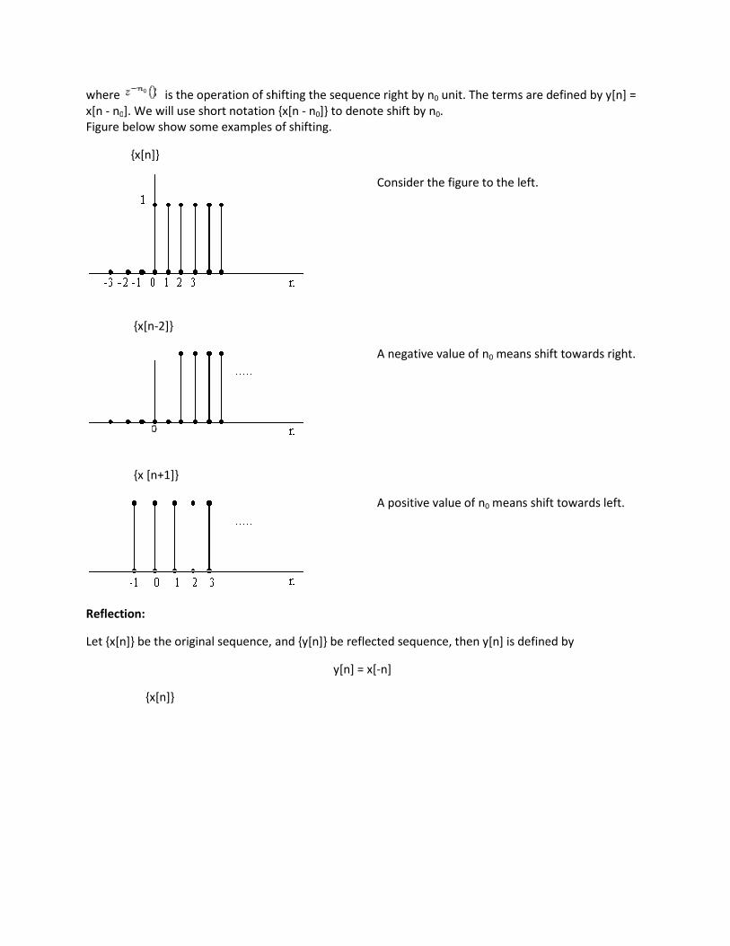
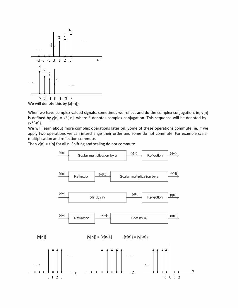


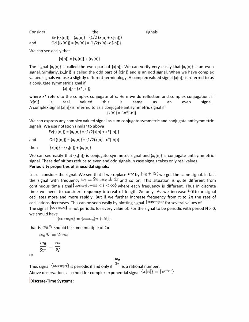


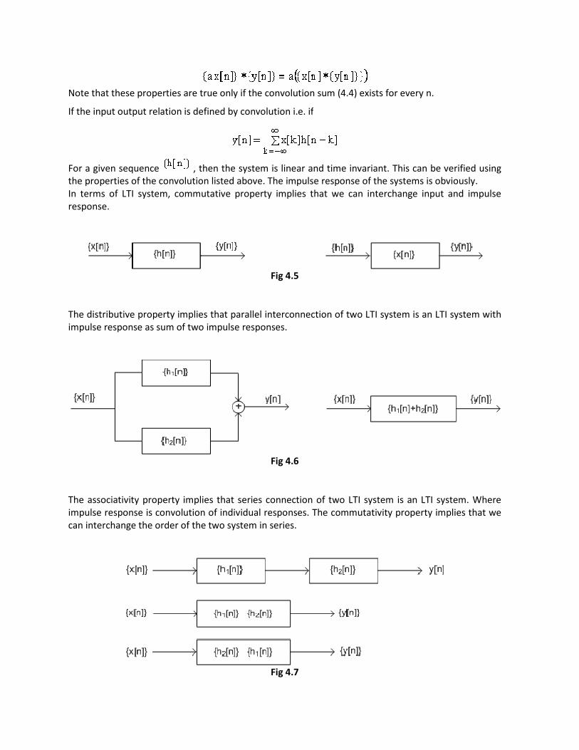
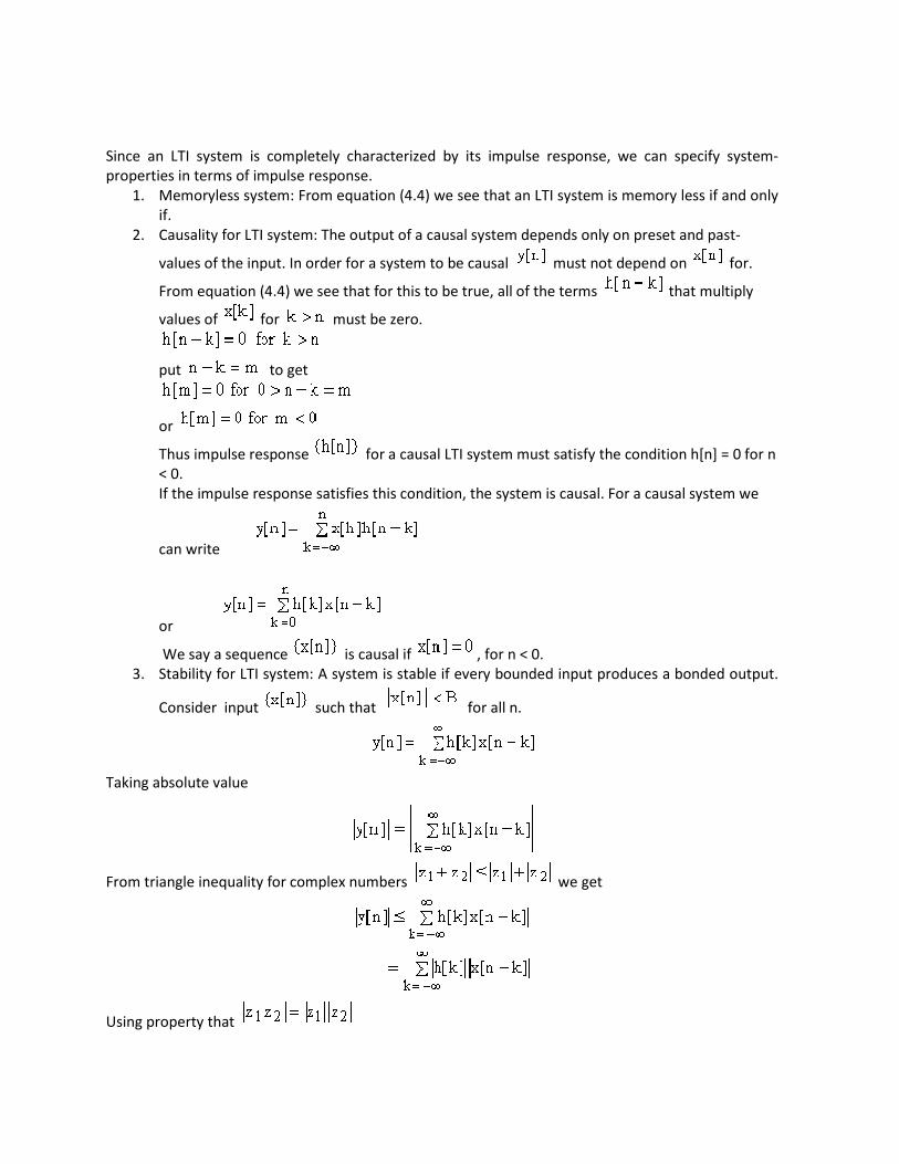
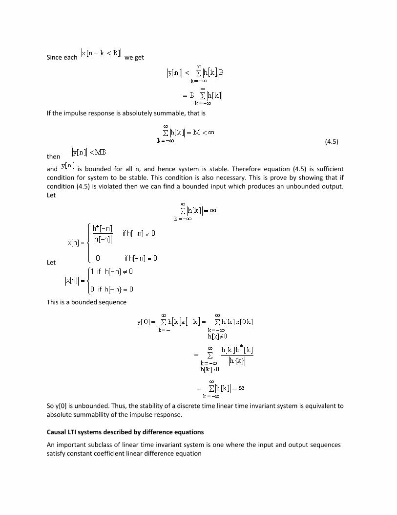


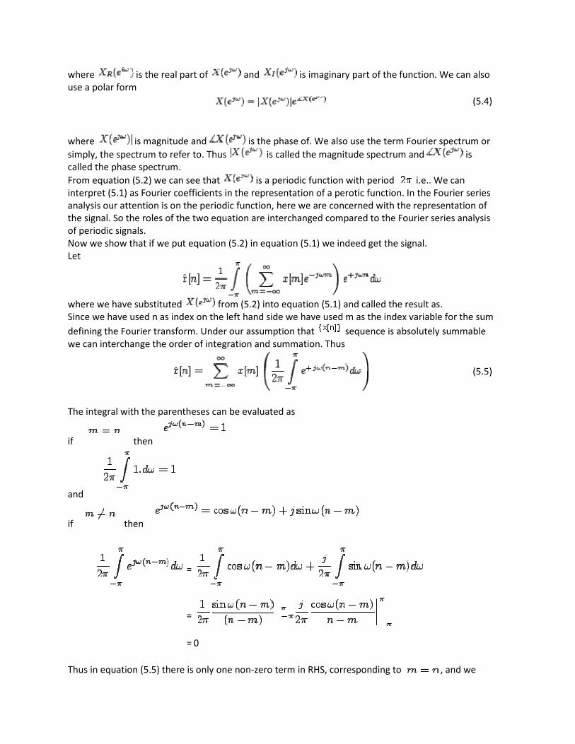


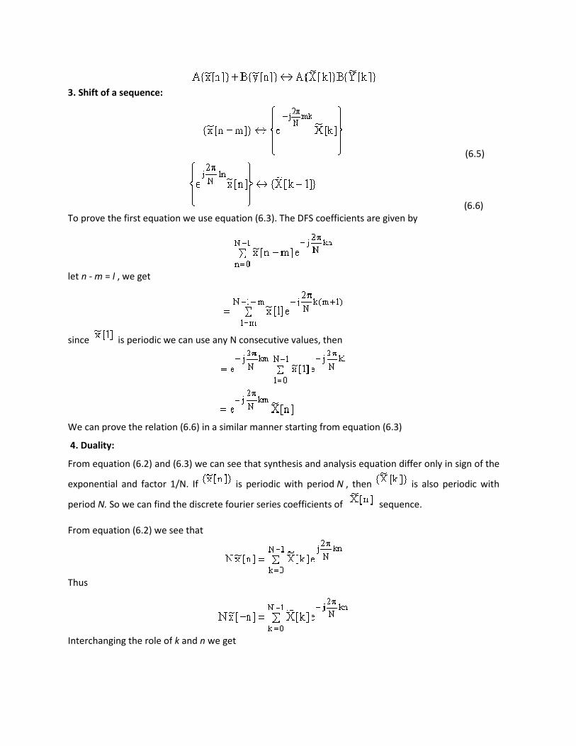

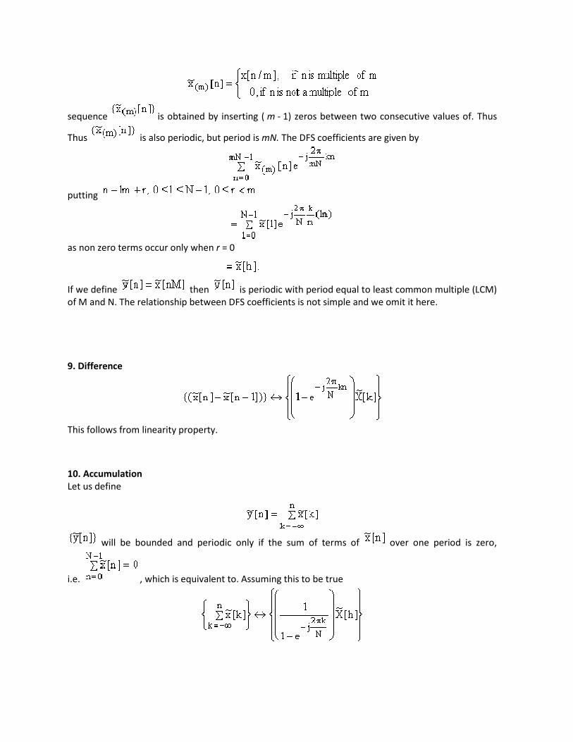

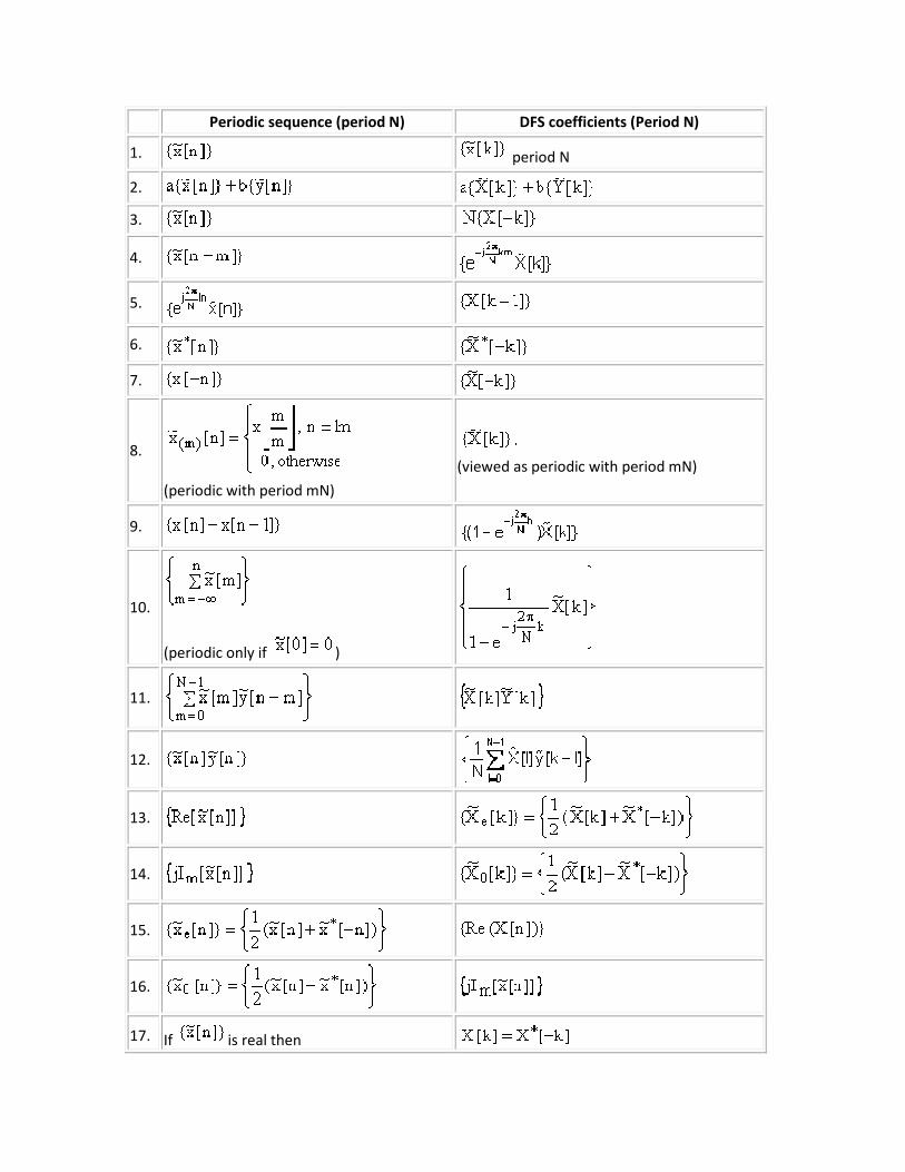


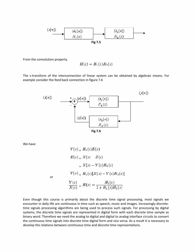


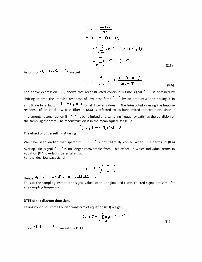


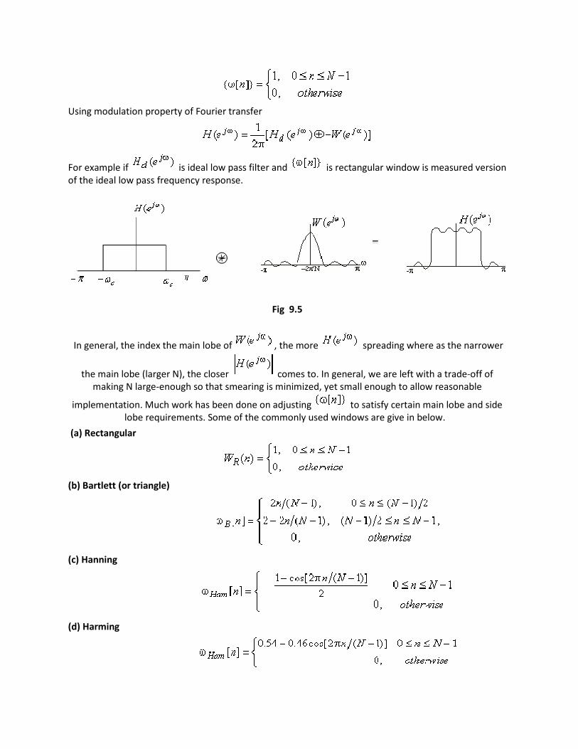


![Discrete Time Signal Processing · 2016. 6. 22. · When t denotes the time, we also refer to such a signal as a continuous-time signal. - Discrete signal: n ∈Z→x[n] ∈R or C](https://static.documents.pub/doc/80x56/612e24e81ecc51586942a09a/discrete-time-signal-processing-2016-6-22-when-t-denotes-the-time-we-also.jpg)


