Digital Signal Processing Markus Kuhn Computer Laboratory http://www.cl.cam.ac.uk/Teaching/2003/DigSigProc/ Easter 2004 – Part II Textbooks → R.G. Lyons: Understanding digital signal processing. Prentice- Hall, 2004. ( 45) → A.V. Oppenheim, R.W. Schafer: Discrete-time signal process- ing. 2nd ed., Prentice-Hall, 1999. ( 47) → J. Stein: Digital signal processing – a computer science per- spective. Wiley, 2000. ( 74) → S.W. Smith: Digital signal processing – a practical guide for engineers and scientists. Newness, 2003. ( 40) → K. Steiglitz: A digital signal processing primer – with appli- cations to digital audio and computer music. Addison-Wesley, 1996. ( 40) → Sanjit K. Mitra: Digital signal processing – a computer-based approach. McGraw-Hill, 2002. ( 38) 2
Transcript
Digital Signal Processing
Markus Kuhn
Computer Laboratory
http://www.cl.cam.ac.uk/Teaching/2003/DigSigProc/
Easter 2004 – Part II
Textbooks→ R.G. Lyons: Understanding digital signal processing. Prentice-
Hall, 2004. (£45)
→ A.V. Oppenheim, R.W. Schafer: Discrete-time signal process-
ing. 2nd ed., Prentice-Hall, 1999. (£47)
→ J. Stein: Digital signal processing – a computer science per-
spective. Wiley, 2000. (£74)
→ S.W. Smith: Digital signal processing – a practical guide for
engineers and scientists. Newness, 2003. (£40)
→ K. Steiglitz: A digital signal processing primer – with appli-
cations to digital audio and computer music. Addison-Wesley,1996. (£40)
→ Sanjit K. Mitra: Digital signal processing – a computer-based
approach. McGraw-Hill, 2002. (£38)
2
Digital signal processing
Concerned with algorithms to interpret, transform, and model wave-forms and the information they contain. Some typical applications:
→ geophysicsseismology, oil exploration
→ astronomyspeckle interferometry, VLBI
→ experimental physicssensor-data evaluation
→ communication systemsmodulation/demodulation, channelequalization, echo cancellation
where xn denotes the n-th number in the sequence (n ∈ Z). A discretesequence maps integer numbers onto real (or complex) numbers.The notation is not well standardized. Some authors write x[n] instead of xn, others x(n).
Where a discrete sequence {xn} samples a continuous function x(t) as
xn = x(ts · n) = x(n/fs),
we call ts the sampling period and fs = 1/ts the sampling frequency.
A discrete system T receives as input a sequence {xn} and transformsit into an output sequence {yn} = T{xn}:
A square-summable sequence is also called an energy signal, and
∞∑
n=−∞
|xn|2
its energy. This terminology reflects that if U is a voltage supplied to a load resistorR, then P = UI = U2/R is the power consumed.
So even where we drop physical units (e.g., volts) for simplicity in sequence calcu-lations, it is still customary to refer to the squared values of a sequence as power
and to its sum or integral over time as energy.5
A non-square-summable sequence is a power signal if its average power
limk→∞
1
1 + 2k
k∑
n=−k
|xn|2
exists.
Special sequences
Unit-step sequence:
un =
{
0, n < 01, n ≥ 0
Impulse sequence:
δn =
{
1, n = 00, n 6= 0
= un − un−1
6
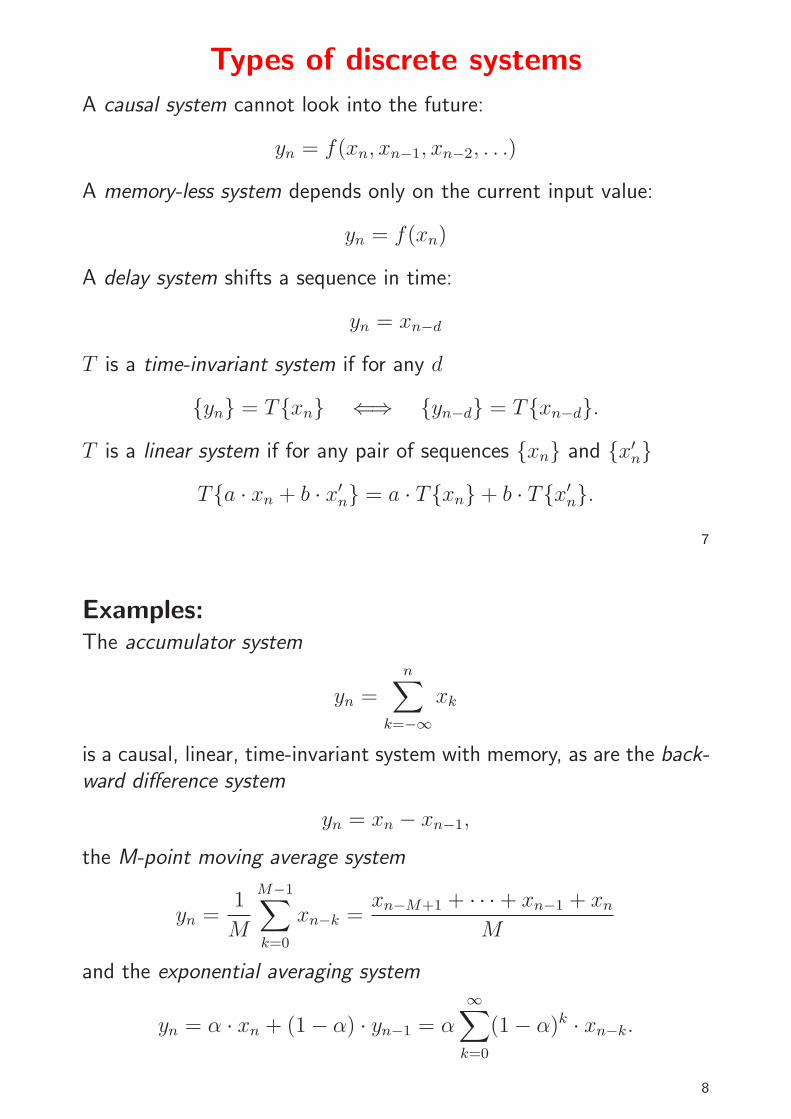
Types of discrete systems
A causal system cannot look into the future:
yn = f(xn, xn−1, xn−2, . . .)
A memory-less system depends only on the current input value:
yn = f(xn)
A delay system shifts a sequence in time:
yn = xn−d
T is a time-invariant system if for any d
{yn} = T{xn} ⇐⇒ {yn−d} = T{xn−d}.
T is a linear system if for any pair of sequences {xn} and {x′n}
T{a · xn + b · x′n} = a · T{xn} + b · T{x′
n}.
7
Examples:The accumulator system
yn =n∑
k=−∞xk
is a causal, linear, time-invariant system with memory, as are the back-
ward difference system
yn = xn − xn−1,
the M-point moving average system
yn =1
M
M−1∑
k=0
xn−k =xn−M+1 + · · · + xn−1 + xn
M
and the exponential averaging system
yn = α · xn + (1 − α) · yn−1 = α
∞∑
k=0
(1 − α)k · xn−k.
8
Examples for time-invariant non-linear memory-less systems are
yn = x2n, yn = log2 xn, yn = max{min{⌊256xn⌋, 255}, 0},
examples for linear but not time-invariant systems are
yn =
{
xn, n ≥ 00, n < 0
= xn · un
yn = x⌊n/4⌋
yn = xn · ℜ(eωjn)
and examples for linear time-invariant non-causal system are
yn =1
2(xn−1 + xn+1)
yn =9∑
k=−9
xn+k ·sin(πkω)
πkω· [0.5 + 0.5 · cos(πk/10)]
9
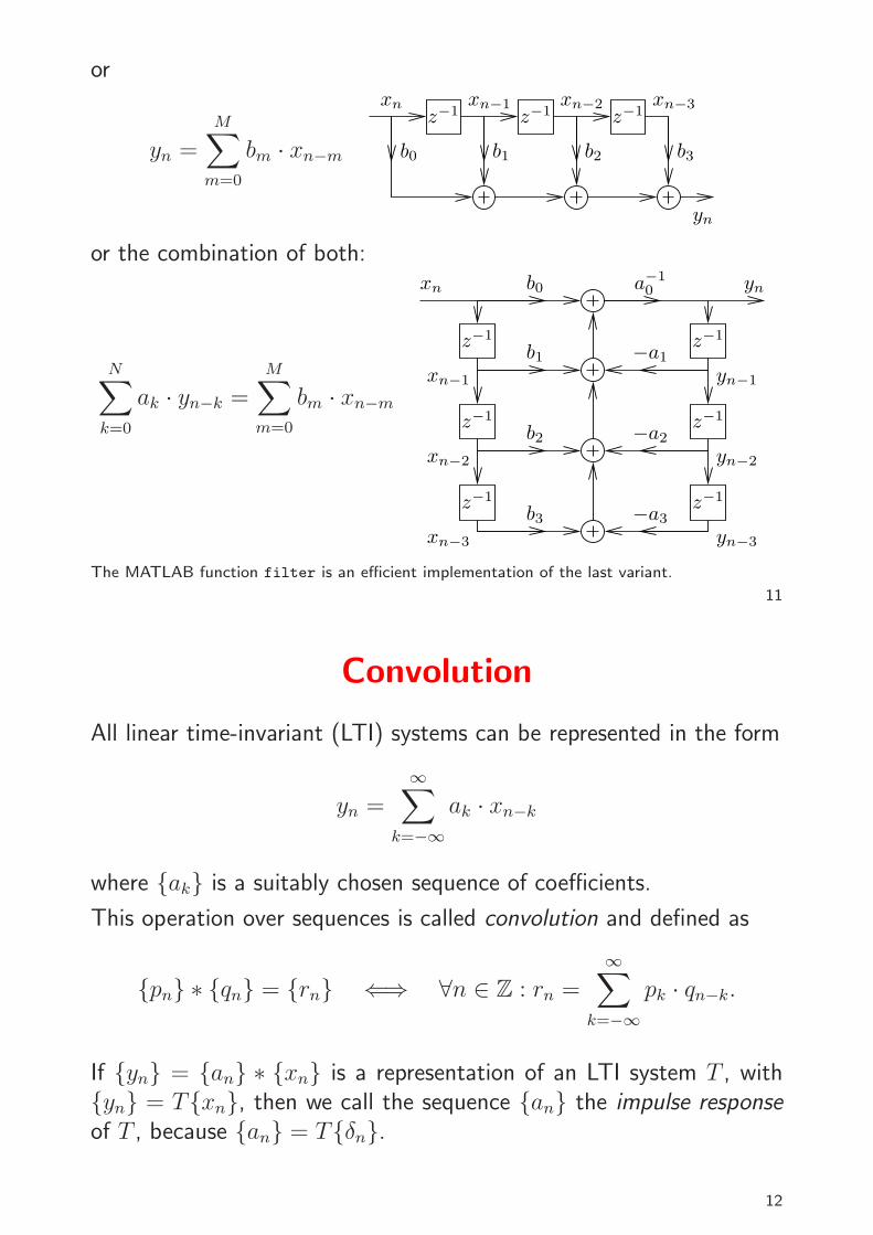
Constant-coefficient difference equationsOf particular practical interest are causal linear time-invariant systemsof the form
The MATLAB function filter is an efficient implementation of the last variant.
11
Convolution
All linear time-invariant (LTI) systems can be represented in the form
yn =∞∑
k=−∞ak · xn−k
where {ak} is a suitably chosen sequence of coefficients.
This operation over sequences is called convolution and defined as
{pn} ∗ {qn} = {rn} ⇐⇒ ∀n ∈ Z : rn =∞∑
k=−∞pk · qn−k.
If {yn} = {an} ∗ {xn} is a representation of an LTI system T , with{yn} = T{xn}, then we call the sequence {an} the impulse response
of T , because {an} = T{δn}.
12
Convolution examples
A B C D
E F A∗ B A∗ C
C∗ A A∗ E D∗ E A∗ F
13
Properties of convolutionFor arbitrary sequences {pn}, {qn}, {rn} and scalars a, b:
→ Convolution is associative
({pn} ∗ {qn}) ∗ {rn} = {pn} ∗ ({qn} ∗ {rn})
→ Convolution is commutative
{pn} ∗ {qn} = {qn} ∗ {pn}
→ Convolution is linear
{pn} ∗ {a · qn + b · rn} = a · ({pn} ∗ {qn}) + b · ({pn} ∗ {rn})
→ The impulse sequence (slide 6) is neutral under convolution
{pn} ∗ {δn} = {δn} ∗ {pn} = {pn}
→ Sequence shifting is equivalent to convolving with a shiftedimpulse
{pn−d} = {pn} ∗ {δn−d}14
Can all LTI systems be represented by convolution?Any sequence {xn} can be decomposed into a weighted sum of shiftedimpulse sequences:
{xn} =∞∑
k=−∞xk · {δn−k}
Let’s see what happens if we apply a linear(∗) time-invariant(∗∗) systemT to such a decomposed sequence:
T{xn} = T
( ∞∑
k=−∞xk · {δn−k}
)
(∗)=
∞∑
k=−∞xk · T{δn−k}
(∗∗)=
∞∑
k=−∞xk · {δn−k} ∗ T{δn} =
( ∞∑
k=−∞xk · {δn−k}
)
∗ T{δn}
= {xn} ∗ T{δn} q.e.d.
⇒ The impulse response T{δn} fully characterizes an LTI system.15
Exercise 1 A finite-length sequence is non-zero only at a finite number ofpositions. If m and n are the first and last non-zero positions, respectively,then we call n−m+1 the length of that sequence. What maximum lengthcan the result of convolving two sequences of length k and l have?
Exercise 2 The length-3 sequence a0 = −3, a1 = 2, a2 = 1 is convolvedwith a second sequence {bn} of length 5.
(a) Write down this linear operation as a matrix multiplication involving amatrix A, a vector ~b ∈ R
5, and a result vector ~c.
(b) Use MATLAB to multiply your matrix by the vector ~b = (1, 0, 0, 2, 2)and compare the result with that of using the conv function.
(c) Use the MATLAB facilities for solving systems of linear equations toundo the above convolution step.
Exercise 3 (a) Find a pair of sequences {an} and {bn}, where eithercontains at least three different values and where the convolution {an}∗{bn}results in an all-zero sequence.
(b) Does every LTI system T have an inverse LTI system T−1 such that{xn} = T−1T{xn} for all sequences {xn}? Why?
16
Direct form I and II implementations
z−1
z−1
z−1 z−1
z−1
z−1
b0
b1
b2
b3
a−10
−a1
−a2
−a3
xn−1
xn−2
xn−3
xn
yn−3
yn−2
yn−1
yn
=
z−1
z−1
z−1
a−10
−a1
−a2
−a3
xn
b3
b0
b1
b2
yn
The block diagram representation of the constant-coefficient differenceequation on slide 11 is called the direct form I implementation. Thenumber of delay elements can be halved by using the commutativityof convolution to swap the two feedback loops, leading to the direct
form II implementation of the same LTI system.17
Why are sine waves useful?
Adding together two sine waves of equal frequency, but arbitrary am-plitude and phase, results in another sine wave of the same frequency:
Convolution of a discrete sequence {xn} with another sequence {yn}is nothing but adding together scaled and delayed copies of {xn},according to a decomposition of {yn} into a sum of impulses. If {xn}was a sampled sine wave of frequency f , so will {xn} ∗ {yn} be.
=⇒ Sine-wave sequences form a family of discrete sequences that isclosed under convolution with arbitrary sequences.
Sine waves are orthogonal to each other
∫ ∞
−∞sin(ω1t + ϕ1) · sin(ω2t + ϕ2) dt = 0
⇐⇒ ω1 6= ω2 ∨ ϕ1 − ϕ2 = (2k + 1)π (k ∈ Z)
and therefore can be used to form an orthogonal function basis for atransform.
19
Complex phasorsAmplitude and phase are two distinct characteristics of a sine functionthat are inconvenient to keep separate notationally.
Complex functions (and discrete sequences) of the form
A · e jωt+ϕ = A · [cos(ωt + ϕ) + j · sin(ωt + ϕ)]
(where j2 = −1) are able to represent both amplitude and phase inone single algebraic object.
Thanks to complex multiplication, we can also incorporate in one singlefactor both a multiplicative change of amplitude and an additive changeof phase of such a function. This makes discrete sequences of the form
xn = e jωn
eigensequences with respect to an LTI system T , because for each ω,there is a complex number (eigenvalue) H(ω) such that
T{xn} = H(ω) · {xn}20
Recall: Fourier transformThe Fourier integral transform and its inverse are defined as
F{g(t)}(ω) = G(ω) = α
∫ ∞
−∞g(t) · e∓ jωt dt
F−1{G(ω)}(t) = g(t) = β
∫ ∞
−∞G(ω) · e± jωt dω
where α and β are constants chosen such that αβ = 1/(2π).Many equivalent forms of the Fourier transform are used in the literature, and there is no strongconsensus of whether the forward transform uses e− jωt and the backwards transform e jωt, orvice versa. Some authors set α = 1 and β = 1/(2π), to keep the convolution theorem free of aconstant prefactor, others use α = β = 1/
√2π, in the interest of symmetry.
The substitution ω = 2πf leads to a form without prefactors:
F{h(t)}(f) = H(f) =
∫ ∞
−∞h(t) · e∓2π jft dt
F−1{H(f)}(t) = h(t) =
∫ ∞
−∞H(f)· e±2π jft df
21
Another notation is in the continuous case
F{h(t)}(ω) = H(e jω) =
∫ ∞
−∞h(t) · e− jωt dt
F−1{H(e jω)}(t) = h(t) =1
2π
∫ ∞
−∞H(e jω) · e jωt dω
and in the discrete-sequence case
F{hn}(ω) = H(e jω) =∞∑
n=−∞hn · e− jωn
F−1{H(e jω)}(t) = hn =1
2π
∫
π
−π
H(e jω) · e jωn dω
which treats the Fourier transform as a special case of the z-transformto be introduced later.
22
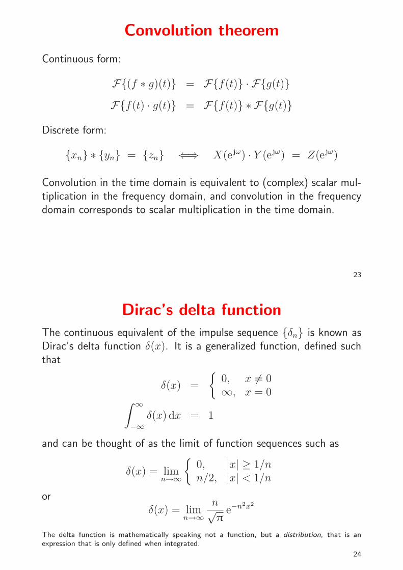
Convolution theorem
Continuous form:
F{(f ∗ g)(t)} = F{f(t)} · F{g(t)}
F{f(t) · g(t)} = F{f(t)} ∗ F{g(t)}
Discrete form:
{xn} ∗ {yn} = {zn} ⇐⇒ X(e jω) · Y (e jω) = Z(e jω)
Convolution in the time domain is equivalent to (complex) scalar mul-tiplication in the frequency domain, and convolution in the frequencydomain corresponds to scalar multiplication in the time domain.
23
Dirac’s delta function
The continuous equivalent of the impulse sequence {δn} is known asDirac’s delta function δ(x). It is a generalized function, defined suchthat
δ(x) =
{
0, x 6= 0∞, x = 0
∫ ∞
−∞δ(x) dx = 1
and can be thought of as the limit of function sequences such as
δ(x) = limn→∞
{
0, |x| ≥ 1/nn/2, |x| < 1/n
orδ(x) = lim
n→∞
n√π
e−n2x2
The delta function is mathematically speaking not a function, but a distribution, that is anexpression that is only defined when integrated.
24
Some properties of Dirac’s delta function:
∫ ∞
−∞f(x)δ(x − a) dx = f(a)
∫ ∞
−∞e±2π jftdf = δ(t)
1
2π
∫ ∞
−∞e± jωtdω = δ(t)
Fourier transform:
F{δ(t)}(ω) =
∫ ∞
−∞δ(t) · e− jωt dt = e0 = 1
F−1{1}(t) =1
2π
∫ ∞
−∞1 · e jωt dω = δ(t)
25
Sine and cosine in the frequency domain
cos(2πft) =1
2e2π jft +
1
2e−2π jft sin(2πft) =
1
2je2π jft − 1
2je−2π jft
−f f
−f
f
As any real-valued signal x(t) can be represented as a combinationof sine and cosine functions, the spectrum of any real-valued signalwill show the symmetry X(e jω) = [X(e− jω)]∗, where ∗ denotes thecomplex conjugate (i.e., negated imaginary part).
26
Sampling using a Dirac comb
The loss of information in the sampling process that converts a con-tinuous function x(t) into a discrete sequence {xn} defined by
xn = x(ts · n) = x(n/fs)
can be modelled through multiplying x(t) by a comb of Dirac impulses
s(t) =∞∑
n=−∞δ(t − ts · n)
to obtain the sampled function
x(t) = x(t) · s(t)
The function x(t) now contains exactly the same information as thediscrete sequence {xn}, but is still in a form that can be analysed usingthe Fourier transform on continuous functions.
27
The Fourier transform of a Dirac comb
s(t) =∞∑
n=−∞δ(t − ts · n)
is another Dirac comb
S(f) = F{ ∞∑
n=−∞δ(t − tsn)
}
(f) =
∞∫
−∞
∞∑
n=−∞δ(t − tsn) e2π jftdt =
1
ts
∞∑
n=−∞δ
(
f − n
ts
)
.
ts
s(t) S(f)
fs−2ts −ts 2ts −2fs −fs 2fs0 0 ft
28
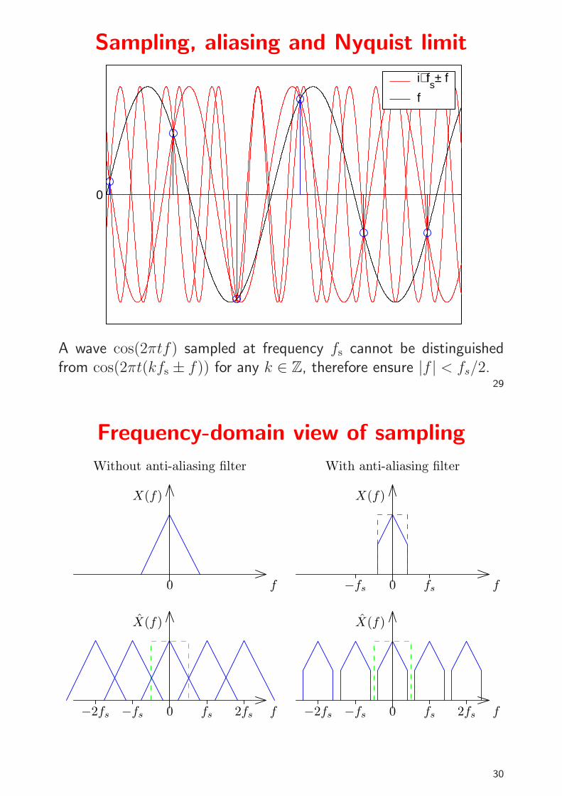
Sampling, aliasing and Nyquist limit
0
i⋅ fs± f
f
A wave cos(2πtf) sampled at frequency fs cannot be distinguishedfrom cos(2πt(kfs ± f)) for any k ∈ Z, therefore ensure |f | < fs/2.
29
Frequency-domain view of sampling
ffs−2fs −fs 0 2fs ffs−2fs −fs 0 2fs
f−fs 0f0 fs
Without anti-aliasing filter With anti-aliasing filter
X(f)
X(f)
X(f)
X(f)
30
Exercise 4� Generate a one second long Gaussian noise sequence {rn} (usingMATLAB function randn) with a sampling rate of 300 Hz.� Use the fir1(50, 45/150) function to design a finite impulse re-sponse low-pass filter with a cut-off frequency of 45 Hz. Use thefiltfilt function in order to apply that filter to the generated noisesignal, resulting in the filtered noise signal {xn}.� Then sample {xn} at 100 Hz by setting all but every third samplevalue to zero, resulting in sequence {yn}.� Generate another lowpass filter with a cut-off frequency of 50 Hz andapply it to {yn}, in order to interpolate the reconstructed filterednoise signal {zn}. Multiply the result by three, to compensate theenergy lost during sampling.� Plot {xn}, {yn}, and {zn}. Finally compare {xn} and {zn}.
Why should the first filter have a lower cut-off frequency than the second?
31
This page is intentionally left blank.
32
Reconstruction of a continuousband-limited waveform
The ideal anti-aliasing filter for eliminating any frequency content abovefs/2 before sampling with a frequency of fs has the Fourier transform
H(f) =
{
1 if −fs
2< f ≤ fs
2
0 otherwise.
This leads, after an inverse Fourier transform, to the impulse response
h(t) =sin πtfs
πtfs
.
The original band-limited signal can be reconstructed by convolvingthis with the sampled signal x(t), which eliminates the periodicity ofthe frequency domain introduced by the sampling process:
x(t) = h(t) ∗ x(t)
Note that sampling h(t) gives the impulse function: h(t) · s(t) = δ(t).33
−3 −2.5 −2 −1.5 −1 −0.5 0 0.5 1 1.5 2 2.5 3
−0.2
0
0.2
0.4
0.6
0.8
1
Impulse response of rectangular filter with cut−off frequency fs/2
t⋅ fs
34
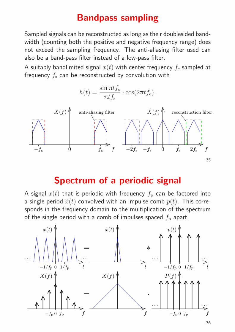
Bandpass sampling
Sampled signals can be reconstructed as long as their doublesided band-width (counting both the positive and negative frequency range) doesnot exceed the sampling frequency. The anti-aliasing filter used canalso be a band-pass filter instead of a low-pass filter.
A suitably bandlimited signal x(t) with center frequency fc sampled atfrequency fs can be reconstructed by convolution with
A signal x(t) that is periodic with frequency fp can be factored intoa single period x(t) convolved with an impulse comb p(t). This corre-sponds in the frequency domain to the multiplication of the spectrumof the single period with a comb of impulses spaced fp apart.
=
x(t)
t t t
= ∗
·
X(f)
f f f
p(t)x(t)
X(f) P (f)
. . . . . . . . . . . .
. . .. . .
−1/fp 1/fp0 −1/fp 1/fp0
0 fp−fp 0 fp−fp
36
Continuous versus discreteFourier transform� Sampling a continuous signal makes its spectrum periodic� A periodic signal has a sampled spectrum
=⇒ By taking n consecutive samples of a signal sampled with fs andrepeating these periodically, we obtain a signal with period n/fs, thespectrum of which is sampled at frequency intervals fs/n and repeatsitself with a period fs. Now both the signal and its spectrum are finitevectors of equal length.
X(f)
f
x(t)
t
. . .. . . . . . . . .
f−1sf−1
s 0−n/fs n/fs 0 fsfs/n−fs/n−fs
37
Properties of the Fourier transform
Ifx(t) ◦−• X(f) and y(t) ◦−• Y (f)
are pairs of functions that are mapped onto each other by the Fouriertransform, then so are the following pairs.
Linearity:ax(t) + by(t) ◦−• aX(f) + bY (f)
Time scaling:
x(at) ◦−• 1
|a| X
(
f
a
)
Frequency scaling:
1
|a| x
(
t
a
)
◦−• X(af)
38
Time shifting:
x(t − ∆t) ◦−• X(f) · e−2π jf∆t
Frequency shifting:
x(t) · e2π j∆ft ◦−• X(f − ∆f)
Parseval’s theorem (total power):
∫ ∞
−∞|x(t)|2dt =
∫ ∞
−∞|X(f)|2df
39
Fourier transform symmetries
We call a function x(t)
odd: x(−t) = −x(t)
even: x(−t) = x(t)
and ·∗ is the complex conjugate, such that (a + jb)∗ = (a − jb).
Then
x(t) is real ⇔ X(−f) = [X(f)]∗
x(t) is imaginary ⇔ X(−f) = −[X(f)]∗
x(t) is even ⇔ X(f) is evenx(t) is odd ⇔ X(f) is oddx(t) is real and even ⇔ X(f) is real and evenx(t) is real and odd ⇔ X(f) is imaginary and oddx(t) is imaginary and even ⇔ X(f) is imaginary and evenx(t) is imaginary and odd ⇔ X(f) is real and odd
40
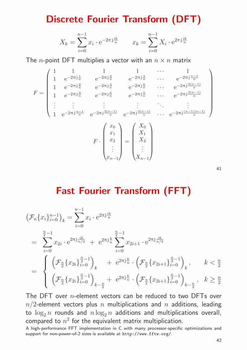
Discrete Fourier Transform (DFT)
Xk =n−1∑
i=0
xi · e−2π j ikn xk =
n−1∑
i=0
Xi · e2π j ikn
The n-point DFT multiplies a vector with an n × n matrix
F =
1 1 1 1 · · · 1
1 e−2π j 1n e−2π j 2
n e−2π j 3n · · · e−2π j
n−1n
1 e−2π j 2n e−2π j 4
n e−2π j 6n · · · e−2π j
2(n−1)n
1 e−2π j 3n e−2π j 6
n e−2π j 9n · · · e−2π j
3(n−1)n
......
......
. . ....
1 e−2π jn−1
n e−2π j2(n−1)
n e−2π j3(n−1)
n · · · e−2π j(n−1)(n−1)
n
F ·
x0
x1
x2
...xn−1
=
X0
X1
X2
...Xn−1
41
Fast Fourier Transform (FFT)
(
Fn{xi}n−1i=0
)
k=
n−1∑
i=0
xi · e2π j ikn
=
n2−1∑
i=0
x2i · e2π j ikn/2 + e2π j k
n
n2−1∑
i=0
x2i+1 · e2π j ikn/2
=
(
Fn2{x2i}
n2−1
i=0
)
k+ e2π j k
n ·(
Fn2{x2i+1}
n2−1
i=0
)
k, k < n
2
(
Fn2{x2i}
n2−1
i=0
)
k−n2
+ e2π j kn ·(
Fn2{x2i+1}
n2−1
i=0
)
k−n2
, k ≥ n2
The DFT over n-element vectors can be reduced to two DFTs overn/2-element vectors plus n multiplications and n additions, leadingto log2 n rounds and n log2 n additions and multiplications overall,compared to n2 for the equivalent matrix multiplication.A high-performance FFT implementation in C with many processor-specific optimizations andsupport for non-power-of-2 sizes is available at http://www.fftw.org/.
42
Efficient real-valued FFTThe symmetry properties of the Fourier transform applied to the discreteFourier transform {Xi}n−1
i=0 = Fn{xi}n−1i=0 have the form
∀i : xi = ℜ(xi) ⇐⇒ ∀i : Xn−i = X∗i
∀i : xi = j · ℑ(xi) ⇐⇒ ∀i : Xn−i = −X∗i
These two symmetries, combined with the linearity of the DFT, allows usto calculate two real-valued n-point DFTs
{X ′i}n−1
i=0 = Fn{x′i}n−1
i=0 {X ′′i }n−1
i=0 = Fn{x′′i }n−1
i=0
simultaneously in a single complex-valued n-point DFT, by composing itsinput as
xi = x′i + j · x′′
i
and decomposing its output as
X ′i =
1
2(Xi + X∗
n−i) X ′′i =
1
2(Xi − X∗
n−i)
To optimize the calculation of a single real-valued FFT, use this trick to calculate the two half-sizereal-value FFTs that occur in the first round.
43
Fast complex multiplication
The calculation of the product
(a + jb) · (c + jd) = (ac − bd) + j(ad + bc)
of two complex numbers costs four real-valued multiplications and twoadditions. On small processors, where multiplication is significantlyslower than addition, the calculation
provides the same result with just three multiplications, in exchangefor using three more (five) additions.
44
Polynomial representation of sequences
Example of polynomial multiplication:
(1 + 2v + 3v2) · (2 + 1v)
2 + 4v + 6v2
+ 1v + 2v2 + 3v3
= 2 + 5v + 8v2 + 3v3
Convolution:
conv([1 2 3], [2 1]) == [2 5 8 3]
We can represent sequences {xn} as polynomials:
X(v) =∞∑
n=−∞xnv
n
45
Convolution of sequences then becomes polynomial multiplication:
{hn} ∗ {xn} = {yn} =∞∑
k=−∞hk · xn−k
↓ ↓
H(v) · X(v) =
( ∞∑
n=−∞hnv
n
)
·( ∞∑
n=−∞xnv
n
)
=∞∑
n=−∞
∞∑
k=−∞hk · xn−k · vn
Note how the Fourier transform of a sequence can be accessed easilyfrom its polynomial form:
X(e− jω) =∞∑
n=−∞xne
− jωn
46
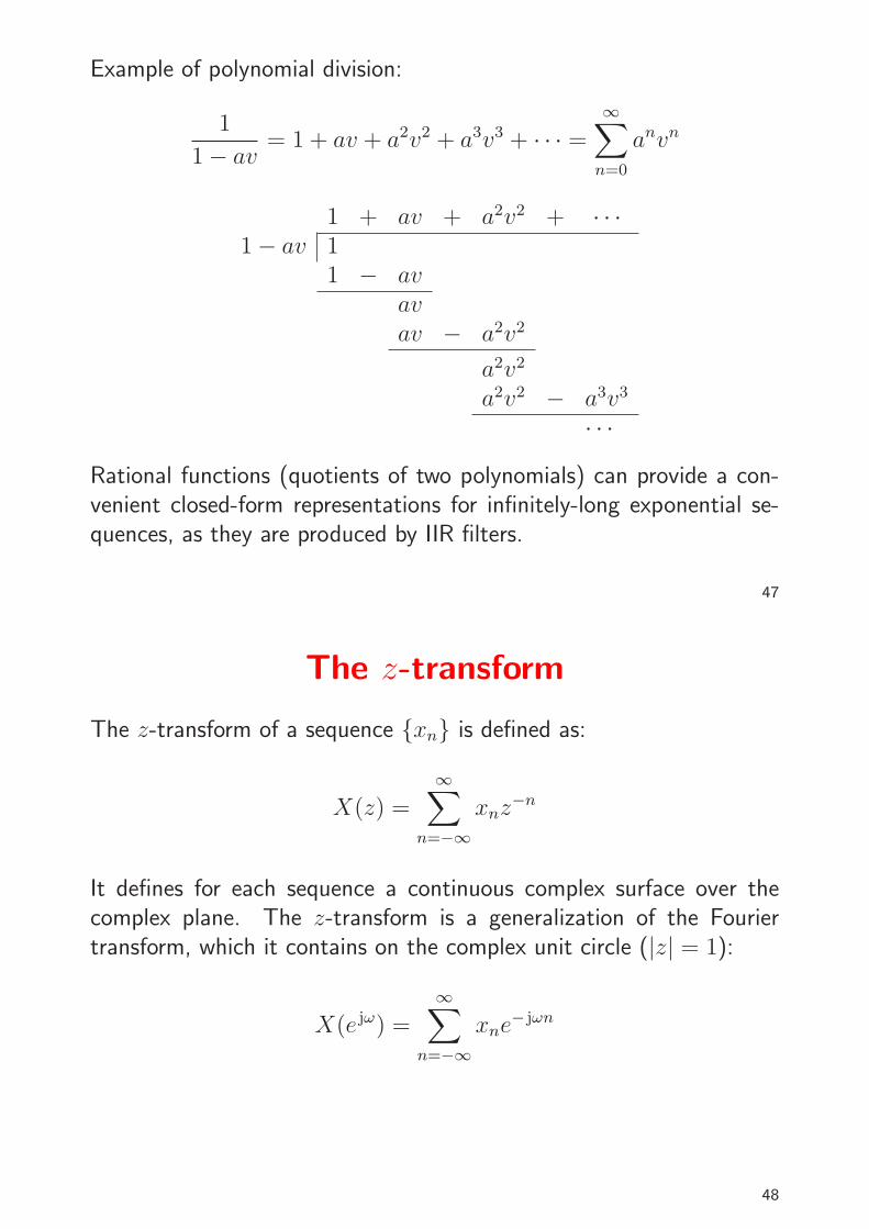
Example of polynomial division:
1
1 − av= 1 + av + a2v2 + a3v3 + · · · =
∞∑
n=0
anvn
1 + av + a2v2 + · · ·1 − av 1
1 − avavav − a2v2
a2v2
a2v2 − a3v3
· · ·
Rational functions (quotients of two polynomials) can provide a con-venient closed-form representations for infinitely-long exponential se-quences, as they are produced by IIR filters.
47
The z-transform
The z-transform of a sequence {xn} is defined as:
X(z) =∞∑
n=−∞xnz
−n
It defines for each sequence a continuous complex surface over thecomplex plane. The z-transform is a generalization of the Fouriertransform, which it contains on the complex unit circle (|z| = 1):
X(e jω) =∞∑
n=−∞xne
− jωn
48
The z-transform of the impulseresponse {hn} of the LTI definedby
N∑
k=0
ak · yn−k =M∑
m=0
bm · xn−m
with {yn} = {hn} ∗ {xn} is therational function
z−1
z−1
z−1 z−1
z−1
z−1
b0
b1
a−10
−a1
xn−1
xn
yn−1
yn
· · ·· · ·
· · ·· · ·
yn−k
−akbm
xn−m
H(z) =b0 + b1z
−1 + b2z−2 + · · · + bmz−m
a0 + a1z−1 + a2z−2 + · · · + akz−k
which can also be written as
H(z) =zn∑m
l=0 blzm−l
zm∑n
l=0 alzn−l
H(z) will have m zeros and n poles at non-zero location in the z plane,plus n − m zeros (if n > m) or m − n poles (if m > n) at z = 0.
49
This function can be converted into the form
H(z) =b0
a0
·
m∏
l=1
(1 − cl · z−1)
m∏
l=1
(1 − dl · z−1)
where the cl are the non-zero zeros and the dl the non-zero poles ofH(z). Except for a constant factor, H(z) is entirely characterized bythe position of these zeros and poles.
As with the Fourier transform, convolution in the time domain corre-sponds to complex multiplication in the z-domain:
{xn} ◦−• X(z), {yn} ◦−• Y (z) ⇒ {xn} ∗ {yn} ◦−• X(z) · Y (z)
Delaying a sequence by one corresponds in the z-domain to multipli-cation with z−1:
The design of a filter starts with specifying the desired parameters:
→ The passband is the frequency range where we want to approx-imate a gain of one.
→ The stopband is the frequency range where we want to approx-imate a gain of zero.
→ The order of a filter is the number of poles it uses in thez-domain, and equivalently the number of delay elements nec-essary to implement it.
→ Both passband and stopband will in practice not have gainsof exactly one and zero, respectively, but may show severaldeviations from these ideal values, and these ripples may havea specified maximum quotient between the highest and lowestgain.
60
→ There will in practice not be an abrupt change of gain betweenpassband and stopband, but a transition band where the fre-quency response will gradually change from its passband to itsstopband value.
The designer can then trade off conflicting goals such as a small tran-sition band, a low order, a low ripple amplitude, or even an absence ofripples.
Design techniques for making these tradeoffs for analog filters (involv-ing capacitors, resistors, coils) can also be used to design digital IIRfilters:
Butterworth filtersHave no ripples, gain falls monotonically across the pass and transitionband. Within the passband, the gain drops slowly down to 1 −
√
1/2(−3 dB). Outside the passband, it drops asymptotically by a factor 2N
per octave (N · 20 dB/decade).
61
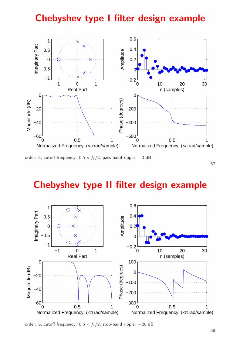
Chebyshev type I filtersDistribute the gain error uniformly throughout the passband (equirip-ples) and drop off monotonically outside.
Chebyshev type II filtersDistribute the gain error uniformly throughout the stopband (equirip-ples) and drop off monotonically in the passband.
Elliptic filters (Cauer filters)Distribute the gain error as equiripples both in the passband and stop-band. This type of filter is optimal in terms of the combination of thepassband-gain tolerance, stopband-gain tolerance, and transition-bandwidth that can be achieved at a given filter order.
All these filter design techniques are implemented in the MATLAB Signal Processing Toolbox inthe functions butter, cheby1, cheby2, and ellip, which output the coefficients an and bn of thedifference equation that describes the filter. These can be applied with filter to a sequence, orcan be visualized with zplane as poles/zeros in the z-domain, with impz as an impulse response,and with freqz as an amplitude and phase spectrum. The commands sptool and fdatool
provide interactive GUIs to design digital filters.
62
Discrete Fourier Transform visualized
·
x0
x1
x2
x3
x4
x5
x6
x7
=
X0
X1
X2
X3
X4
X5
X6
X7
The n-point DFT of a signal {xi} sampled at frequency fs contains inthe elements X0 to Xn/2 of the resulting frequency-domain vector thefrequency components 0, fs/n, 2fs/n, 3fs/n, . . . , fs/2, and containsin Xn−1 downto Xn/2 the corresponding negative frequencies. Notethat for a real-valued input vector, both X0 and Xn/2 will be real, too.Why is there no phase information recovered at fs/2?
63
Spectral estimation
0 10 20 30−1
−0.5
0
0.5
1
Sine wave 4×fs/32
0 10 20 300
5
10
15
Discrete Fourier Transform
0 10 20 30−1
−0.5
0
0.5
1
Sine wave 4.61×fs/32
0 10 20 300
5
10
15
Discrete Fourier Transform
64
We introduced the DFT as a special case of the continuous Fouriertransform, where the input is sampled and periodic.
If the input is sampled, but not periodic, the DFT can still be usedto calculate an approximation of the Fourier transform of the originalcontinuous signal. However, there are two effects to consider. Theyare particularly visible when analysing pure sine waves.
Sine waves whose frequency is a multiple of the base frequency (fs/n)of the DFT are identical to their periodic extension beyond the sizeof the DFT. They are therefore represented exactly by a single sharppeak in the DFT. All their energy falls into one single frequency “bin”in the DFT result.
Sine waves with other frequencies that do not match exactly one ofthe output frequency bins of the DFT are still represented by a peakat the output bin that represents the nearest integer multiple of theDFT’s base frequency. However, such a peak is distorted in two ways:
→ Its amplitude is lower (down to 63.7%)
→ Much signal energy has “leaked” to other frequencies.65
0 5 10 15 20 25 30 15
15.5
160
5
10
15
20
25
30
35
input freq.DFT index
The leakage of energy to other frequency bins not only blurs the estimated spec-trum. The peak amplitude also changes significantly as the frequency of a tonechanges from that associates with one output bin to the next, a phenomenonknown as scalloping. In the above graphic, an input sine wave gradually changesfrom the frequency of bin 15 to that of bin 16 (only positive frequencies shown).
66
Windowing
0 200 400−1
−0.5
0
0.5
1
Sine wave
0 200 4000
100
200
300Discrete Fourier Transform
0 200 400−1
−0.5
0
0.5
1
Sine wave multiplied with window function
0 200 4000
20
40
60
80Discrete Fourier Transform
67
The reason for the leakage and scalloping losses is easy to visualize with thehelp of the convolution theorem:
The operation of cutting a sequence with the size of the DFT input vectorout of a longer original signal (the one whose continuous Fourier spectrumwe try to estimate) is equivalent to multiplying this signal with a rectangularfunction. This destroys all information and continuity outside the “window”that is fed into the DFT.
Multiplication with a rectangular window of length T in the time domain isequivalent to convolution with sin(πfT )/(πfT ) in the frequency domain.
The subsequent interpretation of this window as a periodic sequence bythe DFT leads to sampling of this convolution result (sampling meaningmultiplication with a Dirac comb whose impulses are spaced fs/n apart).
Where the window length was an exact multiple of the original signal pe-riod, sampling of the sin(πfT )/(πfT ) leads to a single Dirac pulse, and thewindowing causes no distortion. In all other cases, the effects of the con-volution become visible in the frequency domain as leakage and scallopinglosses.
All these functions are 0 outside the interval [0,1].
69
0 0.5 1−60
−40
−20
0
20
Normalized Frequency (×π rad/sample)
Mag
nitu
de (
dB)
Rectangular window (64−point)
0 0.5 1−60
−40
−20
0
20
Normalized Frequency (×π rad/sample)
Mag
nitu
de (
dB)
Triangular window
0 0.5 1−60
−40
−20
0
20
Normalized Frequency (×π rad/sample)
Mag
nitu
de (
dB)
Hanning window
0 0.5 1−60
−40
−20
0
20
Normalized Frequency (×π rad/sample)
Mag
nitu
de (
dB)
Hamming window
70
Numerous alternatives to the rectangular window have been proposedthat reduce leakage and scalloping in spectral estimation. These arevectors multiplied element-wise with the input vector before applyingthe DFT to it. They all force the signal amplitude smoothly down tozero at the edge of the window, thereby avoiding the introduction ofsharp jumps in the signal when it is extended periodically by the DFT.
Three examples of such window vectors {wi}n−1i=0 are:
Triangular window (Bartlett window):
wi = 1 −∣
∣
∣
∣
1 − i
n/2
∣
∣
∣
∣
Hanning window (raised-cosine window, Hann window):
wi = 0.5 − 0.5 × cos
(
2πi
n − 1
)
Hamming window:
wi = 0.54 − 0.46 × cos
(
2πi
n − 1
)
71
Exercise 5 Explain the difference between the DFT, FFT, and FFTW.
Exercise 6 Push-button telephones use a combination of two sine tonesto signal, which button is currently being pressed:
1209 Hz 1336 Hz 1477 Hz 1633 Hz
697 Hz 1 2 3 A
770 Hz 4 5 6 B
852 Hz 7 8 9 C
941 Hz * 0 # D
(a) You receive a digital telephone signal with a sampling frequency of8 kHz. You cut a 256-sample window out of this sequence, multiply it with awindowing function and apply a 256-point DFT. What are the indices wherethe resulting vector (X0, X1, . . . , X255) will show the highest amplitude ifbutton 9 was pushed at the time of the recording?
(b) Use MATLAB to determine, which button sequence was typed in thetouch tones recorded in
Exercise 7 Draw the direct form II block diagrams of the causal infinite-impulse response filters described by the following z-transforms and writedown a formula describing their time-domain impulse responses:
(a) H(z) =1
1 − 12z−1
(b) H ′(z) =1 − 1
44 z−4
1 − 14z−1
(c) H ′′(z) =1
2+
1
4z−1 +
1
2z−2
Exercise 8 (a) Perform the polynomial division of the rational functiongiven in exercise 7 (a) until you have found the coefficient of z−5 in theresult.
(b) Perform the polynomial division of the rational function given in exercise7 (b) until you have found the coefficient of z−10 in the result.
(c) Has one of the filters in exercise 7 actually a finite impulse response,and if so, what is its z-transform?
73
Zero padding increases DFT resolutionThe two figures below show two spectra of the 16-element sequence
si = cos(2π · 3i/16) + cos(2π · 4i/16), i ∈ {0, . . . , 15}.The left plot shows the DFT of the windowed sequence
xi = si · wi, i ∈ {0, . . . , 15}and the right plot shows the DFT of the zero-padded windowed sequence
x′i =
{
si · wi, i ∈ {0, . . . , 15}0, i ∈ {16, . . . , 63}
where wi = 0.54 − 0.46 × cos (2πi/15) is the Hamming window.
0 5 10 150
2
4DFT without zero padding
0 20 40 600
2
4DFT with 48 zeros appended to window
74
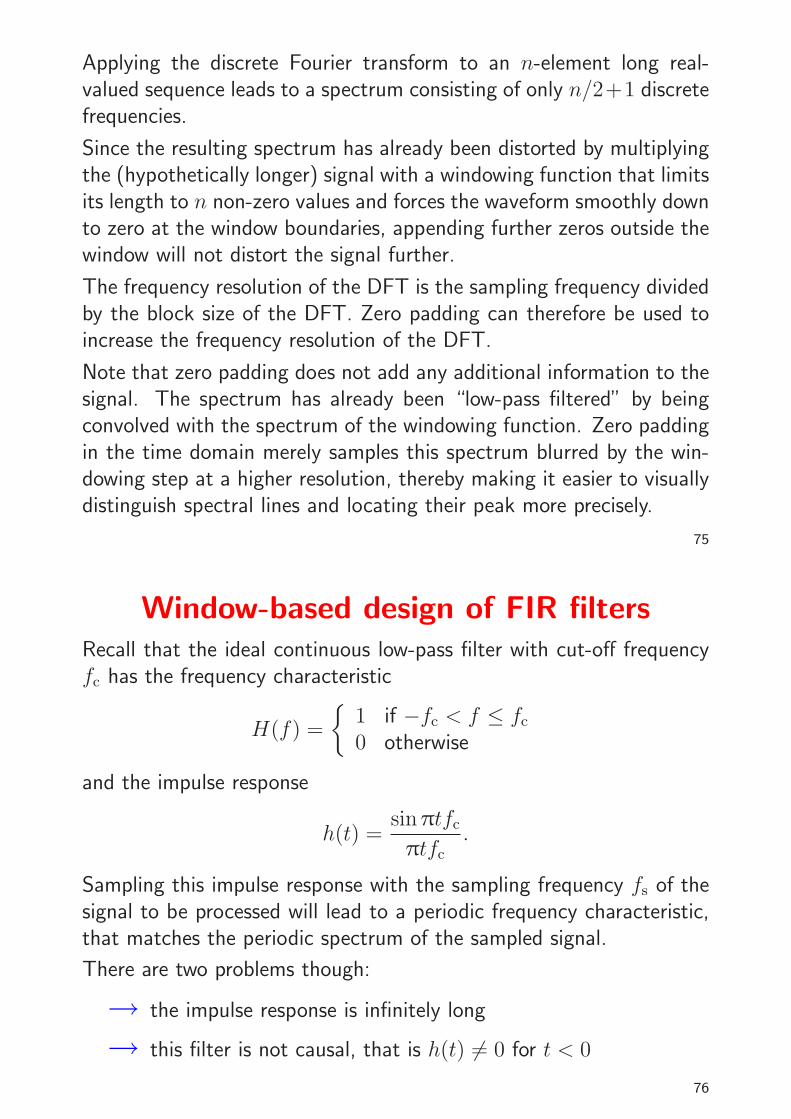
Applying the discrete Fourier transform to an n-element long real-valued sequence leads to a spectrum consisting of only n/2+1 discretefrequencies.
Since the resulting spectrum has already been distorted by multiplyingthe (hypothetically longer) signal with a windowing function that limitsits length to n non-zero values and forces the waveform smoothly downto zero at the window boundaries, appending further zeros outside thewindow will not distort the signal further.
The frequency resolution of the DFT is the sampling frequency dividedby the block size of the DFT. Zero padding can therefore be used toincrease the frequency resolution of the DFT.
Note that zero padding does not add any additional information to thesignal. The spectrum has already been “low-pass filtered” by beingconvolved with the spectrum of the windowing function. Zero paddingin the time domain merely samples this spectrum blurred by the win-dowing step at a higher resolution, thereby making it easier to visuallydistinguish spectral lines and locating their peak more precisely.
75
Window-based design of FIR filtersRecall that the ideal continuous low-pass filter with cut-off frequencyfc has the frequency characteristic
H(f) =
{
1 if −fc < f ≤ fc
0 otherwise
and the impulse response
h(t) =sin πtfc
πtfc
.
Sampling this impulse response with the sampling frequency fs of thesignal to be processed will lead to a periodic frequency characteristic,that matches the periodic spectrum of the sampled signal.
There are two problems though:
→ the impulse response is infinitely long
→ this filter is not causal, that is h(t) 6= 0 for t < 0
76
Solutions:
→ Make the impulse response finite by multiplying the sampledh(t) with a windowing function
→ Make the impulse response causal by adding a delay of half thewindow size
The impulse response of an n-th order low-pass filter is then chosen as
hi =sin[2π(i − n/2)fc/fs]
2π(i − n/2)fc/fs
· wi
where wi is a window function, such as the Hamming window
wi = 0.54 − 0.46 × cos (2πi/n)
with wi = 0 for i < 0 and i > n.Note that for fc = fs/4, we have hi = 0 for all even values of i. Therefore, this special caserequires only half the number of multiplications during the convolution. Such “half-band” FIRfilters are used, for example, as anti-aliasing filters wherever a sampling rate needs to be halved.
77
FIR lowpass filter design example
−1 0 1
−1
−0.5
0
0.5
1
30
Real Part
Imag
inar
y P
art
0 10 20 30−0.1
0
0.1
0.2
0.3
n (samples)
Am
plitu
de
0 0.5 1−60
−40
−20
0
Normalized Frequency (×π rad/sample)
Mag
nitu
de (
dB)
0 0.5 1−1500
−1000
−500
0
Normalized Frequency (×π rad/sample)
Pha
se (
degr
ees)
order: 30, cutoff frequency (−6 dB): 0.25 × fs/2
78
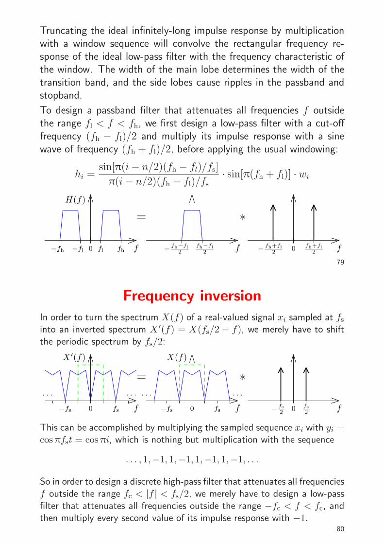
Truncating the ideal infinitely-long impulse response by multiplicationwith a window sequence will convolve the rectangular frequency re-sponse of the ideal low-pass filter with the frequency characteristic ofthe window. The width of the main lobe determines the width of thetransition band, and the side lobes cause ripples in the passband andstopband.
To design a passband filter that attenuates all frequencies f outsidethe range fl < f < fh, we first design a low-pass filter with a cut-offfrequency (fh − fl)/2 and multiply its impulse response with a sinewave of frequency (fh + fl)/2, before applying the usual windowing:
hi =sin[π(i − n/2)(fh − fl)/fs]
π(i − n/2)(fh − fl)/fs
· sin[π(fh + fl)] · wi
= ∗
0 0f f ffhfl
H(f)
fh+fl2
−fh −fl − fh−fl2
fh−fl2
− fh+fl2
79
Frequency inversion
In order to turn the spectrum X(f) of a real-valued signal xi sampled at fs
into an inverted spectrum X ′(f) = X(fs/2 − f), we merely have to shiftthe periodic spectrum by fs/2:
= ∗
0 0f f f
X(f)
−fs fs 0−fs fs
X ′(f)
fs2
− fs2
. . . . . .. . .. . .
This can be accomplished by multiplying the sampled sequence xi with yi =cos πfst = cos πi, which is nothing but multiplication with the sequence
. . . , 1,−1, 1,−1, 1,−1, 1,−1, . . .
So in order to design a discrete high-pass filter that attenuates all frequenciesf outside the range fc < |f | < fs/2, we merely have to design a low-passfilter that attenuates all frequencies outside the range −fc < f < fc, andthen multiply every second value of its impulse response with −1.
80
FFT-based convolutionCalculating the convolution of two finite sequences {xi}m−1
i=0 and {yi}n−1i=0
of lengths m and n via
zi =
min{m−1,i}∑
j=max{0,i−(n−1)}xj · yi−j, 0 ≤ i < m + n − 1
takes mn multiplications.
Can we apply the FFT and the convolution theorem to calculate theconvolution faster, in just O(m log m + n log n) multiplications?
{zi} = F−1 (F{xi} · F{yi})
There is obviously no problem if this condition is fulfilled:
{xi} and {yi} are periodic, with equal period lengths
In this case, the fact that the DFT interprets its input as a single periodof a periodic signal will do exactly what is needed, and the FFT andinverse FFT can be applied directly as above.
81
In the general case, measures have to be taked to prevent a wrap-over:
A B F−1[F(A)⋅F(B)]
A’ B’ F−1[F(A’)⋅F(B’)]
Both sequences are padded by appending zero values to a length ofat least m + n − 1, to ensure that the start and end of the resultingsequence to not overlap.
82
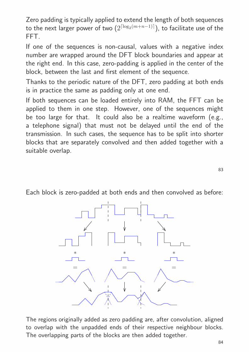
Zero padding is typically applied to extend the length of both sequencesto the next larger power of two (2⌈log2(m+n−1)⌉), to facilitate use of theFFT.
If one of the sequences is non-causal, values with a negative indexnumber are wrapped around the DFT block boundaries and appear atthe right end. In this case, zero-padding is applied in the center of theblock, between the last and first element of the sequence.
Thanks to the periodic nature of the DFT, zero padding at both endsis in practice the same as padding only at one end.
If both sequences can be loaded entirely into RAM, the FFT can beapplied to them in one step. However, one of the sequences mightbe too large for that. It could also be a realtime waveform (e.g.,a telephone signal) that must not be delayed until the end of thetransmission. In such cases, the sequence has to be split into shorterblocks that are separately convolved and then added together with asuitable overlap.
83
Each block is zero-padded at both ends and then convolved as before:
= = =
∗ ∗ ∗
The regions originally added as zero padding are, after convolution, alignedto overlap with the unpadded ends of their respective neighbour blocks.The overlapping parts of the blocks are then added together.
84
Random sequences and noiseA discrete random sequence {xn} is a sequence of numbers
. . . , x−2, x−1, x0, x1, x2, . . .
where each value xn is the outcome of a random variable xn in acorresponding sequence of random variables
. . . ,x−2,x−1,x0,x1,x2, . . .
Such a collection of random variables is called a random process. Eachindividual random variable xn is characterized by its probability distri-bution function
Pxn(a) = Prob(xn ≤ a)
and the entire random process is characterized completely by all jointprobability distribution functions
Pxn1,...,xnk
(a1, . . . , ak) = Prob(xn1≤ a1 ∧ . . . ∧ xnk
≤ ak)
for all possible sets {xn1, . . . ,xnk
}.85
Two random variables xn and xm are called independent if
Pxn,xm(a, b) = Pxn(a) · Pxm(b)
and a random process is called stationary if
Pxn1+l,...,xnk+l(a1, . . . , ak) = Pxn1
,...,xnk(a1, . . . , ak)
for all l, in other words, if the probability distributions are time invari-ant.
The derivative pxn(a) = P ′xn
(a) is called the probability density func-
tion, and helps us to define quantities such as
→ the expected value E(xn) =∫
apxn(a) da
→ the mean-square value (average power) E(|xn|2)→ the variance Var(xn) = E [|xn−E(xn)|2] = E(|xn|2)−|E(xn)|2
→ the correlation Cor(xn,xm) = E(xn · x∗m)
Remember that E(·) is linear, that is E(ax) = aE(x) and E(x + y) = E(x) + E(y). Also,Var(ax) = a2Var(x) and, if x and y are independent, Var(x + y) = Var(x) + Var(y).
86
A stationary random process {xn} can be characterized by its meanvalue
mx = E(xn),
its varianceσ2
x = E(|xn − mx|2) = γxx(0)
(σx is also called standard deviation), its autocorrelation sequence
A stationary pair of random processes {xn} and {yn} can, in addition,be characterized by its crosscorrelation sequence
φxy(k) = E(xn+k · y∗n)
and its crosscovariance sequence
γxy(k) = E [(xn+k − mx) · (yn − my)∗] = φxy(k) − mxm
∗y
87
Deterministic crosscorrelation sequenceFor deterministic sequences {xn} and {yn}, the crosscorrelation sequence
is
cxy(k) =∞∑
i=−∞xi+kyi.
After dividing through the overlapping length of the finite sequences involved, cxy(k) can beused to estimate from a finite sample of a stationary random sequence the underlying φxy(k).MATLAB’s xcorr function does that with option unbiased.
If {xn} is similar to {yn}, but lags l elements behind (xn ≈ yn−l), thencxy(l) will be a peak in the crosscorrelation sequence. It is therefore widelycalculated to locate shifted versions of a known sequence in another one.
The crosscorrelation is a close cousin of the convolution, with just the secondinput sequence mirrored:
{cxy(n)} = {xn} ∗ {y−n}It can therefore be calculated equally easily via the Fourier transform:
Cxy(f) = X(f) · Y ∗(f)
Swapping the input sequences mirrors the output sequence: cxy(k) = cyx(−k)
88
Equivalently, we define the autocorrelation sequence in the time-domainas
cxx(k) =∞∑
i=−∞xi+kxi.
which corresponds in the frequency domain to
Cxx(f) = X(f) · X∗(f) = |X(f)|2.
In other words, the Fourier transform Cxx(f) of the autocorrelationsequence {cxx(n)} of a sequence {xn} is identical to the squared am-plitudes of the Fourier transform or power spectrum of {xn}.This suggests, that the Fourier transform of the autocorrelation se-quence of a random process might be a suitable way for defining thepower spectrum of that random process.
89
Filtered random sequencesLet {xn} be a random sequence from a stationary random process.The output
yn =∞∑
k=−∞hk · xn−k =
∞∑
k=−∞hn−k · xk
of an LTI applied to it will then be another random sequence, charac-terized by
White noiseA random sequence {xn} is a white noise signal, if mx = 0 and
φxx(k) = σ2xδk.
The power spectrum of a white noise signal is flat:
Φxx(f) = σ2x.
Application example:
Where an LTI {yn} = {hn} ∗ {xn} can be observed to operate onwhite noise {xn} with φxx(k) = σ2
xδk, the crosscorrelation betweeninput and output will reveal the impulse response of the system:
φxy(n) = σ2x · hn.
91
Averaging and noise reduction
Often an original signal {xi} is only accessible with some added noise
{yi} = {xi} + {ni}
which turns a deterministic sequence into a random sequence. Thesignal-to-noise ratio (SNR) of the received signal {yi} is the square rootof the power ratio of these components: SNRy =
√
E(|xi|2)/E(|ni|2).As an SNR might also be given in terms of a power ratio, it is commonly expressed in decibels,to avoid any confusion between power and voltage ratios: 10 dB · log10 E(|xi|2)/E(|ni|2) =
20 dB · log10
p
E(|xi|2)/E(|ni|2).
The simplest noise reduction technique is averaging. If we know thatthe k signal values x1, . . . , xk are identical, and the noise average ismn = 0, then we can calculate an average value
y =1
k
k∑
i=1
yi
as an approximation for the true value x1 = · · · = xk.92
What noise level remains after averaging?The k identical signal values x1, . . . , xk are characterized by mx = xi
(i = 1, . . . , k) and σ2x = 0. The average signal power is E(|xi|2) = m2
x.
We assume that the k noise values n1, . . . , nk are statistically indepen-dent and are the output of a stationary process with mean mn = 0and variance σ2
n. The average noise power is E(|ni|2) = σ2n.
The averaging result y can be split up into a signal component x anda noise component n:
y =1
k
k∑
i=1
yi =1
k
k∑
i=1
xi +1
k
k∑
i=1
ni = x + n
The corresponding average power values are
E(|x|2) = E
∣
∣
∣
∣
∣
1
k
k∑
i=1
xi
∣
∣
∣
∣
∣
2
= E
∣
∣
∣
∣
∣
1
k
k∑
i=1
mx
∣
∣
∣
∣
∣
2
= m2x
93
and
E(|n|2) = Var(n) = Var
(
1
k
k∑
i=1
ni
)
=1
k2
k∑
i=1
Var(ni) =1
kσ2
n.
We can now compare the signal-to-noise ratio of the original noisysequence
SNRy =
√
E(|xi|2)E(|ni|2)
=mx
σn
with that of the averaging result
SNRy =
√
E(|x|2)E(|n|2) =
√k · mx
σn
.
Averaging k samples of identical signal values with added independentzero-mean noise values will increase the signal-to-noise ratio by thefactor
√k.
Remember that adding identical values x1 and x2 will double their value and therefore quadrupletheir power. On the other hand, adding independent zero-mean noise values n1 and n2 will – onaverage – only double their power (= variance).
94
Noise reduction filters
Added independent noise values with φnn(k) = σ2nδk have a flat spec-
trum Φnn(f) = σ2n, which is added in {yi} = {xi} + {ni} across the
spectrum of the noise-free signal {xi}.Knowledge of the power spectrum X(f) of the original signal can helpto design a filter that attenuates much of the noise in {yi}, withoutdegrading the wanted signal {xi} too much. If {xi} changes veryslowly, most of its energy will be at low frequencies, and noise can bereduced with a suitably chosen low-pass filter.
If there are no significant changes in {xi} during k consecutive samples,then convolution with a k samples wide rectangular window will notaffect the wanted signal.
We have already seen that this will reduce the noise amplitude by afactor
√k, or equivalently the noise power by a factor of k.
95
How does a general LTI filter
yi =∞∑
k=−∞hk · yi−k =
∞∑
k=−∞hk · (xi−k + ni−k) = xi + ni
affect the signal-to-noise ratio SNRy =√
E(|xi|2)/E(|ni|2)?With mx ≈ xi, we get
E(|xi|2) = E
∣
∣
∣
∣
∣
∞∑
k=−∞hkxi−k
∣
∣
∣
∣
∣
2
= m2x
∣
∣
∣
∣
∣
∞∑
k=−∞hk
∣
∣
∣
∣
∣
2
and
E(|ni|2) = Var(ni) =
Var
( ∞∑
k=−∞hkni−k
)
=∞∑
k=−∞h2
k · Var(ni−k) = σ2n
∞∑
k=−∞h2
k
⇒ SNRyi/SNRyi
=∣
∣
∑∞k=−∞ hk
∣
∣ /√
∑∞k=−∞ h2
k96
Exponential averagingA particularly easy to implement IIR low-pass filter, with only one delay element,is the exponential averaging filter
z−1
yi
α
1 − α
yi
yi−1
yi = (1 − α)yi + αyi−1 = (1 − α)∞∑
k=0
αkyi−k, (0 ≤ α < 1).
When applied as a noise filter on a sequence {yi} = {xi} + {ni} withσ2
x = 0, mn = 0, and mutually independent noise values {ni}, we get
σ2yi
= (1 − α)2
∞∑
k=0
α2kσ2yi−k
= σ2n(1 − α)2
∞∑
k=0
α2k =
σ2n(1 − α)2 · 1
1 − α2= σ2
n · 1 − α
1 + α
and therefore SNRyi/SNRyi
=mx
σyi
/mx
σn
=
√
1 + α
1 − α.
97
DFT averaging
The above diagrams show different type of spectral estimates of a sequencexi = sin(2πj × 8/64) + sin(2πj × 14.32/64) + ni with φnn(i) = 4δi.
Left is a single 64-element DFT of {xi} (with rectangular window). Theflat spectrum of white noise is only an expected value. In a single discreteFourier transform of such a sequence, the significant variance of the noisespectrum becomes visible. It almost drowns the two peaks from sine waves.
After cutting {xi} into 1000 windows of 64 elements each, calculating theirDFT, and plotting the average of their absolute values, the centre figureshows an approximation of the expected value of the amplitude spectrum,with a flat noise floor. Taking the absolute value before averaging is calledincoherent averaging, as the phase information is thrown away.
The rightmost figure was generated from the same set of 1000 windows,but this time the complex values of the DFTs were averaged before the
98
absolute value was taken. This is called coherent averaging and, becauseof the linearity of the DFT, identical to first averaging the 1000 windowsand then applying a single DFT and taking its absolute value. The windowsstart 64 samples apart. Only periodic waveforms with a period that divides64 are not averaged away. This periodic averaging step suppresses both thenoise and the second sine wave.
Periodic averaging
If a zero-mean signal {xi} has a periodic component with period p, theperiodic component can be isolated by periodic averaging :
xi = limk→∞
1
2k + 1
k∑
n=−k
xi+pn
Periodic averaging corresponds in the time domain to convolution with aDirac comb
∑
n δi−pn. In the frequency domain, this means multiplicationwith a Dirac comb that eliminates all frequencies but multiples of 1/p.
99
Exercise 9 A tumble dryer measures the air humidity xi in the drumtwice per second, but the control software uses only a smoothed valueyi =
∑15k=0 xi−k to decide when to stop the drying programme.
(a) Assuming that humidity fluctuations in a tumble dryer have compo-nents that are periodic with the rotational frequency of the drum, for whichrotational speeds would the above smoothing filter suppress these periodiccomponents particularly well?
(b) It is the year 2020, and a cartel of semiconductor manufacturers recentlymanaged to double the cost of memory every 18 months. Your job is toredesign products to eliminate unnecessary use of precious memory. Replacethe above data smoothing algorithm with one that requires the least amountof memory possible, but that reduces the random fluctuations caused in themeasurements by tumbling clothes by exactly the same factor. You nowcan assume that these fluctuations are not correlated between differentmeasurements xi.
(c) First predict the approximate shape of the frequency characteristic ofboth the old and the new smoothing filter, then use MATLAB to plot it.


![ECE-V-DIGITAL SIGNAL PROCESSING [10EC52] …vtusolution.in/.../digital-signal-processing-10ec52.pdfDigital vtusolution.in Signal Processing 10EC52 TEXT BOOK: 1. DIGITAL SIGNAL PROCESSING](https://static.documents.pub/doc/80x56/5afe42bb7f8b9a256b8ccd2e/ece-v-digital-signal-processing-10ec52-signal-processing-10ec52-text-book.jpg)


