Digital Transmission Fundamentals

Digital Representation of InformationWhy Digital Communications?

Signal Time Variations And BandwidthCharacterization of Communication Channels

Fundamental Limits in Digital TransmissionLine Coding

Modems and Digital ModulationProperties of Media and Digital Transmission Systems

Error Detection and Correction

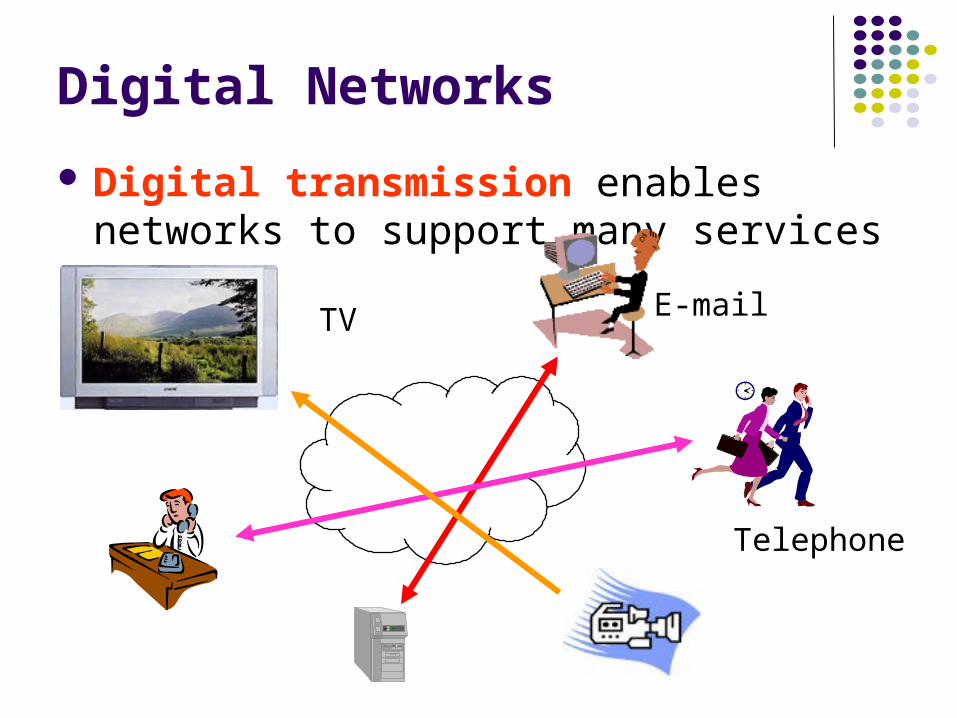
Digital Networks

Digital transmission enables networks to support many services

E-mail

Telephone

TV

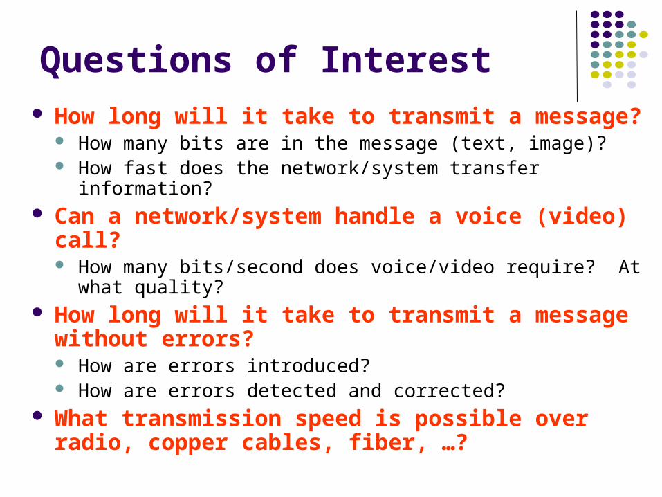
Questions of Interest How long will it take to transmit a message?

How many bits are in the message (text, image)? How fast does the network/system transfer information?

Can a network/system handle a voice (video) call? How many bits/second does voice/video require? At what

quality? How long will it take to transmit a message without

errors? How are errors introduced? How are errors detected and corrected?

What transmission speed is possible over radio, copper cables, fiber, …?

Digital Transmission Fundamentals

Digital Representation of Information

Bits, numbers, information

Bit: number with value 0 or 1 n bits: digital representation for 0, 1, … , 2n-1 Byte or Octet, n = 8 Computer word, n = 16, 32, or 64

n bits allows enumeration of 2n possibilities n-bit field in a header n-bit representation of a voice sample Message consisting of n bits

The number of bits required to represent a message is a measure of its information content More bits → More content

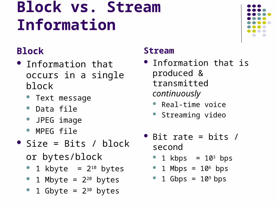
Block vs. Stream Information

Block Information that occurs

in a single block Text message Data file JPEG image MPEG file

Size = Bits / block

or bytes/block 1 kbyte = 210 bytes 1 Mbyte = 220 bytes 1 Gbyte = 230 bytes

Stream Information that is

produced & transmitted continuously Real-time voice Streaming video

Bit rate = bits / second 1 kbps = 103 bps 1 Mbps = 106 bps 1 Gbps = 109 bps

Transmission Delay

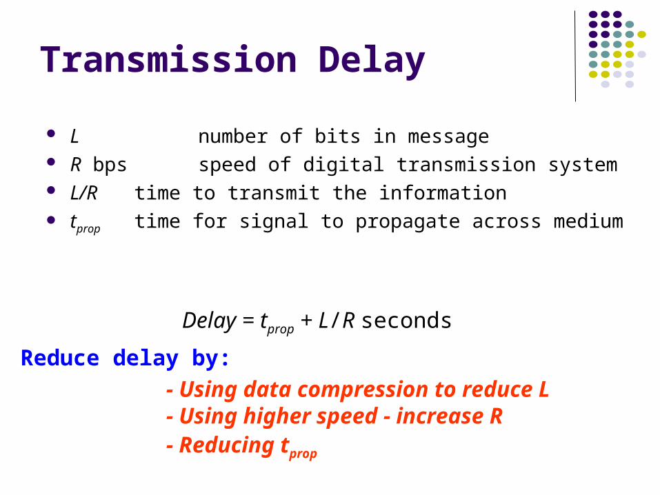
- Using data compression to reduce L- Using higher speed - increase R - Reducing tprop

L number of bits in message R bps speed of digital transmission system L/R time to transmit the information tprop time for signal to propagate across medium

Delay = tprop + L/R seconds

Reduce delay by:

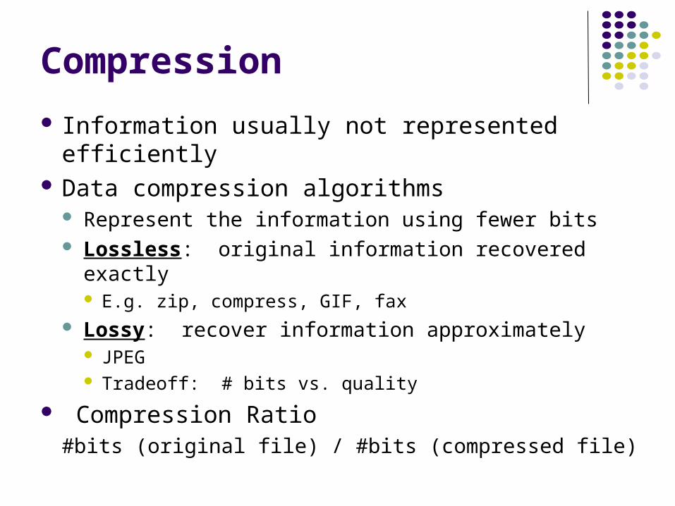
Compression

Information usually not represented efficiently Data compression algorithms

Represent the information using fewer bits Lossless: original information recovered exactly

E.g. zip, compress, GIF, fax Lossy: recover information approximately

JPEG Tradeoff: # bits vs. quality

Compression Ratio#bits (original file) / #bits (compressed file)

Data Compression Lossless Compression

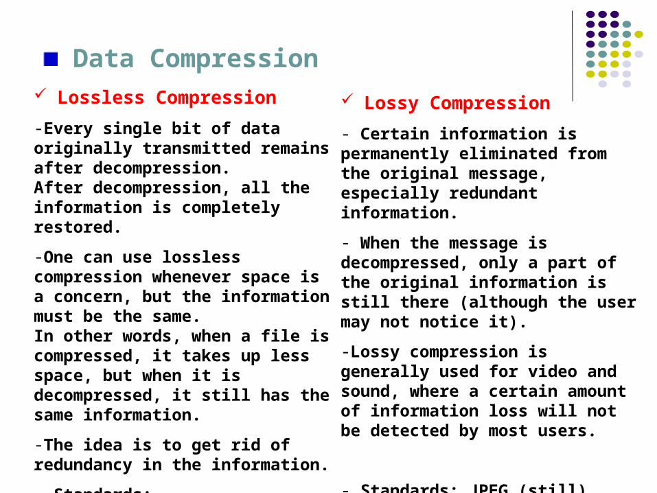
-Every single bit of data originally transmitted remains after decompression. After decompression, all the information is completely restored.

-One can use lossless compression whenever space is a concern, but the information must be the same. In other words, when a file is compressed, it takes up less space, but when it is decompressed, it still has the same information.

-The idea is to get rid of redundancy in the information.

- Standards: ZIP, GZIP, UNIX Compress, GIF

Lossy Compression

- Certain information is permanently eliminated from the original message, especially redundant information.

- When the message is decompressed, only a part of the original information is still there (although the user may not notice it).

-Lossy compression is generally used for video and sound, where a certain amount of information loss will not be detected by most users.

- Standards: JPEG (still), MPEG (audio and video), MP3 (MPEG-1 Audio Layer 3)

Lossless Compression

Background:

When we encode characters in computers, we assign each an 8-bit code based on (extended) ASCII chart.

(Extended) ASCII: fixed 8 bits per characterExample: for “hello there!” a number of 12 characters*8bits=96 bits are needed.

QUESTION: Can one encode this message using fewer bits?

Answer: Yes. In general, in most files, some characters appear most often than others. So, it makes sense to assign shorter codes for characters that appear more often, and longer codes for characters that appear less often.

This is exactly what C. Shannon and R.M. Fano were thinking when created the first compression algorithm in 1950. Huffman codes use this idea.Other coding algorithms (use different approaches): Lempel Ziv and arithmetic coding.

Lossy Compression JPEG Compression (Q=75% and 30%)

45 KB 22 KBQuality factor “Q”High quality Q = 100%Medium quality Q = 50%Poor quality Small Q

Fro

m L

iu’s

EE

330

(Pri

ncet

on)

Type Method Format Original Compressed(Ratio)

Text Zip compress

ASCII Kbytes- Mbytes

(2-6)

Fax CCITT Group 3

A4 page 200x100 pixels/in2

256 kbytes

5-54 kbytes (5-50)

Color Image

JPEG 8x10 in2 photo

4002 pixels/in2

38.4 Mbytes

1-8 Mbytes (5-30)

Examples of Block Information

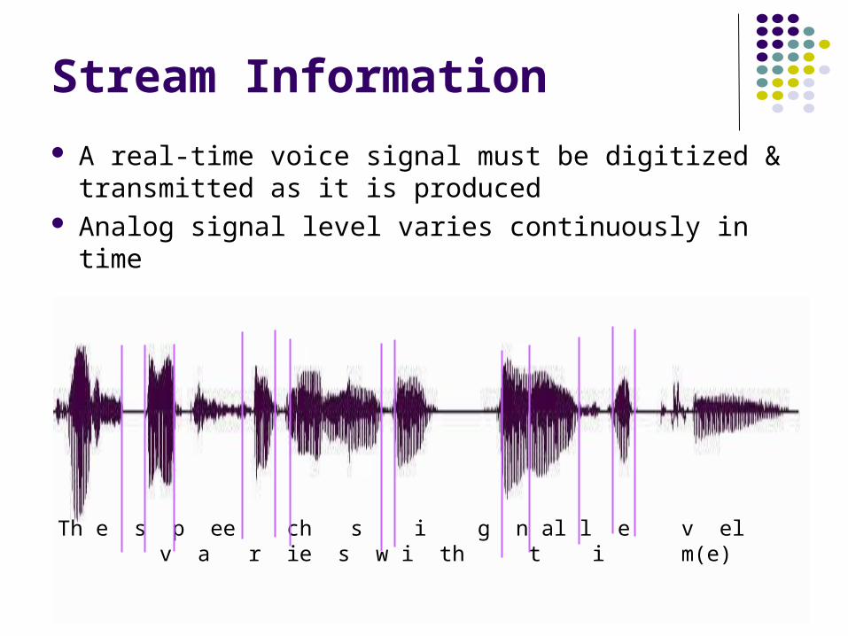
Th e s p ee ch s i g n al l e v el v a r ie s w i th t i m(e)

Stream Information

A real-time voice signal must be digitized & transmitted as it is produced

Analog signal level varies continuously in time

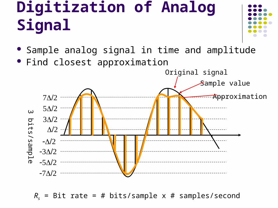
Digitization of Analog Signal

Sample analog signal in time and amplitude Find closest approximation

Original signal

Sample value

Approximation

Rs = Bit rate = # bits/sample x # samples/second

3 bits/sample

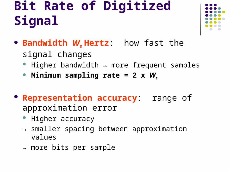
Bit Rate of Digitized Signal

Bandwidth Ws Hertz: how fast the signal changes Higher bandwidth → more frequent samples Minimum sampling rate = 2 x Ws

Representation accuracy: range of approximation error Higher accuracy

→ smaller spacing between approximation values

→ more bits per sample

Example: Voice & Audio

Telephone voice Ws = 4 kHz → 8000

samples/sec 8 bits/sample Rs=8 x 8000 = 64 kbps Cellular phones use

powerful compression algorithms

CD Audio Ws = 22 kHz → 44000

samples/sec 16 bits/sample Rs=16 x 44000= 704 kbps

per audio channel MP3 (MPEG-1 Audio

Layer 3)- powerful compression algorithms

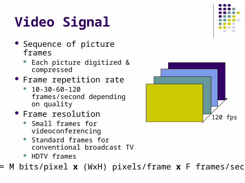
Video Signal

Sequence of picture frames Each picture digitized &

compressed Frame repetition rate

10-30-60-120 frames/second depending on quality

Frame resolution Small frames for

videoconferencing Standard frames for

conventional broadcast TV HDTV frames

120 fps

Rate = M bits/pixel x (WxH) pixels/frame x F frames/second

Video Frames

Broadcast TV at 30 frames/sec =

10.4 x 106 pixels/sec

720

480

HDTV at 30 frames/sec =

67 x 106 pixels/sec1080

1920

Videoconferencing at 30 frames/sec =

760,000 pixels/sec

144

176

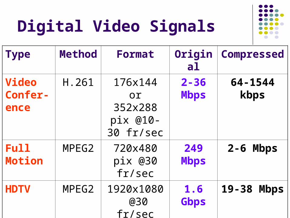
Digital Video Signals

Type Method Format Original Compressed

Video Confer-ence

H.261 176x144 or 352x288 pix

@10-30 fr/sec

2-36 Mbps

64-1544 kbps

Full Motion

MPEG2 720x480 pix @30 fr/sec

249 Mbps

2-6 Mbps

HDTV MPEG2 1920x1080 @30 fr/sec

1.6 Gbps

19-38 Mbps

Transmission of Stream Information

Constant bit-rate Signals such as digitized telephone voice produce

a steady stream: e.g. 64 kbps Network must support steady transfer of signal,

e.g. 64 kbps circuit Variable bit-rate

Signals such as digitized video produce a stream that varies in bit rate, e.g. according to motion and detail in a scene

Network must support variable transfer rate of signal, e.g., packet switching

Stream Service Quality Issues

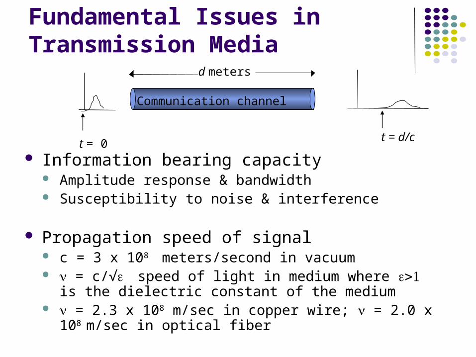
Network Transmission Impairments Delay: Is information delivered in timely

fashion? Jitter: Is information delivered in sufficiently

smooth fashion? Loss: Is information delivered without loss?

If loss occurs, is delivered signal quality acceptable?

Applications & application layer protocols developed to deal with these impairments

Communication Networks and Services

Why Digital Communications?

A Transmission System

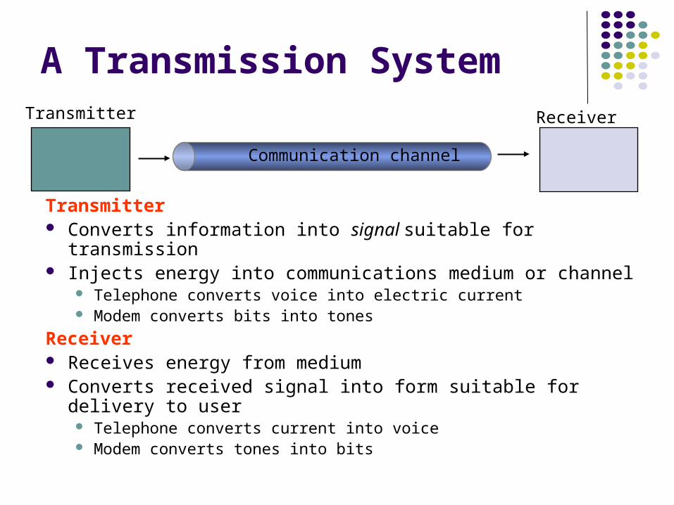
Transmitter Converts information into signal suitable for transmission Injects energy into communications medium or channel

Telephone converts voice into electric current Modem converts bits into tones

Receiver Receives energy from medium Converts received signal into form suitable for delivery to user

Telephone converts current into voice Modem converts tones into bits

Receiver

Communication channel

Transmitter

Transmission Impairments

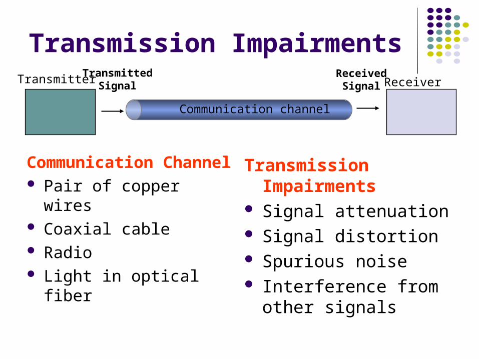
Communication Channel Pair of copper wires Coaxial cable Radio Light in optical fiber

Transmission Impairments Signal attenuation Signal distortion Spurious noise Interference from other

signals

Transmitted Signal

Received Signal Receiver

Communication channel

Transmitter

Analog Long-Distance Communications

Each repeater attempts to restore analog signal to its original form

Restoration is imperfect Distortion is not completely eliminated Noise & interference is only partially removed

Signal quality decreases with # of repeaters Communication is distance-limited Still used in analog cable TV systems Analogy: Copy a song using a cassette recorder

Source DestinationRepeater

Transmission segment

Repeater. . .

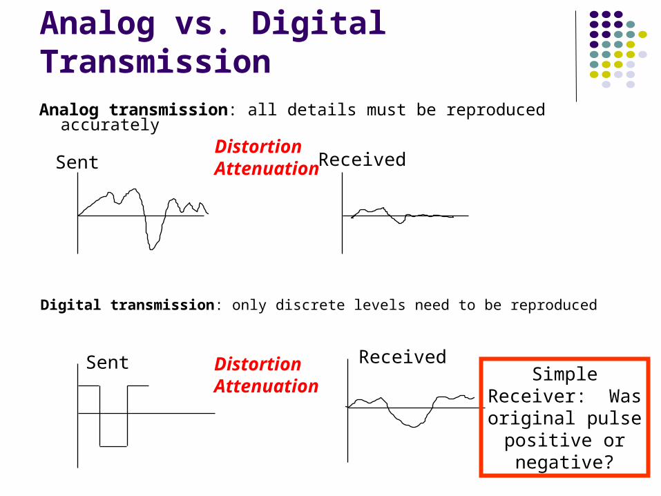
Analog vs. Digital TransmissionAnalog transmission: all details must be reproduced accurately

Sent

Sent

Received

Received

DistortionAttenuation

Digital transmission: only discrete levels need to be reproduced

DistortionAttenuation

Simple Receiver: Was original pulse

positive or negative?

Digital Long-Distance Communications

Regenerator recovers original data sequence and retransmits on next segment

Can be designed so that error probability is very small Then each regeneration is like the first time! Analogy: copy an MP3 file Communication is possible over very long distances Digital systems vs. analog systems

Less power, longer distances, lower system cost Monitoring, multiplexing, coding, encryption, protocols…

Source DestinationRegenerator

Transmission segment

Regenerator. . .

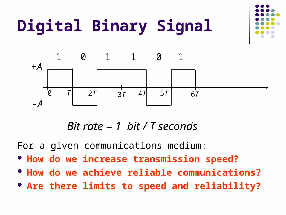
Digital Binary Signal

For a given communications medium: How do we increase transmission speed? How do we achieve reliable communications? Are there limits to speed and reliability?

+A

-A0 T 2T 3T 4T 5T 6T

1 1 1 10 0

Bit rate = 1 bit / T seconds

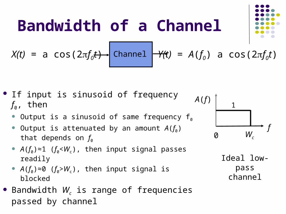
Bandwidth of a Channel

If input is sinusoid of frequency f0, then Output is a sinusoid of same frequency f0

Output is attenuated by an amount A(f0) that depends on f0

A(f0)≈1 (f0<Wc), then input signal passes readily

A(f0)≈0 (f0>Wc), then input signal is blocked

Bandwidth Wc is range of frequencies passed by channel

ChannelX(t) = a cos(2f0t) Y(t) = A(f0) a cos(2f0t)

Wc0f

A(f)1

Ideal low-pass channel

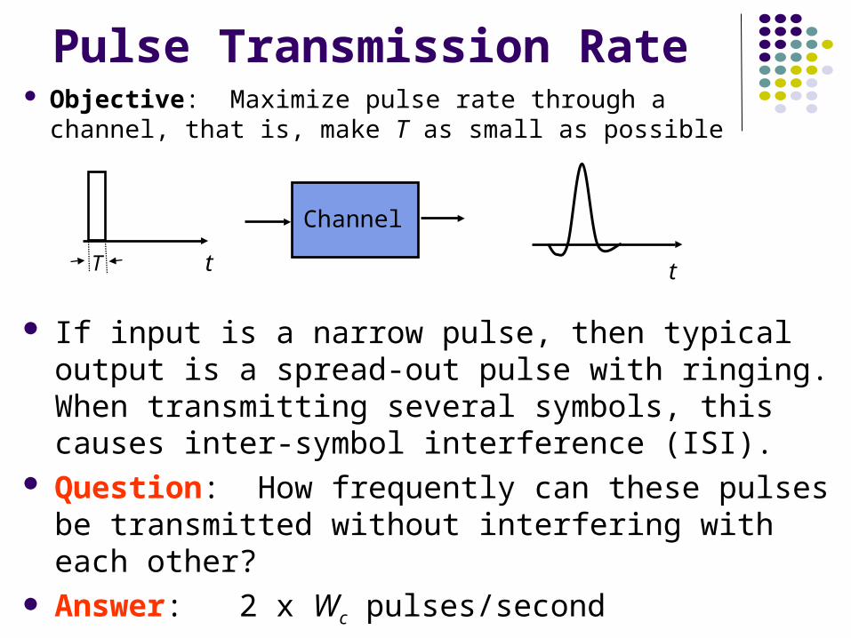
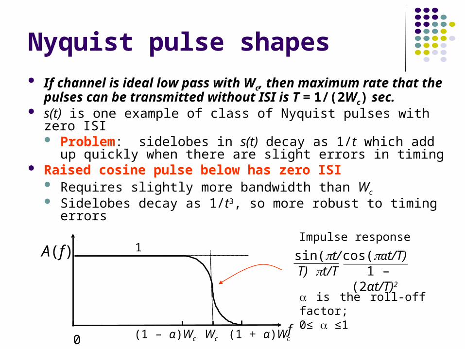
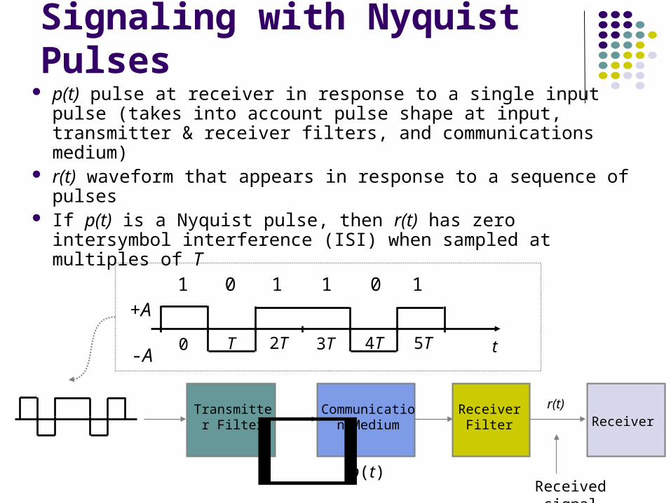
Pulse Transmission Rate Objective: Maximize pulse rate through a

channel, that is, make T as small as possible

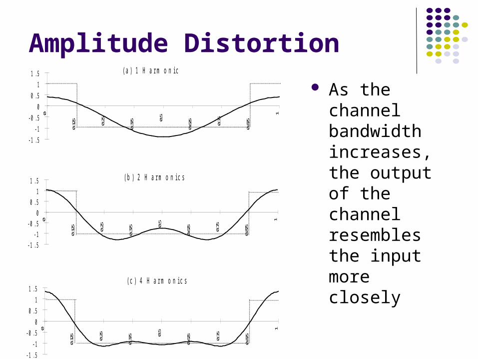
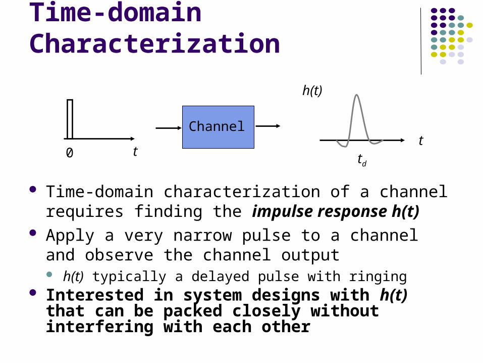
If input is a narrow pulse, then typical output is a spread-out pulse with ringing. When transmitting several symbols, this causes inter-symbol interference (ISI).

Question: How frequently can these pulses be transmitted without interfering with each other?

Answer: 2 x Wc pulses/second

where Wc is the bandwidth of the channel

Channel

t tT

Multilevel Pulse Transmission

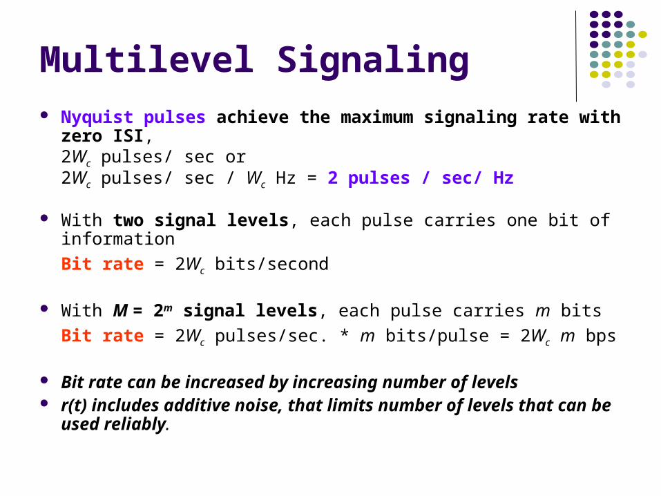
Assume channel of bandwidth Wc, and transmit 2 Wc pulses/sec (without interference)

If pulses amplitudes are either -A or +A, then each pulse conveys 1 bit, so

Bit Rate = 1 bit/pulse x 2Wc pulses/sec = 2Wc bps If amplitudes are from {-A, -A/3, +A/3, +A}, then bit

rate is 2 x 2Wc bps By going to M = 2m amplitude levels, we achieve

Bit Rate = m bits/pulse x 2Wc pulses/sec = 2mWc bps

In the absence of noise, the bit rate can be increased without limit by increasing m

Noise & Reliable Communications

All physical systems have noise Electrons always vibrate at non-zero temperature Motion of electrons induces noise

Presence of noise limits accuracy of measurement of received signal amplitude

Errors occur if signal separation is comparable to noise level

Bit Error Rate (BER) increases with decreasing signal-to-noise ratio

Noise places a limit on how many amplitude levels can be used in pulse transmission

SNR = Average signal power

Average noise power

SNR (dB) = 10 log10 SNR

Signal Noise Signal + noise

Signal Noise Signal + noise

HighSNR

LowSNR

t t t

t t t

Signal-to-Noise Ratio

error

No errors

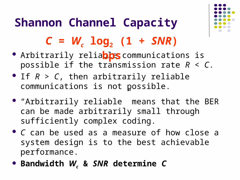
Arbitrarily reliable communications is possible if the transmission rate R < C.

If R > C, then arbitrarily reliable communications is not possible.

“Arbitrarily reliable” means that the BER can be made arbitrarily small through sufficiently complex coding.

C can be used as a measure of how close a system design is to the best achievable performance.

Bandwidth Wc & SNR determine C

Shannon Channel Capacity

C = Wc log2 (1 + SNR) bps

Example

Find the Shannon channel capacity for a telephone channel with Wc = 3400 Hz and SNR = 10000

C = 3400 log2 (1 + 10000)

= 3400 log10 (10001)/log102 = 45200 bps

Note that SNR = 10000 corresponds to

SNR (dB) = 10 log10(10000) = 40 dB

Bit Rates of Digital Transmission Systems

System Bit Rate Observations

Telephone twisted pair

33.6-56 kbps 4 kHz telephone channel

Ethernet twisted pair

10 Mbps, 100 Mbps 100 meters of unshielded twisted copper wire pair

Cable modem 500 kbps-4 Mbps Shared CATV return channel

ADSL twisted pair

64-640 kbps in, 1.536-6.144 Mbps out

Coexists with analog telephone signal

2.4 GHz radio 2-11 Mbps IEEE 802.11 wireless LAN

28 GHz radio 1.5-45 Mbps 5 km multipoint radio

Optical fiber 2.5-10 Gbps 1 wavelength

Optical fiber >1600 Gbps Many wavelengths

Examples of Channels

Channel Bandwidth Bit Rates

Telephone voice channel

3 kHz 33 kbps

Copper pair 1 MHz 1-6 Mbps

Coaxial cable 500 MHz (6 MHz channels)

30 Mbps/ channel

5 GHz radio (IEEE 802.11)

300 MHz (11 channels)

54 Mbps / channel

Optical fiber Many Tera Hertz 40 Gbps / wavelength

Digital Transmission Fundamentals

Signal Time Variations And Bandwidth

Sampling Rate and Bandwidth

A signal that varies faster needs to be sampled more frequently

Bandwidth measures how fast a signal varies

What is the bandwidth of these signals?

1 ms

. . . . . .

t

x2(t)

. . . . . .

t

1 ms

x1(t)

Periodic Signals

A periodic signal with period T can be represented as sum of sinusoids using Fourier Series:

“DC” long-term average

fundamental frequency f0=1/T

first harmonic

kth harmonic

x(t) = a0 + a1cos(2f0t + 1) + a2cos(22f0t + 2) + …

+ akcos(2kf0t + k) + …

•|ak| determines amount of power in kth harmonic

•Amplitude specturm |a0|, |a1|, |a2|, …

Example Fourier Series

T1 = 1 ms

1 1 1 1 0 0 0 0

. . . . . .

t

x2(t)1 0 1 0 1 0 1 0

. . . . . .

t

T2 =0.25 ms

x1(t)

Only odd harmonics have power

x1(t) = 0 + cos(24000t)

+ cos(23(4000)t)

+ cos(25(4000)t) + …

4

4 5

4 3

x2(t) = 0 + cos(21000t)

+ cos(23(1000)t)

+ cos(25(1000)t) + …

4

4 5

4 3

Spectra & Bandwidth

Spectrum of a signal: magnitude of amplitudes as a function of frequency

x1(t) varies faster in time & has more high frequency content than x2(t)

Bandwidth Ws is defined as range of frequencies where a signal has non-negligible power, e.g. range of band that contains 99% of total signal power

0

0.2

0.4

0.6

0.8

1

1.2

0 3 6 9 12 15 18 21 24 27 30 33 36 39 42

frequency (kHz)

0

0.2

0.4

0.6

0.8

1

1.2

0 3 6 9 12 15 18 21 24 27 30 33 36 39 42

frequency (kHz)

Spectrum of x1(t)

Spectrum of x2(t)

Bandwidth of General Signals

Not all signals are periodic E.g. voice signals varies

according to sound Vowels are periodic, “s” is

noiselike Spectrum of long-term signal

Averages over many sounds, many speakers

Involves Fourier transform Telephone speech: 4 kHz CD Audio: 22 kHz

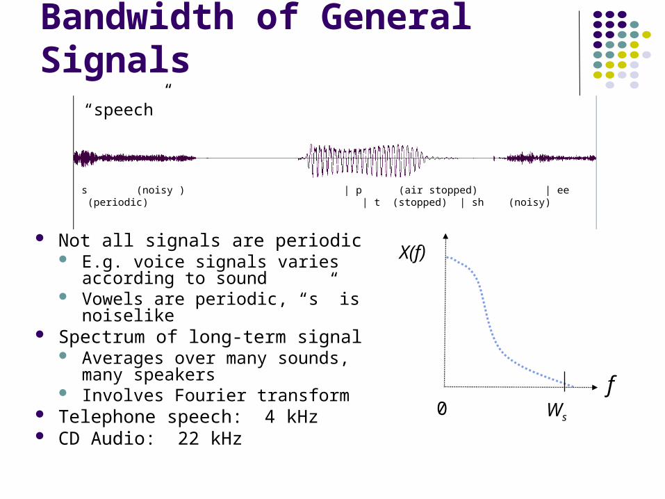
s (noisy ) | p (air stopped) | ee (periodic) | t (stopped) | sh (noisy)

X(f)

f0 Ws

“speech”

Digital Transmission Fundamentals

Characterization of Communication Channels

Communications Channels A physical medium is an inherent part of a

communications system Copper wires, radio medium, or optical fiber

Communications system includes electronic or optical devices that are part of the path followed by a signal Equalizers, amplifiers, signal conditioners

By communication channel we refer to the combined end-to-end physical medium and attached devices

Sometimes we use the term filter to refer to a channel especially in the context of a specific mathematical model for the channel

How good is a channel?

Performance: What is the maximum reliable transmission speed? Speed: Bit rate, R bps Reliability: Bit error rate, BER=10-k

Cost: What is the cost of alternatives at a given level of performance? Wired vs. wireless? Electronic vs. optical? Standard A vs. standard B?

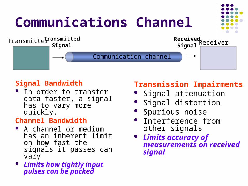
Communications Channel

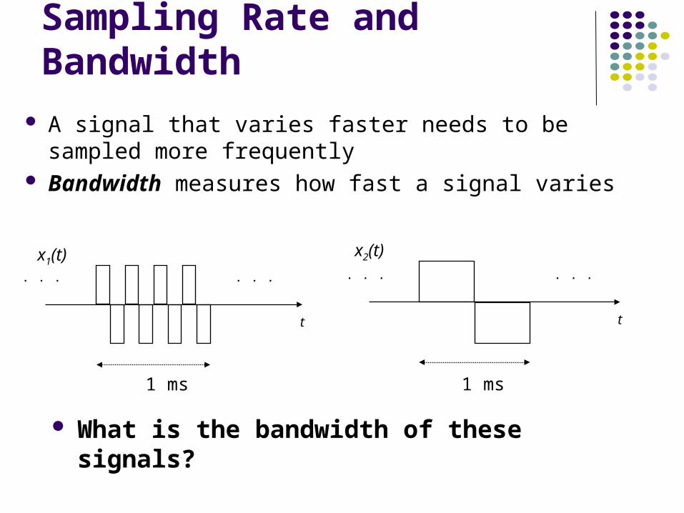
Signal Bandwidth In order to transfer data

faster, a signal has to vary more quickly.

Channel Bandwidth A channel or medium has

an inherent limit on how fast the signals it passes can vary

Limits how tightly input pulses can be packed

Transmission Impairments Signal attenuation Signal distortion Spurious noise Interference from other

signals Limits accuracy of

measurements on received signal

Transmitted Signal

Received Signal Receiver

Communication channel

Transmitter

Channel

t t

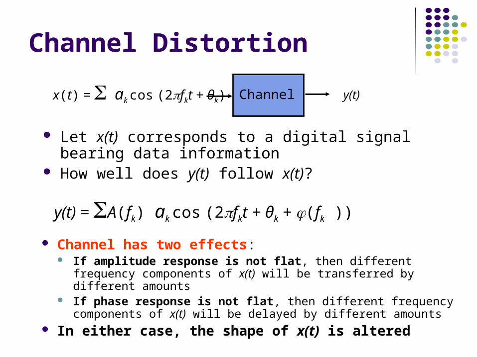
x(t)= Aincos 2f0t y(t)=Aoutcos (2f0t + (f0))

Aout

AinA(f0) =

Frequency Domain Channel Characterization

Apply sinusoidal input at frequency f0 Output is sinusoid at same frequency, but attenuated & phase-shifted Measure amplitude of output sinusoid (of same frequency f0) Calculate amplitude response

A(f0) = ratio of output amplitude to input amplitude If A(f0) ≈ 1, then input signal passes readily If A(f0) ≈ 0, then input signal is blocked

Bandwidth Wc is range of frequencies passed by channel

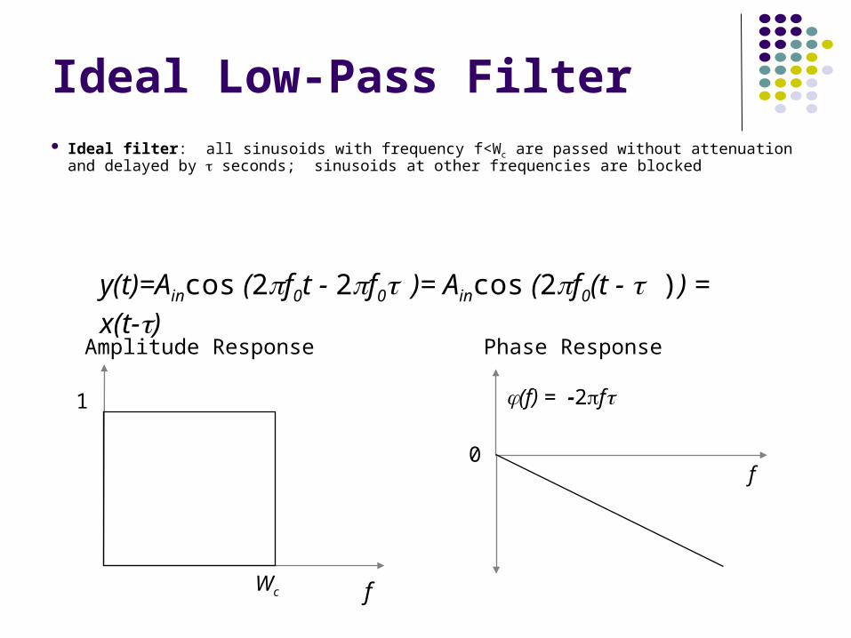
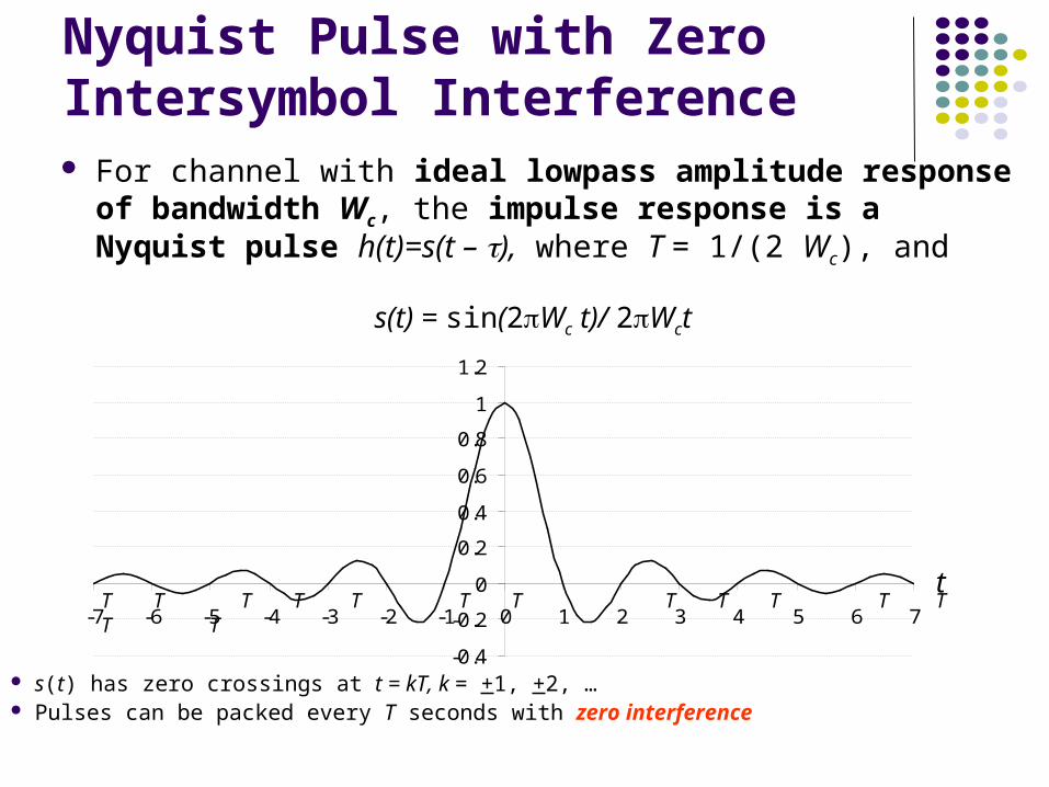
Ideal Low-Pass Filter Ideal filter: all sinusoids with frequency f<Wc are passed without attenuation and

delayed by seconds; sinusoids at other frequencies are blocked

Amplitude Response

f

1

f0

(f) = -2f

Phase Response

Wc

y(t)=Aincos (2f0t - 2f0 )= Aincos (2f0(t - )) = x(t-)

Example: Low-Pass Filter Simplest non-ideal circuit that provides low-pass filtering

Inputs at different frequencies are attenuated by different amounts Inputs at different frequencies are delayed by different amounts

f

1 A(f) = 1

(1+42f2)1/2

Amplitude Response

f0

(f) = tan-1 2f

-45o

-90o

1/ 2

Phase Response

Channel Distortion

Channel has two effects: If amplitude response is not flat, then different frequency

components of x(t) will be transferred by different amounts If phase response is not flat, then different frequency

components of x(t) will be delayed by different amounts In either case, the shape of x(t) is altered

Let x(t) corresponds to a digital signal bearing data information

How well does y(t) follow x(t)?

y(t) = A(fk) ak cos (2fkt + θk + (fk ))

Channel y(t)x(t) = ak cos (2fkt + θk)

Example: Amplitude Distortion

Let x(t) input to ideal lowpass filter that has zero delay and Wc = 1.5 kHz, 2.5 kHz, or 4.5 kHz

1 0 0 0 0 0 0 1

. . . . . .

t1 ms

x(t)

Wc = 1.5 kHz passes only the first two terms

Wc = 2.5 kHz passes the first three terms

Wc = 4.5 kHz passes the first five terms

x(t) = -0.5 + sin( )cos(21000t)

+ sin( )cos(22000t) + sin( )cos(23000t) + …

4

4

4

4

2 4

3 4

- 1 . 5

- 1

- 0 . 5

0

0 . 5

1

1 . 5

0

0.125 0.2

5

0.375 0.5

0.625 0.7

5

0.875

1

- 1 . 5

- 1

- 0 . 5

0

0 . 5

1

1 . 5

0

0.125 0.2

5

0.375 0.5

0.625 0.7

5

0.875

1

- 1 . 5

- 1

- 0 . 5

0

0 . 5

1

1 . 5

0

0.125 0.2

5

0.375 0.5

0.625 0.7

5

0.875

1

( b ) 2 H a r m o n i c s

( c ) 4 H a r m o n i c s

( a ) 1 H a r m o n i c

Amplitude Distortion

As the channel bandwidth increases, the output of the channel resembles the input more closely

Channel

t0t

h(t)

td

Time-domain Characterization

Time-domain characterization of a channel requires finding the impulse response h(t)

Apply a very narrow pulse to a channel and observe the channel output h(t) typically a delayed pulse with ringing

Interested in system designs with h(t) that can be packed closely without interfering with each other

Nyquist Pulse with Zero Intersymbol Interference For channel with ideal lowpass amplitude response of

bandwidth Wc, the impulse response is a Nyquist pulse h(t)=s(t – ), where T = 1/(2 Wc), and

-0.4

-0.2

0

0.2

0.4

0.6

0.8

1

1.2

-7 -6 -5 -4 -3 -2 -1 0 1 2 3 4 5 6 7t

s(t) = sin(2Wc t)/ 2Wct

T T T T T T T T T T T T T T

s(t) has zero crossings at t = kT, k = +1, +2, … Pulses can be packed every T seconds with zero interference

-2

-1

0

1

2

-2 -1 0 1 2 3 4t

T T T T TT

-1

0

1

-2 -1 0 1 2 3 4t

T T T T TT

Example of composite waveform

Three Nyquist pulses shown separately

+ s(t) + s(t-T) - s(t-2T)Composite waveformr(t) = s(t)+s(t-T)-s(t-2T)Samples at kTr(0)=s(0)+s(-T)-s(-2T)=+1r(T)=s(T)+s(0)-s(-T)=+1r(2T)=s(2T)+s(T)-s(0)=-1

Zero intersymbol interference (ISI) at sampling times kT

r(t)

+s(t) +s(t-T)

-s(t-2T)

0f

A(f)

Nyquist pulse shapes If channel is ideal low pass with Wc, then maximum rate

that the pulses can be transmitted without ISI is T = 1/(2Wc) sec.

s(t) is one example of class of Nyquist pulses with zero ISI Problem: sidelobes in s(t) decay as 1/t which add up

quickly when there are slight errors in timing Raised cosine pulse below has zero ISI

Requires slightly more bandwidth than Wc Sidelobes decay as 1/t3, so more robust to timing errors

1sin(t/T)

t/Tcos(αt/T) 1 – (2αt/T)2

(1 – α)Wc Wc (1 + α)Wc

is the roll-off factor;0≤ ≤1

Impulse response

Digital Transmission Fundamentals

Fundamental Limits in Digital Transmission

Transmitter Filter

Communication Medium

Receiver Filter Receiver

r(t)

Received signal

+A

-A0 T 2T 3T 4T 5T

1 1 1 10 0

t

Signaling with Nyquist Pulses p(t) pulse at receiver in response to a single input pulse

(takes into account pulse shape at input, transmitter & receiver filters, and communications medium)

r(t) waveform that appears in response to a sequence of pulses

If p(t) is a Nyquist pulse, then r(t) has zero intersymbol interference (ISI) when sampled at multiples of T

p(t)

Multilevel Signaling Nyquist pulses achieve the maximum signaling rate with zero

ISI, 2Wc pulses/ sec or 2Wc pulses/ sec / Wc Hz = 2 pulses / sec/ Hz

With two signal levels, each pulse carries one bit of information

Bit rate = 2Wc bits/second

With M = 2m signal levels, each pulse carries m bits

Bit rate = 2Wc pulses/sec. * m bits/pulse = 2Wc m bps

Bit rate can be increased by increasing number of levels r(t) includes additive noise, that limits number of levels that

can be used reliably.

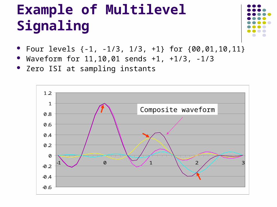
Example of Multilevel Signaling

Four levels {-1, -1/3, 1/3, +1} for {00,01,10,11} Waveform for 11,10,01 sends +1, +1/3, -1/3 Zero ISI at sampling instants

-0.6

-0.4

-0.2

0

0.2

0.4

0.6

0.8

1

1.2

-1 0 1 2 3

Composite waveform

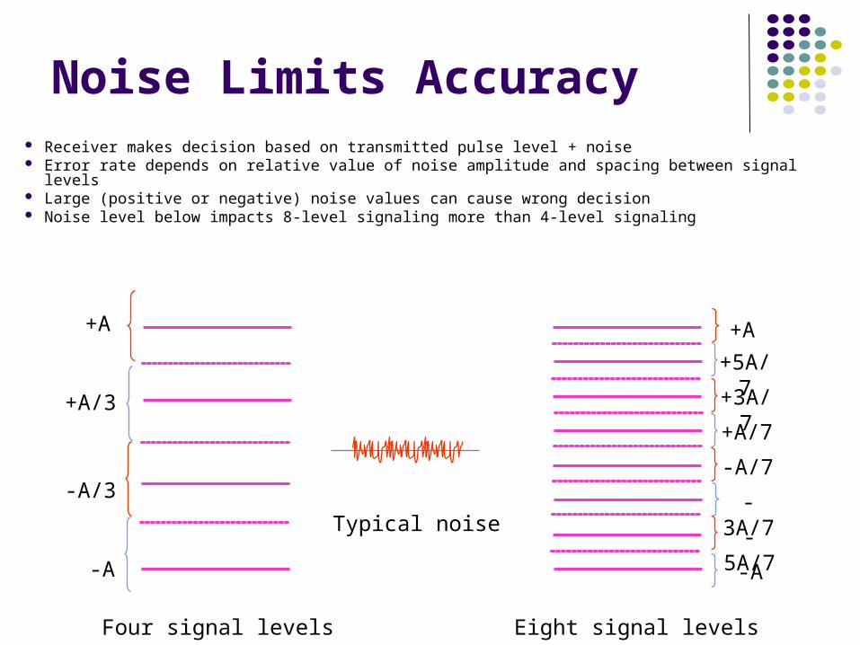
Four signal levels Eight signal levels

Typical noise

Noise Limits Accuracy Receiver makes decision based on transmitted pulse level + noise Error rate depends on relative value of noise amplitude and spacing between signal levels Large (positive or negative) noise values can cause wrong decision Noise level below impacts 8-level signaling more than 4-level signaling

+A

+A/3

-A/3

-A

+A

+5A/7

+3A/7

+A/7

-A/7

-3A/7

-5A/7

-A

222

2

1

xe

x0

Noise distribution Noise is characterized by probability density of amplitude samples Likelihood that certain amplitude occurs Thermal electronic noise is inevitable (due to vibrations of electrons) Noise distribution is Gaussian (bell-shaped) as below

t

x

Pr[X(t)>x0 ] = ?

Pr[X(t)>x0 ] =Area under

graph

x0

x0

= Avg Noise Power

1.00E-121.00E-111.00E-101.00E-091.00E-081.00E-071.00E-061.00E-051.00E-041.00E-031.00E-021.00E-011.00E+00

0 2 4 6 8 /2

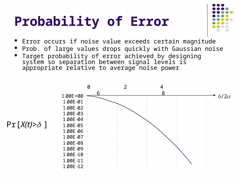
Probability of Error Error occurs if noise value exceeds certain magnitude Prob. of large values drops quickly with Gaussian noise Target probability of error achieved by designing system so

separation between signal levels is appropriate relative to average noise power

Pr[X(t)> ]

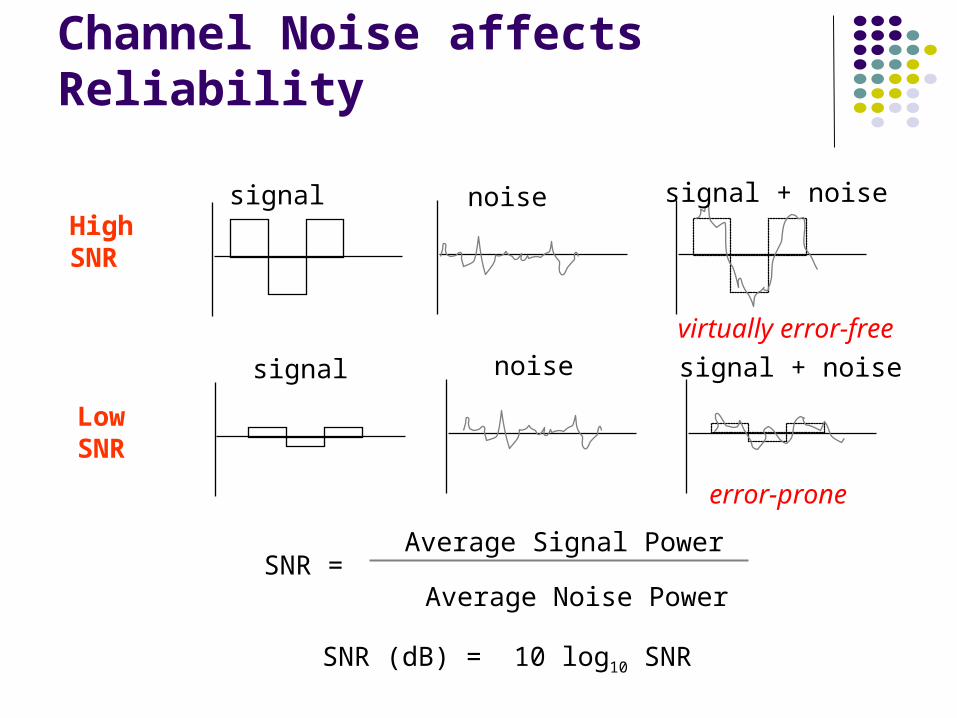
signal noise signal + noise

signal noise signal + noise

HighSNR

LowSNR

SNR = Average Signal Power

Average Noise Power

SNR (dB) = 10 log10 SNR

virtually error-free

error-prone

Channel Noise affects Reliability

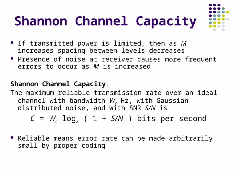
If transmitted power is limited, then as M increases spacing between levels decreases

Presence of noise at receiver causes more frequent errors to occur as M is increased

Shannon Channel Capacity:The maximum reliable transmission rate over an ideal channel with

bandwidth Wc Hz, with Gaussian distributed noise, and with SNR S/N is

C = Wc log2 ( 1 + S/N ) bits per second

Reliable means error rate can be made arbitrarily small by proper coding

Shannon Channel Capacity

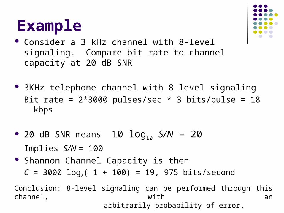
Example Consider a 3 kHz channel with 8-level signaling.

Compare bit rate to channel capacity at 20 dB SNR

3KHz telephone channel with 8 level signaling

Bit rate = 2*3000 pulses/sec * 3 bits/pulse = 18 kbps

20 dB SNR means 10 log10 S/N = 20

Implies S/N = 100 Shannon Channel Capacity is then

C = 3000 log2( 1 + 100) = 19, 975 bits/second

Conclusion: 8-level signaling can be performed through this channel, with an arbitrarily probability of error.

Digital Transmission Fundamentals

Line Coding

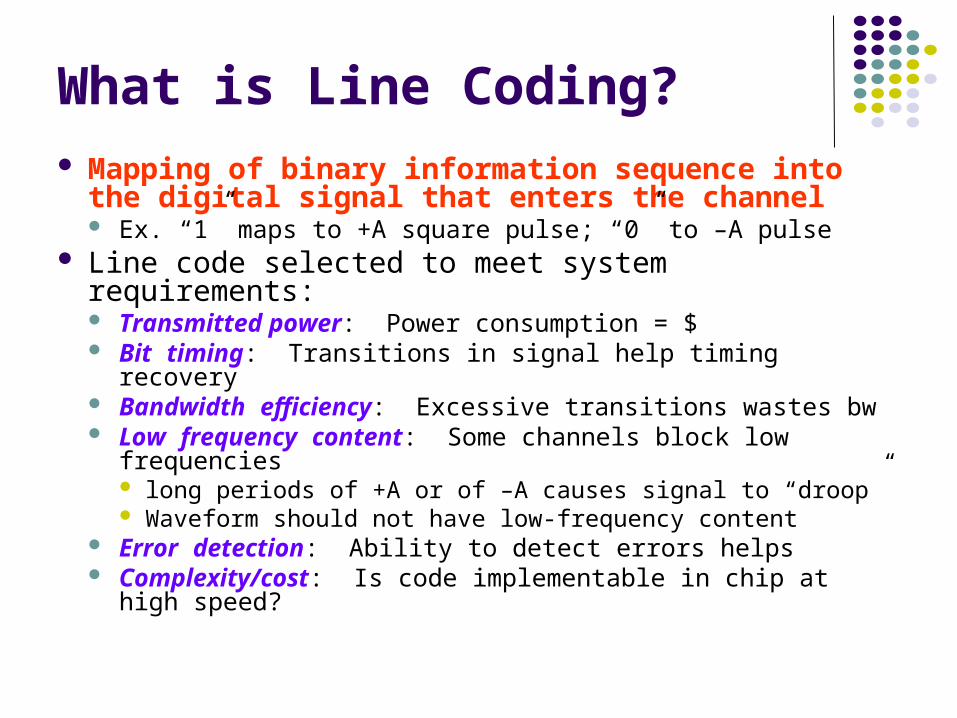
What is Line Coding? Mapping of binary information sequence into the

digital signal that enters the channel Ex. “1” maps to +A square pulse; “0” to –A pulse

Line code selected to meet system requirements: Transmitted power: Power consumption = $ Bit timing: Transitions in signal help timing recovery Bandwidth efficiency: Excessive transitions wastes bw Low frequency content: Some channels block low

frequencies long periods of +A or of –A causes signal to “droop” Waveform should not have low-frequency content

Error detection: Ability to detect errors helps Complexity/cost: Is code implementable in chip at high

speed?

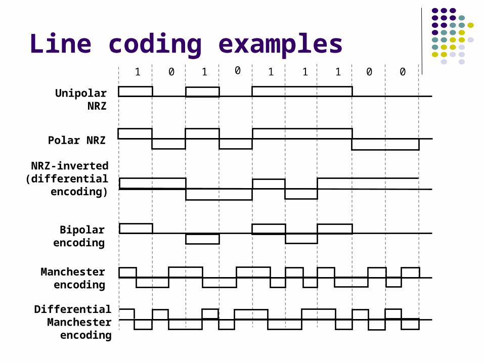
Line coding examples

NRZ-inverted(differential

encoding)

1 0 1 0 1 1 0 01

UnipolarNRZ

Bipolarencoding

Manchesterencoding

DifferentialManchester

encoding

Polar NRZ

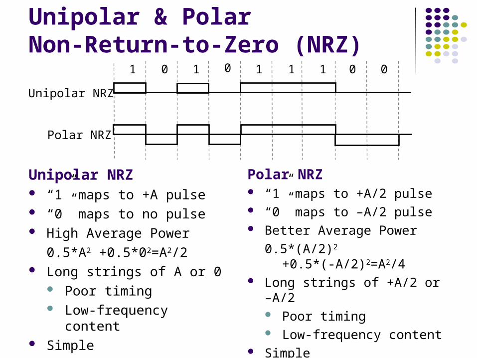
Unipolar & Polar Non-Return-to-Zero (NRZ)

Unipolar NRZ “1” maps to +A pulse “0” maps to no pulse High Average Power

0.5*A2 +0.5*02=A2/2 Long strings of A or 0

Poor timing Low-frequency content

Simple

Polar NRZ “1” maps to +A/2 pulse “0” maps to –A/2 pulse Better Average Power

0.5*(A/2)2 +0.5*(-A/2)2=A2/4 Long strings of +A/2 or –A/2

Poor timing Low-frequency content

Simple

1 0 1 0 1 1 0 01

Unipolar NRZ

Polar NRZ

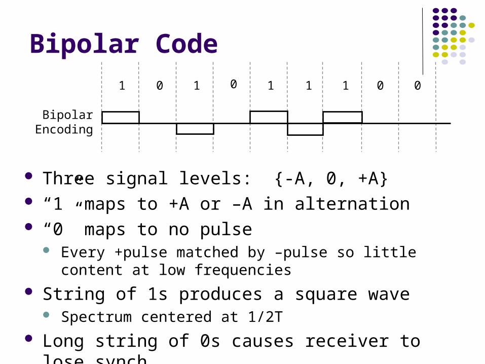
Bipolar Code

Three signal levels: {-A, 0, +A} “1” maps to +A or –A in alternation “0” maps to no pulse

Every +pulse matched by –pulse so little content at low frequencies

String of 1s produces a square wave Spectrum centered at 1/2T

Long string of 0s causes receiver to lose synch

1 0 1 0 1 1 0 01

Bipolar Encoding

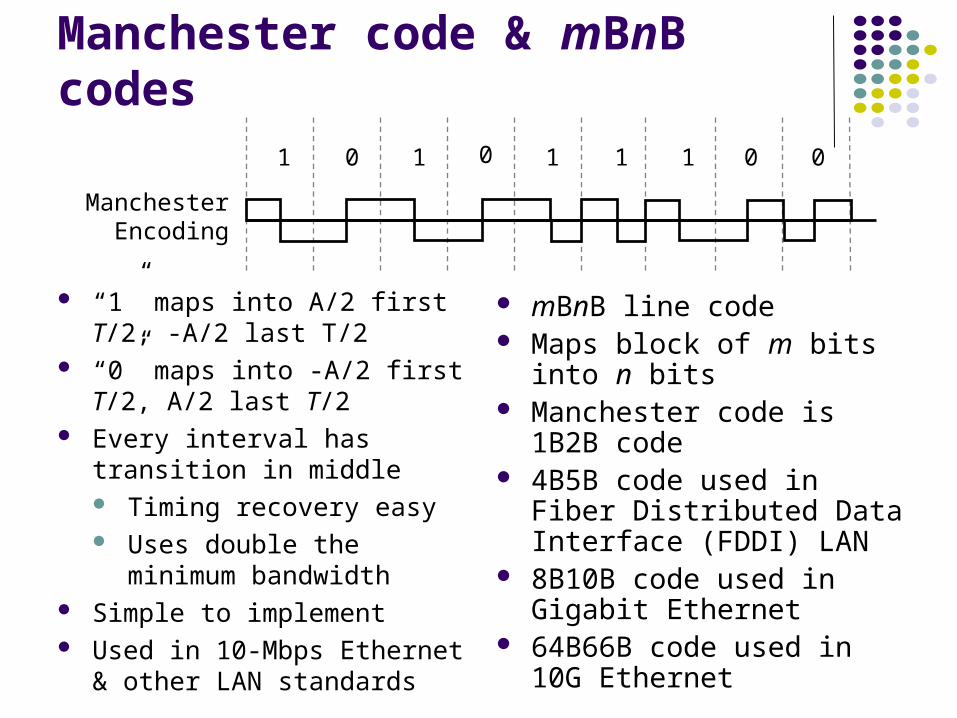
Manchester code & mBnB codes

“1” maps into A/2 first T/2, -A/2 last T/2

“0” maps into -A/2 first T/2, A/2 last T/2

Every interval has transition in middle Timing recovery easy Uses double the minimum

bandwidth Simple to implement Used in 10-Mbps Ethernet &

other LAN standards

mBnB line code Maps block of m bits into n

bits Manchester code is 1B2B

code 4B5B code used in Fiber

Distributed Data Interface (FDDI) LAN

8B10B code used in Gigabit Ethernet

64B66B code used in 10G Ethernet

1 0 1 0 1 1 0 01

Manchester Encoding

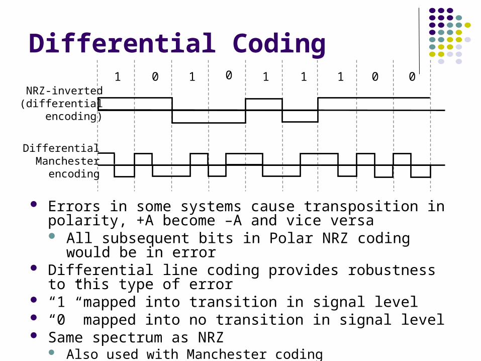
Differential Coding

Errors in some systems cause transposition in polarity, +A become –A and vice versa All subsequent bits in Polar NRZ coding would be in error

Differential line coding provides robustness to this type of error

“1” mapped into transition in signal level “0” mapped into no transition in signal level Same spectrum as NRZ

Also used with Manchester coding

NRZ-inverted(differential

encoding)

1 0 1 0 1 1 0 01

DifferentialManchester

encoding

-0.2

0

0.2

0.4

0.6

0.8

1

1.2

0

0.2

0.4

0.6

0.8 1

1.2

1.4

1.6

1.8 2

fT

pow

er d

ensi

ty

NRZ

Bipolar

Manchester

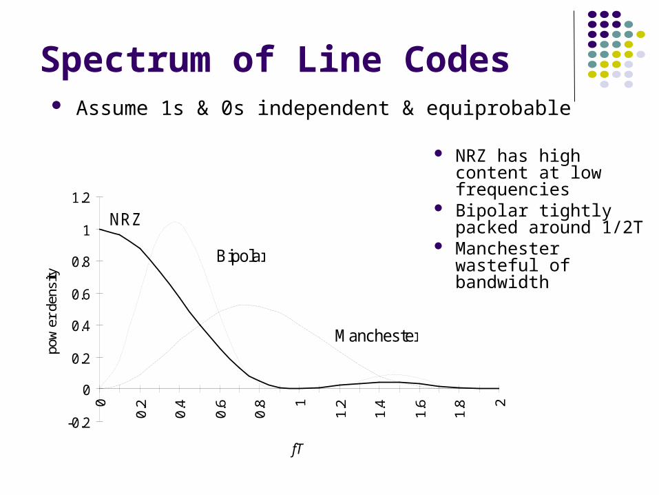
Spectrum of Line Codes Assume 1s & 0s independent & equiprobable

NRZ has high content at low frequencies

Bipolar tightly packed around 1/2T

Manchester wasteful of bandwidth

Digital Transmission Fundamentals

Modems and Digital Modulation

Bandpass Channel

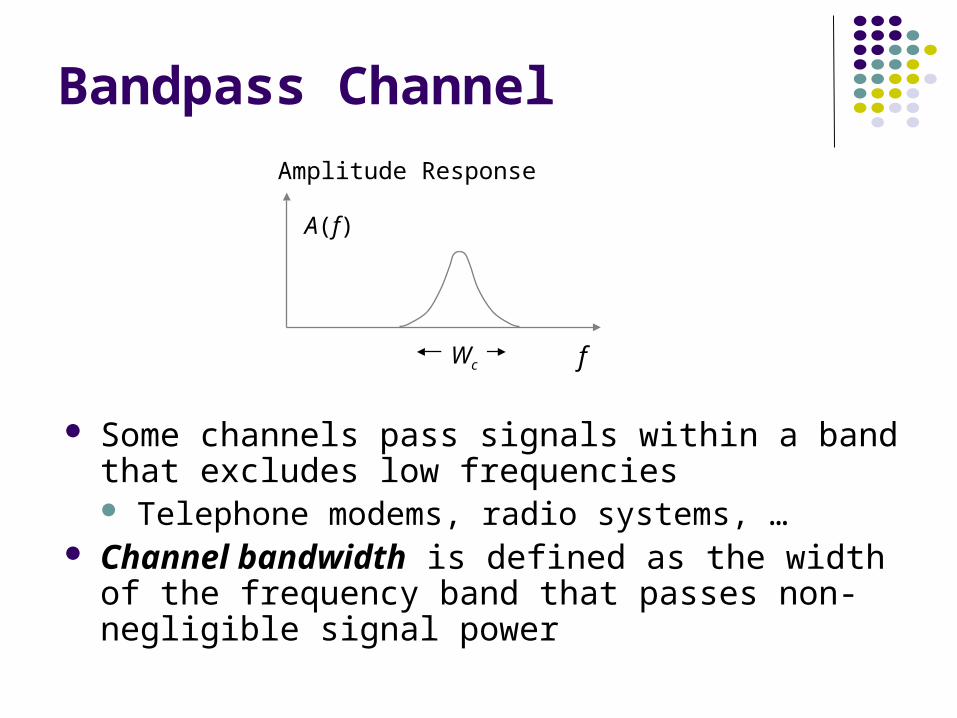
Some channels pass signals within a band that excludes low frequencies Telephone modems, radio systems, …

Channel bandwidth is defined as the width of the frequency band that passes non-negligible signal power

f

Amplitude Response

A(f)

Wc

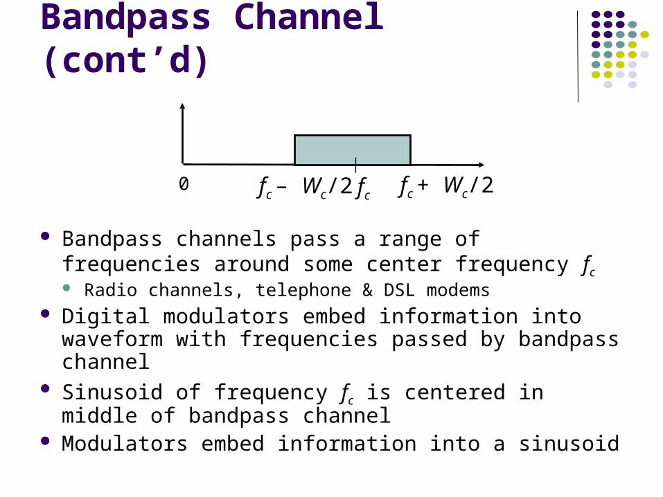
Bandpass Channel (cont’d)

Bandpass channels pass a range of frequencies around some center frequency fc Radio channels, telephone & DSL modems

Digital modulators embed information into waveform with frequencies passed by bandpass channel

Sinusoid of frequency fc is centered in middle of bandpass channel

Modulators embed information into a sinusoid

fc – Wc/2 fc0 fc + Wc/2

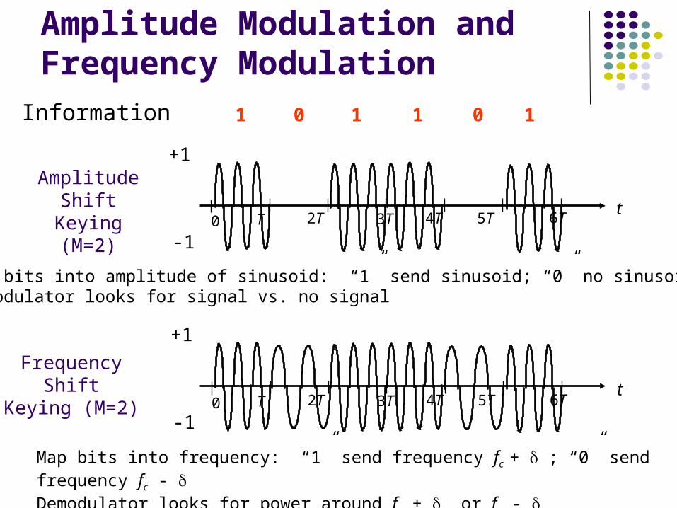
Information 1 1 1 10 0

+1

-10 T 2T 3T 4T 5T 6T

AmplitudeShift

Keying (M=2)

+1

-1

FrequencyShift

Keying (M=2) 0 T 2T 3T 4T 5T 6T

t

t

Amplitude Modulation and Frequency Modulation

Map bits into amplitude of sinusoid: “1” send sinusoid; “0” no sinusoidDemodulator looks for signal vs. no signal

Map bits into frequency: “1” send frequency fc + ; “0” send frequency fc - Demodulator looks for power around fc + or fc -

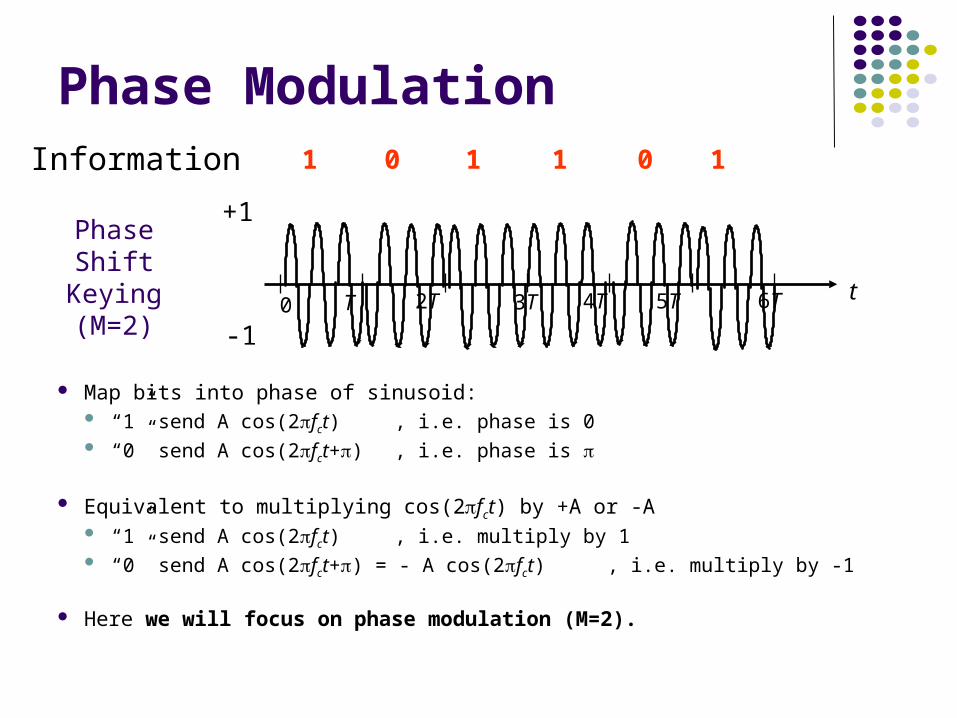
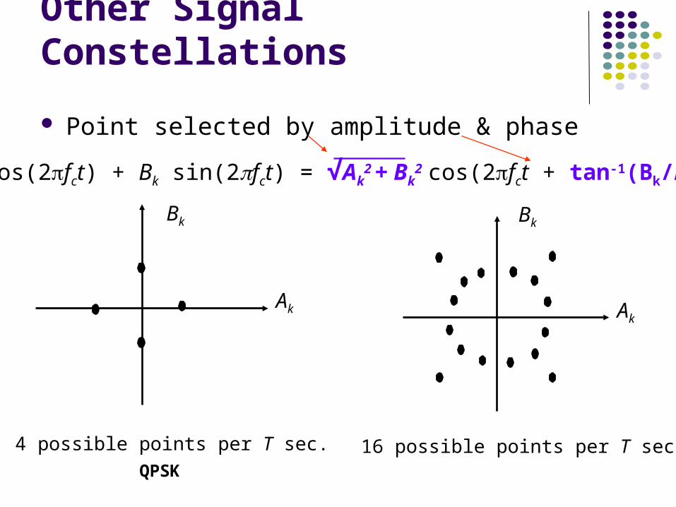
Phase Modulation

Map bits into phase of sinusoid: “1” send A cos(2fct) , i.e. phase is 0 “0” send A cos(2fct+) , i.e. phase is

Equivalent to multiplying cos(2fct) by +A or -A “1” send A cos(2fct) , i.e. multiply by 1 “0” send A cos(2fct+) = - A cos(2fct) , i.e. multiply by -1

Here we will focus on phase modulation (M=2).

+1

-1

PhaseShift

Keying (M=2) 0 T 2T 3T 4T 5T 6T t

Information 1 1 1 10 0

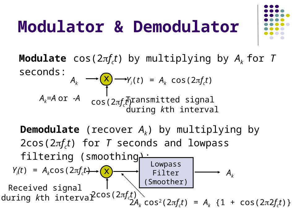
Modulate cos(2fct) by multiplying by Ak for T seconds:

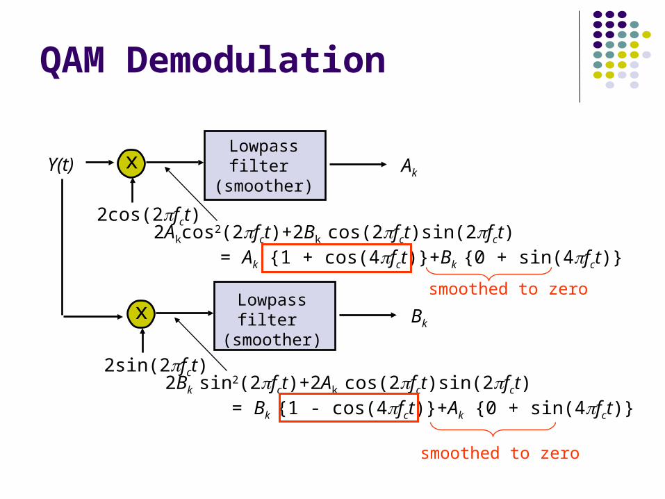
Demodulate (recover Ak) by multiplying by 2cos(2fct) for T seconds and lowpass filtering (smoothing):

x

2cos(2fct)2Ak cos2(2fct) = Ak {1 + cos(22fct)}

LowpassFilter

(Smoother)Ak

Yi(t) = Akcos(2fct)

Received signal during kth interval

Modulator & Demodulator

Akx

cos(2fct)

Yi(t) = Ak cos(2fct)

Transmitted signal during kth interval

Ak=A or -A

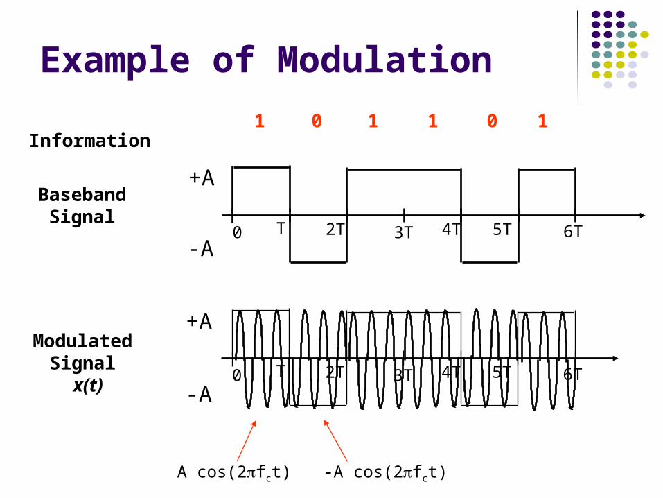
+A

-A0 T 2T 3T 4T 5T 6T

Information

BasebandSignal

ModulatedSignal

x(t)

+A

-A0 T 2T 3T 4T 5T 6T

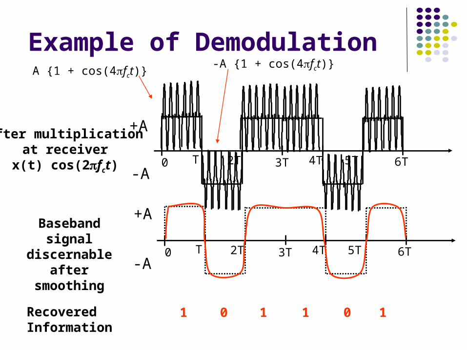
Example of Modulation

A cos(2fct) -A cos(2fct)

1 1 1 10 0

RecoveredInformation

Basebandsignal

discernable after smoothing

After multiplicationat receiver

x(t) cos(2fct)

+A

-A0 T 2T 3T 4T 5T 6T

+A

-A0 T 2T 3T 4T 5T 6T

Example of DemodulationA {1 + cos(4fct)}

-A {1 + cos(4fct)}

1 1 1 10 0

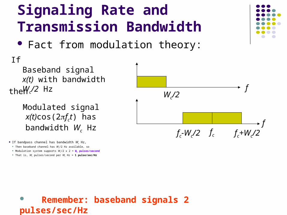
Signaling Rate and Transmission Bandwidth Fact from modulation theory:

Baseband signal x(t) with bandwidth Wc/2 Hz

If

then Wc/2

fc+Wc/2

f

ffc-Wc/2 fc

Modulated signal x(t)cos(2fct) has bandwidth Wc Hz

If bandpass channel has bandwidth Wc Hz, Then baseband channel has Wc/2 Hz available, so

Modulation system supports Wc/2 x 2 = Wc pulses/second

That is, Wc pulses/second per Wc Hz = 1 pulse/sec/Hz

Remember: baseband signals 2 pulses/sec/Hz

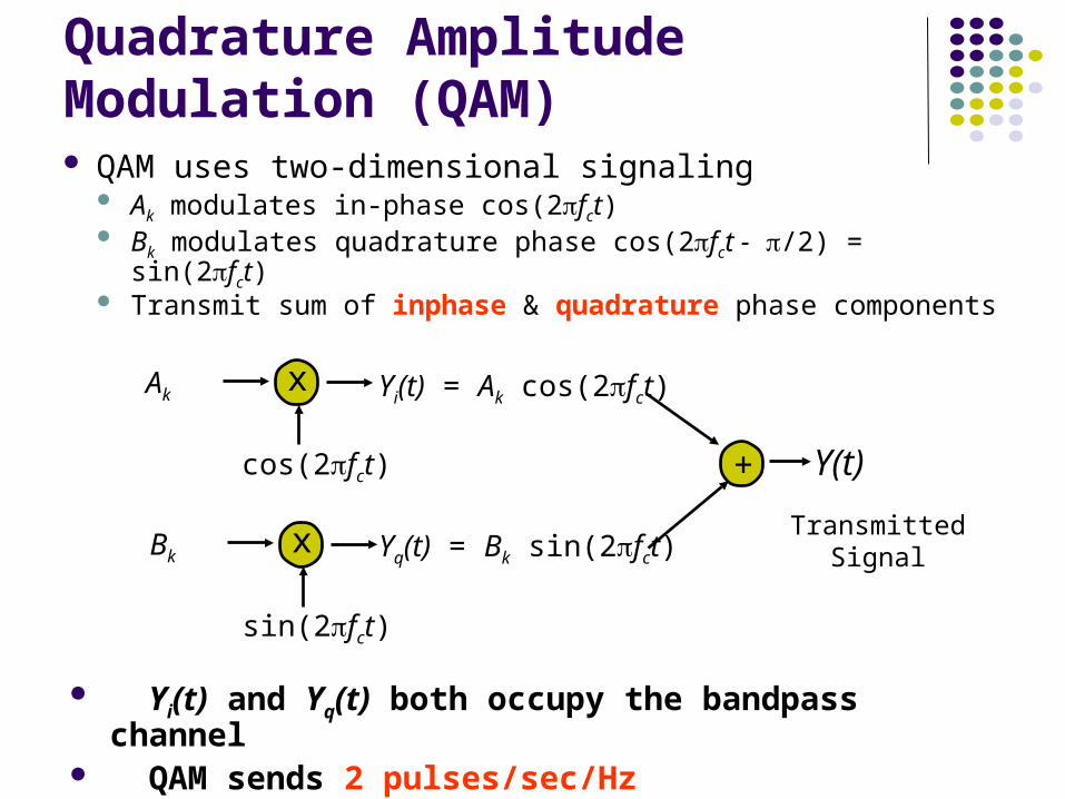
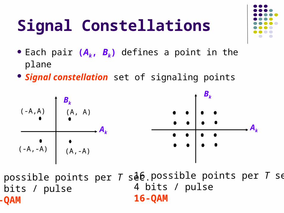
Akx

cos(2fct)

Yi(t) = Ak cos(2fct)

Bkx

sin(2fct)

Yq(t) = Bk sin(2fct)

+ Y(t)

Yi(t) and Yq(t) both occupy the bandpass channel QAM sends 2 pulses/sec/Hz

Quadrature Amplitude Modulation (QAM) QAM uses two-dimensional signaling

Ak modulates in-phase cos(2fct) Bk modulates quadrature phase cos(2fct - /2) = sin(2fct) Transmit sum of inphase & quadrature phase components

TransmittedSignal

QAM Demodulation

Y(t) x

2cos(2fct)2Akcos2(2fct)+2Bk cos(2fct)sin(2fct) = Ak {1 + cos(4fct)}+Bk {0 + sin(4fct)}

Lowpassfilter

(smoother)Ak

2Bk sin2(2fct)+2Ak cos(2fct)sin(2fct) = Bk {1 - cos(4fct)}+Ak {0 + sin(4fct)}

x

2sin(2fct)

Bk

Lowpassfilter

(smoother)

smoothed to zero

smoothed to zero

Signal Constellations

Each pair (Ak, Bk) defines a point in the plane Signal constellation set of signaling points

4 possible points per T sec.2 bits / pulse4-QAM

Ak

Bk

16 possible points per T sec.4 bits / pulse16-QAM

Ak

Bk

(A, A)

(A,-A)(-A,-A)

(-A,A)

Ak

Bk

4 possible points per T sec.

Ak

Bk

16 possible points per T sec.

Other Signal Constellations

Point selected by amplitude & phase

Ak cos(2fct) + Bk sin(2fct) = √Ak2 + Bk

2 cos(2fct + tan-1(Bk/Ak))

QPSK

Digital Transmission Fundamentals

Properties of Media and Digital Transmission Systems

Fundamental Issues in Transmission Media

Information bearing capacity Amplitude response & bandwidth Susceptibility to noise & interference

Propagation speed of signal c = 3 x 108 meters/second in vacuum = c/√speed of light in medium where is the

dielectric constant of the medium = 2.3 x 108 m/sec in copper wire; = 2.0 x 108 m/sec in

optical fiber

t = 0t = d/c

Communication channel

d meters

Communications systems & Electromagnetic Spectrum

Frequency of communications signals

Analog telephone

DSL Cell phone

WiFiOptical

fiber

102 104 106 108 1010 1012 1014 1016 1018 1020 1022 1024

Frequency (Hz)

Wavelength (meters)

106 104 102 10 10-2 10-4 10-6 10-8 10-10 10-12 10-14

Pow

er a

nd te

leph

one

Bro

adca

stra

dio

Mic

row

ave

radi

o

Infr

ared

ligh

t

Vis

ible

ligh

t

Ultr

avio

let l

ight

X-r

ays

Gam

ma

rays

Wireless & Wired Media

Wireless Media Signal energy propagates in

space, limited directionality Interference possible, so

spectrum regulated Limited bandwidth Simple infrastructure:

antennas & transmitters No physical connection

between network & user Users can move

Wired Media Signal energy contained &

guided within medium Spectrum can be re-used in

separate media (wires or cables), more scalable

Extremely high bandwidth Complex infrastructure:

ducts, conduits, poles

Attenuation

Attenuation varies with media Dependence on distance of central importance

Wired media Received power at d meters proportional to 10-kd Attenuation in dB ~ k d, where k is dB/meter.

Wireless media Received power at d meters proportional to d-n Attenuation in dB ~ n log10 d, where n is path loss

exponent; n=2 in free space; usually n is between 2 and 4. Signal level maintained for much longer distances Space communications possible

Twisted PairTwisted pair

Two insulated copper wires arranged in a regular spiral pattern to minimize interference

Various thicknesses, e.g. 0.016 inch (24 gauge)

Low cost Telephone subscriber loop

from customer to CO Old trunk plant connecting

telephone COs Intra-building telephone

from wiring closet to desktop

Att

enua

tion

(dB

/mi)

f (kHz)

19 gauge

22 gauge

24 gauge26 gauge

6

12

18

24

30

110 100 1000

Lower attenuation rate

analog telephone

Higher attenuation rate

for DSL

Twisted Pair Bit Rates Twisted pairs can provide

high bit rates at short distances

Asymmetric Digital Subscriber Loop (ADSL) High-speed Internet Access Lower 3 kHz for voice Upper band for data 64 kbps inbound 640 kbps outbound

Much higher rates possible at shorter distances Strategy for telephone

companies is to bring fiber close to home & then twisted pair

Higher-speed access + video

Data rates of 24-gauge twisted pair

Standard Data Rate Distance

T-1 1.544 Mbps 18,000 feet, 5.5 km

DS2 6.312 Mbps 12,000 feet, 3.7 km

1/4 STS-1 12.960 Mbps

4500 feet, 1.4 km

1/2 STS-1 25.920 Mbps

3000 feet, 0.9 km

STS-1 51.840 Mbps

1000 feet, 300 m

Coaxial Cable

Cylindrical braided outer conductor surrounds insulated inner wire conductor

High interference immunity Higher bandwidth than

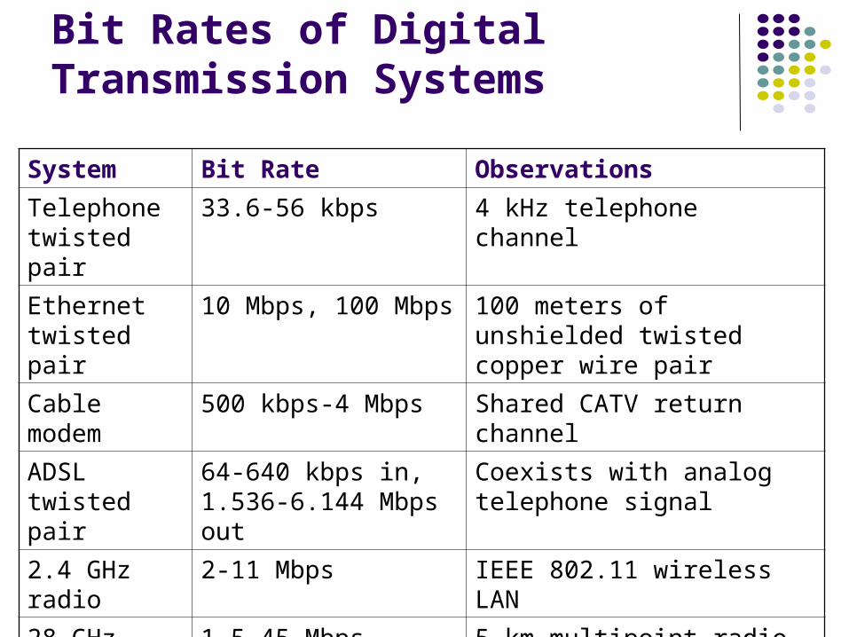
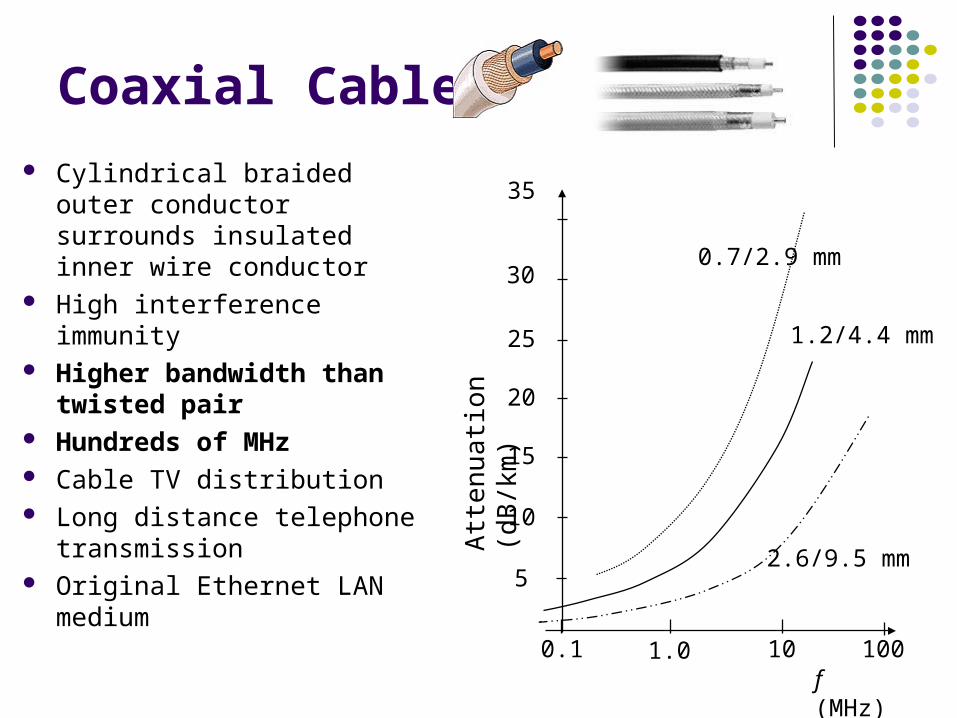
twisted pair Hundreds of MHz Cable TV distribution Long distance telephone

transmission Original Ethernet LAN

medium

35

30

10

25

20

5

15A

tten

uatio

n (

dB/k

m)

0.1 1.0 10 100f (MHz)

2.6/9.5 mm

1.2/4.4 mm

0.7/2.9 mm

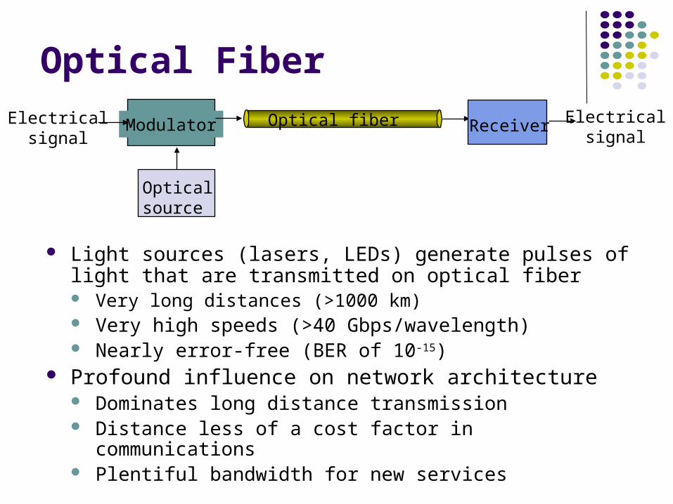
Optical Fiber

Light sources (lasers, LEDs) generate pulses of light that are transmitted on optical fiber Very long distances (>1000 km) Very high speeds (>40 Gbps/wavelength) Nearly error-free (BER of 10-15)

Profound influence on network architecture Dominates long distance transmission Distance less of a cost factor in communications Plentiful bandwidth for new services

Optical fiber

Opticalsource

ModulatorElectricalsignal

Receiver Electricalsignal

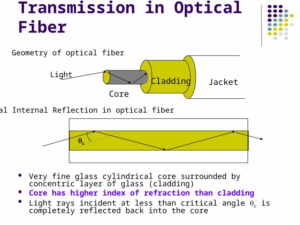
Core

Cladding JacketLight

c

Geometry of optical fiber

Total Internal Reflection in optical fiber

Transmission in Optical Fiber

Very fine glass cylindrical core surrounded by concentric layer of glass (cladding)

Core has higher index of refraction than cladding Light rays incident at less than critical angle c is completely reflected

back into the core

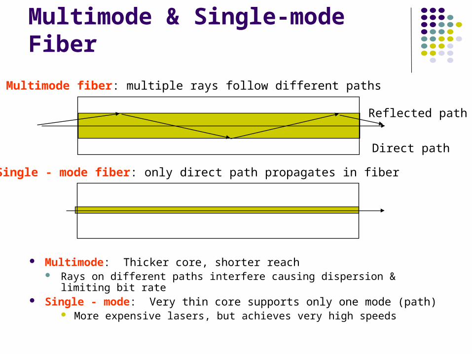
Multimode: Thicker core, shorter reach Rays on different paths interfere causing dispersion & limiting bit rate

Single - mode: Very thin core supports only one mode (path) More expensive lasers, but achieves very high speeds

Multimode fiber: multiple rays follow different paths

Single - mode fiber: only direct path propagates in fiber

Direct path

Reflected path

Multimode & Single-mode Fiber

100

50

10

5

1

0.5

0.1

0.05

0.010.8 1.0 1.2 1.4 1.6 1.8 Wavelength (m)

Loss

(dB

/km

)

Infrared absorption

Rayleigh scattering

Very Low Attenuation

850 nmLow-cost LEDs

LANs

1300 nmMetropolitan Area

Networks“Short Haul”

1550 nmLong Distance Networks

“Long Haul

Water Vapor Absorption(removed in new fiber

designs)

100

50

10

5

1

0.5

0.1

0.8 1.0 1.2 1.4 1.6 1.8

Loss

(dB

/km

)

Huge Available Bandwidth

Optical range from λ1to λ1Δλ contains bandwidth

Example: λ1= 1450 nm

λ1Δλ =1650 nm:

B = ≈ 19 THz

B = f1 – f2 = – v λ1 +

Δλ

v

λ1

v Δλ λ1

2= ≈ Δλ / λ1

1 + Δλ /

λ1

v

λ1

2(108)m/s 200nm (1450 nm)2

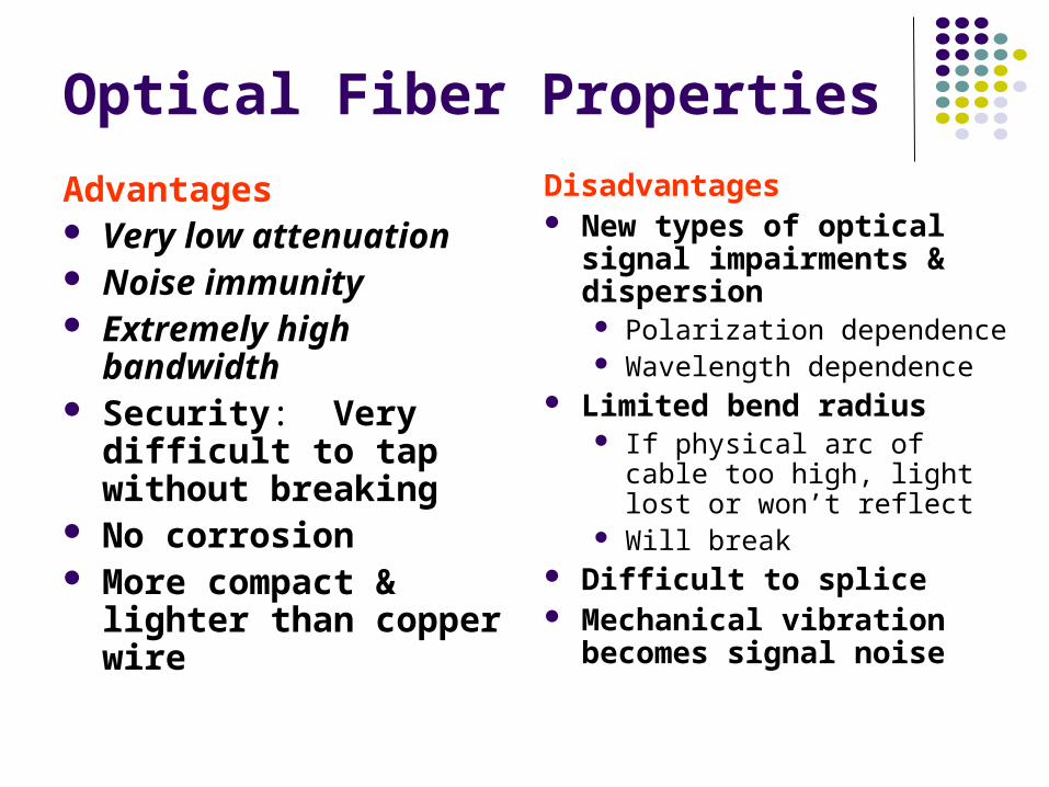
Optical Fiber Properties

Advantages Very low attenuation Noise immunity Extremely high

bandwidth Security: Very difficult

to tap without breaking No corrosion More compact & lighter

than copper wire

Disadvantages New types of optical signal

impairments & dispersion Polarization dependence Wavelength dependence

Limited bend radius If physical arc of cable too

high, light lost or won’t reflect Will break

Difficult to splice Mechanical vibration

becomes signal noise

Radio Transmission Radio signals: antenna transmits sinusoidal signal

(“carrier”) that radiates in air/space Information embedded in carrier signal using

modulation, e.g. QAM Communications without tethering

Cellular phones, satellite transmissions, Wireless LANs Multipath propagation causes fading Interference from other users Spectrum regulated by national & international

regulatory organizations (in general) There is also unlicensed spectrum (e.g., UNII

band).

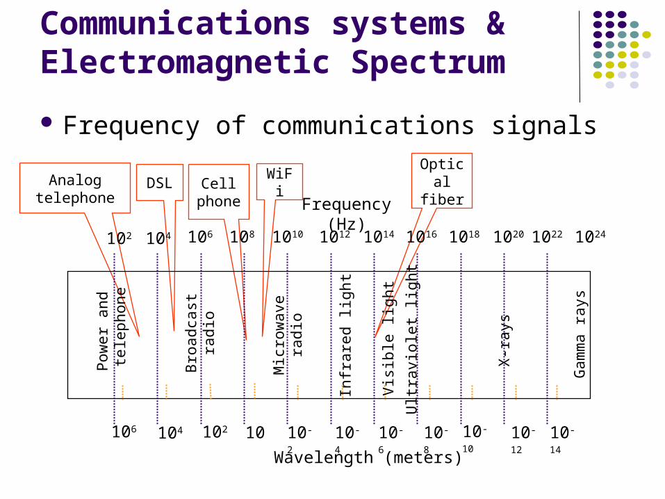
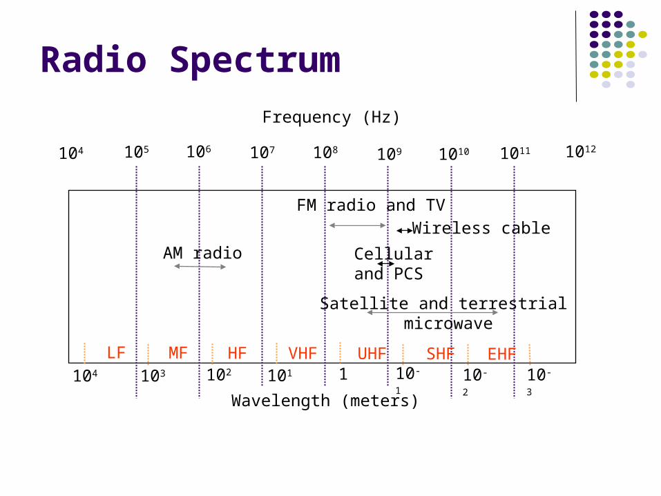
104 106 107 108 109 1010 1011 1012

Frequency (Hz)

Wavelength (meters)

103 102 101 1 10-1 10-2 10-3

105

Satellite and terrestrial microwave

AM radio

FM radio and TV

LF MF HF VHF UHF SHF EHF104

Cellularand PCS

Wireless cable

Radio Spectrum

ExamplesCellular Phone Allocated spectrum First generation:

800, 900 MHz Initially analog voice

Second generation: 1800-1900 MHz Digital voice, messaging

Wireless LAN Unlicenced ISM spectrum

Industrial, Scientific, Medical 902-928 MHz, 2.400-2.4835 GHz,

5.725-5.850 GHz IEEE 802.11 LAN standard

802.11a uses the 5 GHz Unlicensed National Information Infrastructure (U-NII) band

802.11b and 802.11g use the 2.4 GHz ISM band

Point-to-Multipoint Systems Directional antennas at

microwave frequencies High-speed digital

communications between sites High-speed Internet Access

Radio backbone links for rural areas

Satellite Communications Geostationary satellite @ 36000

km above equator Relays microwave signals from

uplink frequency to downlink frequency

Long distance telephone Satellite TV broadcast

Digital Transmission Fundamentals

Synchronization

Synchronous and Asynchronous Transmission

Synchronization Synchronization of

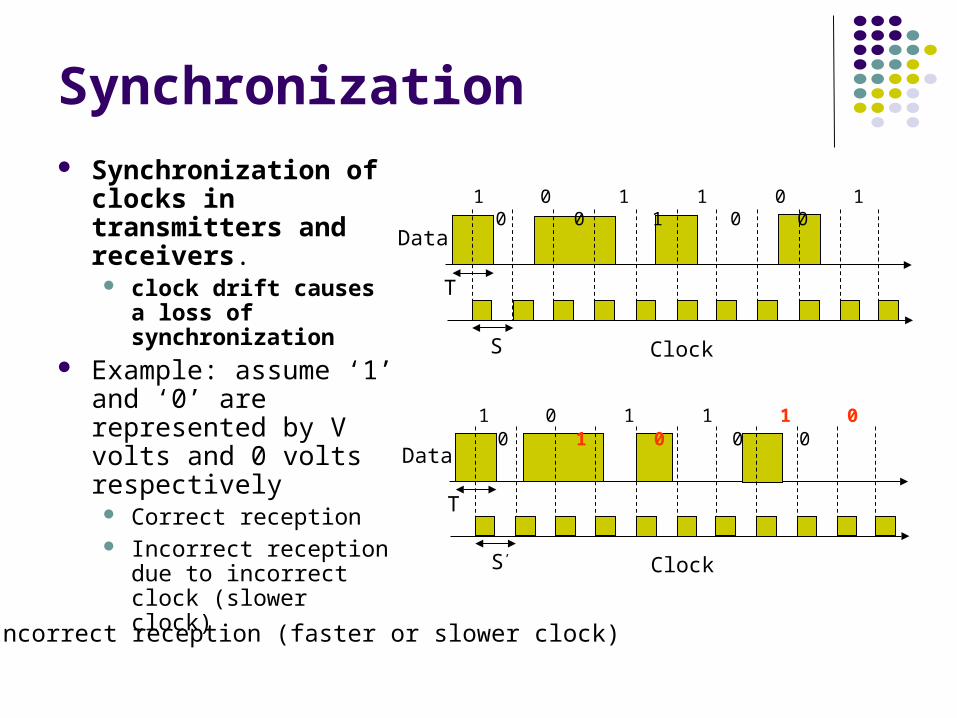
clocks in transmitters and receivers. clock drift causes a

loss of synchronization

Example: assume ‘1’ and ‘0’ are represented by V volts and 0 volts respectively Correct reception Incorrect reception due

to incorrect clock (slower clock)

Clock

Data

S

T

1 0 1 1 0 1 0 0 1 0 0

Clock

Data

S’

T

1 0 1 1 1 0 0 1 0 0 0

- Incorrect reception (faster or slower clock)

Synchronization (cont’d) How to avoid a loss of synchronization?

Synchronous transmission

Asynchronous transmission

Synchronous Transmission Sequence contains data + clock information (line coding)

i.e. Manchester encoding, self-synchronizing codes, is used.

PLL (phase-lock loop) is used to synch receiver clock to the transmitter’s clock

Asynchronous Transmission

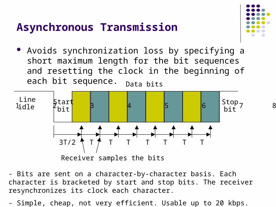
Avoids synchronization loss by specifying a short maximum length for the bit sequences and resetting the clock in the beginning of each bit sequence.

Startbit

Stopbit1 2 3 4 5 6 7 8

Data bits

Lineidle

3T/2 T T T T T T T

Receiver samples the bits

- Bits are sent on a character-by-character basis. Each character is bracketed by start and stop bits. The receiver resynchronizes its clock each character.

- Simple, cheap, not very efficient. Usable up to 20 kbps.