National Park Service U.S. Department of the Interior Natural Resource Program Center Digital Vegetation Maps for the NPS Cumberland- Piedmont I&M Network Final Report November 1, 2010 Natural Resource Technical Report NPS/CUPN/NRTR—2010/406
Transcript
National Park Service U.S. Department of the Interior Natural Resource Program Center
Perspective view of Carl Sandburg Home created from a USGS DEM and color orthophoto produced by the Center for Remote Sensing and Mapping Science, UGA. Produced by: John Dolesal
Thomas R. Jordan and Marguerite Madden Center for Remote Sensing and Mapping Science (CRMS) Department of Geography The University of Georgia Athens, Georgia, 30602-2503
November 2010
U.S. Department of the Interior National Park Service Natural Resource Program Center Fort Collins, Colorado
ii
The National Park Service, Natural Resource Program Center publishes a range of reports that address natural resource topics of interest and applicability to a broad audience in the National Park Service and others in natural resource management, including scientists, conservation and environmental constituencies, and the public.
The Natural Resource Technical Report Series is used to disseminate results of scientific studies in the physical, biological, and social sciences for both the advancement of science and the achievement of the National Park Service mission. The series provides contributors with a forum for displaying comprehensive data that are often deleted from journals because of page limitations.
All manuscripts in the series receive the appropriate level of peer review to ensure that the information is scientifically credible, technically accurate, appropriately written for the intended audience, and designed and published in a professional manner. This report received informal peer review by subject-matter experts who were not directly involved in the collection, analysis, or reporting of the data. This report received formal peer review by subject-matter experts who were not directly involved in the collection, analysis, or reporting of the data, and whose background and expertise put them on par technically and scientifically with the authors of the information
Views, statements, findings, conclusions, recommendations, and data in this report do not necessarily reflect views and policies of the National Park Service, U.S. Department of the Interior. Mention of trade names or commercial products does not constitute endorsement or recommendation for use by the U.S. Government.
This report is available from (http://www.crms.uga.edu/index.htm) and the Natural Resource Publications Management website (http://www.nature.nps.gov/publications/NRPM). (http://www.nature.nps.gov/publications/NRPM/).
Please cite this publication as:
Jordan, T.R., and M. Madden, 2010. Digital Vegetation Maps for the NPS Cumberland-Piedmont I&M Network: Final Report November 1, 2010. Natural Resource Technical Report NPS/CUPN/NRTR—2010/406. National Park Service, Fort Collins, Colorado.
NPS 910/106100, November 2010
iii
Contents
Page
Figures............................................................................................................................................ iv
Tables ............................................................................................................................................. vi
Summary ...................................................................................................................................... viii
Acknowledgments.......................................................................................................................... ix
Final Map Creation ................................................................................................................ 25
Summary and Conclusion ............................................................................................................. 27
Literature Cited ............................................................................................................................. 29
iv
Figures
Page
Figure 1: Location map for the Cumberland Piedmont (CUPN) I&M parks. ............................... 3
Figure 2: A portion of a color infrared aerial photograph of the Ninety Six NHS recorded in October 2002 and used for photo interpretation of vegetation detail. ............................................ 4
Figure 3: Diagram showing photogrammetric, photo interpretation and GIS operations used to map the vegetation of GRSM. .................................................................................................... 6
Figure 4: Well-defined natural and manmade features were used as pass points in overlapping images (yellow cross in circle symbols in the photos above). At least nine pass points per photo were identified with six being in the stereo overlap area between adjacent photos. ............................................................................................................................................. 9
Figure 5: The elevations of ground control points (GCPs) were determined from the 30-m digital elevation model (DEM) using a bilinear interpolation algorithm. .................................... 10
Figure 6: Nine pass points per photo and additional GCPs are measured and transferred to adjacent photos in the flight line. .................................................................................................. 11
Figure 7: A mosaic of orthorectified 1:12,000-scale photographs of Font Donelson was created for quality assurance and checking and to provide an image backdrop for the GIS database. ........................................................................................................................................ 11
Figure 8: Conducting a field survey of the vegetation at Ninety Six NHS prior to beginning detailed photo interpretation. During this field survey, the vegetation communities are explored to correlate the community with its appearance on the aerial photograph. ................... 14
Figure 9: Field map for Stones River National Battlefield used for field data collection with UTM grid, USGS DOQQ image, topographic contours, roads and rivers. .................................. 14
Figure 10: Ground digital image of overstory and understory vegetation recorded with a Kodak FIS 265 digital camera interfaced to a Garmin III Plus GPS. ........................................... 15
Figure 11: Sample CRMS Vegetation Classification System for Stones River National Battlefield that combines classes of the National Vegetation Classification System (NVCS), modified NVCS classes, landuses and special modifiers. ............................................................ 17
Figure 12: The CRMS Vegetation Classification System for Stones River National Battlefield includes modifications to the National Vegetation Classification System (NVCS) that indicate early successional (7124s) and managed (7124p) versions of CEGL associations (7124)........................................................................................................................ 18
Figure 13: The CRMS Vegetation Classification System for Stones River National Battlefield includes additional land cover classes that indicate management practices such as
v
planted savannah maintained by mowing (SAVpm) or land uses such as old or present home sites (HI)........................................................................................................................................ 18
Figure 15: (a) Original photo overlay depicting vegetation polygons and a 1-cm grid before corrections for relief displacement. (b) Overlay and grid after orthorectification showing the extreme corrections required to accommodate the large range of relief in the area. .................... 20
Figure 16: Full overlay that has been orthorectifed and is ready for raster-to-vector conversion. The uneven edges are a result of the differential rectification process that removes the relief displacements from the photos. ....................................................................... 21
Figure 17: Individual (unedited) vector files from four adjacent photos. .................................... 22
Figure 18: Section of the vegetation database that has been edited, edge matched and attributed. ...................................................................................................................................... 22
Figure 19: Final map product for Guilford Courthouse National Military Park (GUCO). ......... 26
vi
Tables
Page
Table 1: CUPN Parks, photo acquisition dates and scales and park sizes. .................................... 4
Table 2: Specifications of data sources available for map/database development of the Cumberland-Piedmont Network parks vegetation databases. ........................................................ 7
Table 3: Summary of vegetation mapping for CUPN parks. ....................................................... 24
vii
Appendices Page
Appendix A : Abraham Lincoln Birthplace National Historic Site and Abraham Lincoln Birthplace National Historic Site (Boyhood Home - Knob Creek Farm) .................................... 32
Appendix B: Carl Sandburg Home National Historic Site ........................................................... 42
Appendix C: Cowpens National Battlefield ................................................................................. 49
Appendix D: Cumberland Gap National Historical Park ............................................................. 56
Appendix E: Fort Donelson National Battlefield .......................................................................... 66
Appendix F: Guilford Courthouse National Military Park ........................................................... 73
Appendix G: Little River Canyon National Preserve ................................................................... 80
Appendix H: Ninety Six National Historic Site ............................................................................ 93
Appendix I: Stones River National Battlefield ........................................................................... 101
Appendix J: Chickamauga and Chattanooga National Military Park, Lookout Mountain Battlefield, and Moccasin Bend .................................................................................................. 110
Appendix K: Kings Mountain National Military Park .............................................................. 129
Appendix L: Mammoth Cave National Park .............................................................................. 137
Appendix M: Russell Cave National Monument ........................................................................ 147
Appendix N: Shiloh National Military Park ............................................................................... 154
viii
Summary
This report describes the vegetation mapping procedures employed by the Center for Remote Sensing and Mapping Science (CRMS), Department of Geography, University of Georgia, This report describes the procedures and results of the vegetation mapping activities undertaken by the CRMS under Cooperative Agreements No. H5028 01 0651, entitled, ―Digital Vegetation
Databases and Maps for National Park Service Units in the Appalachian Highlands and Cumberland/Piedmont Networks‖ and No. H 5000-03-5040, Task No. J2-113-05-5004, entitled ―Vegetation Databases, Orthoimages and Buffer-Area Land Cover in Four National Park Units of the Cumberland/Piedmont Network.‖ The fourteen parks included in this report range in size from 50 to 20392 hectares (122 to 50390 acres) and include Abraham Lincoln NHS, Carl Sandburg Home NHS, Cowpens NB, Cumberland Gap NHP, Fort Donelson NB, Guilford Courthouse NMP, Little River Canyon NPRES, Ninety Six NHS, Stones River NB, Chickamauga and Chattanooga NMP, Kings Mountain NMP, Mammoth Cave NP, Russell Cave NM, and Shiloh NMP.
Using the National Vegetation Classification System (NVCS) developed by Natureserve, with additional classes and modifiers, overstory vegetation communities for each park were interpreted from stereo color infrared aerial photographs using manual interpretation methods. Using a minimum mapping unit of 0.5 hectares (MMU = 0.5 ha), polygons representing areas of relatively uniform vegetation were delineated and annotated on clear plastic overlays registered to the aerial photographs. Polygons were labeled according to the dominant vegetation community. Where the polygons were not uniform, second and third vegetation classes were added. Further, a number of modifier codes were employed to indicate important aspects of the polygon that could be interpreted from the photograph (for example, burn condition).
The polygons on the plastic overlays were then corrected using photogrammetric procedures and converted to vector format for use in creating a geographic information system (GIS) database for each park. In addition, high resolution color orthophotographs were created from the original aerial photographs for use in the GIS. Upon completion of the GIS database (including vegetation, orthophotos and updated roads and hydrology layers), both hardcopy and softcopy maps were produced for delivery.
Metadata for each database includes a description of the vegetation classification system used for each park, summary statistics and documentation of the sources, procedures and spatial accuracies of the data. At the time of this writing, an accuracy assessment of the vegetation mapping has not been performed for most of these parks. Thus, those procedures and results are not included in this report.
This report describes the procedures and results of the vegetation mapping activities undertaken by the CRMS under Cooperative Agreements No. H5028 01 0651, entitled, ―Digital Vegetation
Databases and Maps for National Park Service Units in the Appalachian Highlands and Cumberland/Piedmont Networks‖ and No. H 5000-03-5040, Task No. J2-113-05-5004, entitled ―Vegetation Databases, Orthoimages and Buffer-Area Land Cover in Four National Park Units of the Cumberland/Piedmont Network.‖
ix
Acknowledgments
This study was sponsored by the U.S. Department of Interior, National Park Service, (Cooperative Agreements No. H5000 03 5040 and H 5000-03-5040). The authors wish to express their appreciation for the devoted efforts of the staff at the Center for Remote Sensing and Mapping Science, The University of Georgia, the NPS Cumberland-Piedmont Network and NatureServe. Individuals from the above mentioned organizations, as well as others who have participated in this project include: Ben Downey, John Dolezal, Adam Hinely, Amanda Humpries, Tom Govas, Phyllis Jackson, Charles Jordan, Teresa Leibfried, Louis Manglass, Janna Masour, Jennifer Pierce, Tyler Plain, Mylo Pyne, Heather Russell, Lillian Scoggins, Jean Seavey, Rick Seavey, Chris Watson, Roy Welch, Rickie White and Mark Whited.
Digital Vegetation Maps for the CUPN Network
Digital Vegetation Maps for the CUPN Network
1
Introduction:
As part of the USGS/BRD-NPS Vegetation Mapping Program, the Center for Remote Sensing and Mapping Science (CRMS), Department of Geography, University of Georgia, was requested to provide detailed vegetation maps of a number of national park units in the Cumberland Piedmont Inventory and Monitoring Network (CUPN) of the National Park Service. This report describes the procedures and results of the vegetation mapping activities undertaken by the CRMS under Cooperative Agreements No. H5028 01 0651, entitled, ―Digital Vegetation Databases and Maps for National Park Service Units in the
Appalachian Highlands and Cumberland/Piedmont Networks‖ and No. H 5000-03-5040, Task No. J2-113-05-5004, entitled ―Vegetation Databases, Orthoimages and Buffer-Area Land Cover in Four National Park Units of the Cumberland/Piedmont Network.‖
The fourteen parks included in this report range in size from 50 to 20392 hectares (122 to 51341 acres) and include Abraham Lincoln NHS, Carl Sandburg Home NHS, Cowpens NB, Cumberland Gap NHP, Fort Donelson NB, Guilford Courthouse NMP, Little River Canyon NPRES, Ninety Six NHS, Stones River NB, Chickamauga and Chattanooga NMP, Kings Mountain NMP, Mammoth Cave NP, Russell Cave NM, and Shiloh NMP. Using the National Vegetation Classification System (NVCS) developed by Natureserve, with additional classes and modifiers, overstory vegetation communities for each park were interpreted from large-scale stereo color infrared aerial photographs using manual interpretation methods. Using a minimum mapping unit of 0.5 hectares (MMU = 0.5 ha), polygons representing areas of relatively uniform vegetation were delineated and annotated on clear plastic overlays registered to the aerial photographs. Polygons were labeled with CEGL codes according to the dominant vegetation community. Where the polygons were not uniform, second and third vegetation classes were added. Further, a number of modifier codes were employed to indicate important aspects of the polygon that could be interpreted from the photograph (for example, burn condition).
The polygons on the plastic overlays were then corrected using photogrammetric procedures and converted to vector format for use in creating a geographic information system (GIS) database for each park. In addition, high resolution color orthophotographs were created from the original aerial photographs for use in the GIS. Upon completion of the GIS database (including vegetation, orthophotos and updated roads and hydrology layers), both hardcopy and softcopy maps were produced for delivery.
Metadata for each database includes a description of the vegetation classification system used for each park, summary statistics and documentation of the sources, procedures and spatial accuracies of the data. At the time of this writing, an accuracy assessment of the vegetation mapping has not been performed for most of these parks. Thus, those procedures and results are not included in this report.
The Center for Remote Sensing and Mapping Science (CRMS), Department of Geography at The University of Georgia, (www.crms.uga.edu) has been involved in vegetation mapping and database development in national parks of the southeastern U.S. for the past 10 years (Welch et al. 1995, 1999, 2002a, 2002b; Welch and Remillard 1996). As a remote sensing and mapping facility, the CRMS is unique in is combination of expertise in
both technical and biological aspects of vegetation mapping projects. Scientists at the CRMS specialize in image processing, photogrammetry, GIS, air photo interpretation and field surveying, as well as botany, biology and ecology. This allows a close link between the two major components of a vegetation mapping/database project: 1) photogrammetric rectification and GIS database construction; and 2) vegetation interpretation, classification and field verification.
In addition to in-house cross training of technical and biological skills, the CRMS has developed a strong working relationship with NatureServe, a non-profit conservation organization that developed the U.S. National Vegetation Classification System (NVCS) and is a primary partner in the USGS-NPS Vegetation Mapping Program (www.natureserve.org). Collaboration between the CRMS and the NatureServe-Durham, North Carolina Office has resulted in the development of a detailed classification system for southeastern park lands that maximizes the information on vegetation communities that can be gleaned from large-scale color infrared aerial photographs, while remaining compatible with the U.S. National Vegetation Classification System (Anderson et al. 1998, Jackson et al. 2002).
Objectives
The objectives of this report are to:
1. describe the mapping procedures employed to map the vegetation communities of the parks in the NPS Cumberland Piedmont I&M Network (CUPN) ;
2. demonstrate how digital photogrammetry, photointerpretation, GIS and Global Positioning Systems (GPS)-assisted field techniques were refined, adapted and integrated to permit the construction of geocoded vegetation databases from large-scale aerial photographs;
3. discuss the NVCS in general and its adaptation for use in the Cumberland Piedmont parks; and
4. provide classification systems, summary statistics and vegetation maps for each park.
Digital data in the form of ArcGIS geodatabases, shapefiles, orthophotos and metadata are provided on the accompanying DVDs. Most of the techniques described below were first developed and refined during the mapping of Great Smoky Mountains National Park, which is considered to be one of the most difficult terrain areas to map in the United States (Jordan, 2002; Welch et al., 2004).
Study Area
The Cumberland-Piedmont Network (CUPN) encompasses 14 national parks with diverse cultural and natural resources distributed across seven states and six different physiographic regions in the southeastern United States. This report summarizes the
vegetation mapping work for those parks which include historic sites, battlefields, military parks and recreation areas in North Carolina, South Carolina, Alabama, Tennessee and Kentucky. The following parks are included in this report: Abraham Lincoln NHS (ABLI), Carl Sandburg Home NHS (CARL), Cowpens NB (COWP), Cumberland Gap NHP (CUGA), Fort Donelson NB (FODO), Guilford Courthouse NMP (GUCO), Little River Canyon NPRES (LIRI), Ninety Six NHS (NISI), Stones River NB (STRI), Chickamauga and Chattanooga NMP (CHCH), Kings Mountain NMP (KIMO), Mammoth Cave NP (MACA), Russell Cave NM (RUCA), and Shiloh NMP (SHIL) (Figure 1).
Figure 1: Location map for the Cumberland Piedmont (CUPN) I&M parks.
Requirements
The primary requirement for the project was to produce a vegetation database and associated maps in vector format that contained polygons for overstory plant communities plotted to within approximately +5 to 10 m of their true ground locations. Overstory vegetation was mapped using color infrared aerial photographs of 1:12,000 and 1:16,000 scale in film transparency format recorded with a standard photogrammetric mapping camera (f = 15 cm) in late October and early-November by the U. S. Forest Service and Air Photographics (Martinsville, WV). The fall photos were acquired when the leaves were still on the trees (leaf-on) and displayed a color diversity that allowed the vegetation communities/species to be identified (Table 1, Figure 2). Relief displacements were a major consideration in the mountainous areas and required photogrammetric correction methods in order to ensure geometric accuracy (Jordan, 2004). Using ground control obtained from USGS Digital Orthophoto Quarter-Quads (DOQQ) and the National
Digital Vegetation Maps for the CUPN Network
4
Elevation Dataset (NED), polygons were plotted to within approximately + 5 m of their true ground locations, thus meeting National Map Accuracy Standards for 1:15,000 scale maps.
Table 1: CUPN Parks, photo acquisition dates and scales and park sizes.
PARK Park Name Photo date(s) photo scale Area (ac)
CHCH Chickamauga and Chattanooga NMP; Lookout Mountain; Moccasin Bend and Reservations 10/30/2001 1:12,000 5,534; 3,353; 70
KIMO Kings Mountain NMP 10/24/2000 1:12,000 3,955 MACA Mammoth Cave NP 11/08/2001 1:16,000 51,341 RUCA Russell Cave NM 10/25/2001 1:12,000 317 SHIL Shiloh NMP 10/25/2001 1:12,000 3,960 CARL Carl Sandburg Home NHS 10/24/00; 11/2/02 1:12,000 260 GUCO Guilford Courthouse NMP 10/20/2000 1:12,000 203 CUGA Cumberland Gap NHP 11/2/2002 1:16,000 20061 LIRI Little River Canyon NPRES 10/31/2001 1:12,000 13698 NISI Ninety Six NHS 10/24/2000 1:12,000 948 STRI Stones River NB 10/25/2001 1:12,000 654 ABLI Abraham Lincoln NHS (Boyhood Home ) 11/2/2002 1:12,000 264 ABLI Abraham Lincoln NHS (Birthplace) 11/2/2002 1:12,000 122 COWP Cowpens NB 11/2/2002 1:12,000 839 FODO Fort Donelson NB 11/2/2002 1:12,000 518
Figure 2: A portion of a color infrared aerial photograph of the Ninety Six NHS recorded in October 2002 and used for photo interpretation of vegetation detail.
Digital Vegetation Maps for the CUPN Network
5
In general, the mapping tasks are divided into four major categories of operations:
1. Collection and integration of collateral datasets;
2. Photogrammetry, which includes the initial scanning and orthorectifying of the CIR photographs and subsequent rectification of the interpreted overlays;
3. Photointerpretation and ground truthing, which includes delineation and attribution of polygons representing vegetation classes on aerial photographs; and
4. Geographic information systems (GIS), which includes converting the photointerpretation to vectors, editing and attributing the vegetation polygons and creating the final GIS database and hardcopy maps.
Final products include the following: 1. Overstory vegetation maps in digital format attributed according to the National
Vegetation Classification System (NVCS);
2. Generalized vegetation classes for a buffer area extending 400 m outside of the park boundary;
3. Digital orthophotos created from the CIR aerial photographs;
4. Updated roads and hydrology line work within park boundaries;
5. Hard and softcopy maps of the final databases; and
6. Metadata for the vegetation maps.
As most national parks are located in natural areas with typically dense forest cover, steep slopes, absence of ground control and high relief, the construction of a vegetation database accurate in both the spatial and thematic context necessitated a combination of softcopy photogrammetry, manual photo interpretation and GIS procedures organized in parallel as shown in Figure 3. These are discussed below.
Collateral Datasets
A base GIS dataset was compiled for each park that consisted of a combination of publicly available data layers (http://seamless.usgs.gov) and those provided by the park resource managers. Basic layers included existing roads and trails, hydrology, boundaries, digital raster graphics (DRGs), digital orthophoto quarter quads (DOQQs), digital elevation models (DEMs), and any available additional ancillary data layers, such as geology, soils, and historical vegetation maps. All data layers were cast on the Universal Transverse Mercator (UTM) coordinate system, North American Datum of 1983 (NAD83), in the UTM majority zone for the park location (Table 2).
Digital Vegetation Maps for the CUPN Network
6
Register Overlays to Photos
Measure fiducual mark coordinates on overlays.
Transfer passpoints from aerial photos to overlays
using affine transformation.
Orthocorrect Scanned Overlays
Compute exterior orientation parameters and create
orthoimages of overlays using USGS DEMs.
Raster to Vector Conversion
Convert corrected raster polygons
to Arc/Info vectors.
Integrate Corrected Vectors
to Create GIS Coverages
Merge coverages from all overlays.
Edit, edge-match and assign attributes.
Create Final GIS Database and Map Products
Add titles and perform final check of maps.
Scan Photos
Scan 1:12,000 or 1:16,000 CIR photos at
42 um (600 dpi) resolution.
Pass Points
Locate and measure photo coordinates (xy) of
fiducial marks and pass points on scanned photos.
Ground Control Points
Identify and digitize (XY) GCPs from USGS DOQQs.
Interpolate elevations (Z) of GCPs from
USGS Level 2 DEMs.
Aerotriangulation
Determine ground coordinates for pass points.
Photogrammetric
Operations
Prepare Photos for Interpretation
Register clear overlays to CIR photos. Annotate and
number fiducial marks.
Photointerpretation
Delineate vegetation polygons on the overlays.
Scan Overlays
Scan the full frames, including the annotated
fiducial marks. Digitize the fiducial marks.
Photointerpretation
Operations
Figure 3: Diagram showing photogrammetric, photo interpretation and GIS operations used to map the vegetation of GRSM.
Digital Vegetation Maps for the CUPN Network
7
Table 2: Specifications of data sources available for map/database development of the Cumberland-Piedmont Network parks vegetation databases.
Data Source Format and Type of Data
Flying Height (FH) and/or Scale
Resolution Comments
Color infrared (CIR) Air Photos October/ November 2002
23 x 23 cm Analog film transparencies
FH =1800 m 1:12,000 FH = 2400 m 1:16,000
~ 0.4 m 0.67 m
Fall leaf-on conditions are ideal for mapping overstory forest communities.
USGS Digital Raster Graphics Topographic Maps
Digital scanned topo maps
1:24,000 2.33 m Last updated 1970’s. A good base map but missing some more recent cultural features.
USGS DOQQs Pan (1993) and CIR (1999)
Digital Orthophotos
FH = 6000 m 1:40,000
1 m USGS DOQQs have a planimetric accuracy of approximately ± 3 m RMS. Winter photographs.
USGS Level 2 DEMs Digital Elevation Models
1:24,000 30 m post spacing
USGS Level 2 DEMs have a vertical accuracy of approximately ± 3-5 m RMS.
USGS DLG Census TIGER Line Files National Hydrology Dataset (NHD)
Digital vector data (shape files) roads, trails, hydrology, boundaries
1:24,000 N/A We used the best vector datasets available. Usually provided by the parks or retrieved from the USGS Seamless database.
Digital Vegetation Maps for the CUPN Network
8
Photogrammetric Operations
The main objective of the photogrammetric procedure was to create a set of color infrared orthophotos from the same aerial photographs that were being used for the vegetation mapping. To accomplish this, we first had to densify the sparse ground control in the Park by means of aerotriangulation, a photogrammetric operation whereby a relatively small number of ground control points (GCPs) are used to mathematically compute the ground coordinates of a much larger number of identified pass points (Jordan, 2002). In this way, an adequate control network is generated for the orthophoto rectification process. These control points were also used to rectify the interpretation overlays.
Scanning The CIR aerial photographs in transparency format were scanned at 600 dpi (42 µm) using an Epson Expression 10000XL flatbed scanner. This scanner is capable of scanning materials up to 11x17‖ in size at optical resolutions up to 1200 dpi and is equipped with a backlight attachment for scanning transparent materials. The 600 dpi scanning resolution was selected to balance the resolution requirements for the orthophotos with data storage and processing considerations. The photographs were laid on the scanning surface and, to reduce distortions, a heavy piece of clear glass was placed on top to ensure flatness of the film during scanning. Each photo was then scanned using Adobe Photoshop and saved as a 24-bit color TIFF file. During scanning, care was taken to scan the full frame of the photograph, including the corner fiducial marks and marginal data. File names for the scanned photographs were assigned according to the flight line and frame number. For example, photo 13 from flight line 2 was named 2-13.tif. Photos from each park were stored in separate folders on the CRMS Data server. All photos from each flight line were scanned. For original photos of 1:12,000 and 1:16,000 scales, the resulting pixel sizes were approximately 0.5 m and 0.67 m, respectively. After the photos were scanned, the original film transparencies were turned over to the photointerpreters while the photogrammetric operations continued using the digital data.
Ground Control and Pass Point Measurement These digital photos were then displayed on the computer monitor and with the aid of the R-WEL, Inc. Desktop Mapping System (DMS) software package, the image (x,y) coordinates of pass points and GCPs were measured in the softcopy (computer, heads-up digitizing) environment. This was a painstaking and time-consuming task. Pass points per photo were selected and measured on adjacent photographs. In some parks, there were enough cultural features so that features such as driveways, road intersections, parking lots, or sidewalks could be used as pass points. In other cases, it was necessary to use hay bales, bare spots in a field, creeks, rocks or trees as pass points (Figure 4).
Digital Vegetation Maps for the CUPN Network
9
Figure 4: Well-defined natural and manmade features were used as pass points in overlapping images (yellow cross in circle symbols in the photos above). At least nine pass points per photo were identified with six being in the stereo overlap area between adjacent photos.
Ground control points were, for the most part, well-defined man-made and natural features (e.g., road intersections, parking lots, rock outcrops and forks in stream channels) identified on both the scanned color infrared transparencies and USGS Digital Orthophoto Quarter Quads (DOQQs) produced from 1:40,000-scale panchromatic or color infrared (CIR) aerial photographs recorded in 1993 or 1998. The Universal Transverse Mercator (UTM) grid coordinates (X,Y tied to the North American Datum of 1983 or NAD 83) of these GCPs were measured directly from the DOQQs (accurate to within + 3 m). Elevations for the GCPs were derived using CRMS custom software to interpolate the Z-coordinates to within + 3 to + 5 m from USGS Level 2 Digital Elevation Models (DEMs) with 30-m post spacing (Figure 5). Thus, in this project, no ground survey work was required (or performed) to obtain the GCPs needed as a framework for the aerotriangulation process.
Digital Vegetation Maps for the CUPN Network
10
Figure 5: The elevations of ground control points (GCPs) were determined from the 30-m digital elevation model (DEM) using a bilinear interpolation algorithm.
Aerotriangulation Analytical aerotriangulation was undertaken on a flight line by flight line basis and then all of the flightlines for a park were merged for the final run. The Aerosys software package, in conjunction with the DMS software, was employed for the aerotriangulation process. Output from the aerotriangulation was a set of X, Y and Z coordinates in the UTM coordinate system for the nine or more pass points identified by CRMS personnel on each photo. Typical root-mean-square error (RMSE) values for these coordinates averaged + 5 m for the XY vectors and + 6 m for elevations (Z).
Nine pass points per are measured and transferred to adjacent photos in the flight line. In addition, a number of ground control points are measured on the DOQQ and each photo (Figure 6). In the aerotriangulation process, the individual photos are joined numerically, related to the ground coordinate system using the GCPs and then the ground coordinates of the pass points are calculated. This dense network of GCPs can then be used to orient and orthorectify the CIR aerial photographs and to generate orthophotomosaics (Figure 7). After the orthophotomosaic is generated, the seamlines between adjacent photos are examined for misalignment. Terrain features that are well aligned between individual photographs indicate a good overall solution. The orthophotos and mosaics, in turn, are employed as a base reference layer in the editing and attributing operations required to build the vector database.
A critical use of the aerotriangulated GCPs is in the rectification of the vector overlays generated as part of the photointerpretation procedure described below. A well-aligned orthophoto mosaic provides the geometry and foundation necessary for the rectified vegetation linework of individual photographs to be edgematched correctly during the editing process.
Digital Vegetation Maps for the CUPN Network
11
Pass Point
Control Point
Figure 6: Nine pass points per photo and additional GCPs are measured and transferred to adjacent photos in the flight line.
Figure 7: A mosaic of orthorectified 1:12,000-scale photographs of Font Donelson was created for quality assurance and checking and to provide an image backdrop for the GIS database.
Digital Vegetation Maps for the CUPN Network
12
Photointerpretation and Ground Truthing Operations
The steps of the photointerpretation process listed in Figure 3 proceeded in parallel with the photogrammetric operations. Overstory vegetation was interpreted from the 1:12,000 to 1:16,000 scale leaf-on color infrared aerial photographs in 9 x 9 inch film transparency format.
Although it might appear desirable to scan the color infrared transparencies at high resolution and undertake the vegetation classification as an on-screen interpretation and digitizing procedure, this has proved to be exceedingly time consuming, cumbersome and expensive compared to more traditional approaches (Welch et al. 1995 and 1999; Rutchey and Vilchek 1999). More importantly, photointerpreters must view the vegetation and the terrain in stereo and in color within the context of a relatively large area of the landscape in order to identify the vegetation communities. This is most easily done using a stereoscope to view the analog air photos so that the vegetation patterns can be assessed in relation to the terrain. Recognizing the need to augment manual procedures with automated techniques, the steps described below integrate conventional photointerpretation procedures with digital processing technology in an attempt to streamline the database and map compilation process.
At the beginning of each individual park‘s mapping project, the photointerpreters, in
conjunction with NatureServe and NPS plant specialists and resource managers, conducted field investigations to collect data on the vegetation communities and correlate signatures evident on the aerial photographs with ground observations. Photointerpreters learned about management concerns and impacts to the vegetation communities and their distributions such as damage by exotic insects, fire, wind, excessive park use, etc. Information on land use history before and after the creation of the park and invasive plant species also was critical to understanding past, present and future vegetation conditions.
The vegetation in some parks, especially the small battlefields, is highly managed to maintain the landscape and landuse/land cover of the time period for which the park was designated. All of these factors must be taken into consideration during the photointerpretation process to ensure a meaningful vegetation classification system is used for each park and to accurately identify and portray the vegetation communities. Depending on the size of the park, an initial reconnaissance field visit would be conducted for 2 to 5 days and include visits to representative habitats, rare and important communities and managed, disturbed or invaded areas, as well as revisits to plots previously surveyed by NatureServe. Additional field visits were conducted during the interpretation process to verify initial interpretations, identify communities with unusual signatures and answer any questions. A final field visit was usually conducted after the interpretation was complete and the vegetation database/maps were produced as a quality control check before the more rigorous accuracy assessments by NPS and NatureServe.
Field sampling consisted of field data collection at numerous points along and off trails within the parks that were representative of both typical vegetation communities and unique or highly damaged areas (Figure 8). . Methods and information collected resembled NatureServe‘s ―Quick Plot‖ surveys For an area approximately 15 to 20 m
Digital Vegetation Maps for the CUPN Network
13
around each point, the percent cover of dominant overstory and understory species was recorded, along with any additional overstory/understory species identified and characteristics of the herb layer such as rich, sparse, dominant species, etc. Site conditions were noted by recording relative slope, aspect and canopy openness. Notes on presence of exotics, evidence of past or present human influence (e.g., agriculture, grazing, logging, mowing, exotic vegetation removal, old homesites), damage by insects, wild hogs, blow down or fire also were recorded. Each point was geolocated by marking a waypoint with a Global Positioning System (GPS) handheld receiver such as a Garmin V or Garmin Geko. These units are Wide Area Augmentation System (WAAS)-enabled and typical horizontal positional accuracies were +/- 3 to 5 m. The Estimated Positional Error (EPE) was noted for each field waypoint collected, especially when error approached or exceeded +/- 10 m. The elevation of each field waypoint also was recorded, albeit vertical accuracy is generally more than two times lower than horizontal accuracy. As a back-up to the use of GPS for geolocation, field crews also carried paper field maps with the UTM grid coordinates, elevations, roads and rivers superimposed on an image background, usually a USGS DOQQ (Figure 9). The maps were useful in planning the field route, marking notes and augmenting the GPS digital display.
At each field point, the primary association type was determined based on NatureServe definitions of associations in the National Vegetation Classification System (NVCS) used in the USGS/NPS National Vegetation Mapping Program (i.e., NVCS Community Element Global (CEGL) code numbers) (Anderson et al. 1998, Grossman et al. 1998 and 1994). Since CRMS interpreters were usually accompanied by NatureServe botanists to assist with species identification and coordinate classification, interpretation and accuracy assessment efforts, CRMS and NatureServe personnel would discuss and agree on the association designation before moving on. If the field point was located in a mixed area indicative of an ecotone or an area of successional recovery, both the dominant and secondary (and sometimes tertiary) associations also were determined. If there was no good match to an NVCS CEGL, careful notes were taken to allow later assignment of the appropriate CEGL or CRMS-created class (e.g., a managed, damaged, human influence or successional class).
Digital Vegetation Maps for the CUPN Network
14
Figure 8: Conducting a field survey of the vegetation at Ninety Six NHS prior to beginning detailed photo interpretation. During this field survey, the vegetation communities are explored to correlate the community with its appearance on the aerial photograph.
Figure 9: Field map for Stones River National Battlefield used for field data collection with UTM grid, USGS DOQQ image, topographic contours, roads and rivers.
NatureServe had completed their field plot surveys and developed a classification field key for a particular park before CRMS-NatureServe field work was conducted, then the key would be jointly used, informally tested and modified. Although this process tended to
Digital Vegetation Maps for the CUPN Network
15
require considerable time that was outside of the scope of CRMS mapping tasks, its importance was recognized after NatureServe conducted some of the first accuracy assessments of CRMS vegetation databases. It is imperative that NVCS classes in the NatureServe field key match the classes used by CRMS for interpretation, definitions of the classes are not modified after the interpretation is completed and CRMS and NatureServe botanists agree on the classes the keys ―key-out‖ to.
During a full field day, the UTM coordinates and field data were typically collected at approximately 25 to 35 locations. Digital camera images were taken at most field points to document the vegetation and site conditions. In some parks, ground photos were tied to geographic locations with the aid of a Garmin III Plus hand-held GPS receiver and a Kodak Digital Field Imaging System (FIS) 265 digital camera system. The hand-held Kodak digital camera was connected to the Garmin GPS that ―stamped‖ the location, date
and time on each image (Figure 10). These images were input to ArcView to provide a pictorial record of field observations.
Figure 10: Ground digital image of overstory and understory vegetation recorded with a Kodak FIS 265 digital camera interfaced to a Garmin III Plus GPS.
A compilation of all field information was used by CRMS photointerpreters to connect the NVCS association-level classes identified in the field with photo signatures for vegetation patches identified on the color infrared aerial photographs. The locations of CRMS field points were transferred from the GPS units to ArcMap and superimposed on orthorectified images of each park. Information from the field points on overstory, understory and herbaceous strata, environmental site conditions and any notes on human influence or disturbance were used to delineate areas of homogeneous vegetation communities into areas (i.e., vegetation polygons) and label (i.e., attribute) polygons with the appropriate NVCS association class (i.e., CEGL).
Digital Vegetation Maps for the CUPN Network
16
The term, association, is defined by Grossman et al. (1998) as a ―plant community type of
definite floristic composition, uniform habitat conditions and uniform physiognomy‖.
Vegetation classification studies by NatureServe were conducted prior to CRMS photointerpretation in most parks to create a list of typical NVCS associations and provide a comprehensive description of species found in one to several strata of vegetation: tree canopy, sub-canopy, tall shrub, short shrub, herbaceous, non-vascular, vine/liana and epiphyte. The combination of vegetation in all of these strata present determines the community type and NVCS association CEGL. Additional information on global and local site conditions also are included in NatureServe park classification descriptions. This information was extremely helpful to CRMS interpreters and photointerpretation proceeded most smoothly when classification studies by NatureServe were completed prior to photointerpretation. Close cooperation between CRMS and NatureServe personnel in conducting field work and throughout the photointerpretation process was essential because in some cases CRMS interpreters found vegetation signatures on the aerial photographs that did not fit in the existing NVCS associations listed for a particular park. Since NatureServe plots are regularly dispersed throughout the parks and the intensity of field work that is required for each plot may limit the number of plots that can practically be surveyed, there were times when additional existing NVCS classes and even new vegetation classes to the NVCS classification system were identified by the photointerpreters. Careful consideration was given to these perceived ―new‖ classes and
in some cases additional NatureServe plots were established to document the vegetation in the field. It was more common that NatureServe definitions of NVCS associations would be modified to reflect the particular dominance or mix of species in particular parks.
It should also be noted that the term ―overstory vegetation‖ refers to vegetation communities that are named and referenced by vegetation in their tallest stratum, plus abundant and/or indicator species in lower strata. Photointerpreters can see the tallest strata on color infrared photos, and may or may not be able to see through this layer to shorter sub-canopy or understory layers. Sometimes a community can be determined solely by seeing its location (e.g., along a ridge or on the south slope) and seeing the uppermost stratum. In other cases, a lower stratum (or strata) must be seen because this stratum determines the community type. If supplemental air photos that were taken in leaf-off conditions were available at no cost for a park, such as USGS Digital Ortho Quarter Quads acquired in the winter months, then these photos were used to identify the type and density of the understory strata. This information, combined with species and abundances identified from field work, was used to separate NVCS classes with similar overstory components but difference sub-canopy understory or herbaceous components. If it was not possible to determine the association-level class due to similar overstory characteristics and lack of information on sub-canopy vegetation, then a more general class, perhaps at the alliance level, was assigned to the polygon.
The NVCS association-level classes listed as CEGL numbers and class names are fully described in separate documents produced by NatureServe and provided to the NPS on a park by park basis. Each of the parks in the Cumberland Piedmont Network that were mapped by CRMS include NVCS CEGLs with additional classes (Figure 11). The vegetation classification systems used for each park are provided in the Appendix of this report. Modifiers to the NVCS classes, for example, can indicate variations of a particular
Digital Vegetation Maps for the CUPN Network
17
NVCS class that are characteristic of the park being mapped. Figure 12 highlights the Eastern Red Cedar class (CEGL 7124) found in Stones River National Battlefield. It is described by NatureServe as an association that is predominantly Eastern Red Cedar with mixed Oak Hickory species and it is a successional forest. In Stones River National Battlefield, however, there are also patches of very early 7124 communities in old fields that can be separated from more mature 7124 stands on the air photos. They were therefore given a new class, 7124s, to indicate this very early successional stage in old fields. In addition, there is a managed version of this class with planted cedars. These areas were delineated and attributed as 7124p for planted Eastern Red Cedar (Figure 13). In addition to providing information on successional stages of vegetation communities, damage conditions and types of management (e.g., mowing or planting) and landuses such as Human Influence, Residential, Commercial/Industrial, Agriculture and Roads that are not covered by the NVCS were also added to the vegetation classification system. This classification schema was employed in other NPS vegetation mapping projects such as Everglades National Park and Great Smoky Mountains National Park with considerable success (Madden et al. 1999, Jackson et al. 2002, Madden et al. 2004, Jenkins 2007).
Figure 11: Sample CRMS Vegetation Classification System for Stones River National Battlefield that combines classes of the National Vegetation Classification System (NVCS), modified NVCS classes, landuses and special modifiers.
Digital Vegetation Maps for the CUPN Network
18
Temperate Needle-Leaved Evergreen Forests
7124 Eastern Red Cedar- (Oak Hickory spp.) Successional Forest
7124s Very Early Successional 7124 in Old Field
7124p Eastern Red Cedar Planted Forest
Temperate Needle-Leaved Evergreen Forests
7124 Eastern Red Cedar- (Oak Hickory spp.) Successional Forest
7124s Very Early Successional 7124 in Old Field
7124p Eastern Red Cedar Planted Forest
Figure 12: The CRMS Vegetation Classification System for Stones River National Battlefield includes modifications to the National Vegetation Classification System (NVCS) that indicate early successional (7124s) and managed (7124p) versions of CEGL associations (7124).
Planted or Cultivated Forest and Savannah
FORpm Forest planted, maintained by mowing
SAV Derived Savannah, maintained by mowing
SAVpm Savannah planted, maintained by mowing
Planted or Cultivated Forest and Savannah
FORpm Forest planted, maintained by mowing
SAV Derived Savannah, maintained by mowing
SAVpm Savannah planted, maintained by mowing
Figure 13: The CRMS Vegetation Classification System for Stones River National Battlefield includes additional land cover classes that indicate management practices such as planted savannah maintained by mowing (SAVpm) or land uses such as old or present home sites (HI).
Digital Vegetation Maps for the CUPN Network
19
The NVCS is best suited to large parks that are relatively undisturbed and have remained so for long enough for vegetation communities to develop in accordance with the environmental and climatic conditions of the site. Areas that are regularly or extensively disturbed by logging, fire, wind damage, exotic insects, exotic vegetation and human activities are not easily classified with the NVCS. For this reason the CRMS as augmented the NVCS classes developed for each park by NatureServe to include additional disturbed, managed, successional and modified classes, along with numerical and alpha modifiers to provide detailed information to users of the vegetation databases and maps.
Once the overstory community classification systems were established for each park, the photointerpretation proceeded by taping transparent plastic overlays to the film transparencies, and transferring the photo numbers and fiducial marks to the overlays by means of a Rapidograph technical pen. The film transparencies, with plastic overlays, were then placed on a high intensity light table and the polygons corresponding to the vegetation classes outlined on the overlay using the Rapidograph pen while viewing the photographs through a stereoscope. This is a simple, fast, inexpensive and flexible method of creating a vegetation overlay that can be scanned to create a raster file.
In order to accommodate the complex vegetation patterns often found in National Park units and generally maintain a minimum mapping unit of 0.5 ha, a three-tiered scheme was developed for attributing vegetation polygons, similar to that developed for an earlier project in the Everglades of south Florida (Madden et al. 1999). The three-tiered scheme allowed photointerpreters to annotate each polygon in the database with a primary or dominant vegetation class accounting for more than 50 percent of the vegetation in the polygon. Where appropriate, secondary and tertiary vegetation classes are added to describe mixed-plant communities within the polygon. Secondary and tertiary classes were especially useful for describing ecotones, and for polygons with a patchwork of communities below the minimum mapping unit size.
GIS Operations
Creating the Map Database Following recommendations by Welch and Jordan (1996), the interpreted overlays were scanned using the Epson 10000xl scanner at a resolution of 127 μm (200 dpi) using Adobe Photoshop. All annotated point, line, polygon and attribute information on the overlay was thus converted to raster format and saved as a black-and-white, 8-bit TIFF file (Figure 14). The parameters derived from the differential rectification of the scanned 1:12,000-scale photos (described above) were then applied to the scanned overlay files via registration with the transferred fiducial marks and the scanned overlays were orthorectified in the same manner as the original aerial photographs. Figure 15 illustrates the magnitude of polygon displacement in a mountainous area, as well as distortion in polygon shape and size, due to variable relief displacements across the photograph. The image on the left (15a) represents an uncorrected overlay with a superimposed 1-cm grid. After differential rectification to correct for relief displacement (15b), the grid appears to be distorted but, in fact, the lines on the overlay are in their correct planimetric locations as a result of the rectification process. Figure 16 shows the entire overlay after correction.
Digital Vegetation Maps for the CUPN Network
20
The wavy edges of the overlay are an artifact of the process resulting from the corrections for relief displacements which are greatest along the edge of the photograph.
Figure 15: (a) Original photo overlay depicting vegetation polygons and a 1-cm grid before corrections for relief displacement. (b) Overlay and grid after orthorectification showing the extreme corrections required to accommodate the large range of relief in the area.
Digital Vegetation Maps for the CUPN Network
21
Figure 16: Full overlay that has been orthorectifed and is ready for raster-to-vector conversion. The uneven edges are a result of the differential rectification process that removes the relief displacements from the photos.
After differential rectification of the scanned raster overlay files, the files were converted to vector format with the software package Feature Analyst (VLS-Inc.) and saved in ArcGIS shape file format. The resulting vector files were then edited, edgematched and incorporated into a single ArcGIS shapefile to produce a seamless vegetation map corresponding to the area covered by the park (Figures 17 and 18).
Digital Vegetation Maps for the CUPN Network
22
Figure 17: Individual (unedited) vector files from four adjacent photos.
Figure 18: Section of the vegetation database that has been edited, edge matched and attributed.
Digital Vegetation Maps for the CUPN Network
23
Experience in the Great Smoky Mountains National Park has shown that a typical coverage for the area corresponding to a USGS 1:24,000-scale map can contain over 4,500 polygons that must be attributed with a dominant vegetation class, and possibly secondary and tertiary vegetation classes. Depending upon the complexity of the map, more than 700 man-hours can be required to produce a single quad-sized vegetation map from the 1:12,000-scale photos, including quality control checks of labels/line work within and between adjacent maps. Although limited funds available for the project precluded a thorough check of thematic classification accuracy, maps were taken into the field as they were completed to assess the general agreement between map information and observations on the ground. A more thorough accuracy assessment of the vegetation will be performed by NatureServe as a separate project and has already been completed for several of the parks included in this report.
Final products included seamless park-wide GIS databases in ArcGIS geodatabase and ArcView shapefile formats of detailed overstory vegetation communities, along with vegetation statistics, hardcopy maps and orthophoto images plotted at large scale corresponding to the park area (Table 3). More generalized vegetation/land use/land cover classes are provided for a 400-m buffer surrounding the park boundaries. Each map sheet contains a color-coded legend and brief description of all vegetation classes found in the individual park. Applications of the park map/database products include: 1) vegetation assessment for general resource management tasks; 2) utilization of the overstory vegetation structure for classifying fuels and the associated risk of forest fire; 3) habitat assessment; and 4) provision of baseline data for future studies of vegetation or habitat change.
The vegetation databases provide a basis for park-wide resource management decisions. Basic information that is required by all managers includes a spatial inventory of existing vegetation communities and summary statistics indicating the total area covered by each community. These data can be quickly tallied in a GIS environment once the database has been developed. Comprehensive lists of all overstory and buffer vegetation classes as well as special modifiers are provided in this document and also within the database and metadata for each park. A summary of the respective areas of each dominant vegetation class within each park is also provided.
Detailed information at the association-level is often needed to address management problems that target individual species. For example, the overstory vegetation database can be queried to locate pure stands of high elevation table mountain pine (Pinus pungens) requiring controlled burning to eliminate hardwood invasion. Polygons containing Eastern hemlock (Tsuga canadensis) also can be selected to identify areas susceptible to die-off and damage caused by the non-native hemlock woolly adelgid.
Other management questions may require a broader-perspective. Given the complexity of vegetation diversity in the CUPN parks, it is difficult for managers to assess general trends in vegetation patterns when posed with management questions on a Park-wide level.
Digital Vegetation Maps for the CUPN Network
24
Table 3: Summary of vegetation mapping for CUPN parks.
PARK Park Name Photo date(s) Area (ac)
Area (ha)
Completion Date
Veg Classes
Polygons Avg Polygon Size (ha)
Map Scale
CARL Carl Sandburg Home NHS 10/24/00; 11/2/02 260 105 May, 2003 25 189 0.67 1:4,000
Quality Assurance/Quality Assessment The final step before creating the actual map layouts was to perform quality assurance/quality assessment (QA/QC) inspections of the data. In this process, both the orthophotos and vegetation maps were checked to make sure that they fit the underlying DOQQs properly. In ArcMap, the DOQQ, orthophoto and vegetation layers were loaded and displayed in register with one another. The ‗Effects‘ toolbar provides a swipe feature which allows one layer to be rolled back to see the underlying layers. By rolling the topmost layer back and forth, any misregistration between layers can be detected by visual inspection. This procedure was applied to both the orthophotos and the vegetation layer. Data mismatches of this sort resulted primarily from errors in aerotriangulation and ground control, orthophoto generation and edge matching operations. It was also possible that the photo interpreter did not delineate or attribute the feature correctly. When such a misregistration is found, the cause is determined and the data were corrected.
Final Map Creation Large scale final map products were created within ArcMap and designed to show both the orthophoto coverage and the vegetation maps. For the vegetation maps, colors were assigned and the polygons labeled with the dominant vegetation and modifier and, where present, the second vegetation and modifier. For the orthophoto maps, the photos were simply plotted at the same scale and area coverage as the vegetation maps. Additional planimetric map data included roads, trails, hydrology, boundaries and a UTM coordinate grid. Legends are designed to provide full definitions of the vegetation and buffer classes and modifiers, as well as information about the park, map projection, data sources and authorship (Figure 19). All maps are projected to the Universal Transverse Mercator Coordinate System, North American Datum of 1984, in the local zone for the specific park.
Large-format (3x4 ft) hardcopy maps were provided to the Parks as data were delivered while softcopy versions in Adobe Acrobat (PDF) format are provided on the accompanying DVDs. Final databases compiled and organized into ArcGIS Geodatabases and ArcView shapefiles, along with metadata complying with NPS and FGDC Standard version FGDC-STD-001-1998. These files are also included on the accompanying DVDs.
26
Figure 19: Final map product for Guilford Courthouse National Military Park (GUCO).
27
Summary and Conclusion
Vegetation in fourteen parks within the NPS Cumberland-Piedmont Network (CUPN) was mapped by the Center for Remote Sensing and Mapping Science (CRMS), Department of Geography, University of Georgia. These parks ranged in size from 122 to 13698 acres and include Abraham Lincoln NHS, Carl Sandburg Home NHS, Cowpens NB, Fort Donelson NB, Guilford Courthouse NMP, Little River Canyon NPRES, Ninety Six NHS, and Stones River NB. Vegetation mapping of the parks was accomplished using a set of procedures and methods originally developed by the CRMS for the Great Smoky Mountains National Park Vegetation Mapping Project. In this process, color infrared aerial photographs of either 1:12,000 or 1:16,000 scale were acquired in the fall of 2002 and 2003, timed to coincide with the peak color change of the trees. The mapping included three primary areas of activity: photogrammetry, photointerpretation and field survey, and GIS database development and map creation.
Photogrammetric operations involved scanning the aerial photographs, the extension of ground control using analytical aerotriangulation and softcopy photogrammetric techniques, production of digital orthophotographs from the color infrared aerial photographs, and ortho-correction of the interpreted overlays in preparation for GIS database compilation. Photointerpretation was performed using manual methods on mylar overlays while viewing the aerial photographs in stereo on a light table. Although time-consuming, this method is superior to automated methods because it permits a much wider range of vegetation classes to be detected and delineated while drawing on the botanical and site specific knowledge of the photo interpreter, in addition to collateral datasets such as NatureServe plot data, field survey notes from site visits, and maps showing topography and geology. Using a minimum mapping unit of 0.5 ha, polygons delineating areas of a single vegetation community were drawn on the mylar overlays and assigned a numeric CEGL code corresponding to the appropriate National Vegetation Classification System (NVCS) class. Where a NVCS CEGL code did not fit the interpretation, an alpha code or modifier (e.g., HI = Human Influence) was employed as a descriptor. Where a polygon
Upon completion of the photointerpretation, the overlays are scanned and orthocorrected using the photogrammetric parameters determined previously and transferred fiducial marks as registration points. The lines drawn on the rectified overlays representing vegetation polygons are converted from raster to vector format using Feature Analyst Extension for ArcGIS and then edited, edge matched and, finally, assigned attributes to create the preliminary vegetation GIS database. After final checking by the photo interpreters, the database is finalized and hardcopy and softcopy map products created for delivery to NPS.
For the fourteen parks described in this report, a total of 171 unique vegetation classes were found over a total area 15,210 ha (37,569 acres). The average size of vegetation polygons is 1.2 ha (~3 acres). The NVCS system was found to work best in areas where the vegetation had been relatively undisturbed but did not truly account for the successional or managed vegetation classes found in many of the parks in this project. For this reason, it was important for the photointerpreters and the NatureServe field
28
botanists to work together to develop keys and to refine the classes to best fit the situation on the ground. This cooperation not only creates a better set of vegetation classes but it also prevents serious errors from occurring in subsequent operations such as accuracy assessment surveys.
29
Literature Cited
Anderson, M., P. Bourgeron, M.T. Bryer, R. Crawford, L. Engleking, D. Faber-Landerdoen, M. Gallyoun, K. Goodin, D. H. Grossman, S. Landaal, K. Metzler, K.D. Patterson, M. Pyne, M. Reid, L. Sneddon and A.S. Weakley, 1998. International Classification of Ecological Communities: Terrestrial Vegetation of the United States. Vol. II. The National Vegetation Classification System: List of Types. The Nature Conservancy, Arlington Virginia, 502 p.
Federal Geographic Data Committee Vegetation Subcommittee, 2008. National Vegetation Classification Standard, Version 2, FGDC Document number FGDC-STD-005-2008, 126 pp.
Grossman, D., K. L. Goodin, X. Li, D. Faber-Langendoen and M. Anderson, 1994. USGS-NPS Vegetation Mapping Program: Standardized National Vegetation
Classification System, Prepared for United States Department of Interior National Biological Service and National Park Service by The Nature Conservancy and Environmental Systems Research Institute, Arlington, Virginia and Redlands, California, respectively, http://biology.usgs.gov/npsveg/standards.html,Accessed April 27, 2004.
Grossman, D.H., D. Faber-Langendoen, A. S. Weakley, M. Anderson, P. Bourgeron, R. Crawford, K. Goodin, S. Landaal, K. Metzler, K.D. Patterson, M. Payne, M. Reid and L Sneddon, 1998. International Classification of Ecological Communities:
Terrestrial Vegetation of the United States. Volume I. The National Vegetation
Classification System: Development, Status and Applications. The Nature Conservancy, Arlington, Virginia, 126 p.
Jackson, P., R. White and M. Madden, 2002. Mapping Vegetation Classification System
for Great Smoky Mountains National Park. Center for Remote Sensing and Mapping Science, Department of Geography, The University of Georgia, 7 p.
Jenkins, M. A. 2007. Vegetation communities of Great Smoky Mountains National Park. Southeastern Naturalist 6 (special issue 1):35–56.
Jennings, M.D., D. Faber-Langendoen, R.K. Peet, O.L. Loucks, D.C. Glenn-Lewin, A. Damman, M.G.Barbour, R. Pfister, D.H. Grossman, D. Roberts, D. Tart, M. Walker, S.S. Talbot, J. Walker, G.S. Hartshorn, G. Waggoner, M.D. Abrams, , A. Hill, M. Rejmanek. 2006. Description, Documentation, And Evaluation Of Associations And Alliances Within The U.S. National Vegetation Classification, Version 4.5. Ecological Society of America, Vegetation Classification Panel. Washington DC. 119p
Jordan. T.R., 2004. Control Extension and Orthorectification Procedures for Compiling Vegetation Databases of National Parks in the Southeastern United States, In, M.O. Altan, Ed., International Archives of Photogrammetry and Remote Sensing, Vol. 35, Part 4B: 657-662.
Jordan, T. R., 2002. Softcopy Photogrammetric Techniques for Mapping Mountainous Terrain: Great Smoky Mountains National Park. Doctoral Dissertation, The University of Georgia, 193 pp.
Madden, M., D. Jones and L. Vilchek, 1999. Photointerpretation key for the Everglades Vegetation Classification System. Photogrammetric Engineering and Remote
Sensing, 65(2): 171-177.
30
Madden, M. and T. Jordan, 2005. Geovisualization of vegetation patterns in national parks of the southeastern United States, In, E. Stefanakis, M.P. Peterson, C. Armenakis and V. Delis (Eds.), Proceedings of the First International Workshop on Geographic Hypermedia: Geographic Hypermedia: Concepts and Systems, April 4-5, 2005, Denver, CO, CD-ROM publication, 7 pages.
Madden, M. and T. Jordan, 2004. Database development and analysis for decision makers in National Parks of the Southeast, In, Proceedings of the American Society for Photogrammetry and Remote Sensing Fall Conference, September 12-16, 2004, Kansas City, MO, CD-ROM publication, 10 pages.
Madden, M., R. Welch, T. Jordan, P. Jackson, R. Seavey and J. Seavey, 2004. Digital Vegetation Maps for the Great Smoky Mountains National Park, Final Report to the U.S. Dept. of Interior, National Park Service, Cooperative Agreement Number 1443-CA-5460-98-019, Center for Remote Sensing and Mapping Science, The University of Georgia, Athens, Georgia, 112 pages.
Madden, M. and R. Welch, 2004. Fire fuel modeling in National Parks of the Southeast. In, Proceedings of the Annual American Society for Photogrammetry and Remote Sensing, May 23-28, Denver, Colorado, CD-ROM publication, 4 pages.
Madden, M. and Giraldo, M., 2005. Landscape modeling and geovisualization. (Non Peer-reviewed Invited Paper), In, S. Nayak, Ed., Geospatial Today, 3(7):14-20.
Madden, M., 2003. Visualization and analysis of vegetation patterns in National Parks of the Southeastern United States. In, J. Schiewe, M. Hahn, M. Madden and M. Sester, Eds., Proceedings of Challenges in Geospatial Analysis, Integration and Visualization II, International Society for Photogrammetry and Remote Sensing Commission IV Joint Workshop, Stuttgart, Germany: 143-146, online at http://www.iuw.uni-vechta.de/personal/geoinf/jochen/papers/38.pdf.
Madden, M., T.R. Jordan and J. Dolezal, 2006. Geovisualization of vegetation patterns in National Parks of the Southeast, In, E. Stefanakis, M.P. Peterson, C. Armenakis, V. Delis (Eds.), Geographic Hypermedia: Concepts and Systems, Springer-Verlag, New York: 329-344.
NPS, 2004. Assessing the risk of foliar injury from ozone on vegetation in parks in the Cumberland/Piedmont Network, October 2004, http://www.nature.nps.gov/air/Pubs/pdf/03Risk/cupnO3RiskOct04.pdf
NPS-CUPN, 2007a. Nature & Science, Cumberland/Piedmont Network, National Park Service, http://science.nature.nps.gov/im/units/cupn/, accessed November 1, 2007.
NPS-CUPN, 2007b. Vegetation Communities, Cumberland/Piedmont Network, National Park Service, http://science.nature.nps.gov/im/units/cupn/monitor/vegcommunity/vegcom.cfm, accessed November 1, 2007.
Rutchey, K and L. Vilchek, 1999. Air photointerpretation and satellite imagery analysis techniques for mapping cattail coverage in a northern Everglades impoundment. Photogrammetric Engineering and Remote Sensing, 65(2): 185-191.
Welch, R., Madden, M. and R. Doren, 1999. Mapping the Everglades. Photogrammetric Engineering and Remote Sensing, 65(2): 163-170.
Welch, R., M. Madden and T.R. Jordan, 2002. Photogrammetric and GIS techniques for the development of vegetation databases of mountainous areas: Great Smoky
31
Mountains National Park, ISPRS Journal of Photogrammetry and Remote
Sensing, 57(1-2): 53-68. Welch, R., and T.R. Jordan, 1996. Digital Orthophoto Production in a Desktop
Environment, GIM Magazine, Vol. 10, No. 7 (July), pp. 26-27. Welch, R., M. Remillard and R. Doren, 1995. GIS database development for South
Florida‘s National Parks and Preserves. Photogrammetric Engineering and
Remote Sensing, 61(11): 1371-1381.
32
Appendix A : Abraham Lincoln Birthplace National Historic Site and Abraham Lincoln Birthplace National Historic Site (Boyhood Home - Knob Creek Farm)
Vegetation Classification System Rounded-Crown Temperate Needle-Leaved Evergreen Forests 2591 Virginia Pine Early Successional Forest Conical-Crown Temperate Needle-Leaved Evergreen Forests 7124 Eastern Red Cedar – Oak species Successional Forest 7124s Eastern Red Cedar – Oak species Very Early Successional Saplings Submontane Cold-Deciduous Forest 2411 Beech – Sugar Maple – Tuliptree Unglaciated Forest 7220 Successional Tuliptree/Redbud Forest, Circumneutral Type 2067 White Oak – Northern Red Oak – Hickory species/Dogwood Dry – Mesic Acid
Forest 5018 Southern Red Oak – (Mixed Oak) Dry Mesic Forest 2070 White Oak –Northern Red Oak –Chinquapin Oak/Redbud Dry –Mesic Alkaline
Forest (At Abraham Lincoln Knob Creek Farm, Sugar Maple and Shagbark and other hickories in the canopy)
2070:Qa White Oak dominated (>75%) steep slope, dry variation of 2070 4693 Sugarberry (Northern Hackberry) –Black Walnut – Elm Successional Forest 4741 Nashville Basin Sugar Maple – Shagbark Hickory – Black Walnut/Coralberry
Mesic Forest 3876 Nashville Basin Shingle Oak – Shumard Oak – Chinquagin Oak Forest Temporary Flooded Cold-Deciduous Forest 7707 Southern Interior Highland small stream Sycamore – (Sweet Gum – Silver Maple
– Box Elder)/Ironwood Floodplain Forest Herbaceous Vegetation 4044 Grasslands dominated by Andropogon spp. and other native grasses and forbs 4048 Cultivated meadow dominated by Fescue (Lolium spp.) and other exotic and
native grasses and forbs Centeral Interior Highlands Glade and Barrens 5131 Eastern Red Cedar – Chinquapin Oak/Little Bluestem – Eastern Agave Limestone
Glade Other Categories PIs White Pine (Pinus strobus) Ag Native Giant Cane (Arudinaria gigantea)
33
Bld Building HI Human Influence (e.g. Old or Present Homesite) Lwn Lawn OFs 4048 with very early successional Virginia pine, Eastern red cedar, Andropogon
spp., asters, goldenrod, small oaks, moss and lichens Rd Road R-O-WRight-of-Way Snk Sinkhole W Water Special Modifiers :Ag Native Giant Cane (Arudinaria gigantea) :As Sugar Maple (Acer saccharum) :Cc Redbud (Cercis Canadensis) :Cx Shangbark hickory and mixed Carya spp. :Dd Damaged or Dead, most damage resulted :Fa White Ash (Fraxinus americana) :Jv Eastern Red Cedar (Juniper virginiana) :Lt Tuliptree (Liriodendron tulipifera) :PIv Virginia Pine (Pinus virginiana) :PIs White Pine (Pinus strobus), planted :Po Sycamore (Plantanus occidentalis) :Ps Black Cherry (Prunus serotina) :Qa White Oak (Quercus alba) :Qr Red Oak (Quercus rubra) :s Very early Successional :Sa Sassafras (Sassafras albidum) :Sb Successional tree saplings and shrubs :Snk Sinkhole :t Scattered trees and/or saplings in lawn or field Additional Generalized Buffer Classes Ag Agriculture Cem Cemetery Cf Coniferous Forest Df Deciduous Forest I Industry Mf Mixed Forest NoAgF Non Agriculture Field OF Off Field Successional Rd Road Res Residential W Water
34
ABLI Vegetation Statistics Table A1: Dominant vegetation statistics for Abraham Lincoln Birthplace National Historic Site
DomVeg Count Average Area Area (sq. m) Area (ha) Area (Ac)
Figure A3: Photo centers map for Abraham Lincoln Birthplace.
42
Appendix B: Carl Sandburg Home National Historic Site
Vegetation Classification System
Temperate Needle-Leaved Evergreen Woodland 7097 Blue Ridge Table Mountain Pine – Pitch Pine Woodland (Typic Type) Mixed Needle-Leaved Evergreen Cold-Deciduous Forest 7519 Appalachian White Pine – Xeric Oak Forest 8427 Appalachian Shortleaf Pine – Mesic Oak Forest 7543 Southern Appalachian Acid Cove Forest (Typic Type) Sub-Montane Cold-Deciduous Forest 7267 Appalachian Montane Oak Hickory Forest (Chestnut Oak Type) 6271 Chestnut Oak Forest (Xeric Ridge Type) 6286 Chestnut Oak Forest (Mesic Slope Health Type) 7230 Appalachian Montane Oak – Hickory Forest (Typic Acidic Type) 6192 Appalachian Montane Oak – Hickory Forest (Red Oak Type) 7221 Tuliptree – Hardwood Successional Forest Temperate Needle-Leaved Evergreen Forest 7944 Eastern White Pine Successional Forest 4048 Cultivated meadow – Lolium (arudinaceum, pretense) Herbaceous Vegetation 4112 Seasonally Flooded Herbaceous Vegetation (Juncus effuses)
Granitic Dome Complex 7690 Appalachian Low-Elevation Granitic Dome 7690x Appalachian Low-Elevation Granitic Dome Complex with White Pine and Shrubs Open Water and Rooted Vegetation (Low Vegetation Cover) 2386 Water Lily Aquatic Wetland W Pond, Man-Made Additional Categories Sb Shrub Dd Dead C Culturally Modified Vegetation E Exotic Species O Old Orchard Home Carl Sandburg Home Bld Building Rd Roadway Special Modifiers
43
Ar Red Maple (Acer rubrum) B Bamboo (Phyllostachys spp.) Jn Black Walnut (Junglans nigra) Jv Red Cedar (Juniper virginiana) Lj Japanese Honeysuckle (Lonicera japonica) Ls Chinese Privet (Ligustrum sinense) Lt Tuliptree (Liriodendron tulipifera) PIe Shortleaf Pine (Pinus echinata) PIr Pitch Pine (Pinus rigida) PIs White Pine (Pinus strobus) Po American Sycamore (Plantanus occidentalis) Q Mixed Oak (Quercus spp.) Qa White Oak (Quercus alba) Qc Scarlet Oak (Quercus coccinea) Qp Chestnut Oak (Quercus prinus) Rm Multiflora Rose (Rosa multiflora) Tc Eastern Hemlock (Tsuga canadensis) Up Siberian Elm (Ulnus pumila)
44
CARL Vegetation Statistics Table B1: Dominant vegetation statistics for Carl Sandburg Home National Historic Site
DomVeg Count Average Area Area (sq. m) Area (ha) Area (acres)
Home 1 363.61 363.61 0.04 0.09 O 1 828.06 828.06 0.08 0.20 Rd 3 3486.46 10459.37 1.05 2.58 Sb 1 280.93 280.93 0.03 0.07 W 4 1412.81 5651.24 0.57 1.40
Total 189 105.16 259.75
45
CARL Vegetation Distribution
0
5
10
15
20
25
30
35
Dominant Vegetation Class
Are
a (
Ha)
2386
4048
4112
6192
6271
6286
7097
7221
7230
7267
7519
7543
7690
7690x
7944
8427
Bld
C
E
G
Home
O
Rd
Sb
W
46
CARL Map Product
Figure B1: Color infrared photo and vegetation map of Carl Sandburg Home National Historic Site.
47
Table B2: Photo centers for Carl Sandburg Home.
CARL (UTM 17) Meters Photo ID X Y
1645R 368219.8 368219.8
48
Figure B2: Photo centers map for Carl Sandburg Home.
49
Appendix C: Cowpens National Battlefield
Vegetation Classification System
Rounded-Crown Temperate Needle-Leaved Evergreen Forests 6327 Shortleaf Pine Early Successional Forest 6011 Loblolly Pine – (Sweet Gum, Red Maple)/Deerberry Forest PIs White Pine (Pinus strobus), planted PIv Virginia Pine (Pinus virginiana), planted Submontane Cold-Deciduous Forest 7221 Tuliptree – Mixed Hardwood Successional Forest 6227 Southern Piedmont White Oak – (Tuliptree – Sweet Gum – Mockernut
Hickory)/Deerberry Forest 7216 Sweet Gum Successional Forest (at Cowpens, with Persimmon, Black Cherry,
Southern Red Oak, White Oak) 7244 Interior White Oak – Southern Red Oak – (Post Oak – Scarlet Oak – Mockernut
Hickory/Heartleaf Forest) 4638 Water Oak – Willow Oak Successional Forest Temporary Flooded Cold-Deciduous Forest 7330 Sweet Gum Successional Floodplain Forest 4418 Tuliptree – Sweet Gum/ Spicebush/ Jack-in-the-Pulpit Small Stream Forest Bn River Birch (Betula nigra)/ Herbaceous Wetland Savannahs and Woodlands SAVd Derived Savannah, Woodland; maintained by mowing (no new recruitment);
formerly maintained by fires SAVm Savannah, Successional in old field, maintained by mowing 3722 Piedmont Granitic White Oak – Black Oak – Post Oak/Little Bluestem Woodland Temperate Broad-Leaved Evergreen Shrubland 8560 Golden Bamboo Shrubland (Exotic) Temperate Cold-Deciduous Shrubland 4732 Blackberry – Dewberry – (Greenbriar species)/ Tree Saplings/ Herbaceous 8568 Wisteria Vine Shrubland (Exotic) Herbaceous Vegetation 4044 Broomsedge – Native Grasses and Forbs, Successional 4048 Fescue – Exotic and Native Grasses and Forbs, Successional OF Old Field formerly cleared for agriculture; ―weedy‖ herbaceous species Wt Herbaceous Wetland
50
Other Categories
Cem Cemetery HI Human Influence (e.g. Old or Present Homesite) Rd Road / Parking Lot W Water Bld Building Special Modifiers
:Dd Dead vegetation :d Disturbed, cut over (recent) :t Scattered trees in old field, grassland :m Maintained by mowed, no new recruitment :p Planted, even-age stand :s Very early successional :r Regeneration, even-age saplings :SSb Successional tree saplings and shrubs :Ag Native Giant Cane (Arudinaria gigantea) :Ar Red Maple (Acer rubrum) :Ci Pecan (Carya illinoensis) :Dv Persimmon (Diospyros virginia) :Jn Black Walnut (Junglans nigra) :Jv Red Cedar (Juniper virginiana) :Lt Tuliptree (Liriodendron tulipifera) :PIe Shortleaf Pine (Pinus echinata) :PIv Virginia Pine (Pinus virginiana) :Ps Black Cherry (Prunus serotina) :Qm Blackjack Oak (Quercus marylandica) :Qn Water Oak (Quercus nigra) :Qp Willow Oak (Quercus phellos) :Qa White Oak (Quercus alba) :Qf Southern Red Oak (Quercus falcata) :Qx Mixed Oak Species, may be planted (Quercus ssp.) :Sn Black Willow (Salix nigra) Additional Generalized Buffer Classes
Ag Agriculture Cem Cemetery CF Coniferous Forest DF Deciduous Forest Lwn Lawn MF Mixed Forest Rd/P Road/Parking Lot Res Residential W Water SS/OF Shrub – Sapling / Old Field Successional SS/OF/d Shrub – Sapling / Old Field Successional Disturbed
51
COWP Vegetation Statistics Table C1: Dominant vegetation statistics for Cowpens National Battlefield
Dominant Vegetation Count Average Area Area (sq. m) Area (ha) Area (acres)
7771 Cumberland Stream Side Bog 8433 Southern Blue Ridge Beaver Pond Marsh 7565 Swamp Forest – Bog Complex (Typic Type) Additional Categories
RD Road HI Human Influence W Water RK Rock Outcrops DdPI Dead Pine PDR Post-Disturbance Recovery CCL Clear Cut Logging SEL Selective Logging Species/Modifiers
Ar Red Maple (Acer rubrum) Bl Sweet Birch (Betula lenta) Rm Great Rhododendron (Rhododendron maxima) Cspp Hickory species (Carya species) Lt Tulip Poplar (Liriodendron tulipifera) Qc Scarlet Oak (Quercus coccinea) Qr Red Oak (Quercus rubra) Qv Black Oak (Quercus velutina) Sa Sassafras (Sassafras albidium) Tc Eastern Hemlock (Tsuga canadensis)
58
CUGA Vegetation Statistics Table D1: Dominant vegetation statistics for Cumberland Gap National Historical Park
DomVeg Count Average Area Area (sq. m) Area (ha) Area
7105 Loblolly Pine – Tuliptree/Sugar Maple, Mid to Late Successional Alkaline Forest 7124 Eastern Red Cedar – (Oak species) Forest Submontane Central Interior Cold-Deciduous Forest
7881 Central Interior American Beech – White Oak/Dogwood Mesic Forest 7217 Sweetgum – (White Oak, Southern Red Oak) Mid and Late Successional Upland
Forest 7220 Tuliptree/Redbud Successional (Circumneutral Type) Mesic Forest 7220:Cl:Jn Sugarberry – Black Walnut – (Successional Forest at Fort Donelson) 2070 White Oak – (Northern Red Oak – Chinquapin Oak – Shagbark Hickory – Mixed
Alkaline Forest (At Fort Donelson, Southern Red Oak may co-dominate) Temporary Flooded Cold-Deciduous Forest
7330 Sweetgum – (Tuliptree) Floodplain Forest 2103 Black Willow Riparian Forest 7334 Sycamore – Silver Maple – (Black Walnut – Slippery Elm) Calcareous Large
River Floodplain Forest Herbaceous Vegetation
4044 Grasslands, dominated by Andropogon spp. and other native grasses and forbs 4048 Cultivated Meadow dominated by fescue (Lolium spp.) and other exotic and
4049 Tennessee Valley Impoundment Mud Flat Other Categories
Ag Agriculture As Sugar Maple (Acer saccharum) Bld Building Cem Cemetery EW Earthworks F Fenced Row, with trees HI Human Influence Huts Civil War Soldiers‘ Huts LWB Lower Water Battery, earthworks with cannons Lwn Lawn MON Confederate Monument
67
OF Old Field, formerly for agriculture; ―weedy‖ herbaceous species with
seedling/saplings PIs Eastern White Pine (Pinus strobus) Ra Roadway, abandoned Rb Road Bank Rd Road SAVm Derived Savannah, maintained by mowing Sb Successional Tree Saplings and Shrubs Special Modifiers
:Dd Dead vegetation :d Disturbed, cut over (recent) :m Mowed :p Planted :s Very early successional :t Scattered Trees, in lawn or field :Asi Silver Maple (Acer saccharinum) :As Sugar Maple (Acer saccharum) :At Paw-Paw (Asimina triloba) :Cl Sugarberry (Celtis laevigata) :Cx Shagbark Hickory (Carya ovata) and mixed Carya spp. :E Exotic, Privet (Ligustrum sinense) :Fg American Beech (Fagus grandifolia) :Jn Black Walnut (Junglans nigra) :Jv Eastern Red Cedar (Juniper virginiana) :Lt Tuliptree (Liriodendron tulipifera) :Mp Osage Orange (Maclura pomifera) :PIs Eastern White Pine (Pinus strobus) :PIt Loblolly Pine (Pinus taeda) :Qa White Oak (Quercus alba) :Qf Southern Red Oak (Quercus falcata) :Po Sycamore (Plantanus occidentalis) Additional Generalized Buffer Classes
Ag Agriculture Cem Cemetery C/I Commercial/Industry DF Deciduous Forest HR Horseriding Ring Lwn Lawn M Mud Flat MF Mixed Forest Rd/P Road/Parking Lot Res Residential SS/OF/d Shrub – Sapling / Old Field, successional disturbed W Water
68
FODO Vegetation Statistics Table E1: Dominant vegetation statistics for Fort Donelson National Battlefield
DomVeg Count Average Area Area (sq. m) Area (ha) Area (acres)
Figure E1: Color infrared (with DOQQ) photo and vegetation map for Fort Donelson National Battlefield
71
Table E2: Photo centers for Fort Donelson. FODO (UTM 16) Meters Photo ID X Y 1498 425145.81 4039086.70 1499 424152.61 4039063.06 1500 423036.45 4039129.27 1501 421995.96 4039067.79 1503 425893.07 4037242.20 1504 424814.74 4037308.41 1505 423883.03 4037317.87 1506 422762.14 4037322.60 1507 421768.95 4037360.44
72
Figure E2: Photo centers map for Fort Donelson.
73
Appendix F: Guilford Courthouse National Military Park
Vegetation Classification System
Needle-Leaf Evergreen Forest
8462 Loblolly Pine/Sweetgum Successional 855 Virginia Pine Successional 875 Mixed Shorfleaf and Virginia Pine Successional 876 White Pine Submontane Cold-Deciduous Forest
8475 White Oak (Red Oak, Scarlet Oak, Hickory)/ Vaccinium pallidum Piedmont Dry Mesic
8465 American Beech – Northern Red Oak/Flowering Dogwood/Christmas Fern – Virginia Acidic Piedmont Mesic
7244 Southern Red Oak – White Oak – Mockernut Hickory/Sourwood/Deerberry Dry Mesic
4638 Water Oak – Willow Oak Successional 7221 Tuliptree – Red Maple – Oak Successional 820 Sweetgum Successional 801 Black Walnut Successional, formerly cultivated 802 Pecan Orchard, formerly cultivated Temporary Flooded Cold-Deciduous Forest
4048 Fescue Cultivated Meadow M Cultivated Meadow Shrubland
Sb Successional Shrubland, formerly cleared field Exotic Species
8568 Wisteria Vine Shrubland 898 Exotic Species Dominated
74
Water
W Water 202 Mud Bar W-201 Pond with Emergent and Floating Vegetation Human Influence and Culturally Modified
C Culturally Modified Vegetation Bld Building Rd Road F Old Fort, Earth Mounds Well Old Fort Well Tr Trail HI Old Homesite AAA Unknown Special Modifiers
20 Scattered Shrubs and Trees in Meadow 89 Former Field; Large crown trees widely spaced As Sugar Maple (Acer saccharum) B Bamboo (Exotic) Br Broomsedge Ci Pecans CM Cemetery Co Sugarbeey (Celtis occidentalis), culturally modified Dd Dead, damage by insects G Graminoid Jv Red Cedar (Juniper virginiana) P Even Age and/of Planted PIs White Pine (Pinus strobus) Pr Privet (Exotic) Qa White Oak (Quercus alba) Qr Red Oak (Quercus rubra) V Grape Vines
75
GUCO Vegetation Statistics Table F1: Dominant vegetation statistics for Guilford Courthouse National Military Park
Cem 1 182.75 182.75 0.02 0.05 HI 2 475.82 951.64 0.10 0.24 M 6 1846.01 11076.07 1.11 2.74 Rd 2 19743.14 39486.27 3.95 9.75 Tr 9 1703.24 15329.13 1.53 3.79
Total 143 82.350 203.40
76
GUCO Vegetation Distribution
0.00
2.00
4.00
6.00
8.00
10.00
12.00
14.00
16.00
18.00
20.00
Dominant Vegetation Class
Are
a (
Ha)
2591
4048
4418
4732
6327
7216
7221
7244
8462
8465
8475
8568
Bld
C
Cem
HI
M
Rd
Tr
77
GUCO Map Product
Figure F1: Color infrared photo and vegetation map for Guilford Courthouse National Military Park
78
Table F2: Photo centers for Guilford Courthouse.
GUCO (UTM 17) Meters
Photo ID X Y
3049R 603910.80 3999332.92
79
Figure F2: Photo centers map for Guilford Courthouse.
80
Appendix G: Little River Canyon National Preserve
Vegetation Classification System Needle-Leaved Temperate Evergreen Forest
6327 Shortleaf Pine Early-Successional Forest 8462 Loblolly Pine – Sweetgum Mid to Late-Successional Forest 6011 Loblolly Pine Early to Mid-Successional Forest 7119 Virginia Pine – Shortleaf Pine – Chestnut Oak Forest 2591 Virginia Pine Successional Forest Submontane Deciduous Forest
7192 Silktree (Albizia julibrissin) Successional Forest 4539 American Beech – White Oak – (Chestnut Oak)/Mountain Laurel – Catawba
Rhododendron Bluff 4539:Qp/K Chestnut Oak/Mountain Laurel Bluff in northern Alabama 8428 White Oak – (Tuliptree – Sweetgum)/Chalk Maple/ Sweet-shrub Small Stream
Forest 8488 Northern Red Oak – Basswood – Carolina Shagbark Hickory/Southern Sugar
Maple – Chalk Maple/Oakleaf Hydrangea Forest 8430 White Oak-(Chestnut Oak)/ Oakleaf Hydrangea – Mapleleaf Viburnum Forest 8430:Qa 8430 dominated by White Oak, at Little River Canyon 8430:Qp 8430 dominated by Chestnut Oak, at Little River Canyon 8430:Cx 8430 dominated by Hickory (Pignut and/or Mockernut), at Little River
Canyon 8430:Qp/K 8430 dominated by Chestnut Oak with Mountain Laurel understory,
associated with rocky cliffs at Little River Canyon 7244 White Oak – (Southern Red Oak – Mixed Oak) – Pignut Hickory Forest 8431 Chestnut Oak – (Scarlet Oak)/Sand Hickory/Vaccinium arboreum –Vaccinium
pallidum Forest and Woodland Temporarily Flooded Decicuous Forest
4098 White Oak – (Scarlet Oak – Post Oak – Black Oak)/Mountain Laurel Temporarily Flooded High-Energy River Terrace Forest
7388 Red Maple – Sweetgum/Sedge spp./Sphagnum spp. Upland Depression Pond Saturated Deciduous Forest
7443 Red Maple – Blackgum Forested Acid Steep, co-dominated by White Oak in Little River Canyon
81
Mixed Evergreen-Deciduous Forest
8427 Shortleaf Pine – Mesic Oak (White Oak – Southern Red Oak – Post Oak – Black Oak) Forest
7493 Shortleaf Pine – Dry Oak (Chestnut Oak – Southern Red Oak ) Forest 7500 Shortleaf Pine – Xeric Oak (Post Oak – Chestnut Oak – Southern Red Oak) Forest Temporarily Flooded Mixed Evergreen-Deciduous Forest
7546 Loblolly Pine – Tuliptree/Spicebush Bottomland Forest Needle-Leaved Evergreen Woodland
3618 Loblolly Pine – (Shortleaf Pine)/ Little Bluestem Woodland Temperate Cold-Deciduous Shrubland
4622x Alabama Cumberland Sandstone Glade and Barrens Complex, with Virginia Pine and shrubs
Other Categories
Ag Agriculture BP Beaver Pond CC Clear Cut Dd Dead HI Human Influence Hdw Hardwoods, Sweetgum and other hardwoods remaining after pine canopy is dead PI Pines PIt Loblolly Pine (Pinus taeda) PIv Virginia Pine (Pinus virginiana) PIx Mixed Pines
82
Qx Mixed Oaks RK Rock ROW Right-of-Way RR Railroad Rd Road Sb Shrub, Woody Shrubland W Water WFP Wildlife Food Plot Modifiers
:bb Blackberry Thicket :Cx Hickories (Carya spp.) :Dd Dead :Hdw Hardwoods, Sweetgum and other hardwoods remaining after pine canopy is dead :K Mountain Laurel (Kalmia latifolia) :Lt Tuliptree (Liriodendron tulipifera) :PI Pines :PIe Shortleaf Pine (Pinus echinata) :PIt Loblolly Pine (Pinus taeda) :PIv Virginia Pine (Pinus virginiana) :PIx Mixed Pines :Qa White Oak (Quercus alba) :Qp Chestnut Oak (Quercus prinus) :Qp/K Chestnut Oak with Mountain Laurel understory (Quercus prinus/Kalmia latifolia) :Qx Mixed Oaks :Qxr Mixed Oak, and other hardwoods regenerating, with a dense subcanopy in a thin
pine forest :r Regeneration – small trees, very young stand :Rh Rhododendron spp. :sb Shrub, woody shrublands :SV Sparse Vegetation :t Thinned Forest :tt Very thinned forest, scattered tall trees Buffer Classes
Ag Agriculture C/I Commercial/Industry Cc Clear Cut CF Coniferous Forest Lwn Lawn MF Mixed Forest Rd Road Res Residential RO Rock Outcrop RR Railroad SS/OF Shrub/Sapling/Old Field Successional
83
SS/OF/d Shrub/Sapling/Old Field Successional disturbed W Water
84
LIRI Vegetation Statistics Table G1: Dominant vegetation statistics for the Little River Canyon National Preserve backcounty and canyon regions.
DomVeg Count Average Area Area (sq. m) Area (ha) Area (acres)
Figure G5: Photo centers map for Little River Canyon
CUPN Parks
93
Appendix H: Ninety Six National Historic Site
Vegetation Classification System
Needle-Leaf Evergreen Forest
8462 Loblolly Pine/Sweetgum Successional 855 Virginia Pine Successional 875 Mixed Shorfleaf and Virginia Pine Successional 876 White Pine Submontane Cold-Deciduous Forest
8475 White Oak (Red Oak, Scarlet Oak, Hickory)/ Vaccinium pallidum Piedmont Dry Mesic
8465 American Beech – Northern Red Oak/Flowering Dogwood/Christmas Fern – Virginia Acidic Piedmont Mesic
7244 Southern Red Oak – White Oak – Mockernut Hickory/Sourwood/Deerberry Dry Mesic
4638 Water Oak – Willow Oak Successional 7221 Tuliptree – Red Maple – Oak Successional 820 Sweetgum Successional 801 Black Walnut Successional, formerly cultivated 802 Pecan Orchard, formerly cultivated Temporary Flooded Cold-Deciduous Forest
4048 Fescue Cultivated Meadow M Cultivated Meadow Shrubland
Sb Successional Shrubland, formerly cleared field Exotic Species
8568 Wisteria Vine Shrubland 898 Exotic Species Dominated
Water
W Water
CUPN Parks
94
202 Mud Bar W-201 Pond with Emergent and Floating Vegetation Human Influence and Culturally Modified
C Culturally Modified Vegetation Bld Building Rd Road F Old Fort, Earth Mounds Well Old Fort Well Tr Trail HI Old Homesite AAA Unknown Special Modifiers
20 Scattered Shrubs and Trees in Meadow 89 Former Field; Large crown trees widely spaced As Sugar Maple (Acer saccharum) B Bamboo (Exotic) Br Broomsedge Ci Pecans CM Cemetary Co Sugarbeey (Celtis occidentalis), culturally modified Dd Dead, damage by insects G Graminoid Jv Red Cedar (Juniper virginiana) P Even Age and/of Planted PIs White Pine (Pinus strobus) Pr Privet (Exotic) Qa White Oak (Quercus alba) Qr Red Oak (Quercus rubra) V Grape Vines
CUPN Parks
95
NISI Vegetation Statistics Table H1: Dominant vegetation statistics for Ninety Six National Historic Site
DomVeg Count Average Area Area (sq. m) Area (ha) Area (acres)
Figure H3: Photo centers map for Ninety Six National Historic Site.
CUPN Parks
101
Appendix I: Stones River National Battlefield
Vegetation Classification System
Temperate Needle-Leaved Evergreen Forests
7124 Eastern Red Cedar – (Old Hickory species) Successional Forest 7124p Eastern Red Cedar Planted Forest 7124s Very Early Successional 7124 in Old Field Submontane Cold-Deciduous Forest
4697 Nashville Basin Sugarberry, Northern Hackberry – Elm species – Black Walnut Successional Forest
4697s Very Early Successional 4697 in Old Field 3876 Nashville Basin Shingle Oak – Shumard Oak – Chinquapin Oak Forest 7699 Southern Interior Low Plateau Chinquapin Oak – (Shumard Oak – Post Oak) /
Redbud / Rusty Blackhaw Forest (At Stones River may be 50% Post Oak – 50% Shagbark and Carolina Shagbark Hickories)
7808 Nashville Basin Shumard Oak – Chinquapin Oak – Shagbark, Carolina Shagbark Hickory
Temporarily Flooded Cold-Deciduous Forest
4690 Southern Interior Box Elder – (Sycamore – Cottonwood – Silver Maple – Green Ash) Riparian Forest
2427 Green Ash – American Elm – Sugarberry/Possum-haw Southern Floodplain Forest
2103 Black Willow Riparian Forest Planted/Cultivated Forest and Savannah
FORpm Forest; Planted; maintained by mowing SAVd Derived Savannah; mowed; (7808, 4697, and 7124 species) formally
maintained by mowing SAVpm Savannah; Planted, maintained by mowing Temperate Shrubland
3807 Upland Chinese Privet Shrubland 4732 Blackberry Greenbriar – Herbaceous Thicket SSb Early Successional Shrubs, Saplings and Vines Temporarily Flooded Shrubland
3899 Carolina Willow Temporarily Flooded Streamside Thicket and Levee Thicket 3837 Chinese Privet Temporarily Flooded Cedar Glades and Barrens Complex
4340 Nashville Basin Limestone Glade, Annual Herbaceous; Barrens Dropseed – Poverty Dropseed – Panicgrass (4346 may also be present)
3938 Nashville Basin Limestone Glade Margin Shrubland: Eastern Red Cedar / Fragrant Sumac – Glade Privet – Golden St. John‘s Wort
7124x Eastern Red Cedar Successional Forest – Glade Complex (7124 with 4340, 4346, and 3938)
Herbaceous Vegetation (Maintained by Mowing)
Lwn Lawn with occasional trees 4044 Field dominated by native grasses and forbs 4048 Field dominated by Lolium spp. and other exotic and native grasses and forbs Hay Hayfield with Lolium spp., Sericia lespedeza
OF Old Field formerly cleared for agriculture. ―Weedy‖ herbaceous species, woody
shrubs and vines, tree saplings and occasional limestone outcrops. OFwt Old Field, seasonally wet; with sedges and small seasonal ponds Wt Seasonal Wetland, sedges and Juncus spp. NRU Native Plant Restoration Site (Upland) NRB Native Pland Restoration Site (Bottomland) 5131 Big Bluestem Grassland with sparse trees (Eastern Red Cedar, Chinquapin Oak) Semi-Permanently Flooded Perennial Forb
7835 Floating Water Primrose Marsh Temporarily Flooded Perennial Forb
4286 Water-Willow Rocky Bar and Shore Additional Categories
Ag Agriculture Field (Soybeans, Cotton, Corn) AM Artillery Monument Bld Building Cem Cemetery Dmp Old Trash Dump EW Raised Earthwork GP Gravel Pit HI Human Influence (e.g. Old or Present Homesite) HM Hazen Monument Rb Road Embankment Rd Road, Parking Lot RR Railroad W Water
CUPN Parks
103
Special Modifiers
:Aa Tree of Heaven (Ailanthus altissima) :Cx Shagbark Hickory (Carya ovata) and Carolina Shagbark Hickory (C. carolinea-
septentrionalis) :Fa White Ash (Fraxinus americana) :Jv Eastern Red Cedar (Juniper virginiana) :Mp Osage Orange (Maclura pomifera) :Ps Black Cherry (Prunus serotina) :Qi Shingle Oak (Quercus imbricaria) :Qm Chinquapin Oak (Quercus muehlenbergii) :Qs Post Oak (Quercus stellata) :Qx Mixed Oaks :Sa Sassafras (Sassafras albidum) :Sb Shrubs, saplings :f Old Fence Row :fh Old Fence Rows and Hog Lots South of Artillery Monument :m Mowed Buffer Categories
Ag Agriculture Field AF Athletic Field C/I Commercial/Industrial CF Coniferous Forest DF Deciduous Forest GF Golf Course Lwn Lawn MF Mixed Forest Rd Road, Parking Lot Res Residential RK/sv Rock with Sparse Vegetation SS/OF Shrub/Sapling/Old Field Successional SS/OF/d Shrub/Sapling/Old Field Successional Disturbed W Water
CUPN Parks
104
STRI Vegetation Statistics Table I1: Dominant vegetation statistics for Stones River National Battlefield
DomVeg Count Average Area Area (sq. m) Area (ha) Area (acres)
Appendix J: Chickamauga and Chattanooga National Military Park, Lookout Mountain Battlefield, and Moccasin Bend
Vegetation Classification System Coniferous Upland Forest
7124 Red Cedar Successional Forest 4730 Virginia Pine Plantation Coniferous/Mixed Hardwood Upland Forest
8462 Mid- to Late- Successional Loblolly Pine – Sweetgum Forest 7105 Interior Mid- to Late- Successional Loblolly Forest Coniferous/Oak Upland Forest
4731 Highland Rim Semi-Natural Red Cedar – Oak Forest 7493 Southern Blue Ridge Escarpment Shortleaf Pine – Oak Forest Dry-Mesic Oak Upland Forest
8430 Cumberland Plateau Dry-Mesic White Oak Forest 7233 Rich Low Elevation Appalachian Oak Forest 7709 Highland Rim White Oak – Tuliptree Mesic Lower Slope Forest 7247 Southern Interior Southern Red Oak – Scarlet Oak Forest 8443 White Oak – Post Oak Subcalcareous Forest 7699 Interior Law Plateau Chinquapin Oak – Mixed Forest 7808 Interior Plateau Chinquapin – Shumard Oak Forest 7700 Interior Low Plateau Chestnut Oak – Mixed Forest 7231 Dry-Mesic Southern Appalachian White Oak – Hickory Forest Xeric Oak Upland Forest
8431 Xeric Ridgetop Chestnut Oak Forest Oak/Mixed Hardwood Upland Forest
6017 Appalachian Sugar Maple – Chinquapin Oak Limestone Forest 7881 Central Interior Beech – White Oak Forest Successional Mixed Hardwood Upland Forest
7220 Successional Tuliptree Forest (Circumneutral Type) 7217 Interior Mid- to Late- Successional Sweetgum – Oak Forest Alluvial and Wetland Forests
8441 Cumberland Plateau Oak Pond 5033 Box-Elder Floodplain Forest 7334 Sycamore – Silver Maple Calcareous Floodplain Forest 8429 Rich Levee Mixed Hardwood Bottomland Forest 8487 Southern Interior Oak Bottomland Forest
CUPN Parks - Appendices
111
2103 Black Willow Riparian Forest 7330 Successional Sweetgum Floodplain Forest 4418 Piedmont Small Stream Sweetgum Forest Calcareous Glades
5131 Central Limestone Glade Shrubland
3837 Chinese Privet Temporarily Flooded Shrubland 3938 Central Basin Limestone Glade Margin Shrubland Grassland
4048 Cultivated Meadow Aqueous Impoundments
4290 Smartweed – Cutgrass Beaver Pond Rock Outcrops
4392 Cumberland Plateau Sandstone Cliff (Dry Type) Other
Pi Pine Sb Shrub SV Sparse Vegetation SU Successional G Graminoid L Mowed Lawn RES Residential B Building CI Commercial/Industrial HQ Headquarters M Maintenance Facility RD Road RR Railroad RK Rock W Water Sh Shadow Modifiers :Asa Silver Maple :Jv Red Cedar :L Tulip Poplat :Ls Sweetgum :Pi Pine :Pv Virginia Pine :Qa White Oak :Qn River oak
CUPN Parks - Appendices
112
:Qph Willow Oak :Qsh Shumard Oak Additional Modifiers
:1 Damage, cause unknown :3 Insect Damage :BK Beaver Kill :Mn Monument :OF Old Field Succession :SV Sparse Vegetation Buffer Classes
DF Deciduous Forest MF Mixed Forest Pi Pine Sb Shrub SV Sparse Vegetation SU Successional Ev Emergent Vegetation G Graminoid P Pasture GC Golf Course L Mowed Lawn RES Residential B Building CI Commercial/Industrial RD Road RR Railroad RK Rock W Water Sh Shadow
CUPN Parks - Appendices
113
CHCH Vegetation Statistics Table J1: Dominant vegetation statistics for Chickamauga Battlefield. DomVeg Count Area (sq. m) Area (ha) Area (ac)
2591 Virginia Pine Successional Forest 7124 Red-cedar Successional Forest 7221 Interior Mid- to Late- Successional Tuliptree – Hardwood Upland Forest (Acid Type) 6327 Shortleaf Pine Early-Successional Forest Woodland
3708 Piedmont Rock Chestnut Oak – Blackjack Oak Woodland 3765 Appalachian Shortleaf Pine – Post Oak Woodland Xeric Oak Forest
8431 Xeric Ridgetop Chestnut Oak Forest
CUPN Parks - Appendices
130
Other
HI Human Influence LWN Lawn PK Parking Lot RD Road RES Residential Soil Soil Buffer Classes
AG Agriculture CF Coniferous Forest DF Deciduous Forest G Graminoid HI Human Influence MF Mixed Forest RD Road RES Residential SSb Early Successional shrubs, saplings, and vines Soil Bare Soil W Water Class Modifiers
:Lt Tuliptree (Liriodentron tulipifera) :Ddpi Dead Pine :D Dead :BRN Burn Area :Ar Acer rubrum
CUPN Parks - Appendices
131
KIMO Vegetation Statistics Table K1: Dominant vegetation statistics for Kings Mountain National Military Park. DomVeg Count Area (sq. m) Area (ha) Area (ac)
Figure K2: Photo centers map for Kings Mountain National Military Park.
CUPN Parks - Appendices
137
Appendix L: Mammoth Cave National Park Vegetation Classification System Lowland or Submontane Cold-Deciduous Forest
2070 White Oak – Mixed Oak Dry-Mesic Alkaline Forest 2411 Beech – Maple Unglaciated Forest 3876 Nashville Basin Shingle Oak – Shumard Oak – Chinquapin Oak Forest 4412 Southern Red Oak Flatwoods Forest 4741 Interior Low Plateau Mesic Sugar Maple – Hickory Forest 5018 Southern Red Oak – Mixed Oak Forest 5022 Interior Low Plateau Chestnut Oak Forest 7698 Rich Appalachian Red Oak – Sugar Maple Forest 7700 Interior Low Plateau Chestnut Oak – Mixed Oak Forest 7795 Interior Dry-Mesic White Oak – Hickory Forest 7881 Central Interior Beech – White Oak Forest 8442 Shumard Oak – Chinquapin Oak Mesic Limestone Forest Pine Forest
AG Agriculture Bld Building COM Commercial HI Human Influence Lwn Lawn PK Parking Lot Pwer Power Line Easement RD Road RES Residential RK Rock Soil Soil W Water Additional Modifiers
CCL Clear Cut Logging Ddpi Dead Pine GH High Graded Logging REG Regeneration Succ Early Successional Species Modifiers
Ar Red Maple As Sugar Maple Asa Silver Maple Csp Hickory spp. Fg American Beech Jv Eastern Red Cedar Lt Tuliptree Pv Virginia Pine Qa White Oak Qv Black Oak
CUPN Parks - Appendices
139
MACA Vegetation Statistics Table L1: Dominant vegetation statistics for Mammoth Cave National Park. DomVeg Count Area (sq. m) Area (ha) Area (ac)
Figure M2: Photo centers map for Russell Cave National Monument.
CUPN Parks - Appendices
154
Appendix N: Shiloh National Military Park Vegetation Classification System Needle-Leaved Evergreen Forest
6011 Early- to Mid-Successional Loblolly Pine Forest 6327 Early-Successional Shortleaf Pine Forest 7124 Successional Eastern Red-cedar Forest 8462 Mid- to Late-Successional Loblolly Pine – Sweetgum Forest Lowland or Submontane Cold-deciduous Forest
2067 White Oak – Red Oak Dry-Mesic Acidic Forest 2070 White Oak – Mixed oak Dry-Mesic Alkaline Forest 3871 Central Interior Upland Cherrybark Oak Forest 3903 Upper East Gulf Coast Plain Chinquapin Oak – Hickory Forest 4412 Southern Red Oak Flatwoods Forest 7201 Southern Mesic beech – Tuliptree Slope Forest 7216 Successional Sweetgum Forest 7217 Interior Mid- to Late-Successional Sweetgum – Oak Forest 7221 Successional Tuliptree – Oak Forest (Acidic Type) 7244 Interior Southern Red Oak – White Oak – Pignut Hickory Forest 7246 Dry Acidic Eastern Coastal Plain Southern Red Oak – Post Oak – Pignut Hickory Forest 7795 Interior Dry-Mesic White oak – Hickory Forest 7881 Central Interior Beech – White Oak Forest Mixed Needle-Leaved Evergreen – Cold-deciduous Forest
4052 East Gulf Coastal Plain Shortleaf Pine – Southern Red Oak – Mixed Oak Forest Temporarily or Seasonally Flooded Cold-deciduous Forest
2099 Swamp Chestnut Oak – Sweetgum Mesic Floodplain Forest 2427 Southern Green Ash – Elm – Sugarberry Forest 4745 East Gulf Coast Plain Beech Floodplain Forest 7312 River Birch Levee Forest 7330 Successional Sweetgum – (Tuliptree) Floodplain Forest 7334 Sycamore – Silver Maple Calcareous Floodplain Forest 7335 Gulf Coast Plain Sycamore – Sweetgum Floodplain Forest 7353 Sweetgum – Cherrybark Oak Floodplain Forest 8441 Cumberland Plateau Willow Oak Pond A.291 (Swamp Chestnut Oak – Cherrybark Oak – Shumard Oak) – Sweetgum Alliance Semipermanently Flooded or Saturated Cold-deciduous Forest
2419 Water Tupelo Swamp Forest 4425 Interior Red Maple – Balckgum Forested Acidic Seep
CUPN Parks - Appendices
155
Woodland
4686 Western Highland Rim Post Oak Barrens 4756 Western Highland Rim Blackjack Oak Barrens Shrubland
Ag Agricultural Field BG Bare Ground, Mud Cem Cemetery F Field, Historical G Graminoid/Forb Vegetation HI Human Influence, Old Homesite Hdw Hardwoods Pi Pine RD Road RK Rock ROW Utility Right-of-Way Sb Shrubs, Saplings, Vines, Blackberries W Water Buffer Classes
Ag Agricultural Field BG Bare Ground, Mud Cem Cemetery CF Coniferous Forest DF Deciduous Forest G Graminoid/Forb Vegetation HI Human Influence, Old Homesite, Buildings MF Mixed Forest Res Residential RD Road Sb Shrubs, Saplings, Vines, Blackberries W Water Wt Wetland Modifiers
Dd Dead Hwd Hardwoods
CUPN Parks - Appendices
156
m Mowed ot Overtopped, by Later Successional Forest p Planted r Regenerating, Very Early Successional Sb Shrubs, Saplings, Vines, Blackberries Species Modifiers
Ar Red Maple As(a) Sugar Maple Bn River Birch Cl Sugarberry Co Shagbark Hickory Cx Hickory Fa American Ash Jv Eastern Red Cedar Ls Sweetgum Lt Tuliptree Ns Black Gum Pi Pine Ple Shortleaf Pine Plt Loblolly Pine Ps Black Cherry Qa White Oak Qf Southern Red Oak Qp Cherrybark oak Qpr Chestnut Oak Qr Northern Red Oak Qs Post Oak Qx Mixed Oak Species Rm Multiflora Rose Sn Black Willow Vr Muscadine Grape
CUPN Parks - Appendices
157
SHIL Vegetation Statistics Table N1: Dominant vegetation statistics for Shiloh National Military Park. DomVeg Count Area (sq. m) Area (ha) Area (ac)
Figure N2: Photo centers map for Shiloh National Military Park.
The Department of the Interior protects and manages the nation‘s natural resources and cultural heritage; provides scientific and other information about those resources; and honors its special responsibilities to American Indians, Alaska Natives, and affiliated Island Communities. NPS 910/106100, November, 2010
National Park Service U.S. Department of the Interior
Natural Resource Program Center 1201 Oakridge Drive, Suite 150 Fort Collins, CO 80525 www.nature.nps.gov


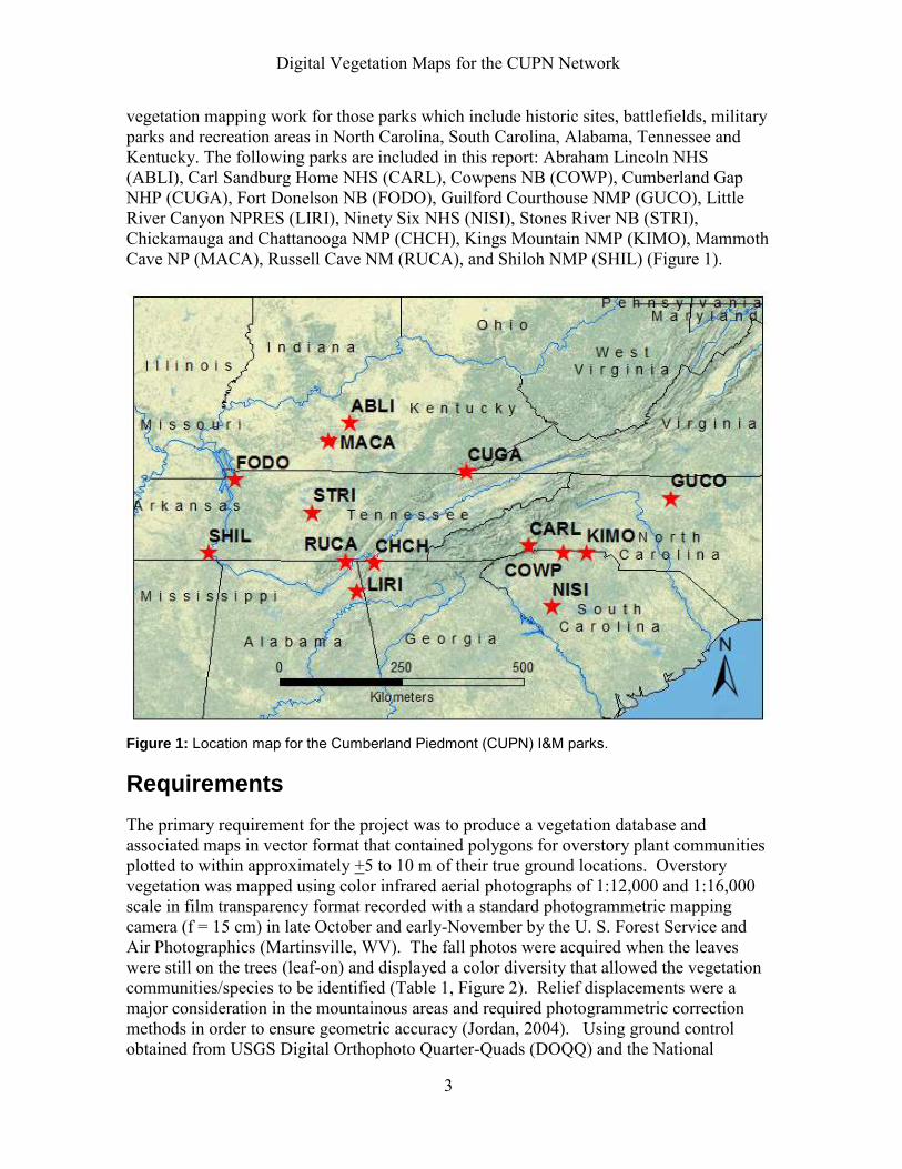
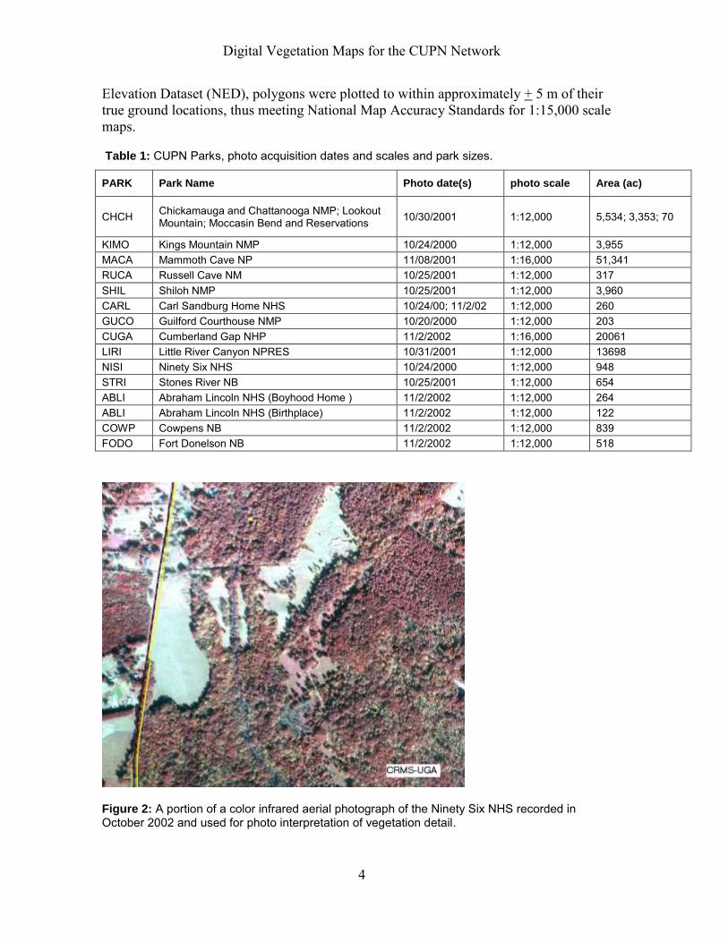

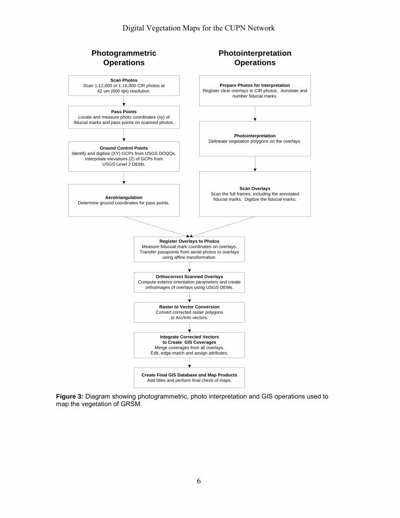


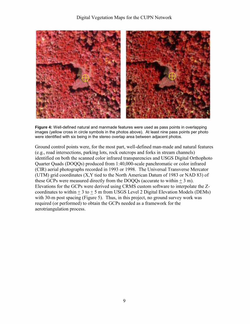


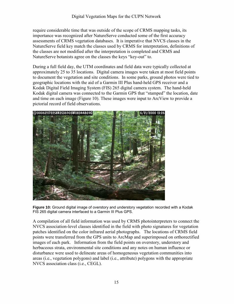


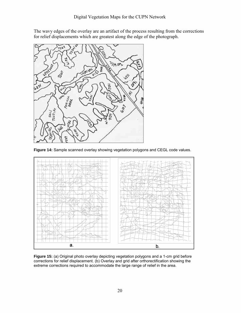

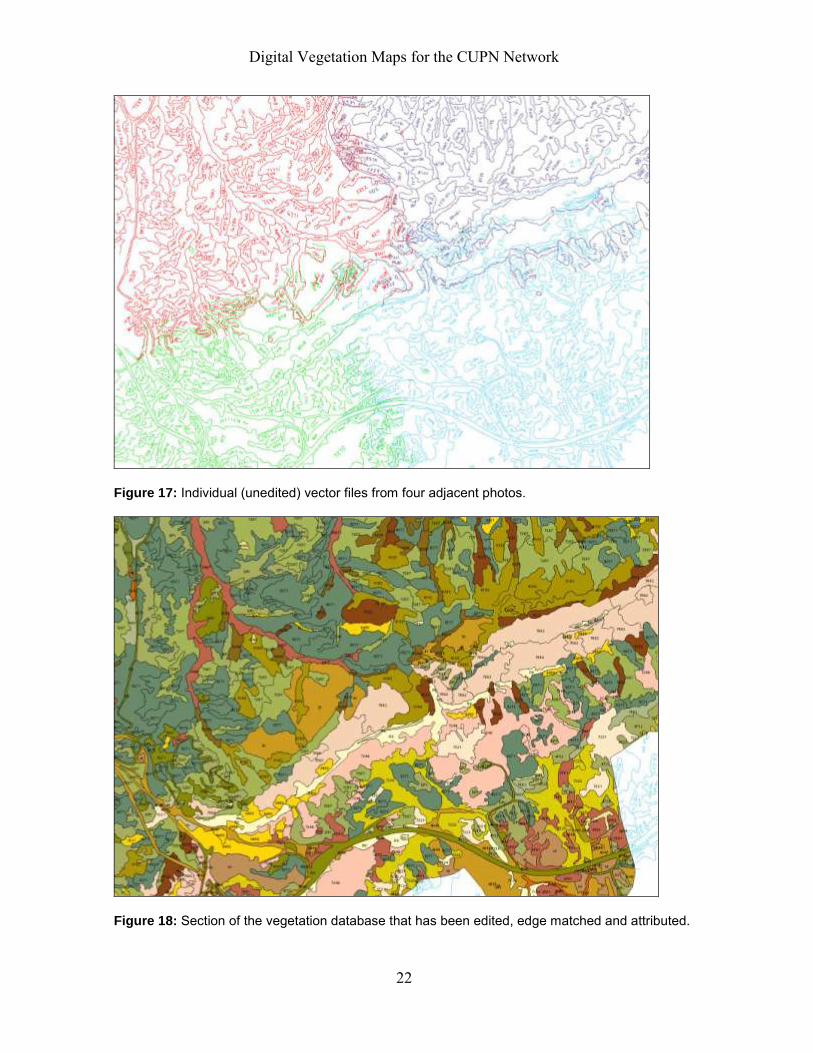


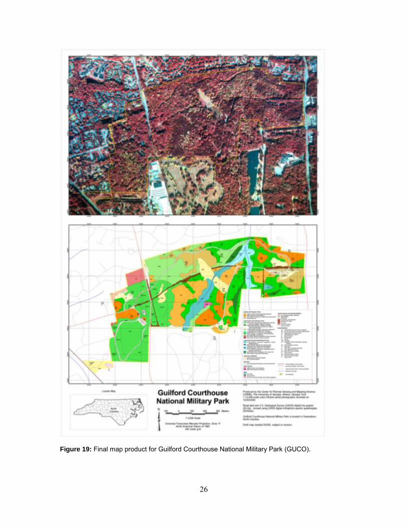


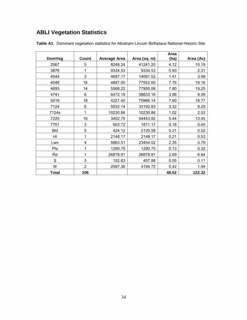


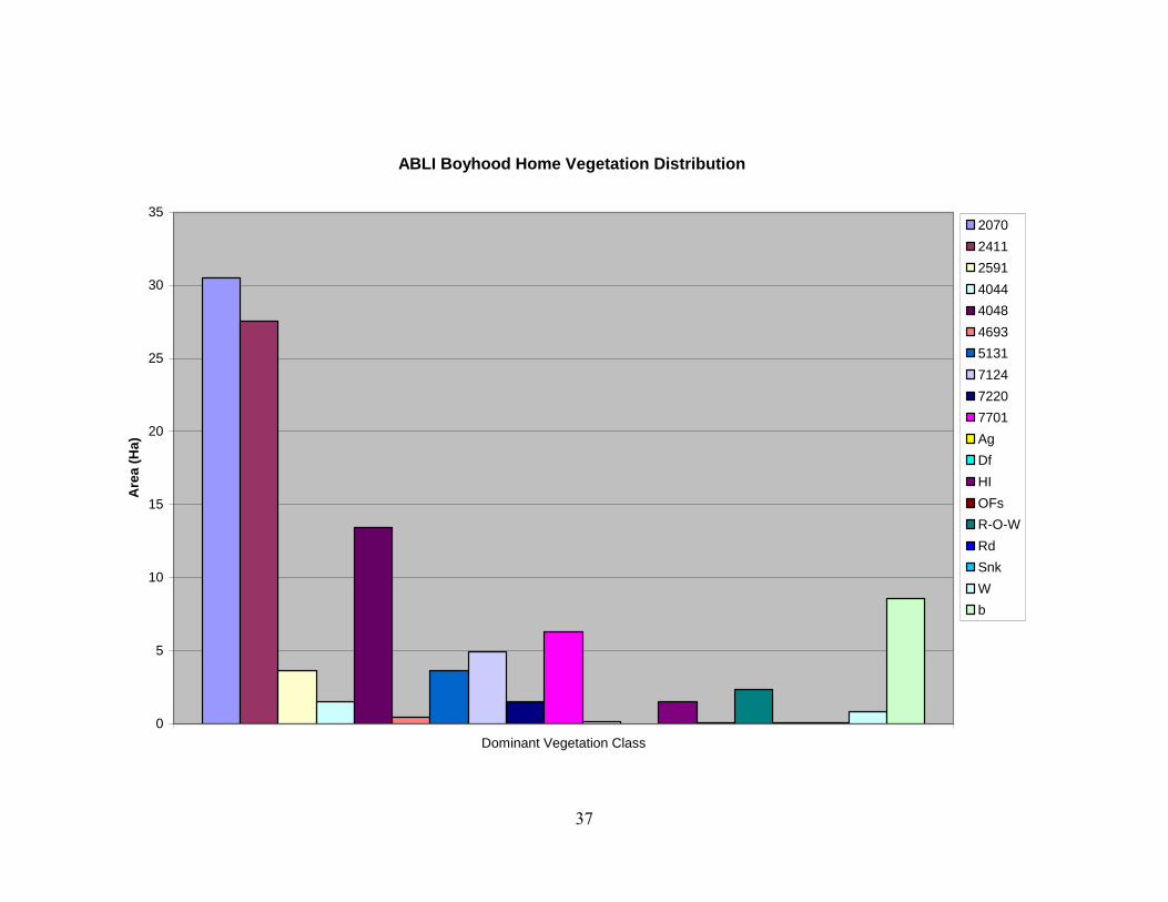


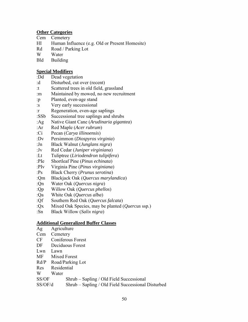


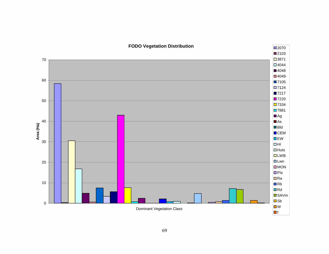
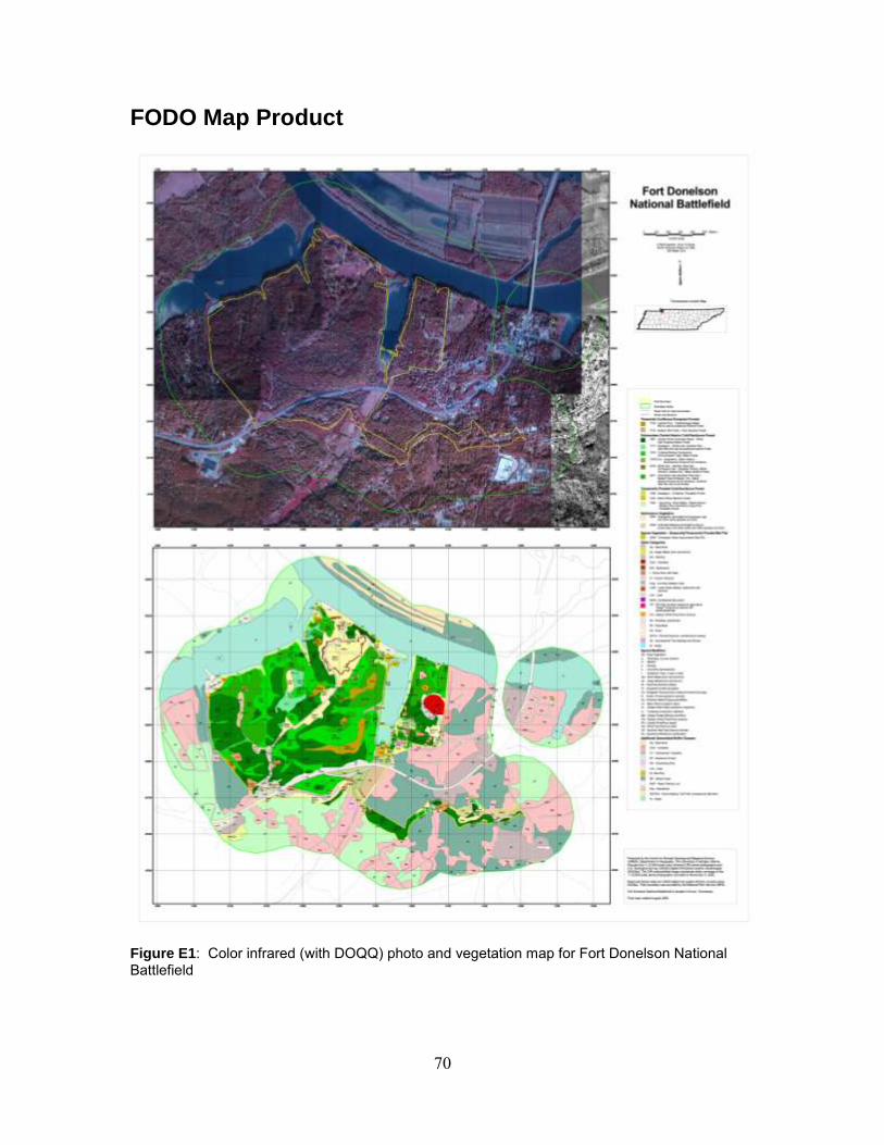


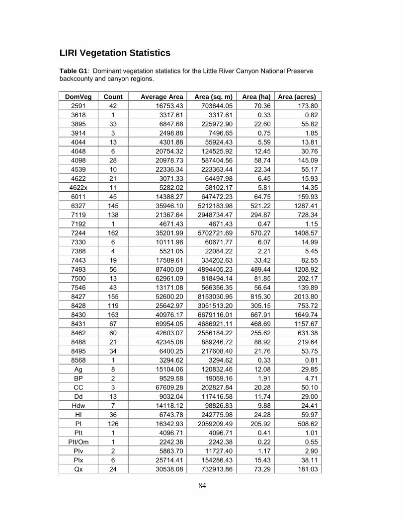

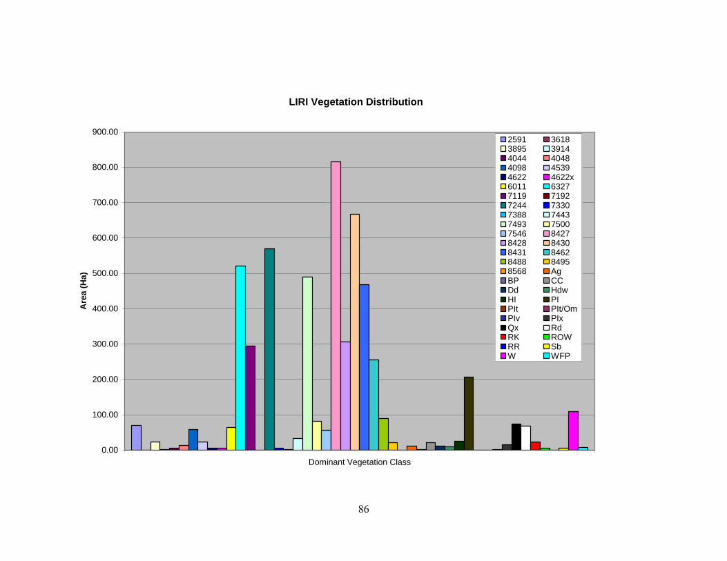
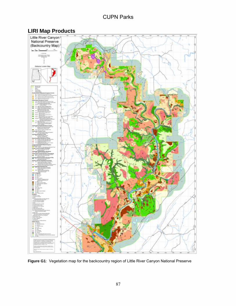

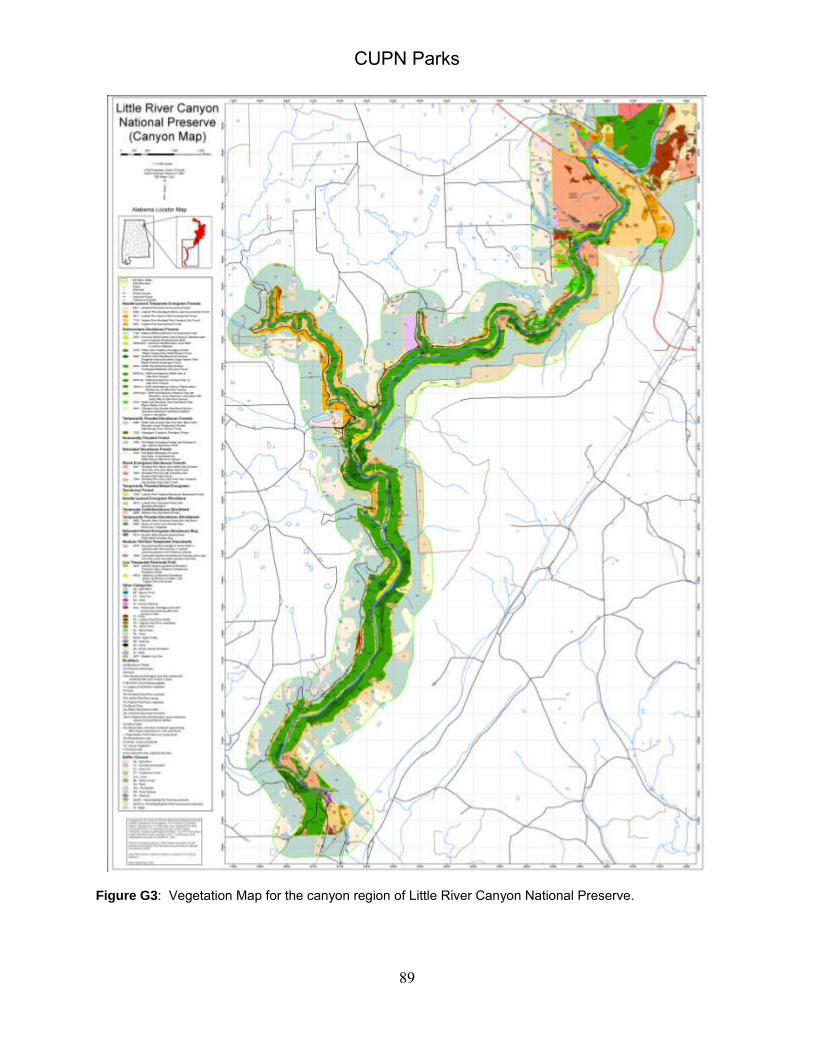

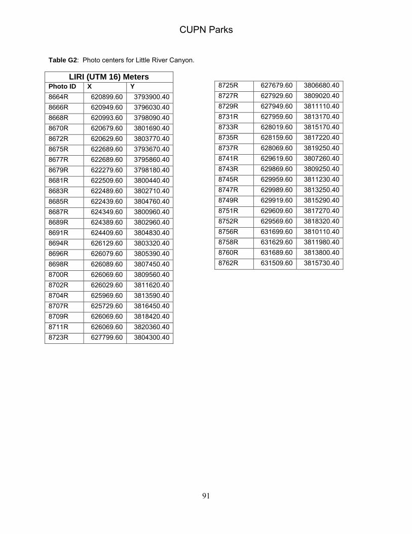


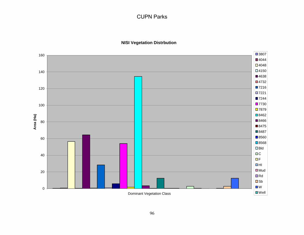

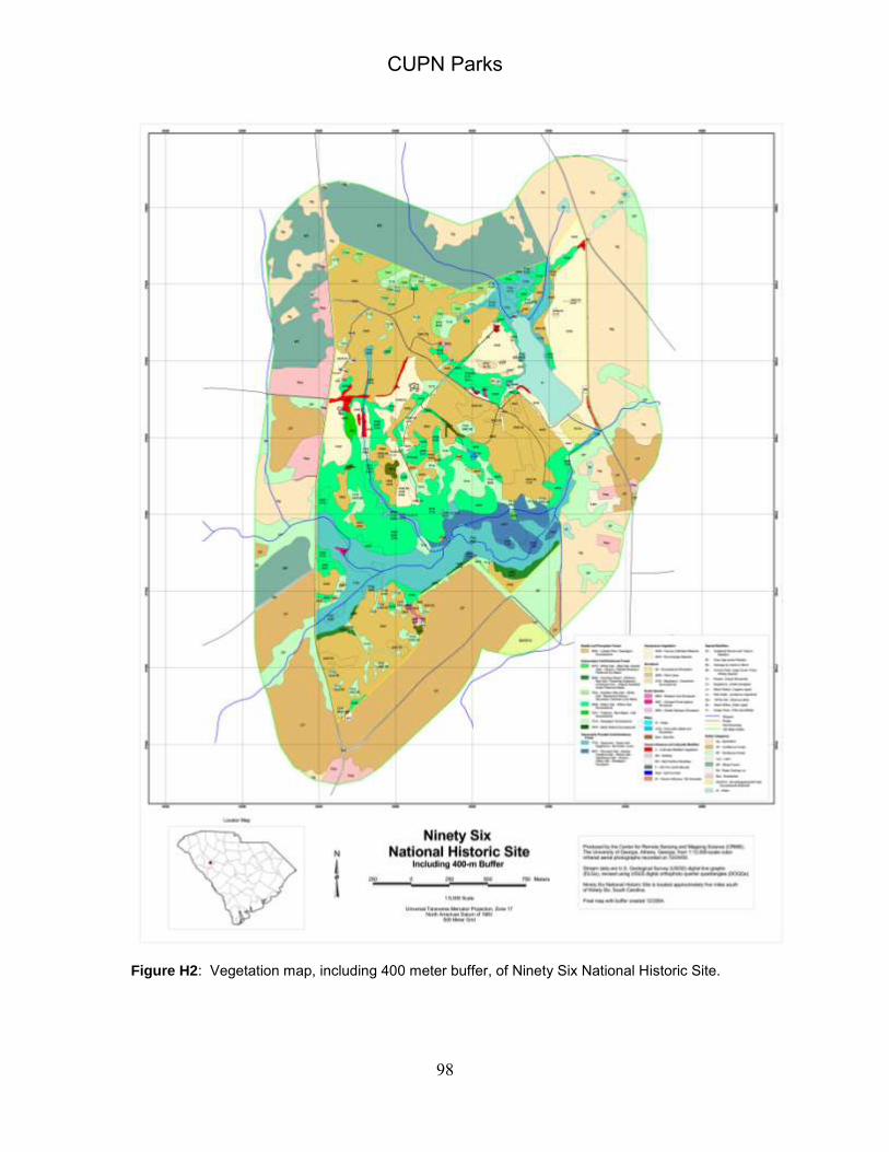

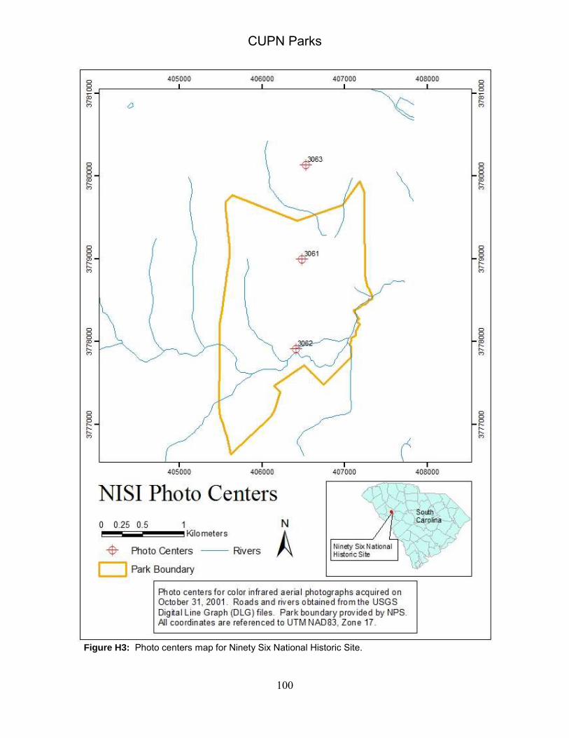


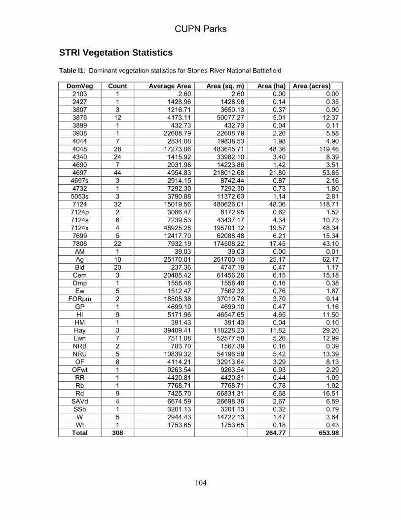
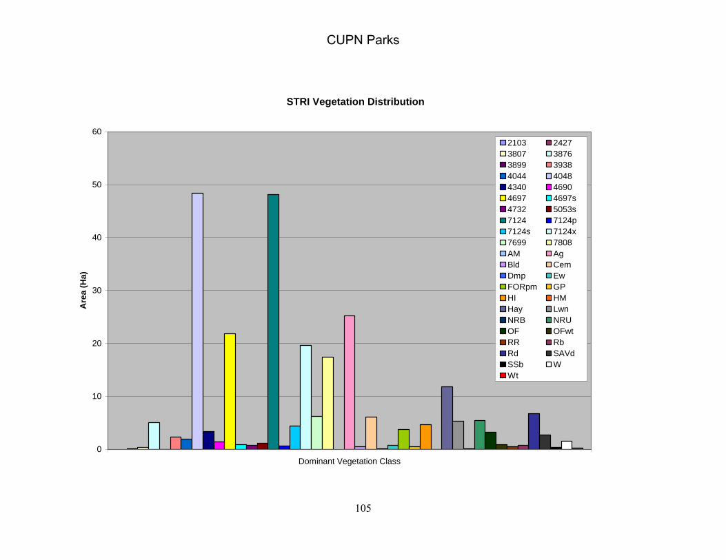


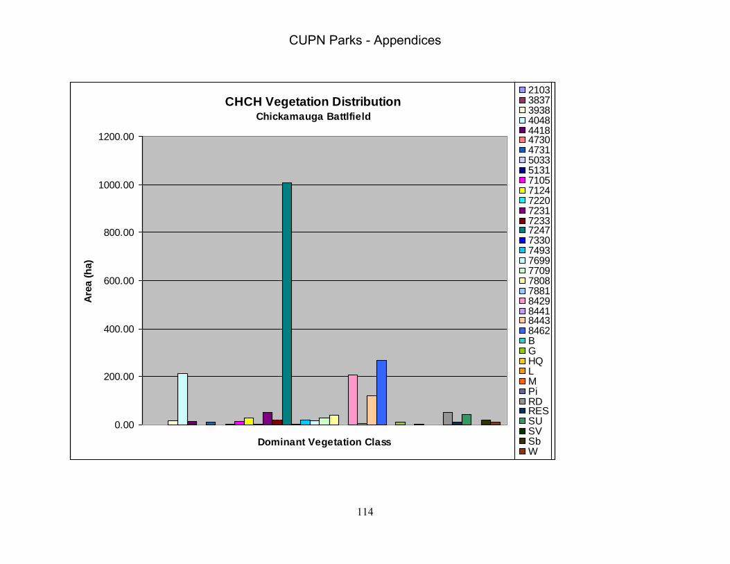


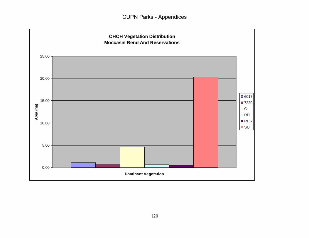
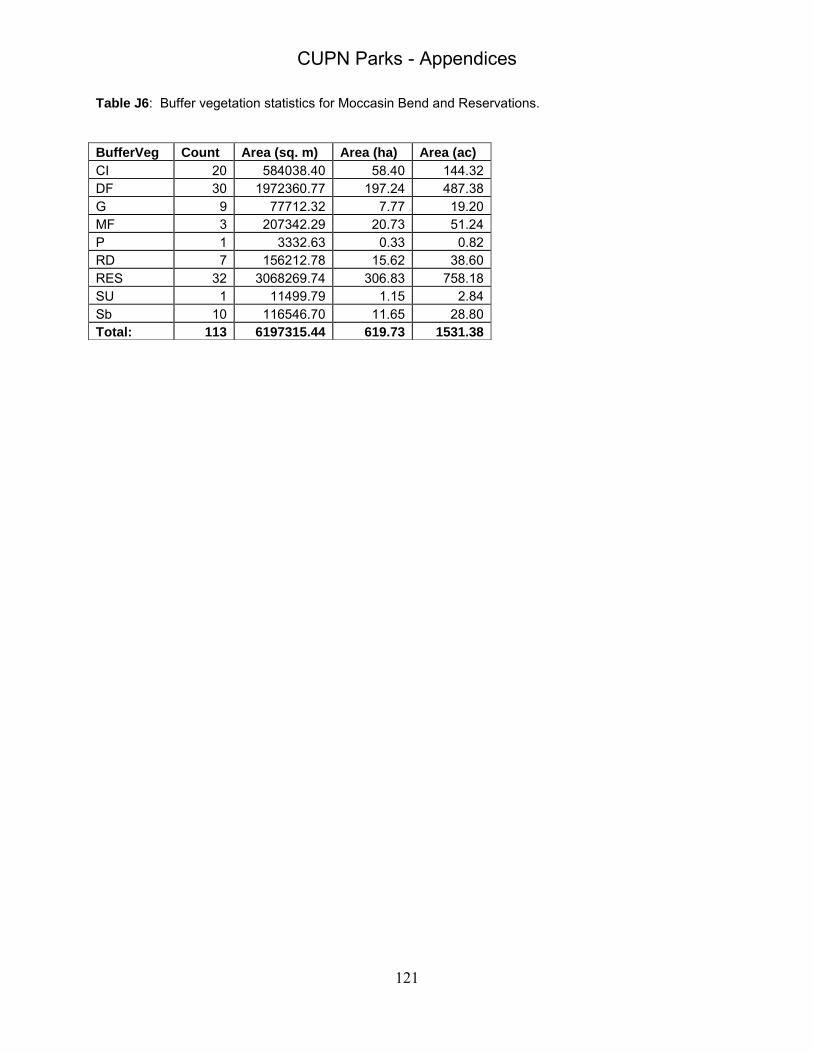


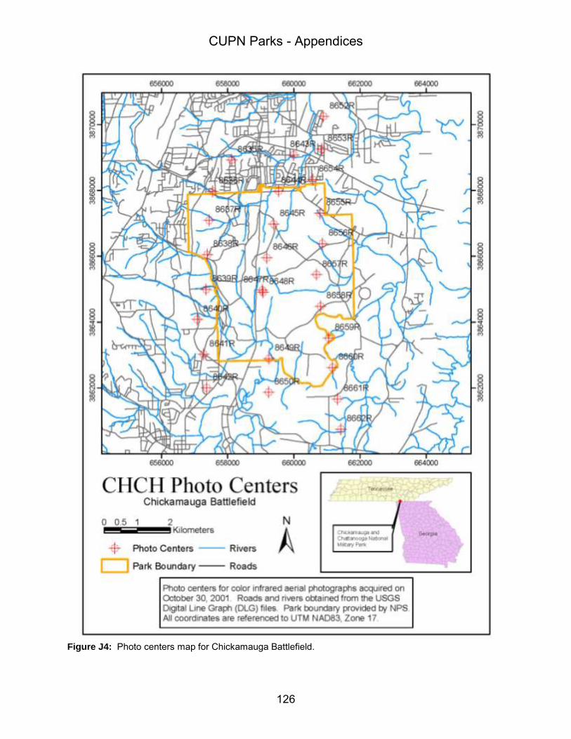


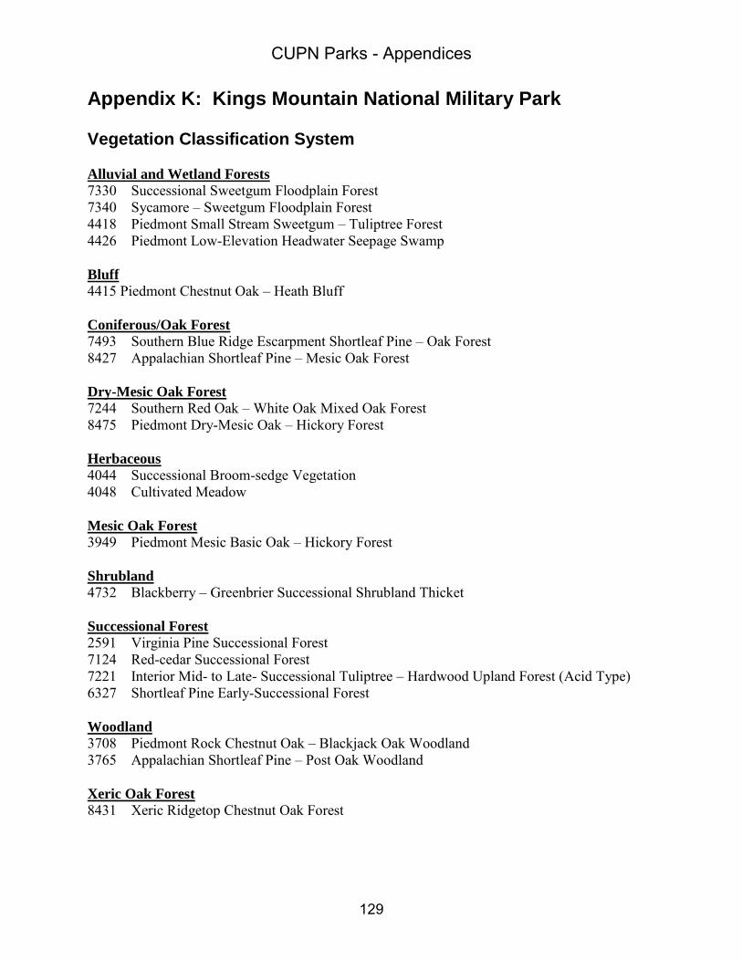


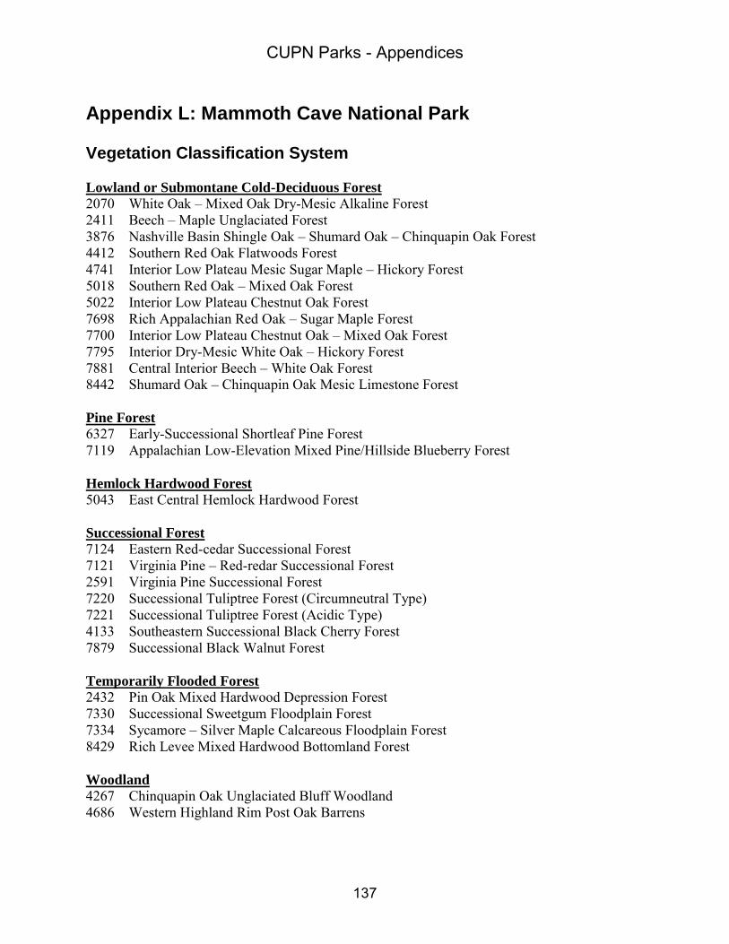

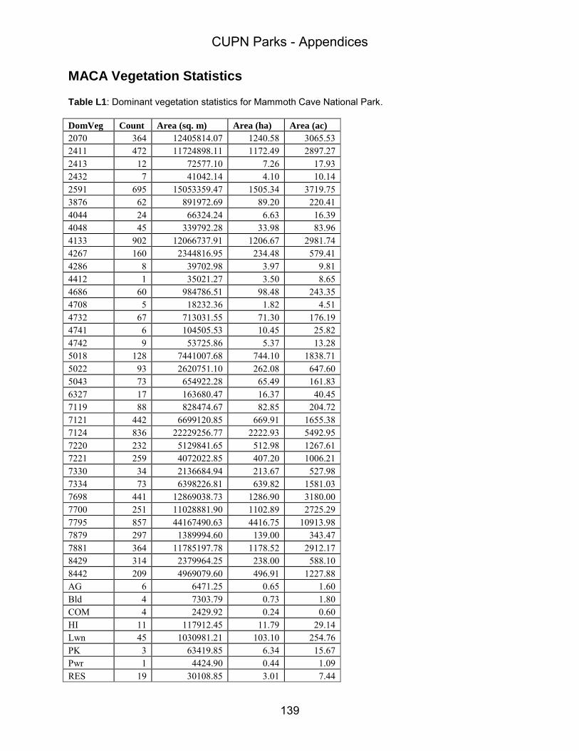


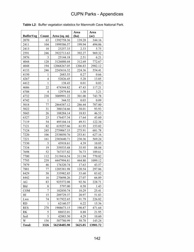
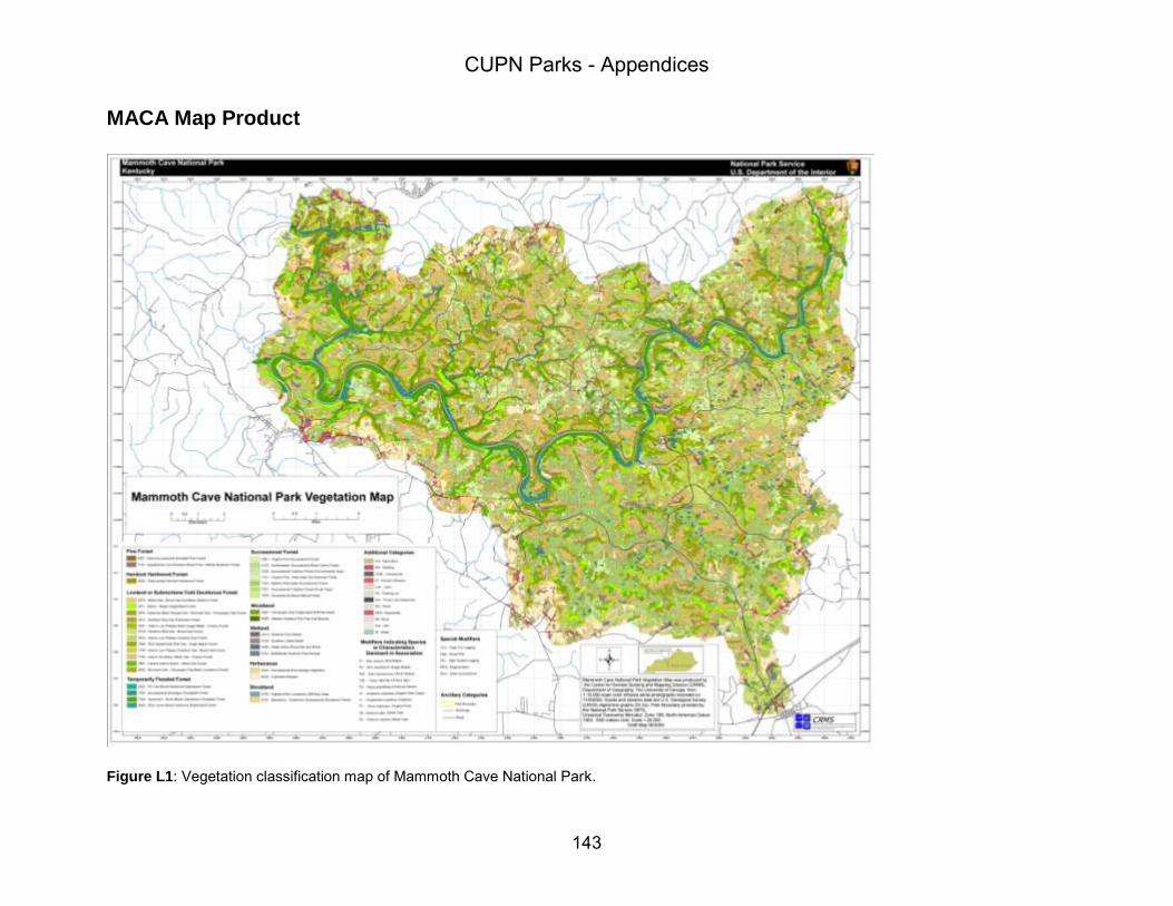


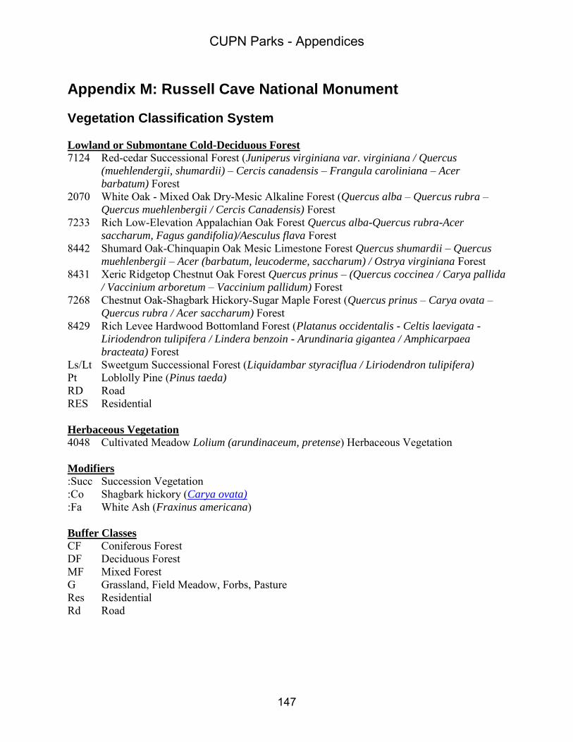
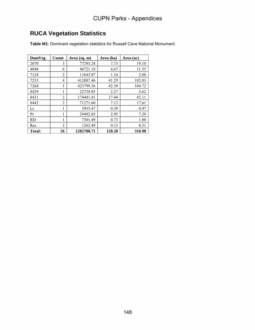


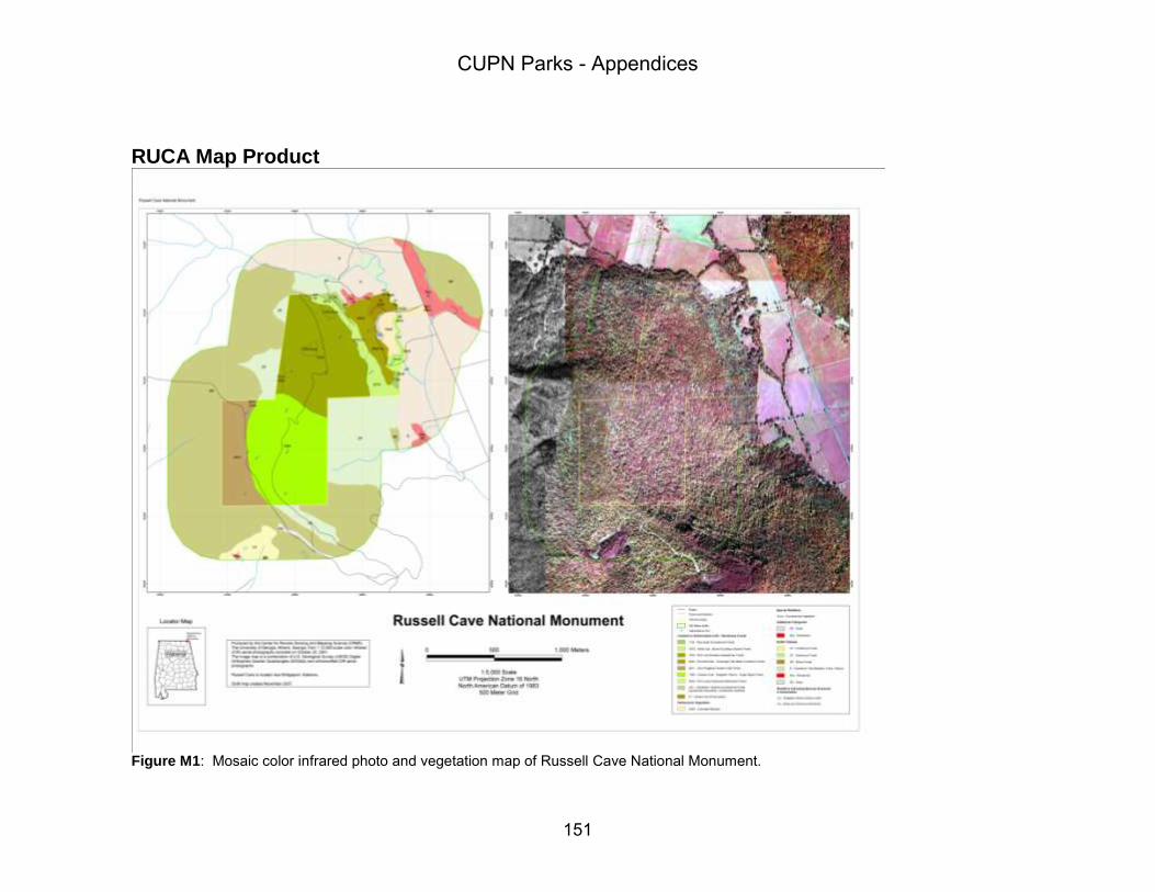


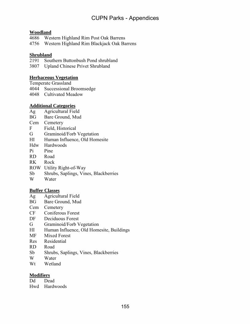


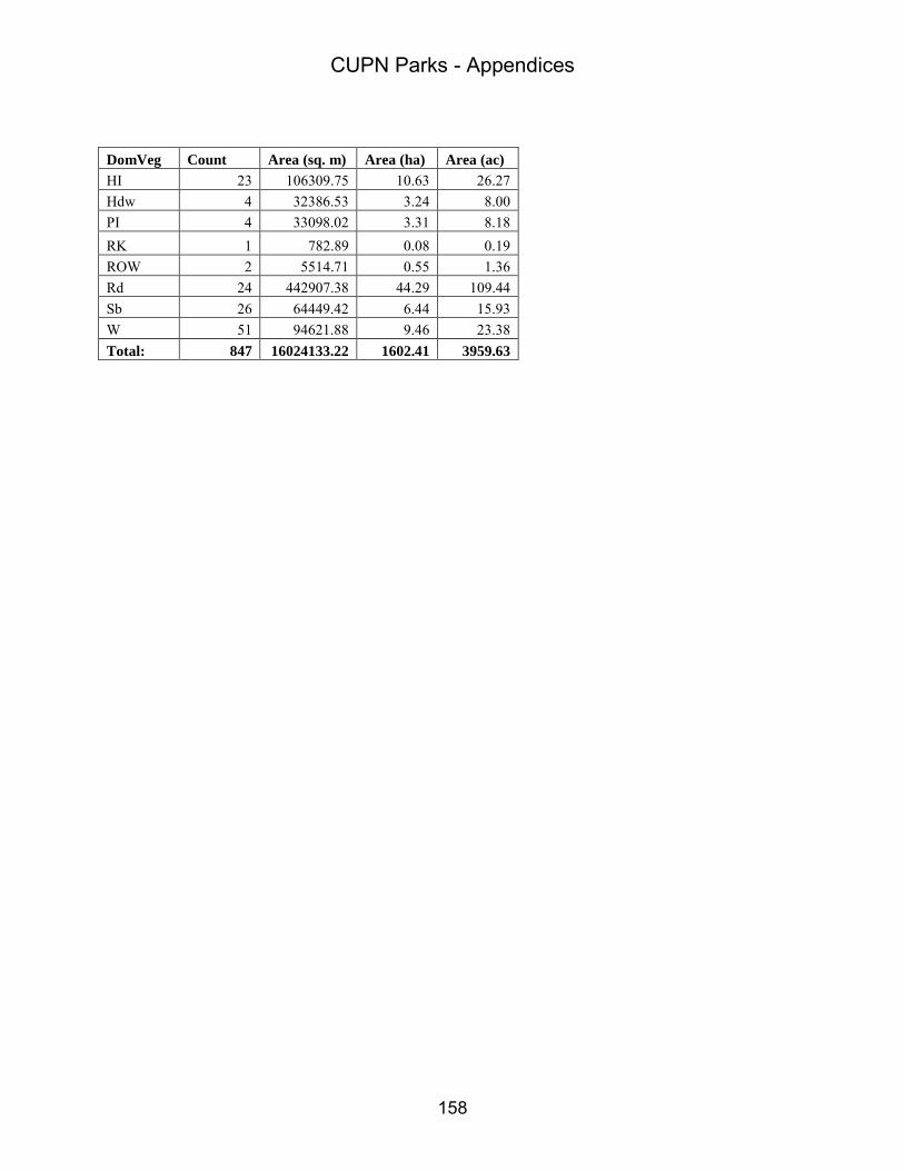
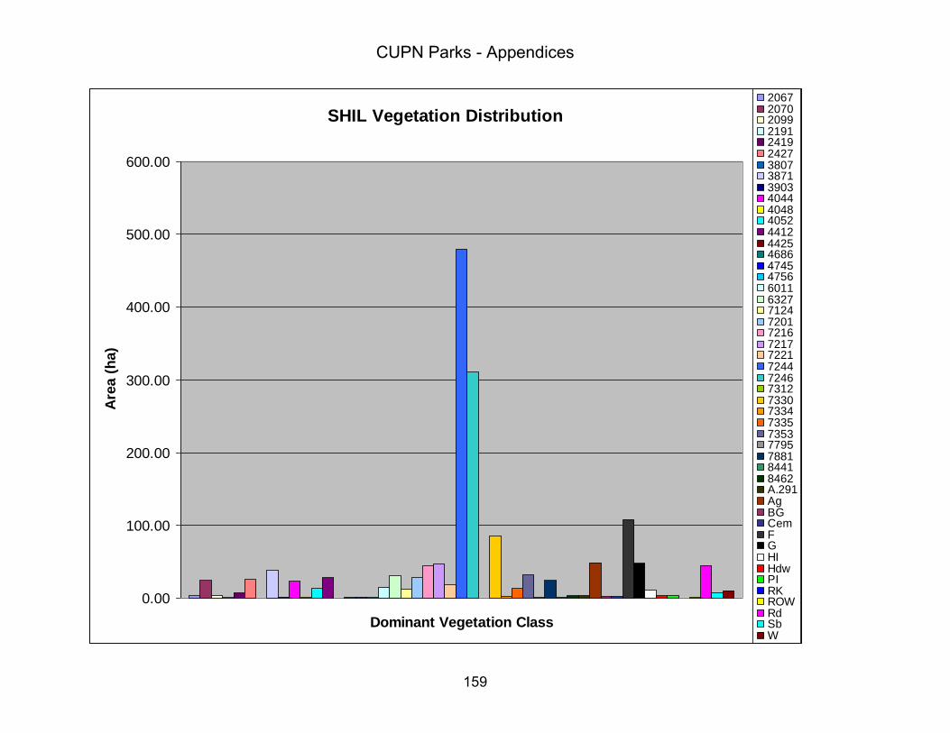
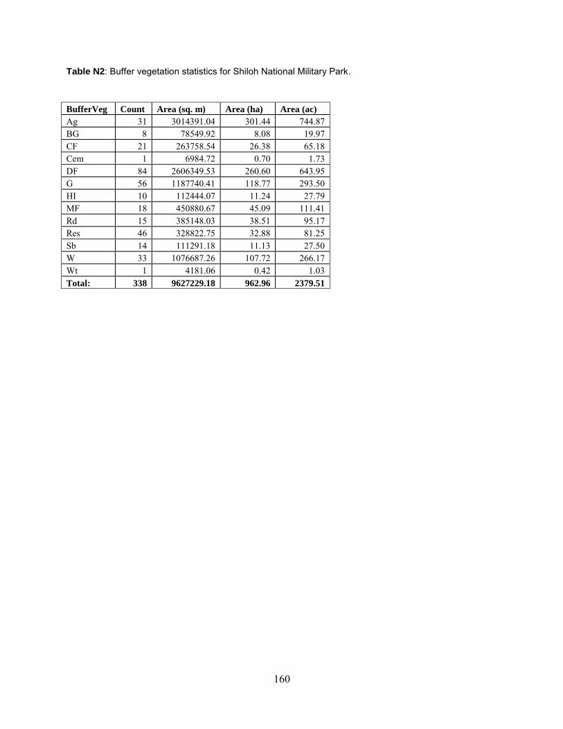


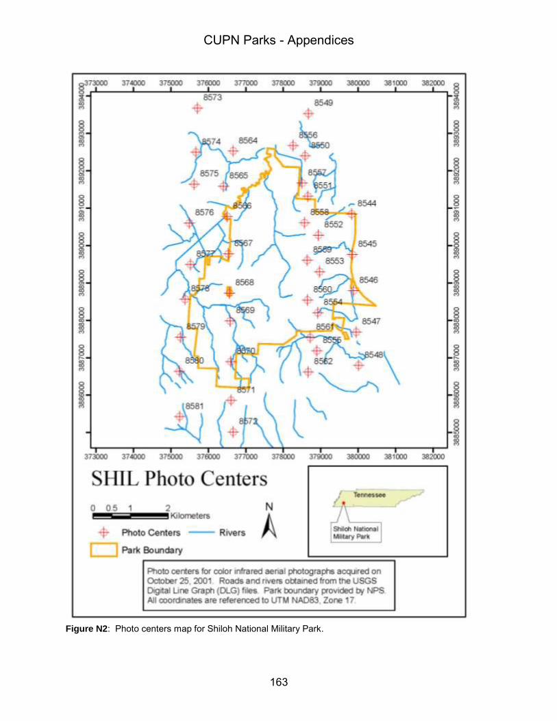


![[Vegetation and Remote Sensing] Vegetation](https://static.documents.pub/doc/80x56/577cdfd71a28ab9e78b21a32/vegetation-and-remote-sensing-vegetation.jpg)
