Differential Commuting Operator and Closed-Form Eigenfunctions for Linear Canonical Transforms Soo-Chang Pei 1,∗ and Chun-Lin Liu 2 1,2 Department of Electrical Engineering, National Taiwan University, No. 1, Sec. 4, Roosevelt Road, Taipei 10617, Taiwan ∗ Corresponding author: [email protected]The linear canonical transform (LCT) with a, b, c, d parameter plays an important role in quantum mechanics, optics, and signal processing. The eigenfunctions of the LCT are also important because they describe the self-imaging phenomenon in optical systems. However, the existing solutions for the eigenfunctions of the LCT are divided into many cases and they lack a systematic way to solve these eigenfunctions. In this paper, we find a linear, second-order, self-adjoint differential commuting operator that commutes with the linear canonical transform operator. Hence, the commuting operator and the LCT share the same eigenfunctions with different eigenvalues. The commuting operator is very general and simple when it is compared to the existing multiple-parameter differential equations. Then, the eigenfunctions can be derived systematically. The eigenvalues of the commuting operator have closed-form relationships with the eigenvalues of the LCT. We also simplify the eigenfunctions for |a + d| > 2 and a + d = ±2, b = 0 into the more compact closed form instead of the integral form. For |a + d| > 2, the eigenfunctions are related to the parabolic cylinder functions. c 2013 Optical Society of America OCIS codes: 070.0070, 070.2580, 070.2590, 070.2575. 1. Introduction Linear canonical transform (LCT) is a phase space integral transform that is a function of several real parameters, a, b, c, and d, where ad − bc = 1. LCT is a generalization of Fourier transform, fractional Fourier transform (FrFT), Fresnel transform, scaling operation, and chirp multiplication operation [1–3]. It is also called canonical transforms [3], generalized 1
Transcript
Differential Commuting Operator and Closed-Form
Eigenfunctions for Linear Canonical Transforms
Soo-Chang Pei1,∗ and Chun-Lin Liu2
1,2Department of Electrical Engineering, National Taiwan University, No. 1, Sec. 4,
Linear canonical transform (LCT) is a phase space integral transform that is a function of
several real parameters, a, b, c, and d, where ad− bc = 1. LCT is a generalization of Fourier
transform, fractional Fourier transform (FrFT), Fresnel transform, scaling operation, and
chirp multiplication operation [1–3]. It is also called canonical transforms [3], generalized
1
Fresnel transforms [4], ABCD transforms [5], or quadratic-phase integrals [1]. The LCT
finds useful applications in quantum mechanics, optics, digital holography, and signal pro-
cessing. In quantum mechanics, FrFT can be used for solving the time-dependent Schrodinger
equation [3, 6, 7]. The first-order optical systems can be analyzed by LCT [1, 5, 8]. Speckle
metrology systems and spatial coherence were designed and analyzed by Yura et al. using the
LCT [9, 10]. In digital holography, the LCT finds application in understanding the filtering
role of CCD pixels and finite apertures [11]. LCT also twists the time-frequency representa-
tion of the signal so we can perform time-frequency analysis [1] and filter design [12]. A full
study on the fractional Fourier transform and the Wigner distribution function is referred
to [13].
The eigenfunctions of LCT have been known for many years. In [4], the eigenfunctions
of LCT were studied. The closed-form solutions are in the form of scaled Hermite Gaussian
functions multiplied by the chirp functions [4]. However, the solutions are valid only when |a+d| < 2. In [14,15], the eigenfunctions for all cases were discussed. However, the eigenfunctions
for different cases are quite different. It seems that there are no general-forms for all these
distinct eigenfunctions. In addition, some eigenfunctions are expressed in integral forms. For
instance, when |a+d| > 2, the solution is related to the self-similar functions, or fractals [16].
There is no closed-form solution for these self-similar functions so The final eigenfunction is
described as integrals. Recently, the eigenfunction of the LCT for |a+d| > 2 was derived to be
a complex-scaled Hermite Gaussian function with a chirp term, which is unbounded [17,18].
In this paper, we take a different point of view on the eigenfunctions and then complete
the study of eigenfunctions in [14]. We find a linear operator CM which commutes with LCT
operator. As a result, CM and LCT operator share common eigenfunctions with different
eigenvalues. This operator is the linear combination of D2t , tDt + Dtt, and t2 with proper
combination coefficients, where Dt = d /d t is the differential operator. This commuting
operator always has the same general form with arbitrary a, b, c, and d parameters. However,
the eigenvalues of CM vary for different a, b, c, and d. We show that the eigenvalues of CMare related to the eigenvalues of LCT by certain formulae. The operator CM is shown to be
a self-adjoint operator so that the eigenfunctions are orthonormal, whatever the parameters
a, b, c, and d are. With the help of CM, we complete the study of the eigenfunctions in [14].
Notably, for |a + d| > 2, the solution can be expressed in terms of the parabolic cylinder
functions, which are generalizations of the Hermite Gaussian eigenfunctions in the |a+d| < 2
case.
This paper is summarized as follows. First, in Section 2, LCT and its eigenfunctions are
briefly reviewed for clarity. The linear operator CM is defined and its many properties are
investigated in Section 3. In Section 4, the complete study on the eigenfunctions of LCT is
given based on both CM and the previous results. We prove that our results are consistent
2
with the previous work and, in addition, these eigenfunctions are not only with closed forms
but are also orthonormal. In Section 5, we discuss the symmetry relations among the all
eigenvalues and eigenfunctions and give a short example to explain the physical meaning of
the solution. A comparison is made to distinguish our eigenfunctions for a+ d > 2 and those
in [17,18]. Section 6 points out some signal processing applications of the eigenfunctions of the
LCT, including an illustrative example to clarify the role of eigenfunction in implementing
the LCT. Finally, in Section 7, we summarize the result and make a conclusion.
2. Preliminary
2.A. Linear Canonical Transforms
LCT is defined for b 6= 0 by the following integral
XM(u) = (LMx) (u)
=
√
1
j2πb
∫ ∞
−∞x(t)ej
a2bt2e−j
1btuej
d2bu2 d t, b 6= 0, t, u ∈ R. (1)
The LCT can also be regarded as a transformation mapping from x to XM. In this paper,
we write the transformed result as XM(t) to facilitate the discussion about the operators.
When b = 0, the definition is modified into
XM(t) =√dej
cd2t2x(td), b = 0. (2)
The 2-by-2 matrix M = [a, b; c, d] is a real-valued matrix with det (M) = 1. The operator
LM, or sometimes denoted by La,b,c,d, is the linear canonical transform operator. The degree
of freedom of LCT is three with the constraint det (M) = 1.
The LCT has the additive property and the reversible property.
LM1M2 = LM1LM2 , L−1M
= LM−1. (3)
These properties enable us to decompose LCT with arbitrary M into the product of some
basic elementary operations [19]. Implementing these basic operations step by step gives us
the final result.
These basic operations are all special cases of LCT. They are summarized as follows:
1. Fourier transform (FT) corresponds the LCT with M = [0, 1;−1, 0]. Note that there
is an extra phase term√j in front of the conventional Fourier transform.
2. Fractional Fourier transform (FrFT) with fractional order α ∈ [0, 2π) [1, 7, 15] is the
LCT with M = [cosα, sinα;− sinα, cosα], still with the constant phase term,√j. Our
definition is consistent with that in [15].
3
3. Fresnel transform is obtained from the LCT with M = [1, b; 0, 1]. In optics, Fresnel
transform describes the wave propagation in free space [20]. In signal processing or
time-frequency analysis, this case is also called chirp convolution operation.
4. Scaling operation corresponds the LCT with M = [σ−1, 0; 0, σ]. From (2), the scaling
operation is then√σx(σt).
5. Chirp multiplication operation is derived from the LCT with M = [1, 0; c, 1]. In this
case, the operation is ejc2t2x(t).
All of the relationships and the details about these special transforms can be found in [1,3].
The LCT has lots of mathematical properties. We want to note the multiplication-by-t
property and the derivative property specifically (see Chapter 2 in [15] and Section 3.4 in [1]),
which are
LM {tx(t)} =
(
jbd
d t+ td
)
XM(t), (4)
LM
{
d
d tx(t)
}
=
(
ad
d t− jct
)
XM(t), (5)
where the left-hand side x(t) denotes the original signal and the right-hand side XM(t) stands
for its LCT. (4) and (5) can be further rewritten as the operator form by
LMt = (jbDt + td)LM, (6)
LMDt = (aDt − jct)LM. (7)
These two identities will be used throughout this paper. For other LCT properties, we refer
to the reader to [1].
2.B. Previous Work on the Eigenfunctions of LCT
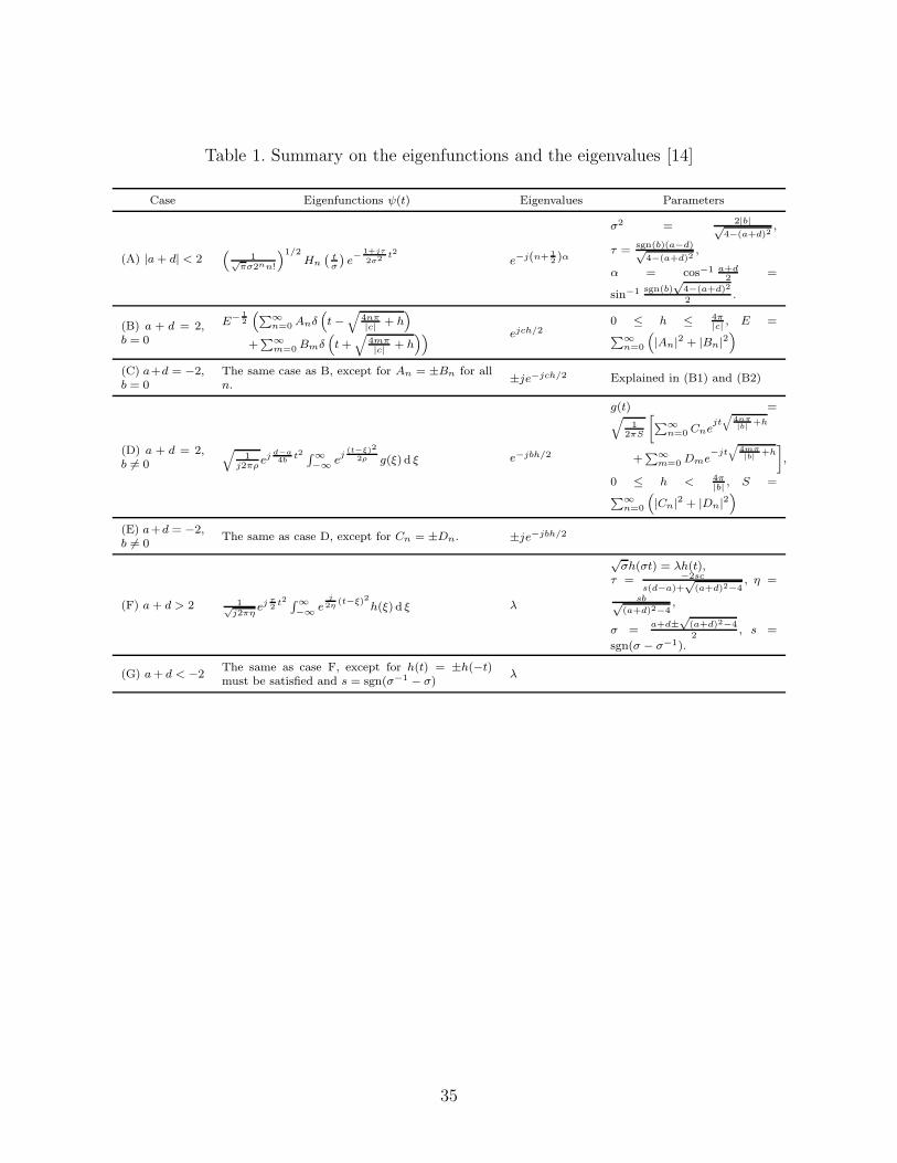
The eigenfunctions and the eigenvalues of LCT were studied very extensively in [14]. They
are divided into seven cases and summarized in Table 1.
The eigenfunctions are first divided by the value of a+d and then by the value of b. In Case
(A) for |a+d| < 2, the solution is the product of the scaled Hermite Gaussian function and the
chirp function, as indicated in the Case (A) of Table 1. In this case, the eigenfunctions form
a complete and orthonormal basis for L2(R) [4], where L2(R) ={
x(t)|∫∞−∞ |x(t)|2 d t <∞
}
is the set of finite-energy functions. Hence the eigenfunctions are very suitable for several
applications in optics [4].
In Case (B) and Case (C), the eigenfunctions are impulse trains with the amplitude An for
the right-shifted impulses, and with the amplitude Bm for the left-shifted impulses. In Case
(D) and Case (E), the function g(t) is the linear combination of two complex exponential
4
functions but g(t) is not the eigenfunction. The actual eigenfunction is an integral associated
with g(t). In addition, in Case (C) and Case (E), the combination coefficients satisfy An =
±Bn or Cn = ±Dn.
In Case (F), the eigenfunction is connected with the function h(t), which is the self-similar
function, or fractals. The closed-form h(t) and the corresponding eigenvalue λ are unknown
and not given. As a result, the eigenfunction is left as an open problem to solve. Case (G)
limits h(t) to be even or odd functions and the rest part is similar to Case (F).
The existing results still require to be elaborated in terms of the eigenfunctions, eigen-
values, and their properties. First of all, the eigenfunctions can be further simplified into
closed forms instead of being represented in integral forms. To do so, it is possible to find the
closed-form expression of self-similar signals and then evaluate the integral in Case (D) and
Case (F). Secondly, in Case (F), if b = 0, we have η = 0 and the chirp function in the integral
becomes undefined. It is more likely to discuss this special case separately. Finally, because
we only discuss the real-parameter LCT in this paper, then LM is an unitary operator, which
implies that all the eigenfunctions are orthogonal. However, in the existing literature, the
orthogonality of the eigenfunctions is not addressed, except for Case (A).
In [18], for |a+d| > 2, the complex-scaled Hermite Gaussian function is the eigenfunction,
Ψ(σ,τ)n (u) =
1√
σ2nn!√jπHn
( u
σejπ4
)
ej1−τ
2σ2 u2
, (8)
However, the eigenfunction is not bounded as u approaches infinity,∣
∣
∣Ψ
(σ,τ)n (u)
∣
∣
∣→ ∞ as u→
∞. This divergent property prevents the eigen-decomposition of the LCT. Our goal is to find
a bounded solution in this case and compare the both solutions.
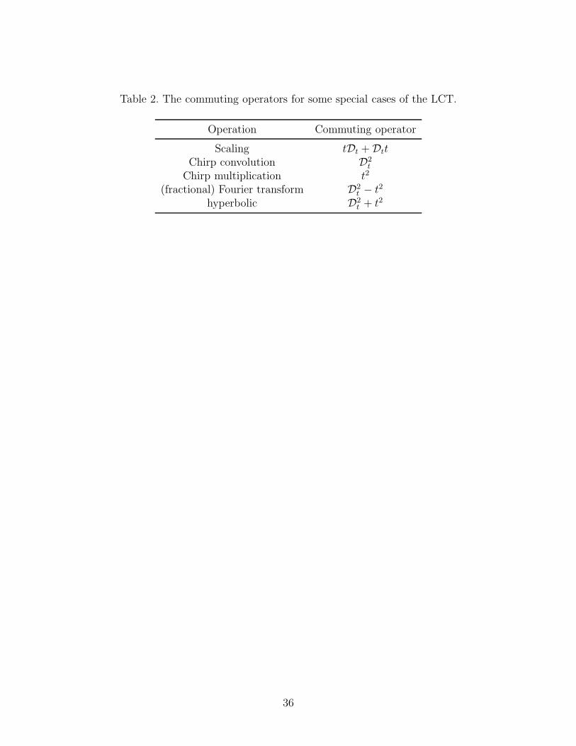
3. General commuting operator CMIn [1, 3], the commuting operators for some special cases of the LCT are listed in Table 2.
These operators commute with LCT operator for different cases. The commuting operator
and LCT share the common eigenfunctions with different eigenvalues. Hence, we can solve
the commuting operator to have the eigenfunctions of LCT. This technique has been widely
used in the study of the eigenfunctions of discrete Fourier transforms [21, 22].
However, the conventional commuting operators in Table 2 are not suitable for the general
LCT with arbitrary a, b, c, and d. Our goal is to find a general expression for the commuting
operator, so that we can directly obtain the eigenfunctions by solving the general commuting
operator. It is observed that the existing commuting operators are the linear combination of
the three basic operators:D2t , tDt+Dtt, and t
2. Hence, we assume that the general commuting
operator is the linear combination of them. The combination coefficients are directly related
to the parameters a, b, c, and d.
5
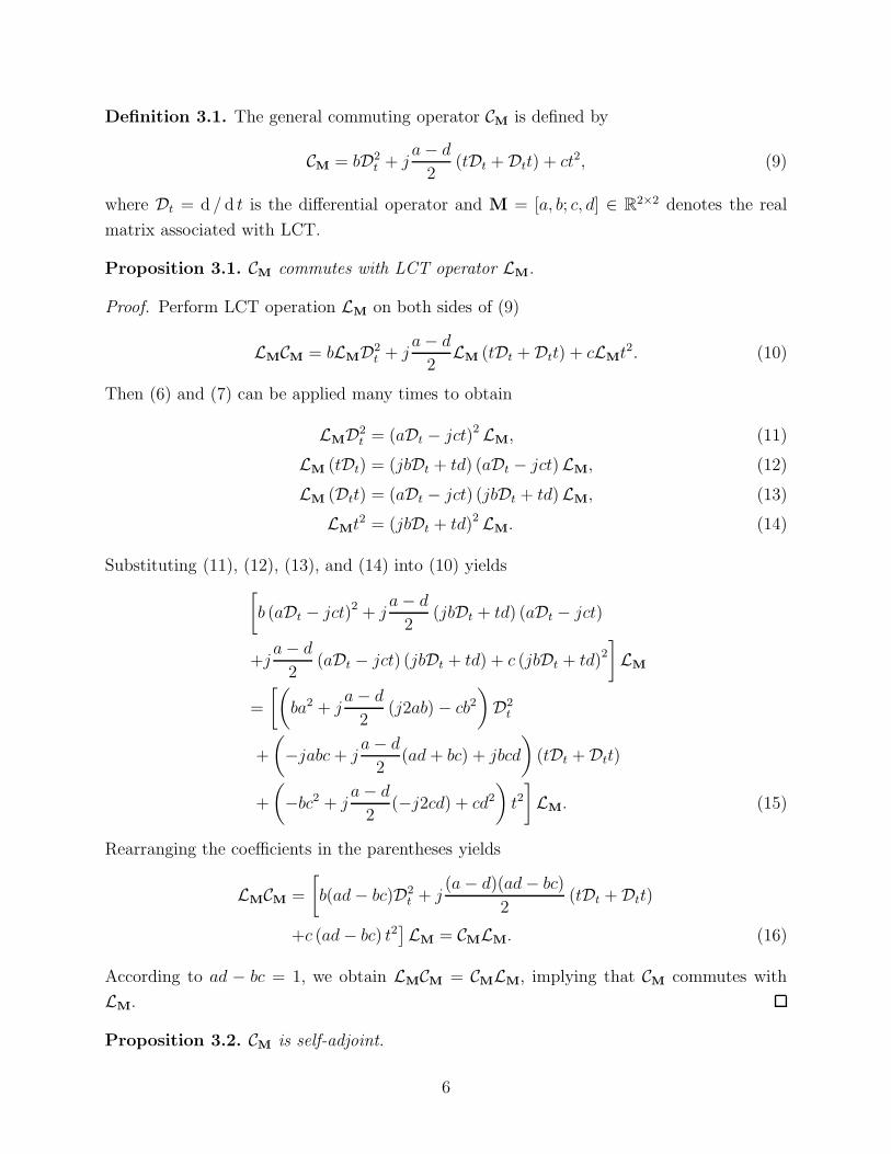
Definition 3.1. The general commuting operator CM is defined by
CM = bD2t + j
a− d
2(tDt +Dtt) + ct2, (9)
where Dt = d / d t is the differential operator and M = [a, b; c, d] ∈ R2×2 denotes the real
matrix associated with LCT.
Proposition 3.1. CM commutes with LCT operator LM.
Proof. Perform LCT operation LM on both sides of (9)
LMCM = bLMD2t + j
a− d
2LM (tDt +Dtt) + cLMt
2. (10)
Then (6) and (7) can be applied many times to obtain
LMD2t = (aDt − jct)2 LM, (11)
LM (tDt) = (jbDt + td) (aDt − jct)LM, (12)
LM (Dtt) = (aDt − jct) (jbDt + td)LM, (13)
LMt2 = (jbDt + td)2 LM. (14)
Substituting (11), (12), (13), and (14) into (10) yields
[
b (aDt − jct)2 + ja− d
2(jbDt + td) (aDt − jct)
+ja− d
2(aDt − jct) (jbDt + td) + c (jbDt + td)2
]
LM
=
[(
ba2 + ja− d
2(j2ab)− cb2
)
D2t
+
(
−jabc + ja− d
2(ad+ bc) + jbcd
)
(tDt +Dtt)
+
(
−bc2 + ja− d
2(−j2cd) + cd2
)
t2]
LM. (15)
Rearranging the coefficients in the parentheses yields
LMCM =
[
b(ad− bc)D2t + j
(a− d)(ad− bc)
2(tDt +Dtt)
+c (ad− bc) t2]
LM = CMLM. (16)
According to ad − bc = 1, we obtain LMCM = CMLM, implying that CM commutes with
LM.
Proposition 3.2. CM is self-adjoint.
6
Proof. Assume that A† and B† stands for the adjoint operator of the operator A and B,respectively. The basic operation rules for adjoint operators are
(A+ B)† = A† + B†, (AB)† = B†A†. (17)
In addition, the some useful adjoint operators are
D†t = −Dt,
(
D2t
)†= D2
t , t† = t, a† = a∗, (18)
where a is a complex number and ∗ denotes complex conjugates. To prove that CM is self-
adjoint, taking the adjoint operator of CM gives us
C†M
=(
bD2t
)†+
[
ja− d
2(tDt +Dtt)
]†+(
ct2)†
(19)
=(
D2t
)†b† + (tDt +Dtt)
†(
ja− d
2
)†+(
t2)†c†. (20)
Note that (19) and (20) are due to the basic operation rules (17). The next step is to apply
the known adjoint operators, listed in (18), one by one. Therefore, CM can be simplified into
C†M
= bD2t + (−tDt −Dtt)
(
−j a− d
2
)
+ ct2, (21)
where the parameters a, b, c, and d are all real numbers. Rearranging (21) yields C†M
=
CM.
It is concluded from Proposition 3.1 that CM and LM have a common set of eigenfunctions
with different eigenvalues. Assume that the common eigenfunctions are written as ψµM(t).
By definition, we have
CMψµM(t) = µMψµM(t), LMψµM(t) = λMψµM(t), (22)
where µM is the eigenvalue of CM and λM is the eigenvalue of LM. It is noted that µM is not
the same as λM because they correspond different operators. We write the subscript µM in
the eigenfunctions in order to specify that the eigenfunctions depend on µM.
Then, according to Proposition 3.2 and the fact that LM is unitary, we have four major
properties
Property 1. The eigenvalues µM are all real.
Property 2. The eigenfunctions ψµM(t) are orthogonal to each other.
Property 3. The eigenfunctions ψµM(t) form a complete set.
7
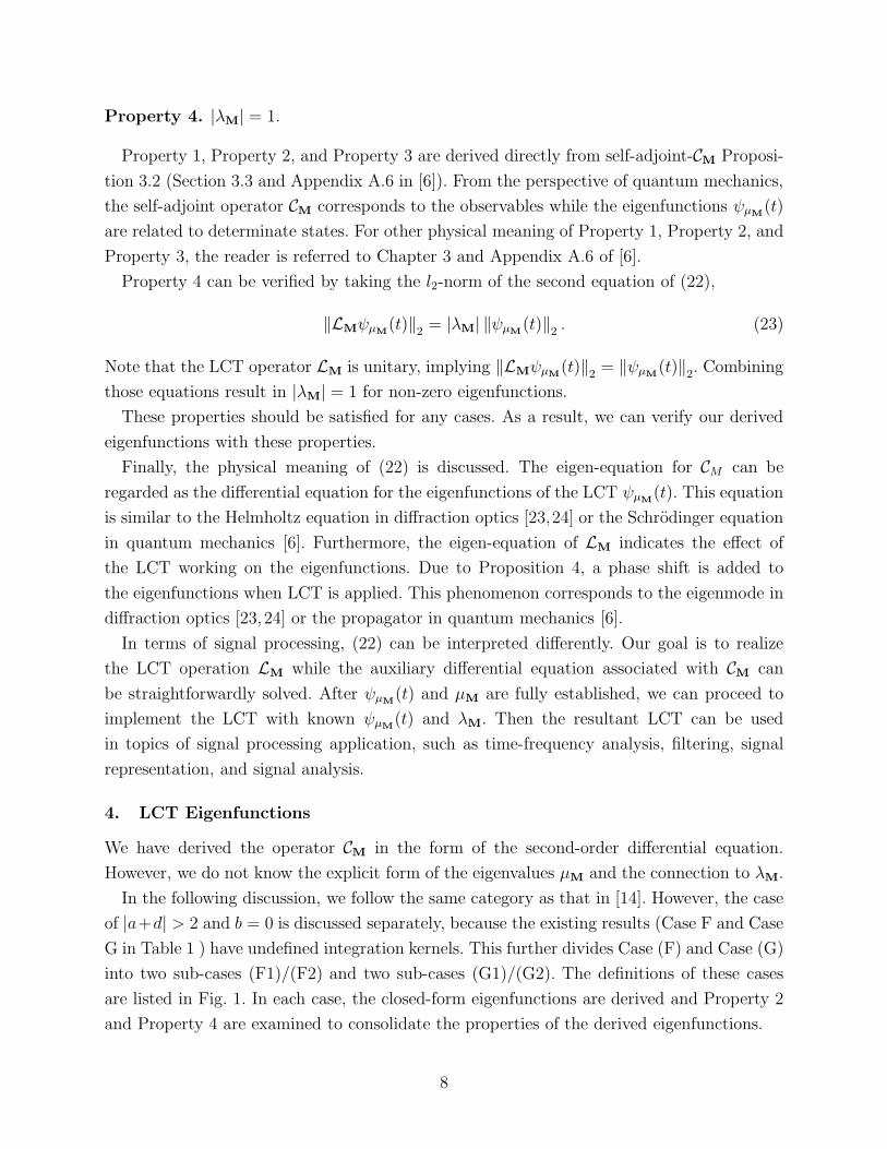
Property 4. |λM| = 1.
Property 1, Property 2, and Property 3 are derived directly from self-adjoint-CM Proposi-
tion 3.2 (Section 3.3 and Appendix A.6 in [6]). From the perspective of quantum mechanics,
the self-adjoint operator CM corresponds to the observables while the eigenfunctions ψµM(t)
are related to determinate states. For other physical meaning of Property 1, Property 2, and
Property 3, the reader is referred to Chapter 3 and Appendix A.6 of [6].
Property 4 can be verified by taking the l2-norm of the second equation of (22),
‖LMψµM(t)‖2 = |λM| ‖ψµM(t)‖2 . (23)
Note that the LCT operator LM is unitary, implying ‖LMψµM(t)‖2 = ‖ψµM(t)‖2. Combining
those equations result in |λM| = 1 for non-zero eigenfunctions.
These properties should be satisfied for any cases. As a result, we can verify our derived
eigenfunctions with these properties.
Finally, the physical meaning of (22) is discussed. The eigen-equation for CM can be
regarded as the differential equation for the eigenfunctions of the LCT ψµM(t). This equation
is similar to the Helmholtz equation in diffraction optics [23,24] or the Schrodinger equation
in quantum mechanics [6]. Furthermore, the eigen-equation of LM indicates the effect of
the LCT working on the eigenfunctions. Due to Proposition 4, a phase shift is added to
the eigenfunctions when LCT is applied. This phenomenon corresponds to the eigenmode in
diffraction optics [23, 24] or the propagator in quantum mechanics [6].
In terms of signal processing, (22) can be interpreted differently. Our goal is to realize
the LCT operation LM while the auxiliary differential equation associated with CM can
be straightforwardly solved. After ψµM(t) and µM are fully established, we can proceed to
implement the LCT with known ψµM(t) and λM. Then the resultant LCT can be used
in topics of signal processing application, such as time-frequency analysis, filtering, signal
representation, and signal analysis.
4. LCT Eigenfunctions
We have derived the operator CM in the form of the second-order differential equation.
However, we do not know the explicit form of the eigenvalues µM and the connection to λM.
In the following discussion, we follow the same category as that in [14]. However, the case
of |a+d| > 2 and b = 0 is discussed separately, because the existing results (Case F and Case
G in Table 1 ) have undefined integration kernels. This further divides Case (F) and Case (G)
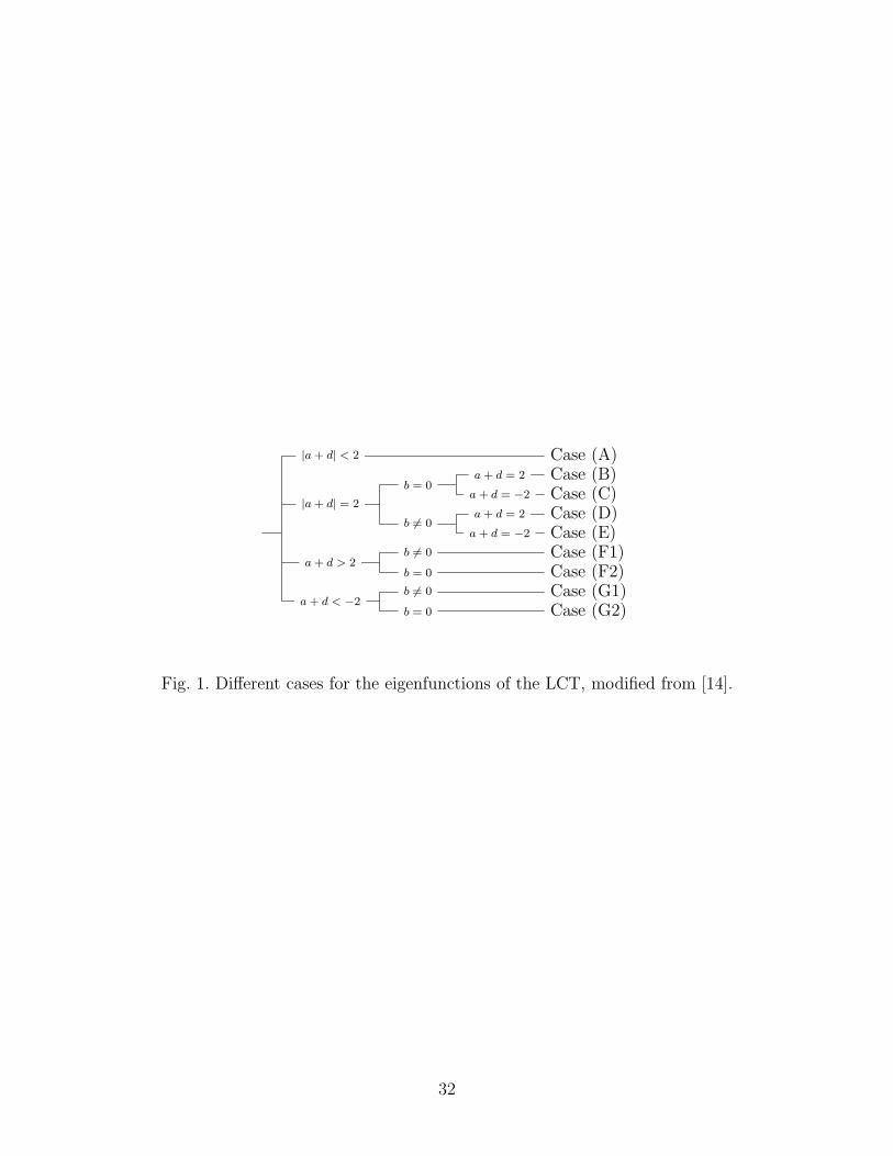
into two sub-cases (F1)/(F2) and two sub-cases (G1)/(G2). The definitions of these cases
are listed in Fig. 1. In each case, the closed-form eigenfunctions are derived and Property 2
and Property 4 are examined to consolidate the properties of the derived eigenfunctions.
8
4.A. Case (A): |a+ d| < 2
In case (A), the eigenfunctions and the eigenvalues are already known in [4] and they are sum-
marized in Case (A) of Table 1. In addition, the differential equations for the eigenfunctions
were also derived in [4], which are(
−1
2σ2D2
t − jτtDt +1 + τ 2
2σ2t2 − jτ
2
)
ψn(t)
= (n+ 1/2)ψn(t). (24)
Here we denote the eigenfunctions as ψn(t) because they depend on the parameter n =
0, 1, 2 . . . . Starting from (24), substituting parameter λ, σ, and τ into a, b, c, d, as summarized
in Case (A) of Table 1, and multiplying −(2b)/σ2 on both sides give us(
bD2t + j(a− d)tDt + ct2 − j
a− d
2
)
ψn(t)
= −(2b/σ2) (n+ 1/2)ψn(t), (25)
Also, because of the multiplication property of the differential operator, Dtt = tDt+I, whereIx(t) = x(t) is the identity operator, we arrange the above equation into
CMψn(t) =(
bD2t + j
a− d
2(tDt +Dtt) + ct2
)
ψn(t)
= −sgn(b)√
4− (a+ d)2 (n+ 1/2)ψn(t). (26)
Hence, the existing differential equations are matched with our general operator CM. The
eigenvalues µM are found to be
µM = −sgn(b)√
4− (a+ d)2 (n+ 1/2) . (27)
The next problem is to find the closed-form expression of λM in terms of µM. Still, from
the existing result in Table 1, we obtain
λM = e−j(n+1/2)α = (cosα + j sinα)−(n+1/2) . (28)
(28) is associated with parameters α and n. Substituting sinα, cosα into the form given in
Table 1, which are
cosα = (a + d)/2, (29)
sinα =1
2sgn(b)
√
4− (a+ d)2, (30)
and n+ 1/2 into µM by (27), λM can be written as
λM =
[
a+ d
2+ j
sgn(b)√
4− (a+ d)2
2
]
µM
sgn(b)√
4−(a+d)2
. (31)
9
The reason why λM is written as (31) is that we want to find the direct relationship among
a, b, c, d, µM and λM instead of defining other intermediate parameters such as σ, α, τ . In
other cases, we take this direct approach to derive the formula concerning µM and λM.
We briefly examine these results. The eigenfunctions have been known to be complete and
orthogonal [4]. According to (28), the eigenvalues |λM| = 1,
|λM| = |cosα + j sinα|−(n+1/2) = 1. (32)
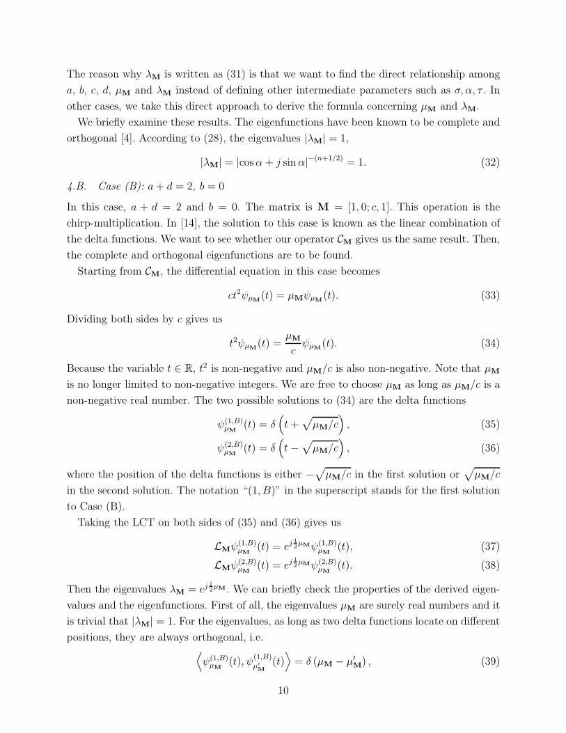
4.B. Case (B): a+ d = 2, b = 0
In this case, a + d = 2 and b = 0. The matrix is M = [1, 0; c, 1]. This operation is the
chirp-multiplication. In [14], the solution to this case is known as the linear combination of
the delta functions. We want to see whether our operator CM gives us the same result. Then,
the complete and orthogonal eigenfunctions are to be found.
Starting from CM, the differential equation in this case becomes
ct2ψµM(t) = µMψµM(t). (33)
Dividing both sides by c gives us
t2ψµM(t) =µM
cψµM(t). (34)
Because the variable t ∈ R, t2 is non-negative and µM/c is also non-negative. Note that µM
is no longer limited to non-negative integers. We are free to choose µM as long as µM/c is a
non-negative real number. The two possible solutions to (34) are the delta functions
ψ(1,B)µM
(t) = δ(
t+√
µM/c)
, (35)
ψ(2,B)µM
(t) = δ(
t−√
µM/c)
, (36)
where the position of the delta functions is either −√
µM/c in the first solution or√
µM/c
in the second solution. The notation “(1, B)” in the superscript stands for the first solution
to Case (B).
Taking the LCT on both sides of (35) and (36) gives us
LMψ(1,B)µM
(t) = ej12µMψ(1,B)
µM(t), (37)
LMψ(2,B)µM
(t) = ej12µMψ(2,B)
µM(t). (38)
Then the eigenvalues λM = ej12µM . We can briefly check the properties of the derived eigen-
values and the eigenfunctions. First of all, the eigenvalues µM are surely real numbers and it
is trivial that |λM| = 1. For the eigenvalues, as long as two delta functions locate on different
positions, they are always orthogonal, i.e.⟨
ψ(1,B)µM
(t), ψ(1,B)µ′M
(t)⟩
= δ (µM − µ′M) , (39)
10
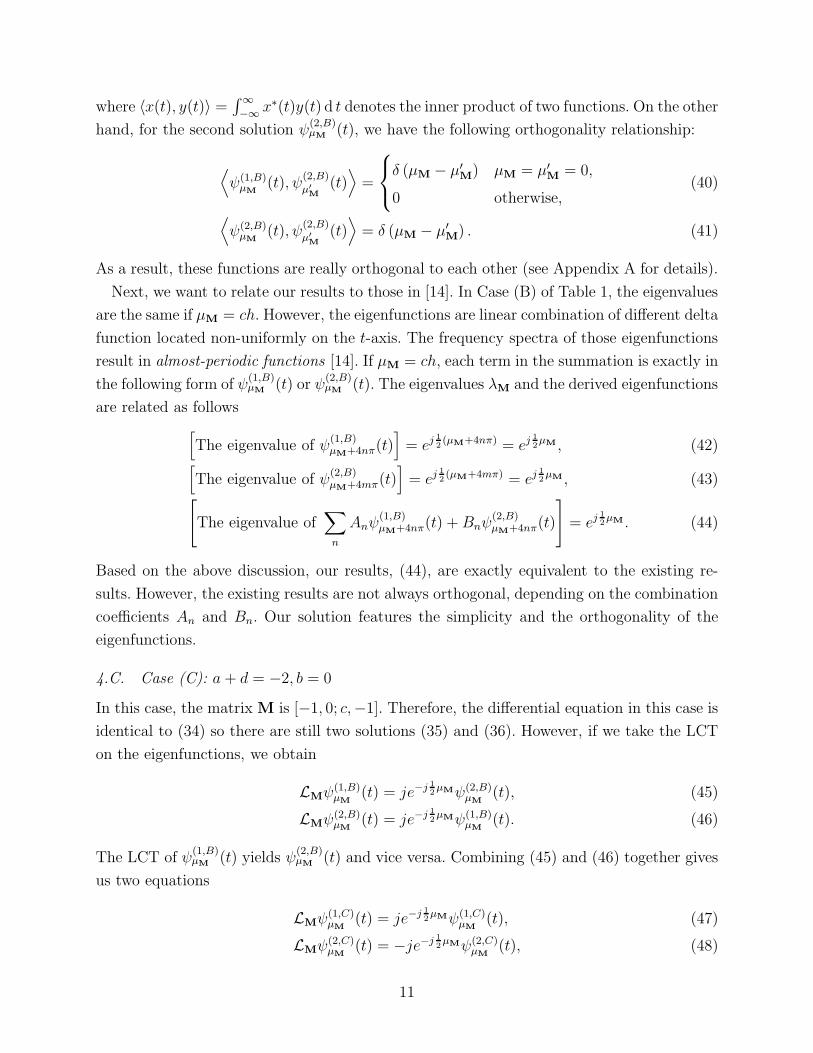
where 〈x(t), y(t)〉 =∫∞−∞ x∗(t)y(t) d t denotes the inner product of two functions. On the other
hand, for the second solution ψ(2,B)µM (t), we have the following orthogonality relationship:
⟨
ψ(1,B)µM
(t), ψ(2,B)µ′M
(t)⟩
=
δ (µM − µ′M) µM = µ′
M= 0,
0 otherwise,(40)
⟨
ψ(2,B)µM
(t), ψ(2,B)µ′M
(t)⟩
= δ (µM − µ′M) . (41)
As a result, these functions are really orthogonal to each other (see Appendix A for details).
Next, we want to relate our results to those in [14]. In Case (B) of Table 1, the eigenvalues
are the same if µM = ch. However, the eigenfunctions are linear combination of different delta
function located non-uniformly on the t-axis. The frequency spectra of those eigenfunctions
result in almost-periodic functions [14]. If µM = ch, each term in the summation is exactly in
the following form of ψ(1,B)µM (t) or ψ
(2,B)µM (t). The eigenvalues λM and the derived eigenfunctions
are related as follows
[
The eigenvalue of ψ(1,B)µM+4nπ(t)
]
= ej12(µM+4nπ) = ej
12µM , (42)
[
The eigenvalue of ψ(2,B)µM+4mπ(t)
]
= ej12(µM+4mπ) = ej
12µM , (43)
[
The eigenvalue of∑
n
Anψ(1,B)µM+4nπ(t) +Bnψ
(2,B)µM+4nπ(t)
]
= ej12µM . (44)
Based on the above discussion, our results, (44), are exactly equivalent to the existing re-
sults. However, the existing results are not always orthogonal, depending on the combination
coefficients An and Bn. Our solution features the simplicity and the orthogonality of the
eigenfunctions.
4.C. Case (C): a + d = −2, b = 0
In this case, the matrix M is [−1, 0; c,−1]. Therefore, the differential equation in this case is
identical to (34) so there are still two solutions (35) and (36). However, if we take the LCT
on the eigenfunctions, we obtain
LMψ(1,B)µM
(t) = je−j12µMψ(2,B)
µM(t), (45)
LMψ(2,B)µM
(t) = je−j12µMψ(1,B)
µM(t). (46)
The LCT of ψ(1,B)µM (t) yields ψ
(2,B)µM (t) and vice versa. Combining (45) and (46) together gives
us two equations
LMψ(1,C)µM
(t) = je−j12µMψ(1,C)
µM(t), (47)
LMψ(2,C)µM
(t) = −je−j 12µMψ(2,C)
µM(t), (48)
11
where
ψ(1,C)µM
(t) =1√2
(
ψ(1,B)µM
(t) + ψ(2,B)µM
(t))
, (49)
ψ(2,C)µM
(t) =1√2
(
ψ(1,B)µM
(t)− ψ(2,B)µM
(t))
. (50)
According to (47) and (48), ψ(1,C)µM (t) and ψ
(2,C)µM (t) are all eigenfunctions. Besides, we notice
that the eigenvalues are λ(1,C)M
= je−j12µM for the first solution and λ
(2,C)M
= −je−j 12µM for the
second solution. It is trivial to show that µM are real, |λ(1,C)M
| = |λ(2,C)M
| = 1, and ψ(1,C)µM (t)
and ψ(2,C)µM (t) are orthogonal to each other.
Our results are also equivalent to the previous results. In Case (B) of Table 1, the com-
bination coefficients An = ±Bn must be satisfied. If the two terms involving An and Bn are
combined, we have the form similar to ψ(1,C)µM (t) or ψ
(2,C)µM (t) as long as µM = ch. Again, the
existing solution is the general form of the eigenfunctions and our results are the orthonormal
eigenfunctions.
However, we find that the previous results, (64) in [14], for the eigenvalues has a minor
error in sign. The eigenvalues should be corrected as ±je−jch/2. The calculation details are
provided in Appendix B.
4.D. Case (D): a+ d = 2, b 6= 0
In this case, we follow the method proposed in [14]. The matrix is then decomposed as
[
a b
c d
]
=
[
a1 b1
c1 d1
][
1 η
0 1
][
a1 b1
c1 d1
]−1
= M1M0M−11 , (51)
where
η =b
a21, c1 =
d− a
2ba1, b1 =
2b(d1 − a−11 )
d− a, a1 6= 0, (52)
and d1 is free to choose. We denote M0 = [1, η; 0, 1] and M1 = [a1, b1; c1, d1] for further
discussion. The eigenfunctions for the M0 part can be simply derived. The operator CM0 is
reduced to ηD2t in this case. The eigenfunctions for M0, say ψµM0
(t), satisfy
D2tψµM0
(t) =µM0
ηψµM0
(t). (53)
Because the operator on the left-hand side is self-adjoint, the eigenvalues µM0/η is real. If
µM0/η is positive, the solution is e±t√µM0
/η, which is divergent due to positive exponent. It is
inappropriate for real exponentials to be eigenfunctions. First of all, the orthogonal property
(Property 2) is not satisfied. To verify it, if we take the inner product between etõM0
/η and
et√µ′M0
/ηfor µM0 6= µ′
M0, the result becomes
∫∞−∞ e
t(õM0
/η+√µ′M0
/η)d t, which is divergent.
12
Then, if we choose µM0 = µ′M0
and compute the l2-norm of the real exponentials, we have
that∥
∥
∥et√µM0
/η∥
∥
∥
2is also divergent so it is impossible to find the normalization factor, not to
mention digital computation.
Hence, the solution for non-positive µM0/η is the complex exponential function, which is
explicitly
ψ(1,D)µM0
(t) =1√2πej
√
−µM0η
t, (54)
ψ(2,D)µM0
(t) =1√2πe−j
√
−µM0η
t. (55)
The solution is dual to the solution in Case (B), (35) and (36). The eigenvalues for these two
solutions are λM0 = ej12µM0 .
Then we want to derive the corresponding differential equation for the actual eigenfunction
ψµM(t). From (53), taking LCT of M1 on both sides yields
LM1D2tψµM0
(t) =µM0
ηLM1ψµM0
(t). (56)
Applying (11) to (56) leads to
η (a1Dt − jc1t)2 LM1ψµM0
(t) = µM0LM1ψµM0(t). (57)
Then we expand the operator on the left-hand side and utilize Property B in [14], which is
ψµM(t) = LM1ψµM0(t),
[
a21ηD2t − ja1c1η (tDt +Dtt)− c21ηt
2]
ψµM(t)
= µM0ψµM(t) (58)
According to (52), the coefficients on the left-hand side operator in (58) are
a21η = b, − ja1c1η = ja− d
2, − c21η = c. (59)
Then we notice that (58) is exactly
CMψµM(t) = µMψµM(t), (60)
where µM = µM0 It is proved in (60) that the eigenfunctions are associated with the operator
CM.
Since we find the closed-form expression, φ(1,D)µM0
(t) and φ(2,D)µM0
(t), we can continue the deriva-
tion in [14]. We start from the integral expression, listed in Case (D) of Table 1, set a1 = 1,
d1 = 0 and use the Gaussian integrals∫ ∞
−∞e−αξ
2+βξ d ξ =
√
π
αe
β2
4α , (61)
13
to have the following results
ψ(1,D)µM
(t) =1√2πej
d−a4b
t2ejt√
−µM/b, (62)
ψ(2,D)µM
(t) =1√2πej
d−a4b
t2e−jt√
−µM/b. (63)
In the derivation, the constant phase factor is dropped for simplicity. (62) and (63) are the
final eigenfunctions for Case (D). The eigenvalues λM = λM0 = ej12µM .
Here we briefly examine the results. The eigenvalues µM are surely real, |λM| = 1, and the
eigenfunctions are orthogonal because⟨
ψ(1,D)µM
(t), ψ(1,D)µ′M
(t)⟩
=⟨
ψ(1,D)µM0
(t), ψ(1,D)µ′M0
(t)⟩
= δ(
µM0 − µ′M0
)
, (64)
so does the second solution ψ(2,D)µM (t) (see Appendix A for the inner product of complex
exponential functions). Besides, when a = d = 1, (62) is reduced to (54) and (63) is reduced
to (55).
Finally, we relate our results to the previous results. In Case (D) of Table 1, the function
g(t) serves as the same role of ψ(1,D)µM0
(t) and ψ(2,D)µM0
(t). g(t) are just linear combinations of
them. The parameter µM is identical to −bh in [14]. In addition, we utilize the Gaussian
integral to write out a closed-form expression of the eigenfunctions, which is more elegant
than the previous form of eigenfunctions.
4.E. Case (E): a+ d = −2, b 6= 0
Following the derivation in Case (D), we have
[
a b
c d
]
=
[
a1 b1
c1 d1
][
−1 η
0 −1
][
a1 b1
c1 d1
]−1
, (65)
The parameters share the same relationship as (52). We also write M0 = [−1, η; 0,−1] and
M1 = [a1, b1; c1, d1]. Following the derivation in Case (D), the eigenfunctions for M0 are
found to be
ψ(1,E)µM0
(t) =1√2
(
ψ(1,D)µM0
(t) + ψ(2,D)µM0
(t))
(66)
=1√πcos
(√
−µM0
ηt
)
, (67)
ψ(2,E)µM0
(t) =1√2
(
ψ(1,D)µM0
(t)− ψ(2,D)µM0
(t))
(68)
=j√πsin
(√−µM0
ηt
)
. (69)
14
The eigenvalues for M0 are λM0 = e−j2(µM0
±sgn(b)π) for the first/second solution.
To find the actual eigenfunctions, we take LCT for M1 on both sides of (66) and (68) and
using the results in Case (D), (62) and (63), the actual eigenfunctions are
ψ(1,E)µM
(t) =1√πej
d−a4b
t2 cos
(
√
−µM
bt
)
, (70)
ψ(2,E)µM
(t) =j√πej
d−a4b
t2 sin
(
√
−µM
bt
)
, (71)
where the constant phase factor j in ψ(2,E)µM can be neglected to make the solutions more
symmetrical. Still, the eigenvalues are then λM = e−j2(µM±sgn(b)π) for the first/second solution.
In addition, it is trivial to show that ψ(1,E)µM (t) and ψ
(2,E)µM (t) are the eigenfunctions of CM with
eigenvalues µM.
It is not difficult to verify that µM is real, |λM| = 1, and the eigenfunctions are orthogonal,
based on the previous results. The results are also equivalent to those in [14]. The even/odd
combination of Case (D) gives us the eigenfunctions of Case (E). The eigenvalues are a little
different due to the details described in Case (C).
4.F. Case (F): a+ d > 2
Here we want to discuss the most complicated eigenfunctions for a+d > 2. The eigenfunctions
in the case were investigated in [14]. The matrix was decomposed into
[
a b
c d
]
=
[
a1 b1
c1 d1
][
σ−1 0
0 σ
][
a1 b1
c1 d1
]−1
, (72)
where
σ =a + d±
√
(a+ d)2 − 4
2> 0, (73)
s = sgn(
σ − σ−1)
, (74)
b1 =sb
a1√
(a+ d)2 − 4, (75)
c1 =−2a1sc
s(d− a) +√
(a+ d)2 − 4, (76)
d1 =1
2a1
(
s(d− a)√
(a+ d)2 − 4+ 1
)
, (77)
and a1 is free to choose, except 0. We further define M0 = [σ−1, 0; 0, σ] and M1 =
[a1, b1; c1, d1] for simplicity. It was also claimed in [14] that the eigenfunctions are
ψµM(t) = LM1h(t), (78)
15
where √σh(σt) = λh(t). (79)
Besides, λ are exactly the eigenvalues for the LCT. However, in [14], there is no closed-form
solution for h(t) and λ.
The solution to (79) seems quite complicated. However, this equation has been known
widely as the transform kernel of the Mellin transform [25], which can be reduced to the
scale transform in some cases [16,26–29]. In [26], the eigenfunctions of the scaling operation
were found to be
hω(t) =
1√2πt−
12+jω t ∈ (0,∞),
0 t ∈ (−∞, 0],(80)
where ω ∈ R. Here we modify the notation a little to be consistent with the notation in this
paper. We can prove that (80) is the solution to (79). For instance, when t > 0, we have
√σhω(σt) =
√σ(σt)−
12+jω
√2π
=√σσ− 1
2+jω t
− 12+jω
√2π
= σjωt−
12+jω
√2π
= ejω logσhω(t). (81)
Hence, (80) are really the eigenfunctions of the scaling operation. It was also discussed in [26]
that hω(t) are complete and orthonormal and hω(t) obey the differential equation
1
2j(tDt +Dtt) hω(t) = ωhω(t). (82)
In [26], hω(t) is the transform kernel of the scale transform.
In addition to hω(t), hω(−t) is also the solution to (79) and (82). To be consistent with
the notation in this paper, we write hω(t) and hω(−t) to be
ψ(1,F1)µM0
(t) = hω(t) =
1√2πt−
12+jω t ∈ (0,∞),
0 t ∈ (−∞, 0],(83)
ψ(2,F1)µM0
(t) = hω(−t) =
1√2π(−t)− 1
2+jω t ∈ (−∞, 0),
0 t ∈ [0,∞).(84)
It is for sure that the linear combinations of ψ(1,F1)µM0
(t) and ψ(2,F )µM0
(t) are all the eigenfunctions
of the scaling operation. Based on our notation, the eigenfunctions are specified by µM;
however, the existing solution to (82) is expressed in ω. The connection between µM and ω
will be derived later.
With the closed-form solution for eigenfunctions of the scaling operation, we can continue
the rest work for the eigenfunctions in this case. First of all, we want to derive the differential
16
equation for the actual eigenfunctions ψµM(t). Starting from (82) and taking LM1 on both
sides, we obtain1
2jLM1
[
(tDt +Dtt)ψµM0(t)]
= ωLM1ψµM0(t). (85)
Using the property of the differential operator Dtt = tDt + I and the relationship between
the actual eigenfunctions and the scaling eigenfunctions ψµM(t) = LM1ψµM0(t), we have
1
2jLM1
[
(2tDt + I)ψµM0(t)]
= ωψµM(t). (86)
According (6) and (7), replacing the operators yields
1
2j[2 (jb1Dt + td1) (a1Dt − jc1t) + 1]ψµM(t)
= ωψµM(t). (87)
Rearranging these terms gives us
[
a1b1D2t +
2a1d1 − 1
2j(tDt +Dtt)− c1d1t
2
]
ψµM(t)
= ωψµM(t). (88)
Then, from (73) to (77), we can modify the differential equation into
CMψµM(t) = sgn(
σ − σ−1)
ω√
(a+ d)2 − 4ψµM(t). (89)
According to (89), the eigenfunction is also the solution to the operator CM. The eigenvalues
are then
µM = sgn(
σ − σ−1)
ω√
(a+ d)2 − 4. (90)
The next question is the eigenvalue for LCT λM. From [14], the eigenvalue is found in the
solution of (79), which is
λM =
√σψµM0
(σt)
ψµM0(t)
=
√σ (σt)−
12+jω
t−12+jω
= σjω
= ejω log σ = ej
µM
sgn(σ−σ−1)√
(a+d)2−4log σ
. (91)
Hence, we relate the eigenvalue µM with the eigenvalue for LCT, λM.
4.F.1. Case (F1): a+ d > 2, b 6= 0
The final problem is the closed-form solution for the eigenfunctions. The integral form for
the eigenfunction has been proposed in [14]. The result is very complicated and expressed in
17
integrals. Here we choose ψ(1,F1)µM0
(t) for discussion. Taking LM1 on both sides of (83) gives us
ψ(1,F1)µM
(t) = LM1ψ(1,F1)µM0
(t)
=
√
1
j2πb1
∫ ∞
0
(
ej
a12b1
ξ2e−j tξ
b1 ej
d12b1
t2) ξ−
12+jω
√2π
d ξ. (92)
for b1 6= 0. If b1 = 0, i.e. b = 0, we have to seek another definition of LCT. We choose
the condition of a + d > 2, b 6= 0 for Case (F1) and the condition of a + d > 2, b = 0 for
Case (F2). In (92), we can regard ξ−12+jω/
√2π as the transform kernel from ξ to ω and
ej
a12b1
ξ2e−j tξ
b1 ej
d12b1
t2is regarded as the function in ξ to be transformed. In [30], 3.13, we have
the existing result for the integral of this form. It is
∫ ∞
0
e−ατ2−βττ ζ−1 d τ = (2α)−
ζ2Γ(ζ)e
β2
8αD−ζ
(
β√2α
)
, (93)
where ℜζ > 0 and ℜ stands for the real part of a complex number. Γ(z) is the gamma
function defined by [31]
Γ(z) =
∫ ∞
0
e−ttz−1 d t. (94)
Dν(z) are the parabolic cylinder functions, which are the solution to the following differential
equation(
D2z + ν +
1
2− 1
4z2)
Dν(z) = 0. (95)
When ν is a non-negative integer, the parabolic cylinder function is reduced to the scaled
Hermite Gaussian function [31]. In some references [31], the parabolic cylinder functions are
denoted by U(a, z), which are related to Dν(z) by
U(a, z) = D−a− 12(z). (96)
In (93), making the following change of variables
α = −j a12b1
, β =jt
b1, ζ =
1
2+ jω, (97)
gives us the following result
ψ(1,F1)µM
(t) = NωD− 12−jω
(
jejπ4 t√
a1b1
)
ej2a1d1−14a1b1
t2, (98)
where Nω is the factor given by
Nω =
√
1
j4π2b1
(−ja1b1
)− 14−j ω
2
Γ
(
1
2+ jω
)
. (99)
18
Finally, substituting a1 and b1 into a, b, c, and d yields our eigenfunctions of the LCT when
a+ d > 2, b 6= 0.
ψ(1,F1)µM
(t) = NωD− 12−jω
(
ej3π4 t√η
)
ejd−a4b
t2 , (100)
where η = sb/√
(a+ d)2 − 4, as defined in (127) in [14]. Here we have successfully obtained
the closed-form eigenfunctions ψ(1,F1)µM (t) instead of integral expressions.
In (99), if we express b1 in terms of a1 by (75), it seems unreasonable that the normalization
factor Nω is still associated with a1, which is free to choose. However, the modulus of Nω is
|Nω| =e−
πω4
√2πη−
14
∣
∣
∣
∣
Γ
(
1
2+ jω
)∣
∣
∣
∣
, (101)
which is completely independent of a1. Hence, varying a1 only causes phase changes on the
eigenfunctions and these multiple solutions are the same in essence. To remove the phase
ambiguity, we use |Nω| as the normalization factor instead of Nω.
For the eigenfunctions derived from the second solution, we follow the same procedure and
have the second eigenfunctions
ψ(2,F1)µM
(t) = |Nω|D− 12−jω
(
−ej 3π4 t√η
)
ejd−a4b
t2 . (102)
It is noted that ψ(2,F1)µM (t) = ψ
(1,F1)µM (−t), which are exactly the time-reversal of the first
solution. The eigenvalues λM is identical to those in (91).
We verify the solutions of these eigenvalues and the eigenfunctions briefly. The eigenvalues
µM are all real due to (89). The eigenvalues λM, as in (91) are located on the unit circle of
the complex plane. The orthogonality of the eigenfunctions is also trivial. For instance, the
first solutions ψ(1,F1)µM (t) are orthogonal to each other because
⟨
ψ(1,F1)µM
(t), ψ(1,F1)
µ′M
(t)⟩
=⟨
ψ(1,F1)µM0
(t), ψ(1,F1)
µ′M0
(t)⟩
= δ(
µM0 − µ′M0
)
(103)
The last equality is based on the fact that ψ(1,F1)µM0
(t) are orthogonal to each other [26] (see
Appendix A for derivations). In addition, the eigenfunctions decay as t approaches infinity
[32]. According to (19.8.1) in [31], the parabolic cylinder functions have the asymptotic
expression∣
∣
∣D− 1
2−jω(z)
∣
∣
∣= |U(jω, z)| ∼
∣
∣
∣e−
14z2z−
12
∣
∣
∣. (104)
when |z| ≫ ω. This behavior makes the derived eigenfunctions practical as the basis for the
eigenfunction expansion.
19
4.F.2. Case (F2):a + d > 2, b = 0
In this case, b = b1 = 0 , we replace the definition of LCT in (92) with the definition when
b = 0. We obtain
ψ(1,F2)µM
(t) =√
d1ejc1d12t2ψ(1,F1)
µM0(td1) (105)
=djω1√2πej
c1d12t2t−
12+jω (106)
for t > 0. Note that djω1 is the phase factor with unity modulus and we drop it to avoid the
phase ambiguity. According to the relations (73-77) and ad = 1 in this case, we have
[
a1 b1
c1 d1
]
=
[
a1 0a1ca−d 1/a1
]
. (107)
As a result, the eigenfunctions ψ(1,F2)M
(t) for t > 0 are
ψ(1,F2)µM
(t) =1√2πej
c2(a−d)
t2t−12+j
µMd−a , (108)
and ψ(1,F2)µM (t) = 0 for t ≤ 0. µM satisfies (89) and we can simplify them into
µM = (d− a)ω, (109)
by ad = 1. The second solution in this case is obtained by changing ψ(1,F1)M0
(t) into ψ(2,F1)M0
(t)
and the derivation remains. We have the following result
ψ(2,F2)µM
(t) =1√2πej
c2(a−d)
t2(−t)− 12+j
µMd−a , (110)
for t < 0. It is apparent that (110) is the time-reversed version of (108).
These solutions can be verified easily. The eigenvalues µM and λM are identical to those
derived in (89) and (91) because these expressions are not limited by the condition b = 0. The
only difference is the operator LM1. Although LM1 is different, it is still an unitary operator
so the derivation steps in (103) can be applied directly without modification. Hence, in Case
(F2), the eigenfunctions ψ(1,F2)µM (t) and ψ
(2,F2)µM (t) are orthogonal to each other.
4.G. Case (G): a+ d < −2
Our final case, a+d < −2, is very similar to Case (F), a+d > 2. The matrixM is decomposed
into [14][
a b
c d
]
=
[
a1 b1
c1 d1
][
−σ−1 0
0 −σ
][
a1 b1
c1 d1
]−1
, (111)
20
where
σ =−a− d±
√
(a+ d)2 − 4
2, s = sgn
(
σ−1 − σ)
, (112)
are different from (73) and (74), and other equations are the same as (75-77). We still denote
M0 = [−σ−1, 0; 0,−σ] and M1 = [a1, b1; c1, d1] for discussion. The eigenfunctions for M0
are required to be even-symmetric or odd-symmetric. These symmetrical eigenfunctions are
obtained by composing ψ(1,F )µM0
(t) and ψ(2,F )µM0
(t) into even or odd functions, They are
ψ(1,G)µM0
(t) =1√2
(
ψ(1,F )µM0
(t) + ψ(2,F )µM0
(t))
, (113)
ψ(2,G)µM0
(t) =1√2
(
ψ(1,F )µM0
(t)− ψ(2,F )µM0
(t))
, (114)
where (113) is the even-symmetric eigenfunction and (114) leads to the odd-symmetric eigen-
function.
Following the same steps in (85-89), we have the closed-form expression for µM to be
µM = sgn(
σ−1 − σ)
ω√
(a+ d)2 − 4. (115)
The only difference is the term in the sign function due to (112). For the eigenvalues λM,
they are divided into two cases based on the symmetry of the eigenfunctions. For the even-
symmetric eigenfunctions ψ(1,G)µM0
(t), the eigenvalues λ(1,G)M
= λ(1,G)M0
are
λ(1,G)M
=
√−σψ(1,G)
µM0(−σt)
ψ(1,G)µM0
(t)= j
√σψ
(1,G)µM0
(σt)
ψ(1,G)µM0
(t)
= jejω log σ = jej
µM
sgn(σ−1−σ)√
(a+d)2−4log σ
. (116)
Note that (116) is similar to (91), except for the constant factor j and the different terms in
the sign function. On the other hand, the eigenvalues for the odd eigenfunctions are found
to be
λ(2,G)M
= −jejω log σ = −jejµM
sgn(σ−1−σ)√
(a+d)2−4log σ
. (117)
These eigenvalues are also reasonable. µM are always real because they are similar to Case
(F) with very small changes. According to (116) and (117),∣
∣
∣λ(1,G)M
∣
∣
∣=∣
∣
∣λ(2,G)M
∣
∣
∣= 1.
4.G.1. Case (G1): a+ d < −2, b 6= 0
The eigenfunctions are divided into Case (G1) and Case (G2) because they correspond two
different expressions of LCT. According to the previous results, the even solution and the odd
solution in Case (F1) are also the eigenfunctions of Case (G1). They are written explicitly
21
as
ψ(1,G1)µM
(t) = 2−1/2|Nω|ejd−a4b
t2
[
D− 12−jω
(
ej3π4 t√η
)
+D− 12−jω
(
−ej 3π4 t√η
)]
, (118)
ψ(2,G1)µM
(t) = 2−1/2|Nω|ejd−a4b
t2
[
D− 12−jω
(
ej3π4 t√η
)
−D− 12−jω
(
−ej 3π4 t√η
)]
. (119)
The even eigenfunctions ψ(1,G1)µM (t) and the odd eigenfunctions ψ
(2,G1)µM (t) are surely orthogonal
to each other. It is because they are derived from the orthogonal functions ψ(1,G)µM0
(t) and
ψ(2,G)µM0
(t).
4.G.2. Case (G2): a+ d < −2, b = 0
This case is analogous to Case (F2), except that the eigenfunctions are either even or odd.
According the eigenfunctions in Case (F2), (108) and (110), we obtain the two eigenfunctions
ψ(1,G2)µM
(t) =
12√πej c2(a−d)
t2 |t|−12+j
µMd−a , t 6= 0,
0 t = 0,(120)
ψ(2,G2)µM
(t) =1
2√πej
c2(a−d)
t2 |t|−12+j
µMd−a sgn(t), (121)
where ψ(1,G2)µM (t) is the even solution and ψ
(2,G2)µM (t) is the odd solution. Note that these func-
tions are defined to be zero when t = 0, in order to avoid the singularity at the origin. These
functions are orthogonal to each other due to the orthogonality of ψ(1,G)µM0
(t) and ψ(2,G)µM0
(t).
5. Symmetry on LCT Eigenvalues and the Eigenfunctions
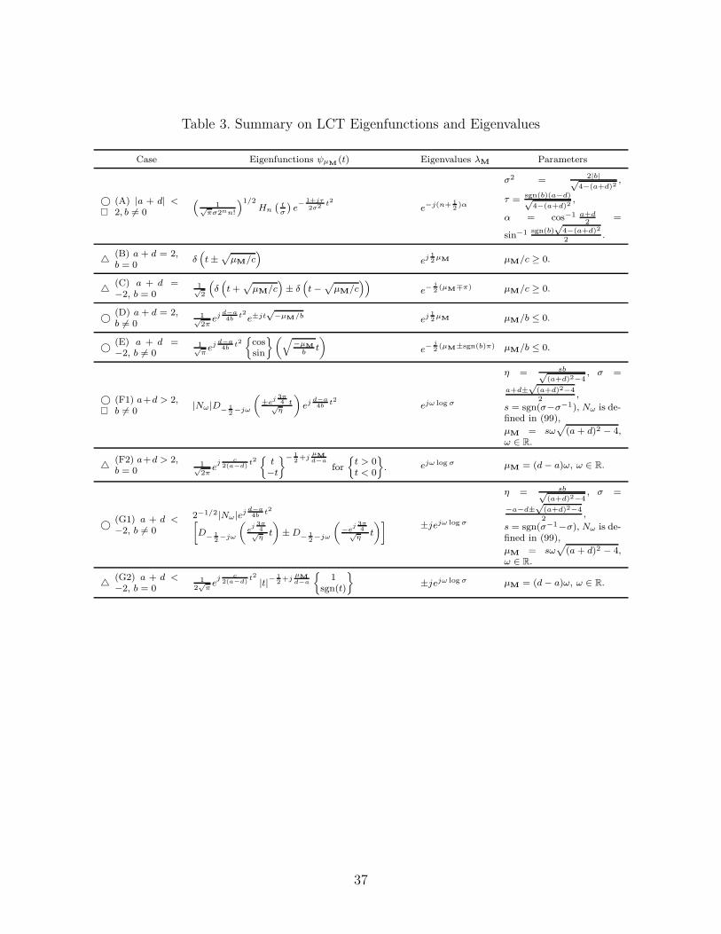
We have already studied the eigenfunctions of the LCT in detail. A summary on the eigen-
values and the eigenfunctions are made in Table 3. In this section, some symmetry about
the eigenvalues and the eigenfunctions are going to be discussed.
The eigenvalues λM in Case (B) and Case (D) are identical when they are expressed in
terms of µM. The same rule can be applied to Case (C) and Case (E). The eigenvalues for the
even/odd solution in Case (C) and Case (E) have an extra phase term ej±π/2 or ej±sgn(b)π/2,
which also exists in Case (G1) and Case (G2). The eigenvalues satisfy |λM| = 1 for each
case, as discussed in Section 4.
The eigenfunctions also have some resemblance. For b 6= 0, they all have the chirp term
ejd−a4b
t2 , which appears e−jτt2
2σ2 in Case (A) implicitly and appears in other cases explicitly.
2(a−d) and it exists in Case (F2) and Case (G2) explicitly, and in Case (B) and Case
(C) implicitly, where the chirp terms become constant phases due to the delta functions,
which can be ignored. The triangle mark △ is used to note these cases.
Case (A) and Case (F1), which are denoted by square marks�, also share some similarities.
According to (19.13.1) in [31], the parabolic cylinder functions are related to the Hermite
Gaussian functions for integer n by
Dn(ξ) = 2−n2Hn(ξ/
√2)e−
14ξ2, n = 0, 1, 2, . . . . (122)
As a result, it is interpreted that parabolic cylinder functions are generalizations
of the Hermite Gaussian functions. The parabolic cylinder functions are more general
because the parameters are complex numbers. Besides, it is noted that the parameter√η
in Case (F1) is similar to the parameter σ in Case (A), except that the terms in the square
root function are opposite. The eigenfunctions in Case (F1) also have the complex scaling
factors ±ej 3π4 in them.
Example 5.1. Here is an example to illustrate the similarity between Case (A) and Case
(F1) more closely. Consider the following two transforms
Mα =
[
cosα sinα
− sinα cosα
]
, Mβ =
[
cosh β sinh β
sinh β cosh β
]
, (123)
where α, β ∈ R, Mα corresponds the fractional Fourier transform and Mβ is the hyperbolic
subgroup [1,3]. According to Definition 3.1, The commuting operator for these two cases are
CMα = cosα(
D2t − t2
)
, CMβ= cosh β
(
D2t + t2
)
. (124)
The factors cosα and cosh β does not affect the eigenfunctions but the eigenvalues. In quan-
tum mechanics, CMα corresponds the harmonic oscillators [1,6,7,33] while CMβis the inverted
oscillators [34–37], or the repulsive oscillators [32, 38]. Our eigenfunctions in Case (F1) are
exactly the same as the existing results [32, 34].
Remark. For Case (F1), an alternative approach was proposed in [17,18]. The authors relate
Mβ with Mα by complex power of the matrices. The resultant eigenfunction for Mβ is the
Hermite Gaussian function with complex scaling factor. Our results are compared with their
results using the parabolic cylinder functions. Beginning with (21) in [18], the complex-scaled
Hermite Gaussian function can be substituted for parabolic cylinder function, (122), and the
eigenfunction is proportional to
Dn
(
t
ejπ/4σ
)
e−jτ
2σ2 t2
. (125)
23
Besides, the boundedness of this eigenfunction is checked by∣
∣
∣
∣
Dn
(
t
ejπ/4σ
)
e−jτ
2σ2 t2
∣
∣
∣
∣
=
∣
∣
∣
∣
Dn
(
t
ejπ/4σ
)∣
∣
∣
∣
=
∣
∣
∣
∣
2−n/2Hn
(
t√2ejπ/4σ
)
ejt2
4σ2
∣
∣
∣
∣
=
∣
∣
∣
∣
2−n/2Hn
(
t√2ejπ/4σ
)∣
∣
∣
∣
→ ∞ as t→ ∞. (126)
According to (125), the argument in the parabolic cylinder function, t/(ejπ4 σ) , is identical
to our result, ±ej 3π4 t/η. Besides, the additional chirp term can be simplified as ej
d−a4b
t2 . The
only difference is the index of the parabolic cylinder function. Our eigenfunction evaluates
on a straight line on the complex plane, −12− jω; however, the non-negative integer n is
required in the result of [18].
Next, the eigenvalues for both results are also compared. Our eigenvalues obey the |λM| = 1
property in each case. But, according to [18], the eigenvalues for the |a + d| > 2 case are
derived to be
λn =
eα(n−1/2) a + d > 2,
e(α−jπ)(n−1/2) a + d < −2,(127)
where α = −arccosh(∣
∣
a+d2
∣
∣
)
sgn(b). If the parameter α is positive, the eigenvalues for a+d > 2
grow rapidly as the index n approach to infinity. Due to (104), our results possess bounded
eigenfunctions and bounded eigenvalues, which are appropriate for actual computation.
The previous results in [18] and our results are both eigenfunctions of the a+ d > 2 case.
The unbounded eigenfunctions in [18] result in non-negative index n while our bounded
eigenfunctions compute the index in −12− jω. The same phenomenon sometimes occurs
in signal processing, such as the translation operator TTx(t) = x(t − T ). The exponential
function and the complex exponential function are trivial eigenfunction of TT due to
TT et = et−T =(
e−T)
et, (128)
TT ejt = ej(t−T ) =(
e−jT)
ejt. (129)
It is shown that for the translation operator TT with the same parameter T , we obtain two
distinct sets of eigenvalues and eigenfunctions. In the first set, (128), the real eigenvalue is
e−T while the real eigenfunction is et, implying the magnitude of the eigenvalue is not always
unity and the eigenfunction grows unbounded as t approaches to infinity. On the other hand,
the second set of solutions has complex eigenvalue e−jT and complex eigenfunction ejt. We
have unity magnitude of eigenvalue (∣
∣e−jT∣
∣ = 1) and bounded eigenfunction (|ejt| = 1).
It is observed that a small change on the exponential function changes the boundedness
and the resultant eigenvalue is confined in the unit circle, as indicated in (129). The previous
results in [18] is similar to (128); our eigenfunctions for |a+ d| > 2 resemble (129) more.
24
6. Application: Eigen-Decomposition of the LCT
A major application is the the discrete LCT. Apart from sampling the integral definition
(1), the LCT can be implemented by the signal expansion on the eigenspace. Our method
features perfect reconstruction when taking the inverse LCT.
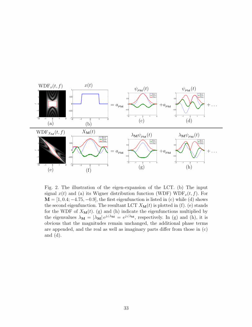
An illustrative example is given in Fig. 2. Assume that the input signal is the rectangular
function
x(t) =1√2rect
(
t
2
)
=
1/√2 |t| < 1,
0 otherwise.(130)
The signal plot is shown in Fig. 2(b). The Wigner distribution function (WDF) of x(t) is
also computed in Fig. 2(a), where the energy distribution is marked by a dashed rectangle.
Based on the complete and orthonormal eigenfunctions, the LCT can be implemented as the
following three steps:
1. Eigenfunction expansion (projection): Given x(t), the goal is to evaluate the
coefficients aµM such that
x(t) =∑
µM
aµMψµM(t). (131)
Due to the orthogonal property of the eigenfunctions, the coefficients are obtained by
taking the inner products of ψµM(t) and x(t):
aµM = 〈ψµM(t), x(t)〉 =∫ ∞
−∞ψ∗µM
(t)x(t) d t. (132)
(132) is interpreted as the eigenfunction analysis equation for the input signal x(t),
which projects x(t) onto the eigenspace to have coefficients aµM .
In the example, we select M = [1, 0.4;−4.75,−0.9] and then compute the eigenfunc-
tions based on our closed-form eigenfunctions, as shown in Fig. 2(c,d), where the real
parts, the imaginary parts, and the magnitudes are all drawn on the plots.
2. Multiply λM: Taking the LCT on both sides of (131) yields
XM(t) =∑
µM
λMaµMψµM(t), (133)
which is depicted in the bottom of Fig. 2. In this step, λMaµM is to be computed. Note
that the relationship between λM and µM was studied completely in Section 4. We can
utilize these relations for any µM.
The eigenvalues λM can be rewritten as its magnitude and phase by |λM| ej∠λM , where
∠λM indicates the phase of λM. Substituting this alternative expression into (133)
and applying Property 4 (|λM| = 1) yield aµM(
ej∠λMψµM(t))
for the summand. It is
25
evident that this step is equivalent to appending additional phase factors ej∠λM
to the eigenfunctions.
3. Eigenfunction combination: The final step is to sum up λMaµMψµM(t) over all µM,
as (133) states. In Fig. 2(g,h), λMψµM(t) is plotted. By comparing (c) and (g), it is
observed that ψµM(t) and λMψµM(t) are identical in terms of magnitude so does (d)
and (h). These observations justify Property 4, which claims |λM| = 1.
After the three-step implementation, the resultant LCT XM(t) is shown in Fig. 2(f), where
the magnitude information is plotted in solid curve. The WDF of XM(t) is also given in Fig.
2(e) for clarity. The energy distribution is now twisted into the parallelogram, which is
marked in dashed lines, by the affine transformation with parameter a, b, c and d. This illus-
trative example proves that the eigenfunctions can be applied to the LCT implementation.
The LCT via eigenfunctions has the following features other than the existing method
[39, 40]. The eigenfunctions are proved to be complete and orthogonal. Hence, taking the
inverse LCT operation LM−1 follows the three-steps implementation as long as the eigenvalues
are modified into λ−1M. Perfect recovery of the signal is ensured under our implementation
scheme.
In addition, signal expansion provides a tool for signal processing under these novel eigen-
functions. The eigenfunctions are physically meaningful in quantum mechanics and optics.
For instance, these eigenfunctions establish a orthonormal basis for studying the self-imaging
phenomenon in lossless media. These eigenfunctions also act as the wavefunctions in the
quantum system related to the LCT. In signal processing, after LCT operation, the trans-
formed output of the eigenfunction remains the same form with an additional eigenvalue
phase factor. The expansion coefficients aµM are able to be applied to signal analysis, signal
estimation, and signal modeling.
7. Conclusion
In this paper, the commuting operator CM, which commutes with LCT operator LM, was
presented. It is shown that this operator and the LCT operator share the same eigenfunctions
but have different eigenvalues. The analysis using the commuting operator unifies previous
work and enables it to be examined in an uniform manner; it also extends previous research
by finding the closed-form and bounded expression for the eigenvalues and the eigenfunctions
in the cases of |a+ d| > 2 and a + d = ±2, b 6= 0. Our work is summarized in Table 3.
In the future, the discrete LCT with perfect reconstruction property can be efficiently
calculated by the eigenfunctions. Based on the commuting operator CM, and the closed-form
expressions of λM, we can achieve discrete implementation of FrFT, scaling operation, chirp
convolution, chirp multiplication, or combinations of these operations, which are very useful
26
in digital signal processing.
Appendix A: Inner products between special functions
The inner products between some special functions throughout the paper are derived in
this appendix for clarity. The first one is 〈δ (t− α) , δ (t− β)〉. Recall that the Dirac delta
function is defined as the (inverse) Fourier transform of the constant function as follows
δ (t− α) =1
2π
∫ ∞
−∞e±jω(t−α) dω. (A1)
Taking the inner product between two deltas and applying (A1) yield
〈δ (t− α) , δ (t− β)〉 = 1
4π2
∫ ∞
−∞
∫ ∞
−∞
∫ ∞
−∞ejω1(t−α)ejω2(t−β) dω1 dω2 d t. (A2)
Integrating the variable t first gives us
〈δ (t− α) , δ (t− β)〉 = 1
2π
∫ ∞
−∞
∫ ∞
−∞e−jω1αe−jω2βδ (ω1 + ω2) dω1 dω2. (A3)
Note that the sifting property of the delta function,∫∞−∞ f(t)δ(t− t0) d t = f(t0) , can be
applied to the integrals. Letting ω1 = −ω2 and eliminating the integral with respect to ω1
lead to the following result
〈δ (t− α) , δ (t− β)〉 = 1
2π
∫ ∞
−∞ejω2(α−β) dω2 = δ (α− β) . (A4)
Next, the orthogonal property between two complex exponentials is verified. By definition,
⟨
1√2πejω1t,
1√2πejω2t
⟩
=1
2π
∫ ∞
−∞e−j(ω1−ω2)t d t. (A5)
According to (A1), we have the orthogonal property⟨
ejω1t/√2π, ejω2t/
√2π⟩
= δ (ω1 − ω2).
To prove the orthogonal property of the scale-invariant function in (83), taking the inner
product of hω(t) as defined in(80),
〈hω1(t), hω2(t)〉 =1
2π
∫ ∞
0
t−1−j(ω1−ω2) d t =1
2π
∫ ∞
0
e−j(ω1−ω2) log tt−1 d t. (A6)
Making change of variables τ = log t results in d τ = t−1 d t and
〈hω1(t), hω2(t)〉 =1
2π
∫ ∞
−∞e−j(ω1−ω2)τ d τ . (A7)
Applying the orthogonal property of the complex exponential functions to (A7), we obtain
〈hω1(t), hω2(t)〉 = δ (ω1 − ω2).
27
Appendix B: Eigenvalues of Case (C) in [14]
We examine the derivation steps (60) to (61) in [14]. Substituting (61) into (60) in [14] and
computing the terms in the brackets we have
O(−1,0,c,−1)F (φc,hC (t)) = je−jcu
2/2
[
δ
(
−u−√
4nπ
|c| + h
)
+ δ
(
−u+√
4nπ
|c| + h
)]
. (B1)
According to δ(−t) = δ(t), we obtain
O(−1,0,c,−1)F (φc,hC (t)) = je−jcu
2/2
[
δ
(
u+
√
4nπ
|c| + h
)
+ δ
(
u−√
4nπ
|c| + h
)]
. (B2)
From the sifting property of the delta functions, x(t)δ(t− t0) = x(t0)δ(t− t0), we obtain the
eigenvalues to be je−jch/2. The modified result is then exactly identical to our newly derived
result.
Acknowledgments
This work was supported by the National Science Council, R.O.C., under Contract 98-2221-
E-002-077-MY3.
References
1. H. M. Ozaktas, Z. Zalevsky, and M. A. Kutay, The Fractional Fourier Transform with
Applications in Optics and Signal Processing (Wiley, 2001).
2. S. Abe and J. T. Sheridan, “Optical operations on wave functions as the Abelian sub-
groups of the special affine Fourier transformation,” Opt. Lett. 19, 1801–1803 (1994).
3. K. B. Wolf, Integral Transforms in Science and Engineering (Plenum Publ. Corp., 1979).
4. D. F. James and G. S. Agarwal, “The generalized Fresnel transform and its application
to optics,” Optics Communications 126, 207212 (1996).
5. L. M. Bernardo, “ABCD matrix formalism of fractional Fourier optics,” Optical Eng.
35, 732–740 (1996).
6. D. J. Griffiths, Introduction to Quantum Mechanics (Pearson Prentice Hall, 2005).
7. V. Namias, “The Fractional Order Fourier Transform and its Application to Quantum
Mechanics,” J. Inst. Maths Applics 25, 241–265 (1980).
8. H. M. Ozaktas and D. Mendlovic, “Fractional Fourier optics,” J. Opt. Soc. Am. A 12,
743–751 (1995).
28
9. H. T. Yura and S. G. Hanson, “Optical beam wave propagation through complex optical
systems,” J. Opt. Soc. Am. A 4, 1931–1948 (1987).
10. D. Li, D. P. Kelly, R. Kirner and J. T. Sheridan, “Speckle orientation in paraxial optical
systems,” Appl. Opt. 51, A1–A10 (2012).
11. D. P. Kelly, J. J. Healy, B. M. Hennelly and J. T. Sheridan, “Quantifying the 2.5D
imaging performance of digital holographic systems,” J. Europ. Opt. Soc. Rap. Public.
11034 6 (2011).
12. S.-C. Pei and J.-J. Ding, “Fractional Fourier transform, Wigner distribution, and filter
design for stationary and nonstationary random processes,” IEEE Trans. Signal Process.
58, 4079–4092 (2010).
13. D. Mustard, “The fractional Fourier transform and the Wigner distribution,” J.Austral.
Math. Soc. Ser. B 38, 209–219 (1996).
14. S.-C. Pei and J.-J. Ding, “Eigenfunctions of Linear Canonical Transform,” IEEE Trans.
Signal Process. 50, 11–26 (2002).
15. J. J. Ding, “Research of fractional Fourier transform and linear canonical transform,”
Ph.D. thesis, National Taiwan University (2001).
16. G. W. Wornell, Signal Processing with Fractals: A Wavelet-Based Approach (Prentice-
Hall, 1996).
17. T. Alieva and M. J. Bastiaans, “Properties of eigenfunctions of the canonical integral
transform,” in “Proc. IEEE EURASIP Workshop on Nonlinear Signal and Image Pro-
cessing,” , vol. 2 (1999), vol. 2, pp. 585–587.
18. A. Serbes, S. Aldrmaz, and L. Durak-Ata, “Eigenfunctions of the linear canonical trans-
form,” in “Proc. of 20th Signal Processing and Communications Applications Conference
(SIU),” (2012), pp. 1–4.
19. A. Koc, H. M. Ozaktas, C. Candan, and M. A. Kutay, “Digital Computation of Linear
Canonical Transforms,” IEEE Trans. Signal Process. 56, 2383–2394 (2008).
20. J. W. Goodman, Introduction to Fourier Optics (Roberts and Company Publishers,
2005).
21. C. Candan, M. A. Kutay, and H. M. Ozaktas, “The Discrete Fractional Fourier Trans-
form,” IEEE Trans. Signal Process. 48, 1329–1337 (2000).
22. C. Candan, “On Higher Order Approximations for Hermite-Gaussian Functions and
Discrete Fractional Fourier Transforms,” IEEE Signal Process. Lett. 14, 699–702 (2007).
23. H. Kogelnik and T. Li, “Laser Beams and Resonators,” Appl. Opt. 5, 1550–1567 (1966).
24. A. E. Siegman, Lasers (University Science Books, 1986).
25. R. N. Bracewell, The Fourier Transform and Its Applications (McGrawHill, 2002), 3rd
ed.
26. L. Cohen, “The Scale Representation,” IEEE Trans. Signal Process. 41, 3275–3292
29
(1993).
27. R. G. Baraniuk and D. Jones, “Unitary equivalence: a new twist on signal processing,”
IEEE Trans. Signal Process. 43, 2269–2282 (1995).
28. R. G. Baraniuk, “Signal transform covariant to sccale changes,” Electronics Letters 29,
1675–1676 (1993).
29. M. Izzetoglu, B. Onaral, P. Chitrapu, and N. Bilgutay, “Discrete Time Processing of
Linear Scale Invariant Signals and Systems,” Proc. SPIE 4116, 110–118 (2000).
30. F. Oberhettinger, Tables of Mellin Transforms (Springer-Verlag, 1974).
31. M. Abramowitz and I. A. Stegun, eds., Handbook of Mathematical Functions With For-
mulas, Graphs, and Mathematical Tables (1965).
32. C. A. Munoz, J. Rueda-Paz, and K. B. Wolf, “Discrete repulsive oscillator wavefunc-
tions,” J. Phys. A: Math. Theor. 42 (2009).
33. L. Barker, C. Candan, T. Hakioglu, M. A. Kutay, and H. M. Ozaktas, “The discrete
harmonic oscillator, harper’s equation, and the discrete fractional fourier transform,” J.
Phys. A: Math. Gen. 33, 2209–2222 (2000).
34. E. G. Kalnins and W. Miller, “Lie theory and separation of variables. 5. The equations
iUt + Uxx = 0 and iUt + Uxxc/x2U = 0,” J. Math. Phys. 15, 1728–1737 (1974).
35. G. Barton, “Quantum Mechanics of the Inverted Oscillator Potential,” Annals of Physics
166, 322–363 (1986).
36. S. Tarzi, “The inverted harmonic oscillator: some statistical properties,” J. Phys. A:
Math. Gen. 21, 3105–3111 (1988).
37. C. Yuce, A. Kilic, and A. Coruh, “Inverted oscillator,” Phys. Scr. 74, 114–116 (2006).
38. P. G. L. Leach, “Sl(3, R) and the repulsive oscillator,” J. Phys. A: Math. Gen. 13,
1991–2000 (1980).
39. B. M. Hennelly and J. T. Sheridan, “Fast numerical algorithm for the linear canonical
transform,” J. Opt. Soc. Am. A 22, 928–937 (2005).
40. S.-C. Pei and Y.-C. Lai, “Discrete linear canonical transforms based on dilated Hermite
functions,” J. Opt. Soc. Am. A 28, 1695–1708 (2011).
30
List of Figures
1 Different cases for the eigenfunctions of the LCT, modified from [14]. . . . . 322 The illustration of the eigen-expansion of the LCT. (b) The input sig-
nal x(t) and (a) its Wigner distribution function (WDF) WDFx(t, f). ForM = [1, 0.4;−4.75,−0.9], the first eigenfunction is listed in (c) while (d)shows the second eigenfunction. The resultant LCT XM(t) is plotted in (f).(e) stands for the WDF of XM(t). (g) and (h) indicate the eigenfunctionsmultiplied by the eigenvalues λM = |λM| ej∠λM = ej∠λM , respectively. In (g)and (h), it is obvious that the magnitudes remain unchanged, the additionalphase terms are appended, and the real as well as imaginary parts differ fromthose in (c) and (d). . . . . . . . . . . . . . . . . . . . . . . . . . . . . . . . 33
31
Case (A)Case (B)Case (C)Case (D)Case (E)Case (F1)Case (F2)Case (G1)Case (G2)
|a+ d| < 2
|a+ d| = 2
b = 0
b 6= 0
a+ d = 2
a+ d = −2
a+ d = 2
a+ d = −2
a+ d > 2
a+ d < −2
b 6= 0
b = 0
b 6= 0
b = 0
Fig. 1. Different cases for the eigenfunctions of the LCT, modified from [14].
32
WDFx(t, f)
t
f
−2 −1 0 1 2−2
−1
0
1
2
(a)
x(t)
−2 −1 0 1 2−1
−0.5
0
0.5
1
t
(b)
= aµM
ψµM(t)
−2 −1 0 1 2−1
−0.5
0
0.5
1
t
RealImag.Mag.
(c)
+aµM
ψµM(t)
−2 −1 0 1 2−1
−0.5
0
0.5
1
t
RealImag.Mag.
(d)
+ . . .
WDFXM(t, f)
t
f
−2 −1 0 1 2−2
−1
0
1
2
(e)
XM(t)
−2 −1 0 1 2−1
−0.5
0
0.5
1
t
RealImag.Mag.
(f)
= aµM
λMψµM(t)
−2 −1 0 1 2−1
−0.5
0
0.5
1
t
RealImag.Mag.
(g)
+aµM
λMψµM(t)
−2 −1 0 1 2−1
−0.5
0
0.5
1
t
RealImag.Mag.
(h)
+ . . .
Fig. 2. The illustration of the eigen-expansion of the LCT. (b) The inputsignal x(t) and (a) its Wigner distribution function (WDF) WDFx(t, f). ForM = [1, 0.4;−4.75,−0.9], the first eigenfunction is listed in (c) while (d) showsthe second eigenfunction. The resultant LCT XM(t) is plotted in (f). (e) standsfor the WDF of XM(t). (g) and (h) indicate the eigenfunctions multiplied bythe eigenvalues λM = |λM| ej∠λM = ej∠λM, respectively. In (g) and (h), it isobvious that the magnitudes remain unchanged, the additional phase termsare appended, and the real as well as imaginary parts differ from those in (c)and (d).
33
List of Tables
1 Summary on the eigenfunctions and the eigenvalues [14] . . . . . . . . . . . . 352 The commuting operators for some special cases of the LCT. . . . . . . . . . 363 Summary on LCT Eigenfunctions and Eigenvalues . . . . . . . . . . . . . . . 37
34
Table 1. Summary on the eigenfunctions and the eigenvalues [14]
Case Eigenfunctions ψ(t) Eigenvalues Parameters
(A) |a+ d| < 2(
1√πσ2nn!
)1/2Hn
(
tσ
)
e− 1+jτ
2σ2 t2e−j(n+ 1
2 )α
σ2 = 2|b|√4−(a+d)2
,
τ =sgn(b)(a−d)√
4−(a+d)2,
α = cos−1 a+d2
=
sin−1 sgn(b)√
4−(a+d)2
2.
(B) a + d = 2,b = 0
E− 12
(
∑∞n=0Anδ
(
t −√
4nπ|c| + h
)
+∑∞
m=0Bmδ(
t+√
4mπ|c| + h
)) ejch/20 ≤ h ≤ 4π
|c| , E =∑∞
n=0
(
|An|2 + |Bn|2)
(C) a+d = −2,b = 0
The same case as B, except for An = ±Bn for alln.
±je−jch/2 Explained in (B1) and (B2)
(D) a + d = 2,b 6= 0
√
1j2πρ
ejd−a4b
t2∫∞−∞ e
j(t−ξ)2
2ρ g(ξ) d ξ e−jbh/2
g(t) =√
12πS
[
∑∞n=0 Cne
jt√
4nπ|b|
+h
+∑∞
m=0Dme−jt
√
4mπ|b|
+h]
,
0 ≤ h < 4π|b| , S =
∑∞n=0
(
|Cn|2 + |Dn|2)
(E) a+d = −2,b 6= 0
The same as case D, except for Cn = ±Dn. ±je−jbh/2
(F) a + d > 2 1√j2πη
ejτ2t2
∫∞−∞ e
j2η
(t−ξ)2h(ξ) d ξ λ
√σh(σt) = λh(t),
τ = −2sc
s(d−a)+√
(a+d)2−4, η =
sb√(a+d)2−4
,
σ =a+d±
√(a+d)2−4
2, s =
sgn(σ − σ−1).
(G) a+ d < −2The same as case F, except for h(t) = ±h(−t)must be satisfied and s = sgn(σ−1 − σ)
λ
35
Table 2. The commuting operators for some special cases of the LCT.
Operation Commuting operator
Scaling tDt +DttChirp convolution D2
t
Chirp multiplication t2
(fractional) Fourier transform D2t − t2
hyperbolic D2t + t2
36
Table 3. Summary on LCT Eigenfunctions and Eigenvalues
Case Eigenfunctions ψµM(t) Eigenvalues λM Parameters