Dimensional Analysis and Its Applications in Statistics

mss # 1739.tex; art. # 01; 46(3)

Dimensional Analysis and Its

Applications in Statistics

WEIJIE SHEN

The Pennsylvania State University, University Park, PA 16802, USA

TIM DAVIS

We Predict Ltd., Technium 1, Kings Road, Swansea, SA1 8PH, UK

DENNIS K. J. LIN

The Pennsylvania State University, University Park, PA 16802, USA

CHRISTOPHER J. NACHTSHEIM

University of Minnesota, Minneapolis, MN 55455, USA

Dimensional analysis (DA) is a well-developed, widely-employed methodology in the physical and en-gineering sciences. The application of dimensional analysis in statistics leads to three advantages: (1) thereduction of the number of potential causal factors that we need to consider, (2) the analytical insightsinto the relations among variables that it generates, and (3) the scalability of results. The formalization ofthe dimensional-analysis method in statistical design and analysis gives a clear view of its generality andoverlooked significance. In this paper, we first provide general procedures for dimensional analysis prior tostatistical design and analysis. We illustrate the use of dimensional analysis with three practical examples.In the first example, we demonstrate the basic dimensional-analysis process in connection with a studyof factors that a↵ect vehicle stopping distance. The second example integrates dimensional analysis intothe regression analysis of the pine tree data. In our third example, we show how dimensional analysiscan be used to develop a superior experimental design for the well-known paper helicopter experiment.In the regression example and in the paper helicopter experiment, we compare results obtained via thedimensional-analysis approach to those obtained via conventional approaches. From those, we demonstratethe general properties of dimensional analysis from a statistical perspective and recommend its usage basedon its favorable performance.

Key Words: Buckingham’s ⇧ Theorem; Design of Experiment; Dimensions; Statistical Analysis.

1. Introduction

DIMENSIONAL ANALYSIS (DA) is a well-establishedmethod in physics (see Sonin (2001), Szirtes

(2007)). Bridgman (1931) stated that “The principaluse of dimensional analysis is to deduce from a studyof the dimensions of the variables in any physical sys-tem certain limitations on the form of any possible

Mr. Shen is a Doctoral Student in the Department of Statis-

tics, Pennsylvania State University. His email address is weijie

[email protected].

Dr. Davis is the Director of Timdavis Consulting Ltd.,

Chief Technical O�cer at We Predict Ltd., and Professor at

the University of Warwick. His email address is tim@timdavis

.co.uk.

Dr. Lin is a Distinguished Professor of Statistics and Sup-

ply Chain in the Department of Statistics, Pennsylvania State

University. His email address is [email protected].

Dr. Nachtsheim is a Professor, the Frank A. Donaldson

Chair of Operations Management, and Chair of the Supply

Chain and Operations Department in the Carlson School of

Management, University of Minnesota. His email address is

[email protected].

Vol. 46, No. 3, July 2014 185 www.asq.org

mss # 1739.tex; art. # 01; 46(3)

186 WEIJIE SHEN ET AL.

relationship between those variables. The method isof great generality and mathematical simplicity”. Itis mainly used to find the relations among physicalquantities in complicated physical systems by theirdimensions. A variety of literature has applied di-mensional analysis in various fields. See Asmussenand Heebooll-Nielsen (1955), Islam and Lye (2009),and Stahl (1962), for examples. Through these anal-yses, some simple rules among those quantities canbe extracted. As a dimension-reduction and feature-extraction methodology, dimensional analysis couldbe of great use to the field of statistics. This a pri-ori analysis gives us a conceptual and analytical viewof the problem we are dealing with, thereby provid-ing guidance in both the design and analysis steps.Furthermore, the physical origin of dimensional anal-ysis improves the interpretability of the final results,which is particularly desirable to the fields of physicsand engineering.

Unfortunately, statisticians seem to have over-looked the advantages of dimensional analysis.Finney (1977) commented that “I am surprised bythe lack of attention given to dimensions as a checkon the theory and practice of statistics. The basicideas, readily appreciated, should form part of thestock-in-trade of every statistician”. In this paper,we focus on building functional relationships betweeninputs and outputs. We will first introduce the basicconcept and general procedure of dimensional anal-ysis. Illustrated by two examples, the pine tree andpaper helicopter, we show how to apply dimensionalanalysis in real problems and also compare the resultswith classic approaches. We summarize the proper-ties and discuss the advantages of dimensional anal-ysis in the statistical context.

The rest of the paper is organized as follows. Inthe Section 2, we introduce the definitions and gen-eral procedures of dimensional analysis with an il-lustrative example. In Section 3, we use dimensionalanalysis for data analysis and show its generality andimportance. In Section 4, dimensional analysis is ap-plied to design of experiments. The last two sectionssummarize general properties, followed by some con-cluding remarks and prospective research.

2. Definitions of Dimensional Analysisand General Procedure with

Illustrative Example2.1. Physical Dimensions

In mathematics, dimension typically refers to thenumber of coordinates required to define points in

abstract spaces, whereas in statistics, dimension typ-ically refers to the number of variables in a designproblem or a data set. However, physical dimen-sions refer to the measurement systems to charac-terize certain objects. Each physical dimension hasseveral empirical scales of the measurements andthey are called “units”. Ignoring nuclear e↵ects suchas isospin, charm, and strangeness, there are sevenfundamental physical dimensions: namely, mass M,length L, time T, temperature ⇥, electric current I(or charge Q), amount of substance mol, and lumi-nous intensity Iv. The corresponding units, definedby SI (International System of Units), are kilogram,meter, second, kelvin, ampere, mole, and candela, re-spectively. All other physical quantities are combina-tions of these fundamental quantities and their unitsare combinations of the units of the correspondingfundamental quantities, combined in the same way.For example, speed has the dimension of length pertime, for which the SI unit is meters per second.

2.2. Background of Dimensional Analysis

Physical quantities cannot be constructed unre-strictedly. For example, it makes no sense to add“length” to “mass” due to the natural constraints inthe physical quantities. The main constraint is that“a physical law must be independent of the unitsused to measure the physical quantities”. This wasfirst proposed by Joseph Fourier in the 19th cen-tury (see Mason (1962)). This principle has beenformalized in two important theorems, Bucking-ham’s ⇧-theorem (Buckingham (1914, 1915a,b)) andBridgman’s principle of absolute significance of rela-tive magnitude (Bridgman, 1931). Buckingham’s ⇧-theorem shows that physical equations must be di-mensionally homogeneous. In other words, any mean-ingful equations (and inequalities) must have thesame dimensions in both the left and right sides.Bridgman’s principle of absolute significance of rela-tive magnitude shows that such formulae should be inthe power-law form. Basically, Bridgman’s principleallows us to transform physical quantities properly,especially into dimensionless forms. The method ofusing dimensionless quantities and Buckingham’s ⇧-theorem to remove such constraints is called dimen-sional analysis. Next, we introduce Buckingham’s ⇧-theorem and how to use it in practice.

2.3. General Procedure

We recommend applying dimensional analysis be-fore statistical analysis to give a general view of theproblems and the variables involved. From the physi-

Journal of Quality Technology Vol. 46, No. 3, July 2014

mss # 1739.tex; art. # 01; 46(3)

DIMENSIONAL ANALYSIS AND ITS APPLICATIONS IN STATISTICS 187

cal perspective, procedures can be found in Taylor etal. (2007) and others. From the statistical perspec-tive, the general procedure of dimensional analysiscan be specified as follows:

Step 1. Determine the input and output variablesand their dimensions, respectively.

Step 2. Determine the basis quantities.Step 3. Transform input and output variables into

dimensionless quantities by using basisquantities in step 2.

Step 4. Re-express the model functions via trans-formed variables in step 3.

Step 1

Determine the input and output variables ofthe system we consider. Denote input variables asQ1, . . . , Qp and the output variable (response) as Q0.The conventional model will be Q0 = f(Q1, . . . , Qp),where f is the model function to be estimated. Notethat, in dimensional analysis, Qi may include rel-evant physical constants with dimensions, such asgravitational constant = 6.67300⇥10�11m3kg�1s�2.The units are often standardized to avoid dimension-less multiplicative constants. But standardization isnot always necessary because these constants arecombined into unknown functional relationships. Af-ter checking the physical meaning of all the variableswe consider, we determine the relevant fundamen-tal physical quantities in the system of the seven SIunits as shown in the previous section: denote themas q1, . . . , q7. Further denote the dimensions of Qi as[Qi] and qj as [qj ] for i = 0, 1, . . . , p, j = 1, . . . , 7. Weexpress the dimensions of Q0, Q1, . . . , Qp in termsof [q1], . . . , [q7] as [Qi] = [q1]ri1 · · · [q7]ri7 , for someproper choices of {rij} with i = 0, 1, . . . , p, j =1, . . . , 7.

Step 2

Determine the basis quantities. The basis quanti-ties constitute a subset of the inputs. We reorder anddenote them as Q1, . . . , Qt, where t 7 as discussedabove and t p. The basis quantities should satisfytwo conditions: (1) “Representativity”: the dimen-sions of any other quantities, [Q0], [Qt+1], . . . , [Qp]can be expressed by the combinations of the dimen-sions of the basis quantities, [Q1], . . . , [Qt]. The com-binations take the form of power law. (2) “Indepen-dence”: the dimension of any basis quantities cannotbe expressed by the combinations of the dimensionsof other basis quantities. Furthermore, assume that[Q0] can be expressed by the combinations of [Qi],

i = 1, . . . , p. If not, dimensional homogeneity is vio-lated. This assumption leads to the existence of thebasis quantities but they are not unique. However,the number of basis quantities is a fixed constant.The concept of basis in linear algebra is a very goodanalogy to the concept of basis quantities.

Step 3

Transform input and output variables into di-mensionless quantities by using basis quantities. Wemainly transform variables that are not basis quan-tities, i.e., Q0, Qt+1, . . . , Qp, based on Buckingham’s⇧-theorem. Due to the two properties of basis quan-tities in step 2, we can have [Qi] = [Q1]di1 · · ·[Qt]dit , i = 0, t + 1, t + 2, . . . , p. Consequently, thetransformed dimensionless quantities are ⇧i = Qi ·Q�di1

1 · · ·Q�ditt , i = 0, t + 1, t + 2, . . . , p, because

[⇧i] = [QiQ�di11 · · ·Q�dit

t ]= [Q1]di1 · · · [Qt]dit [Q1]�di1 · · · [Qt]�dit

= 1.

Step 4

Re-express the response functions. Before using di-mensional analysis, we have Q0 =f(Q1, . . . , Qt, Qt+1,. . . , Qp). Using ⇧i instead of Qi, we have the follow-ing expression:

⇧0Qd011 · · ·Qd0t

t

= f(Q1, . . . , Qt,⇧t+1Qdt+1,11 · · ·Qdt+1,t

t , . . . ,

⇧pQdp11 · · ·Qdpt

t )

and

⇧0 = Q�d011 · · ·Q�d0t

t

⇥ f(Q1, . . . , Qt,⇧t+1Qdt+1,11 · · ·Qdt+1,t

t , . . . ,

⇧pQdp11 · · ·Qdpt

t ),

where f is the function we hope to estimate. So wecan rewrite it as

⇧0 = g(Q1, . . . , Qt,⇧t+1, . . . ,⇧p),

where ⇧i, i = 0, t + 1, . . . , p are dimensionless andQ1, . . . , Qt are “independent”. Buckingham’s theo-rem indicates that Q1, . . . , Qt should not be in theformula. This implies ⇧0 = g(⇧t+1, . . . ,⇧p) to be thefinal model.

2.4. Example: Vehicle Stopping Distance

Here we use the vehicle stopping distance exam-ple to illustrate the general procedure. In the exper-iment, we estimate the stopping distance for cars, a

Vol. 46, No. 3, July 2014 www.asq.org

mss # 1739.tex; art. # 01; 46(3)


key indication of their safety. Assume that the driverrequires a certain amount of time for reaction to anemergency and that the wheels are not locked whenbraking. We show the dimensional analysis below us-ing the procedure described in the previous section.

Step 1. Identify input and output variables and theirdimensions as follows:

Q0 = D : vehicle stopping distance [D] = L.

Q1 = v : velocity of the vehicle [v] = LT�1.

Q2 = ⌧ : thinking time [⌧ ] = T.

Q3 = m : mass of the car [m] = M.

Q4 = F : braking force on the brake discs[F ] = MLT�2.

Q5 = µ : friction coe�cient of brakes [µ] = 1.

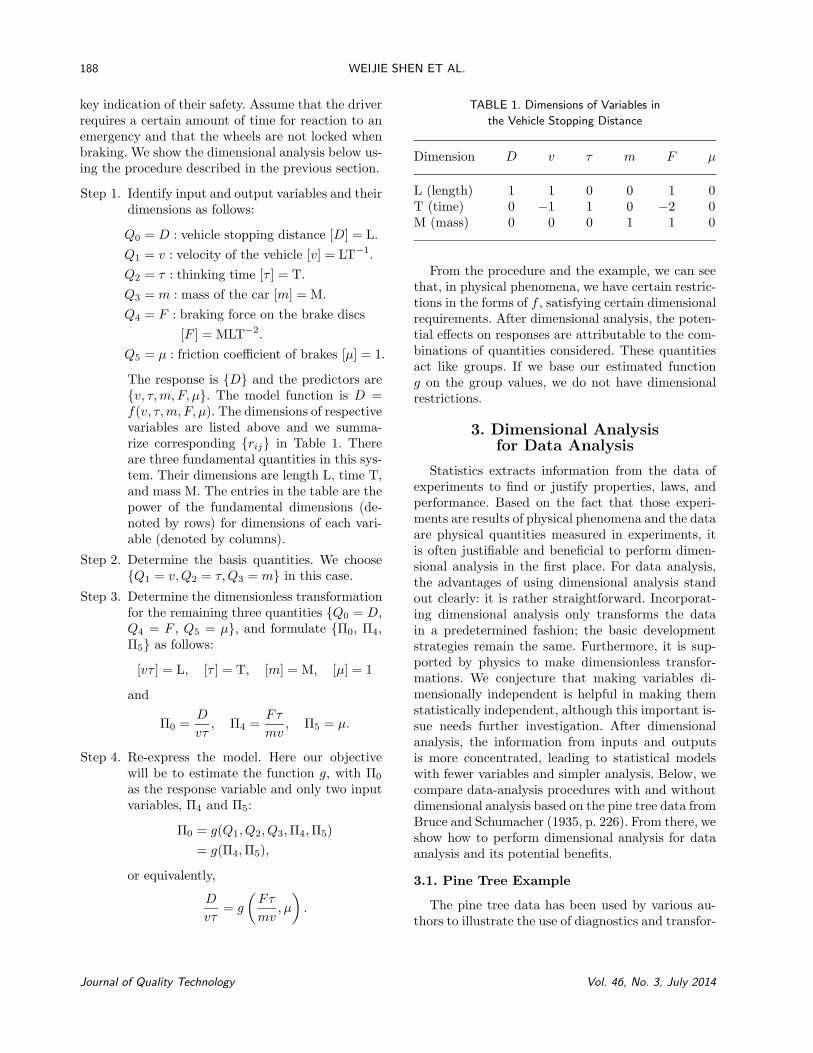
The response is {D} and the predictors are{v, ⌧,m, F, µ}. The model function is D =f(v, ⌧,m, F, µ). The dimensions of respectivevariables are listed above and we summa-rize corresponding {rij} in Table 1. Thereare three fundamental quantities in this sys-tem. Their dimensions are length L, time T,and mass M. The entries in the table are thepower of the fundamental dimensions (de-noted by rows) for dimensions of each vari-able (denoted by columns).

Step 2. Determine the basis quantities. We choose{Q1 = v,Q2 = ⌧, Q3 = m} in this case.

Step 3. Determine the dimensionless transformationfor the remaining three quantities {Q0 = D,Q4 = F , Q5 = µ}, and formulate {⇧0, ⇧4,⇧5} as follows:

[v⌧ ] = L, [⌧ ] = T, [m] = M, [µ] = 1

and

⇧0 =D

v⌧, ⇧4 =

F ⌧

mv, ⇧5 = µ.

Step 4. Re-express the model. Here our objectivewill be to estimate the function g, with ⇧0

as the response variable and only two inputvariables, ⇧4 and ⇧5:

⇧0 = g(Q1, Q2, Q3,⇧4,⇧5)= g(⇧4,⇧5),

or equivalently,

D

v⌧= g

✓F ⌧

mv, µ

◆.

TABLE 1. Dimensions of Variables inthe Vehicle Stopping Distance

Dimension D v ⌧ m F µ

L (length) 1 1 0 0 1 0T (time) 0 �1 1 0 �2 0M (mass) 0 0 0 1 1 0

From the procedure and the example, we can seethat, in physical phenomena, we have certain restric-tions in the forms of f , satisfying certain dimensionalrequirements. After dimensional analysis, the poten-tial e↵ects on responses are attributable to the com-binations of quantities considered. These quantitiesact like groups. If we base our estimated functiong on the group values, we do not have dimensionalrestrictions.

3. Dimensional Analysisfor Data Analysis

Statistics extracts information from the data ofexperiments to find or justify properties, laws, andperformance. Based on the fact that those experi-ments are results of physical phenomena and the dataare physical quantities measured in experiments, itis often justifiable and beneficial to perform dimen-sional analysis in the first place. For data analysis,the advantages of using dimensional analysis standout clearly: it is rather straightforward. Incorporat-ing dimensional analysis only transforms the datain a predetermined fashion; the basic developmentstrategies remain the same. Furthermore, it is sup-ported by physics to make dimensionless transfor-mations. We conjecture that making variables di-mensionally independent is helpful in making themstatistically independent, although this important is-sue needs further investigation. After dimensionalanalysis, the information from inputs and outputsis more concentrated, leading to statistical modelswith fewer variables and simpler analysis. Below, wecompare data-analysis procedures with and withoutdimensional analysis based on the pine tree data fromBruce and Schumacher (1935, p. 226). From there, weshow how to perform dimensional analysis for dataanalysis and its potential benefits.

3.1. Pine Tree Example

The pine tree data has been used by various au-thors to illustrate the use of diagnostics and transfor-


mss # 1739.tex; art. # 01; 46(3)


mation methods in linear regression (see, e.g., Atkin-son (1994)). The data arise from the measurements of70 shortleaf pine trees. Three measurements of inter-est here are d, the diameter of the tree in feet takenat “breast height” above the ground; h, the height ofthe tree in feet; and v, the volume in cubic feet. Theobjective of the analysis is to establish a relationshipbetween the volume v and the variables d and h. Inother words, we hope to predict the volume of a treefrom its known diameter and height. The completedata set is given in the Appendix.

3.2. Regression Method Without DimensionalAnalysis for Pine Tree Data Set

The conventional linear regression assumes that

vi = ↵ + �1di + �2hi + ✏i, (1)

with ✏i ⇠ i.i.d. N(0,�2). It gives us the following es-timated function with standard errors of estimationsin subscripts:

v̂ = �45.3(5.0) + 77.2(5.9)d + 0.12(0.11)h, (2)

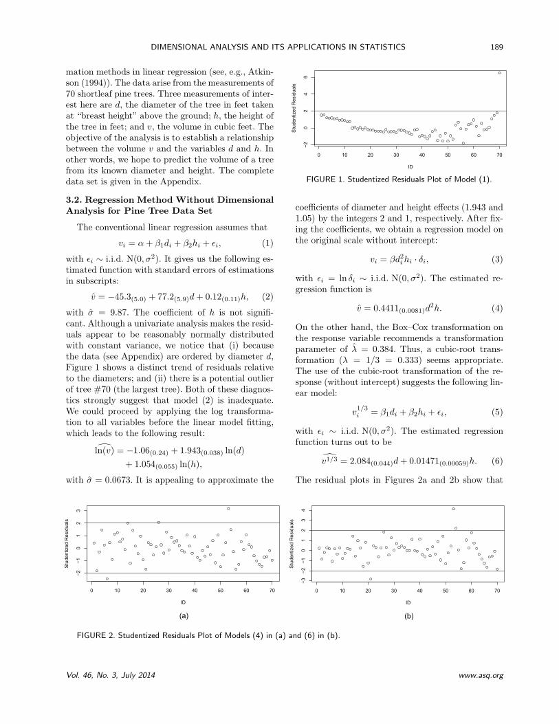
with �̂ = 9.87. The coe�cient of h is not signifi-cant. Although a univariate analysis makes the resid-uals appear to be reasonably normally distributedwith constant variance, we notice that (i) becausethe data (see Appendix) are ordered by diameter d,Figure 1 shows a distinct trend of residuals relativeto the diameters; and (ii) there is a potential outlierof tree #70 (the largest tree). Both of these diagnos-tics strongly suggest that model (2) is inadequate.We could proceed by applying the log transforma-tion to all variables before the linear model fitting,which leads to the following result:

dln(v) = �1.06(0.24) + 1.943(0.038) ln(d)+ 1.054(0.055) ln(h),

with �̂ = 0.0673. It is appealing to approximate the

FIGURE 1. Studentized Residuals Plot of Model (1).

coe�cients of diameter and height e↵ects (1.943 and1.05) by the integers 2 and 1, respectively. After fix-ing the coe�cients, we obtain a regression model onthe original scale without intercept:

vi = �d2i hi · �i, (3)

with ✏i = ln �i ⇠ i.i.d. N(0,�2). The estimated re-gression function is

v̂ = 0.4411(0.0081)d2h. (4)

On the other hand, the Box–Cox transformation onthe response variable recommends a transformationparameter of �̂ = 0.384. Thus, a cubic-root trans-formation (� = 1/3 = 0.333) seems appropriate.The use of the cubic-root transformation of the re-sponse (without intercept) suggests the following lin-ear model:

v1/3i = �1di + �2hi + ✏i, (5)

with ✏i ⇠ i.i.d. N(0,�2). The estimated regressionfunction turns out to be

dv1/3 = 2.084(0.044)d + 0.01471(0.00059)h. (6)

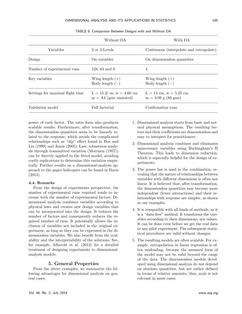
The residual plots in Figures 2a and 2b show that

FIGURE 2. Studentized Residuals Plot of Models (4) in (a) and (6) in (b).


mss # 1739.tex; art. # 01; 46(3)


both log transformation and Box–Cox transforma-tion have fixed the problems highlighted in Figure 1.Note that tree #53 deserves special attention, butwill not be further studied in this paper.

The preceding analyses were, of course, conductedwithout using dimensional analysis. However, a fur-ther look at equations (4) and (6) reveals that bothmethods provide dimensionally homogeneous solu-tions to the prediction problem. The physical dimen-sions are coherent in the equations. Model (4) has thedimension of cubic length on both sides while model(6) has the dimension of length on both sides.

3.3. Regression Method with DimensionalAnalysis for Pine Tree Data Set

Following the general procedure that we proposedin Section 2.3, the dimensional analysis can be im-plemented as below. A similar approach was outlinedin Vignaux and Scott (1999).

1. Our objective is to predict the output volumev as a function of diameter d and height h: v =f(d, h). We determine the physical dimensionsof these quantities in Table 2. The dimensionof v is cubic length L3 with unit feet3. Bothdimensions of d and h are length L with unitsin feet.

2. Because the only dimension involved is length,let h be the basis quantity.

3. Transform other quantities into dimensionlessforms,

⇧v =v

h3and ⇧d =

d

h.

4. By Buckingham’s ⇧-theorem, the predictedfunction should be ⇧v = g(⇧d), or equivalently,

v

h3= g

✓d

h

◆.

Suppose⇧v = g(⇧d), and we choose g(⇧d) = k⇧�d .

After taking the logarithm of both sides, we obtainthe linear model,

ln(⇧v,i) = ln(k) + � ln(⇧d,i) + ✏i,

with ✏i ⇠ N(0,�2). The estimated regression func-tion is

ˆln(⇧v) = �1.07(0.16) + 1.942(0.036) ln(⇧d) (7)

Alternatively, we might prefer that ⇧v = g(⇧d) =k⇧2

d. Figure 3 shows the data and linear fits in termsof ⇧v and ⇧2

d. In fact, fitting a linear model yields

TABLE 2. Dimensions of Quantities in Pine Tree Data Set

Name Quantity Dimension Unit

Volume v L3 feet3Diameter d L feetHeight h L feet

⇧̂v = 0.4363(0.0036)⇧2d,

i.e.,v̂ = 0.4363(0.0036)d

2h. (8)

The result is similar to the log-transformed model (4)and it also accommodates the problematic 70th case.The di↵erences in parameter estimates can be at-tributed to di↵erences in associated error structures.

In summary, certain assumptions regarding theform of the function g will give corresponding pa-rameterizations and results. If ⇧v = k⇧�

d , then v =kd�h3�� . If ⇧v = (A⇧d +B)3, then v1/3 = Ad+Bh.These are exactly the two models previously obtainedin equations (4) and (6). The dimensionally homoge-neous results we derived from regression analyses aremerely special cases of choosing di↵erent functionsg after dimensional analyses. The procedure ensuresthat the results are dimensionally homogeneous andintuitively interpretable, while leaving choice of thefunction g to the investigator, as informed by thedata. It gives us a guide of how to model in an ef-ficient and parsimonious way based on the physicallaws.

FIGURE 3. Plot of Pine Tree Data Set in Terms of Di-mensionless Variables.


mss # 1739.tex; art. # 01; 46(3)


In contrast with the analysis and discussion ofthe same dataset by Atkinson (1994), dimensionalanalysis points to an “automatic” transformationof the data, without prior assumption of the coneshape, and posterior diagnosis of “transform bothsides model” as Atkinson (1994) did. Moreover, be-cause the dimensional analysis of each tree is thesame, there is less need to worry about individualtrees influencing the choice of transformation, andhence regression methods such as constructed vari-able plots, which Atkinson (1994) used, are no longernecessary.

3.4. Remarks

From an analytic perspective, dimensional analy-sis o↵ers several advantages relative to the conven-tional procedures. First, it decreases the number ofvariables, which may lead to a simpler model. Sec-ond, physical independence may establish a simplerstatistical relationship. Third, it gives more sensi-ble interpretations by having dimensionless variablesand coe�cients. Physicists and engineers often fa-vor dimensionless coe�cients as indices for describ-ing systems. Fourth, dimensional analysis producesscalable results, which is necessary for extrapolation,although the scalability depends on a good choiceof the model. This is attributed to the ratio formof dimensionless variables that is invariant to scalechanges. Often, extrapolating in the original scale re-sults in values interpolating in the transformed scale.Fifth, it captures the inherent nonlinear relationshipbetween physical quantities.

From a practical perspective, dimensional anal-ysis is applicable when modeling physical relation-ships. It is a straightforward method before collect-ing data and modeling. It fits all kinds of data struc-tures and modeling requirements. Furthermore, di-mensional analysis does not lose generality whentransforming the data. As shown above, it does notconstrain the forms of estimating functions for di-mensionally homogeneous solutions. Due to its an-alytical nature, the proposed procedure is easy toimplement.

4. Dimensional Analysis forthe Design of Experiments

Dimensional analysis can also serve as a guid-ance in the design of experiments. For the designof experiments, incorporating dimensional analysiscan significantly improve e�ciency by reducing thenumber of experimental variables. In this section, wedemonstrate the use of dimensional analysis in thedesign and analysis of the popular paper helicopterexperiment. We also compare the results to those ob-tained using the conventional design of experimentsapproaches.

4.1. The Paper Helicopter Experiment

The paper helicopter experiment is a widely usedteaching device for the design of experiments. Theobjective is to predict the “flight time” performancefor a particular configuration of the helicopter dimen-sions in Figure 4. Upon its launch, twin blades spin

FIGURE 4. Paper Helicopter Illustration.


mss # 1739.tex; art. # 01; 46(3)


around the central ballast shaft to provide lift as itdescends. It can be easily constructed from a sheetof paper using only scissors and tape. As displayedin Figure 4, the upper part of the model consists oftwo wings (or rotors). The central part is the bodyand the lower part is the tail folded into the ballast.The length and width of each part can be varied toachieve di↵ering levels of performance. We wish topredict the flight time for a given configuration. Theusual design factors include the rotor radius (r), therotor width (w), the tail length (l), the tail width(d), paper clip (p), and the tape (t).

4.2. Conventional Design of the PaperHelicopter Experiment Without UsingDimensional Analysis

Johnson et al. (2006a, b) studied experimental de-sign on the paper helicopter as part of a Six SigmaBlack Belt project. They considered a Resolution VIIdesign with seven two-level factors in a half fraction,with two replicates. This led to 27�1⇥2 (= 128) runsin total. They provided a step-by-step routine to de-sign experiments and maximize the flight time. Boxand Liu (1999) and Box (1999) discussed the use ofsequential design in the paper helicopter experiment.First, they conducted a two-level Resolution IV frac-tional factorial design with eight factors in four repli-cates, i.e., 28-4

IV ⇥4, for a total of 64 runs. In the second

setting, they designed a full-factorial experiment in-volving four important factors. Two key lessons fromtheir work, among others, are (1) with the help ofresponse surface and steepest ascent, sequential de-signs search for an optimum point e↵ectively and ef-ficiently and (2) minimum variance or dispersion offlight time is included in addition to longest flighttime to enrich the meaning of optimum. Annis (2005)derived the aerodynamics of this flying object in arigorous physical sense before designing the experi-ment. He presented a physical model of flight time interms of the length and width of wing and body. Heemployed two three-level factors in a single replicateof a 3⇥ 3 factorial design for wing length and widthand employed response surface methods to identifythe optimal operating condition. The use of physicsto identify promising factors in advance turned outto be extremely advantageous.

Table 3 summarizes the results of the above threepapers, including Johnson et al., (2006a,b), Box andLiu (1999), and Annis (2005). The directions ofrespective e↵ects are provided in the parentheses.Three variables are included in all of the three ex-periments; namely, body length, body width, andwing length. Additionally, Johnson et al. (2006a, b)considered (i) paper type, (ii) whether or not tap-ing body and wing, and (iii) whether or not clippingin the bottom. They also examined the two-way in-

TABLE 3. Summary of Literature on Paper Helicopter

Johnson et al. (2006a,b) Box and Liu (1999) Annis (2005)

Input variables Body length (�) Body length (�) Body length (�)*Body width (�) Body width (�) Body width (�)*Wing length (+) Wing length (+) Wing length (+)Paper type (�) Paper type (�) Wing width (dip)Taped body (�) Taped body (�)Taped wing (�) Taped wing (�)Clip (�) Clip (�)Interactions Fold (�)

Design 27-1VII ⇥ 2 = 128 28-4

IV ⇥ 4 = 64 32 = 9

Feature Interactions Sequential learning Physical insight

Significant variables Body length (�) Body length (�) Body length (�)Body width (�) Body width (�) Body width (�)Wing length (+) Wing length (+) Wing length (+)

*Not a design factor.


mss # 1739.tex; art. # 01; 46(3)


teractions between the variables of interest. Box andLiu (1999) considered whether to fold the paper anduse an additional 50 runs to search for the optimum.Their second design included a full-factorial exper-iment on both the length and width of both bodyand wing. Annis (2005) took wing width as an ad-ditional variable and chose wing length and widthto be experimental variables and considered e↵ectsof body length and width as given by the physicalformula. The “dip” e↵ect of wing width means therelationship is not monotone. In general, the signs inthe parentheses indicate the e↵ects of each variableon the flight time. For example, wing length has apositive e↵ect on the flight time, meaning that theflight time will increase if wing length is increased.All the above studies concluded that the wing lengthis the most important factor for determining flighttime, with factors a↵ecting helicopter mass also be-ing important.

4.3. Design of the Paper HelicopterExperiment Using Dimensional Analysis

The physics of falling objects in a gravitationalfield follows the following assumptions: (1) the flighttime (T ) is determined by the launch height (H) andaverage velocity (v), i.e., T = H/v; (2) the falling ob-ject reaches terminal velocity quickly after dropped,when the drag force of the air becomes equal to theforce of gravity; (3) the drag force depends on thedensity of dry air (⇢ = 1.20412 kgm�1 at sea level at20�C), drag coe�cient (cd, dimensionless) and theshape of the helicopter (rotor radius r and rotorwidth w, or their combinations, such as ratio r/w andarea rw); (4) the weight of the helicopter depends onthe mass (m) and acceleration due to gravity (g = 9.8ms�2).

Suppose the flight time follows the model below,

T = f1(m, g, r, cd, ⇢,H).

Because cd is dimensionless and T = H/v, the ex-pression can be represented as

v = f2(m, g, ⇢, r). (9)

Next, we apply dimensional analysis step-by-step.

Step 1. Table 4 displays the dimensions and unitsof the variables. We have three fundamentaldimensions, length L, time T, and mass M.

Step 2. Variables r, ⇢, and g are chosen as the basequantities.

Step 3. From Buckingham’s ⇧ theorem, we can re-duce the number of variables from five to

two. Following Gearhart (2004), we definethe two dimensionless variables as �v =vra⇢bgc and m = mrd⇢egf . Dimensions of�v and m are, thus, as follows:

[�v] = (LT�1)(L)a(ML�3)b(LT�2)c

= L1+a�3b+cMbT�1�2c

[ m] = (ML)d(ML�3)e(LT�2)f

= Ld�3e+fM1+eT�2f .

We enforce nondimensionality and solve thetwo sets of linear equations,

1 + a� 3b + c = 0b = 0

�1� 2c = 0

and

d� 3e + f = 01 + e = 0�2f = 0.

From the first set, we obtain a = c = �1/2and b = 0 and, from the second, d = �3, e =�1, and f = 0. The transformed variablesare thus

�v =vp

gr=

h

Tp

gr; m =

m

⇢r3. (10)

Step 4. The final equation is obtained as the follow-ing form:

�v = g( m). (11)

Because there is only one input variable( m), we conduct the paper helicopter fly-ing experiment with four runs: m = 0.937,2.087, 3.088, and 4.642. The resulting flighttimes (T) are 5.18, 3.87, 3.48, and 2.98, re-spectively. This implies the values of �v tobe 0.873, 1.264, 1.537, and 1.795. The results

TABLE 4. Dimensions of Quantities of Paper Helicopter

QuantityQuantity name symbol Dimension Unit

Velocity v = h/T LT�1 ms�1

Mass m M kgGravity acceleration g LT�2 ms�2

Air density ⇢ ML�3 kgm�3

Wing length r L m


mss # 1739.tex; art. # 01; 46(3)


TABLE 5. Table of Design and Results of Paper Helicopter Experiment

m Paper Helicopter Rotor Flight �v

No. (m/⇢r3) type mass(m) radius(r) time(T ) (h/(Tpgr))

1 0.937 80 g/m2 3.09 g 140 mm 5.18 s 0.8732 2.087 120 g/m2 4.34 g 120 mm 3.87 s 1.2643 3.088 100 g/m2 3.72 g 100 mm 3.48 s 1.5374 4.642 160 g/m2 5.59 g 100 mm 2.98 s 1.795

Note: The results are the averages of three flights recorded independently twice.

are displayed in Table 5. Figure 5 is the scat-ter plot of �v and m.

The data are modeled using a simple linear regres-sion, giving �̂v = 0.700.09 + 0.250.03 m. Convertingto the original variables, this becomes

T̂ =h

pgr(0.70 + 0.25

⇢r3 ). (12)

Alternatively, we regress data on a log scale. Thisgives us log(�v) = �0.1020.01+0.460.01 log( m). Thepower of 0.46 suggests a square-root transformationof m. We thus take a square-root transformation on m and fit a linear model without intercept, obtain-ing �̂v = 0.8590.014

p m. Converting to the original

variables, this can be expressed as

T̂ =hr

0.859

r⇢

mg. (113)

In both models (12) and (13), the coe�cients aredimensionless and the equations are dimensionallyhomogeneous. We prefer model (13) because it is ableto capture the potential curvature shown in Figure

FIGURE 5. Plot of Simple Linear Regression on PaperHelicopter.

5. For validation of the final model, we conductedeight confirmation runs with various combinationsof 80/100/120/160 g/m2 A4 paper and 100/120/140mm rotor radius. The actual flight times versus pre-dicted flight times are displayed in Figure 6. Thepoints align closely to the line y = x, indicating agood model indeed.

Table 6 provides a comparison of results betweendesigns using dimensional analysis and those withoutit. It can be seen that the key factors are exactly thesame, while the settings for maximal time are close.However, the design we used had only one dimen-sionless variable; therefore, fewer runs were needed (4runs vs. 128 runs in Johnson et al. (2006b), 64 runs inBox and Liu (1999), and 9 runs in Annis (2005)). Inaddition, the prediction model is elegant and easyto interpret: the response is proportional to some

FIGURE 6. The Plot of Predicted Flight Time and ActualFlight Time of the Confirmation Runs.


mss # 1739.tex; art. # 01; 46(3)


TABLE 6. Comparison Between Designs with and Without DA

Without DA With DA

Variables 2 or 3 Levels Continuous (interpolate and extrapolate)

Design On variables On dimensionless quantities

Number of experimental runs 128, 64 and 9 4

Key variables Wing length (+) Wing length (+)Body length (�) Body length (�)

Settings for maximal flight time L = 15.2c m, w = 4.60 cm L = 14 cm, w = 5.25 cmm = A4 (gsm unstated) m = 3.09 g (80 gsm)

Validation model Full factorial Confirmation runs

power of each factor. The ratio form also producesscalable results. Furthermore, after transformation,the dimensionless quantities seem to be linearly re-lated to the response, which avoids the complicatedrelationships such as “dip” e↵ect found in Box andLiu (1999) and Annis (2005). Last, robustness analy-sis through transmitted variation (Morrison (1957))can be directly applied to the fitted model, avoidingcostly replications to determine this variation empir-ically. Further results on a dimensional-analysis ap-proach to the paper helicopter can be found in Davis(2013).

4.4. RemarksFrom the design of experiments perspective, the

number of experimental runs required tends to in-crease with the number of experimental factors. Di-mensional analysis combines variables according tophysical laws and creates new design variables thatcan be incorporated into the design. It reduces thenumber of factors and consequently reduces the re-quired number of runs. It potentially allows the in-clusion of variables not included in the original ex-periment, as long as they can be expressed in the di-mensionless variables. We also benefit from the scal-ability and the interpretability of the solutions. See,for example, Albrecht et al. (2013) for a detailedtreatment of designing experiments to dimensional-analysis models.

5. General PropertiesFrom the above examples, we summarize the fol-

lowing advantages for dimensional analysis on gen-eral cases.

1. Dimensional analysis starts from basic and nat-ural physical assumptions. The resulting fac-tors and their coe�cients are dimensionless andeasy to interpret for practitioners.

2. Dimensional analysis combines and eliminatesunnecessary variables using Buckingham’s ⇧Theorem. This leads to dimension reduction,which is especially helpful for the design of ex-periments.

3. The power law is used in the combination, re-vealing that the nature of relationships betweenvariables with di↵erent dimensions is often notlinear. It is believed that, after transformation,the dimensionless quantities may become moreindependent (fewer interactions) and their re-lationships with response are simpler, as shownin our examples.

4. It is compatible with all kinds of methods, as itis a “data-free” method. It transforms the vari-ables according to their dimensions, not values.It can be done even before we get the real dataor any pilot experiment. The subsequent statis-tical procedures are valid without changes.

5. The resulting models are often scalable. For ex-ample, extrapolation in linear regression is of-ten misleading, because the assumed form ofthe model may not be valid beyond the rangeof the data. The dimensionless models devel-oped using dimensional analysis do not dependon absolute quantities, but are rather definedin terms of relative amounts; thus, scale is notrelevant in most cases.


mss # 1739.tex; art. # 01; 46(3)


Drawbacks of dimensional analysis may include therequirement of physical knowledge about the exper-imental environment and the possibility of severeproblems if any related variable is excluded (Albrechtet al. (2013)). Piepel (2013) also raises the issue ofspurious correlation. A comprehensive discussion ofstatistical issues of dimensional analysis is presentedin Lin and Shen (2013).

Conclusion

Dimensional analysis has been well developed inphysics, engineering, and other fields. However, itssignificance was overlooked for years by statisticians.Little e↵ort was made to incorporate it into statisti-cal practice. In this paper, we describe the use of thedimensional-analysis method for both data analysisand design of experiments. Additional examples andcomments can be found in Davis (2011) and Lin andShen (2013). Our purpose is to promote greater inte-gration of dimensional analysis into statistical designand analysis by statisticians, engineers, and scien-tists.

The fundamental insight of dimensional analysisis to identify key dimensionless variables from physi-cal considerations, and then use data and statisticalanalysis to understand them. Engineers provide the-ory for guidance in the statistical analysis using phys-ical prior knowledge. Statisticians design and ana-lyze experiments for the unknown physical structure,check the validity of physical assumptions and rec-ommend further experiments. Complementing eachother in this fashion often leads to solutions that nei-ther could achieve alone.

This paper introduces the basic idea of dimen-sional analysis and its potential applications in statis-tics, notably in regression analysis and the designof experiments. There are many more issues to bestudied. First, the error structure should be fur-ther investigated for dimensional analysis. Latenterrors in covariates and the robustness need to betaken into account as well. For example, an orthog-onal distance regression can be applied when bothsides of the modeling equation have errors. More-over, errors could propagate very di↵erently for dif-ferent nonunique DA representations. Second, oncedesigning the transformed dimensionless quantities,the corresponding design on the original quantities isnot unique. The various design options on those op-erating quantities o↵er a way to test the validity ofBuckingham’s ⇧-theorem statistically. Third, a for-mal sequential or recursive scheme is suggested to

interweave the knowledge of engineers and that ofstatisticians. Special designs or analyses may be pre-ferred after conducting dimensional analysis. Fourth,we believe dimensional analysis could be generalizedinto fields outside of physics and engineering. Certaincommon measure units in economics, biology, or soci-ology could be candidates to enlarge the applicationof dimensional analysis. Fifth, it seems promising togeneralize the idea of combining variables. PCA isone kind of combining under linear schemes in featureextraction. Dimensional analysis implies that combi-nations may be done nonlinearly by power law.

References

Albrecht, M. C.; Nachtsheim, C. J.; Albrecht, T. A.; andCook, R. D. (2013). “Experimental Design for EngineeringDimensional Analysis”. Technometrics 55(3), pp. 257–270.

Annis, D. H. (2005). “Rethinking the Paper Helicopter: Com-bining Statistical and Engineering Knowledge”. The Amer-ican Statistician 59(4), pp. 320–326.

Asmussen, E. and Heebooll-Nielsen, K. (1955). “A Di-mensional Analysis of Physical Performance and Growth inBoys”. Journal of Applied Physiology 7(6), pp. 593–603.

Atkinson, A. C. (1994). “Transforming Both Sides of a Tree”.The American Statistician 48(4), pp. 307–313.

Box, G. E. P. (1999). “Statistics as a Catalyst to Learning byScientific Method Part II—A Discussion”. Journal of QualityTechnology 31(1), pp. 16–29.

Box, G. E. P. and Liu, P. Y. T. (1999). “Statistics as a Cata-lyst to Learning by Scientific Method Part I—An Example”.Journal of Quality Technology 31(1), pp. 1–15.

Bridgman, P. (1931). Dimensional Analysis, 2nd edition.Yale University Press.

Bruce, D. and Schumacher, F. X. (1935). Forest Mensura-tion, p. 226. New York, NY: McGraw Hill.

Buckingham, E. (1914). “On Physically Similar Systems; Il-lustrations of the Use of Dimensional Equations”. PhysicalReview 4(4), pp. 345–376.

Buckingham, E. (1915a). “Model Experiments and the Formsof Empirical Equations”. Transactions of the American So-ciety of Mechanical Engineers 37, pp. 263–296.

Buckingham, E. (1915b). “The Principle of Similitude”. Na-ture 96(2406), pp. 396–397.

Davis, T. P. (2011). “Dimensional Analysis in ExperimentalDesign”. Talk at Isaac Newton Institute. Available online athttp://sms.cam.ac.uk/media/1191742/.

Davis, T. P. (2013). “Comment: Dimensional Analysis in Sta-tistical Engineering”. Technometrics 55(3), pp. 271–274.

Finney, D. J. (1977). “Dimensions of Statistics”. AppliedStatistics 26(3), pp. 285–289.

Gearhart, C. (2004). “Using Dimensional Analysis to Builda Better Transfer Function”. SAE Technical Paper, 2004–01–1129.

Islam, M. and Lye, L. M. (2009). “Combined Use of Di-mensional Analysis and Statistical Design of ExperimentMethodologies in Hydrodynamics Experiments”. Ocean En-gineering 36, pp. 237–247.

Johnson, J. A.; Widener, S.; Gitlow, H.; and Popvich, E.(2006a). “A ‘Six Sigma’ Black Belt Case Study: G.E.P. Box’s


mss # 1739.tex; art. # 01; 46(3)


Appendix

The Shortleaf Pine Tree Data Set

ID Diameter Height Volume ID Diameter Height Volume(feet) (feet) (feet3) (feet) (feet) (feet3)

1 0.383 33 2.2 36 0.917 71 25.82 0.367 38 2.0 37 0.925 81 32.83 0.417 40 3.0 38 0.933 91 35.44 0.425 49 4.3 39 0.958 66 26.05 0.425 37 3.0 40 0.975 65 29.06 0.433 41 2.9 41 1.000 72 30.27 0.433 41 3.5 42 1.017 66 28.28 0.458 39 3.4 43 1.017 72 32.49 0.458 50 5.0 44 1.042 90 41.3

10 0.467 69 7.2 45 1.075 88 45.211 0.492 58 6.4 46 1.083 63 31.512 0.492 50 5.6 47 1.092 69 37.813 0.625 45 7.7 48 1.092 65 31.614 0.633 51 10.3 49 1.117 73 43.115 0.633 49 8.0 50 1.150 69 36.516 0.650 59 12.1 51 1.150 77 43.317 0.667 56 11.1 52 1.192 64 41.318 0.675 86 16.8 53 1.192 77 58.919 0.700 59 13.6 54 1.217 91 65.620 0.717 78 16.6 55 1.233 90 59.321 0.742 93 20.2 56 1.242 68 41.422 0.758 65 17.0 57 1.258 96 61.523 0.767 67 17.7 58 1.267 91 66.724 0.775 76 19.4 59 1.267 97 68.225 0.775 64 17.1 60 1.275 95 73.226 0.817 71 23.9 61 1.283 89 65.927 0.825 72 22.0 62 1.308 73 55.528 0.825 79 23.1 63 1.325 99 73.629 0.825 69 22.6 64 1.333 90 65.930 0.842 71 22.0 65 1.400 90 71.431 0.850 80 27.0 66 1.483 91 80.232 0.850 82 27.0 67 1.525 96 93.833 0.858 81 27.4 68 1.525 100 97.934 0.867 75 25.2 69 1.617 94 107.035 0.883 75 25.5 70 1.950 104 163.5


mss # 1739.tex; art. # 01; 46(3)


Paper Helicopter Experiment. Part A”. Quality Engineering18, pp. 413–430.

Johnson, J. A.; Widener, S.; Gitlow, H.; and Popvich, E.(2006b). “A ‘Six Sigma’ Black Belt Case Study: G.E.P. Box’sPaper Helicopter Experiment. Part B”. Quality Engineering18, pp. 431–442.

Lin, D. K. J. and Shen, W. (2013). “Comments: Some Sta-tistical Concerns on Dimensional Analysis”. Technometrics55(3), pp. 281–285.

Mason, S. F. (1962). A History of the Sciences. New York,NY: Collier Books.

Morrison, S. J. (1957). “The Study of Variability in Engi-neering Design”. Applied Statistics 6(2), pp. 133–138.

Piepel, G. F. (2013). “Comment: Spurious Correlation andOther Observations on Experimental Design for EngineeringDimensional Analysis”. Technometrics 55(3), pp. 286–289.

Sonin, A. A. (2001). The Physical Basis of DimensionalAnalysis, 2nd edition. Cambridge, MA: Department of Me-chanical Engineering, Massachusetts Institute of Technology.web.mit.edu/2.25/www/pdf/DA unified.pdf.

Stahl, W. R. (1962). “Similarity and Dimensional Methodsin Biology”. Science 137(3525), pp. 205–212.

Szirtes, T. (2007). Applied Dimensional Analysis and Mod-eling, 2nd edition. Oxford, UK: Elsevier Butterworth-Heinemann.

Taylor, M.; Diaz, A. I.; Jodar-Sanchez, L. A.; andVillanueva-Mico, R. J. (2007). “100 Years of DimensionalAnalysis: New Steps toward Empirical Law Deduction”.arXiv: Physics 0709.3584v3.

Vignaux, G. A. and Scott, J. L. (1999). “Simplifying Re-gression Models Using Dimensional Analysis”. The Austral-ian and New Zealand Journal of Statistics 41(1), pp. 31–42.

s


Date post:	04-Jan-2017
Category:	Documents
Upload:	buitram
View:	220 times
Download:	1 times

Dimensional Analysis and Its Applications in Statistics

Documents