31
Case Study 3 Dimensional Analysis 1

Case Study 3
Dimensional Analysis
1

Case Study 3
Dimensional Analysis
This lecture and the next deal with pieces of physics which become more and morecomplex to deal with analytically and we need different approaches to make progress.This lecture will be concerned with the power of Dimensional Analysis in solvingcomplex nonlinear problems. In the next lecture, matters become even more complexwhen we deal with Chaos and Self-organised Criticality.
In this lecture, we deal with:
• Pendulums
• Fluid flow
• Explosions
• The Law of Corresponding States
2
Dimensional Analysis - Primitive Version
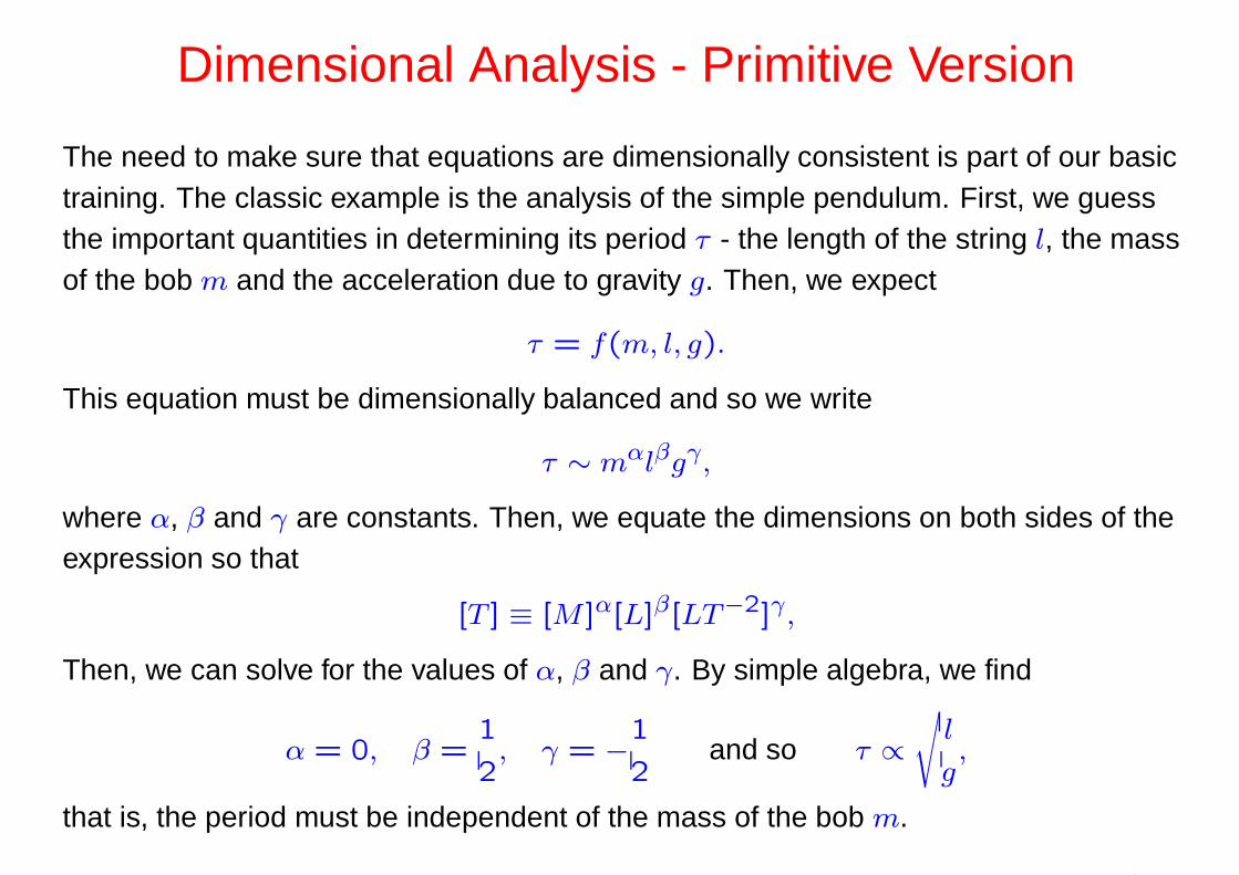
The need to make sure that equations are dimensionally consistent is part of our basictraining. The classic example is the analysis of the simple pendulum. First, we guessthe important quantities in determining its period τ - the length of the string l, the massof the bob m and the acceleration due to gravity g. Then, we expect
τ = f(m, l, g).
This equation must be dimensionally balanced and so we write
τ ∼ mαlβgγ,
where α, β and γ are constants. Then, we equate the dimensions on both sides of theexpression so that
[T ] ≡ [M ]α[L]β[LT−2]γ,
Then, we can solve for the values of α, β and γ. By simple algebra, we find
α = 0, β =1
2, γ = −
1
2and so τ ∝
√
l
g,
that is, the period must be independent of the mass of the bob m.
3

Dimensional Analysis - Superior Version
Dimensional analysis is, however, very much deeper than that and can help us to solvecomplicated problems without having to solve the complicated equations. The basicrule is:
• Guess what the important quantities are in the problem and form from thesedimensionless combinations – we will call these dimensionless groups.
We need the Buckingham Π Theorem
• A system described by n variables, built from r independent dimensions isdescribed by (n − r) independent dimensionless groups.
4

The Simple Pendulum
We first need to guess what the independent variables are likely to be. Here is a listwith their dimensions.
Variables which may determine the period of a pendulum
Variable Units Descriptionθ0 – angle of releasem [M] mass of bobτ [T] period of pendulumg [L][T]−2 acceleration due to gravityl [L] length of pendulum
From the Buckingham Π Theorem, there are five variables and three independentdimensions ([L], [T], [M]) and so we can form two independent dimensionless groups.
5
The Simple Pendulum
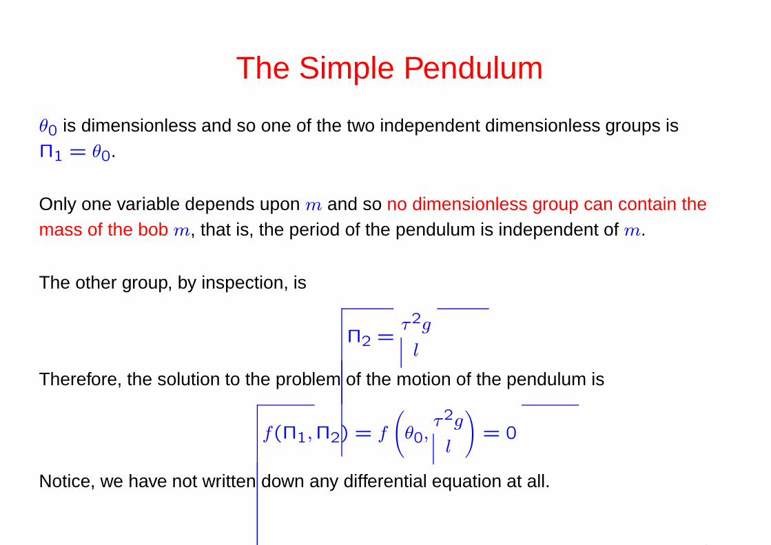
θ0 is dimensionless and so one of the two independent dimensionless groups isΠ1 = θ0.
Only one variable depends upon m and so no dimensionless group can contain themass of the bob m, that is, the period of the pendulum is independent of m.
The other group, by inspection, is
Π2 =τ2g
l
Therefore, the solution to the problem of the motion of the pendulum is
f(Π1,Π2) = f
(
θ0,τ2g
l
)
= 0
Notice, we have not written down any differential equation at all.
6
The General Pendulum
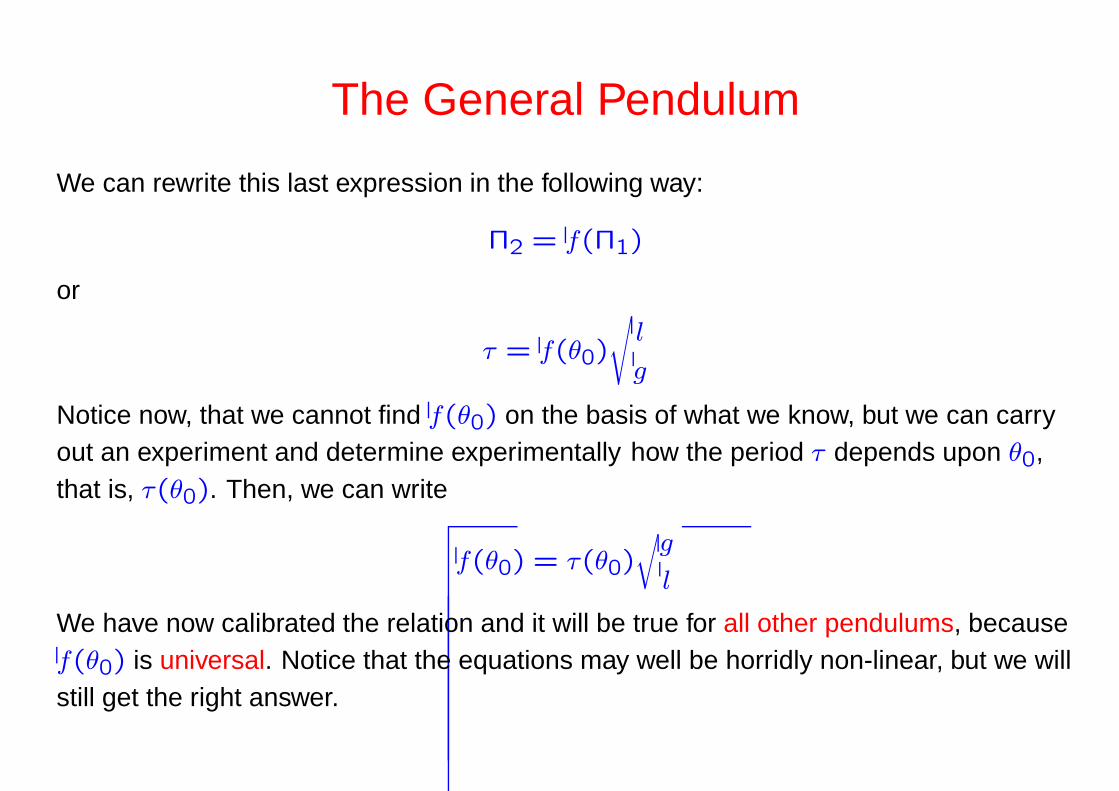
We can rewrite this last expression in the following way:
Π2 = f(Π1)
or
τ = f(θ0)
√
l
g
Notice now, that we cannot find f(θ0) on the basis of what we know, but we can carryout an experiment and determine experimentally how the period τ depends upon θ0,that is, τ(θ0). Then, we can write
f(θ0) = τ(θ0)
√
g
l
We have now calibrated the relation and it will be true for all other pendulums, becausef(θ0) is universal. Notice that the equations may well be horridly non-linear, but we willstill get the right answer.
7

The ‘Simple’ Pendulum
We can work out the exact answer for an arbitrary value of θ0. By conservation ofenergy,
mgl(1 − cos θ) + 12Iθ̇2 = const = mgl(1 − cos θ0)
where I = ml2 ; θ0 is the maximum amplitude of the pendulum. For small θ0, thisbecomes
θ̈ +g
lθ = 0
and so
ω =
√
g
lτ =
2π
ω= 2π
√
l
g
In general, we find,
θ̇ =
√
2g
l(cos θ − cos θ0)
1/2
with solution
τ =
√
2l
g
∫ 0
θ0
dθ
(cos θ − cos θ0)1/2
=
√
l
gf(θ0)
8

The Non-linear Pendulum
The diagram shows the exact solutionfor the non-linear pendulum
τ =
√
l
gf(θ0)
in terms of the dimensionless functionf(θ0).
9

Explosions
In 1950, G.I. Taylor carried out a classic analysis of the dynamics of the shock wavesassociated with nuclear explosions. A huge amount of energy E is released resulting inan enormous pressure within the spherical shock front. The external pressure istherefore irrelevant, but the dynamics of the shock front should depend upon theexternal density ρ0. The only other parameters in the problem are the radius of theshock front rf and the time t from the explosion. Hence, the table
Variable Units DescriptionE [M][L]2[T]−2 Energy releaseρ0 [M][L]−3 external densityrf [L] shock front radiust [T] time from the explosion
From the Buckingham Π Theorem, there are four variables and three independentdimensions and so we can form only one independent dimensionless group.
10

G.I. Taylor’s Analysis of Explosions
We find the relevant dimensionless quantity in the usual way. From the quotient of E
and ρ0, we find[
E
ρ0
]
=[M][L]2[T]−2
[M][L]−3=
[L5]
[T2]=
[
r5ft2
]
Thus,
Π1 =Et2
ρ0r5fand f
(
Et2
ρ0r5f
)
= 0
Thus, the simplest form of the relation to test is
rf = A
(
E
ρ0
)1/5
t2/5
where A is a constant.
11

G.I. Taylors Analysis of Atomic Explosions
This agrees beautifully with G.I.Taylor’s analysis of Mack’s movie of the explosion. Tothe annoyance of the US government, Taylor worked out E from the unclassified movieand found it to be about 1014 J.
12

Fluid Dynamics - Drag in Fluids
Let us apply the same techniques to the flow of an incompressible fluid about a sphere.This is encountered in deriving Stokes’ formula for the terminal velocity of sphere fallingthrough a viscous liquid. In the cases we study, the Navier-Stokes equations are:
∂v
∂t+ (v · ∇)v = −
1
ρ∇p + ν∇2
v
∇ · v = 0
In this form ν is the kinematic viscosity. This is the rather nasty set of non-linearequations which need to be solved. Let us develop the solution for the drag force usingdimensional arguments. First of all, we will consider the case in which viscosityprovides the retarding force and then the case in which the inertia of the fluid is thedominant force.
13

Viscous Drag
First, we list the variables which are important in determining the drag force on asphere moving steadily through a viscous fluid at terminal velocity v. The mass of thesphere will not appear in the drag force, since the force is acting on the surface of thesphere. It will appear when we equate the drag force to the gravitational force.
Variable Units DescriptionFd [M][L][T]−2 Drag forceρf [M][L]−3 density of fluidR [L] radius of sphereν [L2][T]−1 kinematic viscosityv [L][T]−1 terminal velocity
From the Buckingham Π Theorem, there are 5 variables and three independentdimensions and so we can form two independent dimensionless groups.
14

Stokes’ Formula
The last three entries in the table clearly form one dimensionless group. By inspection,
Π1 =vR
ν= Re
This is the Reynold’s number. It is a dimensionless measure of the speed of the sphere.
The second dimensionless group must involve the first two entries in the table.Obviously, the dimensionless quantity
Π2 =Fd
ρfR2v2
can be constructed. The most general relation is f(Π1,Π2) = 0 and, since we want tofind an expression for Fd, let us write
Π2 = f(Π1)
that is,
Fd = ρfR2v2f
(
vR
ν
)
15

Stokes’ Formula
Now, the drag force should be proportional to the viscosity ν and so the function f̄(x)
must be proportional to 1/x. Therefore, our expression for the drag force is
Fd = AρfR2v2
(
vR
ν
)−1
= AνρfRv
where A is a constant to be found. We cannot do any better by these techniques.Going through the full analysis, A = 6π and so
Fd = 6πνρfRv
Now equating this drag force to the gravitational force on the sphere,Fg = (4π/3)ρspR3g, we get the final answer
(4π/3)ρspR3g = 6πνρfRv
that is,
v =2
9
(
gR2
ν
)(
ρsp
ρf
)
This is Stokes’ Formula.
16
The Effect of Buoyancy
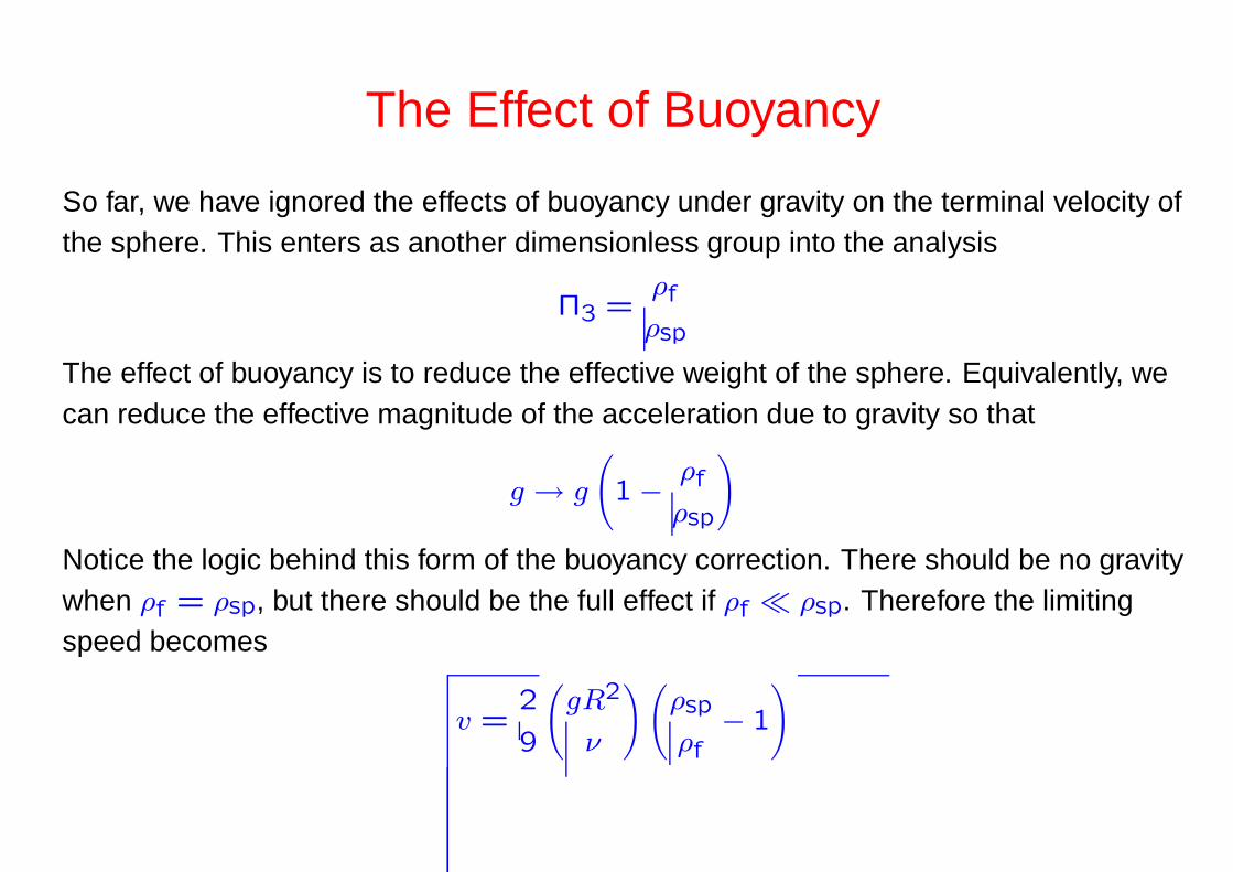
So far, we have ignored the effects of buoyancy under gravity on the terminal velocity ofthe sphere. This enters as another dimensionless group into the analysis
Π3 =ρf
ρsp
The effect of buoyancy is to reduce the effective weight of the sphere. Equivalently, wecan reduce the effective magnitude of the acceleration due to gravity so that
g → g
(
1 −ρf
ρsp
)
Notice the logic behind this form of the buoyancy correction. There should be no gravitywhen ρf = ρsp, but there should be the full effect if ρf ≪ ρsp. Therefore the limitingspeed becomes
v =2
9
(
gR2
ν
)(
ρsp
ρf− 1
)
17

Terminal Speed in the High Reynolds’ Number Limit
In the high Reynolds’ number limit, Re = vR/ν ≫ 1, the flow past the spherebecomes turbulent. Then, the viscosity is unimportant in determining the flow of thefluid past the sphere. The viscous forces transfer momentum by diffusion, as can beseen from the form of the time-dependent Navier-Stokes equation
∂v
∂t+ (v · ∇)v = ν∇2
v
The characteristic time for the diffusion of the viscous stresses is found to order ofmagnitude by approximating
v
tν≈
νv
R2tν ≈
R2
ν
The time for the fluid to flow past the sphere is tv = R/v. The condition Re ≫ 1
corresponds to tv ≪ tν .
18

Terminal speed at Re ≫ 1
Thus, we can drop the viscosity from our table of relevant parameters.
Variable Units DescriptionFd [M][L][T]−2 Drag forceρf [M][L]−3 density of fluidR [L] radius of spherev [L][T]−1 terminal velocity
There are 4 variables and three independent dimensions and so we can form only oneindependent dimensionless group which we have found already.
Π2 =Fd
ρfR2v2
Therefore, we write
f
(
Fd
ρfR2v2
)
= 0 and try Fd = Aρfv2R2
where A is a constant of order unity.
19

Terminal speed at Re ≫ 1
There is a simple interpretation is the formula Fd = ρfv2R2. This is simply the rate at
which the momentum of the fluid is being pushed away by the sphere per second.Equating this to the gravitational force, we find
Fd = ρfv2R2 =
4πR3
3(ρsp − ρf)g
and so
v ≈
√
√
√
√gR(ρsp − ρf)
ρf
Conventionally, the drag force is written
Fd = 12cdρfv
2Aproj
where Aproj is the projected surface area and cd is the drag coefficient. Here are somevalues:
Object cd Object cdSphere 0.5 Flat plate 2.0Cylinder 1.0 Car 0.4
20

Flow past a Sphere in the Viscous andInertial Limits
Viscous flow past sphere at Re ≪ 1.
Turbulent flow past a sphere atRe = 117.
Drag as a function of Reynolds numbersRe
The dashed line shows Stokes’ lawwhich can be rewritten
cD =12π
Re.
21

Kolmogorov Spectrum of Turbulence
Turbulence is one of the great unsolved problems of fluid dynamics. Energy is fed in onthe large scales and is then degraded by turbulent eddies into smaller and smallerscales until it is dissipated by molecular viscosity. The spectrum is thereforecharacterised by the transfer of energy from large to small scales.
Let E(k) dk be the energy contained in eddies per unit mass in the wavenumberinterval k to k + dk. Suppose the kinetic energy input per unit mass is ε0. We can formthe usual table.
Variable Units DescriptionE(k) [L]3[T]−2 Energy per unit wavenumber per unit massε0 [L]2[T]−3 rate of energy input per unit massk [L]−1 wavenumber
There are 3 variables and two independent dimensions and so we can form only oneindependent dimensionless group.
22

Kolmogorov Spectrum of Turbulence
We find
Π1 =E3(k)k5
ε20
and so we expect
E(k) ∝ ε2/3k−5/3
This turns out to be a remarkably goodfit to the spectrum of turbulence onscales on which k0 and viscosity can beneglected.
23
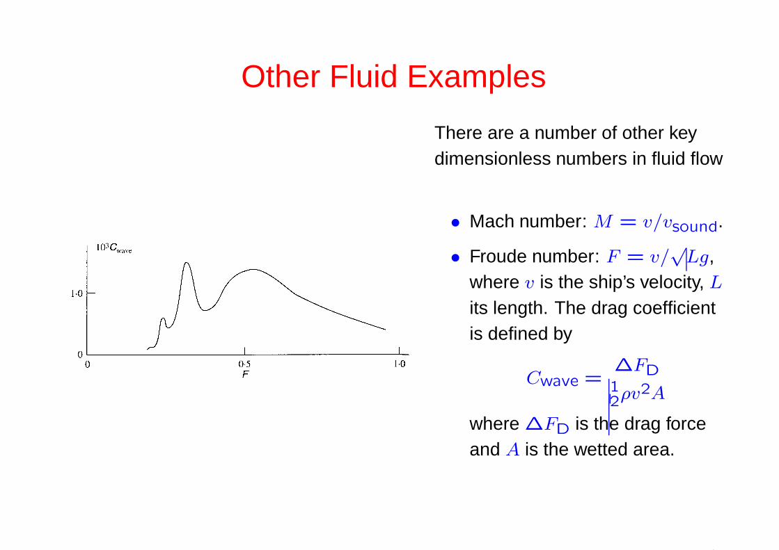
Other Fluid Examples
There are a number of other keydimensionless numbers in fluid flow
• Mach number: M = v/vsound.
• Froude number: F = v/√
Lg,where v is the ship’s velocity, L
its length. The drag coefficientis defined by
Cwave =∆FD12ρv2A
where ∆FD is the drag forceand A is the wetted area.
24

The Law of Corresponding States
We can use dimensionaltechniques to understand thelaw of corresponding states.The gas is imperfect and weneed to take account of the finitesize of the molecules and thedepth of the attractive potentialbetween the molecules. In thediagram, we characterise theseby the intermolecular separationσ and the depth of the potentialwell ∆ε.
25

The Law of Corresponding States
Now, list all the variables in the problem.
Variable Units Descriptionp [M][L]−1[T]−2 PressureV [L]3 VolumekT [M][L]2[T]−2 ‘Temperature’N – Number of moleculesm [M] Mass of moleculeσ [L] Intermolecular spacing∆ε [M][L]2[T]−2 Depth of attractive
potential
26

The Reduced Equation of State
There are therefore four independent dimensionless numbers. There are now lots ofways of combining these and so let me choose a simple set of four to begin with. I havebeen guided by the need to relate macroscopic quantities to microscopic quantities inthe choice of the Πs.
Π1 = N Π2 =kT
∆εΠ3 =
V
σ3Π4 =
pσ3
∆ε
Notice that there is no way that m can be included in the four dimensionless quantities.The imperfect gas law is independent of the mass of the molecules.
We now need to include some physics into the analysis. The equation of state involvesonly three quantities, but we have four independent variables. Now, p and T areintensive variables which are independent of the ‘extent’ of the system. V is anextensive variable. Suppose we cut the system in half. Then, the volume and thenumbers of particles in each half are both halved. Therefore, the equation of state canonly involve the ratio Π5 = V/Nσ3, which is the ratio of the volume to the volumeoccupied by the molecules themselves.
27

The Reduced Equation of State
Therefore, we can write
Π4 = f(Π1,Π2,Π3) or Π4 = f(Π2,Π5)
pσ3
∆ε= f
(
V
Nσ3,kT
∆ε
)
p
p∗= f
(
V
V ∗,T
T ∗
)
where
p∗ =∆ε
σ3V ∗ = Nσ3 T ∗ =
∆ε
k.
Furthermore, we see that p∗V ∗/NkT ∗ = 1.
28
The Reduced Equation of State
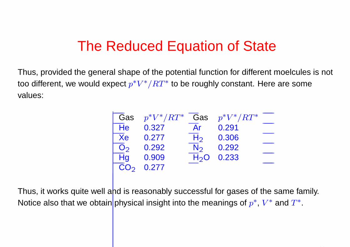
Thus, provided the general shape of the potential function for different moelcules is nottoo different, we would expect p∗V ∗/RT ∗ to be roughly constant. Here are somevalues:
Gas p∗V ∗/RT ∗ Gas p∗V ∗/RT ∗
He 0.327 Ar 0.291Xe 0.277 H2 0.306O2 0.292 N2 0.292Hg 0.909 H2O 0.233CO2 0.277
Thus, it works quite well and is reasonably successful for gases of the same family.Notice also that we obtain physical insight into the meanings of p∗, V ∗ and T ∗.
29

The Law of Corresponding States
The Law of Corresponding States is the statement that the reduced equations of stateare of the same form for all gases. For example, the van der Waals and Dietericiequations of state can be written
van der Waals
(
π +3
φ2
)
(3φ − 1) = 8θ
and
Dieterici π(2φ − 1) = θ exp
[
2
(
1 −1
θφ
)]
where π = p/p∗, φ = V/V ∗ and θ = T/T ∗.
30

Other Examples
There are many more examples which could be given from physics
• Lindemann’s law of melting.
• Critical phenomena in phase transitions, for example, the ferromagnetic transition.
In addition, there are similarity solutions of the equations, which keep the same overallform as the dimensionless parameters are changed. For many beautiful examples ofthese techniques, see Scaling, self-similarity, and intermediate asymptotics by G.I.Barenblatt. For example, show that the speed of a rowing boat is proportional to theN1/9 where N is the number of rowers.
31


