Dimensionality Estimation and Manifold

Learning using Tensor Voting

Philippos Mordohai and Gerard Medioni

Institute for Robotics and Intelligent Systems, University of Southern California,Los Angeles, CA 90083-0273, USA Email: {mordohai, medioni}@iris.usc.edu

Abstract

We address instance-based learning from a perceptual organization standpoint us-ing tensor voting. The goal of instance-based learning is to learn the underlyingrelationships between observations, which are points in an N -D continuous space,under the assumption that they lie in a limited part of the N -D space, typicallya manifold, the dimensionality of which is an indication of the degrees of freedomof the underlying system. We pose the problem of instance-based learning in anequivalent form: manifold learning from observations. Unlike traditional manifoldlearning approaches, we do not perform dimensionality reduction, which would limitthe class of datasets we are able to process, but instead perform all operations inthe original input space. To this end we apply tensor voting, a perceptual organi-zation framework that has mostly been applied to computer vision problems, aftermodifying it to make its implementation in high-dimensional spaces practical.

We are able to estimate local dimensionality and structure for datasets that can-not be handled by current state-of-the-art approaches. We first show that we can ob-tain reliable dimensionality estimates at each point, instead of a global average esti-mate for the entire dataset, which is a major advantage over competing methods. Wethen present a quantitative evaluation of our results in the estimation of local man-ifold structure using synthetic datasets with known ground truth. Our software isavailable to the scientific community at http://iris.usc.edu/home/iris/medioni/User.html.

1 Introduction

Machine learning is a research area in artificial intelligence that aims at theimprovement of the behavior of agents through diligent study of observations[1]. It deals with the development of algorithms that analyze the observed datato identify patterns and relationships, in order to predict unseen data. Here, weaddress a subfield of machine learning that operates in continuous domains andlearns from observations that are represented as points in a Euclidean space.

This type of learning is termed instance-based or memory-based learning [2].Learning in discrete domains, which attempts to infer the states, transitionsand rules that govern a system, or the decisions and strategies that maximizea utility function, is out of the scope of our research.

The problem of learning a target function based on instances is equivalent tolearning a manifold formed by a set of points, and thus being able to predictthe positions of other points on the manifold. The first task, given a set ofobservations, is to determine the intrinsic dimensionality of the data. This canprovide insight for the complexity of the system that generates the data, thetype of model needed to describe them, as well as the actual degrees of free-dom of the system, which are not necessarily equal with the dimensionality ofthe input space. We also estimate the orientation of a potential manifold thatpasses through each point. Both of these tasks are accomplished simultane-ously by encoding the observations as symmetric, second order, nonnegativedefinite tensors and analyzing the results of tensor voting [3]. Since the processthat estimates dimensionality and orientation is performed on the inputs, ourapproach falls under the “eager learning” category, according to Mitchell [2].Unlike other eager approaches, however, ours is not global. This offers consid-erable advantages when the data become more complex, or when the numberof instances is large. The main characteristic of eager, instance-based learningmethods is that the query points are not taken into account when decisionsare made. In other words, the orientation of each training sample is estimatedduring the training stage, and the fact that a previously unseen point alsobelongs to the manifold does not alter these estimates. Assuming that thedistribution of the data is stationary, this does not cause any difficulties. Ifstationarity does not hold, however, learning has to be accompanied by updateand a forgetting mechanisms. This is out of the scope of this paper, but it isa rather straightforward extension of our work.

All processing is performed using tensor voting, which is a computationalframework for perceptual organization based on the Gestalt principles of prox-imity and good continuation [3]. It has mainly been applied to organize genericpoints (tokens) into coherent groups and for computer vision problems thatwere formulated as perceptual organization tasks. For instance, the problemof stereo vision can be formulated as the organization of potential pixel corre-spondences into salient surfaces, under the assumption that correct correspon-dences form coherent surfaces and wrong ones do not [4]. Salient structuresare inferred based on the support the tokens receive from their neighbors inthe form of votes, which are also second order tensors that are cast fromeach token to all other tokens within its neighborhood. Each vote conveysthe orientation the receiver would have if the voter and receiver were in thesame structure. The concepts of proximity and good continuation also applyin high-dimensional spaces and the absence of global computations makes ourmethod suitable for processing large datasets. In Section 3, we propose a new

2

implementation of tensor voting that is not limited to low-dimensional spacesas the original one of [3].

Instance-based learning has recently received renewed interest from the ma-chine learning community, due to its many applications in the fields of patternrecognition, data mining, kinematics, function approximation and visualiza-tion, among others. This interest was sparked by a wave of new algorithms thatadvanced the state of the art and are capable of learning nonlinear manifoldsin spaces of very high dimensionality. These include kernel PCA [5], locallylinear embedding (LLE) [6], Isomap [7] and charting [8], which are reviewedin Section 2. They aim at reducing the dimensionality of the input space ina way that preserves certain geometric or statistical properties of the data.Isomap, for instance, attempts to preserve the geodesic distances between allpoints as the manifold is “unfolded” and mapped to a space of lower dimen-sion. A common assumption is that the desired manifold consists of locallylinear patches. We relax this assumption by only requiring that manifolds besmooth almost everywhere. Smoothness in this context is the property of themanifold’s orientation to vary gradually as one moves from point to point.This property is encoded in the votes that each point casts to its neighbors.

We take a different path to learning low dimensional manifolds from instancesin a high dimensional space. Whereas traditional methods address the problemas one of dimensionality reduction, we propose an approach for the unsuper-vised learning of manifold structure in a way that is useful for tasks such asgeodesic distance estimation and nonlinear interpolation, that does not em-bed the data in a lower dimensional space. We compute local dimensionalityestimates, but instead of performing dimensionality reduction, we performall operations in the original input space, taking into account the estimateddimensionality of the data. This allows us to process datasets that are notmanifolds globally, or ones with varying intrinsic dimensionality. The latterpose no additional difficulties, since we do not use a global estimate for the di-mensionality of the data. Results have been presented in our previous work [9].Moreover, outliers, boundaries, intersections or disconnected components arehandled naturally as in 2-D and 3-D [3, 10]. Non-manifolds, such as hyper-spheres, can also be processed without any modifications of the algorithmsince we do not attempt to estimate a global “unfolding”. Quantitative resultsfor the robustness against outliers that outnumber the inliers are presentedin Section 6. Once processing with tensor voting has been completed, dimen-sionality reduction can be performed using any of the approaches described inthe next section. Tensor voting can remove outliers and provide reliable localestimates of dimensionality that are useful for segmenting the data in smoothcomponents for subsequent processing. Dimensionality reduction reduces thestorage requirements for the processed dataset.

This document is organized as follows: an overview of related work is given in

3

the next section; the new N -D implementation of tensor voting is presented inSection 3; the new implementation is compared with the one of [3] in Section4; results in dimensionality estimation are presented in Section 5, while resultsin local structure estimation are presented in Section 6; Section 7 concludesthe paper. Appendix A is a simple user’s manual for the executable, whileAppendix B is the license agreement for the Approximate Nearest Neighbor(ANN) k-d tree library (release 0.1) [11] that is used as the datastructure thatstores and searches through the data.

2 Related Work

In this section, we present related work in the domains of dimensionality es-timation and manifold learning.

Dimensionality Estimation Bruske and Sommer [12] present an approachfor dimensionality estimation where an optimally topology preserving map(OTPM) is constructed for a subset of the data, which is produced after vectorquantization. Principal Component Analysis (PCA) is then performed for eachnode of the OTPM under the assumption that the underlying structure of thedata is locally linear. The average of the number of significant singular valuesat the nodes is the estimate of the intrinsic dimensionality.

Kegl [13] estimates the capacity dimension of the manifold, which does notdepend on the distribution of the data, and is equal to the topological dimen-sion, using an efficient approximation based on packing numbers. The algo-rithm takes into account dimensionality variations with scale, and is basedon a geometric property of the data, rather than successive projections to in-creasingly higher-dimensional subspaces until a certain percentage of the datais explained.

Costa and Hero [14] estimate the intrinsic dimension of the manifold and theentropy of the samples using geodesic-minimal-spanning trees. The method,similarly to Isomap [7], considers global properties of the adjacency graph andthus produces a single global estimate.

Levina and Bickel [15] compute maximum likelihood estimates of dimension-ality by examining the number of neighbors included in spheres the radiusof which is selected in such a way that the density of the data contained inthem can be assumed constant, and enough neighbors are included. Theserequirements cause an underestimation of the dimensionality when it it veryhigh.

4

Manifold Learning Here, we briefly present recent approaches for learninglow dimensional embeddings from points in high dimensional spaces. Mostof them are extensions of linear techniques, such as Principal ComponentAnalysis (PCA) [16] and Multi-Dimensional Scaling (MDS) [17], based on theassumption that nonlinear manifolds can be approximated by locally linearpatches.

In contrast to other methods, Scholkopf et al. [5] propose kernel PCA thatattempts to find linear patches using PCA in a space of typically higher di-mensionality than the input space. Correct kernel selection can reveal the lowdimensional structure of the input data after mapping the instances to a spaceof higher dimensionality. For instance a second order polynomial kernel canreveal quadratic surfaces since they appear as planes in the high-dimensionalspace.

Locally Linear Embedding (LLE) was presented by Roweis and Saul [6, 18].The underlying assumption is that if data lie on a locally linear, low-dimensionalmanifold, then each point can be reconstructed from its neighbors with appro-priate weights. These weights should be the same in a low-dimensional space,the dimensionality of which is greater or equal to the intrinsic dimensionalityof the manifold, as long as the manifold is locally linear. The LLE algorithmcomputes the basis of such a low-dimensional space. The dimensionality of theembedding, however, has to be given as a parameter, since it cannot alwaysbe estimated from the data [18]. Moreover, the output is an embedding ofthe given data, but not a mapping from the ambient to the embedding space.Global coordination of the local embeddings, and thus a mapping, can becomputed according to [19]. LLE is not isometric and often fails by mappingdistant points close to each other.

Tenenbaum et al. [7] propose Isomap, which is an extension of MDS that usesgeodesic instead of Euclidean distances. This allows Isomap to handle nonlin-ear manifolds, whereas MDS is limited to linear data. The geodesic distancesbetween points are approximated by graph distances. Then, MDS is applied onthe geodesic distances to compute an embedding that preserves the propertyof points to be close or far away from each other. Due to its global formu-lation, Isomap’s computational cost is considerably higher than that of LLE.The benefit is that not only it preserves distances between nearest neighbors,but between all points. In addition, it can handle points not in the originaldataset, and perform interpolation. C-Isomap, a variation of Isomap that canbe applied to data with intrinsic curvature, but known distribution, and L-Isomap, a faster alternative that only uses a few landmark point for distancecomputations, have also been proposed in [20]. Isomap and its variants arelimited to convex datasets.

Laplacian Eigenmaps were proposed by Belkin and Niyogi [21] who compute

5

the normalized graph Laplacian of the adjacency graph of the input data.It is an approximation of the Laplace-Beltrami operator on the manifold,and exploit its locality preserving properties that were first observed in thefield of clustering. The Laplacian eigenmaps algorithm can be viewed as ageneralization of LLE, since the two become identical when the weights ofthe graph are chosen according to the criteria of the latter. Much like LLE,the dimensionality of the manifold also has to be provided, the computedembeddings are not isometric and a mapping between the two spaces is notproduced. The latter is addressed in [22] where a variation of the algorithm isproposed.

Donoho and Grimes [23] propose Hessian LLE (HLLE), an approach similarto the above, which computes the Hessian instead of the Laplacian of thegraph. The authors claim that the Hessian is better suited than the Laplacianin detecting linear patches on the manifold. The major contribution of thisapproach is that it proposes a global, isometric method, which, unlike Isomap,can be applied to non-convex datasets. The need to estimate second derivativesfrom possibly noisy, discrete data makes the algorithm more sensitive to noisethan the others reviewed here.

Semidefinite Embedding (SDE) was proposed by Weinberger and Saul [24]who address the problem of manifold learning by enforcing local isometry.The lengths of the sides of triangles formed by neighboring points are pre-served during the embedding. These constraints can be expressed in terms ofpairwise distances and the optimal embedding can be found by semidefiniteprogramming. The method is the most computationally demanding reviewedhere, but can reliably estimate the underlying dimensionality of the inputs bylocating the largest gap between the eigenvalues of the Gram matrix of theoutputs. Similarly to our approach, this estimate does not require a thresh-old, as do approaches that estimate the residual error as a function of thedimensionality of the fitted model.

Other research related to ours includes the charting algorithm of Brand [8].It computes a pseudo-invertible mapping of the data, as well as the intrinsicdimensionality of the manifold, which is estimated by examining the rate ofgrowth of the number of points contained in hyper-spheres as a function ofthe radius. Linear patches, areas of curvature and noise can be discriminatedusing the proposed measure. Affine transformations that align the coordinatesystems of the linear patches are computed at the second stage. This defines aglobal coordinate system for the embedding and thus a mapping between theinput space and the embedding space.

Wang et al. [25] propose an adaptive version of the local tangent space align-ment (LTSA) of Zhang and Zha [26], a local dimensionality reduction methodthat is a variation of LLE. Wang et al. address a limitation of most of the

6

approaches presented in this section, which is the use of a fixed number ofneighbors for all points in the data. This causes serious problems if that num-ber is not selected properly, near boundaries, or if the density of the datais not approximately constant. The authors propose a method to adapt theneighborhood size according to local criteria and demonstrate its effective-ness on datasets of varying distribution. The adaptive number of neighborsat each point is an important contribution in the field of manifold learning,since the contributions of each neighbor are typically not weighted, makingthe algorithms very sensitive to the selection of k.

The difference between our approach and those of [8, 12–15, 24] is that oursproduces reliable dimensionality estimates at the point level, which do nothave to be averaged over the entire dataset. While this is not important fordatasets with constant dimensionality, the ability to estimate local dimen-sionality reliably becomes a key factor when dealing with data generated bydifferent unknown processes. Given reliable local estimates, the dataset canbe segmented in components with constant dimensionality. An advantage ofapproaches that perform dimensionality reduction over ours is a potentiallysubstantial reduction in memory requirements.

3 Tensor Voting in High Dimensional Spaces

The tensor voting framework, in its preliminary version [27], is an attemptat the implementation of two Gestalt principles, namely proximity and goodcontinuation, for grouping generic tokens in 2-D. The 2-D domain has alwaysbeen the main focus of research in perceptual organization, beginning with theresearch of Kohler [28], Wertheimer [29] and Koffka [30]. The generalizationto 3-D is straightforward, since salient groupings can be detected by the hu-man visual system based on the same principles. Guy and Medioni extendedthe framework to three dimensions in [31]. Regardless of the computationalfeasibility of an implementation, the same grouping principles apply to spaceswith even higher dimensions. For instance, Tang et al. [32] observed that pixelcorrespondences can be viewed as points in the 8-D space of free parametersof the fundamental matrix. Correct correspondences align to form a hyper-plane in that space, while wrong correspondences are randomly distributed.By applying tensor voting in 8-D, the authors were able to infer the dominanthyperplane and the desired parameters of the fundamental matrix. Storageand computation requirements, however, soon become prohibitively high asthe dimensionality of the space increases.

Even though the applicability of tensor voting, as implemented in [3], as amanifold learning technique in high-dimensional spaces seems to have merit, ageneral implementation is not practical, mostly due to computational complex-

7

ity and storage requirements inN dimensions. The bottleneck is the generationand storage of voting fields, the number of which is equal to the dimension-ality of the space. The voting fields are used as look-up tables to retrievepre-computed votes via interpolation between the pre-computed samples. Forinstance, a voting field in 10-D with k samples per axis, requires storage fork10 10×10 tensors, which need to be computed via numerical integration over10 variables. Thus, the pre-computed voting fields become impractical as di-mensionality grows. Here, we propose a simplified vote generation scheme thatallows the generation of votes from arbitrary tensors in arbitrary dimensionswith a computational cost that is linear with respect to the dimensionalityof the space. Storage requirements are limited to storing the tensors at eachtoken since voting fields are not used any more.

In this section, we describe the tensor voting framework beginning with datarepresentation and proceeding to the voting mechanism and vote analysis.The representation and vote analysis schemes are the same as in the origi-nal implementation [3]. The contribution of this section is the introductionof a new formulation of the voting process that is practical for spaces of di-mensionality up to a few hundreds. Efficiency is considerably higher than ourinitial attempt in [9], where we focused on dimensionality estimation, but theproposed approximation to vote generation is slower than the one proposedhere.

3.1 Data Representation

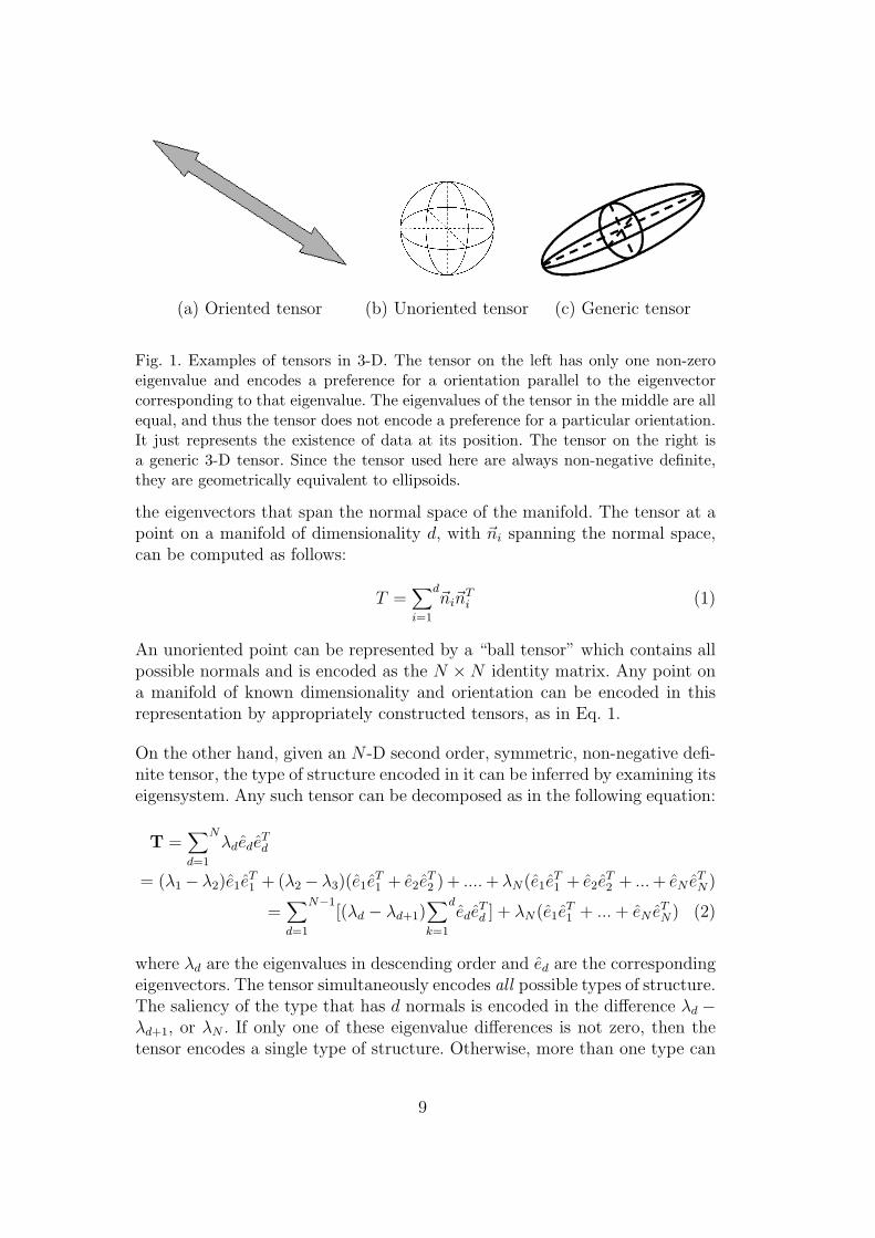
The representation of a point is a second order, symmetric, non-negative defi-nite tensor, which is equivalent to an N×N matrix and an ellipsoid in an N -Dspace. All tensors in this paper are second order, symmetric and non-negativedefinite, so any reference to a tensor automatically implies these properties.Three examples of tensors, in 3-D, can be seen in Fig. 1. A tensor can representthe structure of a manifold going through the point by encoding the normalsto the manifold as eigenvectors of the tensor that correspond to nonzero eigen-values, and the tangents as eigenvectors that correspond to zero eigenvalues.A point in an N -D hyperplane has one normal and N−1 tangents, and thus isrepresented by a tensor with one nonzero eigenvalue associated with an eigen-vector parallel to the hyperplane’s normal. The remaining N − 1 eigenvaluesare zero. A point in a 2-D manifold in N -D has two tangents and N − 2 nor-mals, and thus is represented by a tensor with two zero eigenvalues associatedwith the eigenvectors that span the tangent space of the manifold. The tensoralso has N − 2 nonzero eigenvalues (typically set to 1) whose correspondingeigenvectors span the manifold’s normal space.

The tensors can be formed by the summation of the direct products (~n~nT ) of

8

(a) Oriented tensor (b) Unoriented tensor (c) Generic tensor

Fig. 1. Examples of tensors in 3-D. The tensor on the left has only one non-zeroeigenvalue and encodes a preference for a orientation parallel to the eigenvectorcorresponding to that eigenvalue. The eigenvalues of the tensor in the middle are allequal, and thus the tensor does not encode a preference for a particular orientation.It just represents the existence of data at its position. The tensor on the right isa generic 3-D tensor. Since the tensor used here are always non-negative definite,they are geometrically equivalent to ellipsoids.

the eigenvectors that span the normal space of the manifold. The tensor at apoint on a manifold of dimensionality d, with ~ni spanning the normal space,can be computed as follows:

T =∑i=1

d~ni~n

Ti (1)

An unoriented point can be represented by a “ball tensor” which contains allpossible normals and is encoded as the N ×N identity matrix. Any point ona manifold of known dimensionality and orientation can be encoded in thisrepresentation by appropriately constructed tensors, as in Eq. 1.

On the other hand, given an N -D second order, symmetric, non-negative defi-nite tensor, the type of structure encoded in it can be inferred by examining itseigensystem. Any such tensor can be decomposed as in the following equation:

T =∑d=1

Nλdede

Td

= (λ1 − λ2)e1eT1 + (λ2 − λ3)(e1e

T1 + e2e

T2 ) + ....+ λN(e1e

T1 + e2e

T2 + ...+ eN e

TN)

=∑d=1

N−1[(λd − λd+1)

∑k=1

dede

Td ] + λN(e1e

T1 + ...+ eN e

TN) (2)

where λd are the eigenvalues in descending order and ed are the correspondingeigenvectors. The tensor simultaneously encodes all possible types of structure.The saliency of the type that has d normals is encoded in the difference λd −λd+1, or λN . If only one of these eigenvalue differences is not zero, then thetensor encodes a single type of structure. Otherwise, more than one type can

9

be present at the location of the tensor, each having a saliency value givenby the appropriate difference between consecutive eigenvalues of λN . If a harddecision on dimensionality is required, the location can be assigned to the typewith the maximum saliency.

3.2 The Voting Process

After the inputs have been encoded with tensors, they are stored in an Approx-imate Nearest Neighbor (ANN) k-d tree data structure, which was proposedby Arya et al. [11]. The information they contain is propagated to their neigh-bors via a voting operation. For visualization purposes, the illustrations arefor the 2-D and 3-D cases. Given a tensor at A and a tensor at B, the vote thetoken at A (the voter) casts to B (the receiver) has the orientation the receiverwould have, if both the voter and receiver belonged to the same perceptualstructure. The magnitude of the vote is a function of the confidence we havethat the voter and receiver indeed belong to the same perceptual structure.

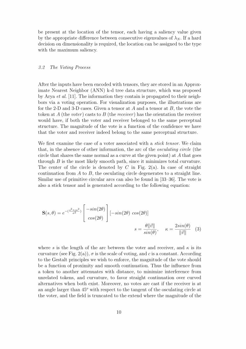
We first examine the case of a voter associated with a stick tensor. We claimthat, in the absence of other information, the arc of the osculating circle (thecircle that shares the same normal as a curve at the given point) at A that goesthrough B is the most likely smooth path, since it minimizes total curvature.The center of the circle is denoted by C in Fig. 2(a). In case of straightcontinuation from A to B, the osculating circle degenerates to a straight line.Similar use of primitive circular arcs can also be found in [33–36]. The vote isalso a stick tensor and is generated according to the following equation:

S(s, θ) = e−( s2+cκ2

σ2 )

−sin(2θ)

cos(2θ)

[−sin(2θ) cos(2θ)]

s =θ‖~v‖sin(θ)

, κ =2sin(θ)

‖~v‖(3)

where s is the length of the arc between the voter and receiver, and κ is itscurvature (see Fig. 2(a)), σ is the scale of voting, and c is a constant. Accordingto the Gestalt principles we wish to enforce, the magnitude of the vote shouldbe a function of proximity and smooth continuation. Thus the influence froma token to another attenuates with distance, to minimize interference fromunrelated tokens, and curvature, to favor straight continuation over curvedalternatives when both exist. Moreover, no votes are cast if the receiver is atan angle larger than 45o with respect to the tangent of the osculating circle atthe voter, and the field is truncated to the extend where the magnitude of the

10

vote is more than 3% of the magnitude of the voter. The scale of voting σ isthe only free parameter and essentially controls the range within which tokenscan influence other tokens. It can also be viewed as a measure of smoothness.A large scale favors long range interactions and enforces a higher degree ofsmoothness, aiding noise removal, while a small scale makes the voting processmore local, thus preserving details.

The computation of votes cast by stick voters is performed in a 2-D subspace,defined by the position of the voter and the receiver and the orientation of thevoter, regardless of the dimensionality of the input space. Thus, this operationis applicable to high-dimensional spaces as well.

On the other hand, votes from non-stick tensors are generated, in the originalformulation [3], by integrating the votes cast by a rotating stick tensor thatspans the normal space of the voting tensor. Since the resulting integral hasno closed form solution, the integration is approximated numerically by takingsample positions of the rotating stick tensor and adding the votes it generatesat each point within the voting neighborhood. As a result, votes that coverthe voting neighborhood are pre-computed and stored in voting fields. Thevoting fields are normalized so that their energy is equal to that of the stickvoting field and then used as look-up tables, from which the necessary votes areretrieved via linear interpolation. The advantage of this scheme is that all votesare generated based on the stick voting field. Its computational complexity,however, makes its application prohibitive in high-dimensional spaces.

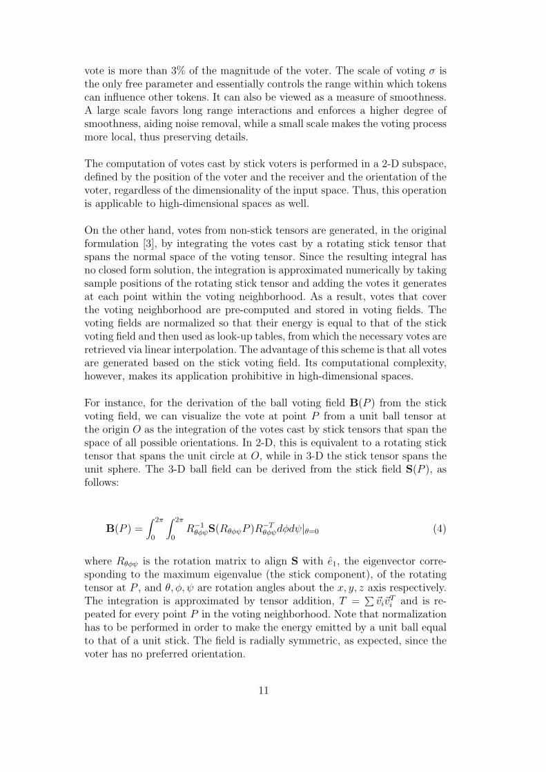
For instance, for the derivation of the ball voting field B(P ) from the stickvoting field, we can visualize the vote at point P from a unit ball tensor atthe origin O as the integration of the votes cast by stick tensors that span thespace of all possible orientations. In 2-D, this is equivalent to a rotating sticktensor that spans the unit circle at O, while in 3-D the stick tensor spans theunit sphere. The 3-D ball field can be derived from the stick field S(P ), asfollows:

B(P ) =∫ 2π

0

∫ 2π

0R−1θφψS(RθφψP )R−Tθφψdφdψ|θ=0 (4)

where Rθφψ is the rotation matrix to align S with e1, the eigenvector corre-sponding to the maximum eigenvalue (the stick component), of the rotatingtensor at P , and θ, φ, ψ are rotation angles about the x, y, z axis respectively.The integration is approximated by tensor addition, T =

∑~vi~v

Ti and is re-

peated for every point P in the voting neighborhood. Note that normalizationhas to be performed in order to make the energy emitted by a unit ball equalto that of a unit stick. The field is radially symmetric, as expected, since thevoter has no preferred orientation.

11

Here we describe a novel vote generation scheme that does not require integra-tion. As in the original formulation, the eigenstructure of the vote representsthe normal and tangent spaces that the receiver would have, if the voter andreceiver belong in the same smooth structure. What is missing is the uncer-tainty, which was included in each vote as a result of the accumulation of thevotes cast by the rotating stick tensors during the computation of the votingfields. The disagreement in the preferred orientation among these votes con-tributed to a non-zero ball component, which can be viewed as a measure ofuncertainty. On the other hand, the new votes are cast directly from the voterto the receiver and are not retrieved from pre-computed voting fields. Theyhave perfect certainty in the information they convey. The uncertainty nowcomes only from the accumulation of votes from different voters at each token.

As mentioned above, the generation of stick votes remains unchanged. Regard-ing the generation of ball votes, we propose the following direct computation.It is based on the observation that the vote generated by a ball voter propa-gates the voter’s preference for a straight line that connects it to the receiver(Fig. 2(b)). The straight line is the simplest and smoothest continuation froma point to another point in the absence of other information. Thus, the votegenerated by a ball voter is a tensor that spans the (N − 1)-D normal spaceof the line and has one zero eigenvalue associated with the eigenvector that isparallel to the line. Its magnitude is a function of only the distance between thetwo points, since curvature is zero. Taking these observations into account, theball vote can be constructed by subtracting the direct product of the tangentvector from a full rank tensor with equal eigenvalues (i.e. the identity matrix).The resulting tensor is attenuated by the same Gaussian weight according tothe distance between the voter and the receiver.

B(s, θ) = e−( s2

σ2 )(I − ~v~vT

‖~v~vT‖) (5)

where ~v is a unit vector parallel to the line connecting the voter and the

(a) Stick voting (b) Ball voting

Fig. 2. Vote generation for a stick and a ball voter. The votes are functions of theposition of the voter A and receiver B and the tensor of the voter.

12

receiver. In this case, s = |~v| and θ = 0.

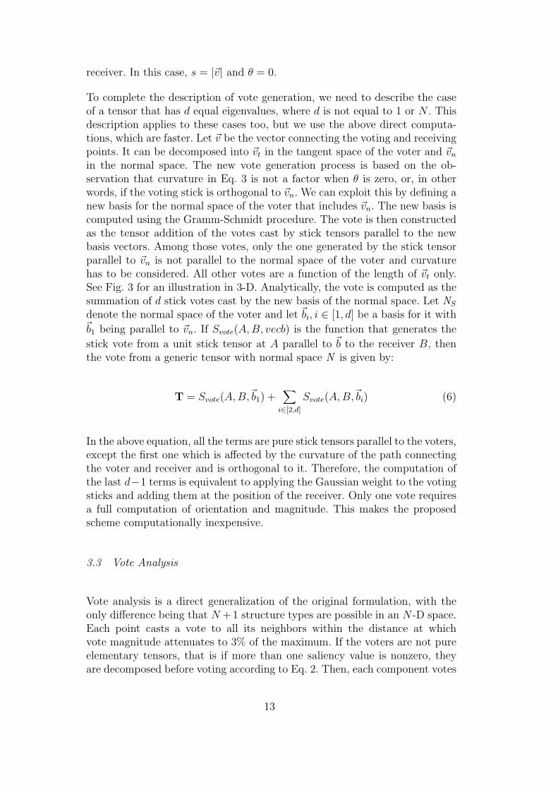
To complete the description of vote generation, we need to describe the caseof a tensor that has d equal eigenvalues, where d is not equal to 1 or N . Thisdescription applies to these cases too, but we use the above direct computa-tions, which are faster. Let ~v be the vector connecting the voting and receivingpoints. It can be decomposed into ~vt in the tangent space of the voter and ~vnin the normal space. The new vote generation process is based on the ob-servation that curvature in Eq. 3 is not a factor when θ is zero, or, in otherwords, if the voting stick is orthogonal to ~vn. We can exploit this by defining anew basis for the normal space of the voter that includes ~vn. The new basis iscomputed using the Gramm-Schmidt procedure. The vote is then constructedas the tensor addition of the votes cast by stick tensors parallel to the newbasis vectors. Among those votes, only the one generated by the stick tensorparallel to ~vn is not parallel to the normal space of the voter and curvaturehas to be considered. All other votes are a function of the length of ~vt only.See Fig. 3 for an illustration in 3-D. Analytically, the vote is computed as thesummation of d stick votes cast by the new basis of the normal space. Let NS

denote the normal space of the voter and let ~bi, i ∈ [1, d] be a basis for it with~b1 being parallel to ~vn. If Svote(A,B, vecb) is the function that generates the

stick vote from a unit stick tensor at A parallel to ~b to the receiver B, thenthe vote from a generic tensor with normal space N is given by:

T = Svote(A,B,~b1) +∑i∈[2,d]

Svote(A,B,~bi) (6)

In the above equation, all the terms are pure stick tensors parallel to the voters,except the first one which is affected by the curvature of the path connectingthe voter and receiver and is orthogonal to it. Therefore, the computation ofthe last d−1 terms is equivalent to applying the Gaussian weight to the votingsticks and adding them at the position of the receiver. Only one vote requiresa full computation of orientation and magnitude. This makes the proposedscheme computationally inexpensive.

3.3 Vote Analysis

Vote analysis is a direct generalization of the original formulation, with theonly difference being that N +1 structure types are possible in an N -D space.Each point casts a vote to all its neighbors within the distance at whichvote magnitude attenuates to 3% of the maximum. If the voters are not pureelementary tensors, that is if more than one saliency value is nonzero, theyare decomposed before voting according to Eq. 2. Then, each component votes

13

Fig. 3. Vote generation for generic tensors. The voter here is a tensor with twonormals in 3-D. The vector connecting the voter and receiver is decomposed into~vn and ~vt that lie in the normal and tangent space of the voter. A new basis thatincludes ~vn is defined for the normal space and each basis component casts a stickvote. Only the vote generated by the orientation parallel to ~vn is not parallel to thenormal space. Tensor addition of the stick votes produces the combined vote.

separately and the vote is weighted by λd − λd+1, except the ball componentwhose vote is weighted by λD.

Votes are accumulated at each point by tensor addition, which is equivalentto matrix addition. Then, the eigensystem of the resulting tensor is computedand the tensor is decomposed as in Eq. 2. The estimate of local intrinsicdimensionality is given by the maximum gap in the eigenvalues. For instance,if λ1 − λ2 is the maximum difference between two successive eigenvalues, thedominant component of the tensor is the one that has one normal. Quantitativeresults in dimensionality estimation are presented in the Section 5 and in [9].In general, if the maximum eigenvalue spread is λd−λd+1, the estimated localintrinsic dimensionality is N − d, and the manifold has d normals and N − dtangents. Moreover, the first d eigenvectors that correspond to the largesteigenvalues are the normals to the manifold, and the remaining eigenvectorsare the tangents.

4 Comparison with the Original Implementation of Tensor Voting

In this section, we compare the differences of the implementation of tensor vot-ing according to [3] and the one proposed here. They are both approximationsof the exact vote computation: the former due to the numerical integrationused in the computation of the voting fields and due to the interpolation be-tween the pre-computed samples used in the generation of votes; the latterdue to the elimination of the uncertainty component of each vote, which asa result of the integration of multiple votes. In both cases, the representa-tion is identical since storage requirements for each token are O(N2), whichis acceptable. It can be reduced with a sparse storage scheme, but that wouldincrease the necessary computations to retrieve information. The limitationof the original implementation is the generation and storage of voting fields,which is exponential with respect to the dimensionality of the space. In N -D,the storage requirements for a complete set of voting fields with k samples per

14

(a) Original implementation (b) New implementation

Fig. 4. Visualization of the ball voting field using the original and the new imple-mentation. Shown are the curve normals, as well as the tangents that representthe ball component. The ball component in the original implementation has beenexaggerated for visualization purposes, while it is zero with the new implementation.

axis, is N3 × kN , since the set contains N fields and each field has kN samplevotes which are N ×N tensors. Each of these tensors has to be computed bynumerical integration whose order ranges from 1 to N . Moreover, the likeli-hood of each pre-computed vote being used decreases with the dimensionality.Even if the votes are not pre-computed, computation via the same integrationprocess “on the fly” is also computationally expensive. The new implementa-tion is quadratic in the dimensionality of the space since it requires the directcomputation of at most N −1 stick votes for each of the N components of thevoter.

We evaluate the effectiveness of the new implementation by performing thesame experiments in 3-D using both the original and the new vote generationschemes. Figure 4 shows a cut, containing the voter, of the 3-D ball votingfield computed using the original and the new implementation. Shown arethe projections of the eigenvectors on the selected plane after voting by aball voter placed on the plane. We do not attempt to directly compare votemagnitudes, since they are defined differently. In the original implementation,the total energy of the ball field is normalized to be equal to that of the stickfield. In the new implementation, the magnitude of each ball vote is the sameas that of a stick vote cast from the voter to the receiver. This makes the totalenergy of the new field higher than that of the stick field, since there is noattenuation due to curvature at any orientation, and voting takes place at allorientations, since the 45o cut-off only applies to stick voters.

A test that captures the accuracy of the orientation conveyed by the voteis a comparison between the tangent of the ball vote and the ground truth,which should be along the line connecting the voter and receiver. Since bothimplementations are approximations, this error is non-zero. The original im-plementation is based on linear interpolation between samples computed byapproximating the integration of stick votes, while in the new implementation

15

an approximate vote is cast directly to the receiver. Both are rather accurate.The original implementation is off by 1.25× 10−5 degrees, while the new oneis off by 1.38× 10−5 degrees.

(a) Noise free (b) 2:1 outliers:inliers (c) 4:1 outliers:inliers

Fig. 5. Sphere and plane inputs used for comparing the original and new implemen-tation of tensor voting

We also compared the two implementations in a simple experiment of localstructure estimation. We sampled unoriented points from a sphere and a planein 3-D, and compared the estimated surface normals against the ground truth.Note that the coordinates of the points are quantized to make the evaluationfair for the original implementation, which only operates with integer coordi-nates due to the data structure that stores the tokens. The inputs, which areencoded as unit balls, can be seen in Fig. 5(a). Quantitative results in surfacenormal estimation are presented in Table 1.

σ2 Original TV New TV

50 2.24 1.60

100 1.47 1.18

200 1.09 0.98

500 0.87 0.93Table 1Results on the sphere and plane dataset: average error rate in degrees for normalorientation estimation using the implementation of [3] and the one proposed here.

The accuracy in surface orientation estimation is similar in both cases, witha slight edge in favor of the new implementation. The main source of inaccu-racy in the original implementation is the need for linear interpolation usingthe entries of the look-up table. It turns out that its effects on performanceare similar to those of computing an approximate vote at the exact receiverposition using the new approach. Since the difference in ball vote magnitudesbecomes important only when not all voters are ball tensors, we performed asecond pass of tensor voting using the accumulated tensors form the first passas voters. For σ2 = 100, the error was 1.31o with the original implementationand 1.20o with the new one.

16

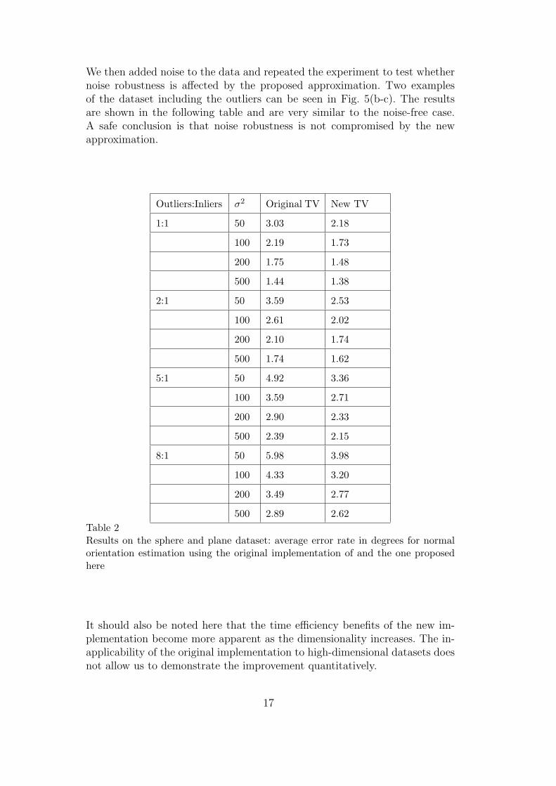
We then added noise to the data and repeated the experiment to test whethernoise robustness is affected by the proposed approximation. Two examplesof the dataset including the outliers can be seen in Fig. 5(b-c). The resultsare shown in the following table and are very similar to the noise-free case.A safe conclusion is that noise robustness is not compromised by the newapproximation.

Outliers:Inliers σ2 Original TV New TV

1:1 50 3.03 2.18

100 2.19 1.73

200 1.75 1.48

500 1.44 1.38

2:1 50 3.59 2.53

100 2.61 2.02

200 2.10 1.74

500 1.74 1.62

5:1 50 4.92 3.36

100 3.59 2.71

200 2.90 2.33

500 2.39 2.15

8:1 50 5.98 3.98

100 4.33 3.20

200 3.49 2.77

500 2.89 2.62Table 2Results on the sphere and plane dataset: average error rate in degrees for normalorientation estimation using the original implementation of and the one proposedhere

It should also be noted here that the time efficiency benefits of the new im-plementation become more apparent as the dimensionality increases. The in-applicability of the original implementation to high-dimensional datasets doesnot allow us to demonstrate the improvement quantitatively.

17

5 Dimensionality Estimation

In this section, we present experimental results in dimensionality estimation.According to Section 3.3, the intrinsic dimensionality at each point can befound as the maximum gap in the eigenvalues of the tensor after votes fromits neighboring points have been collected. All inputs consist of unorientedpoints and are encoded as ball tensors.

Fig. 6. The “Swiss Roll” dataset in 3-D

Swiss Roll The first experiment is on the “Swiss Roll” dataset, which isavailable online at http://isomap.stanford.edu/. It contains 20, 000 points ona 2-D manifold in 3-D (Fig. 6). We perform a simple evaluation of the qualityof the orientation estimates by projecting the nearest neighbors of each pointon the estimated tangent space and measuring the percentage of the distancethat has been recovered. This is a simple measure of the accuracy of the locallinear approximation of the nonlinear manifold. The percentage of points withcorrect dimensionality estimates and the percentage of recovered distancesfor the 8 nearest neighbors as a function of σ, can be seen in Table 3. Theperformance is the same at boundaries, which do not pose any additionaldifficulties to our algorithm. The number of votes cast by each point rangesfrom 187 for σ2 = 50 to 5440 for σ2 = 1000. The reported processing timesare for a Pentium 4 processor at 2.8 GHz. A conclusion that can safely bedrawn from the table is that the accuracy is high and stable for a large rangeof values of σ.

Structures with varying dimensionality The second dataset is in 4-Dand contains points sampled from three structures: a line, a 2-D cone anda 3-D hyper-sphere. The hyper-sphere is a structure with three degrees offreedom. It cannot be unfolded unless we remove a small part from it. Figure7(a) shows the first three dimensions of the data. The dataset contains a total135, 864 points, which are encoded as ball tensors. Tensor voting is performedwith σ2 = 200. Figures 7(b-d) show the points classified according to theirdimensionality. Performing the same analysis as above for the accuracy of thetangent space estimation, 91.04% of the distances of the 8 nearest neighbors of

18

σ2 Correct Dim. Perc. of Dist. Time (sec)

Estimation (%) Recovered (%)

50 99.25 93.07 7

100 99.91 93.21 13

200 99.95 93.19 30

300 99.92 93.16 47

500 99.68 93.03 79

700 99.23 92.82 112

1000 97.90 92.29 181Table 3Rate of correct dimensionality estimation and execution times as functions of σ forthe “Swiss Roll” dataset.

(a) Input (b) 1-D points

(c) 2-D points (d) 3-D points

Fig. 7. Data of varying dimensionality in 4-D. The first three axes of the input andthe classified points are shown.Note that the hyper-sphere is empty in 4-D, butappears as a full sphere when visualized in 3-D.

each point lie on the tangent space, even though both the cone and the hyper-sphere have intrinsic curvature and cannot be accurately approximated bylinear models. All the methods presented in Sec. 2 fail for this dataset becauseof the presence of structures with different dimensionalities and because thehyper-sphere cannot be unfolded.

19

Data in high dimensions The datasets for this experiment were gener-ated by sampling a few thousand points from a low-dimensional space (3- or4-D) and mapping them to a medium dimensional space (14- to 16-D) us-ing linear and quadratic functions. The generated points were then rotatedand embedded in a 50- to 150-D space, while outliers drawn from a uniformdistribution were added to the dataset. The percentage of correct point-wisedimensionality estimates after tensor voting can be seen in Table 4.

Intrinsic Linear Quadratic Space Dim.

Dim. Mappings Mappings Dim. Est. (%)

4 10 6 50 93.6

3 8 6 100 97.4

4 10 6 100 93.9

3 8 6 150 97.3Table 4Rate of correct dimensionality estimation for high dimensional data

6 Manifold Learning

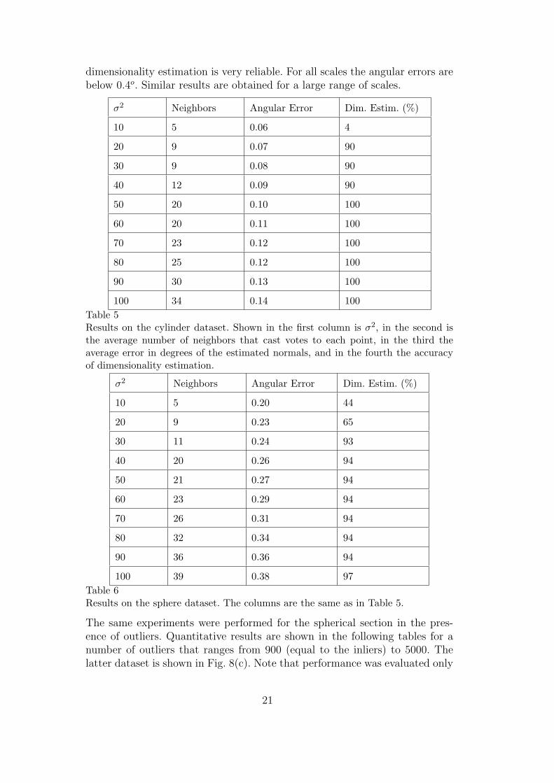
In this section, we present quantitative results on simple datasets in 3-D forwhich ground truth can be analytically computed. The two datasets are asection of a cylinder and a section of a sphere shown in Fig. 8. The cylin-drical section spans 150o and consists of 1000 points. The spherical sectionspans 90o× 90o and consists of 900 points. Both are approximately uniformlysampled. The points are represented by ball tensors, assuming no informationabout their orientation. In the first part of the experiment, we compute localdimensionality and normal orientation as a function of scale. The results arepresented in Tables 5 and 6. The results show that if the scale is not too small,

(a) Cylinder (b) Sphere (c) Noisy sphere

Fig. 8. The cylinder and sphere datasets

20

dimensionality estimation is very reliable. For all scales the angular errors arebelow 0.4o. Similar results are obtained for a large range of scales.

σ2 Neighbors Angular Error Dim. Estim. (%)

10 5 0.06 4

20 9 0.07 90

30 9 0.08 90

40 12 0.09 90

50 20 0.10 100

60 20 0.11 100

70 23 0.12 100

80 25 0.12 100

90 30 0.13 100

100 34 0.14 100Table 5Results on the cylinder dataset. Shown in the first column is σ2, in the second isthe average number of neighbors that cast votes to each point, in the third theaverage error in degrees of the estimated normals, and in the fourth the accuracyof dimensionality estimation.

σ2 Neighbors Angular Error Dim. Estim. (%)

10 5 0.20 44

20 9 0.23 65

30 11 0.24 93

40 20 0.26 94

50 21 0.27 94

60 23 0.29 94

70 26 0.31 94

80 32 0.34 94

90 36 0.36 94

100 39 0.38 97Table 6Results on the sphere dataset. The columns are the same as in Table 5.

The same experiments were performed for the spherical section in the pres-ence of outliers. Quantitative results are shown in the following tables for anumber of outliers that ranges from 900 (equal to the inliers) to 5000. Thelatter dataset is shown in Fig. 8(c). Note that performance was evaluated only

21

on the points that belong to the sphere. Larger values of the scale prove tobe more robust to noise, as expected. The smallest values of the scale resultin voting neighborhoods that include less than 10 points, which are insuffi-cient. Taking this into account, performance is still good even with wrongparameter selection. Also note that one could reject the outliers by threshold-ing, since they have smaller eigenvalues than the inliers, and perform tensorvoting again to obtain even better estimates of structure and dimensionality.Even a single pass of tensor voting, however, turns out to be very effective,especially considering that no other method can handle such a large numberof outliers. Foregoing the low-dimensional embedding is a main reason thatallows our method to perform well in the presence of noise, since embeddingrandom outliers in alow-dimensional space would make their influence moredetrimental. This is due to the structure imposed to them by the mapping,which makes the outliers less random, and due to the increase in their densityin the low-dimensional space compared to that in the original high-dimensionalspace.

Outliers 900 3000 5000

σ2

10

20

30

40

50

60

70

80

90

100

AE DE

1.15 44

0.93 65

0.88 92

0.88 93

0.90 93

0.93 94

0.97 94

1.00 94

1.04 95

1.07 97

AE DE

3.68 41

2.95 52

2.63 88

2.49 90

2.41 92

2.38 93

2.38 93

2.38 94

2.38 95

2.39 95

AE DE

6.04 39

4.73 59

4.15 85

3.85 88

3.63 91

3.50 93

3.43 93

3.38 94

3.34 94

3.31 95Table 7Results on the sphere dataset contaminated by noise. AE: error in normal angleestimation in degrees, DE: correct dimensionality estimation (%).

7 Discussion

We have presented an approach to manifold learning that offers certain ad-vantages over the state of the art. In terms of dimensionality estimation, weare able to obtain accurate estimates at the point level. Moreover, since thedimensionality is found as the maximum gap in the eigenvalues of the tensor

22

at each point, no thresholds are needed. In most other approaches, the dimen-sionality has to be provided, or, at best, an average intrinsic dimensionality isestimated for the entire dataset, as in [8, 12–14,24].

Even though tensor voting on the surface looks similar to other local, instance-based learning algorithms that propagate information from point to point,the fact that the votes are tensors and not scalars allows them to conveyconsiderably more information. The properties of the tensor representation,which can handle the simultaneous presence of multiple orientations, allow thereliable inference of the normal and tangent space at each point. In addition,tensor voting is very robust against outliers, as demonstrated for the 2-D and3-D case in numerous publications including [3, 10]. This property holds inhigher dimensions, where random noise is even more scattered.

It should also be noted that the votes attenuate with distance and curvature.This is a more intuitive formulation than using the K nearest neighbors withequal weights, since some of them may be too far, or belong to a differentpart of the structure. For both tensor voting and the methods presented inSection 2, however, the distance metric in the input space has to be mean-ingful. Our method is less sensitive to a somewhat incorrect selection of thedistance metric since all neighbors do not contribute equally. The selectionof the distance metric is discussed later in this section. After this choice hasbeen made, the only free parameter in our approach is σ, the scale of voting.Small values tend to preserve details better, while large values are more robustagainst noise. The scale can be selected automatically by randomly samplinga few points before voting and making sure that enough points are includedin their voting neighborhoods. The number of points that can be consideredsufficient is a function of the dimensionality of the space as well as the intrinsicdimensionality of the data. A full investigation of data sufficiency is amongthe objectives of our future research. Our results show that sensitivity withrespect to scale is small, as shown in Tables 3 and 5-7.

Another important advantage of tensor voting is the absence of global compu-tations, which makes time complexity O(NMlogM), whereN is the dimensionof the space and M is the number of points. This property enables us to pro-cess datasets with very large number of points. Computation time does notbecome impractical as the number of points grows, assuming that more pointsare added to the dataset in a way that the density remains constant. In thiscase, the number of votes cast per point remains constant and time require-ments grow linearly. If points are added in a way that increases the averagedensity, voting can be performed with a smaller σ, thus maintaining the num-ber of votes cast and the computation time per point. Complexity is adverselyaffected by the dimensionality of the space N , since eigen-decompositions ofN × N tensors have to be performed. For most practical purposes, however,the number of points has to be considerably larger than the dimensionality

23

of the space (M � N) to allow structure inference. Computational complex-ity, therefore, is reasonable with respect to the largest parameter, which istypically M .

The novelty of our approach to manifold learning is that it is not based ondimensionality reduction, in the form of an embedding or mapping between ahigh and a low dimensional space. Instead, we perform tasks such as geodesicdistance measurement and nonlinear interpolation in the input space. Experi-mental results show that we can perform these tasks in the presence of outliernoise at high accuracy, even without explicitly removing the outliers from thedata. This is due to the fact that the accumulated tensors at the outliers donot develop any preference for a particular structure and do not outweighthe contributions of the inliers. In addition, outlier distribution remains ran-dom, since dimensionality reduction and an embedding to a lower-dimensionalspace are not attempted. This choice also broadens the range of datasets wecan process. While isometric embeddings can be achieved for a certain class ofmanifolds, we are able to process non-flat manifolds and even non-manifolds.To the best of our knowledge, this is impossible with any other method. Ifdimensionality reduction is desired due to its considerable reduction in stor-age requirements, a dimensionality reduction method, such as [6–8,21,23,24],can be used after tensor voting. The benefits of this process are in the form ofnoise robustness and smooth component identification, with respect to bothdimensionality and orientation, via tensor voting followed by memory savingsvia dimensionality reduction.

As mentioned above, an issue we do not fully address here is that of the selec-tion of an appropriate distance metric. We assume that the Euclidean distancein the input coordinate system is a meaningful distance metric. This is not thecase if the measurements are not of the same type, as for instance distancesand angles. On the other hand, a metric such as the Mahalanobis distance isnot necessarily appropriate in all cases, since the data may lie in a subspace ofthe input space and giving equal weight to all dimensions, including the redun-dant ones, would be detrimental. For the experiments shown in this chapter,we apply heuristic scaling of the coordinates when necessary. We intend todevelop a systematic way based on cross-validation that automatically scalesthe coordinates by maximizing prediction performance for the observationsthat have been left out.

Our future research will focus on addressing the limitations of our currentalgorithm and extending its capabilities. In the area of function approximation,the issue of approximating functions with multiple branches for the same inputvalue, which often appear in practical applications, has to be handled morerigorously. In addition, an interpolation mechanism that takes into accountholes and boundaries should be implemented. We also intend to develop anonline, incremental version of our approach, possible including a forgetting and

24

an updating module, that will be able to process data as they are collected,instead of requiring the entire dataset to proceed. Potential applications of ourwork include challenging real problems, such as the study of direct and inversekinematics. One can also view the proposed approach as learning data froma single class, which can serve as groundwork for an approach for supervisedand unsupervised classification.

Acknowledgement

This research has been supported by the National Science Foundation grantIIS 03 29247. The authors would like to thank Adit Sahasrabudhe for his helpwith some of the experiments.

Appendix A: User Guide for the N-D Tensor Voting Executable

The executable reads an input file, performs tensor voting with the user-defined value for sigma2 and writes the resulting tensors to the output file.

The syntax is: VotingND infile outfile sigma2

The input file is a text file that begins with an unsigned integer that specifiesthe dimensionality of the space, followed by a list of un-oriented points ortensors, or a mixture of both. An un-oriented point is represented by its coor-dinates followed by a 0, such that a file containing un-oriented points wouldlook like this:

Nx1 1 x1 2 ... x1 N 0x2 1 x2 2 ... x2 N 0...xM 1 xM 2 ... xM N 0

Where xi are the M points and xi j, j=1..N are the coordinates of each point.The number of points does not need to be specified. The points are encodedas unit ball tensors with all eigenvalues equal to one and an orthonormal setof eigenvectors.

Alternatively, one can input points with orientation information in the formof tensors. In this case, the coordinates are followed by a 1 to indicate thatthe point is associated with a tensor. Following the 1, the input file containsthe eigenvalues of the tensor in decreasing order and then the eigenvectors

25

starting from the one corresponding to the maximum eigenvalue. The inputfile should be in the following form:

Nx1 1 x1 2 ... x1 N 1lambda1 1 lambda1 2 ... lambda1 Ne1 11 e1 12 ... e1 1N...e1 N1 e1 N2 ... e1 NN...xM 1 xM 2 .. xM N 1lambdaM 1 lambdaM 2 ... lambdaM NeM 11 eM 12 ... eM 1N...eM N1 eM N2 ... eM NN

Line feeds are actually ignored. They are included here for clarity. Also, thecode can read the 0 or 1 index in integer or floating form. If one wishes tocompute saliency values at locations that do not participate in the computa-tion, these should be associated with zero ball tensors. Such tensors have tobe provided in the second format as tensors with all eigenvalues equal to zero.

The output file is also a text file that contains the tensors accumulated aftervoting at the input positions. It is always in the second format. It can be useddirectly as input for a second pass of tensor voting, if so desired.

The final parameter is the square of the scale of the voting field which ef-fectively determines the size of the voting neighborhood and the degree ofsmoothness. The scale should be set according to the dimensions of the inputspace. A scale below 1.0 would probably result in no information propagationin a space where the average distance between points is more than 10 units oflength.

Since Euclidean distances are used when computing the magnitude of thevotes that are cast from point to point, the input coordinates may need to bescaled in a way that ensures that the Euclidean distances between points aremeaningful. This functionality is not provided since it is problem-dependent.

26

Appendix B: User License for the Approximate Nearest NeighborLibrary (ANN) (Release 0.1)

The following is the user license agreement for the Approximate Nearest Neigh-bor Library (ANN) (Release 0.1) [11] which is used to store the data in oursoftware.

“Copyright (c) 1997-1998 University of Maryland and Sunil Arya and DavidMount. All Rights Reserved.

This software and related documentation is part of the Approximate NearestNeighbor Library (ANN).

Permission to use, copy, and distribute this software and its documentation ishereby granted free of charge, provided that

(1) it is not a component of a commercial product, and(2) this notice appears in all copies of the software and related documentation.

The University of Maryland (U.M.) and the authors make no representationsabout the suitability or fitness of this software for any purpose. It is provided“as is” without express or implied warranty.”

References

[1] S. Russell, P. Norvig, Artificial Intelligence: A Modern Approach, Prentice-Hall,Englewood Cliffs, NJ, 2003.

[2] T. Mitchell, Machine Learning, McGraw-Hill, New York, 1997.

[3] G. Medioni, M. Lee, C. Tang, A Computational Framework for Segmentationand Grouping, Elsevier, New York, NY, 2000.

[4] P. Mordohai, G. Medioni, Stereo using monocular cues within the tensor votingframework, in: European Conf. on Computer Vision, 2004, pp. 588–601.

[5] B. Scholkopf, A. Smola, K.-R. Muller, Nonlinear component analysis as a kerneleigenvalue problem., Neural Computation 10 (5) (1998) 1299–1319.

[6] S. Roweis, L. Saul, Nonlinear dimensionality reduction by locally linearembedding, Science 290 (2000) 2323–2326.

[7] J. Tenenbaum, V. de Silva, J. Langford, A global geometric framework fornonlinear dimensionality reduction, Science 290 (2000) 2319–2323.

[8] M. Brand, Charting a manifold, in: Advances in Neural Information ProcessingSystems 15, MIT Press, Cambridge, MA, 2003, pp. 961–968.

27

[9] P. Mordohai, G. Medioni, Unsupervised dimensionality estimation and manifoldlearning in high-dimensional spaces by tensor voting, in: Int. Joint Conf. onArtificial Intelligence, 2005, pp. 798–803.

[10] C. Tang, G. Medioni, Inference of integrated surface, curve, and junctiondescriptions from sparse 3d data, IEEE Trans. on Pattern Analysis and MachineIntelligence 20 (11) (1998) 1206–1223.

[11] S. Arya, D. M. Mount, N. S. Netanyahu, R. Silverman, A. Y. Wu, An optimalalgorithm for approximate nearest neighbor searching, Journ. of the ACM 45(1998) 891–923.

[12] J. Bruske, G. Sommer, Intrinsic dimensionality estimation with optimallytopology preserving maps, IEEE Trans. on Pattern Analysis and MachineIntelligence 20 (5) (1998) 572–575.

[13] B. Kegl, Intrinsic dimension estimation using packing numbers, in: Advances inNeural Information Processing Systems 15, MIT Press, Cambridge, MA, 2005,pp. 681–688.

[14] J. Costa, A. Hero, Geodesic entropic graphs for dimension and entropyestimation in manifold learning, IEEE Trans. on Signal Process 52 (8) (2004)2210–2221.

[15] E. Levina, P. Bickel, Maximum likelihood estimation of intrinsic dimension, in:Advances in Neural Information Processing Systems 17, MIT Press, Cambridge,MA, 2005, pp. 777–784.

[16] I. Jolliffe, Principal Component Analysis, Springer-Verlag, New York, 1986.

[17] T. Cox, M. Cox, Multidimensional Scaling, Chapman & Hall, London, 1994.

[18] L. K. Saul, S. T. Roweis, Think globally, fit locally: unsupervised learning oflow dimensional manifolds., Journal of Machine Learning Research 4 (2003)119–155.

[19] Y. Teh, S. Roweis, Automatic alignment of local representations, in: Advances inNeural Information Processing Systems 15, MIT Press, Cambridge, MA, 2003,pp. 841–848.

[20] V. de Silva, J. Tenenbaum, Global versus local methods in nonlineardimensionality reduction, in: Advances in Neural Information ProcessingSystems 15, MIT Press, Cambridge, MA, 2003, pp. 705–712.

[21] M. Belkin, P. Niyogi, Laplacian eigenmaps for dimensionality reduction anddata representation, Neural Computation 15 (6) (2003) 1373–1396.

[22] X. He, P. Niyogi, Locality preserving projections, in: S. Thrun, L. Saul,B. Scholkopf (Eds.), Advances in Neural Information Processing Systems 16,MIT Press, Cambridge, MA, 2004.

[23] D. Donoho, C. Grimes, Hessian eigenmaps: new tools for nonlineardimensionality reduction, in: Proceedings of National Academy of Science, 2003,pp. 5591–5596.

28

[24] K. Weinberger, L. Saul, Unsupervised learning of image manifolds bysemidefinite programming, in: Proc. Int. Conf. on Computer Vision and PatternRecognition, 2004, pp. II: 988–995.

[25] J. Wang, Z. Zhang, H. Zha, Adaptive manifold learning, in: L. K. Saul, Y. Weiss,L. Bottou (Eds.), Advances in Neural Information Processing Systems 17, MITPress, Cambridge, MA, 2005.

[26] Z. Zhang, H. Zha, Principal manifolds and nonlinear dimension reduction vialocal tangent space alignment, SIAM Journal of Scientific Computing 26 (1)(2004) 313–338.

[27] G. Guy, G. Medioni, Inferring global perceptual contours from local features,Int. Journ. of Computer Vision 20 (1/2) (1996) 113–133.

[28] W. Kohler, Physical gestalten, W.D. Ellis (ed), A source book of Gestaltpsychology (1950) (1920) 17–54.

[29] M. Wertheimer, Laws of organization in perceptual forms, PsycologischeForschung, Translation by W. Ellis, A source book of Gestalt psychology (1938)4 (1923) 301–350.

[30] K. Koffka, Principles of Gestalt Psychology, Harcourt, Brace, New York, 1935.

[31] G. Guy, G. Medioni, Inference of surfaces, 3d curves, and junctions from sparse,noisy, 3d data, IEEE Trans. on Pattern Analysis and Machine Intelligence19 (11) (1997) 1265–1277.

[32] C. Tang, G. Medioni, M. Lee, N-dimensional tensor voting and application toepipolar geometry estimation, IEEE Trans. on Pattern Analysis and MachineIntelligence 23 (8) (2001) 829–844.

[33] P. Parent, S. Zucker, Trace inference, curvature consistency, and curvedetection, IEEE Trans. on Pattern Analysis and Machine Intelligence 11 (8)(1989) 823–839.

[34] E. Saund, Labeling of curvilinear structure across scales by token grouping, in:Int. Conf. on Computer Vision and Pattern Recognition, 1992, pp. 257–263.

[35] S. Sarkar, K. Boyer, A computational structure for preattentive perceptualorganization: Graphical enumeration and voting methods, IEEE Trans. onSystems, Man and Cybernetics 24 (1994) 246–267.

[36] S. Yen, L. Finkel, Extraction of perceptually salient contours by striate corticalnetworks, Vision Research 38 (5) (1998) 719–741.

29