Open Journal of Statistics, 2017, 7, 702-717 http://www.scirp.org/journal/ojs
ISSN Online: 2161-7198 ISSN Print: 2161-718X
Dimensionality Reduction of High-Dimensional Highly Correlated Multivariate Grapevine Dataset
Uday Kant Jha1, Peter Bajorski1, Ernest Fokoue1, Justine Vanden Heuvel2, Jan van Aardt1, Grant Anderson1
1Rochester Institute of Technology, Rochester, NY, USA 2School of Integrative Plant Science, Cornell University, Ithaca, NY, USA
Abstract Viticulturists traditionally have a keen interest in studying the relationship be-tween the biochemistry of grapevines’ leaves/petioles and their associated spec-tral reflectance in order to understand the fruit ripening rate, water status, nu-trient levels, and disease risk. In this paper, we implement imaging spectroscopy (hyperspectral) reflectance data, for the reflective 330 - 2510 nm wavelength re-gion (986 total spectral bands), to assess vineyard nutrient status; this constitutes a high dimensional dataset with a covariance matrix that is ill-conditioned. The identification of the variables (wavelength bands) that contribute useful informa-tion for nutrient assessment and prediction, plays a pivotal role in multivariate statistical modeling. In recent years, researchers have successfully developed many continuous, nearly unbiased, sparse and accurate variable selection methods to overcome this problem. This paper compares four regularized and one functional regression methods: Elastic Net, Multi-Step Adaptive Elastic Net, Minimax Con-cave Penalty, iterative Sure Independence Screening, and Functional Data Analy-sis for wavelength variable selection. Thereafter, the predictive performance of these regularized sparse models is enhanced using the stepwise regression. This comparative study of regression methods using a high-dimensional and highly correlated grapevine hyperspectral dataset revealed that the performance of Elas-tic Net for variable selection yields the best predictive ability.
for high-dimensional datasets. It remains a challenge to identify a small fraction of essential predictors from thousands of variables, especially for small sample sizes. Variable selection by way of a sparse approximation of the parsimonious model can enhance the prediction and estimation accuracy by efficiently identifying the subset of essential predictors, reduce model complexity and improve model inter-pretability. This paper presents some unbiased, sparse and continuous methods for the judicious selection of important predictors, which allow easier interpretation, better prediction, and reduction in the complexity of the model.
This paper utilized a hyperspectral data, collected from vines at the leaf-level and the canopy-level, for a Riesling vineyard. The dataset was obtained by mea-suring the spectral reflectance, defined as the ratio of backscattered radiance from a surface and the incident radiance on that surface (scaled to 0% - 100%) [1], directly over the leaves during the bloom period of growth. These in situ spectral measurements were coupled to the contemporaneous nutrient analysis of the petiole (leaf stem) [2], as per Wine Grape Production Guide for Eastern North America [3]. The goal of that project was to develop vineyard nutrient models (nitrogen, potassium, phosphorous, magnesium, zinc, and boron), with wavelengths in the reflective regime (approximately 350 - 2500 nm) as predictor variables, toward rapid assessment vine nutrient status using remote sensors, such as cameras mounted on Unmanned Aerial Systems (UAS). Examples of similar past studies can be found in Soil Research [4]. Such an approach would enable growers to rapidly assess vineyard nutrient needs and apply remedial management interventions, e.g., tailored fertilization regimes. However, the ap-proach is only useful if such models are accurate and precise, i.e., consistency and associated model robustness are critical. This specific grapevine dataset has n = 144 observations and p = 986 spectral bands, treated here as predictor va-riables; to reiterate, the objective was to identify those wavelengths or wave-length regions that are unbiased and precise predictors of a specific nutrient’s level in the plant. To achieve compatibility with 144 observations of predictors, six replicates of each of the response variable of 24 leaf-level spectral samples have been used.
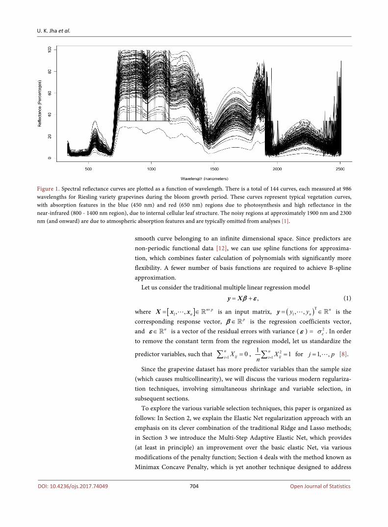
This high dimensional dataset, with more number of variables than the sample size, suffers from the curse of dimensionality, ill-posedness [5] and multicollinearity as shown in Figure 1. Hence, a thorough analysis of such data requires modern re-gularization techniques involving simultaneous shrinkage and variable selection.
One popular family of feature selection methods for parametric models is based on the penalized (pseudo-) likelihood approach. These regularization paths for Generalized Linear Models via Coordinate Descent include the Lasso [6], the Smoothly Clipped Absolute Deviation [7], the Elastic Net [8], the Minimax Concave Penalty [9], Multi-Step Adaptive Elastic Net [10], and related techniques. Fan & Lv [11] introduced Sure Independence Screening, where the sure screening is achieved by correlation learning. Since the spectral reflectance data have been measured along the continuum of wavelengths from 330 - 2510 nm, at a spectral sampling interval from 1.5 - 2.7 nm, it can be represented by a
DOI: 10.4236/ojs.2017.74049 703 Open Journal of Statistics
Figure 1. Spectral reflectance curves are plotted as a function of wavelength. There is a total of 144 curves, each measured at 986 wavelengths for Riesling variety grapevines during the bloom growth period. These curves represent typical vegetation curves, with absorption features in the blue (450 nm) and red (650 nm) regions due to photosynthesis and high reflectance in the near-infrared (800 - 1400 nm region), due to internal cellular leaf structure. The noisy regions at approximately 1900 nm and 2300 nm (and onward) are due to atmospheric absorption features and are typically omitted from analyses [1].
smooth curve belonging to an infinite dimensional space. Since predictors are non-periodic functional data [12], we can use spline functions for approxima-tion, which combines faster calculation of polynomials with significantly more flexibility. A fewer number of basis functions are required to achieve B-spline approximation.
Let us consider the traditional multiple linear regression model
,= +y Xβ ε (1)
where [ ]1, , n pn
×= ∈X x x is an input matrix, ( )T1, , n
ny y= ∈y is the corresponding response vector, p∈β is the regression coefficients vector, and n∈ε is a vector of the residual errors with variance ( ε ) = 2
εσ . In order to remove the constant term from the regression model, let us standardize the
predictor variables, such that 1 0niji X
==∑ , 2
1
1 1
niji X
n ==∑ for 1, ,j p= [8].
Since the grapevine dataset has more predictor variables than the sample size (which causes multicollinearity), we will discuss the various modern regulariza-tion techniques, involving simultaneous shrinkage and variable selection, in subsequent sections.
To explore the various variable selection techniques, this paper is organized as follows: In Section 2, we explain the Elastic Net regularization approach with an emphasis on its clever combination of the traditional Ridge and Lasso methods; in Section 3 we introduce the Multi-Step Adaptive Elastic Net, which provides (at least in principle) an improvement over the basic elastic Net, via various modifications of the penalty function; Section 4 deals with the method known as Minimax Concave Penalty, which is yet another technique designed to address
DOI: 10.4236/ojs.2017.74049 704 Open Journal of Statistics
the estimation, inference and prediction inherent in complex datasets, like the grapevine data studied in this paper; in Section 5 we discuss various aspects of iterative Sure Independence Screening; Section 6 adopts a conceptually different approach, by using a functional approach to variable selection, including smoothing by basis representation and validation; Section 7 is dedicated to the comparative analysis of the performance of all of the above techniques with the goal of wavelength selection for the Riesling grapevine dataset toward nutrient estimation; and finally, in Section 8, we discuss the advantages and limitations of the various models mentioned above before concluding.
2. Elastic Net
Ridge regression, the oldest and earliest form of regularization, shrinks all coef-ficients of the predictors towards zero by a uniform (ℓ2 – norm) convex penalty to produce a unique solution. However, Ridge regression typically does not set the coefficients exactly to zero, unless λ = ∞ [6]. Indeed, for the scientific prob-lem underlying the grapevine data, it is important to achieve both shrinkage and variable selection. Hence, Ridge regression is not suitable for the high dimen-sional grapevine dataset. The Ridge regression coefficients are defined as
( ) { }2 2Ridge2 2
ˆ arg min pββ λ
∈= − +y X
β β
(2)
where ( )22 T12 n
i ii y β=
− = −∑y xXβ is a quadratic loss function (residual sum of squares), T
ix is the ith row of X, 2 212 p
jj β=
=∑β is the ℓ2–norm penalty on β , and 0λ ≥ is the tuning (penalty) parameter, which regulates the strength of the penalty.
Lasso, on the other hand, shrinks all coefficients by a constant value (ℓ1 - norm) and typically sets some of them to zero for some appropriately chosen λ. It simultaneously achieves continuous shrinkage and automatic variable selec-tion. However, when the multicollinearity is very high, Lasso tends to pick one of the predictors from the cluster in an arbitrary way and then shrink the others to zero [8]. The grapevine data are highly correlated; the arbitrariness of variable selection, therefore, will yield multiple solutions. Hence, analysis of the grape-vine dataset using Lasso may not always yield a unique solution, as needed. The Lasso regression coefficients are defined as
( ) { }2Lasso2 1
ˆ arg min pββ λ
∈= − +Xy
β β (3)
where ( )22 T12
1 2
ni ii y
nβ
=− = −∑y X xβ is the quadratic loss function, T
ix is
the ith row of the matrix X, 11 p
jj β=
=∑β is the ℓ1–norm penalty on β ,
which induces sparsity in the solution, and 0λ ≥ is the tuning parameter. Naïve Elastic Net (NEN) overcomes these limitations by combining of the
Lasso (ℓ1-norm) and Ridge (ℓ2-norm) penalties [8]. Let us consider two fixed non-negative tuning parameters: λ1 and λ2, such that
the naïve elastic net criterion is
DOI: 10.4236/ojs.2017.74049 705 Open Journal of Statistics
The NEN estimator ( )N-Enetβ̂ is the minimizer of equation [8]: ( ) ( ){ }N-Enet
1 2ˆ arg min , ,
pL
ββ λ λ
∈=
β (5)
Let us consider ( )2 1 2α λ λ λ= + , then the elastic net estimator ( )N-enetβ̂ is ( ) ( ){ }2N-Enet
2ˆ arg min
pPα
ββ λ
∈= − +y X
β β
(6)
subject to ( ) ( ) 2
2 11P tα α α= − + ≤β β β for some t. where ( )Pα β is the naïve elastic net penalty and ( )0,1α ∈ . For all ( )0,1α ∈ , the penalty function is non-differentiable at 0 (like Lasso) but strictly convex (like ridge). Hence, by varying α, we can control the proportion of ℓ1-norm (α = 0) and the ℓ2-norm (α = 1) penalty. The amount of shrinkage to coefficient estimates is controlled by the parameter t ≥ 0.
Initially, the NEN computes the ridge regression coefficients for each fixed tuning parameter λ2 and then uses this coefficient value to acquire shrinkage along the Lasso coefficient paths. This technique of shrinkage increases the bias of the coefficients without substantial reduction in the variance, resulting in an overall increase of the prediction error. This leads to a doubled shrinkage and unnecessary extra bias, in comparison to Ridge regression or Lasso [8]. Elastic Net
can correct this double shrinkage by multiplying the NEN estimate by 21nλ +
:
( ) { }2 2Enet 21 22 1 2
ˆ 1 arg minpn β
λβ λ λ
∈
= + − + +
y X
β β β (7)
This type of transformation reverts to ridge shrinkage while retaining the va-riable selection property of the NEN. Thus, the elastic net is able to improve the prediction accuracy by achieving the automatic variable selection using ℓ1 pe-nalty, while group selection and stabilization of the coefficient paths on random sampling are achieved by ℓ2 penalty. The sparsity of the elastic net increases monotonically from zero to the sparsity of the Lasso solution as α increases from 0 to 1, for a given parameter λ. Hence, the Elastic Net is a better solution for a dataset with a sample size significantly smaller than the number of highly corre-lated predictors [13].
At times, it is advisable to include the entire group of correlated predictors in the model selection, rather than single variable from the group. In such cases, elastic net ensures that the highly correlated variables enter or exit the model together. The presence of the ℓ2-norm ensures a unique minimum by making the loss function strictly convex [8].
3. Multi-Step Adaptive Elastic Net
Lasso and elastic-net approaches result in a substantial number of non-zero
DOI: 10.4236/ojs.2017.74049 706 Open Journal of Statistics
coefficients with asymptotically non-ignorable bias. The estimation bias of the Lasso can be reduced by choosing the weights such that the variables with larger coefficients have smaller weights than variables with smaller coefficients. To mi-tigate this bias, the adaptive Lasso uses the weighted penalty approach as given below:
( ) { }2AdaLasso12
ˆ ˆarg minp
pj jj w
ββ λ β
=∈
= − + ∑Xy
β
(8)
where ˆ jw is a weighting parameter calculated from the data, ˆˆ inij jw
γβ
− =
,
and γ is a positive constant. ˆ inijβ are the initial parameters, obtained by ridge
regression or least squares. This approach ensures that the adaptive lasso is able to accomplish more
shrinkage, resulting in smaller coefficients. In other words, it executes a varying amount of shrinkage for different variables. Adaptive elastic net is a mixture of the adaptive Lasso and the elastic net. Before calculating the adaptive weights, we estimate the elastic-net ( )Enetβ̂ , and use a positive constant γ. Using this infor-mation, we can calculate adaptive weights:
( )enetˆˆ , 1, 2, ,j jw j pγ
β− = =
(9)
Now we can estimate the adaptive elastic net by the equation below:
( ) { }2 2AdaEnet 21 212 2
ˆ ˆ1 arg minp
pj jj w
n β
λβ λ β λ
=∈
= + − + +
∑Xy
β β (10)
The presence of the ℓ2-norm ensures that the adaptive elastic net is able to overcome the collinearity problem while retaining the consistency in variable selection and asymptotic Gaussian properties of the adaptive Lasso. The use of multi-step estimation achieves higher true positives (true zeroes are estimated as zeroes) for the variable selection by pursuing more iterative steps and using sep-arate tuning parameters for each step. The estimates of multi-step adaptive elas-tic net (MSA-Enet) approach are given by:
( ) ( ) ( ) ( ){ }2 2MSAEnet 121 212 2
ˆ ˆ1 arg min ?p
pk k kj jj w
n β
λβ λ β λ−
=∈
= + − + +
∑y X
β β
(11)
where k = number of iterations (stages). For MSA-Enet, we use k ≥ 3. By considering k = 2, we can estimate the adaptive elastic net, and for k = 1, we ob-tain the normal elastic-net. We can obtain the values of ( )
1kλ and ( )
2kλ by us-
ing cross-validation.
4. Minimax Concave Penalty
Convex penalties fail to satisfy all three conditions of sparsity, continuity, and unbiasedness. Hence, they cannot produce true parsimonious models. To over-come these limitations, Fan & Li [7], [14] and Zhang [9] introduced new statis-tical modeling techniques for variable selection based on nonconvex penalties, called Smoothly Clipped Absolute Deviation (SCAD) and Minimax Concave
DOI: 10.4236/ojs.2017.74049 707 Open Journal of Statistics
Penalty (MCP), respectively. However, using non-convex penalties for sparsity will yield multiple local minima of the penalized residual sum of squares, with-out any knowledge about the best estimator. Hence, the authors of SCAD and MCP regression models have emphasized the oracle property of these nonconvex penalties. The Oracle property means selection of the correct subset of predictors and estimation of the non-zero parameters as if the information were known ahead of time, based on some previous investigations and expe-riences. These nonconvex penalties are initiated at the origin as the ℓ1 penalty (Lasso) until, |x| = λ, and then smoothly relax the penalization rate to zero as the absolute value of the coefficient increases, but differs in the way that the transition takes place. The MCP relaxes the penalization rate immediately, whereas, for the SCAD, the penalization rate remains flat for a while, before de-creasing.
Zhang [9] defined MCP on [0, ∞) by
( ) | |
0; 1 d
t xt xρ λ λγλ +
= −
∫ ,
( )
2
2
, if ,2;
, if ,2
tt tt
t
λ λγγρ λ
λ γλγ
− ≤=
>
( ), if ,
;0, if ,
t tt
t
λ λγρ λ γ
λγ
− ≤′ = >
(12)
for γ > 0 and λ > 0. Equation (12) clearly shows that MCP initially applies the ℓ1 penalty (Lasso), but continuously relaxes that penalization rate until, when t > λγ. At this stage, the rate of penalization drops to 0.
MCP minimizes the maximum concavity
( ) ( ) ( ) ( ){ } ( )1 20 1 2 2 1; sup ; ;t t t t t tκ ρ κ ρ λ ρ λ ρ λ< <≡ ≡ − − (13)
subject to the following unbiasedness and features selection:
( ) ( ); 0, , 0 ;t tρ λ γλ ρ λ λ= ∀ ≥ + = (14)
The MCP achieves ( ); 1κ ρ λ γ= . A higher value of regularization parameter 𝛾𝛾 ensures reduction in unbiasedness and increase in concavity. According to [14], the penalized regression problem using the MCP function is given as:
( ) ( )2MCP2
1ˆ arg min ;2p
Pγβ
β λ∈
= − +
y X
β β (15)
where ( ) ( )1; ;pjjP pγ γλ β λ
== ∑β . Estimation of the coefficients using MCP de-
pends on the selection of the parameters γ and λ, obtained through cross-validation. For each penalty value of λ > 0, MCP offers a continuum of penalties starting with the ℓ1-norm at γ → ∞ and the ℓ0-norm as γ → 0+ [9]. Selection of γ deter-mines the sparsity of the model.
DOI: 10.4236/ojs.2017.74049 708 Open Journal of Statistics
The convexity of penalties guarantees that the coordinate descent converges to a unique global minimum and β̂ is continuous with respect to λ. Convexity ensures good starting values, which in turn, reduces the number of iterations. However, when convexity fails to exist, then β̂ may not necessarily be conti-nuous. In other words, a slight variation in the data may significantly change the coefficient estimate. The estimates obtained using non-convex penalty generally have a large variance. Although the unbiasedness and variable selection preclude convex penalties, the MCP provides the sparse convexity to the broadest extent by minimizing the maximum concavity.
For the high-dimensional grapevine dataset, global convexity is neither possible nor relevant. However, the objective function of the grapevine dataset is convex in the local region. The parsimonious solutions of this objective function have smooth coefficient paths with stable coefficients. The tuning parameter gamma ( 3γ = ) for the MCP controls how fast the penalization rate goes to zero.
5. Sure Independence Screening (SIS)
The coordinate descent algorithm (penalized likelihood) methods fail to conform to the concurrent expectations of computational expediency, statistical accuracy, and algorithmic stability in the extremely high dimensional dataset. In order to overcome this constraint, Fan & Lv [11] proposed the concept of the sure screening method, based on a component-wise regression that tackles the challenges above. Variable selection through coefficient estimates generally overfits the model; hence, authors utilized the marginal correlations, instead of regression estimates, in order to address the problem of the dimensionality re-duction of ultra high dimensional datasets. Since screening does not require in-version of a matrix, this method seems computationally attractive. This correlation screening, called Sure Independence Screening (SIS), relies on the intuition that the predictors are independent and normally distributed. In other words, each variable is independently used as a predictor to decide its usefulness in predicting the response variable.
According to Saldana & Feng [15], SIS is a two-stage procedure. It first re-moves the variables with weak marginal correlation with the response, thus achieving dimensionality reduction p below the sample size n. Then it accom-plishes variable selection and parameter estimation simultaneously through a lower dimensional penalized least squares approach, like SCAD or Lasso. Under certain regularity conditions, the independent, sure screening process keeps all of the relevant predictors in the model with a probability approaching one.
Let X be a matrix with dimension n × p and ( )T1, , pω ω= ω be a p-vector
of marginal correlations of predictors with the response variable, acquired by component-wise regression, such that
T= X yω (16)
We standardize the matrix X column-wise and rescale vector ω by the standard deviation of the response.
DOI: 10.4236/ojs.2017.74049 709 Open Journal of Statistics
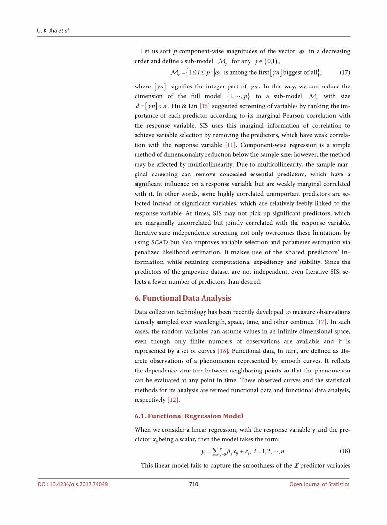
Let us sort p component-wise magnitudes of the vector ω in a decreasing order and define a sub-model γ for any ( )0,1γ ∈ ,
[ ]{ }is among the first biggest of l: , a1 li ni pγ γω= ≤ ≤ (17)
where [ ]nγ signifies the integer part of nγ . In this way, we can reduce the dimension of the full model { }1, , p to a sub-model γ with size
[ ]d n nγ= < . Hu & Lin [16] suggested screening of variables by ranking the im-portance of each predictor according to its marginal Pearson correlation with the response variable. SIS uses this marginal information of correlation to achieve variable selection by removing the predictors, which have weak correla-tion with the response variable [11]. Component-wise regression is a simple method of dimensionality reduction below the sample size; however, the method may be affected by multicollinearity. Due to multicollinearity, the sample mar-ginal screening can remove concealed essential predictors, which have a significant influence on a response variable but are weakly marginal correlated with it. In other words, some highly correlated unimportant predictors are se-lected instead of significant variables, which are relatively feebly linked to the response variable. At times, SIS may not pick up significant predictors, which are marginally uncorrelated but jointly correlated with the response variable. Iterative sure independence screening not only overcomes these limitations by using SCAD but also improves variable selection and parameter estimation via penalized likelihood estimation. It makes use of the shared predictors’ in-formation while retaining computational expediency and stability. Since the predictors of the grapevine dataset are not independent, even Iterative SIS, se-lects a fewer number of predictors than desired.
6. Functional Data Analysis
Data collection technology has been recently developed to measure observations densely sampled over wavelength, space, time, and other continua [17]. In such cases, the random variables can assume values in an infinite dimensional space, even though only finite numbers of observations are available and it is represented by a set of curves [18]. Functional data, in turn, are defined as dis-crete observations of a phenomenon represented by smooth curves. It reflects the dependence structure between neighboring points so that the phenomenon can be evaluated at any point in time. These observed curves and the statistical methods for its analysis are termed functional data and functional data analysis, respectively [12].
6.1. Functional Regression Model
When we consider a linear regression, with the response variable y and the pre-dictor xij being a scalar, then the model takes the form:
0 , 1, 2, ,pi j ij ij i ny xβ ε
== + =∑
(18)
This linear model fails to capture the smoothness of the X predictor variables
DOI: 10.4236/ojs.2017.74049 710 Open Journal of Statistics
with respect to the wavelength. However, if we replace at least one vector of pre-dictor variable observations ( )1, ,i i ipx x=x in the linear equation by a func-tional predictor xi(t), we obtain a model consisting of an intercept term along with a single functional predictor variable [17].
Let 1, , qt t be a set of times, then we can discretize each of the n functional predictors xi(t) on this set. Now fit the model:
( )0 0q
i i j j ijy x tα β ε=
= + +∑ (19)
If the refinement of the selected time is continued, then the summation will approach an integral equation, and we will get a functional linear regression model for the scalar response:
( ) ( ) ( )02, 1, , ~ ,d ;i i i ii ny x t yt t Nα µ σβ ε+ == + ∫
(20)
where the functional regression tries to establish a relationship between a scalar outcome yi and random functions xi(t) [17].
Here the constant 0α is the intercept term that adjusts for the origin of the response variable. The parameter β is in the infinitely dimensional space of ℓ2 functions (the Hilbert space of all square integral functions over a particular in-terval) [19].
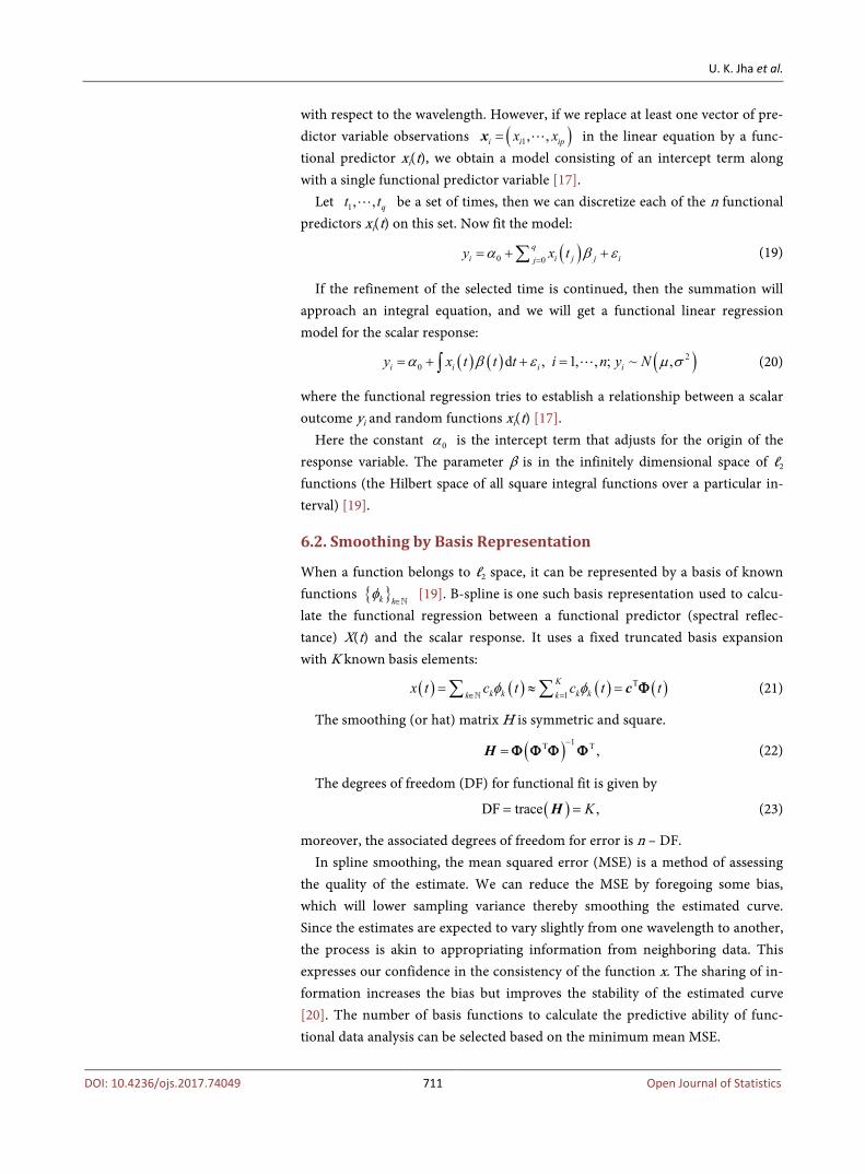
6.2. Smoothing by Basis Representation
When a function belongs to ℓ2 space, it can be represented by a basis of known functions { }k k
φ∈
[19]. B-spline is one such basis representation used to calcu-late the functional regression between a functional predictor (spectral reflec-tance) X(t) and the scalar response. It uses a fixed truncated basis expansion with K known basis elements:
( ) ( ) ( ) ( )T1
Kk k k kk kx t c t c t tφ φ
∈ == ≈ =∑ ∑ c
Φ (21)
The smoothing (or hat) matrix H is symmetric and square.
( ) 1T T ,−
=H Φ Φ Φ Φ (22)
The degrees of freedom (DF) for functional fit is given by
( )DF trace ,K= =H (23)
moreover, the associated degrees of freedom for error is n – DF. In spline smoothing, the mean squared error (MSE) is a method of assessing
the quality of the estimate. We can reduce the MSE by foregoing some bias, which will lower sampling variance thereby smoothing the estimated curve. Since the estimates are expected to vary slightly from one wavelength to another, the process is akin to appropriating information from neighboring data. This expresses our confidence in the consistency of the function x. The sharing of in-formation increases the bias but improves the stability of the estimated curve [20]. The number of basis functions to calculate the predictive ability of func-tional data analysis can be selected based on the minimum mean MSE.
DOI: 10.4236/ojs.2017.74049 711 Open Journal of Statistics
The functional approach of smoothing data performs well only when the number K of basis functions is significantly small as compared to the number of observations. Higher values of K will tend to overfit or undersmooth the data [21].
7. Comparative Study for Wavelength Selection
A proper choice of selection methods, applied under appropriate conditions, helps to build consistent parsimonious models and estimate coefficients simul-taneously for better prediction accuracy.
Here, we compare four regularized and one functional regression methods: elastic net, multi-step adaptive elastic net, minimax concave penalty, sure inde-pendence screening, and functional data analysis based on their predictive per-formance. To select the significant variables using regularized path elastic-net, multi-step adaptive elastic net, minimax concave penalty, and sure independence screening, R packages glmnet, msaenet, ncvreg, and SIS, respectively, have been used. Thereafter the predictive performance has been enhanced using stepwise re-gression. Functional regression is performed using R package “fda.usc”.
Figure 2 and Figure 3 demonstrate that the best values for the adjusted and predicted R-squared metrics, for all the six nutrients of the highly correlated grapevine data, are achieved using the generalized linear model with elastic net penalty (penalized maximum likelihood). Multi-step adaptive elastic net, which applies data-driven weights to the ℓ1 penalty of the elastic net, reduces the values of adjusted and predicted R-squared, thereby contradicting Xiao & Xu [10]. The other three methods have mixed results for the various nutrients of the
Figure 2. The adjusted R-squared value of the six nutrients measured using Elastic Net, Multi-Step Adaptive Elastic Net, Minimax Concave Penalty, iterative Sure Independence Screening, and Functional Data Analysis.
DOI: 10.4236/ojs.2017.74049 712 Open Journal of Statistics
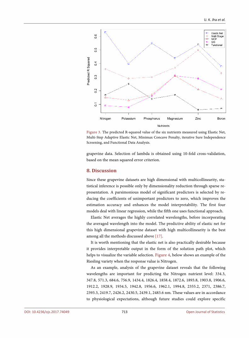
Figure 3. The predicted R-squared value of the six nutrients measured using Elastic Net, Multi-Step Adaptive Elastic Net, Minimax Concave Penalty, iterative Sure Independence Screening, and Functional Data Analysis.
grapevine data. Selection of lambda is obtained using 10-fold cross-validation, based on the mean squared error criterion.
8. Discussion
Since these grapevine datasets are high dimensional with multicollinearity, sta-tistical inference is possible only by dimensionality reduction through sparse re-presentation. A parsimonious model of significant predictors is selected by re-ducing the coefficients of unimportant predictors to zero, which improves the estimation accuracy and enhances the model interpretability. The first four models deal with linear regression, while the fifth one uses functional approach.
Elastic Net averages the highly correlated wavelengths, before incorporating the averaged wavelength into the model. The predictive ability of elastic net for this high dimensional grapevine dataset with high multicollinearity is the best among all the methods discussed above [17].
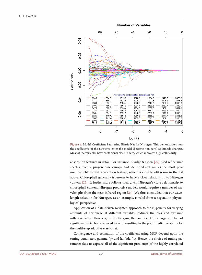
It is worth mentioning that the elastic net is also practically desirable because it provides interpretable output in the form of the solution path plot, which helps to visualize the variable selection. Figure 4, below shows an example of the Riesling variety when the response value is Nitrogen.
As an example, analysis of the grapevine dataset reveals that the following wavelengths are important for predicting the Nitrogen nutrient level: 334.3, 347.8, 571.3, 684.6, 756.9, 1434.4, 1826.4, 1858.4, 1872.6, 1893.8, 1903.8, 1906.6, 1912.2, 1928.9, 1934.5, 1942.8, 1956.6, 1962.1, 1994.8, 2355.2, 2371, 2386.7, 2393.3, 2419.7, 2426.2, 2430.5, 2439.1, 2483.6 nm. These values are in accordance to physiological expectations, although future studies could explore specific
DOI: 10.4236/ojs.2017.74049 713 Open Journal of Statistics
Figure 4. Model Coefficient Path using Elastic Net for Nitrogen. This demonstrates how the coefficients of the nutrients enter the model (become non-zero) as lambda changes. Most of the variables have coefficients close to zero, which indicates high collinearity.
absorption features in detail. For instance, Elvidge & Chen [22] used reflectance spectra from a pinyon pine canopy and identified 674 nm as the most pro-nounced chlorophyll absorption feature, which is close to 684.6 nm in the list above. Chlorophyll generally is known to have a close relationship to Nitrogen content [23]. It furthermore follows that, given Nitrogen’s close relationship to chlorophyll content, Nitrogen predictive models would require a number of wa-velengths from the near-infrared region [24]. We thus concluded that our wave-length selection for Nitrogen, as an example, is valid from a vegetation physio-logical perspective.
Application of a data-driven weighted approach to the ℓ1-penalty for varying amounts of shrinkage at different variables reduces the bias and variance inflation factor. However, in the bargain, the coefficient of a large number of significant variables is reduced to zero, resulting in the poor predictive ability for the multi-step adaptive elastic net.
Convergence and estimation of the coefficient using MCP depend upon the tuning parameters gamma (γ) and lambda (λ). Hence, the choice of tuning pa-rameter fails to capture all of the significant predictors of the highly correlated
DOI: 10.4236/ojs.2017.74049 714 Open Journal of Statistics
grapevine dataset, resulting in poor predictive ability. Sure Independence Screening, based on component-wise regression or equi-
valently correlation learning, is computationally attractive because this approach does not require matrix inversion. However, SIS is known to select unimportant predictors, which are highly correlated with the important predictors, instead of significant predictors, which are weakly related to the response. Hence, the pre-dictive performance of SIS is adversely affected in the presence of multicolli-nearity.
The functional approach of smoothing data performs well only when the number K of basis functions is significantly small as compared to the number of observations. The presence of multicollinearity fails to reduce the number of ba-sis functions significantly, based on minimum MSE, which negatively affects the predictive ability of grapevine dataset based on functional data analysis.
9. Conclusion
There has been a continuous endeavor to enhance the predictive ability of the high dimensional data by refining the coefficient estimates. These modern varia-ble selection techniques generate a sparse model, based on the assumption that the predictor variables are independent. These models yield extremely good pre-dictive accuracy when the assumption of independence is satisfied. However, for a dataset like these hyperspectral reflectance grapevine data, which is highly cor-related with a large number of predictors (wavelengths), clustered together, only Elastic Net has the ability to select the groups of correlated variables. This out-come is especially critical to the burgeoning field of precision agriculture, which is making increasing use of such hyperspectral imaging datasets but cannot reach a large sample size through traditional field work (time and monetary constraints). These data are also highly correlated (~97%). In all such cases, the predictive ability of Elastic Net is likely to outperform the other modern variable selection techniques.
Acknowledgements
We are grateful to Dr. Justine Vanden Heuvel (Cornell University) for her ex-pertise in vineyard physiology, as well as the field teams from Rochester Institute of Technology and Cornell University for their help in collecting field data.
References [1] Schott, J.R. (2007) Remote Sensing: The Image Chain Approach. Oxford University
Press, Oxford, New York.
[2] Anderson, G., van Aardt, J., Bajorski, P. and Heuvel, J.V. (2016) Detection of Wine Grape Nutrient Levels Using Visible and Near Infrared 1nm Spectral Resolution Remote Sensing. Paper Presented at the SPIE Commercial+ Scientific Sensing and Imaging.
[3] Wolf, T.K. (2008) Wine Grape Production Guide for Eastern North America. Plant and Life Sciences Publishing, Ithaca, New York, 141-142.
DOI: 10.4236/ojs.2017.74049 715 Open Journal of Statistics
[4] Shao, Y. and He, Y. (2011) Nitrogen, Phosphorus, and Potassium Prediction in Soils, Using Infrared Spectroscopy. Soil Research, 49, 166-172. https://doi.org/10.1071/SR10098
[5] Wu, P.-S. and Müller, H.-G. (2010) Functional Embedding for the Classification of Gene Expression Profiles. Bioinformatics, 26, 509-517. https://doi.org/10.1093/bioinformatics/btp711
[6] Tibshirani, R. (1996) Regression Shrinkage and Selection via the Lasso. Journal of the Royal Statistical Society. Series B (Methodological), 267-288.
[7] Fan, J. and Li, R. (2001) Variable Selection via Nonconcave Penalized Likelihood and Its Oracle Properties. Journal of the American Statistical Association, 96, 1348-1360. https://doi.org/10.1198/016214501753382273
[8] Zou, H. and Hastie, T. (2005) Regularization and Variable Selection via the Elastic net. Journal of the Royal Statistical Society: Series B (Statistical Methodology), 67, 301-320. https://doi.org/10.1111/j.1467-9868.2005.00503.x
[9] Zhang, C.-H. (2010) Nearly Unbiased Variable Selection under Minimax Concave Penalty. The Annals of Statistics, 38, 894-942. https://doi.org/10.1214/09-AOS729
[10] Xiao, N. and Xu, Q.-S. (2015) Multi-Step Adaptive Elastic Net: Reducing False Posi-tives in High-Dimensional Variable Selection. Journal of Statistical Computation and Simulation, 85, 3755-3765. https://doi.org/10.1080/00949655.2015.1016944
[11] Fan, J. and Lv, J. (2008) Sure Independence Screening for Ultrahigh Dimensional Feature Space. Journal of the Royal Statistical Society: Series B (Statistical Metho-dology), 70, 849-911. https://doi.org/10.1111/j.1467-9868.2008.00674.x
[12] Ramsay, J.O. and Dalzell, C. (1991) Some Tools for Functional Data Analysis. Jour-nal of the Royal Statistical Society. Series B (Methodological), 539-572.
[13] Schulz-Streeck, T., Ogutu, J. and Piepho, H.-P. (2012) Genomic Selection Using Regularized Linear Regression Models: Ridge Regression, Lasso, Elastic Net and Their Extensions. Proceedings of the 15th European workshop on QTL Mapping and Marker Assisted Selection (QTLMAS), 6, S10.
[14] Fan, J. and Lv, J. (2010) A Selective Overview of Variable Selection in High Dimen-sional Feature Space. Statistica Sinica, 20, 101.
[15] Saldana, D.F. and Feng, Y. (2016) SIS: An R Package for Sure Independence Screening in Ultrahigh Dimensional Statistical Models. Journal of Statistical Soft-ware, VV.
[16] Hu, Q. and Lin, L. (2017) Conditional Sure Independence Screening by Conditional Marginal Empirical Likelihood. Annals of the Institute of Statistical Mathematics, 69, 63-96. https://doi.org/10.1007/s10463-015-0534-9
[17] Jha, U.K. (2017) High-Dimensional Linear and Functional Analysis of Multivariate Grapevine Data. MS Thesis, Rochester Institute of Technology, Rochester.
[18] Jacques, J. and Preda, C. (2014) Functional Data Clustering: A Survey. Advances in Data Analysis and Classification, 8, 231-255. https://doi.org/10.1007/s11634-013-0158-y
[19] Febrero-Bande, M. and Oviedo de la Fuente, M. (2012) Statistical Computing in Functional Data Analysis: The R Package fda usc. Journal of Statistical Software, 51, 1-28. https://doi.org/10.18637/jss.v051.i04
[20] Ramsay, J. and Silverman, B. (2005) Functional Data Analysis. Springer Science & Business Media, Berlin/Heidelberg. https://doi.org/10.1002/0470013192.bsa239
[21] Ramsay, J.O., Hooker, G. and Graves, S. (2009) Functional Data Analysis with R and MATLAB. Springer Science & Business Media, Berlin/Heidelberg.
DOI: 10.4236/ojs.2017.74049 716 Open Journal of Statistics
[22] Elvidge, C.D. and Chen, Z. (1995) Comparison of Broadband and Narrow-Band Red and Near-Infrared Vegetation Indices. Remote Sensing of Environment, 54, 38-48. https://doi.org/10.1016/0034-4257(95)00132-K
[23] Hunt, E.R., Doraiswamy, P.C., McMurtrey, J.E., Daughtry, C.S., Perry, E.M. and Akhmedov, B. (2013) A Visible Band Index for Remote Sensing Leaf Chlorophyll Content at the Canopy Scale. International Journal of Applied Earth Observation and Geoinformation, 21, 103-112. https://doi.org/10.1016/j.jag.2012.07.020
Submit or recommend next manuscript to SCIRP and we will provide best service for you:
Accepting pre-submission inquiries through Email, Facebook, LinkedIn, Twitter, etc. A wide selection of journals (inclusive of 9 subjects, more than 200 journals) Providing 24-hour high-quality service User-friendly online submission system Fair and swift peer-review system Efficient typesetting and proofreading procedure Display of the result of downloads and visits, as well as the number of cited articles Maximum dissemination of your research work
Submit your manuscript at: http://papersubmission.scirp.org/ Or contact [email protected]
DOI: 10.4236/ojs.2017.74049 717 Open Journal of Statistics