Dimensionality Reduction of Multimodal Labeled Data by Local ...

Journal of Machine Learning Research 8 (2007) 1027-1061 Submitted 3/06; Revised 12/06; Published 5/07

Dimensionality Reduction of Multimodal Labeled Databy Local Fisher Discriminant Analysis∗

Masashi Sugiyama [email protected]

Department of Computer ScienceTokyo Institute of Technology2-12-1, O-okayama, Meguro-ku, Tokyo, 152-8552, Japan

Editor: Sam Roweis

AbstractReducing the dimensionality of data without losing intrinsic information is an important prepro-cessing step in high-dimensional data analysis. Fisher discriminant analysis (FDA) is a traditionaltechnique for supervised dimensionality reduction, but it tends to give undesired results if sam-ples in a class are multimodal. An unsupervised dimensionality reduction method called locality-preserving projection (LPP) can work well with multimodal data due to its locality preservingproperty. However, since LPP does not take the label information into account, it is not necessarilyuseful in supervised learning scenarios. In this paper, we propose a new linear supervised dimen-sionality reduction method called local Fisher discriminant analysis (LFDA), which effectivelycombines the ideas of FDA and LPP. LFDA has an analytic form of the embedding transformationand the solution can be easily computed just by solving a generalized eigenvalue problem. Wedemonstrate the practical usefulness and high scalability of the LFDA method in data visualiza-tion and classification tasks through extensive simulation studies. We also show that LFDA can beextended to non-linear dimensionality reduction scenarios by applying the kernel trick.Keywords: dimensionality reduction, supervised learning, Fisher discriminant analysis, localitypreserving projection, affinity matrix

1. Introduction

The goal of dimensionality reduction is to embed high-dimensional data samples in a low-dimensionalspace so that most of ‘intrinsic information’ contained in the data is preserved (e.g., Roweis andSaul, 2000; Tenenbaum et al., 2000; Hinton and Salakhutdinov, 2006). Once dimensionality re-duction is carried out appropriately, the compact representation of the data can be used for varioussucceeding tasks such as visualization, classification, etc. In this paper, we consider the superviseddimensionality reduction problem, that is, samples are accompanied with class labels.

Fisher discriminant analysis (FDA) (Fisher, 1936; Fukunaga, 1990) is a popular method forlinear supervised dimensionality reduction.1 FDA seeks for an embedding transformation such

∗. An efficient MATLAB implementation of local Fisher discriminant analysis is available from the author’s website:‘http://sugiyama-www.cs.titech.ac.jp/˜sugi/software/LFDA/’.

1. FDA may refer to the classification method which first projects data samples onto a one-dimensional subspace andthen classifies the samples by thresholding (Fisher, 1936; Duda et al., 2001). The one-dimensional embedding spaceused here is obtained as the maximizer of the so-called Fisher criterion. This Fisher criterion can be used fordimensionality reduction onto a space with dimension more than one in multi-class problems (Fukunaga, 1990). Withsome abuse, we refer to the dimensionality reduction method based on the Fisher criterion as FDA (see Section 2.2for detail).

c©2007 Masashi Sugiyama.

SUGIYAMA

that the between-class scatter is maximized and the within-class scatter is minimized. FDA is atraditional but useful method for dimensionality reduction. However, it tends to give undesiredresults if samples in a class form several separate clusters (i.e., multimodal) (see, e.g., Fukunaga,1990).

Within-class multimodality can be observed in many practical applications. For example, indisease diagnosis, the distribution of medial checkup samples of sick patients could be multimodalsince there may be several different causes even for a single disease. In a traditional task of hand-written digit recognition, within-class multimodality appears if digits are classified into, for exam-ple, even and odd numbers. More generally, solving multi-class classification problems by a set oftwo-class ‘one-versus-rest’ problems naturally induces within-class multimodality. For this reason,there is a universal need for reducing the dimensionality of multimodal data.

In order to reduce the dimensionality of multimodal data appropriately, it is important to pre-serve the local structure of the data. Locality-preserving projection (LPP) (He and Niyogi, 2004)meets this requirement; LPP seeks for an embedding transformation such that nearby data pairsin the original space close in the embedding space. Thus LPP can reduce the dimensionality ofmultimodal data without losing the local structure. However, LPP is an unsupervised dimensional-ity reduction method and does not take the label information into account. Therefore, it does notnecessarily work appropriately in supervised dimensionality reduction scenarios.

In this paper, we propose a new dimensionality reduction method called local Fisher discrimi-nant analysis (LFDA). LFDA effectively combines the ideas of FDA and LPP, that is, LFDA maxi-mizes between-class separability and preserves within-class local structure at the same time. ThusLFDA is useful for dimensionality reduction of multimodal labeled data.

The original FDA provides a meaningful result only when the dimensionality of the embeddingspace is smaller than the number of classes because of the rank deficiency of the between-classscatter matrix (Fukunaga, 1990). This is an essential limitation of FDA in dimensionality reduction.On the other hand, the proposed LFDA does not generally suffer from this problem and can beemployed for dimensionality reduction into an arbitrary dimensional space. Furthermore, LFDAinherits an excellent property from FDA—it has an analytic form of the embedding matrix andthe solution can be easily computed just by solving a generalized eigenvalue problem. This is anadvantage over recently proposed supervised dimensionality reduction methods (e.g., Goldbergeret al., 2005; Globerson and Roweis, 2006). Furthermore, LFDA can be naturally extended to non-linear dimensionality reduction scenarios by applying the kernel trick (Scholkopf and Smola, 2002).

The rest of this paper is organized as follows. In Section 2, we formulate the linear dimen-sionality reduction problem, briefly review FDA and LPP, and illustrate how they typically behave.In Section 3, we define LFDA and show its fundamental properties. In Section 4, we discuss therelation between LFDA and other methods. In Section 5, we numerically evaluate the performanceof LFDA and existing methods in visualization and classification tasks using benchmark data sets.Finally, we give concluding remarks and future prospects in Section 6.

2. Linear Dimensionality Reduction

In this section, we formulate the problem of linear dimensionality reduction and review existingmethods.

1028

LOCAL FISHER DISCRIMINANT ANALYSIS

2.1 Formulation

Let xi ∈ Rd (i = 1,2, . . . ,n) be d-dimensional samples and yi ∈ {1,2, . . . ,c} be associated class

labels, where n is the number of samples and c is the number of classes. Let n` be the number ofsamples in class `:

c

∑=1

n` = n.

Let X be the matrix of all samples:

X ≡ (x1|x2| · · · |xn).

Let zi ∈ Rr (1≤ r ≤ d) be low-dimensional representations of xi, where r is the reduced dimension

(i.e., the dimension of the embedding space). Effectively we consider d to be large and r to be small,but not limited to such cases.

For the moment, we focus on linear dimensionality reduction, that is, using a d× r transforma-tion matrix T , the embedded samples zi are given by

zi = T>xi,

where > denotes the transpose of a matrix or vector. In Section 3.4, we extend our discussion to thenon-linear dimensionality reduction scenarios where the mapping from xi to zi is non-linear.

2.2 Fisher Discriminant Analysis for Dimensionality Reduction

One of the most popular dimensionality reduction techniques is Fisher discriminant analysis (FDA)(Fisher, 1936; Fukunaga, 1990; Duda et al., 2001). Here we briefly describe the definition of FDA.

Let S(w) and S(b) be the within-class scatter matrix and the between-class scatter matrix:

S(w) ≡c

∑=1

∑i:yi=`

(xi−µ`)(xi−µ`)>, (1)

S(b) ≡c

∑=1

n`(µ`−µ)(µ`−µ)>, (2)

where ∑i:yi=` denotes the summation over i such that yi = `, µ` is the mean of the samples in class`, and µ is the mean of all samples:

µ` ≡1n`

∑i:yi=`

xi,

µ≡1n

n

∑i=1

xi =1n

c

∑=1

n`µ`.

We assume that S(w) has full rank. The FDA transformation matrix T FDA is defined as follows:2

T FDA ≡ argmaxT∈Rd×r

[tr((T>S(w)T )−1T>S(b)T

)]. (3)

2. The following definition is also used in the literature (e.g., Fukunaga, 1990) and yields the same solution.

T FDA = argmaxT∈Rd×r

det(

T>S(b)T)

det(

T>S(w)T)

,

where det(·) denotes the determinant of a matrix.

1029

SUGIYAMA

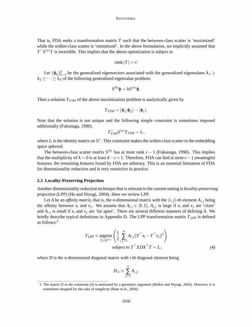
That is, FDA seeks a transformation matrix T such that the between-class scatter is ‘maximized’while the within-class scatter is ‘minimized’. In the above formulation, we implicitly assumed thatT>S(w)T is invertible. This implies that the above optimization is subject to

rank(T ) = r.

Let {ϕk}dk=1 be the generalized eigenvectors associated with the generalized eigenvalues λ1 ≥

λ2 ≥ ·· · ≥ λd of the following generalized eigenvalue problem:

S(b)ϕ = λS(w)ϕ.

Then a solution T FDA of the above maximization problem is analytically given by

T FDA = (ϕ1|ϕ2| · · · |ϕr).

Note that the solution is not unique and the following simple constraint is sometimes imposedadditionally (Fukunaga, 1990).

T>FDAS(w)T FDA = Ir,

where Ir is the identity matrix on Rr. This constraint makes the within-class scatter in the embedding

space sphered.The between-class scatter matrix S(b) has at most rank c− 1 (Fukunaga, 1990). This implies

that the multiplicity of λ = 0 is at least d−c+1. Therefore, FDA can find at most c−1 meaningfulfeatures; the remaining features found by FDA are arbitrary. This is an essential limitation of FDAfor dimensionality reduction and is very restrictive in practice.

2.3 Locality-Preserving Projection

Another dimensionality reduction technique that is relevant to the current setting is locality-preservingprojection (LPP) (He and Niyogi, 2004). Here we review LPP.

Let A be an affinity matrix, that is, the n-dimensional matrix with the (i, j)-th element Ai, j beingthe affinity between xi and x j. We assume that Ai, j ∈ [0,1]; Ai, j is large if xi and x j are ‘close’and Ai, j is small if xi and x j are ‘far apart’. There are several different manners of defining A. Webriefly describe typical definitions in Appendix D. The LPP transformation matrix T LPP is definedas follows:3

T LPP ≡ argminT∈Rd×r

(12

n

∑i, j=1

Ai, j‖T>xi−T>x j‖

2

)

subject to T>XDX>T = Ir, (4)

where D is the n-dimensional diagonal matrix with i-th diagonal element being

Di,i ≡n

∑j=1

Ai, j.

3. The matrix D in the constraint (4) is motivated by a geometric argument (Belkin and Niyogi, 2003). However, it issometimes dropped for the sake of simplicity (Ham et al., 2004).

1030


Eq. (4) implies that LPP looks for a transformation matrix T such that nearby data pairs in theoriginal space R

d are kept close in the embedding space. The constraint (4) is imposed for avoidingdegeneracy.

Let {ψk}dk=1 be the generalized eigenvectors associated with the generalized eigenvalues γ1 ≥

γ2 ≥ ·· · ≥ γd of the following generalized eigenvalue problem:

XLX>ψ = γXDX>ψ,

whereL≡ D−A.

L is called the graph-Laplacian matrix in the spectral graph theory (Chung, 1997), where A is seenas the adjacency matrix of a graph. He and Niyogi (2004) showed that a solution of Eq. (4) is givenby

T LPP = (ψd |ψd−1| · · · |ψd−r+1).

2.4 Typical Behavior of FDA and LPP

Dimensionality reduction results obtained by FDA and LPP are illustrated in Figure 1 (LFDA willbe defined and explained in Section 3)—two-dimensional two-class data samples are embedded intoa one-dimensional space. In LPP, the affinity matrix A is determined by the local scaling method(Zelnik-Manor and Perona, 2005, see also Appendix D.4).

For the simplest data set depicted in Figure 1(a), both FDA and LPP nicely separate the samplesin different classes (‘◦’ and ‘×’) from each other. For the data set depicted in Figure 1(b), FDAstill works well, but LPP mixes samples in different classes into a single cluster. This is caused bythe unsupervised nature of LPP. On the other hand, for the data set depicted in Figure 1(c), LPPworks well but FDA collapses the samples in different classes into a single cluster. The reason forthe failure of FDA is that the ‘levels’ of the between-class scatter and the within-class scatter arenot evaluated in an intuitively natural way because of the two separate clusters in ‘◦’-class (see alsoFukunaga, 1990).

3. Local Fisher Discriminant Analysis

As illustrated in Figure 1, FDA can perform poorly if samples in a class form several separateclusters (i.e., multimodal). In other words, the undesired behavior of FDA is caused by the globalitywhen evaluating the within-class scatter and the between-class scatter (e.g., Figure 1(c)). On theother hand, because of the unsupervised nature of LPP, it can overlap samples in different classes ifthey are close in the original high-dimensional space R

d (e.g., Figure 1(b)).To overcome these problems, we propose combining the ideas of FDA and LPP; more specif-

ically, we evaluate the levels of the between-class scatter and the within-class scatter in a localmanner. This allows us to attain between-class separation and within-class local structure preserva-tion at the same time. We call our new method local Fisher discriminant analysis (LFDA).

3.1 Reformulating FDA

In order to introduce LFDA, let us first reformulate FDA in a pairwise manner.

1031

SUGIYAMA

−10 −5 0 5 10−10

−5

0

5

10

FDALPPLFDA

(a) Toy data set 1

−10 −5 0 5 10−10

−5

0

5

10

FDALPPLFDA

(b) Toy data set 2

−10 −5 0 5 10−10

−5

0

5

10

FDALPPLFDA

(c) Toy data set 3

Figure 1: Examples of dimensionality reduction by FDA, LPP and LFDA. Two-dimensional two-class samples are embedded into a one-dimensional space. The line in the figure denotesthe one-dimensional embedding space (which the data samples are projected on) obtainedby each method.

1032


Lemma 1 S(w) and S(b) defined by Eqs. (1) and (2) can be expressed as

S(w) =12

n

∑i, j=1

W (w)i, j (xi− x j)(xi− x j)

>, (5)

S(b) =12

n

∑i, j=1

W (b)i, j (xi− x j)(xi− x j)

>, (6)

where

W (w)i, j ≡

{1/n` if yi = y j = `,

0 if yi 6= y j,(7)

W (b)i, j ≡

{1/n−1/n` if yi = y j = `,

1/n if yi 6= y j.(8)

A proof of Lemma 1 is given in Appendix A. Note that 1/n−1/n` in Eq. (8) is negative while1/n` and 1/n in Eqs. (7) and (8) are positive. This implies that if the data pairs in the same class aremade close, the within-class scatter matrix S(w) gets ‘small’ and the between-class scatter matrix S(b)

gets ‘large’. On the other hand, if the data pairs in different classes are separated from each other,the between-class scatter matrix S(b) gets ‘large’. Therefore, we may interpret FDA as keeping thesample pairs in the same class close and the sample pairs in different classes apart. A more formaldiscussion on the above interpretation is given in Appendix B.

3.2 Definition and Typical Behavior of LFDA

Based on the above pairwise expression, let us define the local within-class scatter matrix S(w)

and

the local between-class scatter matrix S(b)

as follows.

S(w)≡

12

n

∑i, j=1

W (w)i, j (xi− x j)(xi− x j)

>, (9)

S(b)≡

12

n

∑i, j=1

W (b)i, j (xi− x j)(xi− x j)

>,

where

W (w)i, j ≡

{Ai, j/n` if yi = y j = `,

0 if yi 6= y j,(10)

W (b)i, j ≡

{Ai, j(1/n−1/n`) if yi = y j = `,

1/n if yi 6= y j.(11)

Namely, according to the affinity Ai, j, we weight the values for the sample pairs in the same class.

This means that far apart sample pairs in the same class have less influence on S(w)

and S(b)

. Notethat we do not weight the values for the sample pairs in different classes since we want to separatethem from each other irrespective of the affinity in the original space. From here on, we denote thelocal counterparts of matrices by symbols with tilde.

1033

SUGIYAMA

We define the LFDA transformation matrix T LFDA as

T LFDA ≡ argmaxT∈Rd×r

[tr((T>S

(w)T )−1T>S

(b)T)]

. (12)

That is, we look for a transformation matrix T such that nearby data pairs in the same class aremade close and the data pairs in different classes are separated from each other; far apart data pairsin the same class are not imposed to be close.

Eq. (12) is of the same form as Eq. (3). Therefore, we can similarly compute an analytic form

of T LFDA by solving a generalized eigenvalue problem of S(b)

and S(w)

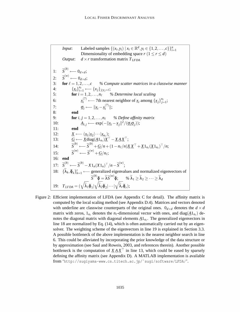
. An efficient implementationof LFDA is summarized as a pseudo code in Figure 2 (see Appendix C for detail).

Toy examples of dimensionality reduction by LFDA are illustrated in Figure 1. We used thelocal scaling method for computing the affinity matrix A (see Appendix D.4). Note that we performthe nearest neighbor search in the local scaling method in a classwise manner since we do notneed the affinity values for the sample pairs in different classes (see Eqs. 10 and 11). This highlycontributes to reducing the computational cost (see Appendix C). Figure 1 shows that LFDA givesdesirable results for all three data sets, that is, LFDA can compensate for the drawbacks of FDA andLPP by effectively combining the ideas of FDA and LPP.

If the affinity value Ai, j is set to 1 for all sample pairs (i.e., all pairs are ‘equally close’ to each

other), S(w)

and S(b)

agree with S(w) and S(b), respectively, and LFDA is reduced to the originalFDA. Therefore, LFDA may be regarded as a natural localized variant of FDA.

3.3 Properties of LFDA

Here we discuss fundamental properties of LFDA.

First, we give an interpretation of LFDA in terms of the ‘pointwise scatter’. S(w)

can be ex-pressed as

S(w)

=12

n

∑i=1

1nyi

P(w)i ,

where nyi is the number of samples in the class to which the sample xi belongs and P(w)i is the

pointwise local within-class scatter matrix around xi:

P(w)i ≡ ∑

j:y j=yi

Ai, j(x j− xi)(x j− xi)>.

Therefore, ‘minimizing’ S(w)

corresponds to minimizing the weighted sum of the pointwise local

within-class scatter matrices over all samples. S(b)

can also be expressed in a similar way as

S(b)

=12

n

∑i=1

(1n−

1nyi

)P

(w)i +

12n

n

∑i=1

P(b)i , (13)

where P(b)i is the pointwise between-class scatter matrix around xi:

P(b)i ≡ ∑

j:y j 6=yi

(x j− xi)(x j− xi)>.

1034


Input: Labeled samples {(xi,yi) | xi ∈ Rd ,yi ∈ {1,2, . . . ,c}}n

i=1Dimensionality of embedding space r (1≤ r ≤ d)

Output: d× r transformation matrix T LFDA

1: S(b)←− 0d×d;

2: S(w)←− 0d×d;

3: for ` = 1,2, . . . ,c % Compute scatter matrices in a classwise manner4: {xi}

n`i=1←− {x j} j:y j=`;

5: for i = 1,2, . . . ,n` % Determine local scaling

6: x(7)i ←− 7th nearest neighbor of xi among {x j}

n`j=1;

7: σi←− ‖xi− x(7)i ‖;

8: end9: for i, j = 1,2, . . . ,n` % Define affinity matrix10: Ai, j←− exp(−‖xi− x j‖

2/(σiσ j));11: end12: X ←− (x1|x2| · · · |xn`

);13: G←− Xdiag(A1n`)X

>−X AX>;

14: S(b)←− S

(b)+G/n+(1−n`/n)X X>+X1n`(X1n`)

>/n;

15: S(w)←− S

(w)+G/n`;

16: end

17: S(b)←− S

(b)−X1n(X1n)

>/n− S(w)

;

18: {λk, ϕk}rk=1←− generalized eigenvalues and normalized eigenvectors of

S(b)

ϕ = λS(w)

ϕ; % λ1 ≥ λ2 ≥ ·· · ≥ λd

19: T LFDA = (

√λ1ϕ1|

√λ2ϕ2| · · · |

√λrϕr);

Figure 2: Efficient implementation of LFDA (see Appendix C for detail). The affinity matrix iscomputed by the local scaling method (see Appendix D.4). Matrices and vectors denotedwith underline are classwise counterparts of the original ones. 0d×d denotes the d× dmatrix with zeros, 1n` denotes the n`-dimensional vector with ones, and diag(A1n`) de-notes the diagonal matrix with diagonal elements A1n` . The generalized eigenvectors inline 18 are normalized by Eq. (14), which is often automatically carried out by an eigen-solver. The weighting scheme of the eigenvectors in line 19 is explained in Section 3.3.A possible bottleneck of the above implementation is the nearest neighbor search in line6. This could be alleviated by incorporating the prior knowledge of the data structure orby approximation (see Saul and Roweis, 2003, and references therein). Another possiblebottleneck is the computation of X A X> in line 13, which could be eased by sparselydefining the affinity matrix (see Appendix D). A MATLAB implementation is availablefrom ‘http://sugiyama-www.cs.titech.ac.jp/˜sugi/software/LFDA/’.

1035

SUGIYAMA

Note that P(b)i does not include the localization factor Ai, j. Eq. (13) implies that ‘maximizing’ S

(b)

corresponds to minimizing the weighted sum of the pointwise local within-class scatter matricesand maximizing the sum of the pointwise between-class scater matrices.

Next, we discuss the issue of eigenvalue multiplicity in LFDA. The original FDA allows us toextract at most c−1 meaningful features since the between-class scatter matrix S(b) has rank at most

c−1 (Fukunaga, 1990). On the other hand, the local between-class scatter matrix S(b)

generally hasa much higher rank with less eigenvalue multiplicity, thanks to the localization factor Ai, j included

in W(b)

(see Eq. 11). In the simulation shown in Section 5, S(b)

is always full rank for various datasets. Therefore, the proposed LFDA can be practically employed for dimensionality reduction intoany dimensional spaces. This is a very important and significant improvement over the originalFDA.

Finally, we discuss the invariance property of LFDA. The value of the LFDA criterion (12) isinvariant under linear transformations, that is, for any r-dimensional invertible matrix H, T LFDAH isalso a solution of Eq. (12). Therefore, the solution T LFDA is not unique—the range of the transfor-mation H>T>LFDA is uniquely determined, but the distance metric (Goldberger et al., 2005; Glober-son and Roweis, 2006; Weinberger et al., 2006) in the embedding space can be arbitrary becauseof the arbitrariness of the matrix H. In practice, we propose determining the LFDA transformationmatrix T LFDA as follows. First, we rescale the generalized eigenvectors {ϕk}

dk=1 so that

ϕkS(w)

ϕk′ =

{1 if k = k′,

0 if k 6= k′.(14)

Note that this rescaling is often automatically carried out by an eigensolver. Then we weight eachgeneralized eigenvector by the square root of its associated generalized eigenvalue, that is,

T LFDA = (

√λ1ϕ1|

√λ2ϕ2| · · · |

√λrϕr), (15)

where λ1 ≥ λ2 ≥ ·· · ≥ λd . This weighting scheme weakens the influence of minor eigenvectors andis shown to work well in experiments (see Section 5).

3.4 Kernel LFDA for Non-Linear Dimensionality Reduction

Here we show how LFDA can be extended to non-linear dimensionality reduction scenarios.As detailed in Appendix C, the generalized eigenvalue problem that needs to be solved in LFDA

can be expressed as

XL(b)

X>ϕ = λXL(w)

X>ϕ, (16)

where L(b)

= L(m)− L

(w)and L

(m)and L

(w)are defined by Eqs. (33) and (35), respectively. Since

X>ϕ in Eq. (16) belongs to the range of X>, it can be expressed by using some vector α ∈ Rn as

X>ϕ = X>Xα = Kα,

where K is the n-dimensional matrix with the (i, j)-th element being

Ki, j ≡ x>i x j.

1036


Then multiplying Eq. (16) by X> from the left-hand side yields

KL(b)

Kα = λKL(w)

Kα. (17)

This implies that {xi}ni=1 appear only in terms of their inner products. Therefore, we can obtain

a non-linear variant of LFDA by the kernel trick (Vapnik, 1998; Scholkopf et al., 1998), which isexplained below.

Let us consider a non-linear mapping φ(x) from Rd to a reproducing kernel Hilbert space H

(Aronszajn, 1950). Let K(x,x′) be the reproducing kernel of H . A typical choice of the kernelfunction would be the Gaussian kernel:

K(x,x′) = exp

(−‖x− x′‖2

2σ2

),

with σ > 0. For other choices, see, for example, Wahba (1990), Vapnik (1998), and Scholkopf andSmola (2002). Because of the reproducing property of K(x,x′), K is now the kernel matrix, that is,the (i, j)-th element is given by

Ki, j = 〈φ(xi),φ(x j)〉= K(xi,x j),

where 〈·, ·〉 denotes the inner product in H .

It can be confirmed that L(w)

is always degenerated (since L(w)

(1,1, . . . ,1)> always vanishes;

see Eq. 35 for detail). Therefore, KL(w)

K is always degenerated and we cannot directly solve the

generalized eigenvalue problem (17). To cope with this problem, we propose regularizing KL(w)

Kand solving the following generalized eigenvalue problem instead (cf. Friedman, 1989).

KL(b)

Kα = λ(KL(w)

K + εIn)α, (18)

where ε is a small constant. Let {αk}nk=1 be the generalized eigenvectors associated with the gener-

alized eigenvalues λ1 ≥ λ2 ≥ ·· · ≥ λn of Eq. (18). Then the embedded image of φ(x′) in H is givenby

(

√λ1α1|

√λ2α2| · · · |

√λrαr)

>

K(x1,x′)K(x2,x′)

...K(xn,x′)

.

We call this kernelized variant of LFDA kernel LFDA (KLFDA).Recently, kernel functions for non-vectorial structured data such as strings, trees, and graphs

have been proposed (see, e.g., Lodhi et al., 2002; Duffy and Collins, 2002; Kashima and Koyanagi,2002; Kondor and Lafferty, 2002; Kashima et al., 2003; Gartner et al., 2003; Gartner, 2003). SinceKLFDA uses the samples only via the kernel function K(x,x′), it allows us to reduce the dimension-ality of such non-vectorial data.

4. Comparison with Related Methods

In this section, we discuss the relation between the proposed LFDA and other methods.

1037

SUGIYAMA

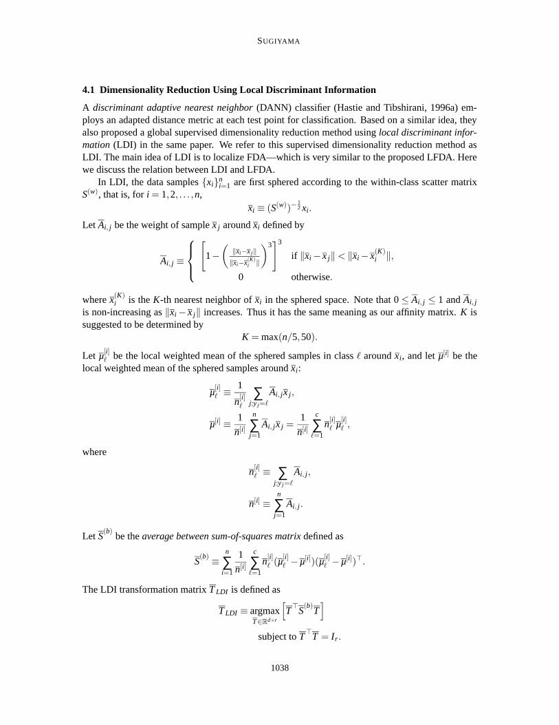
4.1 Dimensionality Reduction Using Local Discriminant Information

A discriminant adaptive nearest neighbor (DANN) classifier (Hastie and Tibshirani, 1996a) em-ploys an adapted distance metric at each test point for classification. Based on a similar idea, theyalso proposed a global supervised dimensionality reduction method using local discriminant infor-mation (LDI) in the same paper. We refer to this supervised dimensionality reduction method asLDI. The main idea of LDI is to localize FDA—which is very similar to the proposed LFDA. Herewe discuss the relation between LDI and LFDA.

In LDI, the data samples {xi}ni=1 are first sphered according to the within-class scatter matrix

S(w), that is, for i = 1,2, . . . ,n,xi ≡ (S(w))−

12 xi.

Let Ai, j be the weight of sample x j around xi defined by

Ai, j ≡

[1−

(‖xi−x j‖

‖xi−x(K)i ‖

)3]3

if ‖xi− x j‖< ‖xi− x(K)i ‖,

0 otherwise.

where x(K)i is the K-th nearest neighbor of xi in the sphered space. Note that 0 ≤ Ai, j ≤ 1 and Ai, j

is non-increasing as ‖xi− x j‖ increases. Thus it has the same meaning as our affinity matrix. K issuggested to be determined by

K = max(n/5,50).

Let µ[i]` be the local weighted mean of the sphered samples in class ` around xi, and let µ[i] be the

local weighted mean of the sphered samples around xi:

µ[i]` ≡

1

n[i]`

∑j:y j=`

Ai, jx j,

µ[i] ≡1

n[i]

n

∑j=1

Ai, jx j =1

n[i]

c

∑=1

n[i]` µ[i]

` ,

where

n[i]` ≡ ∑

j:y j=`

Ai, j,

n[i] ≡n

∑j=1

Ai, j.

Let S(b)

be the average between sum-of-squares matrix defined as

S(b)≡

n

∑i=1

1

n[i]

c

∑=1

n[i]` (µ[i]

` −µ[i])(µ[i]` −µ[i])>.

The LDI transformation matrix T LDI is defined as

T LDI ≡ argmaxT∈Rd×r

[T>

S(b)

T]

subject to T>

T = Ir.

1038


T LDI is a transformation matrix for sphered samples; the LDI transformation matrix T LDI for non-sphered samples is given by

T LDI = (S(w))−12 T LDI .

Similar to FDA (and LFDA), T LDI can be efficiently computed by solving a generalized eigenvalueproblem.

The average between sum-of-squares matrix S(b)

is conceptually very similar to the local between-

class scatter matrix S(b)

in LFDA. Indeed, as proved in Appendix E, we can express S(b)

in a pairwisemanner as

S(b)

=12

n

∑i, j=1

W(b)i, j (xi− x j)(xi− x j)

>, (19)

where

W(b)i, j ≡

n

∑k=1

1

n[k]

(1

n[k]−

1

n[k]`

)Ai,kA j,k if yi = y j = `,

n

∑k=1

1

(n[k])2Ai,kA j,k if yi 6= y j.

(20)

However, there exist critical differences between LDI and LFDA. A significant difference is that thevalues for the sample pairs in different classes are also localized in LDI (see Eq. 20), while they arekept unlocalized in LFDA (see Eq. 11). This implies that far apart sample pairs in different classescould be made close in LDI, which is not desirable in supervised dimensionality reduction. Further-

more, the computation of S(b)

is slightly less efficient than S(b)

since W(b)

includes the summationover k.

Another important difference between LDI and LFDA is that the within-class scatter matrix S(w)

is not localized in LDI. However, as we showed in Section 3.1, the within-class scatter matrix S(w)

also accounts for collapsing the within-class multimodal structure (i.e., far apart sample pairs in thesame class are made close). This phenomenon is experimentally confirmed in Section 5.2.

4.2 Mixture Discriminant Analysis

FDA can be interpreted as maximum likelihood estimation of Gaussian distributions with commoncovariance and different means for each class. Based on this view, Hastie and Tibshirani (1996b)proposed mixture discriminant analysis (MDA), which extends FDA to maximum likelihood esti-mation of Gaussian mixture distributions.

A maximum likelihood solution is obtained by an EM-type algorithm (cf. Dempster et al., 1977).However, this is an iterative algorithm and gives only a local optimal solution. Therefore, the com-putation of MDA is rather slow and there is no guarantee that the global solution can be obtained.Furthermore, the number of mixture components (clusters) in each class as well as the initial loca-tion of cluster centers should be determined by users. For cluster centers, using standard techniquessuch as k-means clustering (MacQueen, 1967; Everitt et al., 2001) or learning vector quantization(Kohonen, 1989) are recommended. However, they are also iterative algorithms and have no guar-antee that the global solution can be obtained. Furthermore, there seems to be no systematic methodfor determining the number of clusters.

On the other hand, the proposed LFDA contains no tuning parameters (given that the affinitymatrix is determined by the local scaling method, see Appendix D.4) and the global solution can

1039

SUGIYAMA

be obtained analytically. However, it still lacks a probabilistic interpretation, which remains opencurrently.

4.3 Neighborhood Component Analysis

Goldberger et al. (2005) proposed a supervised dimensionality reduction method called neighbor-hood component analysis (NCA). The NCA transformation matrix T NCA is defined as follows.

T NCA ≡ argmaxT∈Rd×r

(n

∑i=1

∑j:y j=yi

pi, j(T T>)

), (21)

where

pi, j(U)≡

exp{−(xi− x j)

>U(xi− x j)}

∑k 6=i exp{−(xi− xk)>U(xi− xk)}if i 6= j,

0 if i = j.

(22)

The above definition corresponds to maximizing the expected number of correctly classified samplesby a stochastic variant of nearest neighbor classifiers. Therefore, NCA seeks a transformation matrixT such that the between-class separability is maximized.

Eqs. (21) and (22) imply that nearby data pairs in the same class are made close, which issimilar to the proposed LFDA. Indeed, the simulation results in Section 5.2 show that NCA tendsto preserve the multimodal structure of the data very well. However, a crucial weakness of NCAis optimization: the optimization problem (21) is non-convex. Therefore, there is no guarantee thatthe globally optimal solution can be obtained. Goldberger et al. (2005) proposed using a gradientascent method for optimization:

T ← T + ε∇JNCA(T ), (23)

where ε (> 0) is the step size and the gradient ∇JNCA(T ) is given by

∇JNCA(T ) = 2Tn

∑i=1

({

∑j:y j=yi

pi, j(T T>)

}{n

∑j=1

pi, j(T T>)(xi− x j)(xi− x j)>

}

− ∑j:y j=yi

pi, j(T T>)(xi− x j)(xi− x j)>

).

The gradient ascent iteration (23) is computationally rather inefficient. Also, the choice of the stepsize ε is troublesome. If the step size is small enough, the convergence to one of the local optimais guaranteed but such a choice makes the convergence very slow; on the other hand, if the stepsize is too large, gradient flows oscillate and proper convergence properties may not be guaranteedanymore. Furthermore, the choice of the termination condition in the iterative algorithm is oftencumbersome in practice.

Because of the non-convexity of the optimization problem, the quality of the obtained solutiondepends on the initialization of the matrix T . A useful heuristic to alleviate the local optimumproblem is to employ the FDA (or LFDA) result as an initial matrix for optimization (Goldbergeret al., 2005). In the experiments in Section 5, using the LFDA result as an initial matrix appears tobe better than the random initialization. However, the local optima problem still remains even withthe above heuristic.

1040


When a dimensionality reduction technique is applied to classification tasks, we often want toembed the data samples into spaces with several different dimensions—the best dimensionality islater chosen by, for example, cross-validation (Stone, 1974; Wahba, 1990). In such a scenario,NCA requires to optimize the transformation matrix individually for each dimensionality r of theembedding space. On the other hand, LFDA needs to compute the transformation matrix only oncefor the largest r; its sub-matrices become the optimal solutions for smaller dimensions. Therefore,LFDA is computationally more efficient than NCA in this scenario.

A simple MATLAB implementation of NCA is available.4 We use this software in Section 5.

4.4 Maximally Collapsing Metric Learning

In order to overcome the computational problem of NCA, Globerson and Roweis (2006) proposedan alternative method called maximally collapsing metric learning (MCML).

Let p∗i, j be the ‘ideal’ value of pi, j(U) defined by Eq. (22):

p∗i, j ∝

{1 if yi = y j,

0 if yi 6= y j,

where p∗i, j is normalized so that

∑j 6=i

p∗i, j = 1.

p∗i, j can be attained if all samples in the same class collapse into a single point while samplesin other classes are mapped to other locations. In reality, however, any U may not be able toattain pi, j(U) = p∗i, j exactly; instead the optimal approximation to p∗i, j under the Kullback-Leiblerdivergence (Kullback and Leibler, 1951) is obtained. This is formally defined as

UMCML ≡ argminU∈Rd×d

(n

∑i, j=1

p∗i, j logp∗i, j

pi, j(U)

)

subject to U ∈ PSD(r), (24)

where PSD(r) is the set of all positive semidefinite matrices of rank r (i.e., r eigenvalues are pos-itive and others are zero). Once U MCML is obtained, the MCML transformation matrix T MCML iscomputed by

T MCML = (φ1|φ2| · · · |φr), (25)

where {φk}rk=1 are the eigenvectors associated with the positive eigenvalues η1 ≥ η2 ≥ ·· · ≥ ηr > 0

of the following eigenvalue problem:

UMCMLφ = ηφ.

One of the motivations of MCML is to alleviate the difficulty of optimization in NCA. However,MCML still has a weakness in optimization: the optimization problem (24) is convex only whenr = d, that is, the dimensionality is not reduced but only the distance metric of the original space ischanged. This means that if r < d (which is our primal focus in this paper), we may not be able to

4. Implementation available at ‘http://www.cs.berkeley.edu/˜fowlkes/software/nca/’.

1041

SUGIYAMA

obtain the globally optimal solution. Globerson and Roweis (2006) proposed the following heuristicalgorithm to approximate T MCML.

First, the optimization problem (24) with r = d is solved:

UMCML ≡ argminU∈Rd×d

(n

∑i, j=1

p∗i, j logp∗i, j

pi, j(U)

)

subject to U ∈ PSD(d). (26)

Although Eq. (26) is convex, an analytic form of the unique optimal solution UMCML is not knownyet. Globerson and Roweis (2006) proposed using the following alternate iterative procedure forobtaining UMCML.

U ←U− ε∇JMCML(U), (27)

U ←d

∑k=1

max(0, ηk)φkφ>

k , (28)

where ε (> 0) is the step size, ηk and φk are eigenvalues and eigenvectors of U , and the gradient∇JMCML(U) is given by

∇JMCML(U) =n

∑i, j=1

(p∗i, j− pi, j(U))(xi− x j)(xi− x j)>.

Then the eigenvalue decomposition of UMCML is carried out and eigenvalues η1 ≥ η2 ≥ ·· · ≥ ηd

and associated eigenvectors {φk}dk=1 are obtained:

UMCMLφ = ηφ.

Finally, {φk}rk=1 in Eq. (25) are replaced by {φk}

rk=1, which yields

T MCML ≈ (φ1|φ2| · · · |φr). (29)

This approximation is shown to be practically useful (Globerson and Roweis, 2006), although thereseems to be no theoretical analysis for this approximation.

MCML may have an advantage over NCA in computation: there exists the analytic approx-imation (29) that can be computed efficiently using the solution of another convex optimizationproblem (26). However, MCML still relies on the gradient-based alternate iterative algorithm (27)–(28) to solve the convex optimization problem (26), which is computationally very expensive sincethe eigenvalue decomposition of a d-dimensional matrix should be carried out in each iteration (seeEq. 28). Furthermore, the difficulty of appropriately choosing the step size and the terminationcondition in the iterative procedure still remains.

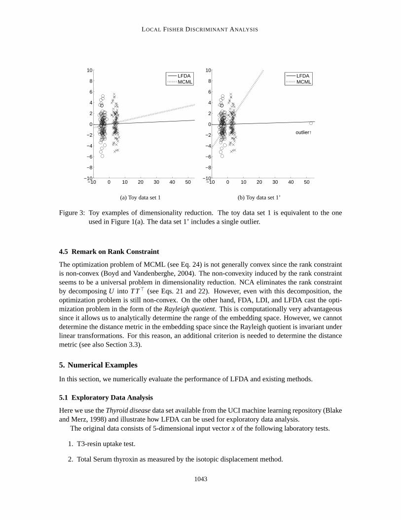
Since MCML requires all the samples in the same class to collapse into a single point, it isnot necessarily useful in dimensionality reduction of multimodal data samples. Furthermore, theMCML results can be significantly influenced by outliers since the outliers are also required tocollapse into the same single point together with other samples. This phenomenon is illustrated inFigure 3, where a single outlier significantly changes the MCML result.

Globerson and Roweis (2006) showed that the sufficient statistics of the MCML algorithm arepointwise scatter matrices (cf. Section 3.3). Since LFDA also has an interpretation in terms ofpointwise scatter matrices, there may be a link between LFDA and MCML and this needs to beinvestigated in the future work.

1042


−10 0 10 20 30 40 50−10

−8

−6

−4

−2

0

2

4

6

8

10LFDAMCML

(a) Toy data set 1

−10 0 10 20 30 40 50−10

−8

−6

−4

−2

0

2

4

6

8

10

outlier↑

LFDAMCML

(b) Toy data set 1’

Figure 3: Toy examples of dimensionality reduction. The toy data set 1 is equivalent to the oneused in Figure 1(a). The data set 1’ includes a single outlier.

4.5 Remark on Rank Constraint

The optimization problem of MCML (see Eq. 24) is not generally convex since the rank constraintis non-convex (Boyd and Vandenberghe, 2004). The non-convexity induced by the rank constraintseems to be a universal problem in dimensionality reduction. NCA eliminates the rank constraintby decomposing U into T T> (see Eqs. 21 and 22). However, even with this decomposition, theoptimization problem is still non-convex. On the other hand, FDA, LDI, and LFDA cast the opti-mization problem in the form of the Rayleigh quotient. This is computationally very advantageoussince it allows us to analytically determine the range of the embedding space. However, we cannotdetermine the distance metric in the embedding space since the Rayleigh quotient is invariant underlinear transformations. For this reason, an additional criterion is needed to determine the distancemetric (see also Section 3.3).

5. Numerical Examples

In this section, we numerically evaluate the performance of LFDA and existing methods.

5.1 Exploratory Data Analysis

Here we use the Thyroid disease data set available from the UCI machine learning repository (Blakeand Merz, 1998) and illustrate how LFDA can be used for exploratory data analysis.

The original data consists of 5-dimensional input vector x of the following laboratory tests.

1. T3-resin uptake test.

2. Total Serum thyroxin as measured by the isotopic displacement method.

1043

SUGIYAMA

−25 −20 −15 −10 −50

2

4

6

8

First Feature

HyperthyroidismHypothyroidism

−25 −20 −15 −10 −50

5

10

15

20

25

30

First Feature

Euthyroidism

(a) FDA

3 4 5 6 70

2

4

6

8

First Feature

HyperthyroidismHypothyroidism

3 4 5 6 70

5

10

15

20

First Feature

Euthyroidism

(b) LFDA

Figure 4: Histograms of the first feature values obtained by FDA and LFDA for the Thyroid diseasedata set. The top row corresponds to the sick patients and the bottom row corresponds tothe healthy patients.

3. Total Serum triiodothyronine as measured by radioimmuno assay.

4. Basal thyroid-stimulating hormone (TSH) as measured by radioimmuno assay.

5. Maximal absolute difference of TSH value after injection of 200 micro grams of thyrotropin-releasing hormone as compared to the basal value.

The task is to predict whether patients’ thyroids are euthyroidism, hypothyroidism, or hyperthy-roidism (Coomans et al., 1983), that is, whether patients’ thyroids are normal, hypo-functioning,or hyper-functioning (Blake and Merz, 1998). The diagnosis (the class label) is based on a com-plete medical record, including anamnesis, scan etc. Here we merge the hypothyroidism class andthe hyperthyroidism class into a single class and create binary labeled data (whether thyroids arenormal or not). Our goal is to predict whether patients’ thyroids are normal, hypo-functioning, orhyper-functioning from the binary labeled data samples.

Figure 4 depicts the histograms of the first feature values obtained by FDA and LFDA—thetop row corresponds to the sick patients and the bottom row corresponds to the healthy patients.This shows that both FDA and LFDA separate the patients with normal thyroids from sick patientsreasonably well. In addition to between-class separability, LFDA clearly preserves the multimodalstructure among sick patients (i.e., hypo-functioning and hyper-functioning), which is lost by or-dinary FDA. Another interesting finding from the figure is that the first feature values obtained byLFDA has a strong negative correlation to the functioning level of thyroids—this could be used forpredicting the functioning level of thyroids.

1044


Data Set d ‘◦’-and-‘•’ class ‘×’ classLetter recognition 16 ‘A’ & ‘C’ ‘B’

Iris 4 ‘Setosa’ & ‘Virginica’ ‘Versicolour’

Table 1: Two-class data sets used for visualization experiments (r = 2).

5.2 Data Visualization

Here we apply the proposed and existing dimensionality reduction methods to benchmark data setsand investigate how they behave in data visualization tasks.

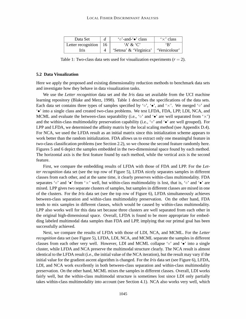
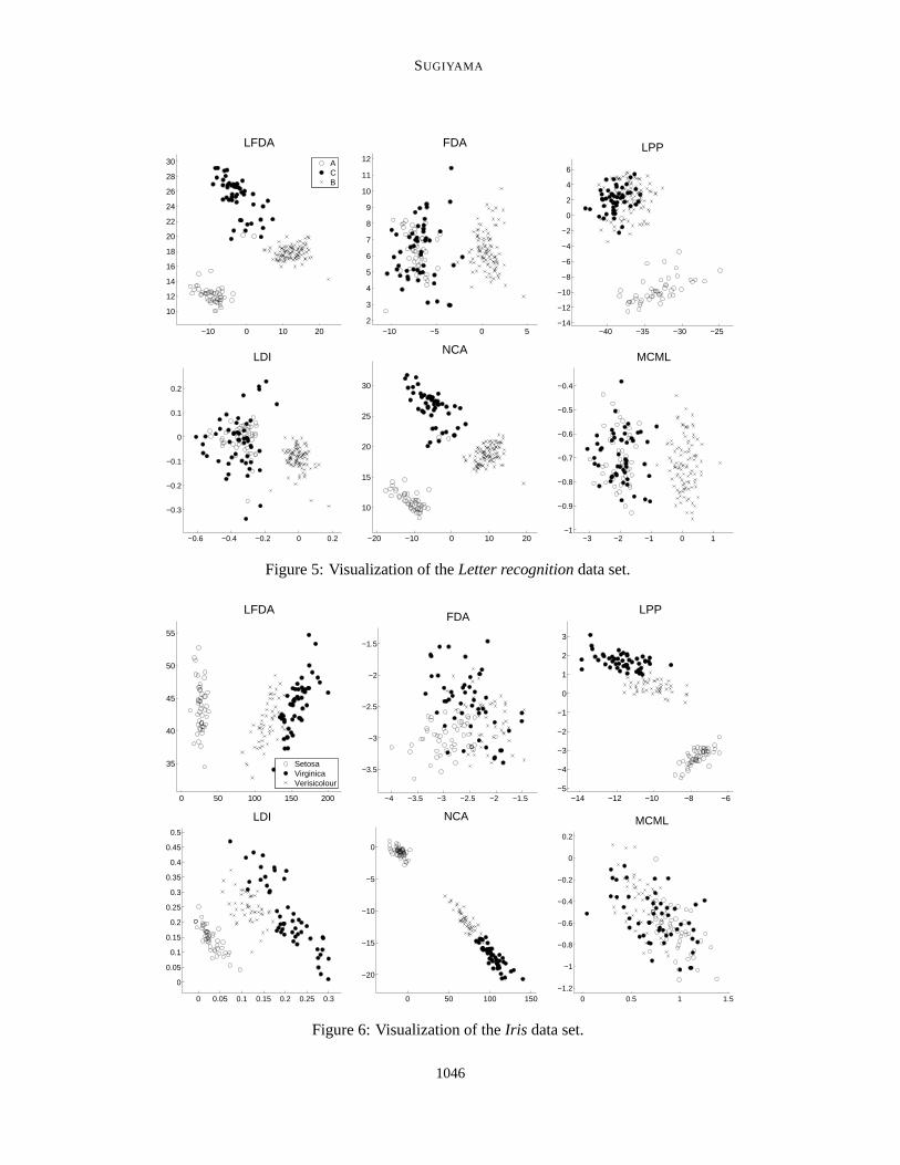
We use the Letter recognition data set and the Iris data set available from the UCI machinelearning repository (Blake and Merz, 1998). Table 1 describes the specifications of the data sets.Each data set contains three types of samples specified by ‘◦’, ‘•’, and ‘×’. We merged ‘◦’ and‘•’ into a single class and created two-class problems. We test LFDA, FDA, LPP, LDI, NCA, andMCML and evaluate the between-class separability (i.e., ‘◦’ and ‘•’ are well separated from ‘×’)and the within-class multimodality preservation capability (i.e., ‘◦’ and ‘•’ are well grouped). ForLPP and LFDA, we determined the affinity matrix by the local scaling method (see Appendix D.4).For NCA, we used the LFDA result as an initial matrix since this initialization scheme appears towork better than the random initialization. FDA allows us to extract only one meaningful feature intwo-class classification problems (see Section 2.2), so we choose the second feature randomly here.Figures 5 and 6 depict the samples embedded in the two-dimensional space found by each method.The horizontal axis is the first feature found by each method, while the vertical axis is the secondfeature.

First, we compare the embedding results of LFDA with those of FDA and LPP. For the Let-ter recognition data set (see the top row of Figure 5), LFDA nicely separates samples in differentclasses from each other, and at the same time, it clearly preserves within-class multimodality. FDAseparates ‘◦’ and ‘•’ from ‘×’ well, but within-class multimodality is lost, that is, ‘◦’ and ‘•’ aremixed. LPP gives two separate clusters of samples, but samples in different classes are mixed in oneof the clusters. For the Iris data set (see the top row of Figure 6), LFDA simultaneously achievesbetween-class separation and within-class multimodality preservation. On the other hand, FDAtends to mix samples in different classes, which would be caused by within-class multimodality.LPP also works well for this data set because three clusters are well separated from each other inthe original high-dimensional space. Overall, LFDA is found to be more appropriate for embed-ding labeled multimodal data samples than FDA and LPP, implying that our primal goal has beensuccessfully achieved.

Next, we compare the results of LFDA with those of LDI, NCA, and MCML. For the Letterrecognition data set (see Figure 5), LFDA, LDI, NCA, and MCML separate the samples in differentclasses from each other very well. However, LDI and MCML collapse ‘◦’ and ‘•’ into a singlecluster, while LFDA and NCA preserve the multimodal structure clearly. The NCA result is almostidentical to the LFDA result (i.e., the initial value of the NCA iteration), but the result may vary if theinitial value for the gradient ascent algorithm is changed. For the Iris data set (see Figure 6), LFDA,LDI, and NCA work excellently in both between-class separation and within-class multimodalitypreservation. On the other hand, MCML mixes the samples in different classes. Overall, LDI worksfairly well, but the within-class multimodal structure is sometimes lost since LDI only partiallytakes within-class multimodality into account (see Section 4.1). NCA also works very well, which

1045

SUGIYAMA

−10 0 10 20

10

12

14

16

18

20

22

24

26

28

30

LFDA

ACB

−10 −5 0 52

3

4

5

6

7

8

9

10

11

12

FDA

−40 −35 −30 −25−14

−12

−10

−8

−6

−4

−2

0

2

4

6

LPP

−0.6 −0.4 −0.2 0 0.2

−0.3

−0.2

−0.1

0

0.1

0.2

LDI

−20 −10 0 10 20

10

15

20

25

30

NCA

−3 −2 −1 0 1−1

−0.9

−0.8

−0.7

−0.6

−0.5

−0.4

MCML

Figure 5: Visualization of the Letter recognition data set.

0 50 100 150 200

35

40

45

50

55

LFDA

SetosaVirginicaVerisicolour

−4 −3.5 −3 −2.5 −2 −1.5

−3.5

−3

−2.5

−2

−1.5

FDA

−14 −12 −10 −8 −6−5

−4

−3

−2

−1

0

1

2

3

LPP

0 0.05 0.1 0.15 0.2 0.25 0.3

0

0.05

0.1

0.15

0.2

0.25

0.3

0.35

0.4

0.45

0.5

LDI

0 50 100 150

−20

−15

−10

−5

0

NCA

0 0.5 1 1.5−1.2

−1

−0.8

−0.6

−0.4

−0.2

0

0.2

MCML

Figure 6: Visualization of the Iris data set.

1046


Data nameInput

dimensionality

# oftrainingsamples

# oftest

samples

# ofrealizations

∗banana 2 400 4900 100breast-cancer 9 200 77 100

diabetes 8 468 300 100flare-solar 9 666 400 100

german 20 700 300 100heart 13 170 100 100image 18 1300 1010 20

ringnorm 20 400 7000 100splice 60 1000 2175 20∗thyroid 5 140 75 100titanic 3 150 2051 100

twonorm 20 400 7000 100∗waveform 21 400 4600 100∗USPS-eo 256 1000 1000 20∗USPS-sl 256 1000 1000 20

Table 2: List of binary classification data sets. Data sets indicated by ‘∗’ contain intrinsic within-class multimodal structures.

implies that the heuristic to use the LFDA result as an initial value is useful. However, NCA doesnot provide significant performance improvement over LFDA in the above simulations. The MCMLresults have similar tendencies to FDA.

Based on the above simulation results, we conclude that LFDA is a promising method in thevisualization of multimodal labeled data.

5.3 Classification

Here we apply the proposed and existing dimensionality reduction techniques to classification tasks,and objectively evaluate the effectiveness of LFDA.

There are several measures for quantitatively evaluating separability of data samples in differentclasses (e.g., Fukunaga, 1990; Globerson et al., 2005). Here we use a simple one: misclassifica-tion rate by a one-nearest-neighbor classifier. As explained in Section 3.3, the LFDA criterionis invariant under linear transformations, while the misclassification rate by a one-nearest-neighborclassifier depends on the distance metric. This means that the following simulation results are highlydependent on the normalization scheme (15).

We employ the IDA data sets,5 which are standard binary classification data sets originally usedin Ratsch et al. (2001). In addition, we use two binary classification data sets created from the USPShandwritten digit data set. The first task (USPS-eo) is to separate even numbers from odd numbersand the second task (USPS-sl) is to separate small numbers (‘0’ to ‘4’) from large numbers (‘5’ to‘9’). For training and testing, 100 samples are randomly chosen for each digit. Table 2 summarizes

5. Data sets available at http://ida.first.fraunhofer.de/projects/bench/benchmarks.htm.

1047

SUGIYAMA

Data set LFDA LDI NCA MCML LPP PCA∗banana ◦13.7±0.8 ◦13.6±0.8 14.3±2.0 39.4±6.7 ◦13.6±0.8 ◦13.6±0.8

breast-cancer ◦34.7±4.3 36.4±4.9 34.9±5.0 ◦34.0±5.8 ◦33.5±5.4 ◦34.5±5.0diabetes 32.0±2.5 ◦30.8±1.9 — ◦31.2±2.1 31.5±2.5 ◦31.2±3.0

flare-solar ◦39.2±5.0 ◦39.3±4.8 — — ◦39.2±4.9 ◦39.1±5.1german ◦29.9±2.8 30.7±2.4 ◦29.8±2.6 31.3±2.4 30.7±2.4 ◦30.2±2.4heart ◦21.9±3.7 23.9±3.1 23.0±4.3 23.3±3.8 23.3±3.8 24.3±3.5image ◦3.2±0.8 ◦3.0±0.6 — 4.7±0.8 3.6±0.7 ◦3.4±0.5

ringnorm 21.1±1.3 ◦17.5±1.0 21.8±1.3 22.0±1.2 20.6±1.1 21.6±1.4splice ◦16.9±0.9 17.9±0.8 — ◦17.3±0.9 23.2±1.2 22.6±1.3∗thyroid ◦4.6±2.6 8.0±2.9 ◦4.5±2.2 18.5±3.8 ◦4.2±2.9 ◦4.9±2.6titanic ◦33.1±11.9 ◦33.1±11.9 ◦33.0±11.9 ◦33.1±11.9 ◦33.0±11.9 ◦33.0±12.0

twonorm ◦3.5±0.4 4.1±0.6 3.7±0.6 ◦3.5±0.4 3.7±0.7 3.6±0.6∗waveform ◦12.5±1.0 20.7±2.5 ◦12.6±0.8 17.9±1.5 ◦12.4±1.0 12.7±1.2∗USPS1 9.0±0.8 12.5±0.9 — — 7.2±1.0 ◦3.5±0.7∗USPS2 12.9±1.2 25.9±1.7 — 11.7±1.3 7.5±0.8 ◦3.9±0.8

Computationtime (ratio)

1.00 1.11 97.23 70.61 1.04 0.91

Table 3: Means and standard deviations of the misclassification rate when the embedding dimen-sionality is chosen by cross validation. For each data set, the best method and comparableones based on the t-test at the significance level 5% are marked by ‘◦’. Data sets indicatedby ‘∗’ contain the intrinsic within-class multimodal structure.

the specifications of the data sets. The ringnorm, twonorm, and waveform data sets contain featureswith only noise. The thyroid, waveform, USPS-eo, and USPS-sl data sets contain intrinsic within-class multimodal structures since they are converted from multi-class problems by merging some ofthe classes. The banana data set is also multimodal.

We test LFDA, LDI, NCA, MCML, LPP, and principal component analysis (PCA). Note thatLPP and PCA are unsupervised dimensionality reduction methods, while others are supervisedmethods. NCA is not tested for the diabetes, flare-solar, image, splice, USPS-eo, and USPS-sldata sets and MCML is not tested for the flare-solar and USPS-eo data sets since the execution timeis too long.

Figure 7 depicts the mean misclassification rate by a one-nearest-neighbor classifier as functionsof the dimensionality r of the reduced space. The error bars are omitted for clear visibility. Instead,we plotted the results of the following significance test: for each dimensionality r, the mean mis-classification rate by the best method and comparable ones based on the t-test (Henkel, 1979) at thesignificance level 5% are marked by ‘◦’. The results show that LFDA works quite well, but overallthere is no single best method that consistently outperforms the others.

Table 3 describes the mean and standard deviation of the misclassification rate by each methodwhen the embedding dimensionality r is chosen by 5-fold cross validation (Stone, 1974; Wahba,1990); for the USPS-eo and USPS-sl data sets, we used 20-fold cross validation since this wasmore accurate. For each data set, the best method and comparable ones based on the t-test atthe significance level 5% are indicated by ‘◦’. The table shows that overall LFDA has excellent

1048


1 2

0.15

0.2

0.25

0.3

0.35

0.4M

ean

Mis

clas

sific

atio

n R

ate

Reduced Dimension r

banana

LFDALDINCAMCMLLPPPCA

1 2 3 4 5 6 7 8 9

0.32

0.33

0.34

0.35

0.36

0.37

0.38

Mea

n M

iscl

assi

ficat

ion

Rat

e

Reduced Dimension r

breast−cancer

1 2 3 4 5 6 7 80.3

0.31

0.32

0.33

0.34

0.35

0.36

0.37

0.38

Mea

n M

iscl

assi

ficat

ion

Rat

e

Reduced Dimension r

diabetes

1 2 3 4 5 6 7 8 9

0.39

0.391

0.392

0.393

0.394

0.395

Mea

n M

iscl

assi

ficat

ion

Rat

e

Reduced Dimension r

flare−solar

5 10 15 20

0.3

0.32

0.34

0.36

0.38

0.4

0.42

Mea

n M

iscl

assi

ficat

ion

Rat

e

Reduced Dimension r

german

2 4 6 8 10 12

0.21

0.22

0.23

0.24

0.25

0.26

0.27

Mea

n M

iscl

assi

ficat

ion

Rat

e

Reduced Dimension r

heart

2 4 6 8 10 12 14 16 18

0.05

0.1

0.15

0.2

0.25

0.3

0.35

Mea

n M

iscl

assi

ficat

ion

Rat

e

Reduced Dimension r

image

5 10 15 20

0.18

0.2

0.22

0.24

0.26

0.28

0.3

0.32

0.34

0.36

Mea

n M

iscl

assi

ficat

ion

Rat

e

Reduced Dimension r

ringnorm

0 10 20 30 40 50 60

0.2

0.25

0.3

0.35

0.4

0.45

Mea

n M

iscl

assi

ficat

ion

Rat

e

Reduced Dimension r

splice

1 2 3 4 5

0.04

0.06

0.08

0.1

0.12

0.14

0.16

0.18

0.2

Mea

n M

iscl

assi

ficat

ion

Rat

e

Reduced Dimension r

thyroid

1 2 3

0.33

0.335

0.34

0.345

Mea

n M

iscl

assi

ficat

ion

Rat

e

Reduced Dimension r

titanic

5 10 15 20

0.035

0.04

0.045

0.05

0.055

0.06

0.065

Mea

n M

iscl

assi

ficat

ion

Rat

e

Reduced Dimension r

twonorm

0 5 10 15 20

0.12

0.14

0.16

0.18

0.2

0.22

0.24

0.26

Mea

n M

iscl

assi

ficat

ion

Rat

e

Reduced Dimension r

waveform

0 50 100 150 200 250

0.05

0.1

0.15

0.2

0.25

0.3

0.35

0.4

0.45

0.5

Mea

n M

iscl

assi

ficat

ion

Rat

e

Reduced Dimension r

USPS−eo

0 50 100 150 200 250

0.05

0.1

0.15

0.2

0.25

0.3

0.35

0.4

0.45

0.5

Mea

n M

iscl

assi

ficat

ion

Rat

e

Reduced Dimension r

USPS−sl

Figure 7: Mean misclassification rates by a one-nearest-neighbor method as functions of the dimen-sionality of the embedding space. For each dimension, the best method and comparableones based on the t-test at the significance level 5% are marked by ‘◦’.

1049

SUGIYAMA

Data set LFDA EUCLID FDA∗banana ◦13.7±0.8 ◦13.6±0.8 ◦13.6±0.8

breast-cancer 34.7±4.3 ◦32.7±4.8 ◦32.9±4.5diabetes 32.0±2.5 ◦30.1±2.1 ◦30.6±2.2

flare-solar ◦39.2±5.0 ◦39.2±5.1 ◦39.0±4.9german ◦29.9±2.8 ◦29.5±2.5 30.5±2.8heart ◦21.9±3.7 23.2±3.7 24.0±3.7image ◦3.2±0.8 ◦3.4±0.5 6.5±1.7

ringnorm ◦21.1±1.3 35.0±1.4 31.2±1.6splice ◦16.9±0.9 28.9±1.5 33.7±1.5∗thyroid ◦4.6±2.6 ◦4.4±2.2 5.3±2.5titanic ◦33.1±11.9 ◦33.0±11.9 ◦33.1±11.9

twonorm ◦3.5±0.4 6.7±0.7 5.0±0.7∗waveform ◦12.5±1.0 15.8±0.7 17.6±1.4∗USPS-eo 9.0±0.8 ◦3.6±0.7 15.1±2.4∗USPS-sl 12.9±1.2 ◦3.8±0.8 13.3±2.9

Table 4: Means and standard deviations of the misclassification rate. The LFDA results are copiedfrom Table 3. ‘EUCLID’ denotes a naive one-nearest-neighbor classification without di-mensionality reduction. ‘FDA’ denotes a naive one-nearest-neighbor classification afterthe samples are projected onto a one-dimensional FDA subspace.

performance. LDI and MCML also work quite well, but they tend to perform rather poorly for themultimodal data sets specified by ‘∗’. NCA also works well, but it does not compare favorably withLFDA. Note that NCA with random initialization was slightly worse; therefore our heuristic to usethe LFDA results for initialization would be reasonable. LPP and PCA perform well, despite thefact that they are unsupervised dimensionality reduction methods. In particular, PCA has excellentperformance for the USPS data sets since the projection onto the two-dimensional PCA subspacealready gives reasonably separate embedding (He and Niyogi, 2004).

The computation time of each method summed over 9 data sets for which NCA is tested isdescribed in the bottom of Table 3. For better comparison, we normalized the values by the com-putation time of LFDA. This shows that LFDA is much faster than NCA and MCML,6 and iscomparable to LDI, LPP, and PCA.

The misclassification rates by a naive one-nearest-neighbor classification without dimensional-ity reduction (‘EUCLID’) are described in Table 4. The table shows that, on the whole, the per-formance of LFDA is comparable to EUCLID. This implies that the use of LFDA is advantageouswhen the dimensionality of the original data is very high since the computation time in the test phasecan be reduced. Table 4 also includes the misclassification rates by a naive one-nearest-neighborclassification after the samples are projected onto a one-dimensional FDA subspace, showing thatLFDA tends to outperform FDA.

6. In our implementation of MCML, we used a constant step size for the gradient descent. The computation time couldbe improved if, for example, an Armijo like step size rule (Bertsekas, 1976) is employed.

1050


Based on the above simulation results, we conclude that the proposed LFDA is a promisingdimensionality reduction technique also in classification scenarios.

6. Conclusions

We discussed the problem of supervised dimensionality reduction. FDA (Fisher, 1936; Fukunaga,1990; Duda et al., 2001) works well for this purpose, given that data samples in each class are uni-modal Gaussian. However, samples in a class are often multimodal in practice, for example, whenmulti-class classification problems are solved by a set of two-class ‘one-versus-rest’ problems. LPP(He and Niyogi, 2004) can work well in dimensionality reduction of multimodal data. However, itis an unsupervised method and does not necessarily useful in supervised dimensionality reductionscenarios. In this paper, we proposed a new method called LFDA, which effectively combines theideas of FDA and LPP. LFDA allows us to reduce the dimensionality of multimodal labeled dataappropriately by maximizing between-class separability and preserving the within-class local struc-ture at the same time. The derivation of LFDA is based on a novel pairwise interpretation of FDA(see Section 3.1). The original FDA provides a meaningful result only when the dimensionality ofthe embedding space is smaller than the number of classes because of the rank deficiency of thebetween-class scatter matrix. On the other hand, LFDA does not share this limitation and can beemployed for dimensionality reduction into any dimensional spaces (see Section 3.3). This is asignificant improvement over the original FDA.

As discussed in Section 3.3, the LFDA criterion is invariant under linear transformations. Thismeans that the range of the transformation matrix can be uniquely determined, but the distancemetric in the embedding space cannot be determined. In this paper, we determined the distancemetric in a heuristic manner. Although this normalization scheme is shown to be reasonable inexperiments, there is still room for further improvement. An important future direction is to developa computationally efficient method of determining the distance metric of the embedding space,for example, following the lines of Goldberger et al. (2005), Globerson and Roweis (2006), andWeinberger et al. (2006).

We showed in Section 3.4 that a non-linear variant of LFDA can be obtained by employing thekernel trick. FDA, LPP, and MCML can also be kernelized similarly (Baudat and Anouar, 2000;Mika et al., 2003; Belkin and Niyogi, 2003; He and Niyogi, 2004; Globerson and Roweis, 2006).As shown in these papers, the performance of the kernelized methods heavily depend on the choiceof the family and parameters of kernel functions. Therefore, how to optimally determine the kernelfunction for supervised dimensionality reduction needs to be explored.

The performance of LFDA depends on the choice of the affinity matrix. In this paper, we simplyemployed a standard definition as it is (see Appendix D.4). Although this standard choice appearedto be reasonable in experiments, it is important to find the optimal way to define the affinity matrixin the context of supervised dimensionality reduction.

MDA (Hastie and Tibshirani, 1996b) provides a solid probabilistic framework for superviseddimensionality reduction with multimodality (see Section 4.2). On the other hand, LFDA still lacksa probabilistic interpretation. An interesting future direction is to analyze the behavior of LFDA interms of density models.

1051

SUGIYAMA

Acknowledgments

The author would like to thank Klaus-Robert Muller, Hideki Asoh, Motoaki Kawanabe, and StefanHarmeling for fruitful discussions. His gratitude also goes to anonymous reviewers for their valu-able comments; particularly, the weighting scheme of the eigenvectors in Eq. (15) was suggested byone of the reviewers. He also acknowledges financial support from MEXT (Grant-in-Aid for YoungScientists 17700142 and Grant-in-Aid for Scientific Research (B) 18300057). A part of this workhas been done when the author was staying at University of Edinburgh, which is supported by EUErasmus Mundus Scholarship. He would like to thank Sethu Vijayakumar for the warm hospitality.

Appendix A. Proof of Lemma 1

It follows from Eq. (1) that

S(w) =c

∑=1

∑i:yi=`

(xi−

1n`

∑j:y j=`

x j

)(xi−

1n`

∑j:y j=`

x j

)>

=n

∑i=1

xix>i −

c

∑=1

1n`

∑i, j:yi=y j=`

xix>j

=n

∑i=1

(n

∑j=1

W (w)i, j

)xix>i −

n

∑i, j=1

W (w)i, j xix

>j

=12

n

∑i, j=1

W (w)i, j (xix

>i + x jx

>j − xix

>j − x jx

>i ),

which yields Eq. (5). Let S(m) be the mixture scatter matrix (Fukunaga, 1990):

S(m) ≡ S(w) +S(b)

=n

∑i=1

(xi−µ)(xi−µ)>.

Then we have

S(b) =n

∑i=1

xix>i −

1n

n

∑i, j=1

xix>j −S(w)

=n

∑i=1

(n

∑j=1

1n

)xix>i −

n

∑i, j=1

1n

xix>j −S(w)

=12

n

∑i, j=1

(1n−W (w)

i, j

)(xix

>i + x jx

>j − xix

>j − x jx

>i ),

which yields Eq. (6).

Appendix B. Interpretation of FDA

In Section 3.1, we claimed that FDA tries to keep data pairs in the same class ‘close’ and data pairsin different classes ‘apart’. Here we show this claim more formally.

1052


Forvi, j ≡ T>(xi− x j),

let us investigate the change in the Fisher criterion (3) when vi, j yields αvi, j with α > 0. Note thatthere does not generally exist a transformation T ′ that keeps all vi, j and only changes a particularpair. For this reason, the following analysis may be regarded as comparing the values of the Fishercriterion for two different data sets. This analysis will give an insight into what kind of transforma-tion matrices the Fisher criterion favors.

Let

W ≡ T>S(w)T ,

B≡ T>S(b)T ,

W α ≡W −βW (w)i, j vi, jv

>i, j,

Bα ≡ B−βW (b)i, j vi, jv

>i, j,

β≡1−α2

2.

Note that W α and Bα correspond to the within-class and between-class scatter matrices for αvi, j,respectively. We assume that W and W α are positive definite and B and Bα are positive semi-definite. Then the values of the Fisher criterion (3) for vi, j and αvi, j are expressed as tr

(W−1B

)and

tr(W−1

α Bα), respectively.

The standard matrix inversion lemma (e.g., Albert, 1972) yields

W−1 = (W α +βW (w)i, j vi, jv

>i, j)−1

= W−1α −

W−1α vi, j(W−1

α vi, j)>

(βW (w)i, j )−1 + 〈W−1

α vi, j,vi, j〉.

If yi = y j, we have W (w)i, j > 0 and W (b)

i, j < 0. Then we have

tr(W−1B

)= tr

((W α +βW (w)

i, j vi, jv>i, j)−1(Bα +βW (b)

i, j vi, jv>i, j))

= tr(W−1

α Bα)+βW (b)

i, j 〈W−1α vi, j,vi, j〉

−〈BαW−1

α vi, j,W−1α vi, j〉+βW (b)

i, j 〈W−1α vi, j,vi, j〉

2

(βW (w)i, j )−1 + 〈W−1

α vi, j,vi, j〉

= tr(W−1

α Bα)−〈BαW−1

α vi, j,W−1α vi, j〉−W (b)

i, j W (w)i, j

−1〈W−1

α vi, j,vi, j〉

(βW (w)i, j )−1 + 〈W−1

α vi, j,vi, j〉. (30)

If α < 1, we have β > 0 since α > 0 by definition. Therefore, Eq. (30) yields

tr(W−1

α Bα)

> tr(W−1B

),

where we used the facts that W α is positive definite and Bα is positive semi-definite. This impliesthat the value of the Fisher criterion increases if a data pair in the same class is made close.

1053

SUGIYAMA

Similarly, if yi 6= y j, we have W (w)i, j = 0 and W (b)

i, j > 0. Then we have

tr(W−1

α Bα)

= tr((W −βW (w)

i, j vi, jv>i, j)−1(B−βW (b)

i, j vi, jvi, j))

= tr(W−1B

)−βW (b)

i, j 〈W−1vi, j,vi, j〉. (31)

If α > 1, we have β < 0 and hence Eq. (31) yields

tr(W−1

α Bα)

> tr(W−1B

).

This implies that the value of the Fisher criterion increases if a pair of samples in different classesare separated from each other.

Appendix C. Efficient Computation of T LFDA

As shown in Eq. (15), the LFDA transformation matrix T LFDA can be computed analytically usingthe generalized eigenvectors and generalized eigenvalues of the following generalized eigenvalueproblem.

S(b)

ϕ = λS(w)

ϕ.

Given S(b)

and S(w)

, the computational complexity of calculating T LFDA is O(rd2). Here, we provide

an efficient computing method of S(b)

and S(w)

.

Let S(m)

be the local mixture scatter matrix defined by

S(m)≡ S

(b)+ S

(w).

From Eqs. (9)–(11), we can immediately show that S(m)

is expressed in the following pairwise form.

S(m)

=12

n

∑i, j=1

W (m)i, j (xi− x j)(xi− x j)

>,

where W(m)

is the n-dimensional matrix with (i, j)-th element being

W (m)i, j ≡

{Ai, j/n if yi = y j,

1/n if yi 6= y j.

Since

S(m)

=12

n

∑i, j=1

W (m)i, j (xix

>i + x jx

>j − xix

>j − x jx

>i )

=n

∑i=1

(n

∑j=1

W (m)i, j

)xix>i −

n

∑i, j=1

W (m)i, j xix

>j ,

S(m)

can be expressed in a matrix form as

S(m)

= XL(m)

X>, (32)

1054


whereL

(m)≡ D

(m)−W

(m), (33)

and D(m)

is the n-dimensional diagonal matrix with i-th diagonal element being

D(m)i,i ≡

n

∑j=1

W (m)i, j .

Similarly, S(w)

can be expressed in a matrix form as

S(w)

= XL(w)

X>, (34)

whereL

(w)≡ D

(w)−W

(w), (35)

and D(w)

is the n-dimensional diagonal matrix with i-th diagonal element being

D(w)i,i ≡

n

∑j=1

W (w)i, j .

L(m)

and L(w)

are n-dimensional matrices and could be very high dimensional. However, L(w)

can be made block-diagonal if the samples {xi}ni=1 are sorted according to the labels {yi}

ni=1. Fur-

thermore, diagonal sub-matrices of L(w)

can be sparse if the affinity matrix A is sparsely defined

(see Appendix D for detail). Therefore, directly calculating S(w)

by Eq. (34) may be already com-putationally efficient.

On the other hand, computing S(m)

directly by Eq. (32) is not so efficient since W(m)

is dense.

This problem can be alleviated as follows. W(m)

can be decomposed as

W(m)

=1n

1n1>n +W(m1)

+W(m2)

,

where 1n is the n-dimensional vector with all ones and W(m1) and W

(m2) are the n-dimensionalmatrices with (i, j)-th element being

W (m1)i, j ≡

{Ai, j/n if yi = y j,

0 if yi 6= y j,

W (m2)i, j ≡

{−1/n if yi = y j,

0 if yi 6= y j.

Then S(m)

can be expressed as

S(m)

= XD(m)

X>−1n

X1n(X1n)>−XW

(m1)X>−XW(m2)X>, (36)

where the diagonal matrix D(m)

is expressed in terms of W(m1) as

D(m)i,i = 1−

nyi

n+

n

∑j=1

W (m1)i, j .

1055

SUGIYAMA

Note that nyi in the above equation is the number of samples in the class which the sample xi

belongs to. W(m2) is a constant block-diagonal matrix if the samples {xi}

ni=1 are sorted according

to the labels {yi}ni=1. Therefore, XW

(m2)X> in the right-hand side of Eq. (36) can be computed

efficiently. Similarly, W(m1) can also be made block-diagonal, so XW

(m1)X> in the right-hand sideof Eq. (36) may also be computed efficiently; if the affinity matrix A is sparse, the computationalefficiency can be further improved. The first two terms in the right-hand side of Eq. (36) can also

be computed efficiently. Therefore, computing S(m)

by Eq. (36) may be more efficient than directly

by Eq. (32). Finally, we can compute S(b)

efficiently by using S(m)

as

S(b)

= S(m)− S

(w).

To further improve computational efficiency, the affinity matrix A may be computed in a class-wise manner since we do not need the affinity values for sample pairs in different classes. Thisspeeds up the nearest neighbor search which is often carried out when defining A (see Appendix D).The nearest neighbor search itself could also be a bottleneck, but this may be eased by incorporat-ing the prior knowledge of the data structure or by approximation (see Saul and Roweis, 2003, andreferences therein).

The above efficient implementation of LFDA is summarized as a pseudo code in Figure 2.

Appendix D. Definitions of Affinity Matrix

Here, we briefly review typical choices of the affinity matrix A.

D.1 Heat Kernel

A standard choice of the affinity matrix A is

Ai, j = exp

(−‖xi− x j‖

2

σ2

), (37)

where σ (> 0) is a tuning parameter which controls the ‘decay’ of the affinity (e.g., Belkin andNiyogi, 2003).

D.2 Euclidean Neighbor

The heat kernel gives a non-sparse affinity matrix. It would be computationally advantageous if theaffinity matrix is made sparse. A sparse affinity matrix can be obtained by assigning positive affinityvalues only to neighboring samples. More specifically, xi and x j are said to be neighbors if

‖xi− x j‖ ≤ ε,

where ε (> 0) is a tuning parameter. Then Ai, j is defined by Eq. (37) for two neighboring samplesand Ai, j = 0 for non-neighbors (Tenenbaum et al., 2000).

This definition includes two tuning parameters (ε and σ), which are rather troublesome to de-termine in practice. To ease the problem, we may simply let Ai, j = 1 if xi and x j are neighbors andAi, j = 0 otherwise. This corresponds to setting σ = ∞.

1056


D.3 Nearest Neighbor

Tuning the distance threshold ε is practically rather cumbersome since the relation between thenumber of neighbors and the value of ε is not intuitively clear. Another option to determine theneighbors is to directly specify the number of neighbors (Roweis and Saul, 2000; Tenenbaum et al.,2000). Let NN(K)

i be the set of K nearest neighbor samples of xi under the Euclidean distance, where

K is a tuning parameter. If x j ∈ NN(K)i or xi ∈ NN(K)

j , xi and x j are regarded as neighbors; otherwisethey are regarded as non-neighbors. Then the affinity matrix is defined by the heat kernel or in thesimple zero-one manner.

D.4 Local Scaling

A drawback of the above definitions could be that the affinity is computed globally in the same way.The density of data samples may be different depending on regions. Therefore, it would be moreappropriate to take the local scaling of the data into account. Following this idea, Zelnik-Manor andPerona (2005) proposed defining the affinity matrix as

Ai, j = exp

(−‖xi− x j‖

2

σiσ j

).

σi represents the local scaling of the data samples around xi, which is determined by

σi = ‖xi− x(K)i ‖,

where x(K)i is the K-th nearest neighbor of xi. The parameter K is a tuning parameter, but Zelnik-

Manor and Perona (2005) demonstrated that K = 7 works well on the whole. This would be aconvenient heuristic for those who do not have any subjective/prior preferences. We employed thelocal scaling method with this heuristic all through the paper.

For computational efficiency, we may further sparsify the above affinity matrix based on, forexample, the nearest neighbor idea, although this is not tested in this paper.

Appendix E. Pairwise Expression of S(b)

A pairwise expression of S(b)

can be derived as

1057

SUGIYAMA

S(b)

=n

∑k=1

1

n[k]

c

∑=1

n[k]` (µ[k]

` −µ[k])(µ[k]` −µ[k])>

=n

∑k=1

1

n[k]

(c

∑=1

n[k]` µ[k]

` µ[k]`

>−n[k]µ[k]µ[k]>

)

=n

∑k=1

1

n[k]

(c

∑=1

n[k]` µ[k]

` µ[k]`

>−

n

∑i=1

Ai,kxix>i +

n

∑i=1

Ai,kxix>i −n[k]µ[k]µ[k]>

)

=12

n

∑k=1

1

n[k]

(−

c

∑=1

1

n[k]`

∑i, j:yi=y j=`

Ai,kA j,k(xi− x j)(xi− x j)>

+1

n[k]

n

∑i, j=1

Ai,kA j,k(xi− x j)(xi− x j)>

)

=12

n

∑i, j=1

W(b)i, j (xi− x j)(xi− x j)

>,

which yields Eqs. (19) and (20).

References

A. Albert. Regression and the Moore-Penrose Pseudoinverse. Academic Press, New York andLondon, 1972.

N. Aronszajn. Theory of reproducing kernels. Transactions of the American Mathematical Society,68:337–404, 1950.

G. Baudat and F. Anouar. Generalized discriminant analysis using a kernel approach. NeuralComputation, 12(10):2385–2404, 2000.

M. Belkin and P. Niyogi. Laplacian eigenmaps for dimensionality reduction and data representation.Neural Computation, 15(6):1373–1396, 2003.

D. P. Bertsekas. On the Goldstein-Levitin-Polyak gradient projection method. IEEE Transactionson Automatic Control, 21(2):174–184, 1976.

C. L. Blake and C. J. Merz. UCI repository of machine learning databases, 1998. URLhttp://www.ics.uci.edu/˜mlearn/MLRepository.html.

S. Boyd and L. Vandenberghe. Convex Optimization. Cambridge University Press, Cambridge,2004.

F. R. K. Chung. Spectral Graph Theory. American Mathematical Society, Providence, R.I., 1997.

D. Coomans, M. Broeckaert, M. Jonckheer, and D. L. Massart. Comparison of multivariate dis-criminant techniques for clinical data—Application to the thyroid functional state. Methods ofInformation in Medicine, 22:93–101, 1983.

1058


A. P. Dempster, N. M. Laird, and D. B. Rubin. Maximum likelihood from incomplete data via theEM algorithm. Journal of the Royal Statistical Society, series B, 39(1):1–38, 1977.

R. O. Duda, P. E. Hart, and D. G. Stor. Pattern Classification. Wiley, New York, 2001.

N. Duffy and M. Collins. Convolution kernels for natural language. In T. G. Dietterich, S. Becker,and Z. Ghahramani, editors, Advances in Neural Information Processing Systems 14, Cambridge,MA, 2002. MIT Press.

B. S. Everitt, S. Landau, and M. Leese. Cluster Analysis. Arnold, London, 2001.

R. A. Fisher. The use of multiple measurements in taxonomic problems. Annals of Eugenics, 7(2):179–188, 1936.

J. H. Friedman. Regularized discriminant analysis. Journal of the American Statistical Association,84:165–175, 1989.

K. Fukunaga. Introduction to Statistical Pattern Recognition. Academic Press, Inc., Boston, secondedition, 1990.

T. Gartner. A survey of kernels for structured data. SIGKDD Explorations, 5(1):S268–S275, 2003.

T. Gartner, P. Flach, and S. Wrobel. On graph kernels: Hardness results and efficient alternatives.In Proceedings of the Sixteenth Annual Conference on Computational Learning Theory, 2003.

A. Globerson, G. Chechik, F. Pereira, and N. Tishby. Euclidean embedding of co-occurrence data.In L. K. Saul, Y. Weiss, and L. Bottou, editors, Advances in Neural Information ProcessingSystems 17, pages 497–504. MIT Press, Cambridge, MA, 2005.

A. Globerson and S. Roweis. Metric learning by collapsing classes. In Y. Weiss, B. Scholkopf,and J. Platt, editors, Advances in Neural Information Processing Systems 18, pages 451–458,Cambridge, MA, 2006. MIT Press.

J. Goldberger, S. Roweis, G. Hinton, and R. Salakhutdinov. Neighbourhood components analysis.In L. K. Saul, Y. Weiss, and L. Bottou, editors, Advances in Neural Information ProcessingSystems 17, pages 513–520. MIT Press, Cambridge, MA, 2005.

J. Ham, D. D. Lee, S. Mika, and B. Scholkopf. A kernel view of the dimensionality reduction ofmanifolds. In Proceedings of the Twenty-First International Conference on Machine Learning,New York, NY, 2004. ACM Press.

T. Hastie and R. Tibshirani. Discriminant adaptive nearest neighbor classification. IEEE Transac-tions on Pattern Analysis and Machine Intelligence, 18(6):607–615, 1996a.

T. Hastie and R. Tibshirani. Discriminant analysis by Gaussian mixtures. Journal of the RoyalStatistical Society, Series B, 58(1):155–176, 1996b.

X. He and P. Niyogi. Locality preserving projections. In S. Thrun, L. Saul, and B. Scholkopf,editors, Advances in Neural Information Processing Systems 16. MIT Press, Cambridge, MA,2004.

1059

SUGIYAMA

R. E. Henkel. Tests of Significance. SAGE Publication, Beverly Hills, 1979.

G. E. Hinton and R. R. Salakhutdinov. Reducing the dimensionality of data with neural networks.Science, 313(5786):504–507, 2006.

H. Kashima and T. Koyanagi. Kernels for semi-structured date. In Proceedings of the Nineteenth In-ternational Conference on Machine Learning, pages 291–298, San Francisco, CA, 2002. MorganKaufmann.

H. Kashima, K. Tsuda, and A. Inokuchi. Marginalized kernels between labeled graphs. In Proceed-ings of the Twentieth International Conference on Machine Learning, San Francisco, CA, 2003.Morgan Kaufmann.

T. Kohonen. Self-Organization and Associative Memory. Springer-Verlag, Berlin, 1989.

R. I. Kondor and J. Lafferty. Diffusion kernels on graphs and other discrete input spaces. InProceedings of the Nineteenth International Conference on Machine Learning, pages 315–322,2002.

S. Kullback and R. A. Leibler. On information and sufficiency. Annals of Mathematical Statistics,22:79–86, 1951.

H. Lodhi, C. Saunders, J. Shawe-Taylor, N. Cristianini, and C. Watkins. Text classification usingstring kernels. Journal of Machine Learning Research, 2:419–444, 2002.

J. B. MacQueen. Some methods for classification and analysis of multivariate observations. In Pro-ceedings of the 5th Berkeley Symposium on Mathematical Statistics and Probability, volume 1,pages 281–297, Berkeley, CA., USA, 1967. University of California Press.

S. Mika, G. Ratsch, J. Weston, B. Scholkopf, A. Smola, and K.-R. Muller. Constructing descrip-tive and discriminative nonlinear features: Rayleigh coefficients in kernel feature spaces. IEEETransactions on Pattern Analysis and Machine Intelligence, 25(5):623–628, 2003.

G. Ratsch, T. Onoda, and K.-R. Muller. Soft margins for adaboost. Machine Learning, 42(3):287–320, 2001.

S. Roweis and L. Saul. Nonlinear dimensionality reduction by locally linear embedding. Science,290(5500):2323–2326, 2000.

L. K. Saul and S. T. Roweis. Think globally, fit locally: Unsupervised learning of low dimensionalmanifolds. Journal of Machine Learning Research, 4(Jun):119–155, 2003.

B. Scholkopf, A. Smola, and K.-R. Muller. Nonlinear component analysis as a kernel eigenvalueproblem. Neural Computation, 10(5):1299–1319, 1998.

B. Scholkopf and A. J. Smola. Learning with Kernels. MIT Press, Cambridge, MA, 2002.

M. Stone. Cross-validatory choice and assessment of statistical predictions. Journal of the RoyalStatistical Society, Series B, 36:111–147, 1974.

1060


J. B. Tenenbaum, V. de Silva, and J. C. Langford. A global geometric framework for nonlineardimensionality reduction. Science, 290(5500):2319–2323, 2000.

V. N. Vapnik. Statistical Learning Theory. Wiley, New York, 1998.

G. Wahba. Spline Model for Observational Data. Society for Industrial and Applied Mathematics,Philadelphia and Pennsylvania, 1990.

K. Weinberger, J. Blitzer, and L. Saul. Distance metric learning for large margin nearest neighborclassification. In Y. Weiss, B. Scholkopf, and J. Platt, editors, Advances in Neural InformationProcessing Systems 18, pages 1473–1480, Cambridge, MA, 2006. MIT Press.

L. Zelnik-Manor and P. Perona. Self-tuning spectral clustering. In L. K. Saul, Y. Weiss, andL. Bottou, editors, Advances in Neural Information Processing Systems 17, pages 1601–1608.MIT Press, Cambridge, MA, 2005.

1061

Date post:	21-Jan-2017
Category:	Documents
Upload:	lythuan
View:	221 times
Download:	0 times

Dimensionality Reduction of Multimodal Labeled Data by Local ...

Documents