28
Diophantine Approximation and Basis Reduction By Shu Wang CAS 746 Presentation 6 th , Feb, 2006
| Date post: | 27-Dec-2015 |
| Category: |
Documents |
| Upload: | merilyn-cain |
| View: | 224 times |
| Download: | 5 times |

Diophantine Approximation and Basis Reduction
By Shu WangCAS 746 Presentation
6th, Feb, 2006

Overview Problem: Approximating real numbers by ra
tional numbers of low denominator and finding a so-called reduced basis in a lattice
Content The continued fraction method for approximati
ng one real number Lovász’s basis reduction method for lattices Applications
Notations
, , g.c.d, W.O.L.G

Dirichlet’s Theorem Let be a real number and let Then t
here exist two integers p and q such that
Example.
0 1
1 and 1p
qq q
0.2
, ?p q
Answer: 3 1p q

Proof of Dirichlet’s Theorem
Let we find two different integers i and j where
Consider the following series
Otherwise, according to pigeon-hole principle,
0 11
1M 2
1M 1
M
M …
1:M 1
0 , and {( ) }1
i j M i jM
{0 },{1 },{2 },{3 },...,{ }M 1
If ( | 0 :{ } ) then : , : 01
k k M k i k jM
1( , , | (0 , ) (1 ) : { },{ } )
1 1: max( , ), : min( , ) W.O.L.G Let : , :
1{( ) } { } { { } { }} { } { }
1
m mk l m k l M m M k l
M Mi k l j k l i l j k
i j l j l l k k l kM

Proof of Dirichlet’s Theorem - continued
Exercises
Let : , : . Then
{ } {( ) } 1
( 1)
1Since
1 11
1 ( 1)
So
q i j p q
qa qp qa p qa i j a
q q q q q M q
M
MM M q q
p
q q
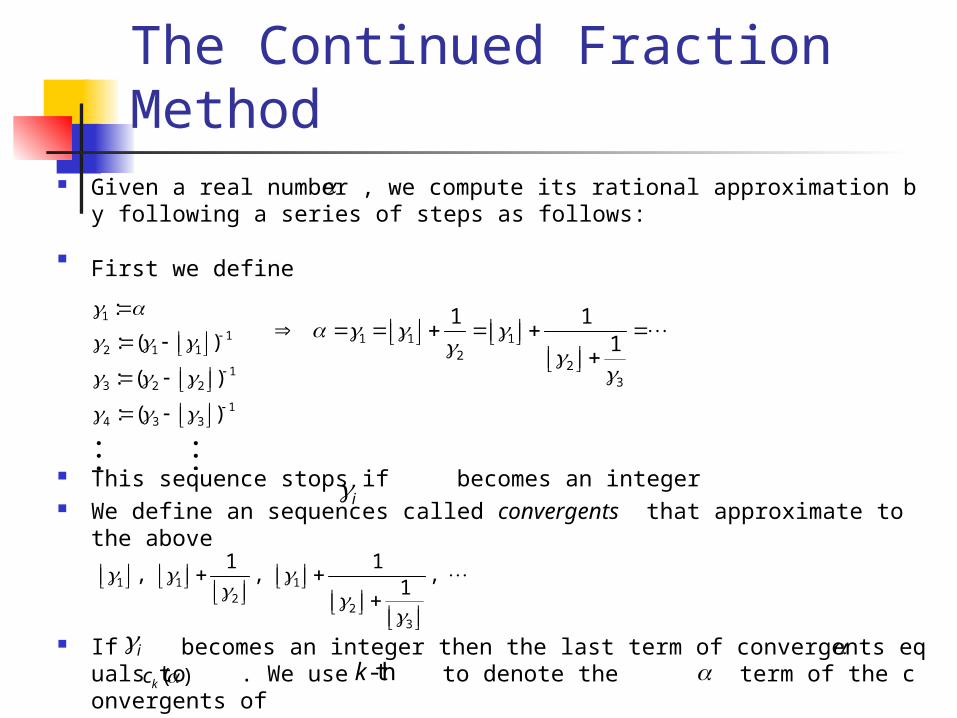
Given a real number , we compute its rational approximation by following a series of steps as follows:
First we define
This sequence stops if becomes an integer We define an sequences called convergents that approximate to the abov
e
If becomes an integer then the last term of convergents equals to . We use to denote the term of the convergents of
The Continued Fraction Method
1
12 1 1
13 2 2
14 3 3
:
: ( )
: ( )
: ( )
1 1 12
23
1 1
1
1 1 12
23
1 1, , ,
1
i
i ( )kc -thk
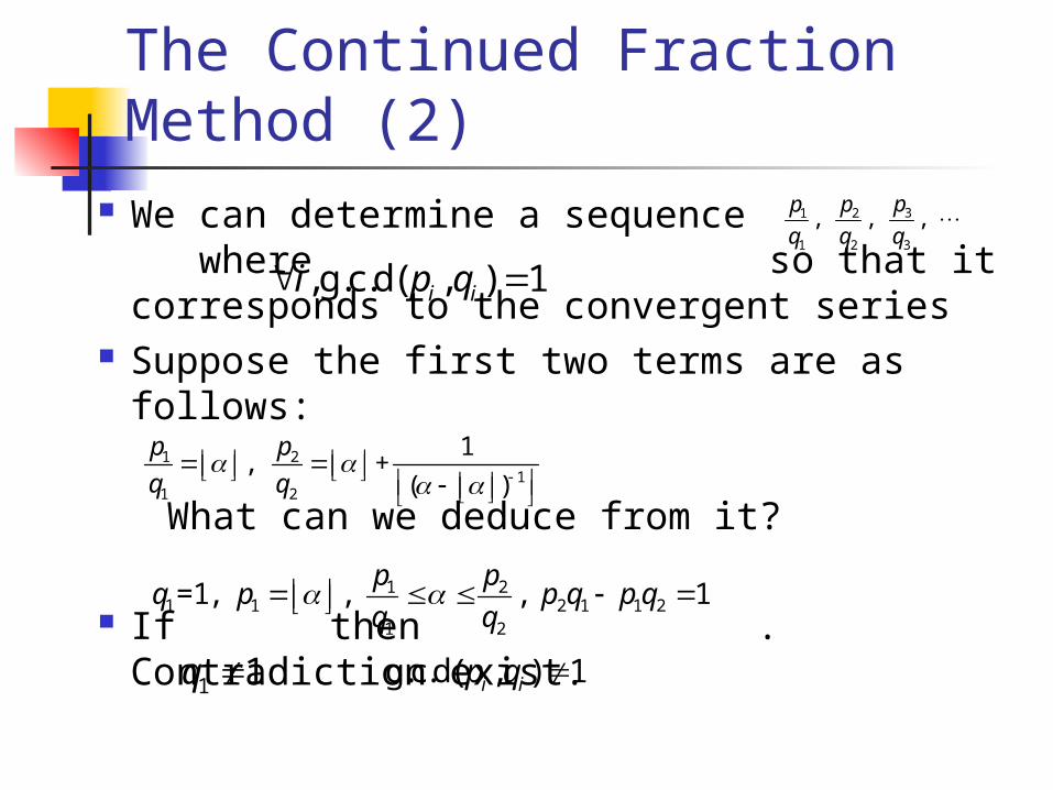
The Continued Fraction Method (2)
We can determine a sequence where so that it corresponds to the convergent series
Suppose the first two terms are as follows:
What can we deduce from it?
If then . Contradiction exist.
31 2
1 2 3
, , , pp p
q q q
1 21
1 2
1, +
( )
p p
q q
,g.c.d( , ) 1i ii p q
1 21 1 2 1 1 2
1 2
=1, , , 1p p
q p p q p qq q
1 1q g.c.d( , ) 1i ip q

Proof
21 11 1
2
1
1 1 1+ + +
{ } {{ } }( ) { }
1+ +{ }
{ }
p
q a
aa
2 11 1
2 1
1 2 22 1 1 2 1 1
12
1 12 2 1
1 1
( ) ( )
( ) ( )
( )
1( ) ( ) ( ( )
( )
p p
q q
q q qp q p q
q k
p q k k k
2 1 1 2
11)
1
k
p q p q

The Continued Fraction Method (3)
Suppose we have found nonnegative integers such that
This implies why?
1 1, , ,k k k kp q p q
11 1
1
, 1. Where is even.k kk k k k
k k
p pp q p q k
q q
1 1g.c.d( , ) g.c.d( , ) 1k k k kp q p q
1 1
1 1
1 1
1 1
1
Suppose g.c.d.( , ) 1
Let g.c.d.( , ) 1, , , g.c.d.( , ) 1
1
1
( ) 1
( 1) ( 1)
Contradiction exist
Similarly, we can prove g.c.d.( ,
k k
k k k k
k k k k
k k
k k
k k
k
p q
p q k p ak q bk a b
p q p q
akq p bk
k aq bp
k aq bp
p
1) 1kq

The Continued Fraction Method (4)
We find the largest integer such that
We define
If then the sequence stop, otherwise we find the largest such that
We define and so on…… We can repeat the iteration and find the sequence
It turns out that this sequence is the same as the sequence of convergents of real number !
t 1
1
k k
k k
p tp
q tq
1 1 1 1: ; :k k k k k kp p tp q q tq
1 1/k kp q t
1
1
k k
k k
p up
q uq
1 1 1 1 1 1( ) ( ) 1
Which implies g.c.d( , )=1 !k k k k k k k k k k k k k k
k k
p q p q p q tq p tp q p q p q
p q
2 1 2 1: ; :k k k k k kp p up q q uq
31 2
1 2 3
, , , pp p
q q q

Proof We use to denote the term with respect to
First we prove when Prove by induction
Then we prove
Prove by induction
1
1
11 ( ) ( )i i
i i
p qi
q p
( )i
i
p
q -thi
( ) ( )kk
k
pc
q
0 1

Some Properties ofSequence
Denominators are monotonically increasing
For any real numbers and with , one of the convergents satisfy the Dirichlet’s theorem
Proof: Let be the last convergent for which holds. Then
The sequence converge to Proof by induction
/i ip q
1 1 1
1 1 1 1
1 1k k k k k k
k k k k k k k k
p p p q p q
q q q q q q q q
1 2 3, , ,...q q q
12
1 1
1 1k k k
k k k k k k
p p p
q q q q q q
0,0 1 /i ip q
1 and 1p
qq q
/k kp q 1kq
1
1k
k k k k
p
q q q q
/i ip q

Algorithm of Continued Fraction Method
Initially . Suppose then we compute by
using the following rule: If k is even and , subtract times the second column of
from the first column; If k is odd and , subtract times the first column of
from the second column; The matrices is in the following form:
The found in this way are the same as in the convergents
Proved by induction
0
1
: 1 0
0 1
A
:k k
k k k
k k
A
1kA
0k /k k 1kA
0k /k k 1kA
1 1 2 3 2 3 4
1 1 2 3 2 3 4
1 1 2 3 2 3 4
1
1 0 , 0 , , ,
0 1 1
q q q q q q q
p p p p p p p
0 1 2, , ,...A A A
,k kp q ,k kp q

Time complexity of Continued Fraction Method Corollary. Given rational number , the continued fraction
method finds integers and as described in Dirichelet’s theorem in time polynomially bounded by the size of
Proved similar to Euclidean algorithm Theorem. Let be a real number, and let and be natural
numbers with . Then occurs as convergent for
Corollary. There exist a polynomial algorithm which, for given rational number and natural number M, tests if there exists a rational number with . If so, finds this rational number.
p q
0 p q2/ 1/ 2p q q /p q
/p q
2/ 1/ 2p q M

Summary Given a real number , there exist
a rational number with small that is close enough to
Continued fraction method compute a rational number that equals to if is a rational number. Otherwise converge to
The algorithm for continued fraction method is a polynomial Euclidean-like algorithm
/p q
q
/p q /p q

Basis Reduction in Lattices - Overview
Problem: Given a lattice (represented by its basis), finds a reduced “short” (nearly orthogonal) basis.
Applications: Finding a short nonzero vector in a lattice Simultaneous Diophantine approximation Finding the Hermite normal form Basis reduction has numerous applications in
cryptanalysis of public-key encryption schemes: knapsack cryptosystems, RSA with particular settings, and so forth

Basic Concepts Review Lattice. Given a sequence of vectors
, and a group we say generate if . We call a lattice and the basis of . In other words, a lattice can be seen as an integer linear combinations of its basis. It is a subset of the subspace generated by its basis.
A matrix can be seen as a sequence of column (row) vectors, therefore a lattice can be generated by columns (rows) of a matrix
1 2, ,..., ma a a1 2, ,..., ma a a
1 1 2 2 1... | ,...,m m ma a a 1 2, ,..., ma a a

Basic Concepts Review - 2 Let A and B both be a nonsingular matrix of order n, and whose column
both generate the same lattice , then and this is called the det of lattice . In other words, det is independent to chose of basis
Proof: Lemma 1: If B is obtained by interchanging two columns (rows) of A, th
en det B = -det A. Proof: Complicated (component-wise) proof by induction
Lemma 2: If A has two identical columns (rows), then det A = 0. Proof: Let A be a matrix with two identical rows, let B be a matrix constructe
d from A by interchanging these two column (rows). Then det B = det A because these two matrices are equal. However, from Lemma 1 we know that det B = -det A. So det B = det A = 0
Lemma 3: The determinant of an nxn matrix can be computed by expansion of any row or column.
Also called Laplace Expansion Theorem, component-wisely proved by Laplace.
Lemma 4: If B is obtained by multiplying a column (row) of A by k, then det B = k det A.
Proof. We can calculate det B by expanding the same column (row) of B as that of A, which yields det B = k det A.
det det A B

Basic Concepts Review - 3 Lemma 5: If A, B and C are identical except that the i-th colu
mn (row) of C is the sum of the i-th columns (rows) of A and B, then det C = det A + det B.
Proof. We can calculate det B by expanding the i-th column of C, then we can prove det C = det A + det B by using the distributivity of multiplication of matrices
Lemma 6: If B is obtained by adding a multiple of one column (row) i of A to another column (row) j, then det B = det A.
Proof. Let A’ be the matrix that constructed by replacing column (row) i of A to j, then det A’ = 0 because A’ has two identical columns. Matrix A, A’ and B satisfy Lemma 5 so that det B = det A + det A’ = det A
Lemma 7: If If B is obtained by elementary column operations from A, then |det B| = |det A|.
Proof. Directly from Lemma 1, 4 and 6.
From chapter 4, we know that if matrix A and B generate the same lattice then they have the same Hermite Normal Form by elementary column operations, therefore from Lemma 7 we have |det B| = |det A|.

Geometric Meaning of Determinant
The determinant of corresponds to the volume of the parallelepiped
Where is any basis for
Hadamard Inequality theorem:
When are orthogonal to each other, the equality holds.
We now have the lower bound of , what about the upper bound?
Hermite showed that Minkowski showed that
Schnorr proved that for each fixedthen there exist a polynomial algorithm finding a basis satisfying
1 1 2 2... | 0 1 for 1,...,n n ib b b i n
1,..., nb b
1 2det , where denotes the Euclidean norm Tnb b b x x x
1 2 nb b b
( 1) / 41 2 (4 / 3) det n n
nb b b
/ 21 2 (2 / ) det (2 / ) det n
n nb b b n V n e
1,..., nb b
0
( 1)1 2 (1 ) det n n
nb b b

Basis Reduction Theorem A matrix is called positive definite if
There exist a polynomial algorithm which, for given positive definite rational matrix D, finds a basis
for the lattice satisfying ‖b1‖ ‖b2‖…‖bn‖≤ where ‖x‖
We prove this theorem by showing the LLL algorithm
for all 0, 0Tx x Ax
1 2, ,..., nb b b n( 1) / 42 det n n D
: Tx Dx

The Lenstra, Lenstra and Lovász Algorithm We construct a series of basis for as follows: The first basis is the unit basis. We construct the next basis inductively using the following
steps: 1. Denote as the matrix with columns , we
calculate
2.
3. Choose, if possible, an index i such that ‖b2*‖2>2‖b*
i+1‖2. Exchange bi and bi+1, and start with step 1 again. If no such i exists, the algorithm stops.
n
iB 1 2, ,..., nb b b* 1
1 1 1 1( )T Ti i i i i i ib b B B DB B Db
1 1
* * *1 1
for 2,...,
for 1, 2,...,1
1/ 2
i i i i
i i j j
i n
j i i
b b b b
b b b

The Lenstra, Lenstra and Lovász Algorithm - Continued The LLL algorithm is an approximation of the Gra
m-Schmidt orthogonalization process which finds a orthogonal basis in a subspace of
The LLL algorithm terminates in polynomial time, with intermediate numbers polynomially bounded by the size of D
Complicated proof see p.68 – p.71
n

Finding a Short Nonzero Vector in a Lattice In 1891, Minkowski proved a classical result: any n-dimensional latti
ce contains a nonzero vector b with
where denotes the volume of the n-dimensional unit ball. However, no polynomial algorithm finding such a vector b is known.
With the basis reduction method, by taking the shortest vector one can find a “longer short vector” in a lattice, which satisfy
However, this vector is generally not the shortest one in the lattice
The CVP (Closest Vector Problem): “Given a lattice and vector a, find b with (any kind of) norm of b-a as small as possible” is proven to be NP-complete
The SVP (Shortest Nonzero Vector Problem): “Given a lattice, finding a vector in the lattice as small as possible” is even proven to be NP-hard to approximate within some constant [Dan 2001]
1/det 2( ) n
n
bV
nV
( 1) / 4 1/2 (det )n n nb D
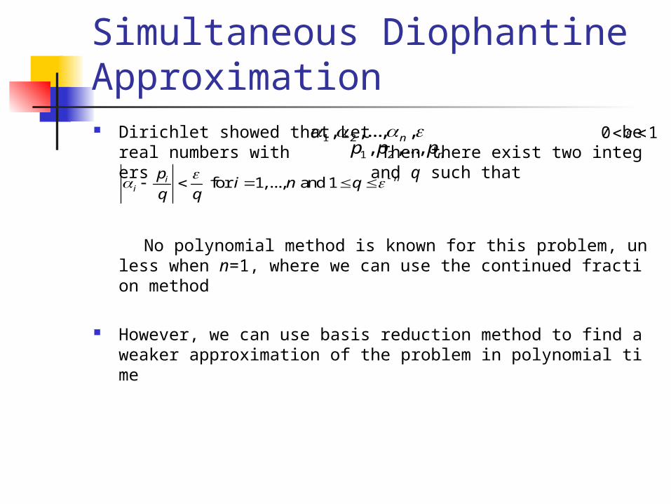
Simultaneous Diophantine Approximation Dirichlet showed that Let be real numbers with Then
there exist two integers and q such that
No polynomial method is known for this problem, unless when n=1, where we can use the continued fraction method
However, we can use basis reduction method to find a weaker approximation of the problem in polynomial time
0 1 1 2, ,..., ,n 1 2, ,..., np p p
for 1,..., and 1 nii
pi n q
q q

Finding the Hermite Normal Form Given a matrix A, we can use basis reduction method to calculate ve
ctor and record it in such a way that it can be transform to Hermite Normal Form by elementary column operations
Some of the other applications Lenstra’s Integer Linear Programming algorithm Factoring polynomials (over rationals) in polynomial time Breaking cryptographic codes Disproving Mertens’ conjecture Solving low density subset sum problems
1 2, ,..., nb b b
Summary The continued fraction method for ap
proximating one real number by rational numbers
Lovász’s basis reduction method for finding a short basis in a lattice
Applications

Thank you


