56
DIPimage User Manual dr. ir. Cris L. Luengo Hendriks prof. dr. ir. Lucas J. van Vliet dr. dipl. phys. Bernd Rieger dr. ir. Michael van Ginkel ing. Ronald Ligteringen
| Date post: | 03-Jan-2016 |
| Category: |
Documents |
| Upload: | escuela-futbol-novo-chiclana |
| View: | 187 times |
| Download: | 3 times |

DIPimage User Manual
dr. ir. Cris L. Luengo Hendriks
prof. dr. ir. Lucas J. van Vliet
dr. dipl. phys. Bernd Rieger
dr. ir. Michael van Ginkel
ing. Ronald Ligteringen

Quantitative Imaging Group,Faculty of Applied Physics, DelftDelft University of Technology June 9, 2005

Contents
1 Introduction 1
1.1 The DIPimage toolbox . . . . . . . . . . . . . . . . . . . . . . . . . . . . . . . 1
1.2 The DIPlib library . . . . . . . . . . . . . . . . . . . . . . . . . . . . . . . . . 1
1.3 Image Processing . . . . . . . . . . . . . . . . . . . . . . . . . . . . . . . . . . 2
1.4 Documentation Conventions . . . . . . . . . . . . . . . . . . . . . . . . . . . . 2
1.5 Acknowledgements . . . . . . . . . . . . . . . . . . . . . . . . . . . . . . . . . 2
2 Installing DIPimage 3
2.1 Windows Installation . . . . . . . . . . . . . . . . . . . . . . . . . . . . . . . . 3
2.2 UNIX Installation . . . . . . . . . . . . . . . . . . . . . . . . . . . . . . . . . 4
2.3 MacOS X Installation . . . . . . . . . . . . . . . . . . . . . . . . . . . . . . . 5
2.3.1 Using MATLAB on MacOS X . . . . . . . . . . . . . . . . . . . . . . . 5
2.3.2 Slightly related tips... . . . . . . . . . . . . . . . . . . . . . . . . . . . 6
3 Getting Started 7
3.1 Starting the GUI . . . . . . . . . . . . . . . . . . . . . . . . . . . . . . . . . . 7
3.2 Loading and Displaying an Image . . . . . . . . . . . . . . . . . . . . . . . . . 7
3.3 Pre-processing the Image . . . . . . . . . . . . . . . . . . . . . . . . . . . . . 8
3.4 Measuring . . . . . . . . . . . . . . . . . . . . . . . . . . . . . . . . . . . . . . 9
3.5 Where to Go from Here . . . . . . . . . . . . . . . . . . . . . . . . . . . . . . 11
4 The dip image Object 12
4.1 Creating a dip image Object . . . . . . . . . . . . . . . . . . . . . . . . . . . 12
4.2 Displaying dip image Objects . . . . . . . . . . . . . . . . . . . . . . . . . . . 13
4.3 Operations on dip image Objects . . . . . . . . . . . . . . . . . . . . . . . . . 13
4.4 Indexing Pixels . . . . . . . . . . . . . . . . . . . . . . . . . . . . . . . . . . . 14
4.5 Dimensions . . . . . . . . . . . . . . . . . . . . . . . . . . . . . . . . . . . . . 15
4.6 Image Arrays . . . . . . . . . . . . . . . . . . . . . . . . . . . . . . . . . . . . 16
4.7 Tensor Images . . . . . . . . . . . . . . . . . . . . . . . . . . . . . . . . . . . . 16
4.8 Color Images . . . . . . . . . . . . . . . . . . . . . . . . . . . . . . . . . . . . 17
III

IV Contents
4.9 A Note on the end Method in Indexing . . . . . . . . . . . . . . . . . . . . . . 18
4.10 Special Functions . . . . . . . . . . . . . . . . . . . . . . . . . . . . . . . . . . 18
4.11 Review of the Differences Between a dip image and a MATLAB Array . . . . 22
5 The dip measurement Object 24
5.1 Extracting Measurement Data . . . . . . . . . . . . . . . . . . . . . . . . . . 24
5.2 Other Information on the dip measurement Object . . . . . . . . . . . . . . . 24
5.3 Combining Measurement Data . . . . . . . . . . . . . . . . . . . . . . . . . . 25
5.4 Converting a dip measurement Object to a dataset Object . . . . . . . . . . 25
5.5 Creating a dip measurement Object with Your Own Data . . . . . . . . . . . 26
5.6 Backwards Compatibility . . . . . . . . . . . . . . . . . . . . . . . . . . . . . 26
6 Figure Windows 27
6.1 The Figure Window Menus . . . . . . . . . . . . . . . . . . . . . . . . . . . . 27
6.2 Using the Mouse in Figure Windows . . . . . . . . . . . . . . . . . . . . . . . 28
6.3 Using the Keyboard in Figure Windows . . . . . . . . . . . . . . . . . . . . . 29
6.4 Linking Variables with Figure Windows . . . . . . . . . . . . . . . . . . . . . 30
6.5 Setting the Position of Figure Windows . . . . . . . . . . . . . . . . . . . . . 30
7 Toolbox Functions 32
7.1 The GUI: dipimage . . . . . . . . . . . . . . . . . . . . . . . . . . . . . . . . 32
7.2 The dipshow Function . . . . . . . . . . . . . . . . . . . . . . . . . . . . . . . 32
7.3 Figure Window Support: dipmapping . . . . . . . . . . . . . . . . . . . . . . 33
7.4 Figure Window Support: diptruesize . . . . . . . . . . . . . . . . . . . . . . 33
7.5 Figure Window Support: diptest, dipzoom, et al. . . . . . . . . . . . . . . . 34
7.6 Figure Window Support: diplink . . . . . . . . . . . . . . . . . . . . . . . . 34
7.7 Creating, Linking and Clearing Figure Windows: dipfig and dipclf . . . . 35
7.8 Toolbox Preferences: dipsetpref and dipgetpref . . . . . . . . . . . . . . . 35
7.9 Interactive Tools: dipcrop, dipgetcoords, et al. . . . . . . . . . . . . . . . . 36
7.10 Image Processing Functions . . . . . . . . . . . . . . . . . . . . . . . . . . . . 36
7.11 Adding Functions to the GUI . . . . . . . . . . . . . . . . . . . . . . . . . . . 36
7.12 Automatic Parameter Parsing . . . . . . . . . . . . . . . . . . . . . . . . . . . 41
8 Customizing the DIPimage Environment 42
8.1 Figure Windows . . . . . . . . . . . . . . . . . . . . . . . . . . . . . . . . . . 42
8.2 Graphical user Interface . . . . . . . . . . . . . . . . . . . . . . . . . . . . . . 42

DIPimage User Manual V
8.3 Initialization File . . . . . . . . . . . . . . . . . . . . . . . . . . . . . . . . . . 43
8.4 Other Settings . . . . . . . . . . . . . . . . . . . . . . . . . . . . . . . . . . . 43
9 Low-level DIPlib Interface 48
9.1 The Setup . . . . . . . . . . . . . . . . . . . . . . . . . . . . . . . . . . . . . . 48
9.2 Calling DIPlib Functions . . . . . . . . . . . . . . . . . . . . . . . . . . . . . . 48
9.3 Example Function Call . . . . . . . . . . . . . . . . . . . . . . . . . . . . . . . 49

VI

Chapter 1
Introduction
1.1 The DIPimage toolbox
MATLAB is a software package designed for (among other things) data processing. It containsa huge amount of numerical algorithms, and very good data-visualization abilities. This makesit adequate for image processing. However, MATLAB’s virtues do not end there. It is alsoan ideal tool for rapid prototyping, since it handles a compact but simple notation and it isvery easy to add functions to it. The drawback is that MATLAB, since it is an interpretedlanguage, is slow for some constructs like loops; it also is not very efficient with memory (forexample, all MATLAB data uses 8-byte floats). This makes it a bit less useful beyond theprototyping stage.
DIPimage is a MATLAB toolbox for doing image processing, and is based on the image-processing library DIPlib. It is meant as a tool for research as well as teaching image pro-cessing at various levels. It is not meant as an industrial image-processing package, whichshould heavily depend on speed and memory-efficiency. Instead, this toolbox is made withuser-friendliness, ease of implementation of new features, and compactness of notation inmind.
Most arithmetic operations are done by MATLAB. However, implementing image-processingfilters usually requires several nested loops (depending on the dimensionality of the inputdata), which is not very efficient. Therefore, we based this toolbox on DIPlib. It provides allfiltering and transform functions and is the heart of the DIPimage toolbox.
1.2 The DIPlib library
DIPlib is a scientific image-processing library written in C. It contains a large number offunctions for processing and analyzing multi-dimensional image data. The library providesfunctions for performing transforms, filter operations, object generation, and statistical anal-ysis of images. It is also very efficient (with both memory and time).
The MATLAB interface to DIPlib is a simple “glue” layer, which allows calling the C functionsin the library by converting the MATLAB data to a form used by the library. Only a fewfunctions have added functionality in the interface. Using these functions therefore is muchlike using the C functions directly. This is not adequate for the beginning image analyst, whois better off using the DIPimage toolbox functions instead.
More information on DIPlib can be found at:http://www.qi.tnw.tudelft.nl/DIPlib/.
1

2 Chapter 1. Introduction
1.3 Image Processing
This manual is meant as an introduction and reference to the DIPimage toolbox, not as atutorial on image processing. Although Chapter 3 shows some image-processing basics, itis not complete. We refer to “The Fundamentals of Image Processing”, an online image-processing course, which can be found at:http://www.qi.tnw.tudelft.nl/DIPlib/docs/FIP.pdf.
1.4 Documentation Conventions
The following conventions are used throughout this manual:
• Example code: in typewriter font
• File names and URLs: in typewriter font
• Function names/syntax: in typewriter font
• Keys: in bold
• Mathematical expressions: in italic
• Menu names, menu items, and controls: “inside quotes”
• Description of incomplete features: in italic
1.5 Acknowledgements
DIPlib was written mainly by Michael van Ginkel, Geert van Kempen, Cris Luengo andLucas van Vliet; the MATLAB interface to DIPlib was written by Cris Luengo, with helpfrom Michael van Ginkel.
The DIPimage toolbox was written mainly by Cris Luengo, Lucas van Vliet, Bernd Riegerand Michael van Ginkel. Tuan Pham, Kees van Wijk, Judith Dijk, Geert van Kempen andPeter Bakker have contributed functionality.
DIPlib and the DIPimage toolbox are being developed at the Quantitative Imaging Group,Delft University of Technology. Lucas van Vliet is the project supervisor.
Chapter 2
Installing DIPimage
This toolbox requires MATLAB 5.3 or later. Some functionality is only available on MATLAB6 or on the Windows platform, but this is an exception. The bulk of the toolbox is platform-independent.
2.1 Windows Installation
If you have an earlier version of DIPimage installed, it is important that you remove it beforeinstalling this version. Either delete or rename the whole directory. Make sure to removeor rename the files libdip.dll, libdipio.dll and libdml.dll, if they are present in theMATLAB\bin\ or the MATLAB\bin\win32\ directory, or the system directory.
Note: depending on the version of DIPimage you previously had, it is possible that youdon’t have the three files named above. Instead, you will have three files named DIPlib.dll,dipIO.dll and dipmex.dll. These files won’t interfere with a new installation.
Unzip the distribution file dipimage.zip to a new directory (say, C:\newdir\). It will gener-ate two sub-directories: C:\newdir\dipimage\ and C:\newdir\bin\. The first one containsthe MATLAB toolbox, the second one the DIPlib library and two support libraries. Thesystem (Windows, not MATLAB) must be able to find these library files. This can be ac-complished one of the following ways:
• Add the C:\newdir\bin\ directory to the PATH environment variable. Environmentvariables can be set through the ‘System’ control panel. (If this doesn’t mean anythingto you, use one of the other methods.)
• Copy the three files (libdip.dll, libdipio.dll and libdml.dll) from theC:\newdir\bin\ directory to MATLAB’s bin directory:
– if you have MATLAB 5: C:\MATLABR11\bin\.– if you have MATLAB 6: C:\MATLABR12\bin\win32\.
• Copy these three files to the system directory (C:\WINNT\system32\). This option isbetter than the previous one if you are also going to use DIPlib independently fromMATLAB.
You also might want to unzip the images file images.zip to the same directory. It will createa directory C:\newdir\images\ with some default images.
3

4 Chapter 2. Installing DIPimage
To start using DIPimage, do the following in MATLAB:diproot = ’C:\newdir’;addpath([diproot,’\dipimage’],...
[diproot,’\dipimage\diplib’],’-begin’)dip_initialisedipsetpref(’imagefilepath’,[diproot,’\images’])
(make sure to substitute ’C:\newdir\’ for the name of the directory where you unzipped thedistribution file). This will add the DIPimage toolbox and low-level DIPlib interface to thebeginning of the path, initialize DIPlib and set the default directory where DIPimage willlook for images.
You can add these lines to your startup.m file, which should be in your working directory.That way, DIPimage will be ready to use each time you start MATLAB.
Optionally, you can add these directories to your path too:[diproot,’\dipimage\demos’][diproot,’\dipimage\aliases’]
The first one contains a few demos that show how to use different features of the toolbox.The second one contains aliases for functions that have changed their names since the firstrelease. You will need these aliases if you have written M-files that use any of the functionsthat have changed names (however, we recommend you change your functions to use the newnames).
2.2 UNIX Installation
If you already have a version of DIPimage installed, rename the directory it is in, so that youwill still have the old version if the installation of the new version fails. Untar the distributionfile. It will create a directory dip/ with a number of subdirectories. If you untarred the filein the directory /something/, you now have a directory /something/dip/. To get DIPimagerunning, there are a number of things that you must do:
1. MATLAB must be told where it can find DIPlib, a shared library, that is used byDIPimage. You can do this by creating the environment variable LD LIBRARY PATH, orextending it if it already exists. As the name suggests, it holds a collection of paths.The entries are separated by colons, i.e. ‘:’. Which entry you should add, depends onthe type of machine you are working on:
• On Solaris add: /something/dip/SunOS/lib/
• On Linux add: /something/dip/Linux/lib/
2. If you did not do so before: download the separate tar or zip file containing some testimages. Install them somewhere on your system. Let us assume that you installed themin /herebeimages/.

DIPimage User Manual 5
3. Add the following lines to your startup.m (preferably in $HOME/matlab/):diproot = ’/something/dip/toolbox’;addpath([diproot,’/dipimage’],...
[diproot,’/diplib’],’-begin’)dip_initialisedipsetpref(’imagefilepath’,’/herebeimages’)
This will add the DIPimage toolbox and low-level DIPlib interface to the beginning of thepath, initialize DIPlib and set the default directory where DIPimage will look for images.
Optionally, you can add these directories to your path too:[diproot,’/dipimage/demos’][diproot,’/dipimage/aliases’]
The first one contains a few demos that show how to use different features of the toolbox.The second one contains aliases for functions that have changed their names since the firstrelease. You will need these aliases if you have written M-files that use any of the functionsthat have changed names (however, we recommend you change your functions to use the newnames).
2.3 MacOS X Installation
For installation of DIPimage on the MacOS X platform you must use the unix shell andfollow the instructions as described in Section 2.2. The entry for this platform will be:
• On MacOS X add: /something/dip/Darwin/lib/
NOTE: as it turns out, in some occasions Darwin (the unix of MacOS X) does not lookat LD LIBRARY PATH. As a result the DIPlib libraries cannot be found during the startup ofMATLAB. As a workaround of this problem copy all files from /something/dip/Darwin/lib/to /usr/lib/!
2.3.1 Using MATLAB on MacOS X
The following is for the brave of heart. Follow these tips at your own risk!
When using the default installation of MATLAB for MacOS X the script will install Orobox-OSX as well. This window manager works together with XDarwin. As it turns out, the newX11 distribution from Apple is much faster then XDarwin and also comes included with itsown window manager. You can change the startup script of MATLAB removing the startupof OroborOSX and add the startup of X11.
Note that as of Matlab R13 X11 is used and these steps are no longer needed!
Depending on were you installed MATLAB the startup script can be found somewhere here:
/Applications/MATLAB6p5/bin/LaunchMATLAB.app/Contents/launch\_matlab.sh

6 Chapter 2. Installing DIPimage
Below is this modified script to use X11 (make sure to modify the paths to your settings):\#!/bin/sh
if [ "‘ps axc | grep X11‘" ]; thensleeptime=30
else/Applications/X11.app/Contents/MacOS/X11 \&sleeptime=35
fi
cd ../..
bin/mac/setsid bin/matlab -desktop -display :0.0 \&
\# Bounce to let user know MATLAB is starting up./bin/sleep \$sleeptime
2.3.2 Slightly related tips...
During the process of porting DIPlib to MacOS X I found it extremely handy to use the’Fink’ project. This package manager allows you to conveniently select from a vast amountof precompiled binary packages and to install them. For more information check:http://fink.sourceforge.net/.
Installing of MacOS X on a non-G3/G4 machine can be tried with XPostFacto. Rememberto start off with at least MacOS 9.1!. For more information check:http://eshop.macsales.com/OSXCenter/XPostFacto/.

Chapter 3
Getting Started
To show you around DIPimage, we will work through a simple image-processing application.Not all steps will be written out explicitly, since it is our goal to make you understand whatis going on, and not to have you copy some commands and stare in amazement at the result.
The goal of this application is to do some measurements on an image of some rice grains,then analyze these measurements.
3.1 Starting the GUI
Type the following command at the MATLAB prompt:
dipimage
This should start the DIPimage GUI. A new window appears to the top-left of the screen,which contains a menu bar. Spend some time exploring the menus. When you choose one ofthe options, the area beneath the menu bar should change into a dialog box that allows youto enter the parameters for the filter you have chosen. See also Sections 7.1 and 8.2 for moreinfo on the GUI.
3.2 Loading and Displaying an Image
Before you can use these functions, you first need to load some image. The first menu iscalled “File I/O”, and its first item “Read image (readim)”. Select it. Press the “Browse”button, and choose the file rice.tif. Change the name for the output variable from ans toa, then press the “Execute” button. Two things should happen:
1. The image ‘rice’ is loaded into the variable a, and displayed to some figure window:
7

8 Chapter 3. Getting Started
2. The following lines (or something very similar) appear in the command window:>> a = readim(’c:\matlab\toolbox\dipimage\images\rice.tif’,’’)Displayed in figure 1
This is to show you that the same would have happened if you would have typed that commanddirectly yourself, without using the GUI. Try typing this command:
a = readim(’rice’)
The same image should be loaded into the same variable, and again displayed to some window.Note that we left off the ’.tif’ ending of the filename. readim can find the file without youhaving to specify the extension. We also didn’t use the second argument to the readimfunction, since ’’ is the default value. Finally, by not specifying a path to the file, we askedthe function to look for it either in the current directory or in any of the directories specifiedby the ImageFilePath setting (see Section 8.4).
To avoid having the image displayed in a window automatically, add a semicolon to the endof the command:
a = readim(’rice’);
3.3 Pre-processing the Image
You will have noticed the heavy background shading in this image. If we try to segment itdirectly, the results will be unsatisfactory (as you can try out later). Let’s do some backgroundcorrection. The idea is to use a low-pass filter that removes the objects while keeping theslow change in the background. Choose “Filters” and “Gaussian filter”. Select a as the inputimage, and choose a name for your background image (we use bg). Finally, choose a suitablevalue for the filter parameter, such that the objects are removed and the background shadingis left. Try different settings until you are satisfied with the result.
Once we have the background image, we can subtract it from the original image. It is veryeasy to do arithmetic with images in MATLAB. Type
a = a - bg
The new image should be displayed to a figure window, but it looks very dark. This isbecause the pixels have lower values now, some even have negative values. By default, imagesare displayed by mapping the value 0 to black, and the value 255 to white. You can change

DIPimage User Manual 9
this by choosing a different mapping mode. Open the “Mappings” menu on the figure window,and choose “Linear stretch” (try out the other modes too).
The “Actions” menu allows you to choose what the mouse should do on the figure window.Select “Pixel testing”, and press the mouse button while pointing somewhere in the image(keep the button down). The figure caption changes to show the coordinates of the mousein the image and the value of the pixel at those coordinates. Try moving the mouse whileholding the button down. Another option on the “Actions” menu (“Zoom”) is used to zoomin on an image. Try it out too. See Chapter 6 for more information on the figure windows.
The next step is to segment the image. We need to find some threshold that distinguishes thegrains of rice from the background. To find it, we can examine the histogram of the image.Choose “Histogram” on the “Statistics” menu, or type
diphist(a,[])
The graph shows two peaks, one for the background, one for the objects. Find a valuein between for the threshold. To do the segmentation, compare all pixel values with thethreshold, which can be done in this way:
b = a > 20
This results in a binary image (logical image, containing values of “true” and “false”, codedas 1 and 0), with ones at the pixels that belong to the objects.
The final step is to remove the grains that do not completely lie inside the image. We cando this using a binary operation. Find and execute the “Remove edge objects” function inthe menu system. What it does is the same as the bpropagation function, with an emptyimage as a seed image, and the edge condition set to 1. To create an empty seed image usethe newim function. Thus, these two commands are equivalent:
b = b - bpropagation(newim(b,’bin’),b,0,2,1)b = brmedgeobjs(b,2)
3.4 Measuring
Before we can start measuring, it is convenient to have a label image. Select the “Labelobjects” item on the “Transforms” menu, and select the new object image as the input. Theresult (name the image lab) is a labeled image where the pixels belonging to each object havea different value. In the window of the new image, select the “Labels” mapping. Now each

10 Chapter 3. Getting Started
grey-value gets a different color. Examine the pixel values to see how the objects are labeled.
Now do the measuring. We will measure the object area in pixels (’size’) and the Feretdiameters (’feret’), which are the largest and smallest diameters, and the diameter perpen-dicular to the smallest diameter.
data = measure(lab,[],’size’,’feret’);
measure returns an object of type dip measurement, which is explained further in Chapter 5.Leaving the semi-colon off the previous command, the complete measurement results are dis-played at the command prompt. Furthermore, data(1) is the measurement results for objectwith label 1, data.feret is an array containing all the Feret diameters, and data(1).feretare the Feret diameters for object number 1.
To extract the measurements done on all objects and put them in an array, typeferet = data.feret;sz = data.size;
This gives us arrays with the measured data. MATLAB allows all kinds of statistics andanalysis on these arrays. For example, mean(sz) gives the mean grain area.
We will use scatter to find some correlation between the diameters and the area of thegrains. Let’s start by plotting the length of the grains against their width:
figure; scatter(feret(1,:),feret(2,:))
Apparently, they are mostly unrelated. Let’s try a relation between the length and the surfacearea:
scatter(feret(1,:),sz)
These appear to be more related, but, of course, the area also depends on the width of thegrains. If we assume that the grains are elliptic, we know that the area is 1
4πd1d2. Let’s plotthe calculated area against the measured area:
scatter(sz,pi*feret(1,:).*feret(2,:)/4)

DIPimage User Manual 11
Wow! That is a linear relation. We can add a line along the diagonal to see how much theratio differs from 1 (the other commands are to make the figure look more pretty):hold on , plot([180,360],[180,360],’k--’)axis equal , box onxlabel(’object area (pixels^2)’)ylabel(’\pi\cdota\cdotb (pixels^2)’)
The actual slope can be computed by:
f = sz’\calc’
(this is the lest-squares solution to the linear equation sz’*f = calc’; the apostrophes trans-pose the vectors to create column vectors).
3.5 Where to Go from Here
If you are new to MATLAB, it would be a good idea to read the “Getting Started withMATLAB” manual. If you are new to image processing, you can read “The Fundamentals ofImage Processing”, an online image-processing course, which can be found at:http://www.qi.tnw.tudelft.nl/DIPlib/docs/FIP.pdf.
Before you start using this toolbox, we recommend that you read Chapter 4 (at least Sec-tion 4.11). It contains very important information on the dip image object and its usage.Since it is not the same as a regular MATLAB array, it can be a bit confusing at first.

Chapter 4
The dip image Object
Images used by this toolbox are encapsulated in an object called dip image. Objects of thistype are unlike regular MATLAB arrays in some ways, but behave similarly most of the time.This chapter explains the usage of these objects.
4.1 Creating a dip image Object
To create a dip image object, the function dip image must be used. It converts any numericarray into an image object. The optional second argument indicates the desired data typefor the image. The pixel data will be converted to this type if possible, or else an error willbe generated (for example, it is illegal to convert complex data to a real type, since there aremany ways this can be accomplished; it is necessary to do this explicitly). The valid datatypes are listed in Table 4.1. This table also lists some alternative names that are mapped tothe names on the left; these are just to make specifying the data type easier.1
For example,
a = dip_image(a,’sfloat’);
will convert the data in a to single (4-byte) floats before creating the dip image object.The variable a now behaves somewhat differently than you might be used to. The followingsections explain its behavior.
There are also some commands to create an image from scratch. newim is equivalent to thezeros function, but returns a dip image object.
a = newim(256,256);
creates an image with 256x256 pixels set to zero. If b is an object of type dip image, then
a = newim(b);
creates an image of the same size (this is the same as newim(size(b))). The functions xx,yy, zz, rr and phiphi all create an image containing the coordinates of its pixels, and canbe used in formulas that need them. For example, rr(256,256)<64 creates a binary imagewith a disk of radius 64. The expression
a = (yy(’corner’))*sin((xx(’corner’))^2/300)
generates a nice test pattern with increasing frequency along the x-axis, and increasing am-plitude along the y-axis. All these functions have 256x256 pixels as the default output size,and allow as a parameter either the size of an image, or an image whose size is to be copied.
1Note that these are the names of some additional DIPlib data types not used under MATLAB, the namesMATLAB uses for the data types, and some generalizations of the other names.
12

DIPimage User Manual 13
Table 4.1: Valid data types for the dip image object.Name Description Other allowed namesbin binary (in 8-bit integer) bin8, bin16, bin32uint8 8-bit unsigned integeruint16 16-bit unsigned integeruint32 32-bit unsigned integer uintsint8 8-bit signed integer int8sint16 16-bit signed integer int16sint32 32-bit signed integer int, int32sfloat single precision float float, singledfloat double precision float doublescomplex single precision complexdcomplex double precision complex complex
For example, a*xx(a) is an image multiplied by its x-coordinates.
Images can have any dimensionality, including 0 and 1, which are not allowed in MATLABarrays. A 1-element numeric array is a special case of a two-dimensional array, whereas a1-pixel image is seen as a zero-dimensional image. This has repercussions in the possiblereturn values of size and ndims. For example, size will return an empty array for a zero-dimensional image, instead of the array [1,1]. For more information on image dimensionality,see Section 4.5.
4.2 Displaying dip image Objects
When a MATLAB command does not end with a semicolon, the display method is called forthe resulting values, if any. This method defaults to calling the disp method, which displaysall the values in matrices. For the dip image objects, the display method has been overloadedto call dipshow instead; dipshow displays the image in a figure window (see Section 7.2 formore information on this function). There is an exception for zero-dimensional and emptyimages, for which display always calls disp, and which will show information on the image.
The disp method shows only the image size and data type instead. If you want displayto call disp instead of dipshow, you can change the ’DisplayToFigure’ preference usingdipsetpref (see Sections 7.8 and 8.4).
4.3 Operations on dip image Objects
All mathematical operations have been overloaded for the dip image object. The matrixmultiplication (*), which is meaningless on images, does a pixel-by-pixel multiplication, justas the array multiplication (.*). The same applies to the other matrix operations. Relationaloperations return binary images. Binary operations on non-binary images treat any non-zerovalue in those images as true and zero as false. For example, to do a threshold we do notneed a special function, since we have the relational operators:
b = a > 100;

14 Chapter 4. The dip image Object
Table 4.2: Arithmetic functions defined for objects of type dip image(image in, image out).abs acos angle asin atan atan2besselj ceil conj cos erf expfix floor imag log log10 log2mod phase pow10 pow2 real roundsign sin sqrt tan xor
Table 4.3: Arithmetic functions defined for objects of type dip image (image in, scalar out).all any max mean median minmod percentile std sum
A double threshold would be (note MATLAB’s operator precedence):
b = a > 50 & a < 200;
A note is required on the data types of the resulting images. The “higher” data type alwaysdetermines this result, but we have chosen never to return an integer type after any arithmeticoperation. Thus, adding two integer images will result in a 4-byte floating-point image; an8-byte floating-point (double) image is returned only if any of the two inputs is double.
Many of the arithmetic functions have also been defined for objects of type dip image (seeTables 4.2 and 4.3 for a complete listing). The basic difference between these and theirMATLAB counterpart is that they work on the image as a whole, instead of on a per-columnbasis. For example, the function sum returns a row vector with the sum over the columns whenapplied to a numeric matrix, but returns a single number when applied to an image. Besidesthese, there are some other functions that are only defined for objects of type dip image.See Section 4.10 to learn about these functions. That section also lists some functions thatbehave differently than usual when applied to images.
4.4 Indexing Pixels
In image processing, it is conventional to index images starting at (0,0) in the upper-rightcorner, and have the first index (usually x), index into the image horizontally. Unfortunately,MATLAB is based on matrices, which are indexed starting at one, and indicating the rownumber first. By encapsulating images in an object, we were allowed to redefine the indexing.We chose not to follow MATLAB’s default indexing method. This might be confusing at first,and special care must be taken to check the class of a variable before indexing.
dip image objects are indexed from 0 to end in each dimension, the first being the horizontal.It is, of course, also possible to index using a single index, in which case, following MATLAB’sdefault behavior, the indices increase in the vertical direction, but start at 0 (i = y+x·height).The size function also returns the image width as the first number in the array.
Any portion of a dip image object, when extracted, is still a dip image object, even if itis just a single pixel. To get a numeric array out of an image, use the double function (ordip array, see Section 4.10). Thus, to get the value of a pixel in an image, type
b = double(a(0,0));

DIPimage User Manual 15
Table 4.4: Dimension manipulation functions.cat flipdim fliplr flipud permute repmatreshape rot90 shiftdim squeeze
Any numeric type can be assigned into a dip image object, without changing the image datatype (that is, the element assigned into the image is converted to the image data type). Forexample,
a(:,0) = 0;
sets the top row of the image in a to 0. Note that indexing expressions can become ascomplicated as you like. For example, to sub-sample the image by a factor 3, we could write
a = a(1:3:end,1:3:end);
Finally, it is also possible to index using a mask image. Any binary image (or logical array)can be used as mask, but it must be of the same size as the image into which is being indexed.For example,
a(m) = 0;
sets all pixels in a, where m is one, to zero. A very common expression is of the form
a(a<0) = 0;
(which sets all negative pixels to zero).
Note that the expression a(m) above returns a one-dimensional image, with all pixels selectedby the mask. Also, the expression a(:,0) does not return a 1D image, but a 2D image witha height of 1 (see Section 4.5). To obtain a 1D image use squeeze(a(:,0)).
4.5 Dimensions
The image in a dip image object can have any number of dimensions. As in MATLAB,operations between two images require that both images have the same number of dimensions,as well as the same size. There is only one exception to this rule.
In MATLAB, dimensions with size 1 are called singleton dimensions. Singleton dimensionsare always preserved, except at the end of the arrays. Thus, an array of size 4x1x6x1 is thesame as an array of size 4x1x6. This is not the case for objects of type dip image. Thesehave all singleton dimensions preserved. However, it is possible to do arithmetic operationsbetween two images with different number of trailing singleton dimensions (e.g. between twoimages with sizes 4x6x1 and 4x6). This is the exception to the rule mentioned above.
Functions used in MATLAB to manipulate dimensions have also been overloaded to do thesame thing with images. They are listed in Table 4.4.
When extracting a portion of an image, the dimensionality is not lost either. Thus, if a is a3D image, then a(:,:,2) and a(0,0,0) are too. However, they are displayed as if they werea 2D and 0D image, respectively. Using squeeze, these singleton dimensions are thrown away.squeeze(a(0,0,0)) is a 0D image.

16 Chapter 4. The dip image Object
4.6 Image Arrays
It is possible to join objects of type dip image in an array, and the resulting array is still oftype dip image. However, an array of type dip image is treated very differently throughoutthe interface. To support this idea, the functions class and isa, when querying an array oftype dip image, report that the object is of type dip image array. This is the recommendedway of determining if the object is a single image or an array of images.
To create an array of images use the function newimar. It has two forms: in the first form,specifying the array dimensions creates an array of empty images; in the second form, two ormore images are joined into an image array. These two examples show both forms:
A = newimar(3); % a 3-by-1 array of empty imagesB = newimar(a,b,c); % a 3-by-1 array with images a, b and c
The images in an array do not need to be of the same size or type, since the dip image arrayobject is just a collection of independent objects of type dip image. Accessing any of thoseimages is possible by indexing through the curly braces (). Continuing the example above,
c = B3;A1 = a;
Note that indexing into the array does follow the standard MATLAB rules (starting at 1,first index is row number). It is possible to combine both types of indexing, but only in afixed order, that is, the curly braces must come before the round braces:2
A1(0,0)
Most functions and operations do not work on objects of type dip image array, but thefunctions imarfun and iterate allow operations to be performed on all images in an array.See Section 4.10 for more information on these functions. The functions size and ndimsbehave differently when their input is an array of images. In this case, they work on the arrayitself, instead of on the images in it.
Concatenation of images does not produce an image array, but a larger image. Furthermore,concatenation of image arrays also produces a singe image, where the image arrays are firstconcatenated to form an image. For example,
d = [A];
is the same as
d = [A1,A2,A3];
If all the images in the array are of the same dimensionality and size, the array can be treatedin a special way. We will call such an array a tensor image.
4.7 Tensor Images
A tensor image is a special kind of image array, in which all images are of the same dimen-sionality and size. If this is the case, istensor returns non-zero (true). For these specialarrays, some arithmetic operations are defined: +, -, *, .* and ./. They are applied to thearrays in the expected way (that is, tensor by tensor, not image by image). The pixels of a
2This is a limitation of the MATLAB parser.

DIPimage User Manual 17
Table 4.5: Arithmetic functions defined for tensor images.curl det divergence eig largest eye innerinv norm outer rotate smooth trace
tensor image can also be indexed, returning a new tensor image. To get the array at a singlepixel, use the double function on it. For example, say A is a tensor image. Then A1 is animage with the first tensor component as pixel values, A(0,0) is a tensor image with a singlepixel, and double(A(0,0)) is a MATLAB array with the tensor values at the first pixel. Thisindexing is not allowed on image arrays that are not tensors. Note that the functions sizeand ndims make no exception for tensor images, and work on the array itself, not on theimages in it. Thus, they return the size and dimensionality of the tensors, not of the image.To get the size of the image, extract one of the images from the array and apply size to it:
sz = size(A1);
Note that a scalar image (with one component) is also a tensor image (istensor returnstrue). Additionally, the function isvector returns true if the tensor image has more thanone component and these are all along one dimension.
Functions defined specifically for tensor images are summarized in Table 4.5. See Section 4.10.
4.8 Color Images
A color image is represented in a dip image object by a tensor image with some extra in-formation on the color space in which the pixel values are to be interpreted. A color imagemust have more than one channel, so the tensor image that represents it should have at leasttwo components. Use the colorspace function (see Section 4.10) to add this color spaceinformation to a tensor image:
C = colorspace(A,’RGB’)
A color space is any string recognized by the system. Currently defined color spaces areRGB, R’G’B’, XYZ, Yxy, L*a*b*, L*u*v*, CMY, CMYK, HCV and HSV. It is possible tospecify any other string as color space, but no conversion of pixel values can be made, sincethe system wouldn’t know how. Images with a color space will be displayed by dipshow. Ifthe color space is recognized it will be converted to RGB for display.
To convert an image from one color space to another, use the colorspace function. Con-verting to a color-space-less tensor image is done by specifying the empty string as a colorspace. This action only changes the color space information, and does not change any pixelvalues. Thus, to change from one color space to another without converting the pixel valuesthemselves, change first to a color-space-less tensor image, and then to the final color space.
The function joinchannels combines two or more images into a color image using the spec-ified color space:
C = joinchannels(’RGB’,a,b,c)
All operations that are defined for tensor images can be applied to color images. In casea dyadic operation is applied to two color images with different color spaces, no conversionis done. Instead, the color space information is thrown away and both images are treated

18 Chapter 4. The dip image Object
as tensor images. An operation between a color image and a tensor image produces a colorimage.
4.9 A Note on the end Method in Indexing
Because of limitations in the MATLAB language, it is impossible to know, for the overloadedend method, if it is being used inside curly or round braces (i.e. whether the last element ofthe image array is requested, or the last pixel of the image is requested). The solution wehave adopted is to suppose image array indexing if the object being indexed is an array, orpixel indexing otherwise. Thus, end only works fine inside curly braces if there is more thanone image in the object, and it only works fine inside round braces if there is just one imagein the object.
Since this is not an optimal solution, we suggest that you use end with care. end can besubstituted with size or length in all cases. These two
aend, b(end,end)
are equivalent to
alength(a), b(size(b,1)-1,size(b,2)-1)
4.10 Special Functions
There are some special functions defined only for dip image objects. Many have alreadybeen mentioned in preceding sections, but we will summarize them here. We also list somefunctions that are very different in usage from their MATLAB equivalent.
cat
cat concatenates images into a larger image, just as the regular cat does with arrays. Thedifference is that it concatenates any image array parameters into a single image before joiningits parameters. Thus, it always produces a single image (see Section 4.6).
colorspace
This function will add and retrieve color space information from a tensor image with two ormore components. It can also be used to change the color space of a color image, in whichcase the pixel values will be recomputed. See Section 4.8 for more information on color spaces.
curl
Calculates the rotation of a 2D or 3D vector image.
datatype
datatype extracts the data-type string from a dip image object. If the input is an imagearray, it expects as many output parameters as images are in the array. The string returnedis a DIPlib data type name, not a MATLAB class name (i.e. ’sfloat’, not ’single’); seeTable 4.1. To change the data type of an image, use the function dip image.

DIPimage User Manual 19
dip array
dip array extracts the data array from a dip image object. If the input is an image array,it expects as many output parameters as images are in the array. The data array is notconverted to any specific type. If you want to convert the data, use double, uint8 or any ofthe other basic data type constructors.
divergence
Calculates the divergence of a vector image.
double, single
These functions convert a scalar image (in an object of type dip image) to a MATLABarray of type double (MATLAB’s default data type) or type single (single precision floatingpoint). If the object contains a tensor image with a single pixel, an array is returned withthe tensor values.
Also defined are uint8, uint16, uint32, int8, int16 and int32. These don’t accept anyform of tensor image.
eig largest
This function computes the largest eigenvector for a square tensor image using the Powermethod. An optional second output argument contains the corresponding eigenvalue.
The second argument in the call
v = eig_largest(a,sigma)
specifies the tensor smoothing that should be applied before calculating the eigenvector.
findcoord
findcoord returns the coordinates of the pixels with non-zero values:
I = findcoord(b)
returns an array with as many columns as dimensions in b, and one row for every non-zeropixel. Note that this matrix cannot be used directly to index an image; each row should beused separately: b(I(n,1),I(n,2)).
findcoord is similar to find, in that it returns the same list of pixels, but in a different form.
gradient
This function returns the gradient vector of a real image. Its second parameter is the sigmaof the Gaussian gradient filter. The output vector image has N components, where N is thedimensionality of the input image, and each component is an image with the same size as theinput.
imarfun
imarfun applies some other function on an array of images. It has two modes.
In the first mode, it produces a numeric array with the same size as the input image array,
20 Chapter 4. The dip image Object
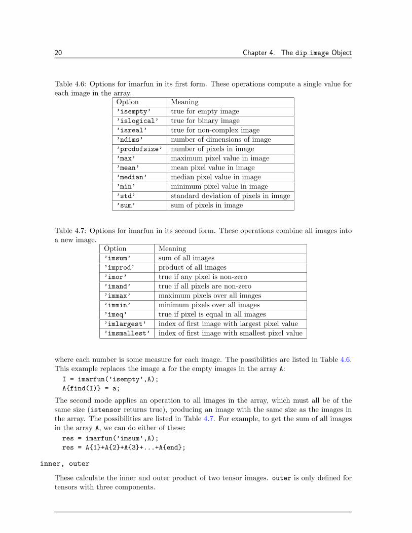
Table 4.6: Options for imarfun in its first form. These operations compute a single value foreach image in the array.
Option Meaning’isempty’ true for empty image’islogical’ true for binary image’isreal’ true for non-complex image’ndims’ number of dimensions of image’prodofsize’ number of pixels in image’max’ maximum pixel value in image’mean’ mean pixel value in image’median’ median pixel value in image’min’ minimum pixel value in image’std’ standard deviation of pixels in image’sum’ sum of pixels in image
Table 4.7: Options for imarfun in its second form. These operations combine all images intoa new image.
Option Meaning’imsum’ sum of all images’improd’ product of all images’imor’ true if any pixel is non-zero’imand’ true if all pixels are non-zero’immax’ maximum pixels over all images’immin’ minimum pixels over all images’imeq’ true if pixel is equal in all images’imlargest’ index of first image with largest pixel value’imsmallest’ index of first image with smallest pixel value
where each number is some measure for each image. The possibilities are listed in Table 4.6.This example replaces the image a for the empty images in the array A:
I = imarfun(’isempty’,A);Afind(I) = a;
The second mode applies an operation to all images in the array, which must all be of thesame size (istensor returns true), producing an image with the same size as the images inthe array. The possibilities are listed in Table 4.7. For example, to get the sum of all imagesin the array A, we can do either of these:res = imarfun(’imsum’,A);res = A1+A2+A3+...+Aend;
inner, outer
These calculate the inner and outer product of two tensor images. outer is only defined fortensors with three components.

DIPimage User Manual 21
iscolor
iscolor returns true if the input image is a tensor image and contains color space information(see Section 4.8).
istensor
istensor returns true if all images in an image array are of the same size. A tensor image istreated differently than a regular image array (see Section 4.7).
isvector
isvector returns true if the image pixels are represented by vectors, that is, the image arrayis one-dimensional and has more than one component (see Section 4.7).
iterate
iterate loops through each image in the image arrays it gets as input, and calls the functionfun with the given parameters. This is a very versatile function, and allows a combination ofimage arrays, single images and other objects as input. The only requirement is that all theimage arrays are of the same size.
For example, let A and B be N-by-M dip image array objects. Then
C = iterate(’max’,A,B);
is the same asC = newimar(N,M);for ii=1:N*M, Cii = max(Aii,Bii); end
Use the function iterate to apply filters to color images.
max, min
These functions have two different forms.
In the first form, they return the global maximum/minimum in the image and, optionally, itsposition:
[value,pos] = max(a);
It is also possible to process only a specified set of dimensions. For example, this commandreturns a 1D image (assuming a is 3D), where each pixel i contains the maximum overa(i,:,:):
value = max(a,[],[2,3]);
The second form takes two images and returns an image with the supremum of the two:
c = max(a,b);
mean, std
These return the mean intensity or standard deviation of the pixel values in an image. It ispossible to add a mask:
value = mean(a,m);

22 Chapter 4. The dip image Object
As in max, it is possible to specify a set of dimensions that are to be processed:
value = mean(a,[],[2,3]);
percentile
To complement the functions max, median and min, percentile returns the p percentile ofall pixels in the image a:
value = percentile(a,p);
Note that percentile(b,50) is exactly the same as median(b), percentile(b,0) is a sillyway of computing min(b), and percentile(b,100) is a silly way of performing max(b).
This function also allows specifying a set of dimensions that are to be processed:
value = percentile (a,p,[],[2,3]);
phase
phase is defined the same as angle, and is provided because it might be easier to rememberfor some users. It returns the angle of the complex values in an image.
pow10
This function was added just to complete MATLAB’s collection of pow2, log2, and log10.
rotate
The overloaded method rotate has nothing to with MATLAB’s rotate. Applied to a 3D-vector image, it rotates the vectors around an axis given by a second vector image or vector.
smooth
smooth(a,sigma) applies tensor smoothing to the tensor image a. sigma defaults to 1.
4.11 Review of the Differences Between a dip image and a MATLABArray
As we have seen, objects of type dip image have some differences with respect of regularMATLAB arrays. The main difference is in indexing. We start counting pixels from 0, andthe first index counts from left to right. This ordering is also used by functions such as size,in which the first number is the image width and the second one the height. Finally, ndims canreturn 0 or 1, which it never does for MATLAB arrays, and size can return an empty arrayor a scalar, which it never does for MATLAB arrays. The reason is that zero-dimensional andone-dimensional images are allowed, and are not seen as a special case of two-dimensionalimages. Furthermore, singleton dimensions at the end are not ignored.
When a MATLAB command results in an object of type dip image, and it is not ended witha semicolon, the image is displayed to a figure window, instead of having its pixel valuesshown in the command window. This is the default behavior, but can be overridden.
There are no array operators for scalar images, all operators work on a pixel-by-pixel basis.All functions that work on the columns of numeric arrays work on the image as a whole when

DIPimage User Manual 23
applied to a dip image object.
A collection of images can be stored in an object of type dip image. For the purposes ofthe toolbox, such an object is called a dip image array. Syntax for indexing into such acollection is similar to that used to index into a cell array (which is a collection of anytype of arrays), but should not be confused for one. A special type of image array is usedas a tensor image, for which a whole range of functions is available. Color images are tensorimages with color space information.
Objects of type dip image cannot be used in functions of the MathWorks’ Image ProcessingToolbox. Although most of MATLAB’s functions work on dip image objects, not everyfunction will work as expected. Use the functions double or uint8 to convert the image to aformat recognizable by these functions.

Chapter 5
The dip measurement Object
The function measure (and the low-level dip measure function in DIPlib) returns the mea-surement results in an object of type dip measurement. It contains all the measures done onan image in a manageable way.
5.1 Extracting Measurement Data
The data in the dip measurement object can be accessed in a very simple way, but only forreading, not writing (i.e. data manipulation is not allowed).
Indexing with parentheses is used to access the measurements belonging to one or moreobjects. The index used must match the label ID of the object in the image, and the returnedvalue is an object of type dip measurement.
The dot operator is used to extract the values corresponding to a single measurement. Thearray returned is of type double.
For example,
msr(11:15).size
will return a double array with five elements, being the sizes for objects number 11 through15. Note that element 11 doesn’t need to be placed 11th in the list of measurements. If onlyobjects starting at 10 were measured, the above example is equivalent to
msr.size(2:6)
since msr.size returns a double array, whose second element would be the size of objectnumber 11.
The end method will return the last label ID in the object. double converts the data in theobject to a double array, loosing the names of the measurements and the label IDs.
5.2 Other Information on the dip measurement Object
Besides extracting the measured data, you might want to gain more knowledge on the objectyou are dealing with (e.g. which measurements were taken and how many of them are there).This section describes functions used for this purpose.
fieldnames returns the names of the measurements present in the object.
isempty returns true if there is no data in the object.
size returns the number of IDs as the first dimension, and the number of measurements asthe second. Note that the number of measurements returned by size does not need to be
24

DIPimage User Manual 25
equal to the number of names returned by fieldnames. If a measurement contains morethan one value for each object, each of these is taken as a measurement. Thus, the numberof measurements is the number of scalar values assigned to each object. size(double(msr))returns the same value as size(msr).
5.3 Combining Measurement Data
To join measurements produced by different calls to measure, use the default MATLABsyntax. However, there is the limitation that, when joining measurements, they must containeither the same measurements on different objects, or different measurements on the sameobjects. Horizontal and vertical catenations produce different effects.
[A,B] joins two measurement objects with the same label IDs, but different measurements.If some measurements are repeated, or if the label IDs don’t match, an error is generated.
[A;B] joins two measurement objects with the same measurements, on different label IDs. Ifsome IDs are repeated, or if the measurements don’t match, an error is generated.
In some cases, objects in different images have the same labels. These need to be changedbefore catenation is possible. This is done by the following syntax:
msr.id = 51:73;
The length of the array assigned to the IDs must have the same number of elements as themeasurement object.
Similarly, it is possible to measure the same thing on different images of the same objects. Forexample, one might measure the average grey-value on all three channels of an RGB image.To join these measurements into a single object, it is possible to add a prefix to the names ofthe measurements:
msr1.prefix = ’red_’;msr2.prefix = ’green_’;msr3.prefix = ’blue_’;msr = [msr1,msr2,msr3];
Note that this prefix cannot be changed, only added to. For example,msr.prefix = ’A’;msr.prefix = ’B’;
causes the measurements in msr to have names like ’BAsize’.
5.4 Converting a dip measurement Object to a dataset Object
The dip measurement object provides an overloaded version of the dataset function, whichwill convert the measurement object into a PRTOOLS data set. An optional second argumentallows giving each object a class ID:
ds = dataset(msr,[1,1,1,2,2,3,2,3,3,2,1])
For more information on the PRTOOLS pattern recognition toolbox, go tohttp://www.qi.tnw.tudelft.nl/˜bob/PRTOOLS.html.

26 Chapter 5. The dip measurement Object
5.5 Creating a dip measurement Object with Your Own Data
To create an object of type dip measurement, use the dip measurement function. Its syntaxis:
msr = dip_measurement(id,’msrname1’,msr1,’msrname2’,msr2,...)
where id is a vector containing the object IDs, and ’msrname1’ and msr1 are the nameand results of a measurement. The number of columns in msr1 should match the number ofelements in id, as each of the columns represents the result of a measurement on a singleobject.
If the name of a measurement is not given, ’dataX’ is assumed, where the ‘X’ is the ordinalnumber of the measurement. If id is not given, 1:N is assumed. Note that the only way it ispossible to recognize whether id is missing is if the first argument is a string.
5.6 Backwards Compatibility
The dip measurement object is new to version 1.1 of the toolbox. However, it has beenimplemented in such a way that most old code doesn’t break. The structure that used to bereturned by measure in earlier versions can still be obtained with the struct function:
oldmsr = struct(msr);
The dip measurement constructor can be used to convert this structure back to an object.Converting to a structure is the only way of manipulating the measurement data.

Chapter 6
Figure Windows
The display is a very important part of any image-processing package. dip image objectscontaining scalar or color images with 1 to 3 dimensions are displayed to MATLAB’s figurewindows. These windows are completely cleared beforehand, meaning that images nevershare a window with each other or with other graphical elements. This chapter describes thepossible interactions with figure windows, how to link variables with them, and their placingon the desktop.
6.1 The Figure Window Menus
The display for an image contains four menus: “File”, “Sizes”, “Mappings” and “Actions”.
The first menu contains a “Save display...” option that saves the display to a TIFF file. Thisallows you, for example, to save an image with labels, or to zoom into a portion of an imageand only save that. It also contains a “Close” and a “Clear” item. On Windows machines,there is a “Copy display” option. It does the same as “Save”, but writes the image as abitmap to the clipboard, so that it can be pasted into other applications.
“Sizes” contains options that call diptruesize, which causes the image to be displayed withan aspect ratio of 1, and various different zoom factors (see Section 7.4). It also contains anoption that causes a the image to be stretched to fill the figure window. The last option onthis menu, “Default window size” resizes the window to some pre-defined size (which is 256by 256 pixels, but you can change it using dipsetpref, see Sections 7.8 and 8.4).
“Mappings” contains different ways of mapping the data for display. These options correspondto calls to dipmapping (see Section 7.3). The first section here contains stretching modes,which correspond to the range parameter in dipshow (see Section 7.2); one of these optionsis “Manual...”, which, through a dialog box, allows the user to select a custom range. Thesecond section, only available for grey-value images, selects a colormap. The options in thefirst section will sometimes change the selection of the colormap. If the image being displayedis complex, this menu allows choosing the complex to real mapping performed (magnitude,phase, real or imaginary part). For 3D images you can select the orientation of the slicesshown (X-Y, X-Z or Y-Z), as well as decide whether the stretching mode selected is to becomputed on the whole volume (“global”) or only on the current slice.
The “Actions” menu selects the actions that can be performed through the mouse. Theoptions “none”, “Pixel testing”, “Zoom”, “Looking glass” and “Pan” (which correspond tothe diptest, dipzoom, diplooking and dippan commands) are available to all image types.The 3D image display also contains an option to “Step through slices” (dipstep), and the2D grey-value-image display contains an option for “Orientation testing” (diporien). See
27

28 Chapter 6. Figure Windows
Section 6.2 for more information on these modes, and Section 7.5 for the associated commands.This menu also contains a command to enable or disable the keyboard functionality in thewindow. See Section 6.3 for more information on this.
Finally, the “Actions” menu on 3D images contains some more options:
• “Link displays” (diplink, see Section 7.6) allows the user to link a 3D display withother 3D displays. When stepping through the slices of this image, or changing theorientation of the slicing, the images in the other displays will be kept in sync. Thiscan be used to easily compare various 3D images.
• “Animate” (dipanimate) will step through all slices in sequence. Calling this functionfrom the command line allows the user to choose the speed of this animation.
• “Max projection” and “Sum projection” (dipprojection) open a new window with thechosen type of projection, along the current visualization axis.
• “Isosurface plot” (dipisosurface) also opens a new window, showing an isosurface plotof the image. This window contains some controls to modify the surface. You shouldbe aware that it takes a while to generate an isosurface. It is recommended to smoothand down-sample an image before generating an isosurface plot.
6.2 Using the Mouse in Figure Windows
As discussed above, the “Actions” menu allows selecting a mode for the mouse to workin. Depending on the dimensionality and type of the image, the modes are (the commandsbetween brackets can also be used to turn these modes on and off, see Section 7.5):
• “None”: The mouse does nothing.
• “Pixel testing” (diptest): The mouse is used to examine pixel values and location.
• “Orientation testing” (diporien): The mouse is used to examine local orientation.
• “Zoom” (dipzoom): The mouse is used to zoom the image in and out.
• “Looking glass” (diplooking): The mouse is used to enlarge a part of the image.
• “Pan” (dippan): The mouse is used to pan the image if it doesn’t fit in the window.
• “Step through slices” (dipstep): The mouse is used to step through the slices of a 3Dvolume.
When diptest is turned on, depressing the left mouse button will cause the current cursorposition to be displayed in the title bar, together with the grey-value (or color values) ofthe pixel at that location. It is possible to move the mouse while holding down the button.Depressing the right mouse button does the same thing, but the cursor position becomes theorigin of the coordinate system. This mode allows for length measurements in images.
When diporien is first turned on, a dialog box asks for the orientation image to associateto the currently displayed image. This dialog can also calculate that image for you, usingthe function structuretensor. Depressing any mouse button over the image now convertsthe cursor into a line, aligned with the local image orientation. Like in diptest, the titlebar changes to display the coordinates and local orientation. The only way of changing theorientation image associated with this display is to set “Actions” to “None”, and then enable

DIPimage User Manual 29
diporien again. Displaying a new image in this display also removes the orientation image.
When dipzoom is turned on, the mouse can be used to zoom the image in and out:
• Clicking with the left mouse button zooms the image in (with a factor 2).
• Clicking with the right one will zoom the image out (with a factor 2).
• Double-clicking any mouse button will cause the image to be stretched to fill the figurewindow.
• Dragging a rectangle around an area of interest will cause it to be zoomed-in on.
The aspect ratio is set to 1:1 when zooming in or out, except after double-clicking. SeeSection 6.3 to learn how to zoom using the keyboard.
dippan enables the user to use the mouse to pan (move) the image if it is larger than thewindow. Just press the left mouse button and move the mouse with the button down. It isalso possible to pan using the keyboard (see Section 6.3).
When dipstep is selected, it allows the user to click or drag the cursor over the image to goback and fourth through the slices that make up the 3D volume. Moving the mouse down orto the right (while holding down the left button) displays higher slice numbers. Moving themouse up or to the left displays lower slice numbers. Alternatively, click with the left mousebutton to go up, and with the right one to go down. Section 6.3 explains how to do this withthe keyboard.
6.3 Using the Keyboard in Figure Windows
When the keyboard is enabled for a display window, it can be used to step through the slicesof a 3D image, zoom in and out, and pan the image. These functions are independent of thechosen mode for the mouse under the “Actions” menu.
The keys N and P step to the next and previous slice, respectively, of a 3D image. Addition-ally, you can type the number of a slice and press Enter to go to it. Note that slice numbersstart with 0.
The keys I and O are used to zoom in and out, respectively. The zoom factor is 2. Whenzoomed in, use the following keys to pan the image and get to the area of interest: W for up,S for down, A for left, and D for right. With MATLAB 6 and newer, it is also possible touse the arrow keys.
The Esc key disables the keyboard. This is useful under Windows, where displaying an imagecauses its window to gain keyboard focus. You would have to click on the command windowto continue typing a new command. Instead, press Esc, which disables the keyboard forthe window and causes your keystrokes to be send to the command window. To enable thekeyboard again, use the menu item “Enable keyboard” under the “Actions” menu. With thecommand
dipsetpref(’EnableKeyboard’,’off’)
you disable the keyboard by default, and will have to use the above mentioned menu item toenable it. See Sections 7.8 and 8.4.
30 Chapter 6. Figure Windows
6.4 Linking Variables with Figure Windows
A variable name can be linked with the handle of a figure window, such that any imagestored in that variable will always be displayed in the same window. This is done throughthe dipfig function (see Section 7.7). It is not possible to link a single variable with morethan one figure window, but it is possible to link many variables to the same figure window.This system allows the user to create a series of figure windows that will be reused, insteadof having new windows created all the time. These links do not, however, promise that animage displayed is actually up-to-date. Changing the contents of a variable does not changethe contents of a figure window. By not adding the semicolon at the end of commands, it ispossible to automatically update the figure windows (see Section 4.2).
A special name ’other’ is defined in dipfig, that is a substitute for all variables not explicitlylinked to a figure window. It allows the user to have a window for all possible images he cancreate. ’other’ can be linked to a series of windows, which then will be used sequentially.
Closing a window does not destroy the links that were made for it. Since variable names arelinked to window handles, a window can be reopened to display the image with which it islinked.
Note that many toolbox functions that require a figure window handle as input also accept avariable name. Variable names linked with a figure window are considered aliases for a figurewindow handle.
6.5 Setting the Position of Figure Windows
The position of a figure window can be changed by manipulating its ’Position’ property,which is defined by an array with four values: left, bottom, width and height.
set(handle,’Position’,[left,bottom,width,heigth]);
The coordinates for figure windows start at the bottom-left corner of the screen, and are inscreen pixels by default. This can be changed to centimeters, inches and other units:
set(handle,’Units’,’points’);
See “MATLAB Function Reference” for more information on figure window properties.
The dipfig function has an additional optional parameter, which can be used to set theposition of a figure window at the same time that it is created. This parameter comes at theend of the parameter list, and is the same array used for the ’Position’ property:
dipfig(’a’,[400,600,256,256]);
The width and height values are those of the image that will fit in the window, and thewindow itself is drawn around this area. These values are always in screen pixels.
If an image is larger or smaller than the size of the window, the window will be resized so thatthe image fits exactly. That is, unless the ’TrueSize’ option is turned off (see Section 8.4),in which case the window will not be resized, and the image will be stretched to fit. To haveyour windows fixed on the desktop, disable the ’TrueSize’ option.
As with all other settings, the position of the figure windows cannot be saved from one sessionto the next. Add the appropriate commands to your startup.m or dipinit.m files to have

DIPimage User Manual 31
the same settings across sessions (see Section 8.3).

Chapter 7
Toolbox Functions
7.1 The GUI: dipimage
The GUI is started with the dipimage command. It contains menus with all available image-processing functions in the toolbox. After choosing any of these menu items, the GUI windowtransforms itself into a dialog box so that you can enter the appropriate parameters. Thecontrols that allow entering images have a context-menu (obtained by right-clicking in them)with the names of the images currently defined. It is possible to enter the name of a variablecontaining an image or any valid MATLAB statement that evaluates to image data. (Thesame is true for other objects, like measurements or data-sets. Also, the window selectioncontrol, which is a drop-down list, can be updated through its context-menu.) Pressing the“Execute” button causes the function to be called. There is also a button to get help on theparticular function. The whole process is rather obvious and self-explanatory, and no furtherwords shall be wasted on it.
7.2 The dipshow Function
dipshow shows a dip image object, as an image, in a figure window (that is, as long as it is abinary, grey-value or color image, and has between 1 and 3 dimensions). An optional secondargument indicates the display range required, and allows more flexibility than the optionsin the “Display” menu. The general form for dipshow is:
dipshow(a,range,colmap)
where range is either a grey-value range that should be displayed, or one of ’log’ or’base’. A range is a numeric array with two values: a lower and an upper limit. Thepixels with the same or a lower value than the lower limit will be mapped to black. Thepixels that are equal or larger than the upper limit will be mapped to white. All other valuesare linearly spaced in between. The strings ’lin’ and ’all’ and the empty array are ashortcut for [min(image),max(image)], and cause the image to be stretched linearly. Thestring ’percentile’ is a shortcut for [percentile(image,5) percentile(image,95)], and’angle’ and ’orientation’ are equivalent to [-pi,pi] and [-pi,pi]/2 respectively. Thedefault range is [0,255], which is used unless a range is given explicitly. colmap is a col-ormap. It can either be ’grey’, ’periodic’, ’labels’ or an array with 3 columns such asthose returned by the MATLAB functions hsv, cool, summer, etc. (see the help on colormapfor more information on this).
The strings ’angle’ and ’orientation’ imply ’periodic’ if no explicit colormap is given.This colormap maps both the maximum and minumum value to the same color, so as to hide
32

DIPimage User Manual 33
a jump in angle or orientation fields. The string ’labels’ implies a range of [0,255], andproduces a colormap that gives each integer value a distinct color.
The string ’log’ causes the image to be stretched logarithmically. ’base’ is a linear stretchthat fixes the value 0 to a 50% grey-value.
Examples:dipshow(a,’lin’,summer(256))dipshow(a,[0,180],’periodic’)
If the input argument is a color image, it will be converted to RGB for display.
The image is displayed in a figure window according to the name of the variable that containsthe image. Links can be made using the dipfig function (see Section 7.7). If the variablename is not registered, a new figure window is opened for the image. To overrule this behavior,it is possible to specify a figure handle in the parameter list of dipshow:
dipshow(handle,image,’lin’)
Finally, an optional argument allows you to overrule the default setting for the ’TrueSize’option. By adding the string ’truesize’ at the end of the parameter list for dipshow, you canmake sure that diptruesize is actually called. The string ’notruesize’ does the reverse.
See Chapter 6 for more information on the figure windows used by dipshow.
7.3 Figure Window Support: dipmapping
The function dipmapping can be used to change the image-to-display mapping. All menuitems under the “Mappings” menu are equivalent to a call to dipmapping. In a single com-mand, you can combine one setting for each of the four categories: range, colormap, complex-to-real mapping, the slicing direction and the global stretching for 3D images.
dipmapping(h,range,colmap,torealstr,slicingstr,globalstr)
changes the mapping settings for the image in the figure window with handle h. It is notnecessary to provide all four values, and their order is irrelevant. range can be any valueas described for dipshow in Section 7.2: a two-value numeric array or a string. colmap cancontain any of the strings described for dipshow, but not a colormap. To specify a customcolormap, use dipmapping(h,’colormap’,summer(256)). torealstr can be one of: ’abs’,’real’, ’imag’ or ’phase’. slicingstr can be one of: ’xy’, ’xz’ or ’yz’. globalstr canbe one of ’global’ or ’nonglobal’. If you don’t specify a figure handle, the current figurewill be used.
Additionally, you can specify a slice number. This is accomplished by adding two parameters:the string ’slice’, and the slice number. These must be together and in that order, butotherwise can be combined in any way with any of the other parameters. The same is truefor the m’colormap’ parameter.
7.4 Figure Window Support: diptruesize
The “Sizes” menu contains some options to call diptruesize (see Section 6.1). This functioncauses an image to be displayed with an aspect ratio of 1:1, each pixel occupying one screen

34 Chapter 7. Toolbox Functions
pixel. An argument gives the zoom factor. For example, 200 would make the image twice aslarge on the screen, but with the 1-to-1 aspect ratio:
diptruesize(200)
diptruesize(’off’) causes the image to fill the figure window, possibly loosing the aspectratio. diptruesize accepts a figure handle as an optional first argument. If you provide ahandle, you must also provide a zoom factor.
7.5 Figure Window Support: diptest, dipzoom, et al.
As explained in Section 6.1, the first section of items under the “Actions” menu correspond tothe diptest, diporien, dipzoom, diplooking, dippan and dipstep commands. We explainhere how to use the functions. The modes they activate are described in the section previouslyreferred to.
All five functions have the same syntax:
diptest on
enables the mode, and
diptest off
turns it off. diptest, by itself, toggles the state. The current window is the last one activated.You can select a window either through some mouse action on that window, or by typing inthe MATLAB command window:
figure(handle)
where handle is the handle of the figure window, which should be visible on the title bar. Ifyou know this handle, you can also directly use it as a parameter to diptest:
diptest(handle)
or
diptest(handle,’on’)
7.6 Figure Window Support: diplink
diplink is the command that corresponds to the “Link displays...” menu option for 3Dimages (see Section 6.1). It is used in much the same way as the functions in Section 7.5.When turning on, it displays a dialog box that allows the user to select the windows withwhich to link. Alternatively, it is possible to specify the figure windows with which to linkthrough the command line:
diplink(’a’,’b’,’c’,’d’)
or
diplink(1,[2,10,6])

DIPimage User Manual 35
7.7 Creating, Linking and Clearing Figure Windows: dipfig and dipclf
The single most important thing that can be customized in the DIPimage environment is theway that images are displayed to figure windows. It is possible to link a variable name with afigure handle, such that that variable is always displayed in that same window. If a variableis not linked to any window, a new one will be opened to display it. The command
dipfig a
opens a new figure window and links it to the variable named a. Whenever that variable (ifit contains an image) is displayed, it will be send to that window. If the window is closed, itwill be opened again to display the variable. It is possible to link more than one variable tothe same window, like in the next example (which uses the functional form):
h = dipfig(’a’)dipfig(h,’b’)
Finally, there is a special variable name, ’other’, that creates a link for all variables notexplicitly linked to a window. It is possible to have many windows linked to this specialname, and they will be used alternately. Creating a window for ’other’ avoids the openingof new windows for ‘unregistered’ variables.
To remove the links, type
dipfig -unlink
Unlinking only a specific variable is not implemented.
To clear all figure windows (for example at the beginning of a demo), use the function dipclf.It doesn’t change the position or size of any window, but removes the images in them. dipclfcan also be used to clear selected windows by giving it an array with handles or a cell arraywith names as an argument (in a cell array you can actually combine numeric handles andvariable names).
7.8 Toolbox Preferences: dipsetpref and dipgetpref
All toolbox preferences are stored in memory, and are only accessible through the dipsetprefand dipgetpref functions. They are listed in Section 8.4.
v = dipgetpref(’name’);
retrieves the value of the named preference. Two special forms print all current preferencesand all factory settings to the command window:
dipgetprefdipgetpref factory
Setting a preference is similar:
dipsetpref(’name’,value)
Furthermore, it is possible to set many preferences at once:
dipsetpref(’name1’,value1,’name2’,value2,’name3’,value3,...)

36 Chapter 7. Toolbox Functions
7.9 Interactive Tools: dipcrop, dipgetcoords, et al.
These are some tools that, using an image display, allow the user to select points or regionsin an image. dipgetcoords returns the coordinates of one or more points selected by clickingon an image. dipcrop returns a rectangular portion of an image selected by dragging arectangle. dipprofile returns a 1D image interpolated along a path selected by the useron the display. diproi returns a mask image (ROI stands for region of interest) created byselecting the vertices of a polygon; it can only be used with 2D images.
dipgetimage retrieves the image from a display. Use it if you lost an image but can still seeit in its display.
7.10 Image Processing Functions
The largest part of the toolbox is made out of the image processing functions. Most of themare listed in the menu system of the GUI, and all are listed by typing
help dipimage
The usage of each function can be retrieved through the help command or through the GUI.
7.11 Adding Functions to the GUI
To add a function to the GUI, it must:
• respond in certain ways to certain inputs, so that the GUI can query it for parameters,and
• be on both the MATLAB path and the DIPimage path.
The second requirement is the easiest. If you have your functions in a directory called/myhome/mytools/, then these two commands accomplish it:
addpath(’/myhome/mytools’)dipsetpref(’CommandFilePath’,’/myhome/mytools’)
The first requirement is a bit more complicated. To add this functionality to your ownfunction, copy the code in Figure 7.1. It shows a complete skeleton for a function. The linethat is not written-out is the one that assigns a structure into paramlist. This structure isthe most complicated part of the function (Figure 7.2 shows an example), but allows boththe automatic parsing of the input parameters and the drawing of the dialog box in the GUI.Automatic parameter parsing is discussed in Section 7.12.
The parameter structure paramlist contains four values:
menu Name of the menu to place the function in (string).display Name for the function in the menu (string).inparams Structure array with input parameters.outparams Structure array with output parameters.
The function will be added to the end of the menu specified (in alphabetical order). If youwant to change the order of the menu items, you will need to create a localdipmenu function(see Section 8.2).

DIPimage User Manual 37
function out = func_name(varargin)% The next line defines the parameters your function requiresparamlist = struct(...);% The next section causes this function to be integrated in% the menu systemif nargin == 1
s = varargin1;if ischar(s) & strcmp(s,’DIP_GetParamList’)
out = paramlist;return
endend% Below, add your own codeout = process_image(varargin);
Figure 7.1: Skeleton GUI function.
paramlist.inparams defines the input parameters, and contains the following fields for eachparameter:
name Variable’s name (string). Not used (for now).description Description to show the user (string).type Expected data type (string).dim check Required dimensionality.range check Expected range.required 1 or 0, to specify whether the default value is useful.default Default value to use if the parameter is not given.
paramlist.outparams defines the output parameters, and contains the following fields foreach parameter:
name Variable’s name (string). Not used (for now).description Description to show the user (string).type Data type (string).
The parameter description depends on the parameter type. What each of dim check,range check and default mean depends on the type. Also, each parameter type producesdifferent controls in the GUI. Recognized types are listed below. Please examine any of thefunctions in the toolbox that put themselves on the menu to learn more about this structure.
’image’
An object of type dip image. Other numeric arrays are converted to dip image. The GUIpresents an edit box where you can type any expression. Furthermore, a right-click in thisedit box brings up a list with variables of class dip image defined in the base workspace.
default is a string to be evaluated in the base workspace (therefore, you can use any expres-sion with names of variables in the base workspace). Typically you would use ’a’ or ’b’ as a

38 Chapter 7. Toolbox Functions
inparams = struct(...’name’,’image_in’,’percentile’,’filterSize’,’filterShape’,...’description’,’Input image’,’Percentile’,’Size of filter’,...
’Shape of filter’,...’type’,’image’,’array’,’array’,’option’,...’dim_check’,[],0,1,0,...’range_check’,[],[0,100],’N+’,’rectangular’, ’elliptic’,...
’diamond’,’parabolic’,...’required’,1,0,0,0,...’default’,’ans’,50,7,’elliptic’...
);outparams = struct(...
’name’,’image_out’,...’description’,’Output image’,...’type’,’image’...
);paramlist = struct(...
’menu’,’Filters’,...’display’,’Percentile Filter’,...’inparams’,inparams,...’outparams’,outparams...
);
Figure 7.2: Sample parameter structure (belongs to the function percf).
default value, and set required to 1. This way, the GUI shows the name of a variable possi-bly containing an image, but at the command-line (assuming you use automatic parsing) thisdefault value is never used. It is also possible to specify something like [1,1,1;1,1,1;1,1,1]as a default image (as does the function convolve).
dim check and range check are ignored. Set them to empty arrays, for in the future thesemight be used to specify the type of image required.
’measurement’
An object of type dip measurement. The same comments are valid as for ’image’.
’dataset’
An object of type dataset (from PRTOOLS). The same comments are valid as for ’image’.
’array’
A scalar value or 1D array (for 2D arrays use an image). This is probably the most complicatedtype.

DIPimage User Manual 39
dim check is an integer that can be either positive, negative or 0. If it is 0, a scalar value isexpected. If it is negative, any one-dimensional array is valid, and will be passed unchanged.Finally, if it is positive, it points to a parameter of type ’image’, whose dimensionalitydetermines the size for this array. For example, if dim ckeck is 1, and parameter 1 is a 2Dimage, then this parameter is expected to have two elements (one for each dimension). Ascalar will also be accepted (and extended by the automatic parameter parsing algorithm),but a 3-element array will not. The reason for this is that DIPlib expects some arrays to haveone value per dimension in the input image.
range check determines the valid range for the values in the array. It must be either anarray with two values (minimum and maximum valid values), an empty array (meaning[-Inf Inf]), or one of a few strings that are defined for common ranges:
• Integer types: ’N+’ = [1 Inf]. ’N-’ = [-Inf -1]. ’N’ = [0 Inf], ’Z’ = [].
• Real types: ’R’ = []. ’R+’ = [0 Inf]. ’R-’ = [-Inf 0].
Note that if you specify a range by two values, it is considered real. If you require some(finite) integer range, use the type ’option’.
default is any array that satisfies the requirements of dim check and range check. Forpositive dim check, provide a scalar as default value, since it is always valid.
’measureid’
A measurement ID in a dip measurement object.
dim check is used as in ’array’, except that it must be a positive integer. That is, it alwayspoints to a parameter of tye ’measurement’ from which to get a measurement ID.
required should be 0, and dim check and default are ignored. The default is always thefirst measurement in the dip measurement object (passing the empty string yields the defaultas well).
’option’
A value (numerical or string) selected from a list. The GUI presents a drop-down list withoptions to choose from.
range check is a cell array with possible options, for example:
• 1,2,3,4• ’rectangular’,’elliptic’,’parabolic’
required should be 0. default is any one value from the list. dim check is ignored.
’optionarray’
A cell array (with numbers or strings) selected from a list. The GUI presents an edit boxwith a button. Pressing the button brings up a dialog box that allows selecting one or moreitems from a list.
range check is as in ’option’. required should be 0. default is a cell array with valuesfrom the list, or a single value. dim check is ignored.

40 Chapter 7. Toolbox Functions
’infile’
The name of an existing file (for input). The GUI presents an edit box and a button that,when pressed, presents an “Open as...” dialog box.
range check is a string containing the mask for the filename, dim check is ignored, anddefault is a string with the default file name.
’outfile’
The name of a file (for output). The GUI presents an edit box and a button that, whenpressed, presents an “Save as...” dialog box. See the comments for ’infile’.
’indir’
The GUI presents an edit box and a button that, when pressed, presents an “Select a directory...” dialog box. range check and dim check are ignored, default gives the default directory.
’handle’
The handle of a figure window. Only figure windows created by dipshow are considered. It ispossible to enter a handle or the name of a variable (the figure to which it is linked is used).The GUI shows a drop-down list with the titles of all figure windows that fit the description.
range check is a cell array with strings that specify the type of figure window required. Allfigure windows that satisfy any of the strings are valid. Examples are:
• ’1D’,’2D’,’3D’ : either two- or three-dimensional displays.
• ’Color’,’Grey’,’Binary’ : either color, grey-value or binary displays.
• ’1D Color’,’2D Grey’ : either 1D color or 2D grey-value displays.
An empty array means that any window created by dipshow is acceptable. Note that thesestrings are not case-sensitive. It is, however, important that the order shown here is main-tained. No window will satisfy the string ’Binary 2D’, for example, but ’2D Binary’ isvalid.
dim check and default are ignored. The default value is always gcf (the current figure).
’string’
Any string. dim check and range check are ignored. default must be a string.
’boolean’
The value 1 or 0. Also accepted are the strings ’yes’, ’no’, ’true’ and ’false’, as well asonly the first character of each. The GUI presents a drop-down box with the words “yes” and“no”. The automatic parameter parsing, however, always returns either 1 or 0. dim checkand range check are ignored. default should be any of the accepted values.

DIPimage User Manual 41
% The next section handles all parameter parsingtry
[var1,var2,var3] = getparams(paramlist,varargin:);catch
if ~isempty(paramerror)error(paramerror)
elseerror(firsterr)
endend% Below, add your own codeimage_out = process_image(var1,var2,var3);
Figure 7.3: Skeleton for a function that uses automatic parameter parsing.
7.12 Automatic Parameter Parsing
To use automatic parameter parsing (through the getparams function), you no longer (sinceversion 1.4.1) need to copy files from the dipimage/private/ directory into your ownprivate/ directory. The function getparams is directly available.
The code shown in Figure 7.3 needs to be inserted into your function (after the portion usedfor the GUI functionality). As you can see, the same data structure paramlist is used forautomatic parameter parsing and for the GUI.
It is not necessary to use the function getparams. If you don’t, you will have a more flexibleparameter parsing, but if you do, you will need to write less code: parameters are guaranteedto be of the chosen types and in the chosen intervals.
Chapter 8
Customizing the DIPimage Environment
8.1 Figure Windows
The single most important thing that can be customized in the DIPimage environment is theway that images are displayed to figure windows. It is possible to link a variable name with afigure handle, such that that variable is always displayed in that same window. If a variableis not linked to any window, a new one will be opened to display it. The command dipfigis used to create these links (see Section 7.7).
8.2 Graphical user Interface
The DIPimage toolbox contains a GUI with a menu system for easy calling of toolbox func-tions. It is not necessary to use this GUI, but it is the easy way of finding the functionsdefined in the toolbox (see Section 7.1).
All functions that appear on the menus are in the toolbox directory or on the DIPimage path.If you want to add any functions to this menu system, read Section 7.11. If you want yourfunction to appear in a specific place in the menu system, you will have to create a functioncalled localdipmenus. It gives you the opportunity to edit the cell array menulist createdby dipmenus, which specifies in which menu each function should be placed. It also allowsyou to provide a list of functions not to be put on the menus at all.
The cell array menulist has two columns. The left column gives the names of the menus, theright column contains cell arrays with the function names that are to be put under each menu.Any function not mentioned in this array will be put at the bottom of the menu specified bythe function itself, in alphabetical order. See the code for dipmenus to see how it is defined.
The list of functions to be excluded overrides the menulist. Any function in this list will notbe queried when generating the menu system.
Figure 8.1 provides an example for a localdipmenus function. It adds a menu to themenulist, and puts all AVI-related functions on the exclude list. Note the string ’sep’that inserts a separator in the menu.
An alternative is to edit the dipmenus function. We do not recommend this because you willbe required to make the same changes each time you install a new version of DIPimage.
The DIPimage GUI will call the dipinit command when starting. It initializes the workingenvironment. See Section 8.3.
Another thing that can be customized in the GUI is whether the command it executes should
42

DIPimage User Manual 43
function [menulist,excludelist] = localdipmenus(menulist)I = size(menulist,1)+1;menulistI,1 = ’My Functions’;menulistI,2 = ’gaussf’,’unif’,’kuwahara’,’sep’,’closing’,’opening’;excludelist = ’readavi’,’writeavi’,’writedisplayavi’;
Figure 8.1: Sample localdipmenus function.
be printed to MATLAB’s command window. This is useful for copying and pasting thecommand being executed to some script or function. It is on by default, and can be switchedoff by typing
dipsetpref(’PutInCommandWindow’,’off’)
8.3 Initialization File
The DIPimage GUI will call the dipinit command when starting. It initializes the workingenvironment, setting up figure windows and the like. You can also call it yourself, to returnthe windows to their starting positions. You can edit this file to suit your need (or you cancreate a local copy, making sure that it sits on the MATLAB path before the original one; thisis recommended in multi-user systems). Since it is a script, not a function, it can initializesome variables if you like. It can also be used to position the DIPimage GUI to the place ofyour liking:set(0,’ShowHiddenHandles’,’on’)h = findobj(’tag’,’DIPimage_Main_Window’);set(h,’Position’,[500,600,500,100])set(0,’ShowHiddenHandles’,’off’)
8.4 Other Settings
Other settings are available through the dipsetpref command (see Section 7.8). They arelisted below:
CommandFilePath
Value: string
Default : ’’
This setting stores the path used by the DIPimage GUI to find the functions that must beadded to the menu system. The DIPimage toolbox directory does not need to be in this path,since it is always used. On UNIX and Linux systems, directories are separated by a colon(:), on Windows systems by a semicolon (;).
ComputationLimit

44 Chapter 8. Customizing the DIPimage Environment
Value: integer
Default : 65536
This only affects operations done on dip image objects in MATLAB (not operations that in-volve DIPlib itself). MATLAB can only compute using double-precision floating-point values,so images of any other type are converted to double to do the computation. This numbersets the size of the blocks in which an image is chopped to do the computation (to avoidexcessive memory usage).
CurrentImageFileDir
Value: string
Default : ’’
This setting stores the directory last visited by the file selection dialog boxes of readim,readcolorim, readroiim and writeim. It is used by these functions to open the file selectiondialog box in the directory you last used.
DebugMode
Value: ’on’ or ’off’
Default : ’off’
When this option is turned on, error messages are more verbose, and errors in the DIPimagetoolbox are easier to track. It is used for developing GUI functions.
DefaultActionState
Value: string
Default : ’diptest’
This is the action mode that will be enabled by dipshow when displaying an image to a newwindow, or to a window with a mode not compatible with the image being displayed. Possiblevalues are ’none’, ’diptest’, ’diporien’, ’dipzoom’ and ’dipstep’. See Section 6.2.
DefaultColorMap
Value: string
Default : ’grey’
This is the colormap that will be used by dipshow when displaying an image to a new window.Possible values are ’grey’, ’periodic’ and ’labels’. See Sections 7.3 and 6.1.
DefaultComplexMapping
Value: string
Default : ’abs’
This is the complex mapping mode that will be enabled by dipshow when displaying an imageto a new window, or to a window with a mode not compatible with the image being displayed.Possible values are ’abs’, ’phase’, ’real’ and ’imag’. See Sections 7.3 and 6.1.

DIPimage User Manual 45
DefaultFigureHeight
Value: integer
Default : 256
This value determines the height of a window created by dipshow or dipfig, unless a size isexplicitly given.
DefaultFigureWidth
Value: integer
Default : 256
This value determines the width of a window created by dipshow or dipfig, unless a size isexplicitly given.
DefaultGlobalStretch
Value: ’on’ or ’off’
Default : ’off’
Set this option if you want global stretching for 3D images on by default. See Sections 7.3and 6.1.
DefaultMappingMode
Value: string
Default : ’normal’
This is the mapping mode that will be enabled by dipshow when displaying an image to anew window, or to a window with a mode not compatible with the image being displayed.Possible values are ’lin’, ’percentile’, ’log’, ’base’, ’angle’ and ’orientation’. SeeSections 7.3 and 6.1.
DefaultSlicing
Value: string
Default : ’xy’
Sets the direction in which 3D volumes are sliced by default. Possible values are ’xy’, ’xz’and ’yz’. See Sections 7.3 and 6.1.
DisplayToFigure
Value: ’on’ or ’off’
Default : ’on’
When this setting is ’on’, the display method of the dip image object sends the imagedata to a figure window. When it is ’off’, disp is called instead. The display method iscalled when a MATLAB command does not end with a semicolon. See Section 4.2 for moreinformation on this behavior.

46 Chapter 8. Customizing the DIPimage Environment
EnableKeyboard
Value: ’on’ or ’off’
Default : ’on’
If you set this value to ’off’, the keyboard will be disabled when displaying an image. Thisis useful for Windows machines, on which the figure window will get keyboard focus whendisplaying an image. This can be annoying when you want to continue typing. Enable thekeyboard callback for a figure window using the appropriate menu item under “Actions”.
ImageFilePath
Value: string
Default : ’’
This setting stores the path used to find image files. The functions readim, readcolorim andreadroiim look for a file first in the current directory, and then in each of the directories givenby this option, unless the filename already contains a path. On UNIX and Linux systems,directories are separated by a colon (:), on Windows systems by a semicolon (;).
ImageSizeLimit
Value: integer
Default : 2048
This is the maximum size of an image automatically displayed through display. If any of thesizes of an image is larger, you will need to display it manually using dipshow. The reasonbehind this behavior is that such an image is most likely to be created accidentally, and notmeant for display anyway. For example, a(a>10) returns a 1D image with all pixel values ofa larger than 10; this is very useful, but not interesting to look at. For a large a (such as a3D image), the display of the resulting 1D image might require a lot of memory.
MorphologicalFlavour
Value: integer
Default : 0
This setting stores the state usually set though dip morph flavour. The value 0 causes themorphological operations to follow the definition of Serra and Soille, 2 is for the definitionfollowed by Heijmans and Haralick. Any other value is equivalent to 0.
PutInCommandWindow
Value: ’on’ or ’off’
Default : ’on’
This option causes commands that are executed from the DIPimage GUI to be printed to thecommand window. This makes it possible to copy and paste commands being executed to aMATLAB script.
TrueSize
DIPimage User Manual 47
Value: ’on’ or ’off’
Default : ’on’
This setting controls whether diptruesize is called after an image is displayed to a figurewindow (see Section 7.4).
BoundaryCondition
Value: string
Default : ’symmetric’
Setting this value causes dip setboundary to be called. This causes the algorithm thatextends the image beyond its boundary to change, for all filter operations.
Note that calling dip setboundary does change this setting, although it will not be reportedcorrectly by dipgetpref.
Truncation
Value: integer
Default : 3
Setting this value causes dip settruncation to be called. This causes all versions of theGaussian filter to change (this number represents the extent of the filtering kernel, in termsof the given parameter sigma).
Note that calling dip settruncation does change this setting, although it will not be reportedcorrectly by dipgetpref.

Chapter 9
Low-level DIPlib Interface
The DIPimage toolbox is build around DIPlib, which is a library of image-processing functionswritten in C. Most of these functions can be directly called from within MATLAB througha low-level interface. This interface is not as easy to use as the toolbox functions, but it ismore complete.
9.1 The Setup
For each function available in the low-level interface, there is a MEX-file (which is just ashared object MATLAB links to), and an M-file, which just contains some help on callingthe function. However, this help is very meager, since it only lists the name and type of eachparameter. Only when the function does more than just call the equivalent DIPlib function,are there any comments on how the function works. You will need to check the online DIPlibdocumentation to see what each of the parameters does. The online function reference canbe found at:http://www.qi.tnw.tudelft.nl/DIPlib/docs/reference/.
9.2 Calling DIPlib Functions
You will notice that the parameters required by the interface are exactly those required bythe C functions, but with some exceptions:
• The output parameters are naturally placed at the left-hand side of the function call.In the corresponding C functions, they are always on the right-hand side. The interfacegenerates an error when the C function returns an error code.
• The parameters corresponding to the random number generator are stored internallyby the interface and thus are not needed at the command line.
• The parameters corresponding to the extension of the image beyond the boundariesand the truncation of the Gaussian kernel are also not present in the interface.The default values for these parameters are used. These defaults can be set andread with the functions dip setboundary, dip getboundary, dip settruncation anddip gettruncation.
• None of the DIPlib library variables is passed back to MATLAB. This means that anyparameter of the type dip Resources and the like are not present in the MATLABinterface.
• Enumerated values in the C functions have been implemented as strings in the MATLABinterface. The function’s help will list these strings, which are easy to map to the names
48

DIPimage User Manual 49
of the enumerated values (use help parameters if in doubt). If a function requires anarray of these values, the strings should be put in a cell array.
By the way, all DIPlib interface functions have all characters in lower-case, and start withthe characters “dip ”, or “dipio ” for the functions in the dipIO extension library.
Whenever an image is required as input, it is legal to pass either a numeric MATLAB array ora dip image object. Parameters of the type dip FloatArray and the like are usually expectedto be of the same length as the dimensionality of the input image. The low-level interface isso low-level that it does not even check these simple things, and DIPlib will generate an errorif the array is not of the correct size. Many parameters are allowed to be null pointers in theC library. Sometimes it is possible to pass an empty array as such a value (for example, passan empty array as a mask image if no masking is required).
9.3 Example Function Call
As an example, let us call the DIPlib functiondip Gauss from within MATLAB. The decla-ration of the C function is:dip_Error dip_Gauss (
dip_Image in,dip_Image out,dip_BoundaryArray boundary,dip_BooleanArray process,dip_FloatArray sigmas,dip_IntegerArray parOrder,dip_float truncation
);
As explained earlier, the parameters boundary and truncation should not be used fromwithin MATLAB. The globally defined default values will be used. The parameter out shouldbe on the left of the function call. What remains is this:
out = dip_gauss(in,process,sigmas,parOrder);
which we can verify by typing
help dip_gauss
This also gives us the expected data types for each parameter. The data types correspond

50 Chapter 9. Low-level DIPlib Interface
with those expected by the C function:dip_gauss Gaussian Filter.
out = dip_gauss(in, process, sigmas, parOrder)
inImage.
processBoolean array.
sigmasReal array.
parOrderInteger array.
Parameter in can be a dip image or any numeric array. The length of the other arrays shouldmatch the dimensionality of the image. We will use a two-dimensional image a, which wewant to smooth by convolution with a Gaussian with sigma 5 in the y-direction and 2 in thex-direction. We would write
b = dip_gauss(a,[1,1],[2,5],[0,0]);
As can be read in the online help for DIPlib, parOrder indicates the order of the derivative.The process array, which is present in many DIPlib functions, can be used to apply the filteronly in some dimensions.
The dipimage/demos/ directory contains some example M-files. Examine demogdt.m for anexample on using the low-level interface.


