Chapter 7 Di/raction: Boundary Value Problems of Electromagnetic Waves 7.1 Introduction In electrostatics, a prescribed potential distribution on a closed surface uniquely determines the potential elsewhere according to the Dirichlets formulation, (r)= I S @G @n s (r 0 )dS 0 ;G =0 on S; provided G(r; r 0 ), the Greens function, is so chosen that it vanishes on the closed surface S: The normal derivative of the Greens function @G=@n can be regarded as a projection or mapping operator to convert a given distribution of the surface potential s (r 0 ) into the potential at an arbitrary observing position r: For scalar potentials, the projection operator is a scalar function, or more precisely, 1 1 matrix function. For any vector elds, too, prescribing a vector on a closed surface uniquely determines the vector led elsewhere. However, a vector eld changes its direction as well as its magnitude over a closed surface. A vector eld prescribed on a closed surface is to be converted into a vector eld with denitive direction and magnitude at the observing position. A projection operator that transforms one vector eld on a closed surface into another elsewhere must be a tensor (or dyadic) composed of appropriate eigenvectors for the vector eld of concern. For electromagnetic elds, the TE and TM eigenvectors identied in Chapter 5 can be conveniently used for this purpose. In this Chapter, a basic formulation will be developed for vector boundary value problems of electromag- netic elds, E and B: It will then be applied to some di/raction problems in which boundary electromagnetic elds are known. However, in most practical problems, it is di¢ cult to know precisely boundary elds be- cause of the feedback from the di/racted elds themselves. A rigorous analysis of di/raction problems usually requires solving integral equations based on the boundary conditions for electromagnetic waves. 7.2 Vector Greens Theorem For arbitrary vector elds E and F, by exploiting the expansion r (E r F)= r E r F E rr F; (7.1) 1
Transcript
Chapter 7
Di¤raction: Boundary ValueProblems of Electromagnetic Waves
7.1 Introduction
In electrostatics, a prescribed potential distribution on a closed surface uniquely determines the potential
elsewhere according to the Dirichlet�s formulation,
�(r) = �IS
@G
@n�s(r
0)dS0; G = 0 on S;
provided G(r; r0), the Green�s function, is so chosen that it vanishes on the closed surface S: The normal
derivative of the Green�s function @G=@n can be regarded as a projection or mapping operator to convert a
given distribution of the surface potential �s(r0) into the potential at an arbitrary observing position r: For
scalar potentials, the projection operator is a scalar function, or more precisely, 1� 1 matrix function.For any vector �elds, too, prescribing a vector on a closed surface uniquely determines the vector �led
elsewhere. However, a vector �eld changes its direction as well as its magnitude over a closed surface. A
vector �eld prescribed on a closed surface is to be converted into a vector �eld with de�nitive direction and
magnitude at the observing position. A projection operator that transforms one vector �eld on a closed
surface into another elsewhere must be a tensor (or dyadic) composed of appropriate eigenvectors for the
vector �eld of concern. For electromagnetic �elds, the TE and TM eigenvectors identi�ed in Chapter 5 can
be conveniently used for this purpose.
In this Chapter, a basic formulation will be developed for vector boundary value problems of electromag-
netic �elds, E and B: It will then be applied to some di¤raction problems in which boundary electromagnetic
�elds are known. However, in most practical problems, it is di¢ cult to know precisely boundary �elds be-
cause of the feedback from the di¤racted �elds themselves. A rigorous analysis of di¤raction problems usually
requires solving integral equations based on the boundary conditions for electromagnetic waves.
7.2 Vector Green�s Theorem
For arbitrary vector �elds E and F, by exploiting the expansion
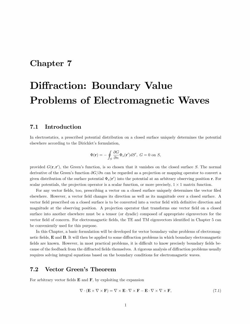
where n is the unit normal vector on the closed surface directed away from the volume V; dS = ndS: (See
Fig. 7.1.) This is a mathematical identity and holds for arbitrary vector �elds E and F.
Figure 7-1: For Es; the electric �eld speci�ed on the closed surface S; the electric �eld o¤ the surface E isuniquely determined. n is the normal unit vector directed away from the region of interest.
We now let the vector E be the electric �eld and F be one component of Green�s dyadic. In source freeregion, the electric �eld E satis�es the Helmholtz equation,
(r2 + k2)E = 0; (7.7)
and the Green�s dyadic satis�es the singular inhomogeneous Helmholtz equation
(r2 + k2)G = ��(r� r0)1; (7.8)
where 1 is the unit dyadic de�ned in terms of appropriate eigenvectors for the electromagnetic �elds. Then,
2
Eq. (7.4) yields an expression for the electric �eld E in terms of the electric �eld speci�ed on the closed
surface S;
E(r) = �IS
[(n �E)r �G+ (n�r�E) �G+ (n�E) � (r�G)] dS; (7.9)
where r � E = 0 (no charges on S) has been assumed. Note that r � G is a vector and r � G is a dyadic.
For a diagonal Green�s dyadic
G = G1; (7.10)
it follows that
r �G = rG; (7.11)
(n�r�E) �G = (n�r�E)G; (7.12)
(n�E) � (r�G) = (n�E)�rG: (7.13)
Therefore, Eq. (7.9) reduces to
E(r) = �IS
[(n �E)rG+ (n�r�E)G+ (n�E)�rG] dS: (7.14)
The scalar Green�s function G satis�es
(r2 + k2)G = ��(r� r0); (7.15)
and its explicit expression in terms of spherical harmonic expansion is
G(r; r0) =1
4� jr� r0jeikjr�r0j
= ik1Xl=0
lXm=�l
(jl (kr
0)h(1)l (kr)
jl (kr)h(1)l (kr0)
)Ylm (�; �)Y
�lm
��0; �0
�;
(r > r0
r < r0
): (7.16)
As shown in Chapter 6, the solution for the vector potential that satis�es the Helmholtz equation�r2 + k2
�A = ��0J; (7.17)
can be decomposed into TE and TM modes. In the outer region r > r0; we have the following decomposition,
are orthogonal to each other for given mode numbers l and m and the Green�s dyadic is evidently diagonal.
For di¤raction by an aperture in a large, �at conducting screen, Eq. (7.14) simpli�es to
E(r) = �2Zaperture
(n�E)�rGdS: (7.24)
This formula was originally found by Smythe based on an equivalent layer of magnetic dipole (equivalent to
a sheet of magnetic current),
dm =2
i!�0n�EdS; (7.25)
which produces a vector potential
A (r) =2
i!
ZrG� (n�E)dS: (7.26)
(Recall that an oscillating magnetic dipole creates a vector potential,
A (r) = �0rG�m '�0eikr
4�rik�m;
provided kr � 1:) Corresponding electric �eld is
E(r) = � @@tA =2
Zaperture
rG� (n�E)dS
= �2Zaperture
(n�E)�rGdS:
(Explain why we can use
E(r) = � @@tA (r) ;
here instead of going through the usual procedure
1
c2@E
@t= r�B = r� (r�A);
in terms of longitudinal and transverse components of A:) The tangential component of the di¤racted
magnetic �eld in the aperture vanishes (that is, in the aperture, the tangential magnetic �eld is equal to that
4
of the incident wave which is una¤ected by the aperture) and only the tangential component of the electric
�eld contributes to di¤raction. Likewise, the normal component of the di¤racted electric �eld vanishes in
the aperture. These follow from the symmetry property of the di¤racted electric and magnetic �eld in front
of and behind the conducting plate. The di¤racted electric �eld normal to the plate is odd with respect to
the normal coordinate z,
Ez(z) = �Ez(�z); (7.27)
and so is the tangential magnetic �eld,
ez �B (z) = �ez �B (�z) ; (7.28)
but the tangential electric �eld and normal magnetic �eld are even,
ez �E (z) = ez �E (�z) ; Bz(z) = Bz(�z): (7.29)
Therefore in the aperture, the tangential component of the di¤racted magnetic �eld should vanish. On the
surface of the conducting plate away from the aperture, tangential component of di¤racted magnetic �eld
can exist with a corresponding surface current
n�H = Js; (A m�1):
Since the normal unit vector n changes sign from one side (z < 0) to other (z > 0) ; Js = n�H is even
with respect to z; Js (z = �0) = Js (z = +0) : The surface charges induced on both sides of the conductingplate are also equal since � = "0n �E is even with respect to z: We have encountered such symmetry
properties in Chapters 2 and 3 when we analyzed leakage of electric and magnetic �elds through a hole in a
superconducting plate. In both cases, e¤ective dipoles for �elds in regions z < 0 and z > 0 are opposite to
each other and perturbed electric and magnetic �elds due to the hole have such symmetry properties which
hold in general even for radiation �elds as long as the plate can be regarded as ideally conducting.
The Smythe�s formula, Eq. (7.24), may be derived purely mathematically as follows. For a �at boundary,
the normal unit vector n is constant, say n = ez. First, we noteI(n�E)�rGdS = �
Ir� (Gn�E) dS +
IGr� (n�E) dS =
IGr� (n�E) dS; (7.30)
since for a closed surface, Ir� [G (n�E)]dS = 0: (7.31)
Recalling r �E =0 and exploiting the fact that for a unidirectional vector n;
In the case of di¤raction by an aperture in a conducting plate, n�E =0 except in the aperture. Therefore,
E(r) = �2Zaperture
(n�E)�rGdS: (7.35)
This should be equal to
E(r) = �2Zconducting plate
[(n �E)rG+ i!(n�B)G] dS; (7.36)
since in the aperture where no �eld discontinuity exists, both n �E and n�B vanish. (They are odd functionsof z:)
Rigorous analysis of di¤raction by an aperture in a conducting screen is extremely di¢ cult mainly because
in Eqs. (7.14) and (7.24), the �elds on the surface and in aperture are the di¤racted �elds which are to be
found! However, in some limiting cases, sensible analytic solutions can be found. In short wavelength limit
ka� 1 where a is the size of aperture, geometric optics approximation may be used. In this case, the �eld
in the aperture may be approximated by the incident �eld. In long wavelength limit ka� 1; the �eld in the
aperture is totally unknown. However, di¤racted power can be calculated accurately using e¤ective dipoles.
Then the �eld intensity in the aperture can be estimated to be kaEi � Ei where Ei is the incident electric
�eld.
7.3 Some Examples of Aperture Di¤raction
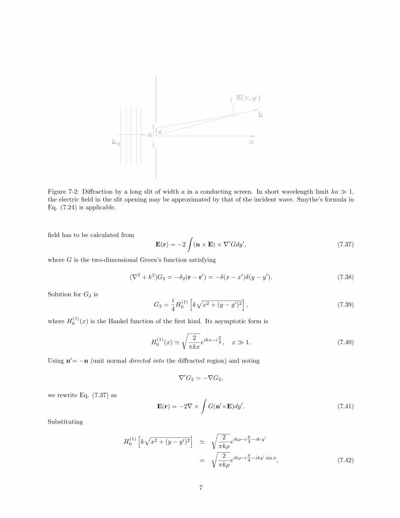
7.3.1 Long Slit
Let a plane wave be incident on a �at opaque screen having a long slit with an opening width a: The problem
is essentially two dimensional and the di¤racted wavevector k may be assumed to lie in the x � y plane.Since the slit extends from z0 = �1 to 1; we are not allowed to assume r � r0 and the di¤racted electric
6
Figure 7-2: Di¤raction by a long slit of width a in a conducting screen. In short wavelength limit ka � 1;the electric �eld in the slit opening may be approximated by that of the incident wave. Smythe�s formula inEq. (7.24) is applicable.
�eld has to be calculated from
E(r) = �2Z(n�E)�r0Gdy0; (7.37)
where G is the two-dimensional Green�s function satisfying
where H(1)0 (x) is the Hankel function of the �rst kind. Its asymptotic form is
H(1)0 (x) '
r2
�kxeikx�i
�4 ; x� 1: (7.40)
Using n0= �n (unit normal directed into the di¤racted region) and noting
r0G2 = �rG2;
we rewrite Eq. (7.37) as
E(r) = �2r�ZG(n0�E)dy0: (7.41)
Substituting
H(1)0
hkpx2 + (y � y0)2
i'
r2
�k�eik��i
�4�ik�y
0
=
r2
�k�eik��i
�4�iky
0 sin�; (7.42)
7
where
� =px2 + y2; (7.43)
and � is the angle between k and x-axis, we obtain
E(r) ' �a2k� (n0�E0)
r2
�k�eik��i
�4sin�
�; (7.44)
with � de�ned by
� =ka
2sin�: (7.45)
The function sin�=� is the familiar Fraunhofer di¤raction form factor to describe the angular (�) dependence
of the �eld intensity. The radiation (di¤racted) power per unit length of the slit is
P
l= �
Z �=2
��=2c"0 jEj2 d�: (7.46)
In short wavelength limit ka � 1; the integration limits may be approximated by from �1 to 1; and weobtain an expected result
P
l= c"0 jE0j2 a; ka� 1: (7.47)
In the opposite limit ka� 1; the electric �eld in the slit opening cannot be replaced by the incident �eld
because the current induced in the conducting plate greatly disturbs the incident �eld. The problem is dual
of scattering of electromagnetic waves by a thin, long conducting plate which will be analyzed as a separate
problem.
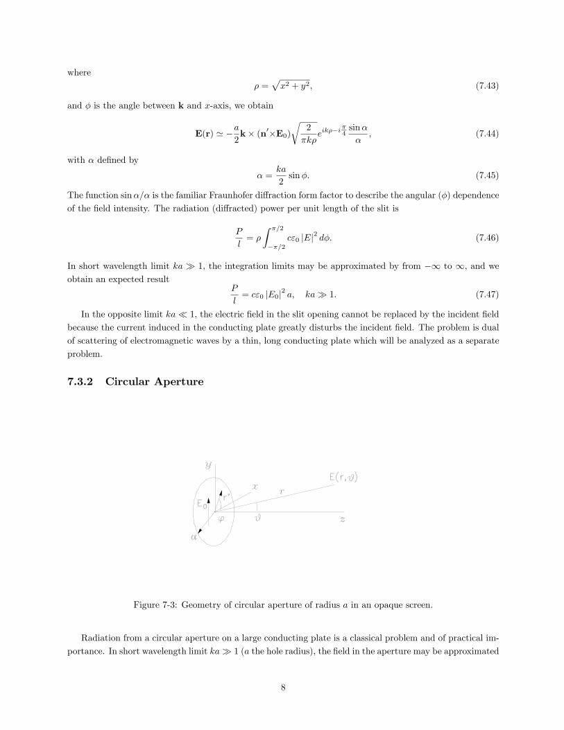
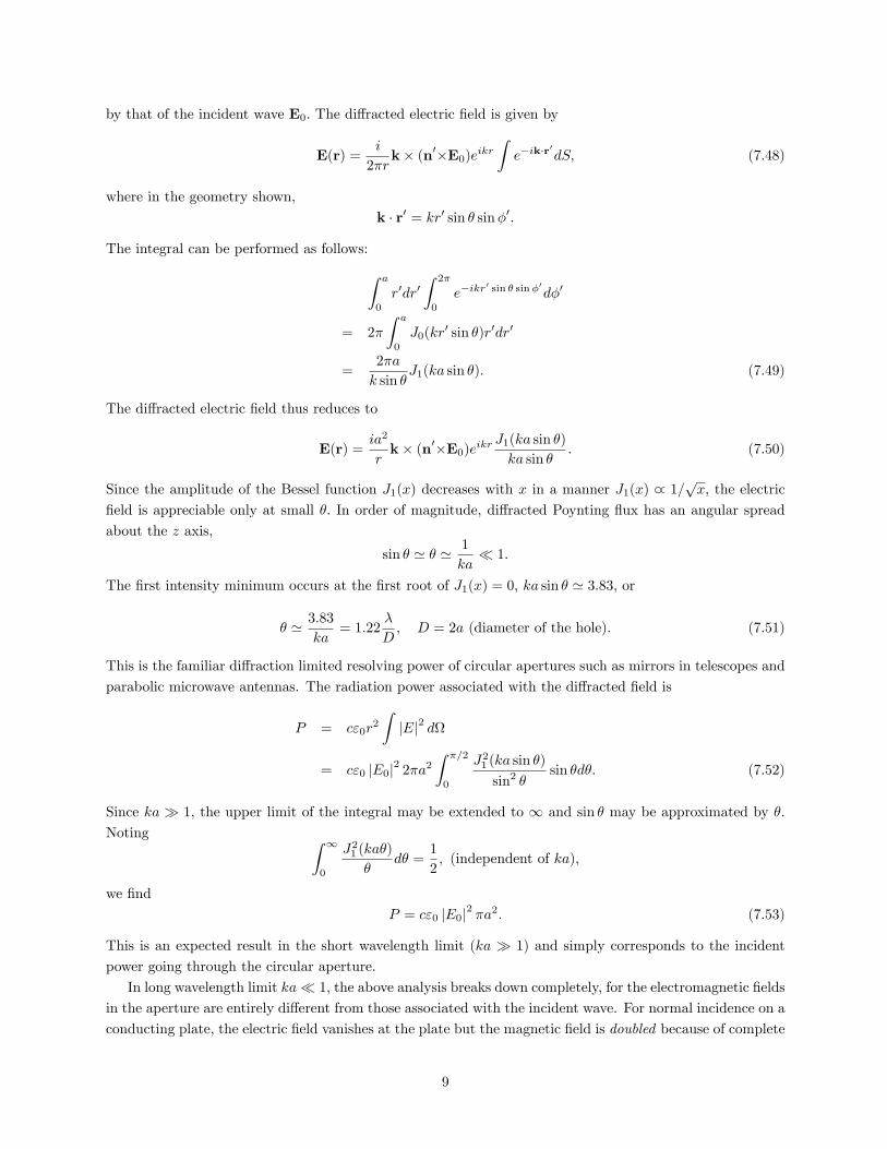
7.3.2 Circular Aperture
Figure 7-3: Geometry of circular aperture of radius a in an opaque screen.
Radiation from a circular aperture on a large conducting plate is a classical problem and of practical im-
portance. In short wavelength limit ka� 1 (a the hole radius), the �eld in the aperture may be approximated
8
by that of the incident wave E0: The di¤racted electric �eld is given by
E(r) =i
2�rk� (n0�E0)eikr
Ze�ik�r
0dS; (7.48)
where in the geometry shown,
k � r0 = kr0 sin � sin�0:
The integral can be performed as follows:Z a
0
r0dr0Z 2�
0
e�ikr0 sin � sin�0d�0
= 2�
Z a
0
J0(kr0 sin �)r0dr0
=2�a
k sin �J1(ka sin �): (7.49)
The di¤racted electric �eld thus reduces to
E(r) =ia2
rk� (n0�E0)eikr
J1(ka sin �)
ka sin �: (7.50)
Since the amplitude of the Bessel function J1(x) decreases with x in a manner J1(x) _ 1=px; the electric
�eld is appreciable only at small �: In order of magnitude, di¤racted Poynting �ux has an angular spread
about the z axis,
sin � ' � ' 1
ka� 1:
The �rst intensity minimum occurs at the �rst root of J1(x) = 0; ka sin � ' 3:83; or
� ' 3:83
ka= 1:22
�
D; D = 2a (diameter of the hole). (7.51)
This is the familiar di¤raction limited resolving power of circular apertures such as mirrors in telescopes and
parabolic microwave antennas. The radiation power associated with the di¤racted �eld is
P = c"0r2
ZjEj2 d
= c"0 jE0j2 2�a2Z �=2
0
J21 (ka sin �)
sin2 �sin �d�: (7.52)
Since ka � 1; the upper limit of the integral may be extended to 1 and sin � may be approximated by �:
Noting Z 1
0
J21 (ka�)
�d� =
1
2; (independent of ka);
we �nd
P = c"0 jE0j2 �a2: (7.53)
This is an expected result in the short wavelength limit (ka � 1) and simply corresponds to the incident
power going through the circular aperture.
In long wavelength limit ka� 1; the above analysis breaks down completely, for the electromagnetic �elds
in the aperture are entirely di¤erent from those associated with the incident wave. For normal incidence on a
conducting plate, the electric �eld vanishes at the plate but the magnetic �eld is doubled because of complete
9
re�ection. This does not mean there exists a tangential magnetic �eld of H =2H0 in the aperture because
the aperture should not a¤ect the incident magnetic �eld and the tangential component of the magnetic
�eld in the aperture is H = H0:What we can do is to �nd an e¤ective magnetic dipole moment of the hole
using 2H0 as the unperturbed �eld as we did in analyzing the leakage of magnetic �eld through a hole in a
superconducting plate. The dipole moment of the hole is
m = �8a3
3� 2H0 = �
16a3
3H0; (7.54)
which radiates at a power
P =1
2� 1
4�"0
2!4m2
3c5
=64
27�(ka)4a2Z0 jH0j2 ; (7.55)
where the factor 12 is due to radiation into half space (behind the screen). The transmission cross-section is
�t 'P
Z0 jH0j2=64
27�(ka)4a2 _ k4a6: (7.56)
The dependence � _ k4 (or !4) is the common feature of Rayleigh scattering of electromagnetic waves bysmall objects (in this case an aperture). � _ a6 indicates extremely sensitive dependence of the cross sectionon the hole radius. To order k6; the cross section is
� ' 64
27�(ka)4a2
�1 +
22
25(ka)2 + � � �
�; ka� 1: (7.57)
Since the radiation power is proportional to����Z (n�Ea)e�ik�r0dS
����2 ' E2aa4;where Ea is the electric �eld in the aperture, it is evident that the �eld is of the order of
Ea ' kaE0 � E0;
being much smaller than the incident �eld E0: This is expected since the incident wave is essentially short-
circuited at the plate and only a small �eld can leak through the aperture. The electric �eld in the aperture
has been worked out by Bouwkamp,
Ex (x; y) = i4k
3�
xypa2 � x2 � y2
E0; (7.58)
Ey (x; y) = i4k
3�
x2 + 2y2 � 2a2pa2 � x2 � y2
E0 = i4k
3�
�2 + �2 sin2 �� 2a2pa2 � �2
E0: (7.59)
Ex is an odd function of x and y and does not contribute (integrates to 0). The �eld diverges at the rim
� = a but is integrable. Integration over the aperture yieldsZ a
0
�d�
Z 2�
0
d�Ey(x; y) = �i8ka3
3E0: (7.60)
10
The di¤racted electric �eld can then be found using the Smythe�s formula which is equivalent to the �eld
due to an e¤ective magnetic dipole moment in Eq. (7.54).
Di¤raction in the regime ka ' O(1) is di¢ cult to analyze and requires numerical analysis. The trans-mission cross-section peaks at ka ' 1:56 and its value is �max ' 1:8 � �a2. This behavior is similar to thecase of scattering by a conducting sphere.
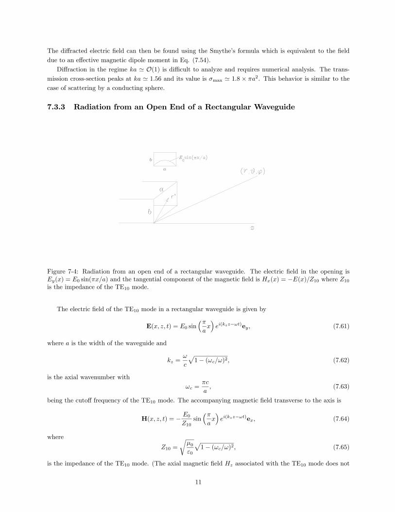
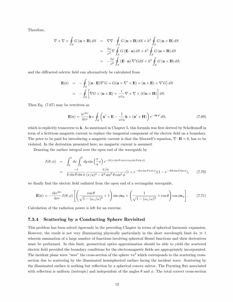
7.3.3 Radiation from an Open End of a Rectangular Waveguide
Figure 7-4: Radiation from an open end of a rectangular waveguide. The electric �eld in the opening isEy(x) = E0 sin(�x=a) and the tangential component of the magnetic �eld is Hx(x) = �E(x)=Z10 where Z10is the impedance of the TE10 mode.
The electric �eld of the TE10 mode in a rectangular waveguide is given by
E(x; z; t) = E0 sin��ax�ei(kzz�!t)ey; (7.61)
where a is the width of the waveguide and
kz =!
c
p1� (!c=!)2; (7.62)
is the axial wavenumber with
!c =�c
a; (7.63)
being the cuto¤ frequency of the TE10 mode. The accompanying magnetic �eld transverse to the axis is
H(x; z; t) = � E0Z10
sin��ax�ei(kzz�!t)ex; (7.64)
where
Z10 =
r�0"0
p1� (!c=!)2; (7.65)
is the impedance of the TE10 mode. (The axial magnetic �eld Hz associated with the TE10 mode does not
11
contribute to radiation from the aperture.) If a waveguide is truncated, the open radiates electromagnetic
waves. The Smythe�s formula is not applicable because it only pertains to radiation from apertures in a
large conducting plate. In the general di¤raction formula
E(r) = �IS
�(n �E)r0G+G(n�r0 �E) + (n�E)�r0G
�dS; (7.66)
where
G(r; r0) =eikjr�r
0j4� jr� r0j ;
we assume r � r0. Then,
G(r; r0) ' 1
4�reikr�ik�r
0;
and
r0G = �rG ' �ik 1
4�reikr�ik�r
0:
Also,
r�E = �@B@t
= i!B:
Then,
E(r) ' ieikr
4�r
IS
�k� (n0�E) + !n0�B� k(n0�E)
�e�ik�r
0dS; (7.67)
where n0= �n is the normal unit directed toward the region where the electric �eld is to be evaluated. It isnot obvious that the contribution from the second and third terms in the integrand,I
S
�!n0�B� k(n0�E)
�e�ik�r
0dS; (7.68)
is explicitly transverse (perpendicular to k) which should be the case since we are calculating radiation �eld.
To prove this, we �rst show that
r �IS
(n�B)G (r; r0) dS;
can be expressed in terms of the normal component of the electric �eld as follows.
r �IS
G (n�B) dS = �IS
r0G � (n�B) dS
=
IS
r0G � (B� n) dS
=
IS
�r0G�B
��ndS
=
IS
�r0 � (GB)
��ndS �
IS
�Gr0 �B
��ndS
= 0 +i!
c2
IS
G (E � n) dS;
where use is made of the identity IS
�r0 �A
��ndS = 0:
12
Therefore,
r�r�IS
G (n�B) dS = rr �IS
G (n�B) dS + k2IS
G (n�B) dS
=i!
c2rIS
G (E � n) dS + k2IS
G (n�B) dS
= � i!c2
IS
(E � n)r0GdS + k2IS
G (n�B) dS;
and the di¤racted eelctric �eld can alternatively be calculated from
E(r) = �IS
�(n �E)r0G+G(n�r0 �E) + (n�E)�r0G
�dS
= �IS
�rG� (n�E) + i
!"0r�r� (Gn�H)
�dS:
Then Eq. (7.67) may be rewritten as
E(r) =ieikr
4�rk�IS
�n0 �E� 1
!"0k� (n0 �H)
�e�ik�r
0dS; (7.69)
which is explicitly transverse to k: As mentioned in Chapter 5, this formula was �rst derived by Schelkuno¤ in
term of a �ctitious magnetic current to replace the tangential component of the electric �eld on a boundary.
The price to be paid for introducing a magnetic current is that the Maxwell�s equation, r �B = 0; has to beviolated. In the derivation presented here, no magnetic current is assumed.
Denoting the surface integral over the open end of the waveguide by
I(�; �) =
Z a
0
dx
Z b
0
dy sin��ax�e�ik(x sin � cos�+y sin � sin�)
=�i
k sin � sin�
�=a
(�=a)2 � k2 sin2 � cos2 �(1 + e�ika sin � cos�)(1� e�ikb sin � sin�); (7.70)
we �nally �nd the electric �eld radiated from the open end of a rectangular waveguide,
E(r) = � ikeikr
4�rI(�; �)
" cos �p
1� (!c=!)2+ 1
!sin�e� +
1p
1� (!c=!)2+ cos �
!cos�e�
#: (7.71)
Calculation of the radiation power is left for an exercise.
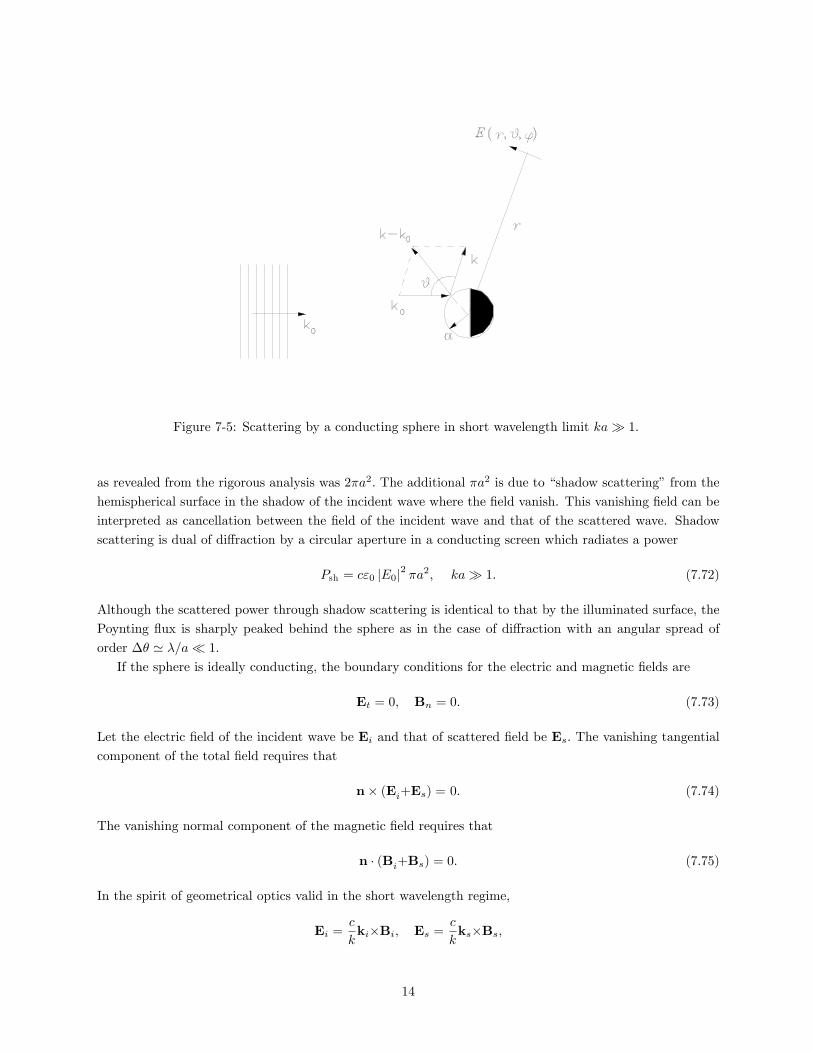
7.3.4 Scattering by a Conducting Sphere Revisited
This problem has been solved rigorously in the preceding Chapter in terms of spherical harmonic expansion.
However, the result is not very illuminating physically particularly in the short wavelength limit ka � 1
wherein summation of a large number of functions involving spherical Bessel functions and their derivatives
must be performed. In this limit, geometrical optics approximation should be able to yield the scattered
electric �eld provided the boundary conditions for the electromagnetic �elds are appropriately incorporated.
The incident plane wave �sees�the cross-section of the sphere �a2 which corresponds to the scattering cross-
section due to scattering by the illuminated hemispherical surface facing the incident wave. Scattering by
the illuminated surface is nothing but re�ection by a spherical convex mirror. The Poynting �ux associated
with re�ection is uniform (isotropic) and independent of the angles � and �. The total correct cross-section
13
Figure 7-5: Scattering by a conducting sphere in short wavelength limit ka� 1:
as revealed from the rigorous analysis was 2�a2: The additional �a2 is due to �shadow scattering�from the
hemispherical surface in the shadow of the incident wave where the �eld vanish. This vanishing �eld can be
interpreted as cancellation between the �eld of the incident wave and that of the scattered wave. Shadow
scattering is dual of di¤raction by a circular aperture in a conducting screen which radiates a power
Psh = c"0 jE0j2 �a2; ka� 1: (7.72)
Although the scattered power through shadow scattering is identical to that by the illuminated surface, the
Poynting �ux is sharply peaked behind the sphere as in the case of di¤raction with an angular spread of
order �� ' �=a� 1:
If the sphere is ideally conducting, the boundary conditions for the electric and magnetic �elds are
Et = 0; Bn = 0: (7.73)
Let the electric �eld of the incident wave be Ei and that of scattered �eld be Es: The vanishing tangential
component of the total �eld requires that
n� (Ei+Es) = 0: (7.74)
The vanishing normal component of the magnetic �eld requires that
n � (Bi+Bs) = 0: (7.75)
In the spirit of geometrical optics valid in the short wavelength regime,
Ei =c
kki�Bi; Es =
c
kks�Bs;
14
where ki is the wavevector of the incident wave and ks is that of the scattered wave. From
n� (Ei+Es) = n� (ki�Bi+ks�Bs) = 0; (7.76)
and
n� ki= n� ks; n � ki= �n � ks; (7.77)
it follows that
n� (Bi�Bs) = 0: (7.78)
Likewise, from
n� (ki�Ei�ks�Es) = 0;
we �nd
n � (Ei�Es) = 0:
With these preparations, we now apply Eq. (7.67) to the illuminated and shadow surfaces separately.
The contribution from the illuminated surface is
Eill(r) = �ieikr
4�r
Z �(k� k0)� (n0�Ei) + (k� k0)(n0�Ei)
�e�ik�r
0dS;
where the incident magnetic �eld has been eliminated through
!Bi = k0�Ei:
In the geometry shown in Fig. 7-5, the incident wave propagates in the negative z-direction,
Ei(r) = E0e�ikz0 = E0e
�ikr0 cos �0 : (7.79)
Therefore, the electric �eld di¤racted by the illuminated surface is
Eill(r) = �ieikr
4�r
Z �(k� k0)� (n0�E0) + (k� k0)(n0�E0)
�e�ikr
0 cos �0�ik�r0dS: (7.80)
Similarly, the contribution from the shadow surface is
Esh(r) = �ieikr
4�r
Z �(k+ k0)� (n0�E0)� (k� k0)(n0�E0)
�e�ikr
0 cos �0�ik�r0dS: (7.81)
The total di¤racted �eld is given by the sum of Eill and Esh : However, the angular dependence of the �eld
intensities is entirely di¤erent as explained in the introduction, namely, jEillj is insensitive to � and �; whilejEsh j sharply peaked in the direction � = � (forward scattering). Therefore, the scattered power can be
calculated separately as if the �elds were incoherent.
Noting r0 = a on the sphere surface, we �nd the phase function reduces to
kr0 cos � + k � r0 = ka�(1 + cos �) cos �0 + sin � sin �0 cos(�� �0)
�= ka f(�; �0;�; �0): (7.82)
15
By assumption ka� 1: Therefore, the exponential function
e�ikaf ; (7.83)
rapidly oscillates as �0 and �0 are varied. The slow angular dependence in the amplitude function
(k� k0)� (n0�E0) + (k� k0)(n0�E0)
can be ignored in the integration over �0 and �0 and can be taken out of the integral,
Eill(r) ' �ieikr
4�r
�(k� k0)� (n
0�Ei) + (k� k0)(n0�Ei)
��00;�
00a2Ze�ikaf(�
0;�0) sin �0d�0d�0;
where �00 and �00 indicate the angular location on the sphere surface which makes the dominant contribution
to the phase integral Ze�ikaf(�
0;�0) sin �0d�0d�0: (7.84)
Since ka� 1; major contribution to the integral comes from the angular location where the function f(�0; �0)
becomes stationary,@f
@�0=@f
@�0= 0: (7.85)
This determines
�0 =�
2; �0 = �:
This is a trivial result well expected from optical re�ection. At an observing angular location (�; �); only
the wave re�ected at (�0 = �=2; �0 = �) can be detected.
Let us Taylor expand the phase function f(�0; �0) about the stationary phase point �0 = �0 = �=2 and
�0 = �0 = �;
f(�; �0;�; �0) ' cos��
2
� 2�
��0 � �
2
�2� sin2
��
2
�(�0 � �)2 + � � �
!: (7.86)
Integration over �0 yields
Z �=2
0
exp
"ika cos
��
2
���0 � �
2
�2#sin �0d�0
' sin
��
2
�Z 1
�1exp
"ika cos
��
2
���0 � �
2
�2#d�0
= sin
��
2
� p�p
�ika cos(�=2): (7.87)
Note that the integration limits can be extended to �1 because only the region �0 ' �=2 contributes to the
16
integral. Similarly, Z 2�
0
exp
�ika cos
��
2
�sin2
��
2
�(�0 � �)2
�d�0
'Z 1
�1exp
�ika cos
��
2
�sin2
��
2
�(�0 � �)2
�d�0 (7.88)
'p�p
�ika cos(�=2) sin(�=2): (7.89)
Therefore, Ze�ikaf(�
0;�0)dS
= a2i�
ka cos(�=2)exp (�2ika cos(�=2)) : (7.90)
At the particular angular location (�=2; �); the magnitude of the vector jk� k0j is
2k cos
��
2
�; (7.91)
and the normal vector n0 is in the direction of k� k0;
n0 =
�1;�
2; �
�: (7.92)
Then,
(k� k0)� (n0�E0) + (k� k0)(n0�E0)
= 2k cos
��
2
�[n0�(n0�E0) + n0(n0�E0)]
= 2k cos
��
2
�[2n0(n0�E0)�E0] : (7.93)
The vector
2n0(n0�E0)�E0; (7.94)
has a magnitude of E0; that is,
j2n0(n0�E0)�E0j = E0;
and is perpendicular to the scattered wavevector k. (Prove this statement.) Therefore, the electric �eld
scattered (or re�ected) by the illuminated surface is
Eill(r) =a
2reikr�2ika cos(�=2) [2n0(n0�E0)�E0] : (7.95)
The amplitude jEill(r)j is independent of the angles � and � as expected from isotropic re�ection and scatteredpower can readily be found as
Pill = c"0E20r2� a2r
�2� 4�
= c"0E20 � �a2: (7.96)
17
The scattering cross-section due to scattering (essentially re�ection) by the illuminated surface is therefore
�ill = �a2: (7.97)
Scattering by the shadow surface is identical to di¤raction by a circular aperture on a conducting screen
analyzed earlier, for the boundary conditions
Ei +Es = 0; Bi +Bs = 0; (7.98)
indicate that the �elds of the incident wave can be used on the surface of the shadow hemisphere. (The
sign inversion does not a¤ect the di¤racted power.) The shape of the shadow surface is irrelevant as long as
its area projected normal to the incident wave is circular with an area �a2: To see this, let us consider the
electric �eld scattered by the shadow surface in Eq. (7.81),
Esh(r) = �ieikr
4�r
Z �(k+ k0)� (n0�E0)� (k� k0)(n0�E0)
�ei(k0�k)�r
0dS0: (7.99)
Since there is no stationary phase point in the shadow (it only occurs in the illuminated surface) and the
function ei(k0�k)�r0rapidly oscillates because of the assumption ka � 1; the integral will be nonvanishing
only if k0�k ' 0 which means predominantly forward scattering. The change in the wavevector �k = k�k0is thus perpendicular to k and k0;
�k = k sin �e�
= k sin �(cos�ex + sin�ey); (7.100)
where � is polar angle of scattered wavevector k now measured form the negative z axis, e� is the radial
unit vector in the cylindrical coordinates and � is the azimuthal angle about the z axis. The phase function
becomes
(k0 � k) � r0 = �ak sin � sin �0 cos��0 � �
�; (7.101)
and the �eld amplitude may be approximated by
(k+ k0)� (n0�E0)� (k� k0)(n0�E0) ' �2k cos �0E0; (7.102)
which is independent of � and �0. ThenZ �(k+ k0)� (n0�E0)� (k� k0)(n0�E0)
�ei(k0�k)�r
0dS0
' �2kE0a2Z �
0
sin �0d�0Z 2�
0
d�0e�iak sin � sin �0 cos(�0��) cos �0
= �2kE0Z 2�
0
d�0Z a
0
�d�e�ik� sin � cos(�0��)
= 2k� (ez �E0)Z a
0
�d�
Zd�0e�ik� sin � cos(�
0��); (7.103)
where � = a sin �0; n0 is the unit vector normal to the circular �at surface, and k � E0 ' k0 � E0 = 0 is
18
noted. The electric �eld scattered by the spherical surface in the shadow is thus given by
Esh(r) = �ieikr
2�rk� (ez �E0)
Z 2�
0
d�0Z a
0
e�ik� sin � cos(�0��)�d�: (7.104)
This is the negative of the �eld di¤racted by a circular aperture given in Eq. (7.48). Integrations over �0
and �0 yield
Esh(r) = �ia
rk� (ez �E0)
J1(ka sin �)
k sin �' � ia
rk� (ez �E0)
J1(ka�)
k�; � � 1: (7.105)
The radiation power associated with shadow di¤raction is identical to that in the case of circular aperture,
Psh = c"0E20 � �a2: (7.106)
Therefore, the total power reradiated by the sphere is
P = Pill + Psh = c"0E20 � 2�a2; (7.107)
and the total scattering cross-section in the short wavelength limit is
� = 2�a2; ka� 1: (7.108)
This is consistent with the asymptotic (ka!1) value of the general cross-section derived earlier,
�(ka) =2�
k2
1Xl=1
(2l + 1)hjAlj2 + jBlj2
i; (7.109)
where
Al = �jl(ka)
h(1)l (ka)
; Bl = �d
da[ajl(ka)]
d
da[ah
(1)l (ka)]
: (7.110)
The summation over l in Eq. (7.109) requires up to l ' O(ka) for su¢ cient accuracy and thus becomescumbersome in optical regime where ka can be huge. Also, it should be noted that the assumption of ideally
conducting sphere ("e¤ =1; �e¤ = 0) entirely breaks down in high frequency (short wavelength) regime.The e¤ective relative permittivity of ordinary metals in optical frequency regime is in general complex and
remains of the order of unity. (The relative magnetic permeability in the regime may be assumed to be
unity.)
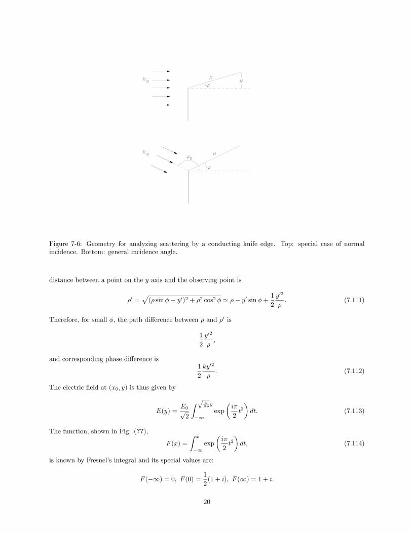
7.4 Scattering by a Knife Edge
In scattering by a knife edge, there is no geometrical scale size to speak of except for k� where � is the radial
distance from the edge tip. In short wavelength optical regime, assuming an incident electric �eld along
the plane above the edge may provide the lowest order approximation. In rigorous approach, the boundary
conditions for the electromagnetic �elds must be incorporated. We assume an observing point at (�; �): The
19
Figure 7-6: Geometry for analyzing scattering by a conducting knife edge. Top: special case of normalincidence. Bottom: general incidence angle.
distance between a point on the y axis and the observing point is
�0 =p(� sin�� y0)2 + �2 cos2 � ' �� y0 sin�+ 1
2
y02
�: (7.111)
Therefore, for small �; the path di¤erence between � and �0 is
1
2
y02
�;
and corresponding phase di¤erence is1
2
ky02
�: (7.112)
The electric �eld at (x0; y) is thus given by
E(y) =E0p2
Z qk��y
�1exp
�i�
2t2�dt: (7.113)
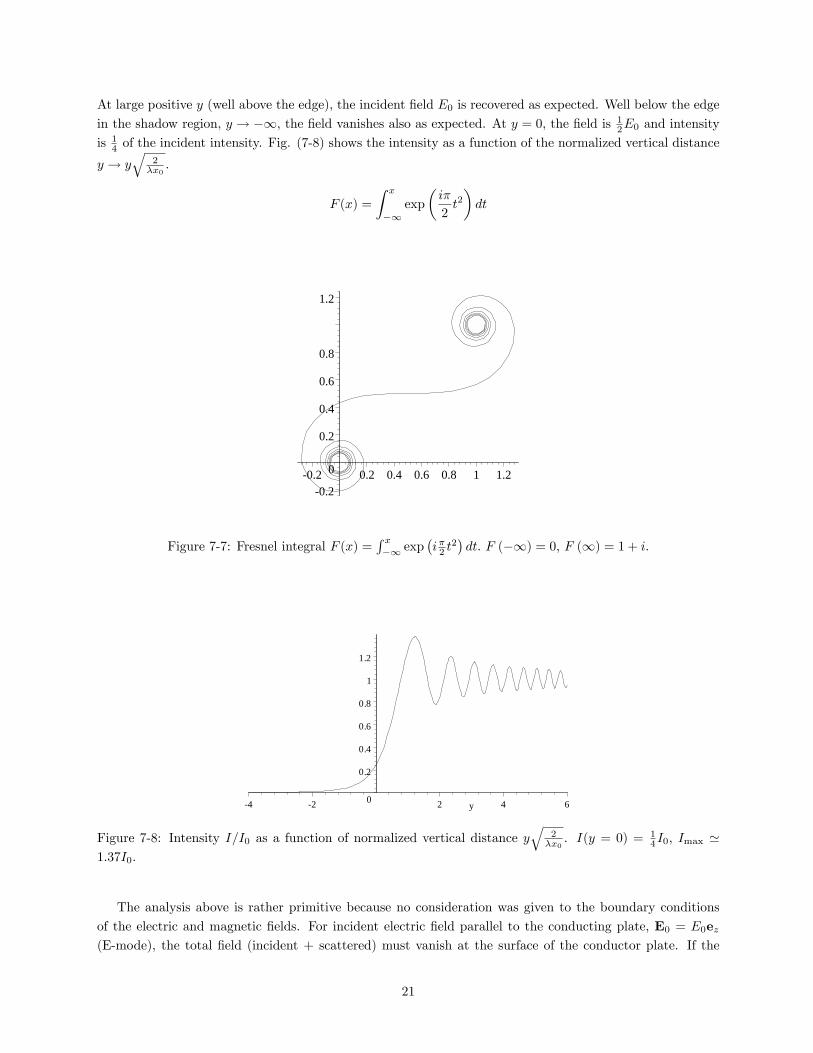
The function, shown in Fig. (??),
F (x) =
Z x
�1exp
�i�
2t2�dt; (7.114)
is known by Fresnel�s integral and its special values are:
F (�1) = 0; F (0) = 1
2(1 + i); F (1) = 1 + i:
20
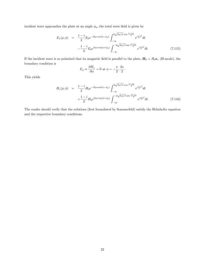
At large positive y (well above the edge); the incident �eld E0 is recovered as expected. Well below the edge
in the shadow region, y ! �1; the �eld vanishes also as expected. At y = 0; the �eld is 12E0 and intensity
is 14 of the incident intensity. Fig. (7-8) shows the intensity as a function of the normalized vertical distance
y ! yq
2�x0:
F (x) =
Z x
�1exp
�i�
2t2�dt
0.2
0
0.2
0.4
0.6
0.8
1.2
0.2 0.2 0.4 0.6 0.8 1 1.2
Figure 7-7: Fresnel integral F (x) =R x�1 exp
�i�2 t
2�dt: F (�1) = 0; F (1) = 1 + i:
0
0.2
0.4
0.6
0.8
1
1.2
4 2 2 4 6y
Figure 7-8: Intensity I=I0 as a function of normalized vertical distance yq
2�x0. I(y = 0) = 1
4I0; Imax '1:37I0:
The analysis above is rather primitive because no consideration was given to the boundary conditions
of the electric and magnetic �elds. For incident electric �eld parallel to the conducting plate, E0 = E0ez
(E-mode), the total �eld (incident + scattered) must vanish at the surface of the conductor plate. If the
21
incident wave approaches the plate at an angle �0; the total wave �eld is given by
Ez(�; �) =1� i2E0e
�ik� cos(���0)Z 2pk�=� cos
���02
�1ei
�2 t
2
dt
�1� i2E0e
ik� cos(�+�0)
Z �2pk�=� sin
�+�02
�1ei
�2 t
2
dt: (7.115)
If the incident wave is so polarized that its magnetic �eld is parallel to the plate, H0 = H0ez (H-mode), the
boundary condition is
E� _@Hz@�
= 0 at � = ��2;3�
2:
This yields
Hz(�; �) =1� i2H0e
�ik� cos(���0)Z 2pk�=� cos
���02
�1ei
�2 t
2
dt
+1� i2H0e
ik� cos(�+�0)
Z �2pk�=� sin
�+�02
�1ei
�2 t
2
dt: (7.116)
The reader should verify that the solutions (�rst formulated by Sommerfeld) satisfy the Helmholtz equation
and the respective boundary conditions.
22
Problems
7.1 An electric �eld E(�; �) = E�(�; �)e� + E�(�; �)e� is speci�ed on the surface of a sphere of radius a:
Determine the radiation electric �eld.
7.2 A magnetic �eld B(�; �) = B�(�; �)e� + B�(�; �)e� is speci�ed on the surface of a sphere of radius a:
Determine the radiation magnetic �eld.
7.3 A plane wave is incident normal to a long conducting cylinder having a square cross-section of side
a:The electric �eld is axial (Ez only) and the incident wave falls normal to one of the rectangular
surfaces. Derive an integral equation for the surface current density Jz(r): (The integral equation
can be solved numerically following the procedure developed for �nding the capacitance of a square
conducting plate.)
7.4 Repeat the preceding problem for H mode (Hz only).
7.5 A point light source is placed at a distance z0 on the axis of an opaque disk of radius a (� �): Determine
the light intensity along the axis behind the disk as a function of distance z:
7.6 A point light source is placed at a distance z0 on the axis of a circular opening of radius a in an opaque
screen. Determine the light intensity behind the disk as a function of axial distance z:
7.7 Show that in Fresnel di¤raction of incident wave normal to the plate, the maximum intensity occurs
at y ' 1:2p�x0=2 and is given by Imax ' 1:37I0 where I0 is the intensity of the incident wave.
7.8 Show that near a knife edge, an E-mode axial electric �eld
Ez(�; �) = Ap� sin
��
2
�;
and corresponding magnetic �eld
H =A
2i!�0
1p�
�cos
�
2ex + sin
�
2ey
�;
satisfy the boundary conditions. The x component of the magnetic �eld is discontinuous at � = 0
and � = 2�: Interpret this peculiarity. Show that the intensity of a wave scattered by a knife edge is
insensitive to the observing angle �: (A knife edge appears shiny regardless of observing angle.)
7.9 The transmission cross section of a small (ka� 1) circular aperture in a conducting plate is
�T =64
27�k4a6;
where a is the hole radius. Show that the magnitude of the electric �eld in the aperture should be of
the order of
Ea ' kaE0;
where E0 is the incident �eld.
Note: For incident �eld polarized in the x direction, Bouwkamp found the electric �eld component in
the aperture responsible for di¤raction,
Ey(x; y) = �8k
3�
x2 + 2y2 � 2a2pa2 � x2 � y2
E0:
23
(Ex (x; y) is an odd function of both x and y:) Integration over the aperture yieldsZEy (x; y) dS =
ZEy (r; �) rdrd� =
16
3ka3E0;
which is consistent with the e¤ective magnetic dipole,
m = �2� 83a3H0:
At the edge of a thin conductor, the electric �eld parallel to the edge vanishes in a manner Ek =p�;
while the normal component diverges as E? = 1=p� where � is the distance from the edge. For
example, the electric �eld at the rim of a charged conducting disk behaves as
E? _1q
a2 � (a� �)2=
1p2a�
:
Such properties can be exploited to �nd electric �eld when the boundary involves sharp conducting
edge.)
7.10 In low frequency limit, scatterimg by a conducting sphere may be analyzed using dipole approximation.
Relevant dipole moments are
p = 4�"0a3E0; m = �2�a3H0;
where E0 and H0 are the �elds of the incident plane wave. Show that the di¤erential scattering cross


![MODIFIED BOUNDARY INTEGRAL METHOD FOR PRESSURE …160 B.D. AGGARWALA AND P.D. ARIEL Hunt and Williams [I 5] studied the effects of a discontinuity in the electromagnetic boundary conditions](https://static.documents.pub/doc/80x56/60c03688c3acc6454f393905/modified-boundary-integral-method-for-pressure-160-bd-aggarwala-and-pd-ariel.jpg)


