Direct and Indirect Effects of Malawi’s Public Works

Program on Food Security∗

Kathleen Beegle†, Emanuela Galasso‡, and Jessica Goldberg§

April 12, 2017

Abstract

Labor-intensive public works programs are important social protection tools in low-income settings, intended to supplement the income of poor households and improvepublic infrastructure. In this evaluation of the Malawi Social Action Fund, an at-scale, government-operated program, across- and within-village randomization is usedto estimate effects on food security and use of fertilizer. There is no evidence thatthe program improves food security and suggestive evidence of negative spillovers tountreated households. These disappointing results hold even under modifications tothe design of the program to offer work during the lean rather than harvest season orincrease the frequency of payments. These findings stand in contrast to those from largePWPs in India and Ethiopia, and serves as a reminder that public works programs willnot always have significant and measurable welfare effects.

JEL Codes: I31, J22, O1. Keywords: public works, food security, Malawi.

∗These are the views of the authors and do not reflect those of the World Bank, its Executive Directors,or the countries they represent. This project was funded by the World Bank Research Committee, theKnowledge for Change program, and GLM-LIC. We thank Charles Mandala, John Ng’ambi, and the teamat the Local Development Fund in Malawi for their support of the evaluation. We thank Tavneet Suri forher inputs at the design stage of the evaluation. James Mwera and Sidney Brown provided outstandingsupervision of field activities. We thank Elizabeth Foster for her brilliant assistance with the data. Weare grateful for research assistance from Sai Luo and feedback from Jenny Aker, Arthur Alik, Alejandro dela Fuente, Pascaline Dupas, B. Kelsey Jack, Pamela Jakiela, Sebastian Galiani, Judy Hellerstein, MartinRavallion, Simone Schaner, Jeffrey Smith, and participants at PAA 2014, NEUDC 2014, IZA GLM-LIC2015, and seminars at the Inter American Development Bank, the University of Washington, the Universityof Pennsylvania, Fordham University, and Bocconi University. All errors and omissions are our own.†World Bank Ghana office. Email kbeegle@worldbank.org.‡Development Economics Research Group, World Bank, 1818 H St. NW, Washington DC 20433. Email

egalasso@worldbank.org.§3115C Tydings Hall, Department of Economics, University of Maryland, College Park MD 20742. E-mail

goldberg@econ.umd.edu.

1

1 Introduction

Labor-intensive public works programs (PWPs) are common social protection tools in low-

income settings (Grosh et al. 2008). These programs require that beneficiaries work in order

to receive a cash payment or in-kind transfer (Besley & Coate 1992). They have been

widely promoted as tools to protect poor households in the face of large macroeconomic

or agroclimatic shocks, due to their relatively rapid rollout (Ravallion 1999). They are

recently getting attention in fragile states as tools to quickly restart local economic activities

or target the employment of high risk groups (Blattman & Ralston 2015). Well-known

examples include the Employment Guarantee Scheme in Maharashtra (Ravallion, Datt &

Chaudhuri 1993), the National Rural Employment Guarantee Act (NREGA) in India (Dutta

et al. 2014), and the Productive Safety Net Project (PNSP) in Ethiopia (Hoddinott et al.

2012). Such programs are widespread – albeit not on as large a scale – in Sub-Saharan Africa,

where 39 of 48 countries have government-supported PWPs (World Bank 2015). They have

been increasingly used as a building block of national social protection portfolios.1

While many studies of cash-for-work programs focus on the potential crowding out effect of

the program on labor market outcomes or the extent of self-targeting for a given wage rate or

participation requirement (Alatas et al. 2013, Murgai, Ravallion & vandeWalle Forthcoming),

there is surprisingly limited evidence about the first order effects of the programs in increasing

consumption levels or allowing beneficiaries to smooth consumption. This paper adds to the

literature about the impact of these programs by estimating the effect of Malawi’s large-

scale PWP, which operates under the Malawi Social Action Fund (MASAF). The stated

objectives of the program are to improve food security and to increase the use of fertilizer

and other agricultural inputs. Though the PWP increased incomes by offering beneficiaries

the opportunity to earn up to US$44 in a country with a per capita gross national income of

only US$320, we find no indication that the program achieved its objectives.

Malawi’s PWP has been operational since the mid-1990s and provides short-term, labor-

intensive employment opportunities to poor, able-bodied households. The implementation

of the program is decentralized, with funding allocated to each of Malawi’s 31 districts based

on population and food security estimates carried out by the government in collaboration

with the World Food Programme (WFP). The food security objective is addressed through

a combination of support for short-term consumption as well as promotion of medium-term

food security through investments in fertilizer, which is intended to increase yields in the

subsequent season. Since 2004, the program has been designed to complement Malawi’s

1Of the 19 Sub-Saharan African countries for which the World Bank’s ASPIRE database has cost informa-tion, spending on PWPs totals more than 0.1 percent of GDP in nine and accounts for more than 10 percentof the country’s social protection budget in eight.

2

large-scale fertilizer input subsidy program by synchronizing the availability of public works

employment with the availability of fertilizer coupons, during planting season. Malawi’s

PWP ranks fourth in population covered among all such programs in low- and middle-income

countries (World Bank 2015).

We use a randomized controlled trial to evaluate the program, and to test the hypothesis

that changes to the timing of the program could increase its effect on food security, poten-

tially at the cost of investment in fertilizer. A randomized evaluation of this at-scale program

is possible because it is oversubscribed: more villages request PWP activities than can be

accommodated given the government’s budget, and, even in villages that have projects, not

all able-bodied poor households are included. The evaluation includes two levels of random-

ization: across villages and across households in treated villages. Villages that requested

PWP projects were assigned to either a pure control condition (no PWP at all) or one of

four treatment groups that offered the same wages and total number of days of employment,

but differed in the schedule of work and the frequency of payments.

Our results show that Malawi’s PWP was not effective in achieving its aim of improving

food security during the 2013 lean season. The program did not increase the use of fertilizer

or the ownership of durable goods. We do not find evidence that the program affected prices

by injecting cash into the economy. There is also no evidence of labor market tightening

induced by reduced labor supply or increased reservation wages, which implies a pure in-

come effect. The failure of the PWP to improve nutrition in either the short run (through

consumption support) or longer run (because of increased use of fertilizer) is especially trou-

bling because the MASAF PWP is the largest social protection scheme in one of the world’s

poorest countries.

The two largest PWPs (the NREGA program in India and the PNSP program in Ethiopia)

have been shown to improve some measures of household well-being. By comparison, our

findings for the Malawi PWP are very disappointing. Nonetheless, it is important to rig-

orously study program impacts even when the results are minimal or zero to avoid mis-

characterizing the potential of PWPs in developing countries on the basis of only positive

findings. The NREGA program in India had some success in stabilizing consumption (Ravi

& Engler 2015, Zimmermann 2014). NREGA, and to some extent the PSNP, differs from

Malawi’s PWP in that it functions as a true insurance program that guarantees employment

whenever households need it, for up to 100 days, rather than offering employment in a ra-

tioned fashion and only in specific time limited windows of 24 days of work in each of two

seasons.

Gilligan, Hoddinott & Taffesse (2009) find modest effects of Ethiopia’s PSNP on food

security, and Hoddinott et al. (2012) find increases in the use of fertilizer and investments

in agriculture only when combined with high levels of payments. When the program is

3

paired with an explicit strategy for improving agricultural productivity, the impacts are

larger. A more recent study of this program found significant improvements in food security

for households that participated for multiple years (Berhane et al. 2014). Relative to the

MASAF PWP, Ethiopia’s PSNP has a longer duration and higher-intensity transfers.

Not only did the Malawian program fail to improve food security for treated households,

but there is also some evidence of negative indirect effects on untreated households in villages

with the PWP, particularly in the Northern region. In contrast, social protection programs

in other settings have been found to have positive spillover effects. Imbert & Papp (2015)

and Deiniger & Liu (2013) find evidence of a general equilibrium effect of the employment

guarantee scheme in India working through an increase in the casual wage rate, with pos-

itive spillover effects for incomes of the poorest households. Angelucci & DeGiorgi (2009)

document positive spillover effects of the Oportunidades program in Mexico to households

ineligible for the program living in the same villages. Their indirect effects operate through

risk sharing; ineligible households are able to consume more through an increase in transfers

and loans from family and friends in the community. The low levels of risk sharing we detect

in our results are inconsistent with the hypothesis of a crowding-out effect of risk sharing

networks as a response to the program.

The remainder of the paper documents the details of the program, the experimental

design, and the unexpected impacts. Section 2 describes the program and the design of the

evaluation. Section 3 describes the data and outcomes of interest. In Section 4, we outline

the empirical strategy and the identification of the parameters of interest. We explain our

analytic strategy in Section 4. Then, we discuss the results on national and regional food

security in Sections 5 and 6, respectively, and for the use of fertilizer in Section 7. Section

8 discusses potential mechanisms for direct and indirect effects of the program. Section 9

concludes.

2 MASAF program and experimental design

The MASAF PWP has been operational since the mid-1990s and aims to provide short-term

labor-intensive activities to poor, able-bodied households for the purpose of enhancing their

food security, mainly through increased access to farm inputs at the time of the planting

period. The program was designed to be interlinked with Malawi’s large-scale fertilizer input

subsidy program (currently known as FISP) through the implementation of the PWP in the

planting months of the main agricultural season when the FISP distribution also occurs. The

premise behind this is that the PWP facilitates poor, credit-constrained households to access

subsidized fertilizer. This distinguishes Malawi’s program from the more traditional PWP

4

design of implementation during the lean season.

The MASAF program covers all districts of Malawi through a two-stage targeting ap-

proach. In the first stage there is pro-poor geographic targeting and in the second there is a

combination of community-based targeting and self-selection of beneficiaries. The amount of

funds given to a district is proportional to the district’s population and to the poverty rates

as well as other measures of vulnerability. District officials then target a subset of extension

planning areas (EPAs) based on poverty and vulnerability criteria. Traditional Authorities

(TAs) in the EPAs then allocate funds to a subset of selected Group Village Headmen (GVH)

who each oversee 3-10 villages. The GVH determines how many households will participate

in each village based on available funding; the GVH then works with the village committees

in each village to select participating households.

In 2012, as a response to a large currency devaluation, the program was doubled in size and

scaled up to cover about 500,000 households per year. The duration of project participation

increased from 12 days to 48 days, split in two cycles of 24 days each; the cycles were further

divided into two consecutive 12-day waves, and payments are generally made within one or

two weeks of the end of each wave. Projects were mostly road rehabilitation or construction,

with some afforestation and irrigation projects. The wage rate was 300 Malawian kwacha

(MK) per day (US$0.92/day) for a total payment of MK 3,600 for a 12-day wave (US$11.01).

Cycle 1 of the PWP is implemented during the planting season (October to December)

to align with the timing of the distribution of the Fertilizer Input Subsidy Program (FISP).

Cycle 2 of PWP was designed to take place after harvest, in June and July.

2.1 Experimental design

We use a randomized controlled trial to test variants of the PWP that are budget neutral in

terms of direct costs. Villages were stratified by geographic region to improve balance and

because geographic and cultural differences between the country’s three regions mean that

policy makers are particularly attuned to regional differences in program impacts. Villages

were randomly assigned (by computer) to one of the four treatment groups or a control

condition; households within treatment villages were randomly selected to be offered the

program.

2.1.1 Village randomization

The villages in our sampling frame were randomly assigned to one of five groups (see Figure

1). The first of these groups is a control group (Group 0) of villages that were not included

in the PWP program in the 2012-2013 Season. Groups 1 through 4 participated in the PWP

5

in the planting season (Cycle 1 of PWP). These four groups vary in terms of the timing of

the second cycle of the program and the schedule of payments in both cycles.

Among PWP-participating villages, two variants are tested:

• Timing of the program: PWP is designed to take place for two cycles of 24 days, during

planting and during post-harvest seasons. In our evaluation design, we maintain the

first cycle at the planting season, and vary the timing of Cycle 2 to take place during the

lean season (February-March) instead of during/after the harvest season (May onward).

Comparing Groups 1-2 and Groups 3-4 measures the consumption smoothing or buffer

role of PWP during the lean season.

• Schedule of payments: We introduced a variation in the payment approach from a

lump-sum payment made after 12 days of work to a split-payment variant. Under

the split-payment alternative, participants are paid three days apart, in five equal

installments of MK 720 each.2 The variation of the payment schedule was motivated

by extensive qualitative work done in preparation of the design of this project showing

that households treat the lump-sum payments of the PWP differently from income

generated through short-term casual labor (day-labor activities referred to as “ganyu”

in Malawi). Comparing Groups 1 and 3 to Groups 2 and 4 will allow us to compare

whether lump-sum payments alter the patterns of consumption and investment during

the planting or lean season.3

Payments in the study districts were facilitated by the research team for the purposes

of the evaluation. This was intended to ensure that payments were made without

delay, on specific schedules. Administrative payment records confirm that there are no

differences in time lag between work and payment across the districts.

The payment schedule may have a differential effect depending on the season. While a

lump-sum payment may facilitate investment in a lumpy input in December, split payments

may help smooth consumption during the lean season. A lump sum in February may be used

2The market price of fertilizer in Malawi at the time of this project was approximately MK 5000 for a50 kg bag. The national fertilizer subsidy program provided roughly half of households in the country withcoupons that allow two bags of fertilizer to be purchased for MK 500 each. Because households face hightransaction costs when redeeming their fertilizer coupons, including transportation costs, long wait times,and inflexibility in the days on which fertilizer can be purchased at the government shops, it is substantiallymore efficient to purchase both bags of subsidized fertilizer at once, for MK 1000 plus transportation costs(which are likely to range between MK 200 and MK 500). While MK 3600 (payment for 12 days of work)more than covers the cost of purchasing two bags of subsidized fertilizer, a single incremental payment of MK720 does not.

3Payments in the study districts were facilitated by the research team for the purposes of the evaluation,with physical delivery of the cash in conjunction with the district officials. The split-payment variant slightlyincreased the cost of implementation. E-payments, which would entail a small marginal cost of delivery, areunder consideration for future rounds of PWP.

6

for staples as well as temptation goods; divided payments can act as a form of commitment

savings that will lead to smoother consumption of staples if people otherwise have exhibit a

temptation to spend or have high discount rates even over very short periods of time.

Twenty-eight districts are included in the PWP program. For the evaluation, we ran-

domly selected 12 districts,4 stratifying by the country’s three geographic regions to ensure

that the study was representative of the country’s population and to motivate analysis of

heterogeneous effects in the three distinct regions. Within selected districts, the list of PWP-

eligible (pre-screened) villages from the District Council and Traditional Authorities was

compared with nationally representative survey data from the Integrated Household Survey

(IHS3) collected in 2010 and 2011.

The sampling frame for our analysis corresponds to the overlap between the enumeration

areas (EAs) sampled for the IHS3 and the list of communities pre-selected for PWP projects

in our 12 districts. This resulted in a total of 182 villages (EAs) to be randomly assigned

across our five treatment groups (Figure 1). For the villages selected for treatment, we

randomly chose one project in the event that the villages are mapped to two, to have unique

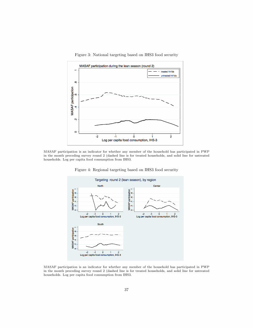
village-project pairs. The geographical targeting of the program is reflected in the regional

breakdown of the sample (see Table 1), with about one-half of the sample drawn from the

Southern region, which has a higher incidence of poverty and food insecurity (Machinjili &

Kanyanda 2012). Random assignment was stratified by region.

2.1.2 Household randomization

The second level of randomization is at the household level. This level of randomization

improves statistical power in the absence of spillovers, and provides a mechanism for testing

for the program’s indirect effects on non-participating households in the presence of spillovers.

Under the decentralized MASAF program, the GVH identifies households that are offered

PWP employment within villages selected for the program. The intention of the program is

to target poor households with able-bodied adults. As discussed below, we use the 2010/2011

IHS3 survey as a baseline for this study. By chance, then, it is likely that one or two of the

16 randomly surveyed IHS3 households in our villages will be among those chosen by the

GVH for the PWP. We term these households as “village chosen beneficiaries.”

For this study, we randomly choose 10 households from the 16 survey households in the

village to be offered the program. This strategy is analogous to studying a broad expansion of

coverage within villages selected for the program. To ensure that the experimentally induced

program offer did not affect the village selection process, the list of randomly selected house-

4The 12 districts are Blantyre, Chikwawa, Dowa, Karonga, Lilongwe, Mangochi, Mchinji, Mzimba, Nsanje,Ntchisi, Phalombe, and Zomba.

7

holds was distributed two weeks after lists of the village chosen beneficiaries were submitted

to district councils. We define these randomly chosen households as “top up” households

who are “treated” with the PWP program. Some small share of the “top up” households

will also be village chosen beneficiaries. Additionally, given the coverage rate of the status

quo program, one or two of the untreated IHS3 households were likely to be included in the

program through the village selection process.

In summary, our study has three groups of households: treated households in PWP

villages (top ups who are randomly offered the program), untreated households in PWP

villages,5 and households in non-PWP communities. By focusing on the random offer, we

estimate the intent-to-treat (ITT) effects of the program. By comparing the untreated house-

holds in PWP villages to households in non-PWP villages, we are able to measure the indirect

(spillover) effects of the program.

3 Data

The data for this study come from five rounds of panel household survey data. The basis for

the panel was the Integrated Household Survey 3 (IHS3) fielded in 2010/11 by Malawi’s Na-

tional Statistics Office. The IHS3 is a cross-section of 12,288 households in 768 communities

(16 households per community) and has extensive household and agricultural modules.

The 16 IHS3 households in our study villages were interviewed in four additional rounds:

before the public works projects started during the planting season (November 2012) after the

first cycle, pre-harvest (February 2013), after the lean season cycle, post-harvest (April-May

2013) and finally after the completion of the 2012/13 season (November 2013; see Figure 2).

In addition to the household survey data, in terms of monitoring the intervention, we have

administrative records which include the dates and amounts of payments and the identities

of recipients. These records are used to confirm that beneficiaries received payments in

accordance with the days they worked.

Our first survey (before PWP began in all but three villages) is, in effect, a second baseline

to complement the IHS3. However, it could be tainted by anticipation effects if households

in PWP villages modified their behavior before the program began in expectation of the

employment opportunities or other changes it would induce. Twenty-three communities

(approximately 13 percent of the communities in which the experiment was implemented)

were incorrectly classified as included in the IHS3, and are therefore have no IHS3 data. We

will refer to them as the “non-IHS3” sample, no true baseline data are available for this

group.6

5Including a few households selected by their village process and not through randomization.6This reflects the complexities of partnering with the Malawian government to both implement the in-

8

3.1 Food security measures

We examine food security outcomes using eight indicators and a composite measure. Our

measures include (log) per capita food expenditure7 and (log) per capita food consumption

in the last week (including home consumption). Total household calories is computed based

on the caloric value of the food consumed. A food consumption score is computed following

WFP guidelines and aims to capture both dietary diversity and food frequency; it is the

weighted sum of the number of days the household ate foods from eight food groups in the

last week.8 We include a measure of the number of food groups consumed in the last week for

seven main groups.9 We have an indicator for whether the household reported reducing meals

in the last seven days.10 A food security score is constructed according to WFP guidelines

and takes on a value of -1, -2, -3, or -4 (higher value indicates greater security).11 We report

a resilience index that is the negative of the World Food Program coping strategy index. Our

index is calculated as the negative of the weighted sum of the number of days in the past

seven days that households had to reduce the quantity and quality of food consumed; higher

values indicate greater food security.12 Finally, since many of these food security measures

are overlapping, we construct a principal components analysis index that includes all eight

measures (including the two omitted from the main tables due to space constraints) as a

composite food security measure.

tervention and collect nationally representative data. Households in these 23 communities were listed and asample of 16 households was randomly drawn during our November 2012 survey. For the IHS3 Householdsthat could not be re-interviewed, the team drew a replacement household from the original listing. About 9percent of households are replacements for the original IHS3 household.

7Omitted from the main results tables due to space constraints; available upon request.8The score is calculated based on the sum of weighted number of days in the last week the household ate

food from eight food groups: (2 * number of days of cereals, grains, maize grain/flour, millet, sorghum, flour,bread and pasta, roots, tubers, and plantains) + (3 * number of days of nuts and pulses) + (number of daysof vegetables) + (4 * number of days of meat, fish, other meat, and eggs) + (number of days of fruits) + (4 *number of days of milk products) + (0.5 * number of days of fats and oils) + (0.5 * number of days of sugar,sugar products, and honey). Spices and condiments are excluded. It has a maximum value of 126.

9The seven are described in the previous footnote, with exception of the last group (sugars).10Omitted from the main results tables due to space constraints; available upon request.11The food security score is -1 if in the past seven days, the household reports not worrying about having

enough food and reports zero days that they: (a) rely on less preferred and/or less expensive foods, (b) limitportion size at meal-times, (c) reduce number of meals eaten in a day, (d) restrict consumption by adults sothat small children may eat, or (e) borrow food, or rely on help from a friend or relative. The food securityscore is -2 if the household reports that it worried about having enough food and reports zero days for actionsa-e. The food security score is -3 if the household reports that it relied on less preferred and/or less expensivefoods and b-e are zero. The food security score is -4 if the household reports any days for b-e.

12Referring to the five actions described in the previous footnote, the resilience index is the negative of thesum of (a) + (b) + (c) + [3 * (d)] + [2 *(e)]. It has a maximum absolute value of 56.

9

4 Analysis

We analyze the ITT effect of Malawi’s PWP using household-level data from two rounds

of post-intervention surveys. Recall that our design includes two levels of randomization:

village-level randomization which varied PWP availability and payment structure, and household-

level randomization which varied the eligibility to participate within PWP villages. Our main

results pool across the four variants of the intervention to estimate the effect of any public

works opportunities in one’s village and the additional effect of being a treated household

within a PWP village. Therefore, we capture the direct effect of PWP availability on treated

households, and the indirect effect of the program on untreated households in PWP villages.

The indirect effect is important in the context of rationing.13

Using data from the lean season (survey round 2), we estimate the equation

yiv = α+ β1PWPv + β2PWPv ∗ Topupi + Γd + Θt + εiv (1)

where the indicator PWPv is a village-level indicator for the availability of any PWP program,

and Topupi is a household-level indicator that equals one if the household was randomly

selected to be offered (“treated”) the program and zero otherwise. The coefficient β1 captures

the indirect effect of the program on untreated households in PWP villages. The coefficient

on the interaction term β2 captures the marginal effect of being offered the opportunity to

participate in the program. The sum of the two coefficients β1 and β2 captures the total effect

of PWP on treated households compared with households with no PWP in their villages. All

specifications include district and week-of-interview fixed effects; standard errors are clustered

at the village level. As of survey round 2 (February 2013), all villages with PWP programs

had completed Cycle 1 (during the planting season).

In half of the PWP villages, Cycle 2 took place in the lean season, after survey round 2 and

before survey round 3. Therefore, analyses of the pre-harvest data (survey round 3) estimate

the effect of the lean season PWP compared with the standard harvest season program for

outcomes just before the harvest takes place.14 The regression specification becomes

yiv = α+δ1Leanv +δ2Leanv ∗Topupi +δ3Harvestv +δ4Harvestv ∗Topupi +Γd +Θt +εiv (2)

The sum δ1 + δ2 is the direct effect of having been offered one 24-day cycle at planting time

and a second 24-day cycle during the lean season – on outcomes just before the harvest. The

13We capture the indirect effect at the community coverage rate, slightly more than the national coveragerate of 15% since we add 10 top-up households.

14Anticipation effects due to the (announced) timing of Cycle 2 could affect survey round 2 outcomes. Inestimates available upon request, we show that the effects of the lean and harvest season variants were ofsimilar magnitude in survey round 2.

10

sum δ3 + δ4 captures the direct effect of one 24-day cycle at planting season. The difference

between the two sums is the marginal effect on household outcomes just before harvest of an

additional 24 days of potential PWP work during the lean season.

The parameters we estimate are ITT, with identification derived from randomized village

and household treatment status, rather than the endogenous participation status of house-

holds. Intent-to-treat parameters are policy relevant in that the government can control the

coverage rate and the offer of PWP activities, but not households’ decisions to take it up.

4.1 Balance

To explore the balance between treatment and control villages in terms of pre-treatment

covariates and outcomes, we use the IHS3 data from 2010/11. Although our first round of

follow-up survey pre-dates the PWP implementation in all but three villages, the survey was

conducted after the intervention was announced in treatment villages. Anticipation of the

program may have affected household behaviors.

Using the IHS3 data to examine the balance between the two groups of villages therefore

means excluding a subset of villages. So, we first examine the 23 villages that were not

included in the IHS3 national household survey in 2010/11 but were included in our sample

due to administrative errors. For this subset of villages, we do not have data prior to the

annoucement of the intervention. They were randomly assigned to our treatment/groups

(six, six, three, three, and five villages to Groups 0-4, respectively). The differences between

the IHS3 and non-IHS3 villages reflect a composition effect and have bearing on the external

validity of the results, but are orthogonal to treatment assignment. Using our first round of

follow-up data, we find that households in the non-IHS3 sample are better off than the IHS3

sample, with better educated household heads, smaller household sizes, and fewer children

below the age of 14 (see Table 2).

Unfortunately – and surprisingly, given that randomization was conducted by computer

– there is imbalance in pre-program food security at both the village and household levels

in the 159 villages for which IHS3 data are available. This is apparent in the estimates of

equation (1) for most of the food security measures from the IHS3, reported in Table 3.15

Untreated households in PWP villages had worse food security than households in control

villages according to four of six food security measures (columns 1-4, but not 5 or 6) and the

PCA index, but not the number of days of ganyu in the previous week. Treated households

fared better than their untreated neighbors by all measures, and statistically better in terms

15IHS3 surveys were conducted from March 2010 until March 2011. Balancing tests control for month andyear of survey. To control for pre-treatment levels of outcome variables in subsequent regressions given thestrong seasonality in these measures, we include the residual of each measure regressed on month and yearof survey indicators.

11

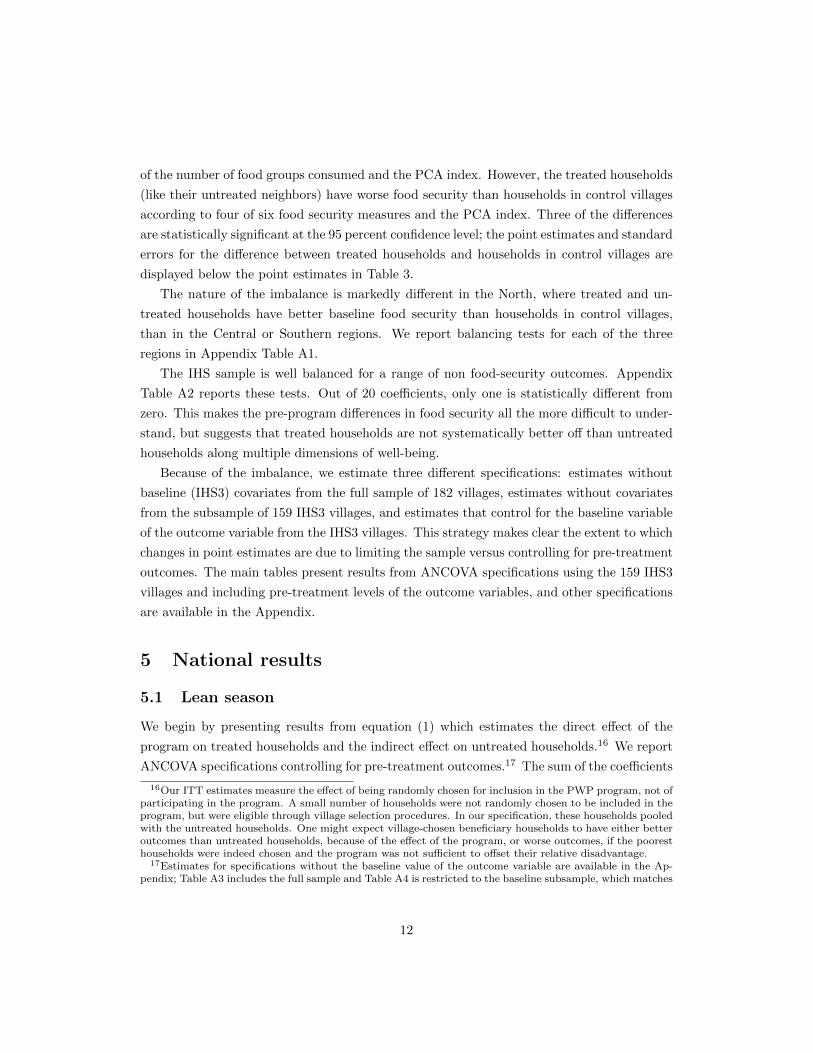
of the number of food groups consumed and the PCA index. However, the treated households

(like their untreated neighbors) have worse food security than households in control villages

according to four of six food security measures and the PCA index. Three of the differences

are statistically significant at the 95 percent confidence level; the point estimates and standard

errors for the difference between treated households and households in control villages are

displayed below the point estimates in Table 3.

The nature of the imbalance is markedly different in the North, where treated and un-

treated households have better baseline food security than households in control villages,

than in the Central or Southern regions. We report balancing tests for each of the three

regions in Appendix Table A1.

The IHS sample is well balanced for a range of non food-security outcomes. Appendix

Table A2 reports these tests. Out of 20 coefficients, only one is statistically different from

zero. This makes the pre-program differences in food security all the more difficult to under-

stand, but suggests that treated households are not systematically better off than untreated

households along multiple dimensions of well-being.

Because of the imbalance, we estimate three different specifications: estimates without

baseline (IHS3) covariates from the full sample of 182 villages, estimates without covariates

from the subsample of 159 IHS3 villages, and estimates that control for the baseline variable

of the outcome variable from the IHS3 villages. This strategy makes clear the extent to which

changes in point estimates are due to limiting the sample versus controlling for pre-treatment

outcomes. The main tables present results from ANCOVA specifications using the 159 IHS3

villages and including pre-treatment levels of the outcome variables, and other specifications

are available in the Appendix.

5 National results

5.1 Lean season

We begin by presenting results from equation (1) which estimates the direct effect of the

program on treated households and the indirect effect on untreated households.16 We report

ANCOVA specifications controlling for pre-treatment outcomes.17 The sum of the coefficients

16Our ITT estimates measure the effect of being randomly chosen for inclusion in the PWP program, not ofparticipating in the program. A small number of households were not randomly chosen to be included in theprogram, but were eligible through village selection procedures. In our specification, these households pooledwith the untreated households. One might expect village-chosen beneficiary households to have either betteroutcomes than untreated households, because of the effect of the program, or worse outcomes, if the pooresthouseholds were indeed chosen and the program was not sufficient to offset their relative disadvantage.

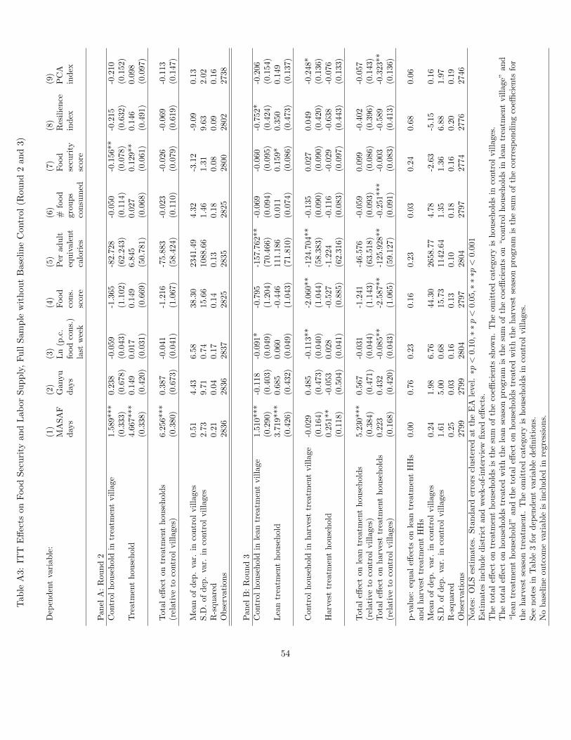
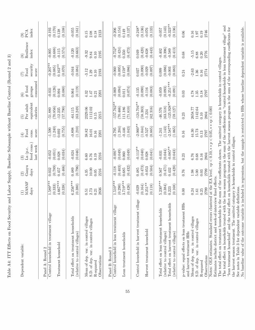
17Estimates for specifications without the baseline value of the outcome variable are available in the Ap-pendix; Table A3 includes the full sample and Table A4 is restricted to the baseline subsample, which matches

12

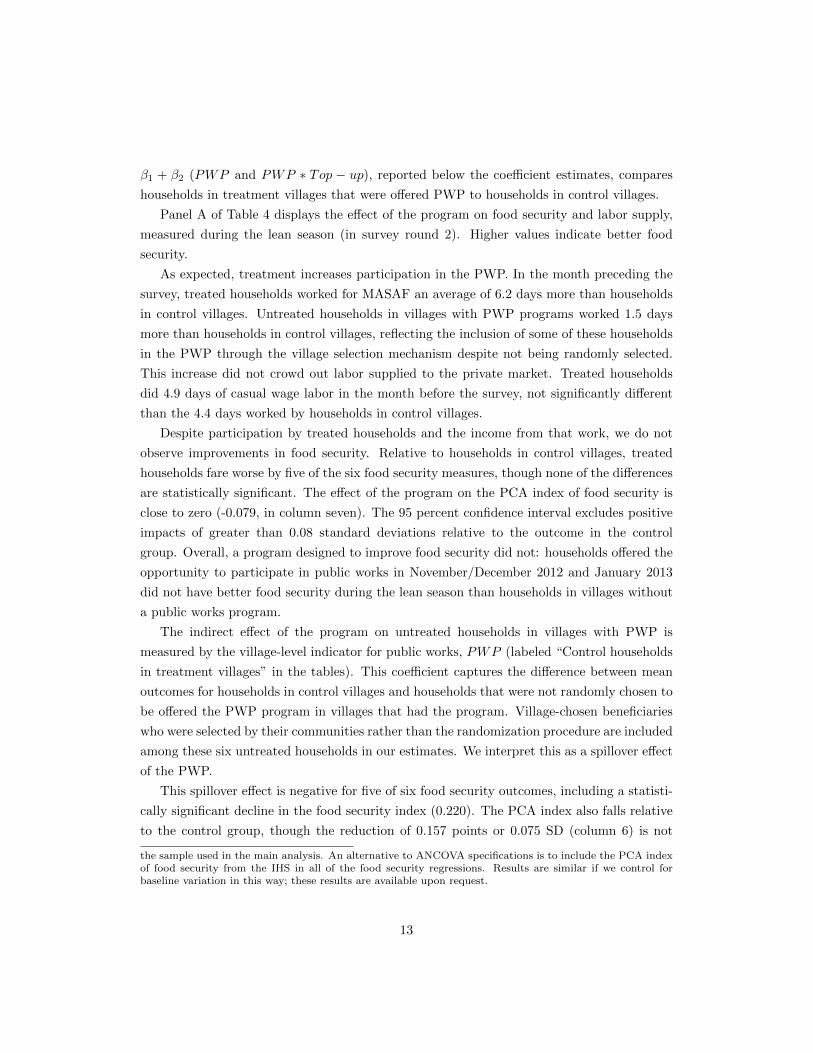
β1 + β2 (PWP and PWP ∗ Top − up), reported below the coefficient estimates, compares

households in treatment villages that were offered PWP to households in control villages.

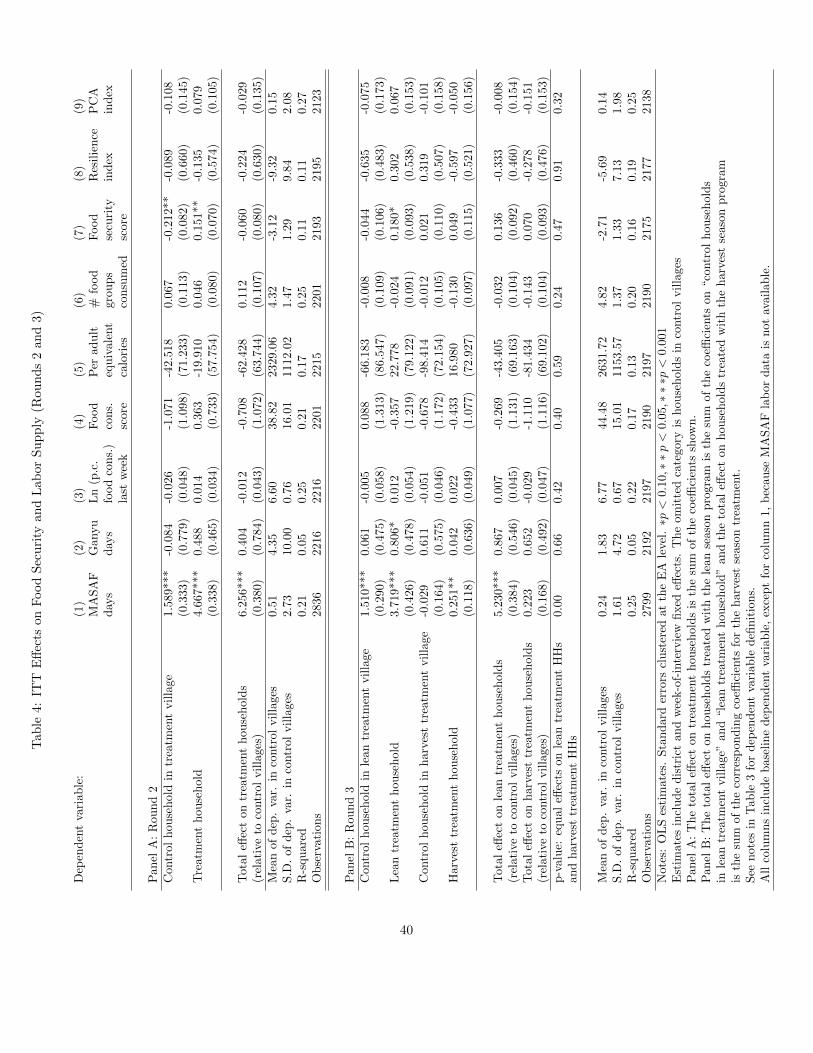
Panel A of Table 4 displays the effect of the program on food security and labor supply,

measured during the lean season (in survey round 2). Higher values indicate better food

security.

As expected, treatment increases participation in the PWP. In the month preceding the

survey, treated households worked for MASAF an average of 6.2 days more than households

in control villages. Untreated households in villages with PWP programs worked 1.5 days

more than households in control villages, reflecting the inclusion of some of these households

in the PWP through the village selection mechanism despite not being randomly selected.

This increase did not crowd out labor supplied to the private market. Treated households

did 4.9 days of casual wage labor in the month before the survey, not significantly different

than the 4.4 days worked by households in control villages.

Despite participation by treated households and the income from that work, we do not

observe improvements in food security. Relative to households in control villages, treated

households fare worse by five of the six food security measures, though none of the differences

are statistically significant. The effect of the program on the PCA index of food security is

close to zero (-0.079, in column seven). The 95 percent confidence interval excludes positive

impacts of greater than 0.08 standard deviations relative to the outcome in the control

group. Overall, a program designed to improve food security did not: households offered the

opportunity to participate in public works in November/December 2012 and January 2013

did not have better food security during the lean season than households in villages without

a public works program.

The indirect effect of the program on untreated households in villages with PWP is

measured by the village-level indicator for public works, PWP (labeled “Control households

in treatment villages” in the tables). This coefficient captures the difference between mean

outcomes for households in control villages and households that were not randomly chosen to

be offered the PWP program in villages that had the program. Village-chosen beneficiaries

who were selected by their communities rather than the randomization procedure are included

among these six untreated households in our estimates. We interpret this as a spillover effect

of the PWP.

This spillover effect is negative for five of six food security outcomes, including a statisti-

cally significant decline in the food security index (0.220). The PCA index also falls relative

to the control group, though the reduction of 0.157 points or 0.075 SD (column 6) is not

the sample used in the main analysis. An alternative to ANCOVA specifications is to include the PCA indexof food security from the IHS in all of the food security regressions. Results are similar if we control forbaseline variation in this way; these results are available upon request.

13

statistically different from zero. Not only does PWP fail to improve the food security of

households randomly offered the program, but there are also some indications that it may

reduce food security among their neighbors. 18

5.2 Pre-harvest period

As designed by the government, the second PWP cycle takes place during the harvest period,

beginning in May. This timing is suboptimal if the marginal utility of consumption is higher

and the opportunity cost of working lower during the lean season. To determine whether

changing the seasonality of the program could improve its effectiveness, our evaluation ran-

domly assigned half of the treated villages to move the second cycle, so that the public

works start sooner, in March 2013. Survey round 3 took place after the March-April Cycle

2 and just before harvest. At that time, villages assigned to the lean season treatment had

completed work cycles in November-January and March, but those assigned to the standard

harvest season treatment had not yet begun their second work cycle. The survey captures

food security and other outcomes at the end of the lean season, before the harvest has begun.

Estimating equation (2) allows us to test the marginal effect of rescheduling the second cycle

of PWP for the lean season instead of the harvest season.

We report national results in Table 4, Panel B. As in the top panel, our main results

are from ANCOVA specifications and specifications without controls are available in the

Appendix. In addition to the coefficients from equation (2), we report the total direct effect

of the lean and harvest season programs (δ1 + δ2 and δ3 + δ4, respectively) and p-values for

the tests that the direct effect of the lean season treatment equals the direct effect of the

harvest season treatment and that the corresponding indirect effects are equal.

The treatment appears to be implemented correctly: treated households in villages with

the lean season PWP report an additional 5.2 days of work for the PWP relative to households

in control villages. Treated households in villages with harvest season programs, in contrast,

do not have more PWP work in the lean season than households in the control villages. There

are no significant effects on the amount of labor supplied to casual wage labor activities, and,

reflecting the slack season, the mean number of days worked is lower than reported in the

previous round of data collection.

The direct effect of the lean season program on the food security of treated households

is small and generally not significantly different from zero. The absolute value of the effect

18Jensen & Miller (2011) offer an example of a study that attempts to improve nutrition by reducing thecost of certain foods, but finds zero or negative effects. In that paper, price subsidies for staple goods ledsome households to substitute toward more expensive calories from meat or fats; so total caloric intake fell,and nutrient intake did not rise. We do not observe an increase in dietary diversity, but note that finding anutritional elasticity close to zero is not without precedent.

14

on treated households is small for all outcomes, and there is no consistent pattern to the

direction of the effect. Similarly, spillover effects on untreated households in lean season

PWP villages are close to zero.

Households in villages assigned to the harvest season treatment (scheduled to work soon

after survey 3 was conducted) do not appear to fare as well, though effects are imprecisely

estimated. For these treated households, there are declines in five of six food security mea-

sures. The PCA index falls by 0.122 or 0.06 standard deviations, not statistically different

from zero. The spillover effect of the harvest season program is negative for four of the six

reported outcomes and the PCA index, though none of the changes are significantly different

from zero.

We cannot reject that the effect of PWP on households treated with the lean season

program equals that of households still to be treated with the harvest season PWP work

opportunities. This is despite the additional 24 days of work offered to the former group of

households. Food security for treated households in villages with lean season PWP (offered

48 days of PWP) is slightly better than households in control villages; for treated households

in harvest season PWP villages (offered 24 days as of survey round 3), food security is slightly

worse than among households in the control villages. The difference between the direct effect

of the lean season and harvest season programs on the PCA index is only 0.04 standard

deviations, and the p-value for the test that the direct effects of the two variants on the PCA

index are equal is 0.22. Differences in the indirect effects of the two program variants are

even less precisely estimated and show no consistent pattern. In short, there is little evidence

that changing the timing of Cycle 2 (the second and final 24 days of PWP) is effective in

improving food security.

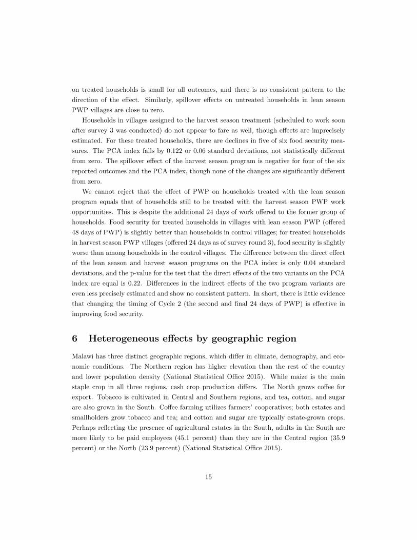
6 Heterogeneous effects by geographic region

Malawi has three distinct geographic regions, which differ in climate, demography, and eco-

nomic conditions. The Northern region has higher elevation than the rest of the country

and lower population density (National Statistical Office 2015). While maize is the main

staple crop in all three regions, cash crop production differs. The North grows coffee for

export. Tobacco is cultivated in Central and Southern regions, and tea, cotton, and sugar

are also grown in the South. Coffee farming utilizes farmers’ cooperatives; both estates and

smallholders grow tobacco and tea; and cotton and sugar are typically estate-grown crops.

Perhaps reflecting the presence of agricultural estates in the South, adults in the South are

more likely to be paid employees (45.1 percent) than they are in the Central region (35.9

percent) or the North (23.9 percent) (National Statistical Office 2015).

15

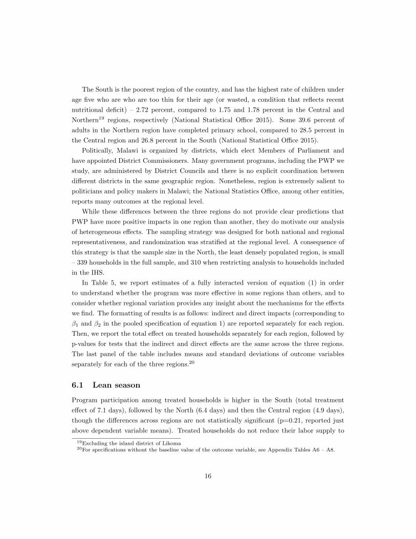
The South is the poorest region of the country, and has the highest rate of children under

age five who are who are too thin for their age (or wasted, a condition that reflects recent

nutritional deficit) – 2.72 percent, compared to 1.75 and 1.78 percent in the Central and

Northern19 regions, respectively (National Statistical Office 2015). Some 39.6 percent of

adults in the Northern region have completed primary school, compared to 28.5 percent in

the Central region and 26.8 percent in the South (National Statistical Office 2015).

Politically, Malawi is organized by districts, which elect Members of Parliament and

have appointed District Commissioners. Many government programs, including the PWP we

study, are administered by District Councils and there is no explicit coordination between

different districts in the same geographic region. Nonetheless, region is extremely salient to

politicians and policy makers in Malawi; the National Statistics Office, among other entities,

reports many outcomes at the regional level.

While these differences between the three regions do not provide clear predictions that

PWP have more positive impacts in one region than another, they do motivate our analysis

of heterogeneous effects. The sampling strategy was designed for both national and regional

representativeness, and randomization was stratified at the regional level. A consequence of

this strategy is that the sample size in the North, the least densely populated region, is small

– 339 households in the full sample, and 310 when restricting analysis to households included

in the IHS.

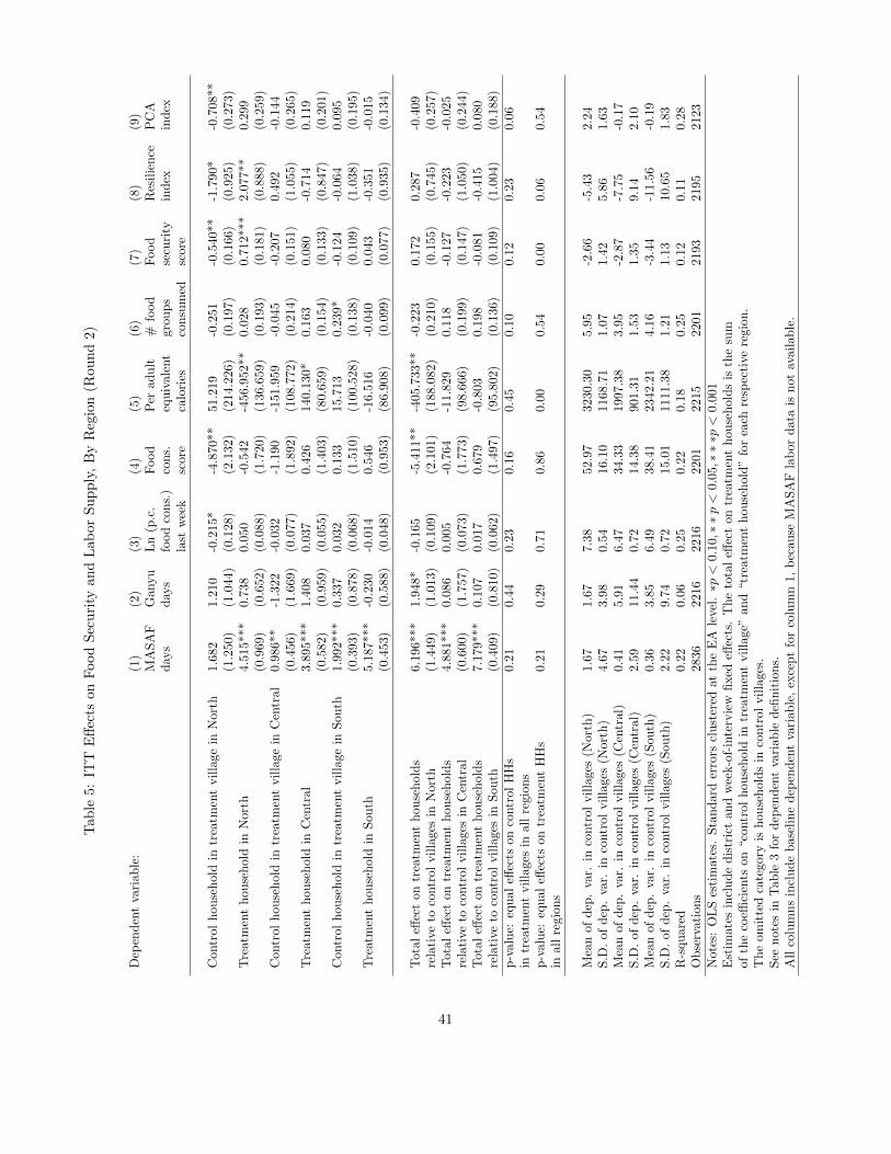
In Table 5, we report estimates of a fully interacted version of equation (1) in order

to understand whether the program was more effective in some regions than others, and to

consider whether regional variation provides any insight about the mechanisms for the effects

we find. The formatting of results is as follows: indirect and direct impacts (corresponding to

β1 and β2 in the pooled specification of equation 1) are reported separately for each region.

Then, we report the total effect on treated households separately for each region, followed by

p-values for tests that the indirect and direct effects are the same across the three regions.

The last panel of the table includes means and standard deviations of outcome variables

separately for each of the three regions.20

6.1 Lean season

Program participation among treated households is higher in the South (total treatment

effect of 7.1 days), followed by the North (6.4 days) and then the Central region (4.9 days),

though the differences across regions are not statistically significant (p=0.21, reported just

above dependent variable means). Treated households do not reduce their labor supply to

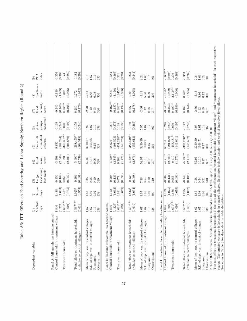
19Excluding the island district of Likoma20For specifications without the baseline value of the outcome variable, see Appendix Tables A6 – A8.

16

the private market in any of the regions; if anything, PWP crowds in employment in the

local casual labor market in the North, with households increasing the number of days of

ganyu.

The program has the most negative impact on food security in the North. Per capita

caloric intake falls by 406 calories per adult equivalent, a large and statistically significant

reduction that is statistically different from the direct effects on caloric intake in the other two

regions. The food consumption score falls by 5.4 points, representing a large and statistically

significant reduction (about 0.3 standard deviations relative to the control mean). However,

two other measures of food security improve for treated households relative to households

in control villages, albeit not significantly. The food security score improves by 0.172 points

(0.12 standard deviations) and households are slightly more resilient. Overall, the PCA index

falls by 0.41 points or 0.25 standard deviations relative to the control group and the food

consumption score falls by 5.4, though given the small sample size in the sparsely-populated

North, the change is not significant at standard confidence levels.

The indirect effect of the program in the North is quite pronounced. Untreated households

in PWP villages have worse food security than households in control villages for five of six

measures; reductions the food consumption score and food security are significant at the 95

percent confidence level, and reductions in per capita food consumption and resilience are

significant at the 90 percent level. The PCA index falls by 0.71 points or 0.43 standard

deviations relative to households in control villages in the region. That decline is significant

at the 95 percent level.

In the Central and Southern regions, the effects of the PWP are much smaller. For treated

households, there are no significant changes in any outcomes. The magnitude of the total

effect on the PCA index is close to zero in both the Central (-0.025) and Southern (0.080)

regions. Indirect effects are negative but not statistically significant for five of six outcomes

and the PCA index in the Central region. In the South, point estimates of the indirect effects

are close to zero for all outcomes except the number of food groups consumed, which records

a marginally significant increase. The small indirect effects in the Central and Southern

regions are a contrast to the substantial negative spillovers in the North. The p-value for

equal indirect effects on the PCA index is 0.06.21

The absence of household crowding out of employment in the local labor market across

regions and across different times of the agricultural season in Malawi stands in contrast

with the traditional public works literature where households are assumed to have to pay an

opportunity cost of participation (due to the foregone income) in public works programs. A

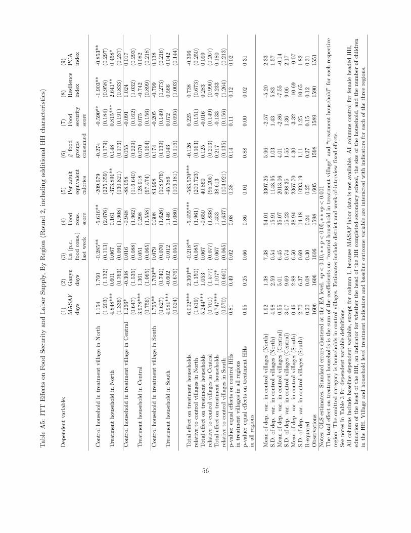
21Differences in the direct and indirect effects of PWP persist after controlling for observable baselinecharacteristics of households that may differ across regions. See Appendix Table A5 for estimates fromspecifications including the household characteristics reported in Table 2.

17

detailed analysis of the LSMS-ISA surveys in Tanzaia, Malawi, Ethiopia and Uganda testing

for the completeness in labor markets (Dillon, Brummund & Mwabu 2015) finds evidence of

a significant labor surplus in Malawi, in contrast with tighter labor markets like in Ethiopia.

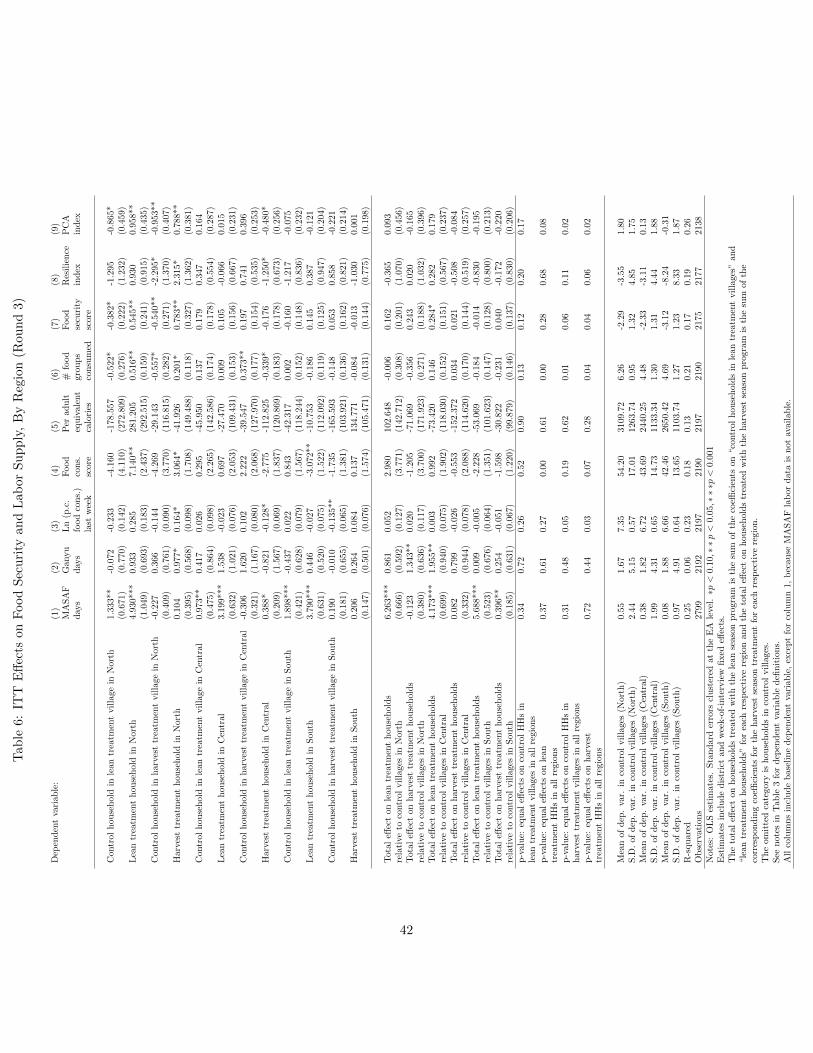
6.2 Pre-harvest period

As with the effects on lean season food security, estimating equation (2) on the full sample

obscures important regional heterogeneity. We report heterogeneous effects by region in Table

6. Participation in the lean season is high, with assignment to the lean season treatment

causing 6.3, 4.2, and 5.7 days of MASAF work in the Northern, Central, and Southern

regions respectively. While households treated with the lean season program work fewer

days in the Central region than in other parts of the country – mirroring the results for

planting season participation – the differences across region are not statistically significant

(p=0.37). By design, households treated with the harvest season program report almost no

work for MASAF in survey round 3. There is no evidence of crowding out of employment in

private labor markets. If anything, there are signs of crowding-in, with households increasing

their supply of ganyu labor. This happens in the North for treated households that were not

offered the program during the pre-harvest season, and for lean season treatment households

in the Central region.

In the North, the direct effect of the lean season program is small, with point estimates

that are positive for four of six outcomes and the PCA index. However, the program appears

to generate negative spillovers in this region. There are reductions in all six measures of food

security, with reductions in the number of food groups consumed and food security that are

significant at the 90 percent confidence level. The PCA index falls by 0.49 SD relative to

households in the control group, also marginally significant.

For those households in Northern villages who are yet to get the second cycle of 24 days

of PWP, outcomes are worse. The direct effect is negative or close to zero for most outcomes

and for the PCA index. The indirect effect that was estimated during the lean season persists

during the pre-harvest season: the estimated effect is negative for all outcomes, including

marginally significant reductions in dietary diversity and increases in both measures of food

insecurity. The negative effect on the PCA index is equivalent to 0.54 SDs of the control

group, and is statistically significant at the 95 percent confidence level. The negative spillovers

to untreated households that plagued the North in round 2 thus persist and deepen in round

3, and occur for both program variants.

In the Central region, the lean season program improves food security for both treated and

untreated households in PWP villages. The direct effect is positive for five of six outcomes

and the PCA index, which increases by 0.10 SDs though none of the differences relative

18

to households in the control villages are statistically significant at conventional levels. The

pattern and magnitude of indirect effects are similar: food security improves for five measures,

including an imprecisely estimated 0.09 SDs of the PCA index.

The impacts for households in the region that have yet to get the second 24-day cycle

(harvest season villages) are puzzling. The direct effects are, if anything, negative. Food

security falls along four of six measures, though none significantly. The magnitude of the

effect on the PCA index is negative but close to zero. The indirect effects, however, are

positive. Food security improves for five of six outcomes. The PCA index is 0.21 SD higher

for untreated households in villages with PWP than for households in control villages, though

the difference is not statistically significant. Since even the treated households did not work in

the period leading up to survey round 3 (but had 24 days of work opportunities in November-

January and will receive another 24 days beginning in May), it is conceivable that the indirect

effects are due to anticipatory behavior by untreated households who are not on the cusp of

another 24 day work cycle, relative to treated households whose next work opportunity is

pending.

Finally, the lack of effects of PWP in the South that we observed in survey round 2

continues in survey round 3. For the lean season program, the pattern of direct effects is

not encouraging: food security fell for five of six outcomes; the PCA index declined by 0.195

points or 0.10 SD, though the change is not statistically significant. The indirect effects are

even smaller in magnitude, with the point estimate of the indirect effect on the PCA index

close to zero. The harvest season program (villages awaiting their next 24-day work cycle)

has negative direct effects on food security on five of six outcomes and reduces the PCA

index by 0.12 SDs; none of the changes are significant. The indirect effects are negative but

not significant for four of six outcomes. The decline in the PCA index is -0.12 SDs.

For each of the three regions, we test that the direct effect of the lean season program

(where treated households were offered 48 days of work as of survey round 3) equals the direct

effect of the harvest season program (which offered 24 days of work before survey round 3),

and that the corresponding indirect effects are equal. We fail to reject the equality of the two

program variants for most outcomes, but the overall pattern of results for food security in

all three regions is more favorable – or at least less damaging – for the lean season program

(which offered 48 days of PWP) than the harvest season program (as yet offered 24 days of

PWP). We do find statistical evidence of differences across the three region, rejecting equal

direct effects on the PCA index of either the lean or harvest season treatments, respectively,

in all three regions (p=0.08 for the lean season treatment and 0.02 for the harvest treatment)

or equal spillovers due to the harvest treatment (p=0.02).

19

6.3 Interpreting regional differences

The overall pattern of results in Table 5 suggests that the PWP was less effective – or

potentially even slightly harmful – during the lean season in the North than in the other

regions of the country. The direct effect of participation in the program was negative and

significant for two of the seven food security outcomes in the North. Yet, we cannot reject

the null hypothesis of equal effects on the PCA index for treated households during the lean

season in all three regions (p=0.54, Table 5).

However, for five of the seven food security measures, control households in treatment

villages in the North were significantly worse off after the program. And we can reject the null

hypothesis of such equal indirect effects on the PCA index (p=0.06, Table 5). Unfortunately,

as we discuss in Section 8, it is challenging to identify a mechanism for these negative indirect

effects, or why the indirect effects would be different across regions. This result is not due to

differences in the distribution of baseline characteristics across the three regions; the regional

differences persist, though remain imprecisely estimated for many outcomes, in specifications

that interact treatment indicators with baseline characteristics.22 We have no reason to

believe that the program was implemented differently in the North than in other regions;

and, if anything, it was better-targeted in the North. With only three regions, we cannot

formally test whether differences in aggregate conditions in the regions explain the differences

in indirect effects.

Further complicating the interpretation of regional differences, the direct effects of the

PWP in the pre-harvest period, as reported in Table 6, are not worse in the North than in the

other regions. However, the indirect effects of both the lean and harvest treatment programs

are large, negative, and statistically significant in the North, and as reported in the previous

section, we reject the null that the indirect effects of the harvest treatment are equal in all

three regions.

With a larger sample size that allowed us to exploit aggregate variation at a sub-region

(Traditional Authority) level, we might be able to formally test whether regional differences

in accessibility, population density or features of local labor, agriculture and goods markets,

drive some of these findings. Given the sample for this study, however, we are limited

to simply observing that there is no region in which PWP has clear positive effects, and

particular caution should be exercised when implementing it in the North.

22Results available upon request

20

7 Use of fertilizer

Complementarities with the fertilizer subsidy scheme drive the design of the program, and

increased fertilizer use is a major stated goal of the PWP. In Malawi, fertilizer is applied

twice to both maize (the staple crop) and tobacco (the main cash crop). Since survey round

2 captures fertilizer applied during planting season, we estimate equation (1) to investigate

the effect of the program on the use of fertilizer. We examine the probability that a household

uses any chemical fertilizer during the 2012/13 season; the log of expenditure on fertilizer

for the first and second applications; and the log of the quantity of fertilizer used in the

first and second applications. For the expenditure and quantity variables, we use the inverse

hyperbolic sine transformation to be able to take logs of variables where some observations

are zeros. These results are reported in the first five columns of Table 7. The national point

estimates of both the direct and indirect effects on any of these outcomes are close to zero,

and none of the coefficients are statistically significant.

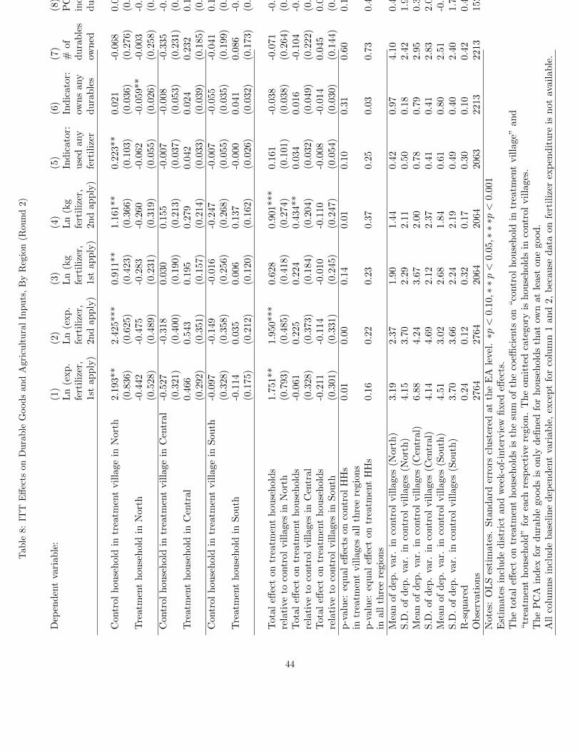
However, the results reported in Table 8 indicate important heterogeneity by region:

while fertilizer use is generally unchanged in the Central and Southern regions, it increases

for both treated and untreated households in PWP villages compared to non-PWP villages

in the North. In fact, control households in PWP villages use more fertilizer than their

directly-treated counterparts, though the difference between the two groups is not statisti-

cally significant. They are significantly more likely to use fertilizer (22.3 percentage points,

column 5), use significantly larger quantities, and spend significantly more on fertilizer than

households in control villages. For the treated households, the quantity of fertilizer used in

both applications and expenditures for the second application increase significantly relative

to households in control villages. Increased use of fertilizer cannot affect food security during

the lean season, but might translate into higher yields several months later.

8 Mechanisms

Malawi’s PWP increases potential household income by providing paid work, if not offset by

reductions in other labor supply. Despite this, households offered PWP do not have better

food security or use more agricultural inputs as a result of the program, and food security

either does not improve or worsens among untreated households in PWP villages. We discuss

and, when possible, test potential mechanisms for the lack of positive direct effects, and for

the negative spillovers in the Northern and Central regions.

21

8.1 Study design

8.1.1 Low power

Lack of statistical power is one possible explanation for a null main effect. It would be a

more plausible explanation had we found positive but imprecisely estimated point estimates,

however. Instead, we find predominantly negative effects that are not statistically different

from zero. This is true not only at the national level, but also within each region.

We consider the confidence interval for the effect on treated households in order to assess

the magnitude of impacts, focusing on the lean season. We can rule out meaningful positive

effects of the program: nationally, the upper bound (at the 95 percent confidence level) of

the improvement in food security for five of the six individual indicators is less than 0.2

standard deviations of the outcome in the control group; for the sixth, the number of food

groups consumed, the upper bound of the confidence interval is 0.22 standard deviations. The

standard deviation of the PCA index for food security is 2.08, and the confidence interval for

the effect of the PWP on treated households is [-0.29, 0.24].

By region, the upper bound of the 95 percent confidence interval for any individual

outcome is 0.34 SDs in the North, 0.33 SDs in the Center, and 0.38 SDs in the South. For

the PCA index, the upper bound of the effect is 0.06 SDs in the North, 0.22 SDs in the Center,

and 0.24 SDs in the South. Thus, even moderate direct effects are outside the confidence

intervals in each region. It does not appear that lack of statistical power explains the lack of

positive effects of the program.

8.1.2 Low take-up

The second possibility is that the household-level intervention, which chose households for

inclusion in PWP at random, resulted in low take-up and therefore small ITT estimates. The

ITT estimates are not biased, but they are – by construction – smaller in absolute value than

the TOT effects. Since assignment to the treatment group increases PWP participation, the

TOT and ITT effects have the same sign. Therefore, discussion of the TOT does not offer

an explanation for coefficients with unanticipated direction of impact.

As designed and implemented by the government, the program is targeted at vulnera-

ble households, which might participate at higher rates than randomly selected households.

Across the full study, 57 percent of treated (that is, randomly-selected) households in our

study participated in PWP.23 Since there are considerable within-village spillovers, using

household treatment status as an instrument violates the stable unit treatment value as-

sumption (SUTVA) and is not a valid specification. Instead, we can instrument for PWP

23See Table A9 for participation rates by round.

22

participation using village randomization, where the first stage equation is

Any PWP participationiv = δ0 + δ1PWPv + Γd + Θt + νiv (3)

In this specification, the treatment effect incorporates direct and within-village spillover

effects; the assumption is that there are no across-village spillovers within our sample, and

this is justified by the distance between study villages. Participation is less than 100 % by

design: δ1 = 0.34, and the first stage F-statistic is 186.07. The national TOT parameters

reported in Table A10 are larger in magnitude than the weighted average of the direct and

indirect effects reported in Table 4, but imprecisely estimated and always in the direction of

reducing food security.

Participation varies somewhat by region at 58 percent of treated households in the North,

43 percent in the Center, and 65 percent in the South (see Table A9). Regional TOT estimates

are reported in Appendix Table ?? and indicate worse food security for PWP participants

in all regions. Low take-up does not explain the lack of impact of PWP on food security.

8.2 Design of PWP

8.2.1 Value of transfer

A key design feature that may contribute to the lack of a direct effect is the low total value

of PWP income. The wage rate for the program was set by the government at MK 300

($0.92) per day, with total possible earnings of MK 14,400 ($44.16). The wage rate is low

by international standards, but, in a country with gross national income per capita of $320

($730, adjusted for purchasing power parity), $44 is non-trivial. The payment for a 12-day

work period (the amount disbursed by the government in each pay parade) is equal to the

value of mean weekly food consumption at baseline (and more than 1.5 times weekly food

expenditure).

Local political constraints made it infeasible to vary the wage rate for this study; so,

our experimental design does not allow us to speak to the effect of PWP with higher wages.

Despite extensive consumption and expenditure data in our surveys, we are not able to

detect increases in any category: food, agricultural inputs or business investments, non-food

consumption, or durables. This limitation is shared with many studies on microfinance,

which similarly fail to detect the effect of increased cash on household consumption and

expenditures.

The lack of beneficial effects of the additional 24 days of work during the lean season also

undermines the idea that a more generous program would transform the effects. Treated

households in villages selected for the lean season treatment were eligible for 24 additional

23

days of work in March (for a total of 48 days from November to March). Yet, in surveys

conducted the following month, their food security is no better than either households in

control villages or treated households in the harvest season villages (offered 24 days from

November to January).

8.2.2 Timing

A second hypothesis related to the design of the PWP program concerns timing of the

program. First, the program covers periods where the opportunity cost of time is potentially

high. Perhaps work on PWP activities crowded out the labor supplied to the household

farms or to the wage labor market. We do not have data about hours of work in household

agriculture, but note that since survey round 2 is conducted before the harvest, any reduction

in food security due to reduced future harvests cannot explain the results and would instead

exacerbate the zero or negative effect on food security measured later in the year.

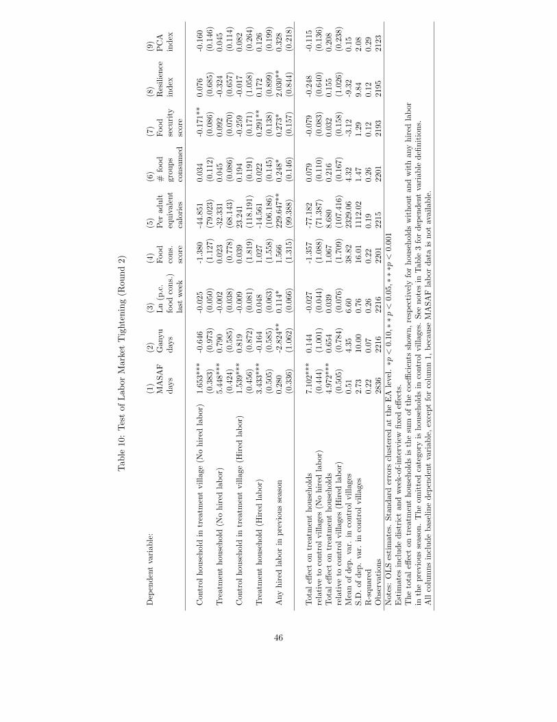
As discussed above, we report the effect of the PWP on labor supply in daily wage mar-

kets(ganyu) in Table 4 (columns 8 and 9). Both the direct and indirect effects of the program

are small and not statistically significant at the extensive margin of participation (not shown);

at the intensive margin, PWP, if anything, crowds in wage labor, though standard errors are

large. It appears that households have an excess supply of labor, a finding consistent with

Goldberg (2016).

It also seems unlikely that poor timing vis a vis other government programs explains the

results. PWP and the fertilizer subsidy are administered separately and are not perfectly

synchronized. The planting season begins earlier in the South than in the North, and the

government activated PWP activities earlier in the South. In three study districts, fertilizer

subsidy coupon distribution took place between the first and second 12-day waves of PWP

activities, and, in the remaining nine districts, fertilizer coupon distribution overlapped with

PWP work and payment. The three districts without overlap were Blantyre (South), Dowa

(Center), and Karonga (North). The North accounts for a smaller fraction of total population

and therefore of our sample; so, discordant timing in one study district represents a larger

share of beneficiaries in that region than in the Center or South.

8.2.3 Targeting

Regressive or ineffective targeting potentially explains both lack of direct effects and nega-

tive indirect effects. PWP is intended for the able-bodied poor and uses a combination of

community wealth ranking exercises and low wages to target the program. In practice, the

characteristics of participants may differ from the eligibility criteria because of differences in

how local officials select beneficiaries and in the opportunity cost of participation. There are

24

two types of targeting that may modulate impacts. The first is the selection of village-chosen

beneficiaries. As noted above, some untreated households in our study were village-chosen

beneficiaries. We examine the correlation between baseline per capita food consumption and

participation of these households as an indication of whether the village selection procedures

targeted poorer households. Our preferred measure of baseline food security comes from the

IHS3 because, unlike round 1 of the evaluation data, the IHS3 data were collected before the

intervention was announced. We cannot assess targeting on short-term food security because

survey round 1 data were collected after the program was announced and may be affected by

anticipated PWP earnings. However, if PWP is used locally in response to short-term shocks,

the lag between the IHS3 and program implementation may explain the lack of correlation

between time-varying characteristics such as food security and participation.

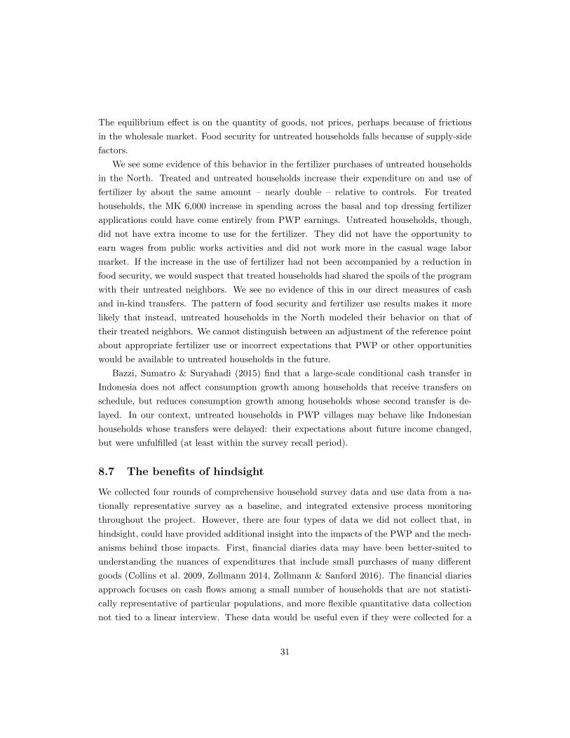
Nationally, Figure 3 illustrates that there is very correlation between food security in

2010/11 and participation through the village selection process. This may suggest that the

village selection process either responds to short-term food security or relies on criteria that

are orthogonal to long-term consumption.24

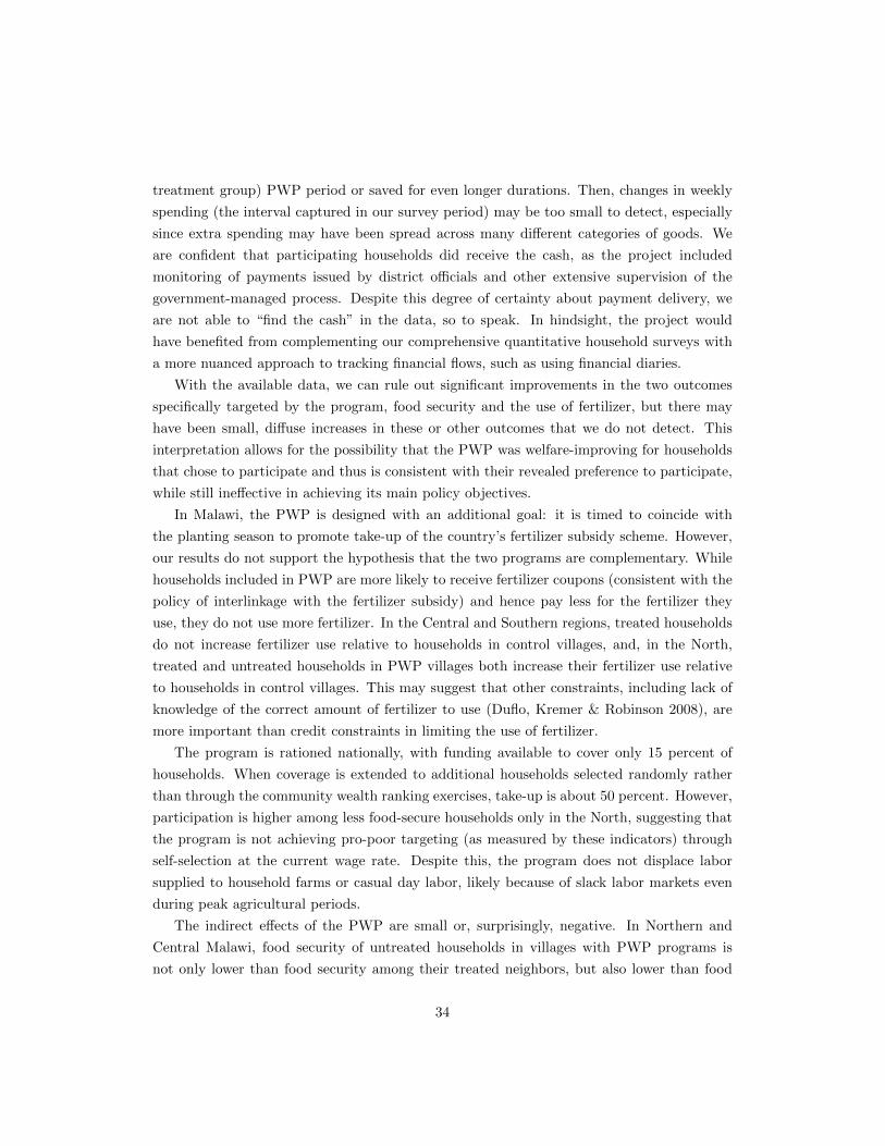
As shown in Figure 4, the relationship between food security and PWP participation

varies by region. In the North and Central regions, participation of untreated households

was uniform across the distribution of baseline food consumption.25 In the South, households

with lower baseline food consumption were, if anything, less likely to be chosen by GVH and

participate in PWP.

The second type of targeting is self-targeting, captured by participation by randomly

selected households from different points of the distribution of baseline food consumption.

This mimics an unrationed PWP such as NREGA. Among treated households, the correlation

between accepting PWP work and IHS3 food consumption is negative in the North (indicating

pro-poor targeting and self-selection of the poorest households), but not in the Central or

Southern regions. Though self-targeting seems more prevalent in the North, there is no

evidence of displacement of casual wage labor (ganyu) in any region.

Overall, Malawi’s PWP is rationed and not very well targeted toward the food insecure.

Mistargeting could explain the lack of improvement in food security if the program employed

people who had lower marginal propensity to consume food, but the geographic heterogeneity

in targeting does not seem to explain the regional heterogeneity in results. PWP was, if

anything, slightly better targeted in the region where it led to the most pronounced negative

spillovers.

24The autocorrelation between log per capita food consumption in the IHS3 and survey round 1 in controlvillages is 0.30. Over shorter horizons, between any two adjacent survey rounds, the autocorrelation in controlvillages is close to 0.5.

25Food consumption data from the IHS3, accounting for seasonality by detrending by week-of-interview.

25

8.2.4 Project type

PWP activities included road building and tree-planting, which conceptually could have

required different effort levels or induced differential selection by participants. While project

type is unlikely to explain the lack of direct effect, different project types across the three

regions could lead to heterogeneous effects. In fact, the mix of projects was similar across the

three regions. We have limited anecdotal information about the day-to-day work activities

of beneficiaries, with no evidence of systematic differences by region. As discussed above,

PWP activities do not displace wage work in any region. We conclude that any differences

in work activities are unlikely to explain regional differences in program impacts.

8.3 Equilibrium effects

8.3.1 Prices

Spillovers could operate through goods markets. If increased demand by treated households

drove up the price of food or other goods, the program may have reduced the purchasing

power of both treated households and their untreated neighbors. A change in price level has

the potential to explain both the lack of positive effects for treated households and negative

effects on their untreated neighbors, though differences in market conditions across the three

regions would be necessary to explain why the negative spillovers were observed in the North

and Central regions, but not the South.

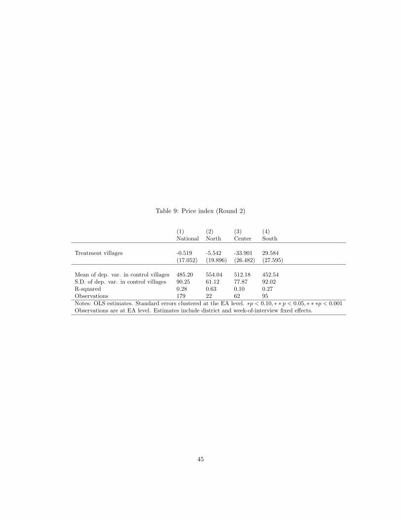
We test whether village-level prices were different in treatment and control villages us-

ing a price index constructed from households’ reported prices for the five most commonly

purchased goods. The specification for village-level differences is

yv = α+ βPWPv + Γd + Θt + εv (4)

Note that this specification estimates the effect of PWP on prices at the coverage rate in

the experiment. As reported in Table 9, the difference in the price index between treatment

and control villages is neither economically nor statistically significant. Nationally, prices

in treatment villages are nearly identical – within one percent – to those in control villages.

Neither is there any evidence of price effects at the regional level. In the North, the magnitude

of the coefficient on the PWP indicator is near zero; prices are about seven percent lower

for treatment villages than controls in the Center and seven percent higher in the South.

None of the differences are statistically significant. This likely reflects the low coverage rate

of PWP.

26

8.3.2 Labor markets

Imbert & Papp (2015) find that the large Indian PWP increases wages in the low-skill market.

A similar effect on equilibrium wages in Malawi could explain negative externalities by driving

up labor costs for untreated households that hire workers, especially since planting season

PWP activities coincide with peak labor demand. There was not substitution away from

work in the private wage market in Malawi, but the PWP program could have driven up

reservation wages.

We did not collect data about wages paid for hired labor. To test the labor market

tightening hypothesis indirectly, we interact the PWP treatment variables with an indicator

for whether the household reported hiring any agricultural labor in the IHS3; about 20

percent of households had previously hired labor.

We estimate

yiv =α+ ψ1PWP, no hired laboriv + ψ2PWP, hired laboriv

+ ψ3PWP, no hired laboriv ∗ Topupi + ψ4PWP, hired laboriv ∗ Topupi

+ ψ5Any previous hired labori + Γd + Θt + εiv

(5)

ψ1 is the indirect effect of PWP on households that did not hire any labor during the 2010/11

growing season, and ψ2 is the indirect effect on households that did. If labor market tightening

were responsible for negative spillover effects, we would expect ψ2 to be negative (and more

negative than ψ1).

Instead, as reported in Table 10, the indirect effect of PWP is negative for households that

do not hire, a group that might benefit from, and should not be harmed by, higher equilibrium

wages. For the PCA index (column 9), the point estimate of ψ1 is -0.16, not statistically

different from zero at conventional levels but substantial relative to the mean in the control

group (0.15). The indirect effect on households that previously hired labor and would face

higher costs due to an increase in wages is positive though smaller in magnitude: ψ̂2 = 0.08.

This test does not support the labor market tightening channel (via wage increases) for the

negative spillovers.

8.4 Changes in transfers from institutions or individuals

Other institutions – governmental or nongovernmental programs – or individuals could have

changed their behavior towards untreated households or otherwise compensated control vil-

lages with other programs. In this case, the untreated households in PWP villages, which

benefited from neither PWP nor these alternative programs, may be worse in comparison.

We have data about the receipt of five types of benefits: food assistance or maize distribution,

27

school-based nutrition programs, scholarships or other help with school fees, cash transfers,

and fertilizer coupons. As shown in Table 11, there is no evidence that untreated households

differ in their receipt of these benefits from either treated households or households in control

villages. (Indeed, the only economically or statistically meaningful difference is in fertilizer

coupons, which are more likely to be available to treated households in accordance with the

designed linkage between PWP and the national fertilizer subsidy scheme.)

A related hypothesis is that treated households were not the final beneficiaries of the pro-

gram, but instead shared their income with other households or used it to replace or repay

loans. We examine four outcomes in the right hand side of Table 11: whether the household

received any transfers, whether it made any transfers to others, whether it received any new

loans, and whether it made any loan payments in the previous month. Both treated house-

holds and untreated households in PWP villages give fewer transfers than their counterparts

in control villages, which works against explaining the main findings. PWP does not have a

significant direct effect on other transfer outcomes, and the magnitudes of the direct effects

are small as well as imprecisely estimated.

It is also possible that contacts reduced transfers to or increased demands for transfers

from households in villages with PWP. Even untreated households in PWP villages could be

affected through this channel. For example, family members living in other locations may

know that PWP was active in a village, but have inaccurate information about who actually

benefited from the program. They may falsely believe that untreated households received

income from PWP and therefore do not need support through social networks or may even

have funds they could share with others. The results reported in columns (6) through (9) of

Table 11 indicate that untreated households are significantly less likely than households in

control villages to make transfers to others, ruling out the possibility of misguided pressure

to share income. Untreated households do not significantly differ from controls (or treated

households) in their probabilities of receiving transfers or accessing loans, and the effects are

not different across the three regions.

8.5 Behavioral responses by treated and untreated households

Finally, households offered PWP may make choices that offset or limit the effect on food se-

curity. If households behave according to the predictions of the permanent income hypothesis

(PIH), then the temporary increase in income will be allocated to consumption in all future

periods, and the change in consumption in any one period would be diminishingly small,

as in Chen, Mu & Ravallion (2009). This could account for the lack of positive effects on

the food security of treated households, but cannot explain negative spillovers to untreated

households. Perhaps more importantly, the myriad credit market imperfections in Malawi

28

that lead to well-documented seasonal variation in consumption make it unlikely that the

PIH holds in this context.

Another possibility is that treated households responded to the program by voluntarily

reducing their food consumption to pool existing resources and wages from the program and

make indivisible purchases of durables. We test this hypothesis by estimating the effect of

PWP on durable ownership (Table 7, columns 6-8). We consider three measures of durable

ownership: the probability of owning at least one of 32 goods covered in the survey, the total

number of durable goods owned, and a PCA index of durable ownership. The total effect

of PWP on treated households is not significantly different from zero for any of the three

outcomes, and the imprecise estimates for the number of goods and PCA index are negative.

There is no evidence that households offered PWP use program earnings or other resources

to purchase durable goods, and these effects do not differ by region (Table 8).

Recall both treated and spillover control households in the North do increase their use of

fertilizer. The negative direct and indirect effects on food security are also most pronounced

in the North. Households in that region may have devoted PWP income and other resources

to the purchase of fertilizer rather than the purchase of food. We highlight this result because

it is the only evidence we have of behavior that is consistent with the unexpected negative

spillovers on food security and matches the geographic pattern of direct and indirect results.

8.6 Remaining possibilities

While the PWP increased income for treated households, it may simply have been too small or

too poorly timed to measurably improve their food security or to increase their use of fertilizer.

An explanation for the secondary finding of negative spillovers to untreated households is

more elusive. Here, we discuss the remaining possibilities to complete our consideration of

our findings.

One possible explanation for negative spillover effects is strategic self-reporting by un-

treated households that do not experience real reductions in food security, but choose to

underreport consumption to signal their potential eligibility and increase their chances of

being offered PWP or other benefits in the future. If strategic misreporting were responsible

for finding negative spillovers, then perhaps it also biased the estimate of the main effect.

We argue that two features of our research design make it unlikely. First, data collection and

program implementation were conducted by different institutions. The NSO was responsi-

ble for survey work, and the Local Development Fund, with assistance from Innovations for

Poverty Action, managed PWP activities and payments. Respondents did not report their

food consumption or other outcomes to people who were employed by or connected to the

administration of the PWP. Second, the IHS3 households in our study were part of a na-

29

tionally representative survey that is not connected to the provision of any public or private

benefits. These households had been administered the same survey instrument by the same

institution (NSO) before the study began and had not received any benefits that depended

on their answers. These features distinguish our evaluation from randomized controlled tri-

als that rely on data collected by employees of the same organization that administers the

intervention, and from evaluations of subjects who may infer that surveys are collected for

the purpose of allocating benefits.

We are not able to assess the reliability of our outcome measures to determine whether

perceived or self-reported food security may have fallen, absent a change in objective con-

sumption. While the eight different measures of nutrition we examine are all related to

food security, they measure different aspects of the concept. Therefore, we cannot use the

correlations between items in the IHS3 and subsequent survey rounds as an indication of

item reliability, because the program itself may have affected some measures of food security

differently than others.

We cannot rule out that PWP changed the behavior of untreated households in some

way that worsened food security. Such a mechanism would have to take a specific form to

explain both the main effect and the indirect effects, and be consistent with other behaviors

we observe. One possibility is as follows: PWP eligibility causes a change in the behavior of

treated households that is not captured by our survey (either because it falls outside the recall

period, or because it is too small to be measured precisely). Untreated households respond to

the behavior or consequences of the behavior by the treated households. For example, treated

households might spend their earnings by increasing consumption immediately after payment,

which would not be captured by a the seven-day recall period of the survey that takes place a

few weeks after the payment. Untreated households respond by similarly increasing short-run

consumption to keep up with their neighbors or because their reference point was affected, but

then have to reduce consumption in subsequent periods because their short-term splurge was

not financed by PWP earnings. This explanation requires peculiar behavior by the untreated

households, however: their marginal utility of keeping up with their neighbors is high enough

to offset reduced consumption later on, or their preferences are time inconsistent, or they

have erroneous expectations about future income. This sort of conspicuous consumption with

negative welfare consequences has been documented among neighbors of Canadian lottery

winners (Agarwal, Mikhed & Scholnick 2016).

An alternative explanation requiring less complicated behavior by the untreated house-

holds is that, immediately after they are paid, treated households purchase food in bulk

quantities for storage and later consumption. These purchases are not captured in the sur-

vey recall period and therefore do not translate into increased food security from the program,

but they do reduce the availability of commodities at local markets for untreated households.

30

The equilibrium effect is on the quantity of goods, not prices, perhaps because of frictions

in the wholesale market. Food security for untreated households falls because of supply-side

factors.

We see some evidence of this behavior in the fertilizer purchases of untreated households

in the North. Treated and untreated households increase their expenditure on and use of

fertilizer by about the same amount – nearly double – relative to controls. For treated

households, the MK 6,000 increase in spending across the basal and top dressing fertilizer

applications could have come entirely from PWP earnings. Untreated households, though,

did not have extra income to use for the fertilizer. They did not have the opportunity to

earn wages from public works activities and did not work more in the casual wage labor

market. If the increase in the use of fertilizer had not been accompanied by a reduction in

food security, we would suspect that treated households had shared the spoils of the program

with their untreated neighbors. We see no evidence of this in our direct measures of cash

and in-kind transfers. The pattern of food security and fertilizer use results makes it more

likely that instead, untreated households in the North modeled their behavior on that of

their treated neighbors. We cannot distinguish between an adjustment of the reference point

about appropriate fertilizer use or incorrect expectations that PWP or other opportunities

would be available to untreated households in the future.

Bazzi, Sumatro & Suryahadi (2015) find that a large-scale conditional cash transfer in

Indonesia does not affect consumption growth among households that receive transfers on

schedule, but reduces consumption growth among households whose second transfer is de-

layed. In our context, untreated households in PWP villages may behave like Indonesian

households whose transfers were delayed: their expectations about future income changed,

but were unfulfilled (at least within the survey recall period).

8.7 The benefits of hindsight

We collected four rounds of comprehensive household survey data and use data from a na-

tionally representative survey as a baseline, and integrated extensive process monitoring

throughout the project. However, there are four types of data we did not collect that, in

hindsight, could have provided additional insight into the impacts of the PWP and the mech-

anisms behind those impacts. First, financial diaries data may have been better-suited to

understanding the nuances of expenditures that include small purchases of many different

goods (Collins et al. 2009, Zollmann 2014, Zollmann & Sanford 2016). The financial diaries

approach focuses on cash flows among a small number of households that are not statisti-

cally representative of particular populations, and more flexible quantitative data collection

not tied to a linear interview. These data would be useful even if they were collected for a

31

stratified subsample of the population, and in a multi-round project like this, results from

financial diaries collected early in the project could have been used to adjust the question-

naires used in subsequent survey rounds. Because our process monitoring leaves us confident

that respondents received cash, data that would help us understand where it went are the

top priority.

We think concerns about strategic misreporting are unlikely to explain our findings be-

cause of the separation between data collection and program implementation and because

it is commonly known in Malawi that villages do not participate in the PWP in successive

years. That said, the second type of data that could help alleviate remaining concerns include

objective measures of physical wellbeing or other outcomes.

For example, data about soil nitrogen levels could be used as a proxy for fertilizer ap-

plication. Anthropometric data (weight, mid upper-arm circumference, or even biomarkers

such as hemoglobin levels) could have provided a direct test of the effect of the program

on physical wellbeing (Frankenberg, Ho & Thomas 2016). These data are not subject to

concerns about recall or reporting error, and can capture outcomes that are hard to observe

from household survey data when resources are not divided equally or predictably among

household members. Anthropometric data can be measured quickly and accurately with

proper training, but they are also notoriously slow to change. In assessing the benefits of

large scale programs like PWPs, a reasonable strategy to contain costs and maximize power

might involve collecting outcomes for individuals who are expected to be most sensitive to

short-term changes in food availability, such as acute malnutrition in young children.

Haushofer & Shapiro (2016) complement self-reported wellbeing by measuring the stress

hormone cortisol. This could offset concerns about strategic misreporting of wellbeing,

though stress is only one mechanism through which PWPs could affect happiness.

Third, measures of subjective wellbeing would have been helpful in interpreting the re-

sults. Questions on mental health and psychological distress as well as expectation about

the future could help to determine whether benefits accrued through a different channel than

consumption. A decrease in subjective wellbeing would, of course, support the conclusion

that the program does not make participants better off.

Fourth, conducting the household surveys closer to the payment day, such that the sur-

vey recall period included the day of the payment, would detect very short-run changes in

expenditures and consumption and rule out the “keeping up with the Joneses” hypothesis

discussed in the previous section. While this would rule out one possible explanation for the

results we obtain, it is not clear that outcomes only at the moment of payment are of interest

when evaluating a program with infrequent payments that is nonetheless designed to smooth

consumption. A comprehensive data collection strategy might include weekly consumption

and time-use surveys, in order to measure contemporaneous and post-program effects, and

32

to improve statistical power with highly correlated outcomes (McKenzie 2012).

Finally, leveraging nationally representative survey data increased the statistical power

for this project and provides a public good: panel data that we expect to be of use to other

researchers. Such a strategy is logistically demanding and required that we cede control

of some of the day-to-day aspects of data collection to the National Statistics Office. In

our case, this led to delays and missing baseline data for some villages. We consider the

tradeoff worthwhile, both because of the rich data available to this and other projects, and

because of the separation between the implementation and data collection associated with

this evaluation.

9 Conclusion

PWPs can stabilize the income and improve the food security of beneficiaries by providing

earnings opportunities, and can achieve targeting through low wages and work requirements

that promote self-selection. While Malawi’s PWP offers households the opportunity to earn

approximately $22 at planting season and an additional $22 later in the year, it does not have

a measurable short-term effect on lean season food security. Even improving the structure

of the program by rescheduling the second work cycle from the harvest season to the lean

season does not generate measurable improvements in the food security of treated households.

These findings stand in contrast to those from large PWPs in India and Ethiopia, and serves

as a reminder that PWPs will not always have significant and measurable welfare effects.

While the maximum possible income from PWP is substantial in light of the country’s

per capita gross national income of $320, the magnitude of the transfer is low compared

with other social protection tools such, as cash transfers being studied in Malawi,26 or other

PWP programs in Sub-Saharan Africa.27 Our results do not speak directly to the effect

of a more generous program, though comparison with results in other countries suggests

potential earnings as a margin for increasing the impact of the program. Perhaps because

of the low daily wage in MASAF’s PWP, 24 extra days of work during the lean season does

not significantly improve food security, but longer duration and more flexible schedules are

avenues for future investigation.

Households may have spread consumption across the four- to eight-month (depending on

26In their study of the cash transfer project in one district of Malawi in 2007, Miller, Tsoka & Reichert(2011) find large, positive effects on beneficiary households in program villages compared with householdsin control villages screened as eligible but not given the program. In this program, the size of the benefit issignificantly larger, with transfers totaling $168 per household over the course of a year (equivalent to about$250 in 2012 price levels), an amount more than five times what households received from PWP in 2012/13.

27Comparable PWP programs in the region, such as the ones in Ethiopia, Sierra Leone, and Ghana, havemaximum earnings of between $60 and $190.

33

treatment group) PWP period or saved for even longer durations. Then, changes in weekly

spending (the interval captured in our survey period) may be too small to detect, especially

since extra spending may have been spread across many different categories of goods. We

are confident that participating households did receive the cash, as the project included

monitoring of payments issued by district officials and other extensive supervision of the

government-managed process. Despite this degree of certainty about payment delivery, we

are not able to “find the cash” in the data, so to speak. In hindsight, the project would

have benefited from complementing our comprehensive quantitative household surveys with

a more nuanced approach to tracking financial flows, such as using financial diaries.

With the available data, we can rule out significant improvements in the two outcomes

specifically targeted by the program, food security and the use of fertilizer, but there may

have been small, diffuse increases in these or other outcomes that we do not detect. This

interpretation allows for the possibility that the PWP was welfare-improving for households

that chose to participate and thus is consistent with their revealed preference to participate,

while still ineffective in achieving its main policy objectives.

In Malawi, the PWP is designed with an additional goal: it is timed to coincide with

the planting season to promote take-up of the country’s fertilizer subsidy scheme. However,

our results do not support the hypothesis that the two programs are complementary. While

households included in PWP are more likely to receive fertilizer coupons (consistent with the

policy of interlinkage with the fertilizer subsidy) and hence pay less for the fertilizer they

use, they do not use more fertilizer. In the Central and Southern regions, treated households

do not increase fertilizer use relative to households in control villages, and, in the North,

treated and untreated households in PWP villages both increase their fertilizer use relative

to households in control villages. This may suggest that other constraints, including lack of

knowledge of the correct amount of fertilizer to use (Duflo, Kremer & Robinson 2008), are

more important than credit constraints in limiting the use of fertilizer.

The program is rationed nationally, with funding available to cover only 15 percent of

households. When coverage is extended to additional households selected randomly rather

than through the community wealth ranking exercises, take-up is about 50 percent. However,

participation is higher among less food-secure households only in the North, suggesting that

the program is not achieving pro-poor targeting (as measured by these indicators) through

self-selection at the current wage rate. Despite this, the program does not displace labor

supplied to household farms or casual day labor, likely because of slack labor markets even

during peak agricultural periods.

The indirect effects of the PWP are small or, surprisingly, negative. In Northern and

Central Malawi, food security of untreated households in villages with PWP programs is

not only lower than food security among their treated neighbors, but also lower than food

34

security in control villages without PWP activities. This is in contrast to expectations

and to the effects of other large-scale transfer programs. For example, Oportunidades, the

conditional cash transfer program in Mexico, generated positive effects on the consumption

of treated households and positive externalities to non-beneficiary households (Angelucci &

DeGiorgi 2009).

An explanation for this unexpected finding has proven elusive. Cash transfers in Mexico

generated equilibrium effects on commodity prices (Cunha, DeGiorgi & Jayachandran 2014),

but we find no evidence of price increases in Malawian villages with PWP. The large PWP

in India raised equilibrium wages, but we reject the labor market tightening explanation for

negative spillovers in Malawi. Pressure to share money could have explained the negative

effect on untreated households if relatives mistakenly believed that, because PWP was present

in the village, even the untreated households had benefited and could contribute to the social

network. However, there is no evidence of increased income sharing from PWP villages, and,

if anything, untreated households made fewer contributions to their networks than households

in control villages.

A possibility we cannot exclude is that untreated households reduce food consumption in

reaction to an unobserved change in the behavior of treated households or to erroneous expec-

tations of their own future income. We discuss two examples of this: untreated households

overspend to match a short-term and thus, unobserved (by the econometrician) increase in

consumption by their treated neighbors, and compensate by reducing consumption during

the period we do observe, or a combination of stock-outs and sticky prices reduces food

availability. The matching and substantial increases in fertilizer use by both treated and

untreated households in the North, the region with the strongest negative spillovers, are con-

sistent with this hypothesis. We lack direct evidence to test related behaviors, but present

them as examples of the types of mechanisms that could explain the unexpected finding

that Malawi’s PWP reduces the food security of untreated households in villages with PWP

activities. Identifying the mechanism remains a priority for both understanding household

spending patterns and informing policy.

35

Figures

Figure 1: Experimental design

Treatment at the community levelCycle 1: Planting season PWP Cycle 1: Planting season PWPCycle 2: Harvest season PWP Cycle 2: Lean season PWP

No PWP Group 0[38 communities]

PWP with lump sum payment Group 1 (status quo) Group 3[40 communities] [35 communities]

PWP with split payment Group 2 Group 4[34 communities] [35 communities]

Figure 2: Timeline

Year-round Pre-planting Planting Lean Lean Early harvest Harvest Pre-planting

Wave 1: Nov.-Dec. Wave 1: Feb.-Mar. Wave 1: May-Jun.Mar. 2010-Mar. 2011 Oct.-Nov. 2012

Wave 2: Jan. 2013Feb. 2013

Wave 2: Mar.-Apr.Apr.-May 2013

Wave 2: Jul.-Aug.Oct. 2013

Survey round 1 PWP Group 1 PWP Group 1(post PWP Group 2 PWP Group 2

announcement PWP Group 3 PWP Group 3IHS3

of treatment) PWP Group 4

Survey round 2

PWP Group 4

Survey round 3 Survey round 4

36

Figure 3: National targeting based on IHS3 food security

MASAF participation is an indicator for whether any member of the household has participated in PWPin the month preceding survey round 2 (dashed line is for treated households, and solid line for untreatedhouseholds. Log per capita food consumption from IHS3.

Figure 4: Regional targeting based on IHS3 food security

MASAF participation is an indicator for whether any member of the household has participated in PWPin the month preceding survey round 2 (dashed line is for treated households, and solid line for untreatedhouseholds. Log per capita food consumption from IHS3.

37

Tables

Table 1: Regional breakdown of treatment assignment

Control community PWP community TotalNorth 4 18 22

10.5% 12.5% 12.1%

Central 14 50 6436.8% 34.7% 35.2%

South 20 76 9652.6% 52.8% 52.7%

Total 38 144 182100% 100% 100%

Table 2: Descriptive statistics of households (survey round 1) by IHS3 status

Non IHS3 communities IHS3 communities p-value:non IHS3 = IHS3

Female headed household 0.304 0.260 0.800(0.461) (0.439)

Highest education of HH head 6.337 6.191 0.066(3.831) (3.334)

Head attended secondary school 0.230 0.186 0.003(0.422) (0.389)

Household size 4.380 4.969 0.000(1.998) (2.291)

Number of children under 14 2.149 2.388 0.005(1.568) (1.718)

Number of EAs 23 159

Standard deviations in parentheses.

38

Tab

le3:

Bala

nce

test

s(I

HS

3)

Dep

end

ent

vari

able

:(1

)(2

)(3

)(4

)(5

)(6

)(7

)(8

)G

anyu

Ln

(p.c

.F

ood

Per

ad

ult

#fo

od

Food

Res

ilie

nce

PC

Ad

ays

food

con

s.)

con

s.eq

uiv

ale

nt

gro

up

sse

curi

tyin

dex

ind

exla

stw

eek

score

calo

ries

con

sum

edsc

ore

Con

trol

hou

sehold

intr

eatm

ent

vil

lage

6.38

6-0

.128**

-3.8

64**

-120.5

67*

-0.3

80***

0.0

41

0.7

12

-0.3

69**

(5.2

37)

(0.0

51)

(1.2

79)

(68.2

18)

(0.0

98)

(0.0

97)

(0.5

86)

(0.1

51)

Tre

atm

ent

hou

seh

old

-2.6

630.0

47

1.3

45*

39.9

26

0.1

70**

0.1

18*

0.1

12

0.1

88**

(4.0

84)

(0.0

34)

(0.7

80)

(54.5

61)

(0.0

62)

(0.0

62)

(0.2

88)

(0.0

85)

Tot

aleff

ect

ontr

eatm

ent

hou

seh

old

s3.

723

-0.0

82*

-2.5

19**

-80.6

41

-0.2

10**

0.1

58*

0.8

23

-0.1

81

(rel

ativ

eto

contr

olvil

lage

s)(5

.032)

(0.0

46)

(1.1

99)

(62.5

43)

(0.0

91)

(0.0

94)

(0.5

91)

(0.1

46)

Mea

nof

dep

.va

r.in

contr

olvil

lage

s37

.73

6.1

645.3

32546.2

55.0

8-2

.34

-4.5

70.0

6S

.D.

ofd

ep.

var.

inco

ntr

olvil

lage

s72

.42

0.7

015.5

11059.8

41.2

41.4

38.1

51.8

8R

-squ

ared

0.16

0.1

50.1

20.1

40.1

30.2

30.2

10.1

8O

bse

rvat

ion

s22

742274

2270

2274

2270

2274

2274

2256

Not

es:

OL

Ses

tim

ates

.S

tan

dar

der

rors

clu

ster

edat

the

EA

leve

l.∗p<

0.1

0,∗

∗p<

0.05,∗∗∗p<

0.001

Th

eto

tal

effec

ton

trea

tmen

th

ouse

hol

ds

isth

esu

mof

the

coeffi

cien

tssh

own

.T

he

om

itte

dca

tegory

ish

ou

seh

old

sin

contr

ol

vil

lages

.E

stim

ates

incl

ud

ed

istr

ict

and

wee

k-o

f-in

terv

iew

fixed

effec

ts.

Gan

yu

day

s(c

olu

mn

1)is

rep

orte

dfo

rth

ela

stm

onth

.W

eex

am

ine

food

secu

rity

ou

tcom

esu

sin

gsi

xin

dic

ato

rsan

da

com

posi

tem

easu

re.

Log

per

cap

ita

food

con

sum

pti

on(c

olu

mn

2)is

for

the

last

wee

kan

din

clu

des

hom

eco

nsu

mp

tion

.A

food

con

sum

pti

on

score

(colu

mn

3)

isco

mp

ute

dfo

llow

ing

WF

Pgu

idel

ines

an

dai

ms

toca

ptu

reb

oth

die

tary

div

ersi

tyan

dfo

od

freq

uen

cy;

itis

the

wei

ghte

dsu

mof

the

nu

mb

erof

day

sth

eh

ou

seh

old

ate

food

sfr

om

eight

food

gro

up

sin

the

last

wee

k.

Th

esc

ore

isca

lcu

late

db

ased

onth

esu

mof

wei

ghte

dnu

mb

erof

day

sin

the

last

wee

kth

eh

ou

seh

old

ate

food

from

eight

food

gro

up

s:(2

*nu

mb

erof

day

sof

cere

als,

grai

ns,

mai

zegr

ain

/flou

r,m

ille

t,so

rghu

m,

flou

r,b

read

an

dp

ast

a,

roots

,tu

ber

s,an

dp

lanta

ins)

+(3

*num

ber

of

day

sof

nu

tsan

dp

uls

es)

+(n

um

ber

of

day

sof

vege

tab

les)

+(4

*nu

mb

erof

day

sof

mea

t,fish

,oth

erm

eat,

and

eggs)

+(n

um

ber

of

day

sof

fru

its)

+(4

*num

ber

of

day

sof

mil

kp

rod

uct

s)+

(0.5

*nu

mb

erof

day

sof

fats

and

oils

)+

(0.5

*nu

mb

erof

day

sof

sugar,

sugar

pro

du

cts,

an

dh

oney

).S

pic

esan

dco

nd

imen

tsare

excl

uded

.It

has

am

axim

um

valu

eof

126.

Per

adult

equ

ival

ent

calo

ries

(col

um

n4)

isco

mp

ute

db

ase

don

the

calo

ric

valu

eof

the

food

con

sum

ed,

an

dis

win

sori

zed

at

the

10th

an

d90th

per

centi

les.

We

incl

ud

ea

mea

sure

ofth

enu

mb

erof

food

grou

ps

con

sum

ed(c

olu

mn

5)

inth

ela

stw

eek

for

seven

main

gro

up

s.T

he

seve

nare

des

crib

edin

the

con

stru

ctio

nof

food

con

sum

pti

on

scor

e,w

ith

exce

pti

onof

the

last

grou

p(s

uga

rs).

Afo

od

secu

rity

score

(colu

mn

6)

isco

nst

ruct

edacc

ord

ing

toW

FP

gu

idel

ines

an

dta

kes

on

ava

lue

of

-1,

-2,

-3,

or

-4(a

low

erab

solu

teva

lue

ind

icat

esgr

eate

rse

curi

ty).

Th

efo

od

secu

rity

score

is-1

ifin

the

past

seve

nd

ays,

the

hou

seh

old

rep

ort

sn

ot

worr

yin

gab

ou

th

avin

gen

ou

gh

food

and

rep

orts

zero

day

sth

atth

ey:

(a)

rely

onle

ssp

refe

rred

an

d/or

less

exp

ensi

vefo

od

s,(b

)li

mit

port

ion

size

at

mea

l-ti

mes

,(c

)re

du

cenu

mb

erof

mea

lsea

ten

ina

day

,(d

)re

stri

ctco

nsu

mp

tion

by

adu

lts

soth

atsm

all

chil

dre

nm

ayea

t,or

(e)

borr

owfo

od

,or

rely

on

hel

pfr

om

afr

ien

dor

rela

tive

.T

he

food

secu

rity

score

is-2

ifth

eh

ou

seh

old

rep

orts

that

itw

orri

edab

out

hav

ing

enou

ghfo

od

an

dre

port

sze

roday

sfo

ract

ion

sa-e

.T

he

food

secu

rity

score

is-3

ifth

eh

ou

seh

old

rep

ort

sth

at

itre

lied

on

less

pre

ferr

edan

d/o

rle

ssex

pen

sive

food

san

db

-ear

eze

ro.

Th

efo

od

secu

rity

score

is-4

ifth

eh

ou

seh

old

rep

ort

sany

day

sfo

rb

-e.

Larg

erva

lues

ind

icate

impro

ved

food

secu

rity

.F

or

sim

pli

city

and

tom

ainta

inco

nsi

sten

tin

terp

reta

tion

of

the

sign

of

the

ou

tcom

eva

riab

les,

we

rep

ort

are

sili

ence

ind

ex(c

olu

mn

7)

that

isth

en

egati

veof

the

Worl

dF

ood

Pro

gram

cop

ing

stra

tegy

ind

ex.

Ou

rin

dex

isca

lcu

late

das

the

neg

ati

veof

the

wei

ghte

dsu

mof

the

nu

mb

erof

day

sin

the

past

seve

nd

ays

that

hou

seh

old

sh

ad

tore

du

ceth

equ

anti

tyan

dqu

alit

yof

food

con

sum

ed.

Ref

erri

ng

toth

efi

veact

ion

sd

escr

ibed

inth

eco

nst

ruct

ion

of

food

secu

rity

score

,th

eco

pin

gst

rate

gy

ind

exis

the

neg

ati

veof

the

sum

of(a

)+

(b)

+(c

)+

[3*

(d)]

+[2

*(e

)].

Ith

as

am

axim

um

ab

solu

teva

lue

of

56.

Fin

all

y,si

nce

many

of

thes

efo

od

secu

rity

mea

sure

sare

over

lapp

ing,

we

con

stru

cta

pri

nci

pal

com

pon

ents

anal

ysi

sin

dex

(col

um

n8)

that

incl

ud

esei

ght

mea

sure

s(i

ncl

ud

ing

the

two

om

itte

dfr

om

the

main

tab

les

du

eto

space

con

stra

ints

)as

aco

mp

osi

tefo

od

secu

rity

mea

sure

.T

he

two

omit

ted

mea

sure

sare

log

per

cap

ita

food

exp

end

iture

,an

dan

ind

icato

rfo

rw

het

her

the

hou

seh

old

rep

ort

edre

du

cin

gm

eals

inth

ela

stse

ven

day

s.H

igh

erva

lues

ind

icat

eb

ette

rfo

od

secu

rity

inco

lum

n2-8

.

39

Tab

le4:

ITT

Eff

ects

onF

ood

Sec

uri

tyand

Lab

or

Su

pp

ly(R

ou

nd

s2

an

d3)

Dep

enden

tva

riab

le:

(1)

(2)

(3)

(4)

(5)

(6)

(7)

(8)

(9)

MA

SA

FG

anyu

Ln

(p.c

.F

ood

Per

adult

#fo

od

Food

Res

ilie

nce

PC

Aday

sday

sfo

od

cons.

)co

ns.

equiv

alen

tgr

oups

secu

rity

index

index

last

wee

ksc

ore

calo

ries

consu

med

scor

e

Pan

elA

:R

ound

2C

ontr

olhou

sehold

intr

eatm

ent

villa

ge1.

589*

**-0

.084

-0.0

26-1

.071

-42.

518

0.06

7-0

.212*

*-0

.089

-0.1

08(0

.333)

(0.7

79)

(0.0

48)

(1.0

98)

(71.

233)

(0.1

13)

(0.0

82)

(0.6

60)

(0.1

45)

Tre

atm

ent

hou

sehol

d4.6

67**

*0.

488

0.01

40.3

63-1

9.91

00.0

460.

151

**

-0.1

350.

079

(0.3

38)

(0.4

65)

(0.0

34)

(0.7

33)

(57.

754)

(0.0

80)

(0.0

70)

(0.5

74)

(0.1

05)

Tot

aleff

ect

ontr

eatm

ent

hou

sehol

ds

6.2

56**

*0.

404

-0.0

12-0

.708

-62.4

280.

112

-0.0

60-0

.224

-0.0

29

(rel

ativ

eto

contr

olvilla

ges)

(0.3

80)

(0.7

84)

(0.0

43)

(1.0

72)

(63.

744)

(0.1

07)

(0.0

80)

(0.6

30)

(0.1

35)

Mea

nof

dep

.va

r.in

contr

olvilla

ges

0.5

14.

35

6.60

38.8

2232

9.0

64.

32

-3.1

2-9

.32

0.15

S.D

.of

dep

.va

r.in

contr

olvilla

ges

2.7

310.

000.7

616

.01

1112.

021.4

71.2

99.8

42.

08

R-s

quar

ed0.2

10.

050.

250.

21

0.17

0.25

0.11

0.11

0.27

Obse

rvat

ions

283

6221

622

1622

01221

522

01219

321

95212

3

Pan

elB

:R

ound

3C

ontr

olhou

sehold

inle

antr

eatm

ent

villa

ge1.5

10**

*0.0

61-0

.005

0.0

88-6

6.18

3-0

.008

-0.0

44

-0.6

35-0

.075

(0.2

90)

(0.4

75)

(0.0

58)

(1.3

13)

(86.

547)

(0.1

09)

(0.1

06)

(0.4

83)

(0.1

73)

Lea

ntr

eatm

ent

hou

sehol

d3.7

19*

**0.8

06*

0.0

12-0

.357

22.7

78-0

.024

0.180

*0.

302

0.06

7(0

.426)

(0.4

78)

(0.0

54)

(1.2

19)

(79.

122)

(0.0

91)

(0.0

93)

(0.5

38)

(0.1

53)

Con

trol

hou

sehold

inhar

vest

trea

tmen

tvilla

ge-0

.029

0.61

1-0

.051

-0.6

78-9

8.4

14-0

.012

0.0

210.

319

-0.1

01(0

.164)

(0.5

75)

(0.0

46)

(1.1

72)

(72.

154)

(0.1

05)

(0.1

10)

(0.5

07)

(0.1

58)

Har

vest

trea

tmen

thou

sehol

d0.

251

**0.

042

0.02

2-0

.433

16.9

80-0

.130

0.04

9-0

.597

-0.0

50(0

.118)

(0.6

36)

(0.0

49)

(1.0

77)

(72.

927)

(0.0

97)

(0.1

15)

(0.5

21)

(0.1

56)

Tot

aleff

ect

onle

antr

eatm

ent

hou

sehold

s5.2

30*

**0.8

670.0

07-0

.269

-43.

405

-0.0

320.1

36-0

.333

-0.0

08

(rel

ativ

eto

contr

olvilla

ges)

(0.3

84)

(0.5

46)

(0.0

45)

(1.1

31)

(69.

163)

(0.1

04)

(0.0

92)

(0.4

60)

(0.1

54)

Tot

aleff

ect

onhar

vest

trea

tmen

thou

sehol

ds

0.2

23

0.6

52-0

.029

-1.1

10-8

1.43

4-0

.143

0.07

0-0

.278

-0.1

51(r

elat

ive

toco

ntr

olvilla

ges)

(0.1

68)

(0.4

92)

(0.0

47)

(1.1

16)

(69.

102)

(0.1

04)

(0.0

93)

(0.4

76)

(0.1

53)

p-v

alue:

equal

effec

tson

lean

trea

tmen

tH

Hs

0.00

0.66

0.4

20.

40

0.59

0.24

0.47

0.9

10.

32an

dhar

vest

trea

tmen

tH

Hs

Mea

nof

dep

.va

r.in

contr

olvilla

ges

0.2

41.

83

6.77

44.4

8263

1.7

24.

82

-2.7

1-5

.69

0.14

S.D

.of

dep

.va

r.in

contr

olvilla

ges

1.6

14.7

20.6

715

.01

1153.

571.3

71.3

37.1

31.

98

R-s

quar

ed0.2

50.

050.

220.

17

0.13

0.20

0.16

0.19

0.25

Obse

rvat

ions

279

9219

221

9721

90219

721

90217

521

77213

8N

otes

:O

LS

esti

mat

es.

Sta

ndar

der

rors

clust

ered

atth

eE

Ale

vel.∗p<

0.1

0,∗

∗p<

0.05,∗

∗∗p<

0.001

Est

imat

esin

clude

dis

tric

tan

dw

eek-o

f-in

terv

iew

fixed

effec

ts.

The

om

itte

dca

tego

ryis

hou

sehol

ds

inco

ntr

olvilla

ges

Pan

elA

:T

he

tota

leff

ect

ontr

eatm

ent

hou

sehold

sis

the

sum

ofth

eco

effici

ents

show

n.

Pan

elB

:T

he

tota

leff

ect

onhou

sehol

ds

trea

ted

wit

hth

ele

an

seas

on

pro

gram

isth

esu

mof

the

coeffi

cien

tson

“con

trol

hou

sehol

ds

inle

antr

eatm

ent

villa

ge”

and

“lea

ntr

eatm

ent

house

hol

d”

and

the

tota

leff

ect

onhou

sehol

ds

trea

ted

wit

hth

eharv

est

seas

onpro

gram

isth

esu

mof

the

corr

esp

ondin

gco

effici

ents

for

the

harv

est

seas

ontr

eatm

ent.

See

not

esin

Tab

le3

for

dep

enden

tva

riab

ledefi

nit

ions.

All

colu

mns

incl

ude

bas

elin

edep

enden

tva

riab

le,

exce

pt

for

colu

mn

1,

bec

ause

MA

SA

Fla

bor

dat

ais

not

available

.

40

Tab

le5:

ITT

Eff

ects

onF

ood

Sec

uri

tyan

dL

ab

or

Su

pp

ly,

By

Reg

ion

(Rou

nd

2)

Dep

enden

tva

riab

le:

(1)

(2)

(3)

(4)

(5)

(6)

(7)

(8)

(9)

MA

SA

FG

anyu

Ln

(p.c

.F

ood

Per

adult

#fo

od

Food

Res

ilie

nce

PC

Aday

sday

sfo

od

cons.

)co

ns.

equiv

ale

nt

gro

ups

secu

rity

index

index

last

wee

ksc

ore

calo

ries

consu

med

score

Con

trol

hou

sehold

intr

eatm

ent

villa

ge

inN

orth

1.6

82

1.2

10-0

.215

*-4

.870*

*51.2

19

-0.2

51

-0.5

40**

-1.7

90*

-0.7

08**

(1.2

50)

(1.0

44)

(0.1

28)

(2.1

32)

(214.2

26)

(0.1

97)

(0.1

66)

(0.9

25)

(0.2

73)

Tre

atm

ent

house

hol

din

Nor

th4.5

15***

0.7

380.0

50

-0.5

42

-456.

952*

*0.0

28

0.712*

**

2.0

77**

0.299

(0.9

69)

(0.6

52)

(0.0

88)

(1.7

20)

(136.6

59)

(0.1

93)

(0.1

81)

(0.8

88)

(0.2

59)

Con

trol

hou

sehold

intr

eatm

ent

villa

ge

inC

entr

al

0.9

86**

-1.3

22

-0.0

32

-1.1

90

-151

.959

-0.0

45

-0.2

07

0.4

92

-0.1

44(0

.456)

(1.6

69)

(0.0

77)

(1.8

92)

(108.7

72)

(0.2

14)

(0.1

51)

(1.0

55)

(0.2

65)

Tre

atm

ent

house

hol

din

Cen

tral

3.8

95***

1.4

08

0.03

70.4

26

140

.130

*0.1

63

0.080

-0.7

14

0.1

19

(0.5

82)

(0.9

59)

(0.0

55)

(1.4

03)

(80.6

59)

(0.1

54)

(0.1

33)

(0.8

47)

(0.2

01)

Con

trol

hou

sehold

intr

eatm

ent

villa

ge

inSou

th1.9

92***

0.3

37

0.03

20.1

33

15.

713

0.2

39*

-0.1

24

-0.0

64

0.0

95

(0.3

93)

(0.8

78)

(0.0

68)

(1.5

10)

(100.5

28)

(0.1

38)

(0.1

09)

(1.0

38)

(0.1

95)

Tre

atm

ent

house

hol

din

Sou

th5.1

87***

-0.2

30

-0.0

140.5

46-1

6.516

-0.0

40

0.0

43

-0.3

51

-0.0

15

(0.4

53)

(0.5

88)

(0.0

48)

(0.9

53)

(86.9

08)

(0.0

99)

(0.0

77)

(0.9

35)

(0.1

34)

Tot

aleff

ect

ontr

eatm

ent

house

hol

ds

6.1

96***

1.9

48*

-0.1

65

-5.4

11**

-405.7

33**

-0.2

230.

172

0.287

-0.4

09re

lati

veto

contr

olvilla

ges

inN

orth

(1.4

49)

(1.0

13)

(0.1

09)

(2.1

01)

(188

.082)

(0.2

10)

(0.1

55)

(0.7

45)

(0.2

57)

Tot

aleff

ect

ontr

eatm

ent

house

hol

ds

4.8

81***

0.0

86

0.00

5-0

.764

-11.8

29

0.1

18

-0.1

27

-0.2

23

-0.0

25

rela

tive

toco

ntr

olvilla

ges

inC

entr

al(0

.600)

(1.7

57)

(0.0

73)

(1.7

73)

(98.6

66)

(0.1

99)

(0.1

47)

(1.0

50)

(0.2

44)

Tot

aleff

ect

ontr

eatm

ent

house

hol

ds

7.1

79***

0.1

07

0.01

70.6

79

-0.8

03

0.198

-0.0

81-0

.415

0.0

80re

lati

veto

contr

olvilla

ges

inSouth

(0.4

09)

(0.8

10)

(0.0

62)

(1.4

97)

(95.8

02)

(0.1

36)

(0.1

09)

(1.0

04)

(0.1

88)

p-v

alue:

equal

effec

tson

contr

olH

Hs

0.2

10.

440.2

30.

160.4

50.

10

0.12

0.2

30.

06

intr

eatm

ent

villa

ges

inal

lre

gion

sp-v

alue:

equal

effec

tson

trea

tmen

tH

Hs

0.2

10.2

90.7

10.8

60.0

00.5

40.0

00.0

60.5

4in

all

regi

ons

Mea

nof

dep

.va

r.in

contr

olvilla

ges

(Nort

h)

1.6

71.6

77.3

852.

97

3230.

30

5.9

5-2

.66

-5.4

32.

24

S.D

.of

dep

.va

r.in

contr

ol

villa

ges

(Nor

th)

4.6

73.9

80.

54

16.

10

1168.7

11.0

71.4

25.

86

1.6

3M

ean

ofdep

.va

r.in

contr

olvilla

ges

(Cen

tral

)0.4

15.9

16.

47

34.

33

1997.

38

3.95

-2.8

7-7

.75

-0.1

7S.D

.of

dep

.va

r.in

contr

ol

villa

ges

(Cen

tral

)2.5

911

.44

0.72

14.3

890

1.3

11.

53

1.3

59.

14

2.10

Mea

nof

dep

.va

r.in

contr

olvilla

ges

(Sou

th)

0.3

63.8

56.

4938.

41234

2.2

14.1

6-3

.44

-11.5

6-0

.19

S.D

.of

dep

.va

r.in

contr

ol

villa

ges

(Sou

th)

2.2

29.7

40.

7215

.01

1111

.38

1.2

11.

13

10.6

51.

83

R-s

quar

ed0.2

20.0

60.2

50.2

20.1

80.2

50.1

20.1

10.2

8O

bse

rvati

ons

2836

2216

2216

220

12215

2201

219

32195

2123

Note

s:O

LS

esti

mat

es.

Sta

ndar

der

rors

clust

ered

at

the

EA

leve

l.∗p<

0.1

0,∗

∗p<

0.05,∗∗∗p<

0.001

Est

imat

esin

clude

dis

tric

tan

dw

eek-o

f-in

terv

iew

fixed

effec

ts.

The

tota

leff

ect

on

trea

tmen

thou

sehold

sis

the

sum

ofth

eco

effici

ents

on“co

ntr

olhou

sehol

din

trea

tmen

tvilla

ge”

and

“tr

eatm

ent

hou

sehol

d”

for

each

resp

ecti

vere

gio

n.

The

omit

ted

cate

gory

ishou

sehold

sin

contr

olvilla

ges

.See

note

sin

Table

3fo

rdep

enden

tva

riable

defi

nit

ions.

All

colu

mns

incl

ude

bas

elin

edep

enden

tva

riab

le,

exce

pt

for

colu

mn

1,

bec

ause

MA

SA

Fla

bor

data

isnot

available

.

41

Tab

le6:

ITT

Eff

ects

onF

ood

Sec

uri

tyan

dL

ab

or

Su

pp

ly,

By

Reg

ion

(Rou

nd

3)

Dep

end

ent

vari

ab

le:

(1)

(2)

(3)

(4)

(5)

(6)

(7)

(8)

(9)

MA

SA

FG

anyu

Ln

(p.c

.F

ood

Per

adu

lt#

food

Food

Res

ilie

nce

PC

Ad

ays

day

sfo

od

con

s.)

con

s.eq

uiv

ale

nt

gro

up

sse

curi

tyin

dex

ind

exla

stw

eek

score

calo

ries

con

sum

edsc

ore

Contr

olh

ouse

hold

inle

antr

eatm

ent

vil

lage

inN

ort

h1.3

33**

-0.0

72

-0.2

33-4

.160

-178.

557

-0.5

22*

-0.3

82*

-1.2

95

-0.8

65*

(0.6

71)

(0.7

70)

(0.1

42)

(4.1

10)

(272.8

09)

(0.2

76)

(0.2

22)

(1.2

32)

(0.4

59)

Lea

ntr

eatm

ent

hou

seh

old

inN

orth

4.9

30***

0.9

33

0.2

85

7.140

**281

.205

0.5

16**

0.5

45**

0.9

30

0.9

58*

*(1

.049)

(0.6

93)

(0.1

83)

(2.4

37)

(292.5

15)

(0.1

59)

(0.2

41)

(0.9

15)

(0.4

35)

Contr

olh

ouse

hold

inh

arve

sttr

eatm

ent

vil

lage

inN

ort

h-0

.227

0.3

66

-0.1

44

-4.2

69

-29.

143

-0.5

57*

-0.5

40**

-2.2

95*

-0.9

53**

(0.4

09)

(0.7

61)

(0.0

90)

(3.7

70)

(116.8

15)

(0.2

82)

(0.2

71)

(1.3

70)

(0.4

07)

Harv

est

trea

tmen

th

ouse

hol

din

Nor

th0.1

04

0.9

77*

0.164*

3.06

4*-4

1.92

60.2

01*

0.78

3**

2.3

15*

0.78

8**

(0.3

95)

(0.5

68)

(0.0

98)

(1.7

08)

(149.4

88)

(0.1

18)

(0.3

27)

(1.3

62)

(0.3

81)

Contr

olh

ouse

hold

inle

antr

eatm

ent

vil

lage

inC

entr

al

0.9

73**

0.4

17

0.0

26

0.2

95

-45.

950

0.1

37

0.1

79

0.3

470.1

64(0

.475)

(0.8

64)

(0.0

98)

(2.2

65)

(142.5

86)

(0.1

74)

(0.1

78)

(0.5

54)

(0.2

87)

Lea

ntr

eatm

ent

hou

seh

old

inC

entr

al3.1

99***

1.538

-0.0

23

0.69

7-2

7.4

700.0

09

0.1

05

-0.0

660.0

15(0

.632)

(1.0

21)

(0.0

76)

(2.0

53)

(109.4

31)

(0.1

53)

(0.1

56)

(0.6

67)

(0.2

31)

Contr

olh

ouse

hold

inh

arve

sttr

eatm

ent

vil

lage

inC

entr

al

-0.3

06

1.6

20

0.1

02

2.222

-39.

547

0.373*

*0.1

97

0.74

10.3

96(0

.321)

(1.1

67)

(0.0

80)

(2.0

68)

(127.9

70)

(0.1

77)

(0.1

54)

(0.5

35)

(0.2

53)

Harv

est

trea

tmen

th

ouse

hol

din

Cen

tral

0.3

88*

-0.8

21

-0.1

28*

-2.7

75-1

12.8

25-0

.339*

-0.1

76

-1.2

50*

-0.4

80*

(0.2

09)

(1.5

67)

(0.0

69)

(1.8

37)

(120.8

69)

(0.1

83)

(0.1

78)

(0.6

73)

(0.2

56)

Contr

olh

ouse

hold

inle

antr

eatm

ent

vil

lage

inS

ou

th1.8

98***

-0.4

37

0.0

22

0.8

43-4

2.31

70.

002

-0.1

60

-1.2

17

-0.0

75(0

.421)

(0.6

28)

(0.0

79)

(1.5

67)

(118.2

44)

(0.1

52)

(0.1

48)

(0.8

36)

(0.2

32)

Lea

ntr

eatm

ent

hou

seh

old

inS

ou

th3.7

90***

0.4

46

-0.0

27

-3.0

72**

-10.

753

-0.1

86

0.1

450.

387

-0.1

21(0

.631)

(0.5

20)

(0.0

75)

(1.5

22)

(112.0

92)

(0.1

19)

(0.1

25)

(0.9

47)

(0.2

04)

Contr

olh

ouse

hold

inh

arve

sttr

eatm

ent

vil

lage

inS

ou

th0.1

90

-0.0

10

-0.1

35**

-1.7

35

-165

.593

-0.1

48

0.0

53

0.8

58-0

.221

(0.1

81)

(0.6

55)

(0.0

65)

(1.3

81)

(103.9

21)

(0.1

36)

(0.1

62)

(0.8

21)

(0.2

14)

Harv

est

trea

tmen

th

ouse

hol

din

Sou

th0.2

06

0.2

64

0.0

84

0.13

7134

.771

-0.0

84

-0.0

13

-1.0

30

0.0

01

(0.1

47)

(0.5

01)

(0.0

76)

(1.5

74)

(105.4

71)

(0.1

31)

(0.1

44)

(0.7

75)

(0.1

98)

Tot

aleff

ect

onle

an

trea

tmen

th

ouse

hold

s6.2

63***

0.8

610.0

52

2.9

8010

2.64

8-0

.006

0.1

62-0

.365

0.0

93

rela

tive

toco

ntr

olvil

lage

sin

Nor

th(0

.666)

(0.5

92)

(0.1

27)

(3.7

71)

(142

.712

)(0

.308)

(0.2

01)

(1.0

70)

(0.4

56)

Tot

aleff

ect

onh

arve

sttr

eatm

ent

hou

seh

old

s-0

.123

1.3

43**

0.0

20-1

.205

-71.0

69-0

.356

0.2

43

0.0

20-0

.165

rela

tive

toco

ntr

olvil

lage

sin

Nor

th(0

.380)

(0.6

36)

(0.1

17)

(3.7

00)

(171

.923

)(0

.271)

(0.1

88)

(1.0

32)

(0.3

96)

Tot

aleff

ect

onle

an

trea

tmen

th

ouse

hold

s4.1

73***

1.9

55**

0.0

03

0.99

2-7

3.42

00.

146

0.2

84*

0.2

82

0.17

9re

lati

veto

contr

olvil

lage

sin

Cen

tral

(0.6

99)

(0.9

40)

(0.0

75)

(1.9

02)

(118

.030

)(0

.152)

(0.1

51)

(0.5

67)

(0.2

37)

Tot

aleff

ect

onh

arve

sttr

eatm

ent

hou

seh

old

s0.0

82

0.7

99

-0.0

26

-0.5

53-1

52.

372

0.03

40.0

21

-0.5

08

-0.0

84re

lati

veto

contr

olvil

lage

sin

Cen

tral

(0.3

32)

(0.9

44)

(0.0

78)

(2.0

88)

(114

.620

)(0

.170)

(0.1

44)

(0.5

19)

(0.2

57)

Tot

aleff

ect

onle

an

trea

tmen

th

ouse

hold

s5.6

88***

0.0

09-0

.005

-2.2

28

-53.

069

-0.1

84

-0.0

14

-0.8

30-0

.195

rela

tive

toco

ntr

olvil

lage

sin

Sou

th(0

.523)

(0.6

76)

(0.0

64)

(1.3

51)

(101

.623

)(0

.147)

(0.1

28)

(0.8

00)

(0.2

13)

Tot

aleff

ect

onh

arve

sttr

eatm

ent

hou

seh

old

s0.3

96**

0.2

54

-0.0

51

-1.5

98-3

0.8

22-0

.231

0.0

40

-0.1

72

-0.2

20

rela

tive

toco

ntr

olvil

lage

sin

Sou

th(0

.185)

(0.6

31)

(0.0

67)

(1.2

20)

(99.

879)

(0.1

46)

(0.1

37)

(0.8

30)

(0.2

06)

p-v

alu

e:eq

ual

effec

tson

contr

olH

Hs

in0.3

40.7

20.2

60.5

20.9

00.1

30.1

20.2

00.

17le

an

trea

tmen

tvil

lage

sin

all

regio

ns

p-v

alu

e:eq

ual

effec

tson

lean

0.3

70.6

10.2

70.0

00.6

10.0

00.2

80.

680.

08tr

eatm

ent

HH

sin

all

regio

ns

p-v

alu

e:eq

ual

effec

tson

contr

olH

Hs

in0.3

10.4

80.0

50.1

90.6

20.0

10.0

60.1

10.

02h

arve

sttr

eatm

ent

vil

lage

sin

all

regi

on

sp

-val

ue:

equ

al

effec

tson

har

vest

0.7

20.4

40.0

30.0

70.2

80.0

40.0

40.

060.

02tr

eatm

ent

HH

sin

all

regio

ns

Mea

nof

dep

.va

r.in

contr

olvil

lages

(Nor

th)

0.5

51.

67

7.3

554

.20

310

9.72

6.26

-2.2

9-3

.55

1.8

0S

.D.

ofdep

.va

r.in

contr

olvil

lage

s(N

orth

)2.4

45.1

50.5

717.

0112

63.7

40.

95

1.32

4.8

51.7

5M

ean

ofd

ep.

var.

inco

ntr

olvil

lages

(Cen

tral)

0.3

81.8

26.7

243

.69

244

0.25

4.4

8-2

.33

-3.1

10.1

3S

.D.

ofdep

.va

r.in

contr

olvil

lage

s(C

entr

al)

1.9

94.3

10.6

514.

7311

33.3

41.

30

1.31

4.4

41.8

8M

ean

ofd

ep.

var.

inco

ntr

olvil

lages

(Sou

th)

0.0

81.8

86.6

642.

4626

50.4

24.

69-3

.12

-8.2

4-0

.31

S.D

.of

dep

.va

r.in

contr

olvil

lage

s(S

outh

)0.9

74.9

10.6

413.

6511

03.7

41.

271.2

38.3

31.

87

R-s

qu

ared

0.2

50.0

60.2

30.

180.

130.2

10.1

70.

190.2

6O

bse

rvat

ion

s2799

2192

2197

219

021

97219

0217

521

77

2138

Note

s:O

LS

esti

mat

es.

Sta

nd

ard

erro

rscl

ust

ered

at

the

EA

leve

l.∗p<

0.10,∗

∗p<

0.05,∗

∗∗p<

0.00

1E

stim

ates

incl

ud

ed

istr

ict

and

wee

k-o

f-in

terv

iew

fixed

effec

ts.

Th

eto

tal

effec

ton

hou

seh

old

str

eate

dw

ith

the

lean

seaso

np

rogra

mis

the

sum

of

the

coeffi

cien

tson

“co

ntr

olh

ou

seh

old

sin

lean

trea

tmen

tvil

lage

s”an

d“l

ean

trea

tmen

th

ouse

hol

ds”

for

each

resp

ecti

vere

gio

nan

dth

eto

tal

effec

ton

hou

seh

old

str

eate

dw

ith

the

har

vest

seaso

np

rogra

mis

the

sum

of

the

corr

esp

ond

ing

coeffi

cien

tsfo

rth

eh

arv

est

seaso

ntr

eatm

ent

for

each

resp

ecti

ve

regio

n.

Th

eom

itte

dca

tego

ryis

hou

seh

old

sin

contr

ol

vil

lages

.S

een

otes

inT

ab

le3

for

dep

end

ent

vari

able

defi

nit

ion

s.A

llco

lum

ns

incl

ud

eb

ase

lin

ed

epen

den

tva

riab

le,

exce

pt

for

colu

mn

1,

bec

au

seM

AS

AF

lab

or

data

isn

ot

avail

able

.

42

Tab

le7:

ITT

Eff

ects

onD

ura

ble

Good

san

dA

gri

cult

ura

lIn

pu

ts(R

oun

d2)

Dep

end

ent

vari

ab

le:

(1)

(2)

(3)

(4)

(5)

(6)

(7)

(8)

Ln

(exp

.L

n(e

xp

.L

n(k

gL

n(k

gIn

dic

ato

r:In

dic

ato

r:#

of

PC

Afe

rtil

izer

,fe

rtil

izer

,fe

rtil

izer

,fe

rtil

izer

,u

sed

any

own

sany

du

rab

les

ind

exfo

r1s

tap

ply

)2n

dap

ply

)1st

ap

ply

)2n

dap

ply

)fe

rtil

izer

du

rab

les

own

edd

ura

ble

s

Con

trol

hou

sehold

intr

eatm

ent

vil

lage

0.01

00.0

870.1

450.0

90

0.02

7-0

.028

-0.1

67

-0.0

58

(0.2

50)

(0.2

71)

(0.1

55)

(0.1

68)

(0.0

34)

(0.0

27)

(0.1

41)

(0.1

19)

Tre

atm

ent

hou

seh

old

0.047

0.1

47

0.041

0.1

460.0

08

0.0

21

0.12

7-0

.020

(0.1

54)

(0.1

78)

(0.0

89)

(0.1

22)

(0.0

19)

(0.0

22)

(0.1

16)

(0.0

97)

Tot

al

effec

ton

trea

tmen

th

ouse

hol

ds

0.05

70.2

35

0.18

60.

236

0.0

35-0

.007

-0.0

40-0

.078

(rel

ativ

eto

contr

ol

vil

lages

)(0

.238)

(0.2

46)

(0.1

51)

(0.1

52)

(0.0

33)

(0.0

25)

(0.1

18)

(0.0

96)

Mea

nof

dep

.va

r.in

contr

olvil

lage

s5.

263.4

12.9

51.

850.

65

0.82

2.89

0.0

9S

.D.

of

dep

.va

r.in

contr

olvil

lage

s4.

124.1

22.

28

2.2

50.4

80.3

92.6

21.9

2R

-squ

are

d0.

230.1

10.

320.1

60.

300.1

00.4

20.

45O

bse

rvat

ion

s276

42764

206

42064

206

32213

2213

152

0O

LS

esti

mat

es.

Sta

nd

ard

erro

rscl

ust

ered

atth

eE

Ale

vel.

∗p<

0.10,∗∗p<

0.0

5,∗

∗∗p<

0.0

01E

stim

ate

sin

clu

de

dis

tric

tan

dw

eek-o

f-in

terv

iew

fixed

effec

ts.

Th

eto

tal

effec

ton

trea

tmen

th

ouse

hold

sis

the

sum

of

the

coeffi

cien

tssh

own

.T

he

om

itte

dca

tego

ryis

hou

seh

old

sin

contr

ol

vil

lages

.T

he

PC

Ain

dex

for

du

rab

lego

od

sis

only

defi

ned

for

hou

sehol

ds

that

own

at

least

on

egood

.A

llco

lum

ns

incl

ud

eb

ase

lin

ed

epen

den

tva

riab

le,

exce

pt

for

colu

mn

1an

d2,

bec

ause

data

on

fert

iliz

erex

pen

dit

ure

isn

otav

ail

able

.

43

Tab

le8:

ITT

Eff

ects

onD

ura

ble

Good

san

dA

gri

cult

ura

lIn

pu

ts,

By

Reg

ion

(Rou

nd

2)

Dep

enden

tva

riab

le:

(1)

(2)

(3)

(4)

(5)

(6)

(7)

(8)

Ln

(exp.

Ln

(exp.

Ln

(kg

Ln

(kg

Indic

ato

r:In

dic

ato

r:#

of

PC

Afe

rtiliz

er,

fert

iliz

er,

fert

iliz

er,

fert

iliz

er,

use

dany

owns

any

dura

ble

sin

dex

for

1st

apply

)2nd

apply

)1s

tap

ply

)2nd

apply

)fe

rtiliz

erdura

ble

sow

ned

dura

ble

s

Contr

olhou

sehold

intr

eatm

ent

villa

gein

Nor

th2.

193

**

2.4

25**

*0.9

11*

*1.1

61**

0.2

23**

0.0

21

-0.0

68

0.0

50

(0.8

36)

(0.6

25)

(0.4

23)

(0.3

66)

(0.1

03)

(0.0

36)

(0.2

76)

(0.2

44)

Tre

atm

ent

hou

sehold

inN

ort

h-0

.442

-0.4

75

-0.2

83-0

.260

-0.0

62

-0.0

59**

-0.0

03

-0.1

49

(0.5

28)

(0.4

89)

(0.2

31)

(0.3

19)

(0.0

55)

(0.0

26)

(0.2

58)

(0.2

20)

Contr

olhou

sehold

intr

eatm

ent

villa

gein

Cen

tral

-0.5

27

-0.3

18

0.0

30

0.155

-0.0

07

-0.0

08

-0.3

35

-0.3

00*

(0.3

21)

(0.4

00)

(0.1

90)

(0.2

13)

(0.0

37)

(0.0

53)

(0.2

31)

(0.1

67)

Tre

atm

ent

hou

sehold

inC

entr

al0.4

66

0.5

43

0.1

95

0.2

79

0.042

0.0

24

0.2

32

0.1

43

(0.2

92)

(0.3

51)

(0.1

57)

(0.2

14)

(0.0

33)

(0.0

39)

(0.1

85)

(0.1

56)

Contr

olhou

sehold

intr

eatm

ent

villa

gein

Sou

th-0

.097

-0.1

49-0

.016

-0.2

47

-0.0

07

-0.0

55

-0.0

41

0.1

24

(0.3

28)

(0.3

58)

(0.2

56)

(0.2

68)

(0.0

55)

(0.0

35)

(0.1

99)

(0.1

77)

Tre

atm

ent

hou

sehold

inSouth

-0.1

14

0.0

35

0.0

06

0.137

-0.0

00

0.0

410.

086

-0.0

85

(0.1

75)

(0.2

12)

(0.1

20)

(0.1

62)

(0.0

26)

(0.0

32)

(0.1

73)

(0.1

48)

Tot

aleff

ect

on

trea

tmen

thou

sehold

s1.7

51*

*1.9

50*

**

0.628

0.9

01*

**

0.1

61

-0.0

38-0

.071

-0.0

99re

lati

veto

contr

olvilla

ges

inN

orth

(0.7

93)

(0.4

85)

(0.4

18)

(0.2

74)

(0.1

01)

(0.0

38)

(0.2

64)

(0.1

84)

Tot

aleff

ect

on

trea

tmen

thou

sehold

s-0

.061

0.2

25

0.2

24

0.434

**

0.0

34

0.0

16

-0.1

04

-0.1

57re

lati

veto

contr

olvilla

ges

inC

entr

al(0

.328)

(0.3

73)

(0.1

84)

(0.2

04)

(0.0

32)

(0.0

49)

(0.2

22)

(0.1

58)

Tot

aleff

ect

on

trea

tmen

thou

sehold

s-0

.211

-0.1

14-0

.010

-0.1

10

-0.0

08-0

.014

0.0

45

0.0

38

rela

tive

toco

ntr

olvilla

ges

inSou

th(0

.301

)(0

.331

)(0

.245

)(0

.247)

(0.0

54)

(0.0

30)

(0.1

44)

(0.1

37)

p-v

alue:

equal

effec

tson

contr

olH

Hs

0.01

0.0

00.

14

0.0

10.1

00.

31

0.6

00.1

8in

trea

tmen

tvilla

ges

all

thre

ere

gion

sp-v

alue:

equal

effec

ton

trea

tmen

tH

Hs

0.1

60.2

20.2

30.3

70.2

50.0

30.7

30.4

5in

all

thre

ere

gio

ns

Mea

nof

dep

.va

r.in

contr

olvilla

ges

(Nor

th)

3.19

2.3

71.9

01.4

40.4

20.

97

4.1

00.

48

S.D

.of

dep

.va

r.in

contr

olvilla

ges

(Nor

th)

4.15

3.7

02.

29

2.1

10.5

00.1

82.4

21.9

7M

ean

ofdep

.va

r.in

contr

olvilla

ges

(Cen

tral

)6.8

84.2

43.6

72.0

00.7

80.7

92.9

50.3

1S.D

.of

dep

.va

r.in

contr

olvilla

ges

(Cen

tral

)4.1

44.

69

2.1

22.3

70.4

10.4

12.8

32.

05

Mea

nof

dep

.va

r.in

contr

olvilla

ges

(Sou

th)

4.5

13.0

22.

681.8

40.6

10.

802.5

1-0

.23

S.D

.of

dep

.va

r.in

contr

olvilla

ges

(Sou

th)

3.7

03.6

62.2

42.

19

0.4

90.4

02.4

01.7

4R

-squar

ed0.2

40.1

20.3

20.1

70.3

00.1

00.

42

0.4

6O

bse

rvati

ons

2764

276

42064

2064

206

32213

2213

1520

Note

s:O

LS

esti

mate

s.Sta

ndar

der

rors

clust

ered

at

the

EA

leve

l.∗p<

0.1

0,∗

∗p<

0.05,∗∗∗p<

0.001

Est

imate

sin

clude

dis

tric

tan

dw

eek-o

f-in

terv

iew

fixed

effec

ts.

The

tota

leff

ect

ontr

eatm

ent

hou

sehol

ds

isth

esu

mof

the

coeffi

cien

tson

“con

trol

hou

sehold

intr

eatm

ent

villa

ge”

and

“tre

atm

ent

house

hol

d”

for

each

resp

ecti

vere

gion.

The

omit

ted

cate

gor

yis

hou

sehold

sin

contr

ol

villa

ges

.T

he

PC

Ain

dex

for

dura

ble

goods

ison

lydefi

ned

for

house

hol

ds

that

own

at

leas

tone

good.

All

colu

mns

incl

ude

bas

elin

edep

enden

tva

riab

le,

exce

pt

for

colu

mn

1and

2,b

ecause

data

on

fert

iliz

erex

pen

dit

ure

isnot

available

.

44

Table 9: Price index (Round 2)

(1) (2) (3) (4)National North Center South

Treatment villages -0.519 -5.542 -33.901 29.584(17.052) (19.896) (26.482) (27.595)

Mean of dep. var. in control villages 485.20 554.04 512.18 452.54S.D. of dep. var. in control villages 90.25 61.12 77.87 92.02R-squared 0.28 0.63 0.10 0.27Observations 179 22 62 95Notes: OLS estimates. Standard errors clustered at the EA level. ∗p < 0.10, ∗ ∗ p < 0.05, ∗ ∗ ∗p < 0.001Observations are at EA level. Estimates include district and week-of-interview fixed effects.

45

Tab

le10

:T

est

of

Lab

or

Mark

etT

ighte

nin

g(R

ou

nd

2)

Dep

enden

tva

riab

le:

(1)

(2)

(3)

(4)

(5)

(6)

(7)

(8)

(9)

MA

SA

FG

anyu

Ln

(p.c

.F

ood

Per

adult

#fo

od

Food

Res

ilie

nce

PC

Aday

sday

sfo

od

cons.

)co

ns.

equiv

alen

tgro

ups

secu

rity

index

index

last

wee

ksc

ore

calo

ries

consu

med

scor

e

Con

trol

hou

sehold

intr

eatm

ent

villa

ge

(No

hir

edla

bor)

1.6

53*

**

-0.6

46-0

.025

-1.3

80

-44.8

51

0.034

-0.1

71**

0.0

76

-0.1

60

(0.3

83)

(0.9

73)

(0.0

50)

(1.1

27)

(79.0

23)

(0.1

12)

(0.0

86)

(0.6

85)

(0.1

46)

Tre

atm

ent

hou

sehol

d(N

ohir

edla

bor)

5.44

8**

*0.

790

-0.0

02

0.023

-32.3

31

0.0

45

0.0

92

-0.3

240.0

45

(0.4

24)

(0.5

85)

(0.0

38)

(0.7

78)

(68.1

43)

(0.0

86)

(0.0

70)

(0.6

57)

(0.1

14)

Con

trol

hou

sehold

intr

eatm

ent

villa

ge

(Hir

edla

bor)

1.5

39*

**0.8

19

-0.0

090.0

39

23.

241

0.1

94

-0.2

59-0

.017

0.0

82(0

.456

)(0

.872

)(0

.081

)(1

.819)

(118.

191

)(0

.191)

(0.1

71)

(1.0

58)

(0.2

64)

Tre

atm

ent

hou

sehol

d(H

ired

lab

or)

3.43

3**

*-0

.164

0.04

81.

027

-14.5

61

0.0

22

0.2

91**

0.1

720.1

26

(0.5

05)

(0.5

85)

(0.0

63)

(1.5

58)

(106.

186

)(0

.145)

(0.1

38)

(0.8

99)

(0.1

99)

Any

hir

edla

bor

inpre

vio

us

seas

on0.2

80

-2.8

24**

0.1

14*

1.56

6229

.647**

0.2

48*

0.2

73*

2.030

**

0.3

28

(0.3

36)

(1.0

62)

(0.0

66)

(1.3

15)

(99.3

88)

(0.1

46)

(0.1

57)

(0.8

44)

(0.2

18)

Tot

aleff

ect

ontr

eatm

ent

hou

sehol

ds

7.10

2**

*0.

144

-0.0

27

-1.3

57

-77.1

82

0.079

-0.0

79

-0.2

48-0

.115

rela

tive

toco

ntr

olvilla

ges

(No

hir

edla

bor

)(0

.444)

(1.0

01)

(0.0

44)

(1.0

88)

(71.3

87)

(0.1

10)

(0.0

83)

(0.6

40)

(0.1

36)

Tot

aleff

ect

ontr

eatm

ent

hou

sehol

ds

4.97

2**

*0.

654

0.03

91.0

67

8.6

80

0.2

16

0.0

32

0.1

55

0.2

08re

lati

veto

contr

olvilla

ges

(Hir

edla

bor)

(0.5

05)

(0.7

84)

(0.0

76)

(1.7

09)

(107.

416

)(0

.167)

(0.1

58)

(1.0

26)

(0.2

38)

Mea

nof

dep

.va

r.in

contr

olvilla

ges

0.51

4.35

6.60

38.8

22329

.06

4.32

-3.1

2-9

.32

0.15

S.D

.of

dep

.va

r.in

contr

olvilla

ges

2.73

10.0

00.

76

16.

01

1112.

02

1.47

1.2

99.8

42.0

8R

-squar

ed0.2

20.0

70.

260.

22

0.1

90.2

60.1

20.1

20.2

9O

bse

rvat

ions

2836

2216

221

6220

1221

5220

1219

3219

5212

3N

otes

:O

LS

esti

mat

es.

Sta

ndar

der

rors

clust

ered

at

the

EA

leve

l.∗p<

0.1

0,∗

∗p<

0.05,∗

∗∗p<

0.00

1E

stim

ates

incl

ude

dis

tric

tan

dw

eek-o

f-in

terv

iew

fixed

effec

ts.

The

tota

leff

ect

ontr

eatm

ent

hou

sehol

ds

isth

esu

mof

the

coeffi

cien

tssh

own,

resp

ecti

vely

for

house

hol

ds

wit

hou

tan

dw

ith

any

hir

edla

bor

inth

epre

vio

us

seaso

n.

The

omit

ted

cate

gory

ishouse

hold

sin

contr

olvilla

ges

.See

note

sin

Tab

le3

for

dep

enden

tva

riab

ledefi

nit

ions.

All

colu

mns

incl

ude

bas

elin

edep

enden

tva

riab

le,

exce

pt

for

colu

mn

1,b

ecause

MA

SA

Fla

bor

data

isnot

avai

lable

.

46

Tab

le11

:IT

TE

ffec

tson

Oth

erP

rogra

mP

art

icip

ati

on

and

Tra

nsf

er/L

oan

(Rou

nd

2)

Dep

end

ent

vari

able

:(1

)(2

)(3

)(4

)(5

)(6

)(7

)(8

)(9

)In

dic

ator

:In

dic

ator

:In

dic

ato

r:In

dic

ato

r:In

dic

ator

Ind

icato

r:In

dic

ato

r:In

dic

ato

r:In

dic

ato

r:an

yfr

eefo

od

any

sch

ool

any

any

cash

any

fert

iliz

erany

tran

sfer

sany

tran

sfer

sany

loan

sany

loan

orm

aize

feed

ing

schol

ars

hip

tran

sfer

cou

pon

rece

ived

giv

enre

ceiv

edp

aym

ents

Con

trol

hou

sehold

intr

eatm

ent

vil

lage

0.01

20.0

13

-0.0

00

0.00

00.

032

0.0

15

-0.0

48**

-0.0

29

0.0

02

(0.0

30)

(0.0

32)

(0.0

05)

(0.0

04)

(0.0

31)

(0.0

26)

(0.0

20)

(0.0

23)

(0.0

12)

Tre

atm

ent

hou

seh

old

-0.0

19-0

.007

-0.0

030.

004

0.018

-0.0

28

0.0

07

-0.0

02

0.0

01

(0.0

15)

(0.0

21)

(0.0

04)

(0.0

05)

(0.0

21)

(0.0

20)

(0.0

16)

(0.0

16)

(0.0

11)

Tot

aleff

ect

ontr

eatm

ent

hou

seh

old

s-0

.006

0.005

-0.0

030.

004

0.051

*-0

.013

-0.0

41**

-0.0

31

0.0

03

(rel

ativ

eto

contr

olvil

lage

s)(0

.029

)(0

.031)

(0.0

04)

(0.0

05)

(0.0

29)

(0.0

25)

(0.0

19)

(0.0

22)

(0.0

11)

Mea

nof

dep

.va

r.in

contr

olvil

lages

0.17

0.19

0.0

10.

000.

500.2

40.2

20.2

00.0

6S

.D.

ofd

ep.

var.

inco

ntr

olvil

lage

s0.

370.

40

0.08

0.07

0.50

0.4

20.4

10.4

00.2

5R

-squ

ared

0.25

0.2

70.

030.

02

0.1

50.1

10.1

80.0

40.0

3O

bse

rvat

ion

s22

1922

1922

1922

1928

402840

2840

2840

2840

Note

s:O

LS

esti

mat

es.

Sta

nd

ard

erro

rscl

ust

ered

at

the

EA

leve

l.∗p<

0.1

0,∗

∗p<

0.05,∗

∗∗p<

0.00

1E

stim

ates

incl

ud

ed

istr

ict

and

wee

k-o

f-in

terv

iew

fixed

effec

ts.

Th

eto

tal

effec

ton

trea

tmen

th

ouse

hol

ds

isth

esu

mof

the

coeffi

cien

tssh

own

.T

he

om

itte

dca

tegor

yis

hou

seh

old

sin

contr

ol

vil

lages

.O

nly

colu

mn

1-4

incl

ud

eb

asel

ine

dep

end

ent

vari

ab

le,

bec

ause

bas

elin

ed

ata

are

not

avai

lab

lefo

rco

lum

n5-9

.

47

References

Agarwal, Sumit, Vayacheslav Mikhed, and Barry Scholnick. 2016. “Does Inequality

Cause Financial Distress? Evidence from Lottery Winners and Neighboring Bankrupt-

cies.” FRB of Philadelphia Working Paper No. 16-4.

Alatas, Vivi, Abhijit Banerjee, Rema Hanna, Benjamin Olken, Ririn Purna-

masari, and Matthew Wai-Poi. 2013. “Ordeal Mechanisms in Targeting: Theory

and Evidence from a Field Experiment in Indonesia.” National Bureau of Economic

Research Working Paper 19127.

Angelucci, Manuela, and Giacomo DeGiorgi. 2009. “Indirect Effects of an Aid Pro-

gram: How do Cash Transfers Affect Ineligibles’ Consumption?” American Economic

Review, 99(1): 486–508.

Bazzi, Samuel, Sudarno Sumatro, and Asep Suryahadi. 2015. “It’s All in the Timing:

Cash Transfers and Consumption Smoothing in a Developing Country.” Working Paper.

Berhane, Guush, Daniel Gilligan, John Hoddinott, Neha Kumar, and Ale-

mayehu Seyoum Taffesse. 2014. “Can Social Protection Work in Africa? The Impact

of Ethiopia’s Productive Safety Net Programme.” Economic Development and Cultural

Change, 63(1): 1–26.

Besley, T., and S. Coate. 1992. “Workfare versus Welfare: Incentive Arguments for

Work Requirements in Poverty-Alleviation Programs.” American Economic Review,

82(1): 249–261.

Blattman, Christopher, and Laura Ralston. 2015. “Generating Employment in Poor

and and Fragile States: Evidence from Labor Markets and Entrepreneurship Programs.”

Working Paper.

Chen, Shaohua, Ren Mu, and Martin Ravallion. 2009. “Are there lasting impacts of

aid to poor areas?” Journal of Public Economics, 93: 512–528.

Collins, Daryl, Jonathan Morduch, Stuart Rutherford, and Orlanda Ruthven.

2009. Portfolios of the Poor: How the World’s Poor Live on $2 a Day. Princeton Uni-

versity Press.

Cunha, Jesse, Giacomo DeGiorgi, and Seema Jayachandran. 2014. “The Price Ef-

fects of In-Kind Transfers: Evidence from a Mexican Food Assistance Program.” Work-

ing Paper.

48

Deiniger, Klaus, and Yanyan Liu. 2013. “Welfare and Poverty Impacts of India’s National

Rural Employment Guarantee Scheme.” World Bank Policy Research Paper no. 6543.

Dillon, Brian, Peter Brummund, and Germano Mwabu. 2015. “How Complete are

Labor Markets in Sub-Saharan Africa? Evidence from Panel Data in Four Countries.”

Working Paper.

Duflo, Esther, Michael Kremer, and Jonathan Robinson. 2008. “How High Are

Rates of Return to Fertilizer? Evidence from Field Experiments in Kenya.” American

Economic Review, 98(2): 482–488.

Dutta, Puja, Rinku Murgai, Martin Ravallion, and Dominique vandeWalle. 2014.

“Right to Work? Assessing India’s Employment Guarantee Scheme in Bihar.” World

Bank Working Paper, https://openknowledge.worldbank.org/handle/10986/17195.

Frankenberg, Elisabeth, Jessica Y. Ho, and Duncan Thomas. 2016. “Oxford Hand-

book of Economics and Human Biology.” , ed. John Komlos and Inas Rashad Kelly,

Chapter Biological Health Risks and Economic Development. Oxford University Press.

Gilligan, Daniel, John Hoddinott, and Alemayehu Seyoum Taffesse. 2009. “The

Impact of Ethiopia’s Productive Safety Net Programme and its Linkages.” Journal of

Development Studies, 45(10): 1684–1706.

Goldberg, Jessica. 2016. “Kwacha Gonna Do? Experimental Evidence about Labor Supply

in Rural Malawi.” American Economic Journal: Applied Economics, 7(1): 129–149.

Grosh, Margaret, Carlo del Ninno, Emil Tesliuc, and Azedine Ouerghi. 2008. For

Protection and Promotion: The Design and Implementation of Effective Safety Nets.

Washington DC:The World Bank.

Haushofer, Johannes, and Jeremy Shapiro. 2016. “The Short-Term Impact of Uncon-

ditional Cash Transfers to the Poor: Experimental Evidence from Kenya.” Quarterly

Journal of Economics, Forthcoming.

Hoddinott, John, Guush Berhane, Daniel Gilligan, Neha Kumar, and Ale-

mayehu Seyoum Taffesse. 2012. “The Impact of Ethiopia’s Productive Safety Net

Programme and Related Transfers on Agricultural Productivity.” Journal of African

Economies.

Imbert, Clement, and John Papp. 2015. “Labor Market Effects of Social Programs:

Evidence from India’s Employment Guarantee.” American Economic Journal: Applied

Economics, 7(2): 233–263.

49

Jensen, Robert T., and Nolan H. Miller. 2011. “Do Consumer Price Subsidies Really

Improve Nutrition?” The Review of Economics and Statistics, 93(4): 1205–1223.

Machinjili, Charles, and Shelton Kanyanda. 2012. “Integrated Household Survey 2010-

2011: Household Socio-Economic Characteristics Report.” Malawi National Statistical

Office, Zomba, Malawi.

McKenzie, David. 2012. “Beyond Baseline and Follow-Up: The Case for More T in Ex-

periments.” Journal of Development Economics, 99(2): 210–221.

Miller, C. M., M. Tsoka, and K. Reichert. 2011. “The Impact of the Social Cash

Transfer Scheme on Food Security in Malawi.” Food Policy, 36(2): 230–238.

Murgai, Rinku, Martin Ravallion, and Dominique vandeWalle. Forthcoming. “Is

Workfare Cost Effective against Poverty in a Poor Labor-Surplus Economy?” World

Bank Economic Review.

National Statistical Office. 2015. “Statistical Yearbook.” Government of Malawi.

Ravallion, Martin. 1999. “Appraising Workfare.” The World Bank Research Observer,

14(1): 31–48.

Ravallion, Martin, Gaurav Datt, and Shubham Chaudhuri. 1993. “Does Maharash-

tra’s Employment Guarantee Scheme Guarantee Employment? Effects of the 1988 Wage

Increase.” Economic Development and Cultural Change, 41(2): 251–275.

Ravi, Shamika, and Monika Engler. 2015. “Workfare as an Effective Way to Fight

Poverty: The Case of India’s NREGS.” World Development, 67: 57–71.

World Bank. 2015. “The State of the Social Safety Nets 2015.” Washington DC:World

Bank.

Zimmermann, Laura. 2014. “Why Guarantee Employment? Evidence from a Large Indian

Public-Works Program.” University of Georgia Working Paper.

Zollmann, Julie. 2014. “Kenya Financial Diaries: Shilling Kwa Shilling - The Financial

Lives of the Poor.” FSD Kenya.

Zollmann, Julie, and Caitlin Sanford. 2016. “A Buck Short: What Financial Diaries Tell

Us about Building Financial Services that Matter to Low-Income Women.” Bankable

Frontier Associates.

50

Online Appendix (not for publication)

51

Tab

leA

1:

Bala

nci

ng

Tes

tby

Reg

ion

(IH

S3)

Dep

enden

tva

riab

le:

(1)

(2)

(3)

(4)

(5)

(6)

(7)

(8)

Gan

yu

Ln

(p.c

.F

ood

Per

adult

#fo

od

Food

Res

ilie

nce

PC

Aday

sfo

od

cons.

)co

ns.

equiv

ale

nt

gro

ups

secu

rity

index

index

last

wee

ksc

ore

calo

ries

consu

med

score

Panel

A:

Nor

thC

ontr

olhou

sehold

intr

eatm

ent

villa

ge1.

401

0.2

36**

-3.6

94

-112.

693

-0.1

79

0.63

03.5

26

0.371

(5.6

95)

(0.0

80)

(2.4

26)

(162.6

16)

(0.2

66)

(0.3

95)

(2.7

16)

(0.3

91)

Tre

atm

ent

hou

sehol

d-8

.415

0.03

61.

743

122.

943

0.3

43**

-0.1

80

-1.0

55

0.1

00(8

.012

)(0

.084)

(2.2

99)

(120.0

19)

(0.1

64)

(0.1

64)

(0.6

76)

(0.1

68)

Tota

leff

ect

ontr

eatm

ent

hou

sehold

s-7

.014

*0.

272

***

-1.9

5110.2

50

0.164

0.4

51

2.4

71

0.47

1(r

elat

ive

toco

ntr

olvilla

ges)

(3.7

55)

(0.0

66)

(2.8

33)

(148.6

54)

(0.2

88)

(0.3

57)

(2.5

16)

(0.3

88)

Mea

nof

dep

.va

r.in

contr

ol

villa

ges

20.4

06.3

445

.15

2874.

985.1

8-2

.35

-6.5

80.2

2S.D

.of

dep

.va

r.in

contr

olvilla

ges

36.6

40.5

112.

92

1208.

20

1.0

91.

42

10.7

11.6

1R

-squar

ed0.

160.1

10.

200.1

40.

190.

18

0.2

30.

18O

bse

rvat

ions

318

318

316

318

316

318

318

315

Panel

B:

Cen

tral

Contr

olhou

sehold

intr

eatm

ent

villa

ge17

.717

**-0

.004

-6.4

72***

26.0

11

-0.5

53**

-0.6

25***

-1.0

67

-0.7

21**

(6.3

83)

(0.0

90)

(1.6

09)

(166.5

68)

(0.1

89)

(0.1

33)

(1.0

16)

(0.2

57)

Tre

atm

ent

hou

sehol

d-5

.628

0.02

91.

820

-38.5

83

0.132

0.1

96*

0.3

43

0.17

4(4

.584

)(0

.059)

(1.2

98)

(94.0

84)

(0.1

08)

(0.1

11)

(0.4

17)

(0.1

49)

Tota

leff

ect

ontr

eatm

ent

hou

sehold

s12

.089

0.026

-4.6

51***

-12.5

72

-0.4

21**

-0.4

29***

-0.7

24

-0.5

47**

(rel

ativ

eto

contr

olvilla

ges)

(7.6

26)

(0.0

80)

(1.4

97)

(163.1

64)

(0.1

92)

(0.1

22)

(0.9

82)

(0.2

38)

Mea

nof

dep

.va

r.in

contr

ol

villa

ges

19.3

66.2

045

.08

2512.

704.9

8-1

.89

-3.2

60.2

2S.D

.of

dep

.va

r.in

contr

olvilla

ges

35.6

10.7

416.

78

1058.

91

1.3

71.

34

7.8

52.0

3R

-squar

ed0.

090.1

50.

220.2

20.

140.

08

0.1

00.

15O

bse

rvat

ions

850

850

849

850

849

850

850

845

Panel

C:

South

Contr

olhou

sehold

intr

eatm

ent

villa

ge7.

238

-0.1

87**

-1.6

31

-164.0

96*

*-0

.273*

*0.1

76*

0.5

33

-0.2

53

(8.9

23)

(0.0

68)

(1.6

86)

(80.0

63)

(0.1

18)

(0.1

04)

(0.6

78)

(0.1

84)

Tre

atm

ent

hou

sehol

d1.

802

0.044

0.2

80

52.

909

0.1

23

0.1

32

0.20

00.1

58

(7.2

29)

(0.0

49)

(1.0

72)

(78.7

75)

(0.0

83)

(0.0

85)

(0.4

74)

(0.1

23)

Tota

leff

ect

ontr

eatm

ent

hou

sehold

s9.

040

-0.1

43**

-1.3

51-1

11.1

87

-0.1

50

0.3

08*

**

0.73

3-0

.095

(rel

ativ

eto

contr

olvilla

ges)

(7.9

00)

(0.0

62)

(1.5

63)

(73.2

79)

(0.1

11)

(0.1

01)

(0.6

59)

(0.1

79)

Mea

nof

dep

.va

r.in

contr

ol

villa

ges

56.4

76.0

745

.57

2482.

465.1

2-2

.68

-5.0

3-0

.11

S.D

.of

dep

.va

r.in

contr

olvilla

ges

93.1

50.7

015.

20

1004.

86

1.1

71.

41

7.4

31.8

3R

-squar

ed0.

170.2

00.

150.1

20.

210.

35

0.2

70.

27O

bse

rvat

ions

1106

1106

1105

1106

1105

1106

110

61096

Not

es:

OL

Ses

tim

ates

.Sta

ndard

erro

rscl

ust

ered

at

the

EA

leve

l.∗p<

0.1

0,∗

∗p<

0.05,∗∗∗p<

0.00

1T

he

tota

leff

ect

ontr

eatm

ent

hou

sehol

ds

isth

esu

mof

the

coeffi

cien

tssh

own.

The

om

itte

dca

tegory

ishou

sehol

ds

inco

ntr

olvilla

ges

.E

stim

ates

incl

ude

dis

tric

tan

dw

eek-o

f-in

terv

iew

fixed

effec

ts.

See

not

esin

Table

3fo

rdep

enden

tva

riab

ledefi

nit

ions.

52

Tab

leA

2:B

alan

ceof

Hou

seh

old

Ch

ara

cter

isti

cs(I

HS

surv

ey)

Dep

enden

tva

riab

le:

(1)

(2)

(3)

(4)

(5)

(6)

(7)

(8)

(9)

(10)

Hou

sehold

House

hold

House

hold

Indic

ato

r:P

CA

Indic

ato

r:ln

(kg

ln(k

gIn

dic

ato

r:In

dic

ato

r:si

zehea

dis

hea

datt

ended

owns

any

index

for

use

dany

fert

iliz

er,

fert

iliz

er,

any

any

cash

fem

ale

2nd

school

dura

ble

sdura

ble

sfe

rtiliz

er1st

apply

)2nd

apply

)sc

hola

rship

transf

erC

ontr

olhou

sehol

din

trea

tmen

tvilla

ge0.

148

-0.0

32

0.0

32

-0.0

05

0.0

66

-0.0

26

-0.1

69

0.2

28

0.0

00

0.0

10**

(0.1

47)

(0.0

26)

(0.0

37)

(0.0

27)

(0.1

05)

(0.0

35)

(0.1

76)

(0.1

95)

(0.0

02)

(0.0

05)

Tre

atm

ent

hou

sehol

d-0

.117

-0.0

13

0.0

00

0.0

24

-0.0

18

0.0

08

0.1

02

0.0

28

-0.0

01

-0.0

06

(0.1

02)

(0.0

22)

(0.0

22)

(0.0

19)

(0.0

62)

(0.0

16)

(0.0

83)

(0.1

14)

(0.0

02)

(0.0

04)

Tot

aleff

ect

ontr

eatm

ent

hou

sehol

ds

0.03

1-0

.045*

0.0

32

0.0

19

0.0

48

-0.0

18

-0.0

67

0.2

56

-0.0

01

0.0

04

(rel

ativ

eto

contr

olvilla

ges)

(0.1

33)

(0.0

23)

(0.0

36)

(0.0

26)

(0.0

98)

(0.0

34)

(0.1

70)

(0.1

89)

(0.0

02)

(0.0

03)

Mea

nof

dep

.va

r.in

contr

olvilla

ges

4.67

0.2

60.2

10.8

2-0

.68

0.7

03.4

31.

49

0.0

00.0

0S.D

.of

dep

.va

r.in

contr

olvilla

ges

2.31

0.4

40.4

00.3

91.2

70.4

62.3

02.2

80.0

50.0

7R

-squar

ed0.

060.0

40.0

80.0

40.1

20.4

00.

39

0.1

50.0

20.0

5O

bse

rvat

ions

2274

2274

1651

2274

1850

2125

2126

2126

2274

2274

Not

es:

OL

Ses

tim

ates

.Sta

ndar

der

rors

clust

ered

at

the

EA

leve

l.∗p<

0.1

0,∗

∗p<

0.05,∗∗∗p<

0.001

The

tota

leff

ect

ontr

eatm

ent

hou

sehol

ds

isth

esu

mof

the

coeffi

cien

tssh

own.

The

om

itte

dca

tegory

ishouse

hold

sin

contr

ol

villa

ges

.E

stim

ates

incl

ude

dis

tric

tan

dw

eek-o

f-in

terv

iew

fixed

effec

ts.

The

PC

Ain

dex

for

dura

ble

goods

ison

lydefi

ned

for

HH

sth

at

own

at

least

one

good.

53

Tab

leA

3:IT

TE

ffec

tson

Food

Sec

uri

tyan

dL

ab

or

Su

pp

ly,

Fu

llS

am

ple

wit

hou

tB

ase

lin

eC

ontr

ol

(Rou

nd

2an

d3)

Dep

end

ent

vari

able

:(1

)(2

)(3

)(4

)(5

)(6

)(7

)(8

)(9

)M

AS

AF

Ganyu

Ln

(p.c

.F

ood

Per

adu

lt#

food

Food

Res

ilie

nce

PC

Ad

ays

day

sfo

od

con

s.)

con

s.eq

uiv

ale

nt

grou

ps

secu

rity

ind

exin

dex

last

wee

ksc

ore

calo

ries

con

sum

edsc

ore

Pan

elA

:R

oun

d2

Contr

olhou

sehold

intr

eatm

ent

vil

lage

1.5

89***

0.2

38

-0.0

59-1

.365

-82.

728

-0.0

50-0

.156

**

-0.2

15

-0.2

10

(0.3

33)

(0.6

78)

(0.0

43)

(1.1

02)

(62.2

43)

(0.1

14)

(0.0

78)

(0.6

32)

(0.1

52)

Tre

atm

ent

hou

seh

old

4.6

67***

0.149

0.017

0.14

96.8

450.0

270.1

29**

0.14

60.

098

(0.3

38)

(0.4

20)

(0.0

31)

(0.6

69)

(50.7

81)

(0.0

68)

(0.0

61)

(0.4

91)

(0.0

97)

Tota

leff

ect

ontr

eatm

ent

hou

seh

old

s6.2

56***

0.38

7-0

.041

-1.2

16-7

5.8

83

-0.0

23

-0.0

26-0

.069

-0.1

13(r

elat

ive

toco

ntr

olvil

lage

s)(0

.380)

(0.6

73)

(0.0

41)

(1.0

67)

(58.4

24)

(0.1

10)

(0.0

79)

(0.6

19)

(0.1

47)

Mea

nof

dep

.va

r.in

contr

olvil

lage

s0.5

14.

43

6.58

38.

30

2341

.49

4.3

2-3

.12

-9.0

90.

13S

.D.

ofd

ep.

var.

inco

ntr

ol

vil

lage

s2.7

39.

710.

7415

.66

1088

.66

1.4

61.3

19.6

32.

02R

-squ

ared

0.2

10.

040.

170.1

40.1

30.

180.0

80.

090.1

6O

bse

rvat

ion

s2836

2836

283

728

2528

35282

5280

0280

227

38

Pan

elB

:R

ou

nd

3C

ontr

olhou

sehold

inle

antr

eatm

ent

vil

lage

1.5

10***

-0.1

18-0

.091*

-0.7

95-1

57.

762

**-0

.069

-0.0

60

-0.7

52*

-0.2

06(0

.290)

(0.4

03)

(0.0

49)

(1.2

04)

(70.4

66)

(0.0

94)

(0.0

95)

(0.4

24)

(0.1

54)

Lea

ntr

eatm

ent

hou

seh

old

3.7

19***

0.68

50.

060

-0.4

46111

.186

0.0

110.1

59*

0.35

00.

149

(0.4

26)

(0.4

32)

(0.0

49)

(1.0

43)

(71.8

10)

(0.0

74)

(0.0

86)

(0.4

73)

(0.1

37)

Contr

olhou

sehold

inh

arve

sttr

eatm

ent

vil

lage

-0.0

29

0.48

5-0

.113*

*-2

.060

**-1

24.

704*

*-0

.135

0.02

70.0

49-0

.248*

(0.1

64)

(0.4

73)

(0.0

40)

(1.0

44)

(58.3

83)

(0.0

90)

(0.0

90)

(0.4

20)

(0.1

36)

Har

vest

trea

tmen

th

ouse

hol

d0.2

51**

-0.0

530.0

28-0

.527

-1.2

24

-0.1

16-0

.029

-0.6

38

-0.0

76

(0.1

18)

(0.5

04)

(0.0

41)

(0.8

85)

(62.3

16)

(0.0

83)

(0.0

97)

(0.4

43)

(0.1

33)

Tota

leff

ect

onle

antr

eatm

ent

hou

seh

old

s5.2

30***

0.56

7-0

.031

-1.2

41-4

6.5

76-0

.059

0.0

99

-0.4

02-0

.057

(rel

ativ

eto

contr

olvil

lage

s)(0

.384)

(0.4

71)

(0.0

44)

(1.1

43)

(63.5

18)

(0.0

93)

(0.0

86)

(0.3

96)

(0.1

43)

Tota

leff

ect

onh

arv

est

trea

tmen

th

ouse

hol

ds

0.2

23

0.43

2-0

.085*

*-2

.587

**-1

25.

928

**

-0.2

51*

**-0

.003

-0.5

89

-0.3

23**

(rel

ativ

eto

contr

olvil

lage

s)(0

.168)

(0.4

20)

(0.0

43)

(1.0

65)

(59.1

27)

(0.0

91)

(0.0

83)

(0.4

13)

(0.1

36)

p-v

alu

e:eq

ual

effec

tson

lean

trea

tmen

tH

Hs

0.0

00.

760.

23

0.1

60.

230.0

30.

240.6

80.0

6an

dh

arve

sttr

eatm

ent

HH

sM

ean

of

dep

.va

r.in

contr

olvil

lage

s0.2

41.

98

6.76

44.

30

2658

.77

4.7

8-2

.63

-5.1

50.

16S

.D.

ofd

ep.

var.

inco

ntr

ol

vil

lage

s1.6

15.

000.

6815

.73

1142

.64

1.3

51.3

66.8

81.

97R

-squ

ared

0.2

50.

030.

160.1

30.1

00.

180.1

60.

200.1

9O

bse

rvat

ion

s2799

2799

280

427

9728

04279

7277

4277

627

46N

otes

:O

LS

esti

mate

s.S

tan

dard

erro

rscl

ust

ered

at

the

EA

leve

l.∗p<

0.1

0,∗

∗p<

0.05,∗∗∗p<

0.00

1E

stim

ates

incl

ud

ed

istr

ict

and

wee

k-o

f-in

terv

iew

fixed

effec

ts.

Th

eto

tal

effec

ton

trea

tmen

th

ouse

hold

sis

the

sum

of

the

coeffi

cien

tssh

own

.T

he

om

itte

dca

tego

ryis

hou

seh

old

sin

contr

ol

vil

lage

s.T

he

tota

leff

ect

onh

ouse

hold

str

eate

dw

ith

the

lean

seaso

npro

gram

isth

esu

mof

the

coeffi

cien

tson

“co

ntr

olh

ou

seh

old

sin

lean

trea

tmen

tvil

lage

”an

d“l

ean

trea

tmen

th

ou

seh

old

”an

dth

eto

tal

effec

ton

hou

seh

old

str

eate

dw

ith

the

harv

est

seaso

np

rogr

amis

the

sum

ofth

eco

rres

pon

din

gco

effici

ents

for

the

har

ves

tse

ason

trea

tmen

t.T

he

omit

ted

cate

gory

ish

ou

seh

old

sin

contr

olvilla

ges.

See

not

esin

Tab

le3

for

dep

end

ent

vari

able

defi

nit

ions.

No

base

lin

eou

tcom

eva

riable

isin

clu

ded

inre

gre

ssio

ns.

54

Tab

leA

4:IT

TE

ffec

tson

Food

Sec

uri

tyan

dL

ab

or

Su

pp

ly,

Base

lin

eS

ub

sam

ple

wit

hou

tB

ase

lin

eC

ontr

ol

(Rou

nd

2an

d3)

Dep

end

ent

vari

able

:(1

)(2

)(3

)(4

)(5

)(6

)(7

)(8

)(9

)M

AS

AF

Ganyu

Ln

(p.c

.F

ood

Per

adu

lt#

food

Food

Res

ilie

nce

PC

Ad

ays

day

sfo

od

con

s.)

con

s.eq

uiv

ale

nt

grou

ps

secu

rity

ind

exin

dex

last

wee

ksc

ore

calo

ries

con

sum

edsc

ore

Pan

elA

:R

oun

d2

Contr

olhou

sehold

intr

eatm

ent

vil

lage

1.5

89***

0.0

32

-0.0

52-1

.590

-51.

880

-0.0

31-0

.207

**

-0.0

05

-0.1

93

(0.3

33)

(0.7

89)

(0.0

51)

(1.2

40)

(70.8

56)

(0.1

26)

(0.0

85)

(0.6

88)

(0.1

70)

Tre

atm

ent

hou

seh

old

4.6

67***

0.457

0.028

0.69

2-1

2.23

50.0

940.

163

**-0

.115

0.1

38(0

.338)

(0.4

66)

(0.0

34)

(0.7

55)

(57.7

90)

(0.0

80)

(0.0

70)

(0.5

74)

(0.1

08)

Tota

leff

ect

ontr

eatm

ent

hou

seh

old

s6.2

56***

0.48

9-0

.024

-0.8

98-6

4.1

15

0.06

4-0

.044

-0.1

20

-0.0

55(r

elat

ive

toco

ntr

olvil

lage

s)(0

.380)

(0.7

96)

(0.0

46)

(1.2

10)

(63.2

49)

(0.1

19)

(0.0

84)

(0.6

63)

(0.1

61)

Mea

nof

dep

.va

r.in

contr

olvil

lage

s0.5

14.

35

6.60

38.

82

2329

.06

4.3

2-3

.12

-9.3

20.

15S

.D.

ofd

ep.

var.

inco

ntr

ol

vil

lage

s2.7

310

.00

0.76

16.0

111

12.0

21.4

71.2

99.8

42.

08R

-squ

ared

0.2

10.

050.

190.1

60.1

50.

210.1

00.

100.1

8O

bse

rvat

ion

s2836

2216

221

622

0122

15220

1219

3219

521

23

Pan

elB

:R

ou

nd

3C

ontr

olhou

sehold

inle

antr

eatm

ent

vil

lage

1.5

10***

-0.1

18-0

.091*

-0.7

95-1

57.

762

**-0

.069

-0.0

60

-0.7

52*

-0.2

06(0

.290)

(0.4

03)

(0.0

49)

(1.2

04)

(70.4

66)

(0.0

94)

(0.0

95)

(0.4

24)

(0.1

54)

Lea

ntr

eatm

ent

hou

seh

old

s3.7

19***

0.6

85

0.0

60

-0.4

46111

.186

0.01

10.1

59*

0.350

0.149

(0.4

26)

(0.4

32)

(0.0

49)

(1.0

43)

(71.8

10)

(0.0

74)

(0.0

86)

(0.4

73)

(0.1

37)

Contr

olhou

sehold

inh

arve

sttr

eatm

ent

vil

lage

-0.0

29

0.48

5-0

.113*

*-2

.060

**-1

24.

704*

*-0

.135

0.02

70.0

49-0

.248*

(0.1

64)

(0.4

73)

(0.0

40)

(1.0

44)

(58.3

83)

(0.0

90)

(0.0

90)

(0.4

20)

(0.1

36)

Har

vest

trea

tmen

th

ouse

hol

d0.2

51**

-0.0

530.0

28-0

.527

-1.2

24

-0.1

16-0

.029

-0.6

38

-0.0

76

(0.1

18)

(0.5

04)

(0.0

41)

(0.8

85)

(62.3

16)

(0.0

83)

(0.0

97)

(0.4

43)

(0.1

33)

Tota

leff

ect

onle

antr

eatm

ent

hou

seh

old

s5.2

30***

0.56

7-0

.031

-1.2

41-4

6.5

76-0

.059

0.0

99

-0.4

02-0

.057

(rel

ativ

eto

contr

olvil

lage

s)(0

.384)

(0.4

71)

(0.0

44)

(1.1

43)

(63.5

18)

(0.0

93)

(0.0

86)

(0.3

96)

(0.1

43)

Tota

leff

ect

onh

arv

est

trea

tmen

th

ouse

hol

ds

0.2

23

0.43

2-0

.085*

*-2

.587

**-1

25.

928

**

-0.2

51*

**-0

.003

-0.5

89

-0.3

23**

(rel

ativ

eto

contr

olvil

lage

s)(0

.168)

(0.4

20)

(0.0

43)

(1.0

65)

(59.1

27)

(0.0

91)

(0.0

83)

(0.4

13)

(0.1

36)

p-v

alu

e:eq

ual

effec

tson

lean

trea

tmen

tH

Hs

0.0

00.

760.

23

0.1

60.

230.0

30.

240.6

80.0

6an

dh

arve

sttr

eatm

ent

HH

sM

ean

of

dep

.va

r.in

contr

olvil

lage

s0.2

41.

98

6.76

44.

30

2658

.77

4.7

8-2

.63

-5.1

50.

16S

.D.

ofd

ep.

var.

inco

ntr

ol

vil

lage

s1.6

15.

000.

6815

.73

1142

.64

1.3

51.3

66.8

81.

97R

-squ

ared

0.2

50.

030.

160.1

30.1

00.

180.1

60.

200.1

9O

bse

rvat

ion

s2799

2799

280

427

9728

04279

7277

4277

627

46N

otes

:O

LS

esti

mate

s.S

tan

dard

erro

rscl

ust

ered

at

the

EA

leve

l.∗p<

0.1

0,∗

∗p<

0.05,∗∗∗p<

0.00

1E

stim

ates

incl

ud

ed

istr

ict

and

wee

k-o

f-in

terv

iew

fixed

effec

ts.

Th

eto

tal

effec

ton

trea

tmen

th

ouse

hold

sis

the

sum

of

the

coeffi

cien

tssh

own

.T

he

om

itte

dca

tego

ryis

hou

seh

old

sin

contr

ol

vil

lage

s.T

he

tota

leff

ect

onh

ouse

hold

str

eate

dw

ith

the

lean

seaso

npro

gram

isth

esu

mof

the

coeffi

cien

tson

“co

ntr

olh

ou

seh

old

sin

lean

trea

tmen

tvil

lage

”an

d“l

ean

trea

tmen

th

ou

seh

old

”an

dth

eto

tal

effec

ton

hou

seh

old

str

eate

dw

ith

the

harv

est

seaso

np

rogr

amis

the

sum

ofth

eco

rres

pon

din

gco

effici

ents

for

the

har

ves

tse

ason

trea

tmen

t.T

he

omit

ted

cate

gory

ish

ou

seh

old

sin

contr

olvilla

ges.

See

not

esin

Tab

le3

for

dep

end

ent

vari

able

defi

nit

ions.

No

base

lin

eva

lue

ofth

eou

tcom

eva

riab

leis

incl

uded

inre

gres

sion

s,bu

tth

esa

mp

leis

rest

rict

edto

HH

sw

hos

eb

asel

ine

dep

end

ent

vari

ab

leis

avai

lab

le.

55

Tab

leA

5:IT

TE

ffec

tson

Food

Sec

uri

tyan

dL

ab

or

Su

pp

ly,

By

Reg

ion

(Rou

nd

2,

incl

ud

ing

ad

dit

ion

al

HH

chara

cter

isti

cs)

Dep

enden

tva

riable

:(1

)(2

)(3

)(4

)(5

)(6

)(7

)(8

)(9

)M

ASA

FG

anyu

Ln

(p.c

.F

ood

Per

adult

#fo

od

Food

Res

ilie

nce

PC

Aday

sday

sfo

od

cons.

)co

ns.

equiv

ale

nt

groups

secu

rity

index

index

last

wee

ksc

ore

calo

ries

consu

med

score

Contr

olhou

sehold

intr

eatm

ent

villa

gein

Nor

th1.

154

1.760

-0.2

85*

*-5

.616**

-209.

679

-0.2

74

-0.5

90**

-1.9

03**

-0.8

53**

(1.2

03)

(1.1

32)

(0.1

13)

(2.0

76)

(225.

359

)(0

.179)

(0.1

84)

(0.9

58)

(0.2

97)

Tre

atm

ent

hou

sehol

din

Nort

h4.

848

***

0.6

01

0.0

67

0.161

-373.

891*

*0.

148

0.8

15**

*2.6

41*

*0.4

58*

(1.3

36)

(0.7

63)

(0.0

91)

(1.9

08)

(130.

821

)(0

.173)

(0.1

91)

(0.8

33)

(0.2

37)

Contr

olhou

sehold

intr

eatm

ent

villa

gein

Cen

tral

1.2

66*

-0.3

08

0.0

16

-0.9

48-8

8.0

58

0.055

-0.0

91

1.024

0.0

17

(0.6

47)

(1.5

35)

(0.0

88)

(1.9

62)

(116.

640

)(0

.229)

(0.1

62)

(1.0

32)

(0.2

93)

Tre

atm

ent

hou

sehol

din

Cen

tral

3.978*

**1.

361

0.051

0.2

98

128.9

18

0.070

0.0

75

-0.7

42

0.0

82

(0.7

56)

(1.0

65)

(0.0

65)

(1.5

58)

(97.4

74)

(0.1

64)

(0.1

56)

(0.8

99)

(0.2

18)

Contr

olhou

sehold

intr

eatm

ent

villa

gein

Sou

th1.

765*

*1.7

09*

*0.

079

0.3

08

83.9

98

0.174

-0.2

05

-0.7

99

0.1

38

(0.6

27)

(0.7

40)

(0.0

70)

(1.6

26)

(108.

976

)(0

.139)

(0.1

49)

(1.2

73)

(0.2

16)

Tre

atm

ent

hou

sehol

din

South

4.9

81**

*-0

.602

-0.0

121.1

46

-45.

386

0.0

43

0.0

72

0.566

0.0

42(0

.524

)(0

.676)

(0.0

55)

(1.0

80)

(106.

181

)(0

.116)

(0.0

95)

(1.0

03)

(0.1

44)

Tota

leff

ect

ontr

eatm

ent

hou

sehol

ds

6.002*

**2.

360

**

-0.2

18**

-5.4

55***

-583.5

70***

-0.1

26

0.2

25

0.738

-0.3

96

rela

tive

toco

ntr

olvilla

ges

inN

orth

(1.6

19)

(1.1

50)

(0.0

85)

(1.9

61)

(200.7

23)

(0.1

63)

(0.1

51)

(0.6

73)

(0.2

50)

Tota

leff

ect

ontr

eatm

ent

hou

sehol

ds

5.244*

**1.

053

0.067

-0.6

50

40.8

60

0.1

25

-0.0

16

0.283

0.0

99

rela

tive

toco

ntr

olvilla

ges

inC

entr

al

(0.7

01)

(1.5

77)

(0.0

77)

(1.8

38)

(95.2

05)

(0.2

13)

(0.1

49)

(0.9

90)

(0.2

67)

Tota

leff

ect

ontr

eatm

ent

hou

sehol

ds

6.747*

**1.

107

*0.

067

1.4

53

38.6

13

0.217

-0.1

33

-0.2

33

0.1

80

rela

tive

toco

ntr

olvilla

ges

inSouth

(0.5

70)

(0.6

60)

(0.0

65)

(1.6

37)

(104

.921

)(0

.135)

(0.1

56)

(1.2

64)

(0.2

13)

p-v

alue:

equal

effec

tson

contr

olH

Hs

0.8

10.4

90.0

20.

08

0.3

80.1

40.1

10.1

20.

02

intr

eatm

ent

villa

ges

inal

lre

gions

p-v

alue:

equal

effec

tson

trea

tmen

tH

Hs

0.55

0.2

50.6

60.8

60.

01

0.8

80.

00

0.02

0.3

1in

all

regi

ons

Mea

nof

dep

.va

r.in

contr

ol

villa

ges

(Nort

h)

1.9

21.3

87.3

854.0

1330

7.2

55.9

6-2

.57

-5.2

02.3

3S.D

.of

dep

.va

r.in

contr

ol

villa

ges

(Nort

h)

4.9

82.5

90.5

415.9

11148

.95

1.0

31.4

35.8

31.5

7M

ean

ofdep

.va

r.in

contr

ol

villa

ges

(Cen

tral

)0.5

55.0

16.4

535

.07

2013.

06

4.0

1-2

.86

-7.5

5-0

.14

S.D

.of

dep

.va

r.in

contr

ol

villa

ges

(Cen

tral

)3.

07

9.69

0.7

415.

23

898.3

51.5

51.3

69.0

62.1

7M

ean

ofdep

.va

r.in

contr

ol

villa

ges

(Sou

th)

0.4

62.8

86.5

038.9

4236

7.7

04.3

0-3

.32

-10.

69

-0.0

7S.D

.of

dep

.va

r.in

contr

ol

villa

ges

(Sou

th)

2.7

06.3

70.6

914

.18

1093

.19

1.1

11.2

510.

65

1.8

2R

-square

d0.

20

0.08

0.3

00.2

40.2

50.

27

0.1

50.1

20.3

1O

bse

rvati

ons

160

61606

160

6159

81605

159

81589

1590

155

1N

ote

s:O

LS

esti

mat

es.

Sta

ndard

erro

rscl

ust

ered

at

the

EA

leve

l.∗p<

0.1

0,∗

∗p<

0.05,∗∗∗p<

0.001

The

tota

leff

ect

ontr

eatm

ent

hou

sehol

ds

isth

esu

mof

the

coeffi

cien

tson

“co

ntr

olhou

sehold

intr

eatm

ent

villa

ge”

and

“tr

eatm

ent

hou

sehold

”fo

rea

chre

spec

tive

regi

on.

The

om

itte

dca

tegor

yis

hou

sehol

ds

inco

ntr

ol

villa

ges.

Est

imate

sin

clude

dis

tric

tand

wee

k-o

f-in

terv

iew

fixed

effec

ts.

See

not

esin

Table

3fo

rdep

enden

tva

riable

defi

nit

ions.

All

colu

mns

incl

ude

bas

elin

edep

enden

tva

riab

le,

exce

pt

for

colu

mn

1,

bec

ause

MA

SA

Fla

bor

data

isnot

available

.A

llco

lum

ns

contr

ol

for

fem

ale

hea

ded

HH

,ed

uca

tion

ofth

ehea

dof

the

HH

,an

indic

ator

for

whet

her

the

hea

dof

the

HH

com

ple

ted

seco

ndary

school,

the

size

of

the

house

hol

d,

and

the

num

ber

of

childre

nin

the

HH

.V

illa

ge

and

hou

sehold

leve

ltr

eatm

ent

indic

ato

rsand

base

line

outc

ome

vari

able

are

inte

ract

edw

ith

indic

ator

sfo

rea

chof

the

thre

ere

gions.

56

Tab

leA

6:IT

TE

ffec

tson

Food

Sec

uri

tyan

dL

ab

or

Su

pp

ly,

Nort

her

nR

egio

n(R

ou

nd

2)

Dep

end

ent

vari

able

:(1

)(2

)(3

)(4

)(5

)(6

)(7

)(8

)(9

)M

AS

AF

Ganyu

Ln

(p.c

.F

ood

Per

ad

ult

#fo

od

Food

Res

ilie

nce

PC

Ad

ays

day

sfo

od

con

s.)

con

s.eq

uiv

alen

tgr

oup

sse

curi

tyin

dex

ind

exla

stw

eek

scor

eca

lori

esco

nsu

med

score

Pan

elA

:fu

llsa

mp

le,

no

bas

elin

eco

ntr

olC

ontr

olhou

sehold

intr

eatm

ent

vil

lage

1.84

61.4

88-0

.156

-3.2

08

9.85

2-0

.199

-0.2

46-0

.130

-0.3

56

(1.2

27)

(1.0

03)

(0.1

08)

(2.6

49)

(184

.244

)(0

.241)

(0.1

63)

(1.0

09)

(0.3

09)

Tre

atm

ent

hou

seh

old

4.69

1***

0.437

0.052

-1.8

91-3

78.3

07**

0.0

400.5

35*

*1.4

020.1

74(1

.091)

(0.7

35)

(0.0

82)

(2.1

01)

(104

.680

)(0

.197)

(0.1

95)

(0.9

26)

(0.2

89)

Tot

aleff

ect

ontr

eatm

ent

hou

seh

old

s6.5

37***

1.92

5*-0

.104

-5.0

99*

-368.

455*

*-0

.159

0.289

1.2

72-0

.182

(rel

ati

veto

contr

olvil

lage

s)(1

.619

)(0

.953

)(0

.091

)(2

.539)

(162.

519)

(0.2

40)

(0.1

70)

(0.9

72)

(0.2

92)

Mea

nof

dep

.va

r.in

contr

olvil

lage

s1.

671.6

37.3

552.

39

3210

.67

5.9

2-2

.70

-5.6

32.1

6S

.D.

ofd

ep.

var.

inco

ntr

ol

vil

lages

4.67

3.92

0.55

16.

16

1155

.05

1.0

71.

425.

88

1.67

R-s

qu

ared

0.13

0.0

20.1

00.0

60.1

50.

100.0

50.0

80.1

6O

bse

rvati

on

s33

833

833

9338

339

338

336

336

333

Pan

elB

:b

asel

ine

sub

sam

ple

,n

ob

asel

ine

contr

ol

Con

trol

hou

sehold

intr

eatm

ent

vil

lage

1.84

61.1

72-0

.208

-5.5

28*

48.6

79-0

.297

-0.4

62**

-0.8

81-0

.584

(1.2

27)

(1.0

62)

(0.1

23)

(2.8

45)

(198

.523

)(0

.273)

(0.1

87)

(1.1

26)

(0.3

67)

Tre

atm

ent

hou

seh

old

4.69

1***

0.641

0.074

0.203

-434.

228*

*0.

138

0.6

89**

1.94

5**

0.36

1(1

.091)

(0.6

59)

(0.0

96)

(1.7

71)

(143

.753

)(0

.186)

(0.1

94)

(0.9

06)

(0.2

84)

Tot

aleff

ect

ontr

eatm

ent

hou

seh

old

s6.5

37***

1.81

3*-0

.135

-5.3

25*

-385.

549*

*-0

.159

0.227

1.0

64-0

.223

(rel

ati

veto

contr

olvil

lage

s)(1

.619

)(1

.054

)(0

.098

)(2

.876)

(157.

613)

(0.2

67)

(0.1

78)

(1.0

25)

(0.3

44)

Mea

nof

dep

.va

r.in

contr

olvil

lage

s1.

671.6

77.3

852.

97

3230

.30

5.9

5-2

.66

-5.4

32.2

4S

.D.

ofd

ep.

var.

inco

ntr

ol

vil

lages

4.67

3.98

0.54

16.

10

1168

.71

1.0

71.

425.

86

1.63

R-s

qu

ared

0.13

0.0

20.1

00.0

70.1

50.

120.0

80.0

90.1

8O

bse

rvati

on

s33

830

931

0307

310

307

307

307

301

Pan

elC

:b

ase

lin

esu

bsa

mp

le,

incl

udin

gb

ase

lin

eou

tcom

eC

ontr

olhou

sehold

intr

eatm

ent

vil

lage

1.84

61.1

09-0

.202

-4.7

15*

65.7

51-0

.216

-0.5

40**

-1.6

56*

-0.6

62**

(1.2

27)

(1.0

75)

(0.1

31)

(2.3

85)

(191

.029

)(0

.248)

(0.1

63)

(0.9

59)

(0.2

98)

Tre

atm

ent

hou

seh

old

4.69

1***

0.686

0.053

-0.5

19-4

58.4

81**

0.0

390.7

09*

*2.1

19**

0.3

09(1

.091)

(0.6

79)

(0.0

90)

(1.7

73)

(142

.061

)(0

.195)

(0.1

90)

(0.9

06)

(0.2

64)

Tot

aleff

ect

ontr

eatm

ent

hou

seh

old

s6.5

37***

1.79

5-0

.149

-5.2

33*

*-3

92.

730*

*-0

.177

0.169

0.4

62-0

.353

(rel

ati

veto

contr

olvil

lage

s)(1

.619

)(1

.052

)(0

.108

)(2

.419)

(145.

592)

(0.2

46)

(0.1

56)

(0.8

25)

(0.2

69)

Mea

nof

dep

.va

r.in

contr

olvil

lage

s1.

671.6

77.3

852.

97

3230

.30

5.9

5-2

.66

-5.4

32.2

4S

.D.

ofd

ep.

var.

inco

ntr

ol

vil

lages

4.67

3.98

0.54

16.

10

1168

.71

1.0

71.

425.

86

1.63

R-s

qu

ared

0.13

0.0

30.2

10.1

70.1

70.

190.0

90.1

20.2

8O

bse

rvati

on

s33

830

931

0307

310

307

307

307

301

Not

es:

OL

Ses

tim

ate

s.S

tan

dard

erro

rscl

ust

ered

atth

eE

Ale

vel.∗p<

0.1

0,∗

∗p<

0.05,∗∗∗p<

0.001

Th

eto

tal

effec

ton

trea

tmen

th

ouse

hol

ds

isth

esu

mof

the

coeffi

cien

tson

“con

trol

hou

seh

old

intr

eatm

ent

villa

ge”

an

d“t

reatm

ent

hou

seh

old

”fo

rea

chre

spec

tive

regi

on.

Th

eom

itte

dca

tego

ryis

hou

seh

old

sin

contr

olvil

lage

s.E

stim

ate

sin

clu

de

dis

tric

tan

dw

eek-o

f-in

terv

iew

fixed

effec

ts.

See

not

esin

Tab

le3

for

dep

end

ent

vari

able

defi

nit

ions.

57

Tab

leA

7:IT

TE

ffec

tson

Food

Sec

uri

tyan

dL

ab

or

Su

pp

ly,

Cen

tral

Reg

ion

(Roun

d2)

Dep

end

ent

vari

able

:(1

)(2

)(3

)(4

)(5

)(6

)(7

)(8

)(9

)M

AS

AF

Ganyu

Ln

(p.c

.F

ood

Per

ad

ult

#fo

od

Food

Res

ilie

nce

PC

Ad

ays

day

sfo

od

con

s.)

con

s.eq

uiv

ale

nt

grou

ps

secu

rity

ind

exin

dex

last

wee

ksc

ore

calo

ries

con

sum

edsc

ore

Pan

elA

:fu

llsa

mp

le,

no

bas

elin

eco

ntr

olC

ontr

olhou

sehold

intr

eatm

ent

vil

lage

1.23

3**

-0.3

31-0

.086

-2.7

46

-164

.348

*-0

.278

-0.2

75*

-0.9

67

-0.5

00*

(0.5

48)

(1.4

70)

(0.0

77)

(1.7

67)

(93.3

00)

(0.1

96)

(0.1

46)

(0.9

50)

(0.2

76)

Tre

atm

ent

hou

seh

old

3.88

6***

1.105

0.012

0.746

83.7

30

0.1

66

0.1

580.1

380.1

82

(0.5

86)

(0.8

88)

(0.0

50)

(1.2

17)

(78.7

66)

(0.1

21)

(0.1

21)

(0.7

72)

(0.1

79)

Tot

aleff

ect

ontr

eatm

ent

hou

seh

old

s5.1

18***

0.77

4-0

.074

-2.0

00

-80.

618

-0.1

12-0

.117

-0.8

29-0

.318

(rel

ati

veto

contr

olvil

lage

s)(0

.643

)(1

.587

)(0

.075

)(1

.673)

(82.0

38)

(0.1

91)

(0.1

50)

(0.9

91)

(0.2

65)

Mea

nof

dep

.va

r.in

contr

olvil

lage

s0.

415.4

56.4

834.

41

203

7.26

3.98

-2.8

8-7

.39

-0.1

1S

.D.

ofd

ep.

var.

inco

ntr

ol

vil

lages

2.59

11.0

70.

7214.

72

910.2

21.5

31.3

68.

592.0

8R

-squ

ared

0.15

0.0

40.0

50.0

30.0

20.0

50.

06

0.0

40.

04

Ob

serv

ati

on

s98

898

899

0988

988

988

966

966

926

Pan

elB

:b

asel

ine

sub

sam

ple

,n

ob

asel

ine

contr

ol

Con

trol

hou

sehold

intr

eatm

ent

vil

lage

1.23

3**

-0.3

52-0

.067

-2.8

77

-191

.744

*-0

.298

-0.2

58

-0.0

69

-0.4

27(0

.548)

(1.6

82)

(0.0

89)

(2.1

22)

(113.

138

)(0

.226)

(0.1

55)

(1.0

62)

(0.3

12)

Tre

atm

ent

hou

seh

old

3.88

6***

1.222

0.045

0.877

138.

989

*0.

200

0.1

04

-0.5

87

0.1

89(0

.586)

(0.9

53)

(0.0

55)

(1.4

65)

(83.1

15)

(0.1

53)

(0.1

32)

(0.8

31)

(0.2

00)

Tot

aleff

ect

ontr

eatm

ent

hou

seh

old

s5.1

18***

0.87

0-0

.023

-2.0

00

-52.

755

-0.0

97-0

.155

-0.6

55-0

.238

(rel

ati

veto

contr

olvil

lage

s)(0

.643

)(1

.789

)(0

.084

)(1

.971)

(100.7

48)

(0.2

12)

(0.1

52)

(1.0

77)

(0.2

91)

Mea

nof

dep

.va

r.in

contr

olvil

lage

s0.

415.9

16.4

734.

33

199

7.38

3.95

-2.8

7-7

.75

-0.1

7S

.D.

ofd

ep.

var.

inco

ntr

ol

vil

lages

2.59

11.4

40.

7214.

38

901.3

11.5

31.3

59.

142.1

0R

-squ

ared

0.15

0.0

50.0

60.0

30.0

20.0

60.

06

0.0

40.

04

Ob

serv

ati

on

s98

882

182

2819

821

819

808

808

771

Pan

elC

:b

ase

lin

esu

bsa

mp

le,

incl

udin

gb

ase

lin

eou

tcom

eC

ontr

olhou

sehold

intr

eatm

ent

vil

lage

1.23

3**

-0.8

05-0

.050

-2.3

91

-192

.658

*-0

.197

-0.2

40

-0.0

61

-0.3

20(0

.548)

(1.6

58)

(0.0

82)

(1.8

38)

(113.

327

)(0

.205)

(0.1

52)

(0.9

86)

(0.2

70)

Tre

atm

ent

hou

seh

old

3.88

6***

1.354

0.036

0.465

141.

385

*0.

169

0.0

88

-0.6

70

0.1

32(0

.586)

(0.9

53)

(0.0

56)

(1.4

20)

(81.1

88)

(0.1

55)

(0.1

34)

(0.8

43)

(0.2

03)

Tot

aleff

ect

ontr

eatm

ent

hou

seh

old

s5.1

18***

0.54

9-0

.014

-1.9

27

-51.

273

-0.0

28-0

.151

-0.7

30-0

.189

(rel

ati

veto

contr

olvil

lage

s)(0

.643

)(1

.790

)(0

.077

)(1

.693)

(102.2

29)

(0.1

91)

(0.1

50)

(0.9

92)

(0.2

46)

Mea

nof

dep

.va

r.in

contr

olvil

lage

s0.

415.9

16.4

734.

33

199

7.38

3.95

-2.8

7-7

.75

-0.1

7S

.D.

ofd

ep.

var.

inco

ntr

ol

vil

lages

2.59

11.4

40.

7214.

38

901.3

11.5

31.3

59.

142.1

0R

-squ

ared

0.15

0.0

60.0

90.0

80.0

40.0

90.

07

0.0

50.

11

Ob

serv

ati

on

s98

882

182

2819

821

819

808

808

771

Not

es:

OL

Ses

tim

ate

s.S

tan

dard

erro

rscl

ust

ered

atth

eE

Ale

vel.∗p<

0.1

0,∗

∗p<

0.05,∗∗∗p<

0.001

Th

eto

tal

effec

ton

trea

tmen

th

ouse

hol

ds

isth

esu

mof

the

coeffi

cien

tson

“con

trol

hou

seh

old

intr

eatm

ent

villa

ge”

an

d“t

reatm

ent

hou

seh

old

”fo

rea

chre

spec

tive

regi

on.

Th

eom

itte

dca

tego

ryis

hou

seh

old

sin

contr

olvil

lage

s.E

stim

ate

sin

clu

de

dis

tric

tan

dw

eek-o

f-in

terv

iew

fixed

effec

ts.

See

not

esin

Tab

le3

for

dep

end

ent

vari

able

defi

nit

ions.

58

Tab

leA

8:IT

TE

ffec

tson

Food

Sec

uri

tyan

dL

ab

or

Su

pp

ly,

Sou

ther

nR

egio

n(R

ou

nd

2)

Dep

end

ent

vari

able

:(1

)(2

)(3

)(4

)(5

)(6

)(7

)(8

)(9

)M

AS

AF

Ganyu

Ln

(p.c

.F

ood

Per

ad

ult

#fo

od

Food

Res

ilie

nce

PC

Ad

ays

day

sfo

od

con

s.)

con

s.eq

uiv

ale

nt

grou

ps

secu

rity

ind

exin

dex

last

wee

ksc

ore

calo

ries

con

sum

edsc

ore

Pan

elA

:fu

llsa

mp

le,

no

bas

elin

eco

ntr

olC

ontr

olhou

sehold

intr

eatm

ent

vil

lage

2.05

0***

0.5

05-0

.045

-0.5

26-1

13.

138

0.037

-0.0

42

0.276

-0.0

85(0

.432)

(0.7

09)

(0.0

61)

(1.4

97)

(85.9

26)

(0.1

37)

(0.0

89)

(0.8

53)

(0.1

93)

Tre

atm

ent

hou

seh

old

5.18

7***

-0.5

960.

014

0.2

00

46.9

21-0

.064

0.0

22-0

.089

0.033

(0.4

54)

(0.5

03)

(0.0

45)

(0.8

60)

(74.2

37)

(0.0

89)

(0.0

68)

(0.7

44)

(0.1

26)

Tot

aleff

ect

ontr

eatm

ent

hou

seh

old

s7.2

37***

-0.0

92-0

.031

-0.3

26-6

6.2

17

-0.0

27-0

.020

0.18

6-0

.052

(rel

ati

veto

contr

olvil

lage

s)(0

.449

)(0

.613

)(0

.056

)(1

.440)

(84.0

21)

(0.1

31)

(0.0

89)

(0.8

04)

(0.1

81)

Mea

nof

dep

.va

r.in

contr

olvil

lage

s0.

364.2

56.4

938.

22

238

2.57

4.24

-3.3

6-1

0.9

4-0

.10

S.D

.of

dep

.va

r.in

contr

ol

vil

lages

2.22

9.38

0.70

14.

62

1093.

90

1.2

61.1

910

.48

1.81

R-s

qu

ared

0.27

0.0

40.0

60.0

90.0

60.0

90.

05

0.0

50.

05

Ob

serv

ati

on

s15

1015

1015

08149

915

081499

1498

1500

147

9

Pan

elB

:b

asel

ine

sub

sam

ple

,n

ob

asel

ine

contr

ol

Con

trol

hou

sehold

intr

eatm

ent

vil

lage

2.05

0***

0.1

99-0

.011

0.106

-27.6

29

0.147

-0.0

67

0.4

010.0

18(0

.432)

(0.8

55)

(0.0

73)

(1.6

01)

(95.2

40)

(0.1

40)

(0.1

04)

(0.9

76)

(0.2

16)

Tre

atm

ent

hou

seh

old

5.18

7***

-0.2

320.

001

0.6

76

-4.1

13

0.00

40.

058

-0.3

360.

039

(0.4

54)

(0.5

96)

(0.0

50)

(0.9

82)

(85.9

53)

(0.1

03)

(0.0

78)

(0.9

44)

(0.1

42)

Tot

aleff

ect

ontr

eatm

ent

hou

seh

old

s7.2

37***

-0.0

33-0

.010

0.783

-31.

743

0.1

51-0

.009

0.0

650.0

57

(rel

ati

veto

contr

olvil

lage

s)(0

.449

)(0

.789

)(0

.066

)(1

.588)

(89.7

45)

(0.1

36)

(0.1

04)

(0.9

37)

(0.2

06)

Mea

nof

dep

.va

r.in

contr

olvil

lage

s0.

363.8

56.4

938.

41

234

2.21

4.16

-3.4

4-1

1.5

6-0

.19

S.D

.of

dep

.va

r.in

contr

ol

vil

lages

2.22

9.74

0.72

15.

01

1111.

38

1.2

11.1

310

.65

1.83

R-s

qu

ared

0.27

0.0

30.0

70.1

00.0

70.1

10.

04

0.0

40.

06

Ob

serv

ati

on

s15

1010

8610

84107

510

841075

1078

1080

105

1

Pan

elC

:b

ase

lin

esu

bsa

mp

le,

incl

udin

gb

ase

lin

eou

tcom

eC

ontr

olhou

sehold

intr

eatm

ent

vil

lage

2.05

0***

0.1

580.0

240.5

93-1

7.628

0.2

47*

-0.0

790.4

56

0.1

37(0

.432)

(0.8

24)

(0.0

70)

(1.5

42)

(98.9

97)

(0.1

28)

(0.0

99)

(0.9

70)

(0.1

93)

Tre

atm

ent

hou

seh

old

5.18

7***

-0.2

36-0

.016

0.5

42

-16.

962

-0.0

40

0.0

43

-0.3

63

-0.0

18(0

.454)

(0.5

92)

(0.0

48)

(0.9

65)

(87.0

95)

(0.0

99)

(0.0

77)

(0.9

38)

(0.1

35)

Tot

aleff

ect

ontr

eatm

ent

hou

seh

old

s7.2

37***

-0.0

790.0

08

1.1

35

-34.

590

0.2

07

-0.0

36

0.0

920.1

19

(rel

ati

veto

contr

olvil

lage

s)(0

.449

)(0

.753

)(0

.064

)(1

.542)

(93.3

49)

(0.1

27)

(0.1

01)

(0.9

30)

(0.1

84)

Mea

nof

dep

.va

r.in

contr

olvil

lage

s0.

363.8

56.4

938.

41

234

2.21

4.16

-3.4

4-1

1.5

6-0

.19

S.D

.of

dep

.va

r.in

contr

ol

vil

lages

2.22

9.74

0.72

15.

01

1111.

38

1.2

11.1

310

.65

1.83

R-s

qu

ared

0.27

0.0

40.1

50.1

60.1

10.1

80.

06

0.0

40.

18

Ob

serv

ati

on

s15

1010

8610

84107

510

841075

1078

1080

105

1N

otes

:O

LS

esti

mate

s.S

tan

dard

erro

rscl

ust

ered

atth

eE

Ale

vel.∗p<

0.1

0,∗

∗p<

0.05,∗∗∗p<

0.001

Th

eto

tal

effec

ton

trea

tmen

th

ouse

hol

ds

isth

esu

mof

the

coeffi

cien

tson

“con

trol

hou

seh

old

intr

eatm

ent

villa

ge”

an

d“t

reatm

ent

hou

seh

old

”fo

rea

chre

spec

tive

regi

on.

Th

eom

itte

dca

tego

ryis

hou

seh

old

sin

contr

olvil

lage

s.E

stim

ate

sin

clu

de

dis

tric

tan

dw

eek-o

f-in

terv

iew

fixed

effec

ts.

See

not

esin

Tab

le3

for

dep

end

ent

vari

able

defi

nit

ions.

59

Table A9: Program take-up by region

Round 1 Round 2 Round 3Panel A: NationalControl village 0.05 0.04 0.02Control household in treatment village 0.08 0.19 0.08Treatment household in treatment village 0.10 0.57 0.24

Panel B: NorthControl village 0.09 0.13 0.05Control household in treatment village 0.06 0.24 0.10Treatment household in treatment village 0.10 0.58 0.28

Panel C: CentralControl village 0.04 0.03 0.04Control household in treatment village 0.06 0.13 0.06Treatment household in treatment village 0.05 0.43 0.21

Panel D: SouthControl village 0.06 0.03 0.01Control household in treatment village 0.11 0.22 0.09Treatment household in treatment village 0.13 0.65 0.26

60

Tab

leA

10:

TO

TE

ffec

tson

Food

Sec

uri

tyan

dL

ab

or

Su

pp

ly(R

ou

nd

2)

Dep

enden

tva

riab

le:

(1)

(2)

(3)

(4)

(5)

(6)

(7)

(8)

Gan

yu

Ln

(p.c

.F

ood

Per

adult

#fo

od

Food

Res

ilie

nce

PC

Aday

sfo

od

cons.

)co

ns.

equiv

ale

nt

gro

ups

secu

rity

index

index

last

wee

ksc

ore

calo

ries

consu

med

scor

e

HH

par

tici

pate

din

MA

SA

F0.

962

-0.1

28

-3.4

77

-206.

251

-0.1

04

-0.2

33-0

.230

-0.4

19in

last

30

day

s(1

.908

)(0

.117)

(3.0

65)

(161.1

49)

(0.3

12)

(0.2

15)

(1.6

96)

(0.4

17)

Mea

nof

dep

.va

r.in

contr

olvilla

ges

4.45

6.57

38.

23

2332.1

24.

31

-3.1

2-9

.11

0.1

3S.D

.of

dep

.va

r.in

contr

olvilla

ges

9.73

0.7

415.6

01085.

07

1.4

51.3

19.6

52.

01O

bse

rvat

ions

2820

2820

2805

2820

2805

278

127

83272

4N

ote

s:2S

LS

esti

mat

es.

HH

MA

SA

Fpar

tici

pati

on

inst

rum

ente

dw

ith

the

indic

ator

fot

trea

tmen

tvilla

ge.

The

firs

t-st

age

coeffi

cien

tof

the

inst

rum

ent

is0.

34

and

the

firs

tst

age

F-s

tati

stic

is18

6.07

.Sta

ndard

erro

rscl

ust

ered

atth

eE

Ale

vel.

∗p<

0.10,∗

∗p<

0.0

5,∗

∗∗p<

0.001

Est

imat

esin

clude

dis

tric

tan

dw

eek-o

f-in

terv

iew

fixed

effec

ts.

See

not

esin

Table

3fo

rdep

enden

tva

riable

defi

nit

ions.

61