Automatica, Vol.23, No. 6, pp. 707-718, 1987 Printedin GreatBritain. 0005-1098/87 $3.00+ 0.00 PergamonJournalsLtd. ~) 1987InternationalFederationof Automatic Control Direct and Indirect Least Squares Methods in Continuous-time Parameter Estimation* S. VAJDA,% P. VALK0$ and K. R. GODFREY§ The extension of the discrete-time least squares approach to the estimation of parameters in continuous nonlinear models is considered and a three-stage procedure is formulated combining the robustness and numeri- cal efficiency of direct integral least squares with the asymptotic unbiased- ness of the indirect least squares approach. Key Words--Continuous systems; identification; least squares estimation; nonlinear systems; parameter estimation. Abstract--The discrete-time least squares approach is extended to the estimation of parameters in continuous nonlinear models. The resulting direct integral least squares (DILS) method is both simple and numerically efficient and it usually improves the mean-squared error of the estimates compared with the conventional indirect least squares (ILS) method. The biasedness of the DILS estimates may become serious if the sample points are widely spaced in time and/or the signal-to-noise ratio is low and so a continuous-time symmetric bootstrap (SB) estimator which removes this problem is described. The DILS, SB and ILS methods form a three-stage procedure combining the robustness and numerical efficiency of direct methods with the asymptotic unbiasedness of ILS procedures. 1. INTRODUCTION THE EMPHASS in much of the recent control engineering literature on system identification and parameter estimation has been on discrete- time models (see, for example, Goodwin and Payne, 1977; Sorenson, 1980; S6derstr6m and Stoica, 1983). In many applications, however, it is required to estimate the parameters in continuous-time models (Young, 1981). An example is the "diagnostic" identification of theoretically-based continuous-time models in * Received 4 June 1986; revised 16 February 1987; revised 20 April 1987. The original version of this paper was presented at the 7th IFAC/IFORS Symposium on Identifica- tion and System Parameter Estimation which was held in York, England during July 1985. The Published Proceedings of this IFAC Meeting may be ordered from: Pergamon Books Limited, Headington Hill Hall, Oxford OX30BW, U.K. This paper was recommended for publication in revised form by Associate Editor G. C. Goodwin under the direction of Editor P. C. Parks. % Department of Engineering, University of Warwick, Coventry CV47AL, U.K. On leave from L. E6tv6s University, Budapest, Hungary. $ Laboratory for Chemical Cybernetics, L. E6tv6s University, Muzeum Krt 6-8, H-1088 Budapest, Hungary. §Department of Engineering, University of Warwick, Coventry CV4 7AL, U.K. chemistry and biomedicine, where the primary goals are the validation of an assumed model by fitting it to observations and the determination of quantities which have physical meaning (/~str6m and Eykhoff, 1971). Another example occurs in clinical pharmacokinetics, where the actual parameter values are not particularly important but where the primary goal is to maintain desired plasma drug levels by a rational therapy. In many such applications, limitations on the measurements often necessitate iden- tification and parameter estimation from very small samples with quite large inter-sample intervals (Mori and DiStefano, 1979), so that a discrete-time model, predicting behaviour only at the sample times, is not very useful for control design. In contrast to the situation in the control engineering literature, the continuous-time es- timation problem has received a good deal of attention in the statistical, chemical and biomedical literature (see, for example, Him- melblau, 1970; Bard, 1974; Endrenyi, 1981; Cobelli, 1985) and there has been comparatively little cross-fertilization of ideas with control engineering. The goal of the present paper is to extend some methods of discrete-time parameter estimation to the classical continuous-time, nonlinear estimation problem, which is stated in Section 2.1. The conventional indirect least squares (ILS) solution to this problem is outlined in Section 2.2, and a direct integral least squares (DILS) method is introduced in Section 2.3. The two approaches are compared in Section 2.4, where it is shown that there is a trade-off between asymptotic biasedness, always present in DILS estimates, and the increased variance and mean-squared error of the ILS estimator. AUTO n:6-S 707
Transcript
Automatica, Vol. 23, No. 6, pp. 707-718, 1987 Printed in Great Britain.
0005-1098/87 $3.00 + 0.00 Pergamon Journals Ltd.
~) 1987 International Federation of Automatic Control
Direct and Indirect Least Squares Methods in Continuous-time Parameter Estimation*
S. VAJDA,% P. VALK0$ and K. R. GODFREY§
The extension of the discrete-time least squares approach to the estimation of parameters in continuous nonlinear models is considered and a three-stage procedure is formulated combining the robustness and numeri- cal efficiency of direct integral least squares with the asymptotic unbiased- ness of the indirect least squares approach.
Abstract--The discrete-time least squares approach is extended to the estimation of parameters in continuous nonlinear models. The resulting direct integral least squares (DILS) method is both simple and numerically efficient and it usually improves the mean-squared error of the estimates compared with the conventional indirect least squares (ILS) method. The biasedness of the DILS estimates may become serious if the sample points are widely spaced in time and/or the signal-to-noise ratio is low and so a continuous-time symmetric bootstrap (SB) estimator which removes this problem is described. The DILS, SB and ILS methods form a three-stage procedure combining the robustness and numerical efficiency of direct methods with the asymptotic unbiasedness of ILS procedures.
1. INTRODUCTION
THE EMPHASS in much of the recent control engineering literature on system identification and parameter estimation has been on discrete- time models (see, for example, Goodwin and Payne, 1977; Sorenson, 1980; S6derstr6m and Stoica, 1983). In many applications, however, it is required to estimate the parameters in continuous-time models (Young, 1981). An example is the "diagnostic" identification of theoretically-based continuous-time models in
* Received 4 June 1986; revised 16 February 1987; revised 20 April 1987. The original version of this paper was presented at the 7th IFAC/IFORS Symposium on Identifica- tion and System Parameter Estimation which was held in York, England during July 1985. The Published Proceedings of this IFAC Meeting may be ordered from: Pergamon Books Limited, Headington Hill Hall, Oxford OX30BW, U.K. This paper was recommended for publication in revised form by Associate Editor G. C. Goodwin under the direction of Editor P. C. Parks.
% Department of Engineering, University of Warwick, Coventry CV47AL, U.K. On leave from L. E6tv6s University, Budapest, Hungary.
$ Laboratory for Chemical Cybernetics, L. E6tv6s University, Muzeum Krt 6-8, H-1088 Budapest, Hungary.
§Department of Engineering, University of Warwick, Coventry CV4 7AL, U.K.
chemistry and biomedicine, where the primary goals are the validation of an assumed model by fitting it to observations and the determination of quantities which have physical meaning (/~str6m and Eykhoff, 1971). Another example occurs in clinical pharmacokinetics, where the actual parameter values are not particularly important but where the primary goal is to maintain desired plasma drug levels by a rational therapy. In many such applications, limitations on the measurements often necessitate iden- tification and parameter estimation from very small samples with quite large inter-sample intervals (Mori and DiStefano, 1979), so that a discrete-time model, predicting behaviour only at the sample times, is not very useful for control design.
In contrast to the situation in the control engineering literature, the continuous-time es- timation problem has received a good deal of attention in the statistical, chemical and biomedical literature (see, for example, Him- melblau, 1970; Bard, 1974; Endrenyi, 1981; Cobelli, 1985) and there has been comparatively little cross-fertilization of ideas with control engineering. The goal of the present paper is to extend some methods of discrete-time parameter estimation to the classical continuous-time, nonlinear estimation problem, which is stated in Section 2.1. The conventional indirect least squares (ILS) solution to this problem is outlined in Section 2.2, and a direct integral least squares (DILS) method is introduced in Section 2.3. The two approaches are compared in Section 2.4, where it is shown that there is a trade-off between asymptotic biasedness, always present in DILS estimates, and the increased variance and mean-squared error of the ILS estimator.
AUTO n:6-S 707
708 S. VAJDA et al.
In Section 3, we use the instrumental variable principle and select a bootstrap estimator for reducing biasedness to an extent commensurate with keeping mean-squared errors relatively small. These estimators are considered as stages of a multi-stage estimation procedure in Section 4. Some ground rules for selecting the best estimator are given in Section 5 and results of simulation studies comparing the methods are presented in Section 6. Throughout, because we are dealing with small samples, we restrict consideration to batch methods.
2. LEAST SQUARES METHODS 2.1. Model structure
Consider estimation of the parameters p • R q in the ordinary differential equations
Let the measurements of x(t, p) • R" be made at t=to, tl . . . . ,tm and assume that the observa- tions can be described by
yi=x(ti, p)+vi , i - -0 , 1 , . . . , m , (2)
where y; • R n and u i • R n. Let v = [v~, VET,..., V~] denote the noise vector in the entire sample with the properties E(v)= 0 and E(vv r) =R, where R is the positive definite covariance matrix, known at least up to a scalar multiplier. We also assume that the disturbances v and the variables x are independent.
In many continuous-time applications, para- meter estimation is based on special identifica- tion experiments, rather than normal operating records and the deterministic input functions are usually of very simple form, typically consisting of impulsive and step functions. Zero-input experiments, describing either the response to a non-zero initial condition, or the response, for t > 0, to an impulsive perturbation, are particu- larly important and they will be considered in our examples because much of the published data are from such experiments.
Observations of the form (2) assume that all state variables are measurable. While this may appear a restrictive condition, it is satisfied in many engineering applications, where models rarely involve unmeasurable quantities. In a number of other cases this situation is attained by applying quasi-steady-state approximation to the "fast" and usually unmeasurable variables of the model. Such simplifying assumptions are particularly important in chemical and enzyme reaction kinetics, see, e.g., Gelinas (1972) and Klonowski (1983)• The assumption that the covariance matrix of disturbances is known is not
essential and may be eliminated by applying the multiresponse estimation criterion of Bates and Watts (1985). In this paper, we deal only with the least squares method and its modifications; this is to keep the similarity with the simplest discrete-time identification techniques.
2.2. Indirect least squares method (ILS) This method, which involves the integration of
differential equations for use in parameter estimation algorithms, is well documented in the statistics literature, but rarely mentioned in the control engineering literature.
Let x(t, p) = F(t, Xo, u, p) denote the solution of (1) with initial conditions xo(p) and input u and define
y = Y2
F F(tl, Xo, u , p ) ]
and q~(p)= / F(f2"'•x°"/~"'P) '
[.F(tm, Xo, u, p) (3)
The objective function to be minimized is
QtLs(P) = ( r - dp(p))Tw(y- dp(p)) (4)
where the weighting matrix W satisfies R = aZw -~, where o 2 is an unknown scalar and R is the covariance matrix of v. The estimation is inherently nonlinear, even for linear systems, and generally requires numerical integration of the differential equations in each iteration step.
Bard (1970) and Nazareth (1980) have shown that one of the most efficient least squares minimization algorithms, in terms of the total number of function evaluations, is the classical Marquardt procedure, using the Jacobian matrix Otp(p)/Op. Evaluation of this matrix either by solving the sensitivity equations or by finite difference approximations requires integration of (q + 1)x n differential equations in each itera- tion step. The computational effort becomes prohibitive if the system described by (1) is very stiff, as is the case in many chemical and biological applications.
2.3. Direct integral least squares method (DILS) The estimation of parameters directly from the
differential equations (1), instead of their solutions, results in improved numerical efficiency and is a classical approach in chemical reaction kinetics. In contrast to ILS, this approach is very rarely mentioned in the statistics literature. The basic problem of the approach is the estimation of the derivatives from noisy discrete observations. As shown by Young (1970) and Young and Jakeman (1980), this problem can be solved through the use of a state variable filter with frequency bandwidth
Continuous-time parameter estimation 709
that approximately encompasses the frequency band of interest in the identification. The filter also damps the effects of initial conditions on the process variables. While state variable filters have also been used in the case of relatively coarse sampling intervals, such applications require great care (Young and Jakeman, 1980).
In applications considered here the sampling rate is usually low and the data are collected in zero-input experiments. In addition, we consider mostly nonlinear systems. While the use of state variable filters under real conditions needs more
matrix O~/Op of the prediction t~(p) can easily be computed. Changing the order of differentiation and integration, we obtain
O fti'Sfp(~)dr= f~i'S°pt/aPJ(r)dz (9) apt
where S~J/apj denotes the n-vector of natural cubic spline functions interpolating the values Of(yi, u(ti), t~, p)/api, i= O, 1 . . . . . m, over the interval t0-< t-< tin. The Jacobian matrix of the prediction (8) is then given by
J(p) =
. . . . ((Xo)q + Ii' S~f/aP~(r) dr)
. . . . ( xo,
(10)
research, good results were obtained by avoiding the need for numerical differentiation through the use of the integral equations
x(ti, p) = xo(p) + f (x(r , p), u(r) , lr, p) dr.
(5) The idea of direct integral methods is to approximate the integrands in (5) by functions interpolating the points f(Yi, u(ti), ti, p), i= 0, 1 , . . . , m and then to predict the response x(t , p) by evaluating the integrals. The simplest choice is a piecewise linear interpolation resulting in the trapezium rule of numerical integration. In many applications, spline inter- polation gives better results, as shown by Yermakova et al. (1982) and Sinha and Qijie (1985).
Let S~ denote the n-vector of natural cubic splines interpolating the values f (y~, u(t~), t~, p), i = 0, 1 . . . . . m. Then the predicted output is given by
P(t,, Xo, u, p) --Xo(p) + s (o dr. (6)
To minimize the deviations between observed and predicted outputs, we use the criterion
QDILS = ( Y - cP(p))Tw( r - ~P(P))
where
(7)
F (( t l , Xo, u, P) 3
LF(tm, x0, u, p ) J
Evaluation of the Jacobian matrix adp/ap is the most computationally expensive step of the indirect method, but by contrast, the Jacobian
where (Xo)j = aXo(p)/apj. Thus it is computed by the same interpolation technique used for the prediction.
Minimizing (7) by the Marquardt method gives the iteration formula
pk+l =pk + [fr(pk)WJ(p~, ) + ~k/]-a
x ]V(pk)W[Y - ~(p*)]. (11)
where ~k denotes the Marquardt's ~. in the kth iteration step; see Bard (1984).
The DILS algorithm is a natural continuous- time nonlinear counterpart of the well-known discrete-time linear least squares method (see, for example, Astr6m and Eykhoff, 1971; Strejc, 1980). The DILS method is more efficient numerically than the ILS method because spline approximation followed by analytical integration is much faster than numerical integration of differential and sensitivity equations. If the model (1) is linear in the parameters, then the Jacobian matrix does not depend on the parameters and, as in the discrete-time case, the least squares estimate is obtained in one step.
Applications have appeared in the literature for many years. Early examples are those of Joseph et al. (1961), and Himmelblau et al. (1967). Recent applications are discussed by Sinha and Qijie (1985). The initial conditions can be eliminated from the predictions by the method of modulating functions (Loeb and Cahen, 1965), but this is not necessary in the approach described here since the initial conditions can be regarded as free parameters. The nonlinear version of the DILS method has been studied by Yermakova et al. (1982).
Application of a smoothing spline function in (6) instead of an interpolating one can be
710 S. VAJDA et al.
regarded as a state variable filter. Smoothing is certainly advantageous if the sampling intervals are sufficiently small and the error variance is a priori known. Otherwise we prefer simple interpolation, thereby avoiding the need for choosing a particular smoothing function. As will be shown in Section 3, filtered variables can be obtained from the model itself using the auxiliary model principle in conjunction with the method of instrumental variables (Young and Jakeman, 1980).
2.4. Statistical properties of least squares estimators
The prediction error Y - ~ ( p ) in the DILS method is correlated with the predicted response q~(p) and the estimates are not consistent (i.e. they are asymptotically biased) (Strejc, 1980), whereas the ILS estimates are consistent (Jennrich, 1969). Therefore, the DILS approach is usually regarded as only a short-cut method to simplifying parameter estimation, with inferior statistical properties of the estimates (see, for example, Hosten, 1979).
Here we use some heuristic arguments to show that consistency of the ILS estimates does not necessarily imply their practical superiority in every situation. For example, if the columns of the Jacobian matrix J(p) are nearly collinear, the conventional LS estimates tend to be inflated (Hoerl and Kennard, 1970; Hocking, 1983). In many control applications, this problem can be avoided by using low-order models and ap- propriate parameterizations (see, for example, Gevers and Tsoi, 1984), but it remains an important problem in applications involving models with physically-justified state variables and parameters. Jennrich and Sampson (1968) showed that such models are often "poorly parameterized" in the sense that the collinearity of the Jacobian is inherent.
Let ~-1 -> ~.2 -> • " " ->/~min ~ 0 denote the eigen- values of the approximate Hessian matrix JT(/3)WJ(/3) at the estimates /3. Based on the usual linear approximation of the response function 4~ near /3, the volume of the joint confidence region of the parameters is propor- tional to
s = o a / I - I J~j (12) ~ j = l
(Bard, 1974). Further, let L 2= (p _/3)T(p _/3) denote the squared distance between the LS estimates/3 and the true parameters p. Again, based on the linear approximation of the
response function,
E (L 2) = trace [jT(/3)R -1j(/3)]-1 q
= 20"2 / /~ j > O2/~min (13) j=l
(Hoerl and Kennard, 1970). Thus if near- collinearity occurs, we may expect both large variances and large mean-squared error of the estimates. As the number of samples becomes small, these are of more serious concern than asymptotic biasedness.
To reduce the consequence of near- singularity, several biased estimators have been proposed that dampen or shrink the least squares estimator towards the origin by increas- ing the eigenvalues of the Hessian matrix (Hocking, 1983); the best known is the ridge regression of Hoerl and Kennard (1970). The eigenvalues of ]T(/3)W](/3) in the DILS method are usually larger than those of JT(/3)WJ(/3) in the ILS method. To see the source of this difference, consider a change Ap in the parameters. In the DILS method, the values x(ti, p) are approximated by observations Yi which do not depend on the parameters. Hence Ap affects the DILS objective function (7) more directly than in the ILS case, for which the response function values x(Gp) are also influenced by Ap and these cross-effects may result in near-collinearity of the columns of the Jacobian matrix.
If there are large measurement errors, widely-spaced samples or insufficiently good interpolating functions, there is likely to be considerable error in the approximation of the right-hand side of (5). In this case, the severely biased estimator may outweigh the advantage of larger eigenvalues. In the next section, a further method for reducing the bias of the estimates is introduced.
3. REDUCING THE BIAS OF DIRECT ESTIMATES For discrete-time models, the main operations
for reducing biasedness are model extension, filtering and introducing instrumental variables. The last of these can readily be extended to continuous-time nonlinear systems. There is some freedom in choosing an IV signal 2 as long as it is correlated with the undisturbed variables x, but uncorrelated with the noise v. The most obvious procedure is to generate ,f by solving (1) at the estimates of the parameters. This idea of the "auxiliary model" has been pursued in a number of papers, e.g. Wong and Polak (1967), Young (1970), and Young and Jakeman (1980). Let ~pof/sm denote the natural cubic spline functions interpolating the values
Continuous-time parameter estimation 711
af($(ti, p), u(ti), ti, p ) /ap jwhere i = O, 1 , . . . , m. Let J(p) denote the matrix obtained from (10), replacing S~ I/apj by ~par/apj. Then, according to the basic IV method, (11) is replaced by
pk+l = pk + [jT(pk)WJ(pk ) + ,~ki]-I
x j T ( p k ) W [ Y - (p(pk)]. (14)
Since ~ is an estimate of the undisturbed process signal x, (14) is the continuous-time counterpart of the bootstrap estimator discussed by S6derstr6m and Stoica (1983) in their Theorem 4.5. In the discrete-time linear case, this estimator is consistent under fairly mild condi- tions and one may expect global convergence for sufficiently large samples. As to its efficiency, the estimator is optimal if v is white noise; see Theorem 6.2 in S6derstr6m and Stoica (1981). If v is not white noise, the estimates generally do not have optimal properties, but according to Young and Jakeman (1980) should be reason- ably efficient.
To avoid the inversion of a non-symmetric matrix and later to form a multistage estimation procedure we use the symmetric variant of the bootstrap estimator, replacing (14) by the iteration formula
pk+l =pk + [y(pk)WY(pk ) + Aki]-a
x j T ( p k ) W [ Y - q~(pk)] (15)
where the starting point p0 is the DILS estimate. The symmetric bootstrap (SB) estimator can
be interpreted in different ways. First, from a practical point of view, it minimizes the indirect least squares objective function (4) using the approximate Jacobian matrix J (p) based on (10), with spline functions interpolating the values
Of($(t,, p), u(t,), t,, p)/Opj, i = O, 1 . . . . . m.
Second, with ~k= O, (15) is the continuous-time counterpart of the discrete-time pseudo-linear regression estimator, recently discussed by Stoica et al. (1985). In fact, let s j ( t ,p)= O~(t, p)/Opj denote the vector of sensitivities of the solution of (1) with respect to pj, then from the sensitivity equation the entries of the Jacobian matrix J(p) are given by
Evaluating J(p) , we neglect the first term on the right-hand side of (16), as in the pseudo-linear regression, and we approximate the integrand in the second term by spline
functions. As shown by Stoica et al. (1985), for linear systems and in its basic form [i.e. with Zk= 0 in (15)], this algorithm converges to the consistent estimates under quite restrictive conditions, but its convergence can be improved considerably by a "step-variable" modification, multiplying the second term in (15) by a scalar tr k such that
,~ ~'k ~ 0, Z trk = ~, and lim ~k = 0.
k=l k--~
It should be emphasized that in monitoring the convergence, the Marquardt-algorithm in (15) automatically introduces a similar sequence of multipliers, with an additional effect of reg- ularization. In fact, if QiLs(pk+l)>--QiLs(pk), t hen ~k+l ~ )k, thereby reducing the step length.
It should be noted that the Marquardt- algorithm probably does not yield the best "step-variable" SB algorithm and based on the results of Stoica et al. (1985) its properties certainly can be improved. Application of the same search technique in the DILS, SB and ILS methods, however, simplifies the formulation of a multistage estimation procedure, discussed in the next section.
If the integration is replaced by state variable filtration, then the SB procedure is directly comparable with the sub-optimal IV method for continuous linear systems proposed by Young (1970), in which state variable filters were utilized to avoid integration and the problems with non-zero initial conditions (if these are not estimated). The integration is, however, advan- tageous in situations depending on initial conditions. In addition, for problems involving nonlinear models and coarsely sampled data we were unable to find state variable filters to replace integration in the DILS and SB methods without significantly worsening the estimates.
This agrees with the general suggestions of numerical mathematics, which advocate avoiding any form of numerical differentiation as far as possible (Hamming, 1962). The problems are that it increases the random errors and its results are heavily dependent on additional assump- tions, whereas numerical integration automati- cally decreases the effects brought about by zero-mean random errors.
According to our experience, the direct integral approach (with multiple integrals) is advantageous also in the case of higher-order continuous-time ARMA models with con- tinuous, but deterministic input signal perturba- tion. Dealing with applications where the linear model describes system behaviour around a stationary state, all state variables vanish for
712 S. VAJDA et al.
t<O, though the input may contain impulse functions at t = 0. Thus in these physically based situations the initial conditions are a priori known and there is no need to remove their effects by state variable filters (Young, 1970). There is, however, clearly a need for more comparative studies, particularly if the input signal is also contaminated by measurement noise, a situation not considered in the present paper.
4. MULTISTAGE PARAMETER ESTIMATION
The DILS, SB and ILS estimators can be considered as stages, of increasing computational complexity, of a multi-stage procedure. In most cases, the DILS stage is a robust way of obtaining good initial estimates with low computational effort. The SB stage removes biasedness and minimizes the indirect objective function Q~Ls with a reduced number of equivalent function evaluations (reduced be- cause no parameter sensitivities are required). Finally, the ILS stage is the conventional estimator and provides the approximate covari- ance matrix S2[jT(~)WJ(p)] -1 of the estimates, where s 2 is the residual variance, an estimate of the scalar factor o 2 in R = tr2W -1, with R and W representing the noise covariance matrix and the matrix of weighting coefficients, respectively.
For programming the procedure, we work with four subroutines, as follows:
(i) response function evaluation by solving the differential equations;
(ii) response function evaluation by spline approximation;
(iii) evaluation of the Jacobian by solving the sensitivity equations;
(iv) spline-function approximation of the Jacobian.
In general-purpose Gauss-Marquardt proce- dures, subroutines (ii) and (iv) give the DILS, (i) and (iv) the SB and (i) and (iii) the ILS methods.
5. SELECTION OF THE BEST ESTIMATOR The result of the procedure is most satisfac-
tory if the estimates in the different stages do not change by much. Significant differences between DILS and ILS estimates reveal uncertainties stemming from the data (large measurement errors and/or samples too widely spaced), or from the model (near-singularity of the Hessian matrix in the ILS approach) or from the DILS method itself (due, for example, to the spline functions not predicting the response functions adequately).
Since the DILS method is very simple computationally, we always perform this stage of the combined procedure. In this section we offer conditions to check whether the DILS estimates are acceptable or if it is necessary to proceed to the more involved SB and ILS stages of the procedure. As emphasized in Section 3, the main concern associated with the DILS method is biasedness of the estimates. Although the bias cannot be estimated in the procedure, there are indicators of severely biased estimates. If QiLs(/~) is considerably greater (say, by a factor of two) than QDILS(P), where p denotes the DILS estimates, then the DILS method is certainly not adequate. In fact, in this case the prediction (6) of the response function based on spline functions interpolating noisy data is unacceptably poor. This can occur due both to low signal-to-noise ratio and to the form of the true responses.
Suppose now that
(a) QDILS(fi)~--QILs(fi); then the objective function Q~LS and usually also the biasedness of the estimates can be reduced in the SB and ILS stages. This is, however, usually not advan- tageous if (b) SiLs>SDms, where S is defined by (12), when an increased variance of the estimates in the ILS stage can be expected, and/or (C) /~lLSrnin < j~,DiLs,min when the ILS stage is expected to increase the mean-squared error of the estimates.
This is a heuristic argument and a more reliable, though significantly more tedious, method of selecting the best estimator would be to perform a number of estimations with simulated data. As will be shown, however, in the next section, our conditions will predict the outcome of such a simulation studies.
As noted previously, the DILS and frequently also the SB methods fail if QDms(fi)<< Qms(P). Results can, however, often be improved by using piecewise linear interpolation instead of spline functions, since the latter are more sensitive to large errors in the observations.
6. EXAMPLES AND SIMULATION STUDIES Four examples are presented, to illustrate the
techniques described in this paper and the problems associated with them. All four examples use published sets of data, and parameter values estimated from the methods described here are compared with the published values, all of which were computed using an ILS procedure. The standard deviation of the estimate which is also quoted, is the square root
Continuous-time parameter estimation 713
of the appropriate diagonal element of the covariance matrix.
Further data sets were generated for each example by adding normally distributed errors to model response values, i.e. the values of the response of the model with the published parameter values, at the sampling instants. For these sets, the DILS, SB and ILS estimates are described in terms of two mean-squared distances:
1 N L~ = ~ "~1 (p; - p)T(pj _ p) (17)
1 N L~ = ~ -71 ( p / - p)T(pj _ p) (18)
where/~j is the vector of estimates in run j, p is the true parameter vector, and/~ is the mean of estimates defined by
1 N p = ~ ~/~j. (19)
l,~ j=l
L 2 is a measure of variance, while L22 is an estimate of the mean-squared error, E(L2), defined in Section 2.3; in practical terms, L 2 is the more important of the two measures.
The minimization of the objective functions is performed in the space of logarithmic param- eters f l j=logp/. Collinearity is measured in terms of the eigenvalues of JT(fl)WJ(fl), where [J(fl)]0 = [J(P)]isPj. The logarithmic transforma- tion keeps the estimates positive and it is important for interpretation of eigenvalues and eigenvectors (Vajda et al., 1985; Vajda, 1985). In all the examples, the number of runs, N = 5.
Example 1. Comparable performance of DILS and ILS estimators
The data are from test problem 5 of the BMDP statistical package (Uno et al., 1979), which is concerned with the estimation of parameters in a model of drug in plasma with nonlinear elimination kinetics. The model is
YC = p l x / ( p 2 + x ) ; X o = P 3
and there are eight observations of the response. Parameter estimates using the DILS, SB and
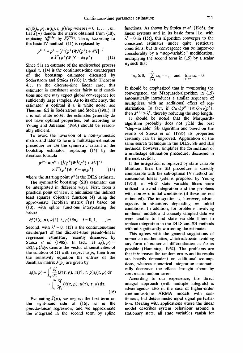
ILS estimators are given in Table 1, together with the estimates reported by the original authors. For all these estimates, it has been assumed that R = 02I. It may be seen from Table 1 that the performance of the three methods is comparable, in spite of the relatively large standard deviations of the estimates. The residual sum of errors is only slightly decreased in the SB and ILS stages. Figure 1 shows the fit only for the ILS estimator, since the response
TABLE 1. ESTIMATES IN EXAMPLE 1 FROM PUBLISHED DATA
Parameter p• P2 P3 Objective function
Starting value 0.22000 3.2700 24.440 DILS 0.24758 5.5848 24.390
SB 0.24550 5.3549 24.391 ILS 0.24644 5.4259 24.395 Reported by 0.24647 5.4290 24.395
Uno et al. (1979)
St. deviation 0.02922 2.0026 0.394 reported by authors
1~o. 1. Response functions in Example 1 fitted by the ILS me thod to published data indicated by symbols Is.
functions obtained in the different stages are practically indistinguishable.
Conditions (a)-(c) of Section 5 are all satisfied. The eigenvalues for the DILS es- timator, 6.32x 10 3, 3.56x 10² and 1.47 are greater than those in the ILS method, 3.49 x 10 3, 2.76x 10² and 1.38, but the differences are considerably less than an order of magnitude, so that, for the simulated data, we would expect neither significantly improved mean-squared errors nor significantly less variance than in the DILS stage.
The additional data sets have 5% and 10% relative errors added to the model response values (i.e. the standard deviation of the normally distributed errors is 5% or 10% of each response value). The results from the five runs are summarized in Table 2; for all runs, unweighted least squares was used. For both noise levels, the two methods are comparable, as expected, with ILS being slightly worse than DILS, in terms of both L 2 and L z. The
TABLE 2. SIMULATION RESULTS IN EXAMPLE 1
% Error Statistics DILS SB ILS
L 2 • 4.715 4.546 4.896 5 L 2 5.276 5.115 5.444
L 21 15.818 13.435 17.983 10
L22 28.860 26.063 33.514
714 S. VAJDA et al.
symmetric bootstrap (SB) method is slightly better than both DILS and ILS.
We note that the physical sources of poor conditioning have been recently discussed for models similar to the one considered here (Tong and Metzler, 1980; Godfrey and Fitch, 1984). In our case the eigenvector corresponding to the smallest eigenvalue ,~min of JT(fl)WJ(fl) shows that P2 is estimated with large variance, as confirmed by the last row of Table 1. In fact, except at the three last observations P2 < x and the value of P2 only weakly influences the response function. Further observations with decreasing x might improve the situation, but these usually lead to small signal-to-noise ratio. While poor conditioning may be somewhat improved also by continuous input perturba- tions, such experiments are usually very difficult to perform in drug kinetics studies.
Example 2. DILS much better than ILS The data are from a model for the
hydrogenation of fatty oils in a catalytic reactor (Yermakova and Umbetov, 1980):
Xl = P 6 ( P l + p 2 ) x l / g
YC2 = p 6 [ p I X , - - (P3 + p 4 ) x 2 + 1 . 5 p 3 x 3 ] / g
x3 =P6[pzxl +p3x2 - (1.5p3 + ps)x3]/g
where g=p6+(pl+p2)xl+p4x2+psx3. The data set is from a zero-input experiment with initial conditions x0 = [1 000] T and is given by Vajda et al. (1986).
Parameter estimates using the three methods are given in Table 3, in all cases, it has been assumed that R = o2L Response functions fitted in different stages of the procedure are indistinguishable and are shown in Fig. 2.
Conditions (a)-(c) of Section 5 are again all satisfied, but unlike Example 1, SzLs >> SDms, the eigenvalues for the DILS estimator being 6.6, 4.0, 2.3, 0.15, 2 .9x 10 -2 and 1.1 x 10 -3 and those for the ILS estimator being 1.2, 0.27, 0.26, 2.2 x 10 -2 , 1.6 x 10 -2 and 2.6 x 10 -4 . Thus we expect that, for the simulated data, the DILS
estimates will be significantly better than the ILS estimates, in terms of both L~ and Lz 2.
This is confirmed in Table 4, which sum- marizes results from additional data sets with 5% and 10% relative errors added to the model response values. We also note from Table 4 that the SB estimates are much better than the ILS estimates, but are not as good as the DILS estimates.
Example 3. ILS estimator increases variance but decreases mean-squared error
The data are from test problem 3 of a model of chemical reaction kinetics (Bard, 1970) described by
kl = -p lxxx2 + p2x3
fC2 = - - p l X 1 X 2 + p 2 X 3 - - p 4 X 2 X 3 + PsX5 - p 6 x 2 x 4
.ic 3 = p l X l X 2 - p 2 x 3 - p 3 x 3 - p 4 x 2 x 3
fc4 = p 3 x 3 + psx5 - p 6 x 2 x 4
.if 5 = p 4 x 2 x 3 - p s x 5 + p 6 x 2 x 4 .
The data set consists of eight sample points from a zero-input experiment with x0 = [1 1 0 0 0] r.
The results from the three methods, and those of Bard (1970) are given in Table 5. The disturbances are assumed to be uncorrelated and for each sample point, the covariance matrix is R = 25 x 1 0 - S w -1 where W - l = d i a g
TABLE 3. ESTIMATES IN EXAMPLE 2 FROM PUBLISHED DATA
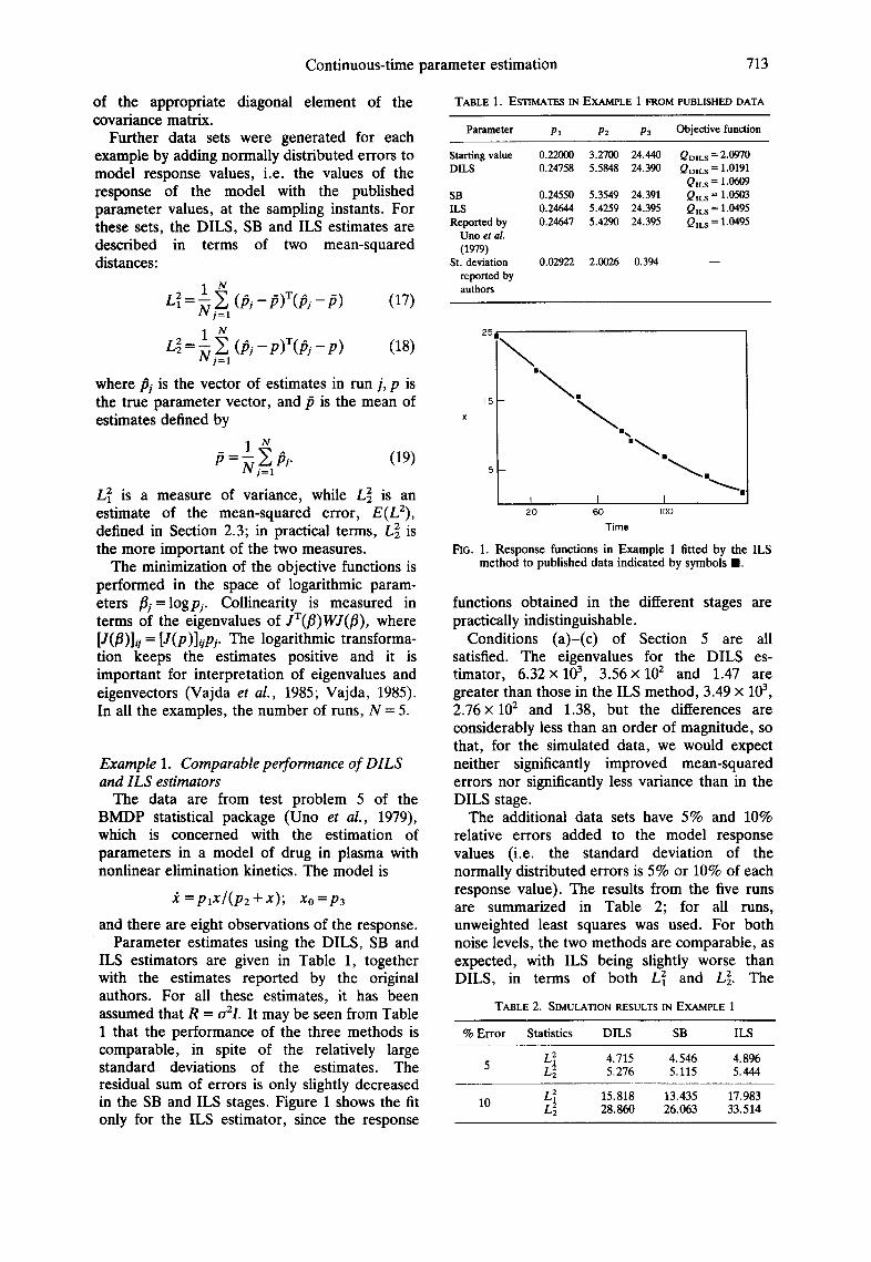
[100100 1 10 -2 10-4]; the Ws are used as weighting matrices of the observations. It may be seen from Table 5 that the three methods yield rather different estimates, though the DILS estimates are contained in the 95% confidence intervals of the estimates given by Bard. Even using rather more iterations in the ILS stage than Bard (15 compared with 12), we were unable to obtain quite as low a minimum. In spite of different parameter values, however, the response functions derived in the three stages are very close and hence are shown only for the ILS method in Fig. 3.
The eigenvalues for the DILS estimator are 1.54, 6.33 x 10 -1, 3.51 × 10 -3, 2.28 × 10 -3, 8.68 X 10 -6 and 1.19 × 10 -7, while those for the ILS estimator are 7 .28x10 -2, 1 .23x10 -2, 1.41 x 10 -3, 5.84 X 10 -4, 2.03 x 10 -6 and 2.85 x 10 -7. In this case, conditions (a) and (b) of Section 5 are satisfied, but condition (c) is not and we therefore expect that for the simulated data runs, the ILS method will increase L 2 but decrease L 2. This is confirmed in Table 6, which summarizes simulation results from noisy data with the covariance matrix R as assumed by Bard and given above. The SB estimator almost attains the L 2 value of the ILS estimator.
Example 4. Poor prediction using spline functions
The model in this example is of a microbial growth process (Nihtil/i and Virkkunen, 1977; Holmberg and Ranta, 1982) described by
pl(x2 -Ps)Xl Xl = p 3 X l ; X l ( 0 ) = p 6
P 2 + X2 -- P 5
1 pl(xz-ps)xl "~2 = - - - - ; x2(O) = P 7 + P 5
P 4 P 2 + X2 - - P 5
, r ~ . ~ o _ ,~ 0 - C M o [
V / I 0 30 50 70 90
Time
FIG. 3. R e s p o n s e func t ions in E x a m p l e 3 f i t ted by ILS m e t h o d to the p u b l i s h e d d a t a d e n o t e d by the fo l lowing symbols : [2yx; (Dy2, • 10(y3); /k 102(y4); O103(y5) . No t i ce tha t yx and Y2 a lmos t co inc ide and hence Y2 is p lo t t ed by a
where P5 represents the constant bias in x 2. Parameters are estimated from 16 samples from a zero-input experiment.
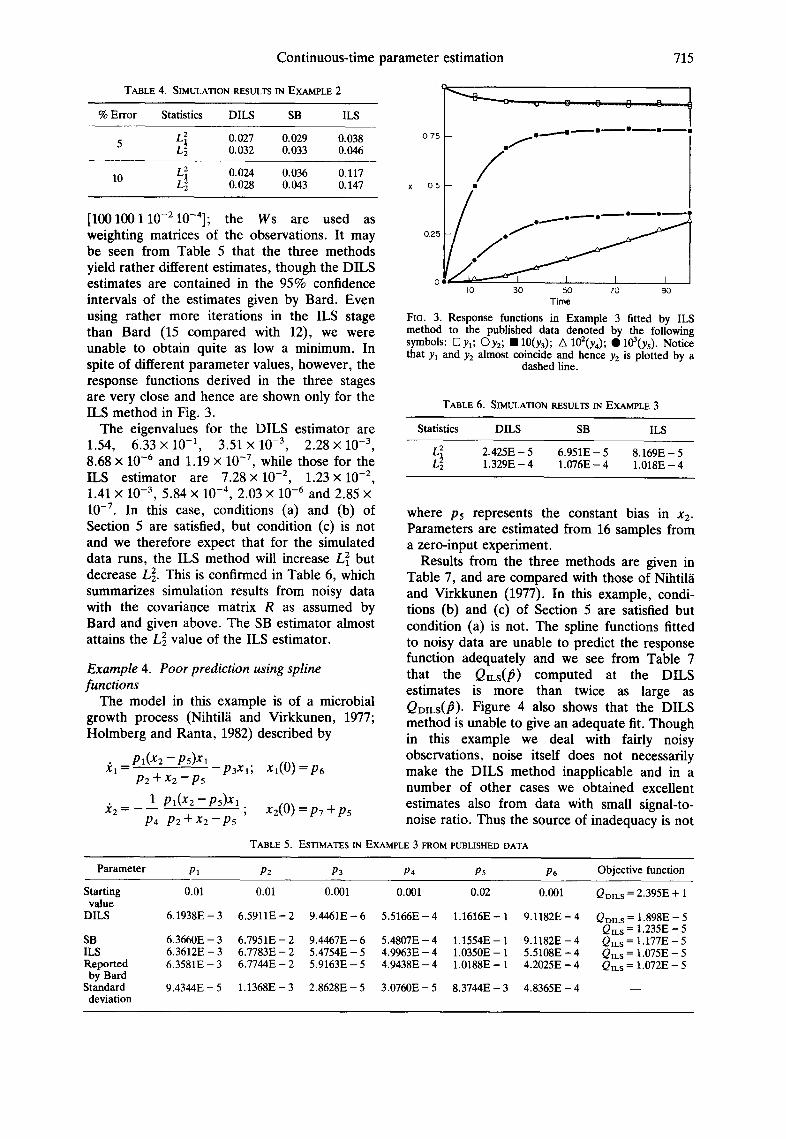
Results from the three methods are given in Table 7, and are compared with those of Nihtil~i and Virkkunen (1977). In this example, condi- tions (b) and (c) of Section 5 are satisfied but condition (a) is not. The spline functions fitted to noisy data are unable to predict the response function adequately and we see from Table 7 that the Q~LS(/)) computed at the DILS estimates is more than twice as large as QDILS(/~). Figure 4 also shows that the DILS method is unable to give an adequate fit. Though in this example we deal with fairly noisy observations, noise itself does not necessarily make the DILS method inapplicable and in a number of other cases we obtained excellent estimates also from data with small signal-to- noise ratio. Thus the source of inadequacy is not
TABLE 5. ESTIMATES IN EXAMPLE 3 FROM PUBLISHED DATA
P a r a m e t e r Pa P2 P3 P4 P5 P6 O b j e c t i v e func t ion
S ta r t ing 0.01 0.01 0.001 0.001 0.02 0.001 QDILS = 2 .395E + 1 va lue
D I L S 6 .1938E - 3 6 .5911E - 2 9 .4461E - 6 5 .5166E - 4 1 .1616E - 1 9 .1182E - 4 QDILS = 1.898E - 5 Q m s = 1.235E - 5
FIG. 4. Response function in Example 4 fitted by ILS and DILS methods to published data: • Yl; [] Y2.
completely understood, but the situation can easily be detected by checking condition (a).
The additional data sets in this example are obtained with absolute errors with standard deviations of 0.2 and 0.6. This corresponds with additional data sets generated by Nihtil~i and Virkkunen (1977). The results presented in Table 8 confirm that, using spline predictions, the DILS estimator performs very poorly and even the SB stage is unable to remove biasedness, since the approximate Jacobian J(p) is also poor.
The problem is avoided by using piecewise linear interpolation instead of splines, as illustrated also in Table 8. For the data with standard deviation of 0.2, the DILS method gives the best estimates, while for the standard deviation of 0.6, the SB estimator is better than either the DILS or ILS estimators.
Apart from the difficulty with the spline predictions, this example is quite similar to Example 1, with similar eigenvalues for the DILS and ILS estimators.
6.1. Computational effort The computational effort required for estimat-
ing the parameters of the published sets of data in Examples 1-4 is summarized in Table 9.
TABLE 8. SIMULATION RESULTS IN EXAMPLE 4
Interpolation SD Statistics DILS SB ILS
L~ 1.712 1.595 1.584 0.2 2
L 2 4.426 3.922 2.754 Spline
L~ 182.70 179.48 3.989 0.6 L2 z 300.49 290.59 4.121
L 2 0.928 1.391 1.584 Linear 0.2 z L 2 0.960 1.539 2.754 (Trapezium method) 0.6 L~ 5.046 3.841 3.989
L 2 5.434 3.932 4.121
TABLE 9. COMPARISON OF COMPUTATIONAL EffORT
Number of Number of equivalent iterations function evaluations
For all cases, the termination condition was [pk+l _pkl/pk< 1 0 - 4 and the number of itera- tions was restricted to 15.
The left half of the table shows the number of iterations in the separate steps of the multistage procedure. Example 3 involves a model linear in the parameters, so that the DILS estimates could, in principle, be obtained in a single iteration, but, gradually decreasing the param- eter zk, the Marquardt algorithm requires a few steps to attain the termination condition. The number of iterations in the SB stage can also be considered as an indicator for the applicability of the DILS method. In Example 1, where the method is expected to perform as well as the ILS estimator, the SB method converges in three steps, thereby slightly reducing both L 2 and L g, as shown in Table 2. In Example 2, the DILS estimator is definitely preferable. Using the published data, the SB stage is terminated in the
Continuous-time parameter estimation 717
first iteration and the estimates are unchanged as shown in Table 3. In some simulation runs for the same example, up to three steps have been taken.
The maximum allowed number of iterations has been performed both in Example 3, where the DILS method is not preferable, and in Example 4, where the method is not suitable. When piecewise linear interpolation has been used instead of splines in Example 4, the number of iterations was reduced.
The columns in the right-hand part of Table 9 show the number of equivalent function evaluations successively in the DILS and SB stages, in all three stages and in solving the problem by the ILS method on its own. Using only the first two stages, the number of equivalent function evaluations equals the number of iterations in the SB stage. From our results, the SB estimates were quite satisfactory in all examples and comparison with the last column of Table 9 emphasizes the numerical efficiency of the direct approach involving the DILS and SB estimators. We note that the convergence of the SB algorithm is relatively slow. As emphasized in Section 2.3, our aim is, however, not attaining the minimum of QILS (frequently resulting in large variance and mean-squared error of the estimates), but a reasonable compromise between the DILS and ILS methods, reducing the bias while avoiding consequences of near-collinearity. According to the simulation studies presented here, a few steps of the SB algorithm serves this purpose efficiently.
7. CONCLUSIONS
Well-established discrete-time parameter es- timation techniques have been extended to continuous-time, nonlinear models and it has been shown that, in most cases, the direct integral least squares (DILS) and symmetric bootstrap (SB) estimators are numerically efficient and are statistically sound alternatives to the conventional indirect least squares (ILS) approach. The simple DILS method is pre- ferable, in terms of mean-squared error of the estimates, to the more involved ILS method in nearly-singular estimation problems, frequently encountered in applications with physically justified models. On the other hand, widely separated sample points and/or a low signal-to- noise ratio may render the spline prediction unacceptable in the DILS method, resulting in very biased estimates. In view of this trade-off between biasedness and mean-squared error, the SB estimator is usually advantageous, despite its slow convergence, since it reduces the biasedness
of the DILS estimates while keeping the mean-squared error small.
The estimators form a three-stage estimation procedure. By inspecting simple statistics evalu- ated at DILS parameter estimates, namely the residual sum of squares with and without spline prediction of the response and eigenvalues of the approximate Hessian matrices in the DILS and ILS method, it is possible to decide whether the DILS estimates are satisfactory or if it is necessary to proceed to the more involved SB and ILS stages.
In most applications, a few iterations of the SB algorithm, started at the DILS estimates, yields results at least as good as the computa- tionally more expensive ILS method. Thus the direct approach often results in a considerable saving of computational effort.
REFERENCES
,~str6m, K. J. and P. Eykhoff (1971). System identification-- a survey. Automatica, 7, 123.
Bard, Y. (1970). Comparison of gradient methods for the solution of nonlinear parameter estimation problems. SIAM J. Numer. Anal., 7, 157.
Bard, Y. (1974). Nonlinear Parameter Estimation. Academic Press, New York.
Bates, D. M. and D. G. Watts (1985). Multiresponse estimation with special application to linear systems of differential equations. Technometrics, 27, 329.
Cobelli, C. (1985). Identification of endocrine-metabolic and pharmacokinetic systems. In Barker, H. A. and P. C. Young (Eds), Identification and System Parameter Estimation, Vol. 1, pp. 45-54 (7th IFAC/IFORS Symp.). Pergamon, Oxford.
Endrenyi, L. (Ed.) (1981) Kinetic Data Analysis. Plenum, New York.
Gelinas, R. J. (1972). Stiff systems of kinetic equations---a practitioner's view. J. Comput. Phys., 9, 222.
Gevers, M. and A. C. Tsoi (1984). Structural identification of linear multivariable systems using overlapping forms: a new parametrization. Int. J. Control, 40, 971.
Godfrey, K. R. and W. R. Fitch (1984). On the identification of Michaelis-Menten elimination parameters from a single dose-response curve. J. Pharmocokin. Biopharm., 12, 193.
Goodwin, G. C. and R. L. Payne (1977). Dynamic System Identification: Experiment Design and Data Analysis. Academic Press, New York.
Hamming, R. W. (1962). Numerical Methods for Scientists and Engineers. McGraw-Hill, New York.
Himmelblau, D. M. (1970). Process Analysis by Statistical Methods. Wiley, New York.
Himmelblau, D. M., C. R. Jones and K. B. Bischoff (1967). Determination of rate constants for complex kinetic models. Ind. Eng. Chem. Fund., 6, 539.
Hocking, R. R. (1983). Developments in linear regression methodology: 1959-1982. Technometrics, 25, 219.
Hoerl, A. E. and R. W. Kennard (1970). Ridge regression: biased estimation for non-orthogonal problems. Technometrics, 12, 55.
Holmberg, A. and J. Ranta (1982). Procedures for parameter and state estimation of microbial growth process models. Automatica, 18, 181-193.
Hosten, L. H. (1979). A comparative study of short cut procedures for parameter estimation in differential equations. Comput. Chem. Engng., 3, 117.
Jennrich, R. I. (1969). Asymptotic properties of non-linear least squares estimators. Ann. Math. Statist, 40, 633.
718 S. VAJDA et al.
Jennrich, R. I. and P. F. Sampson (1968). Application of stepwise regression to non-linear estimation. Technometrics, 10, 63.
Joseph, P., J. Lewis and J. Tou (1961). Plant identification in the presence of disturbances and application to digital adaptive systems. AIEE Trans. App. Ind., 80, 18.
Klonowski, W. (1983). Simplifying principles for chemical and enzyme reaction kinetics. Biophys. Chem., 18, 73.
Loeb, J. H. and G. M. Cahen (1965). More about process identification. IEEE Trans. Aut. Control, AC-10, 359.
Mori, F. and J. J. DiStefano, III. (1979). Optimal nonuniform sampling interval and test-input design for identification of physiological systems from very limited data. IEEE Trans. Aut. Control, AC-24, 893.
Nazareth, L. (1980). Some recent approaches to solving large residual nonlinear least squares problems. SlAM Rev., 22, 1.
Nihtila, M. and J. Virkkunen (1977). Practical identifiability of growth and substrate consumption models. Biotech. Bioengng, 19, 1831.
Sinha, N. K. and Z. Qijie (1985). Identification of continuous-time systems from sampled data: a comparison of 3 direct methods. In Barker, H. A. and P. C. Young (Eds.), Identification and System Parameter Estimation, Vol. 1, pp. 1575-1578 (7th IFAC/IFORS Symp.). Pergamon, Oxford.
S6derstr6m, T. and P. Stoica (1981). Comparison of some instrumental variable methods--consistency and accuracy aspects. Automatica, 17, 101-115.
S6derstr6m, T. and P. G. Stoica (1983). Instrumental Variable Methods for System Identification. Springer, Berlin.
Sorenson, H. W. (1980). Parameter Estimation--Principles and Problems. Marcel Dekker, New York.
Stoica, P., T. S6derstr6m, A. Ahlen and G. Soibrand (1985). On the convergence of pseudo-linear regression algo- rithms. Int. J. Control, 41, 1429.
Strejc, V. (1980). Least squares parameter estimation. Automatica, 16, 535-550.
Tong, D. D. M. and C. M. Metzler (1980). Mathematical properties of compartment models with Michaelis-Menten type elimination. Math. Biosci., 48, 293.
Uno, F. K., M. L. Ralston, R. I. Jennrich and P. F. Sampson (1979). Test problems from the pharmacokinetic literature requiring fitting models defined by differential equations. Tech. Report No. 61, BMDP. Statistical Software, Department of Biomathematics, University of California, Los Angeles.
Vajda, S. (1985). Identifiability of polynomial and rational systems: structural and numerical aspects. In Barker, H. A. and P. C. Young (Eds.), Identification and System Parameter Estimation, Vol. 1, pp. 537-542 (7th IFAC/IFORS Symp.). Pergamon, Oxford.
Vajda, S., P. Valko and T. Turanyi (1985). Principal component analysis of kinetic models. Int. J. Chem. Kinet., 17, 55.
Vajda, S., P. Valko and A. Yermakova (1986). A direct-indirect procedure for estimating kinetic param- eters. Comput. Chem. Engng., 10, 49.
Wong, K. Y. and E. Polak (1967). Identification of linear discrete time systems using the instrumental variable approach. IEEE Trans. Aut. Control, AC-12, 707.
Yermakova, A. and A. S. Umbetov (1980). Diffusion kinetics of selective hydrogenation of fatty oils in a stationary catalyst bed reactor. Reactor Kinet. Catal. Lett., 14, 187.
Yermakova, A., S. Vajda and P. Valko (1982). Direct integral method via spline approximation for estimating rate constants. Appl. Catal., 2, 139.
Young, P. C. (1970). An instrumental variable method for real time identification of a noisy process. Automatica, 6, 271.
Young, P. C. (1981). Parameter estimation for continuous- time models--a survey. Automatica, 17, 23-39.
Young, P. C. and A. Jakeman (1980). Refined instrumental variable methods of recursive time-series analysis, Part III. Extensions. Int. J. Control, 31, 741.