Direct correlation of 4D seismic with well activity for a ...

Geophysical Prospecting, 2012, 60, 293–312 doi: 10.1111/j.1365-2478.2011.00995.x

Direct correlation of 4D seismic with well activity for a clarifieddynamic reservoir interpretation

Yi Huang and Colin MacBeth∗Institute of Petroleum Engineering, Heriot-Watt University, Riccarton, Edinburgh, EH14 4AS, UK

Received November 2010, revision accepted June 2011

ABSTRACTA method to provide an improved time-lapse seismic attribute for dynamic interpre-tation is presented. This is based on the causal link between the time-lapse seismicresponse and well production activity taken over time. The resultant image is ob-tained by computing correlation coefficients between sequences of time-lapse seismicchanges extracted over different time intervals from multiply repeated seismic andidentical time sequences of cumulative fluid volumes produced or injected from thewells. Maps of these cross-correlations show localized, spatially contiguous signalssurrounding individual wells or a specific well group. These may be associated withconnected regions around the selected well or well group. Application firstly to asynthetic data set reveals that hydraulic compartments may be delineated using thismethod. A second application to a field data set provides empirical evidence that aconnected well-centric fault block and active geobody can be detected. It is concludedthat uniting well data and time-lapse seismic using our proposed method delivers anew attribute for dynamic interpretation and potential updating of the model for theproducing reservoir.

Key words: 4D seismics, Stable state, Well activity.

INTRODUCTIO N

Despite the efforts made to process observed 4D seismic data itis not yet possible to carry out a quantitative interpretation fordynamic reservoir characterization. Indeed, inversions of 4Dseismic to pressure and saturation changes (Tura and Lumley1999; Landrø 2001; MacBeth, Floricich and Soldo 2006) re-vealed that inconsistencies still exist between the time-lapsedseismic and the engineering domains. Furthermore, the proce-dure of seismic history matching, which relies upon simulator-to seismic modelling, continues to reveal some degree ofmismatch between observed and predicted time-lapse seismicdata and as a consequence many studies are based mainly ona visual comparison (Stephen and MacBeth 2006). One possi-ble key to bridging these two domains is the recognition that

∗E-mail: [email protected]

the 4D seismic signatures must respond directly to changes inwell production and injection occurring over the time periodsin which the 4D surveys are shot. A calibration of this naturewas first considered by Huang, Will and Waggoner (2000)who used material balance and known well data to thresholdseismic amplitudes for the estimation of gas volume distri-bution. Here, this concept is extended and it will be shownthat time-lapse seismic data can be correlated directly to thewell activity over production time. More specifically, integrat-ing the changes in well volumes between seismic survey datesallows us to focus only on the part of the seismic signatureresponding to dynamic reservoir change.

To implement the above understanding requires multipleseismic surveys shot at frequent intervals over the same reser-voir. Fortunately, there are now many fields in the NorthSea for which such data sets have become available. For ex-ample, Life of Field Seismic projects were implemented onthe Valhall field (Barkved et al. 2006), which have so far

C© 2011 European Association of Geoscientists & Engineers 293

294 Y. Huang and C. MacBeth

delivered twelve 3D seismic surveys shot at a time intervalof 2–10 months. Similar projects were implemented on theClair field (Foster et al. 2008), the Snorre field (Morton, An-dersen and Thompson 2009) and the Ekofisk field (Haug-valdstad et al. 2010). In the wider context, many fields suchas Norne (Osdal and Alsos 2010) and Schiehallion (Floricichet al. 2008) were repeatedly shot with seven or eight towedstreamer surveys at intervals of 12–24 months apart. Further-more, the potential of multiple repeated surveys is now be-ginning to be recognized. For example, Floricich et al. (2008)overlapped trace-to-trace coherence from multiple surveys forenhanced barrier interpretation in the Schiehallion field. Webelieve that frequent monitoring also opens up the possibil-ity of interpreting how the 4D seismic signal evolves overtime and may reveal many future benefits for dynamic reser-voir characterization, including permeability estimation andpressure-saturation change separation. Unifying seismic andwell rate history on a common time-scale aids quantitativeintegration between the softer (non-unique) seismic productwith good areal coverage and the harder (unique) spatiallysparse well data. In this current publication we develop themethodology for such a technique when applied to data forwhich the seismic signatures are predominantly sensitive topressure. A companion paper, Huang et al. (2011), providesanother application of this technique to pressure and satura-tion sensitive seismic attributes.

METHOD

Development of the link between cumulative well volumesand the 4D seismic signatures

Consider a non-compacting reservoir in which only oil andwater are present. The 4D seismic signature is driven solelyby changes in the pressure and water saturation induced bythe production and injection activity. These changes are, inturn, dependent on the net cumulative volume �V of the pro-duced or injected fluids from each well and their fluctuationsover time. Thus, it is natural to assume that at any particularlocation in the reservoir, the time-lapse change of a mappedseismic attribute �A is a correlatable function of the reser-voir’s well activity. Indeed, to link cause (seismic) with effect(wells), the pressure-saturation change equation proposed byMacBeth et al. (2006) can be modified to explicitly involveonly well data (Huang and MacBeth 2009). Consider the spe-cific case of a pressure-controlled 4D seismic signature forwhich the contribution from saturation changes is suppressedrelative to the pressure – from our experience to date, in clastic

and chalk reservoirs identification of the pressure signal ap-pears possible in most cases. In this case, at any (x,y) locationon the reservoir

�A(x, y) = H(x, y)�P(x, y), (1)

where the coefficient H(x, y)is related to the local geology,fluids and the flow boundary conditions. This linear equationis shown to be valid for pressure changes of up to ±5 MPa(Floricich 2006). It is also known that the pressure changein every compartment of the reservoir is determined by thesuperposition of contributions from each well in, or connectedto, this compartment. In the kth time interval �Tk between twoparticular seismic surveys, pressure can be assumed to be ina stable state (the limits of this assumption will be discussedin a later section). Under this condition, the pressure changeresulting from M injectors and N producers is

�Pk = 1ctV

⎛⎝Bw

M∑i=1

�Vwik + Bo

N∑j=1

�Vojk + Bw

N∑l=1

�Vwlk

⎞⎠ ,

(2)

where ct is the total rock and fluid compressibility of the se-lected compartment, V its total volume and Bw and Bo thewater and oil formation volume factors respectively. �V isdefined as being positive for water injection and negative foroil and water production. This equation is valid provided thebeginning or end of the seismic survey period �Tk does notcoincide with transients associated with major well start-ups,shut downs or rate changes (see the Appendix for details).Furthermore, equation (2) is valid regardless of the well po-sitions, the geometry of the compartment or nature of theexternal boundary conditions. However, the group of wellsthat contribute to any selected pressure compartment is usu-ally largely unknown, as it depends on the degree of internalconnectivity and inter-compartment communication for thefield. This point is further discussed in the model example inthe next section. Combining equations (1) and (2) connectsthe 4D seismic signature to the net cumulative fluid volumesfrom the wells.

The above concept can be utilized effectively if data ac-quired from multiple repeated surveys are available. If manyvintages of the survey are shot over the same reservoir com-partment at different time intervals �Tk (k = 1 to P), it ispossible to form a sequence of 4D signatures {�Ak = �A(x,

y, �Tk), k = 1,P} at each location (x,y) associated with asimilarly derived sequence of net cumulative formation vol-umes {�Vk = �V(�Tk), k = 1,P} derived from integrat-ing the well surface volume changes after weighting by the

C© 2011 European Association of Geoscientists & Engineers, Geophysical Prospecting, 60, 293–312

Direct correlation of 4D seismic with well activity 295

formation volume factors as in the right-hand side of equation(2). Combining equations (1) and (2) for each time interval�Tk (k = 1 to P), the amplitudes are given by

�Ak(x, y, �Tk) = H(x, y)ctV

�Vk. (3)

The sequence of seismic amplitudes is therefore linearly cor-related with the net cumulative well volume sequence. Inpractice, the normalized cross-correlation coefficient (NCC)

is formed between the time sequence vector of 4D seismic sig-natures (�A1, �A2, �A3, . . . . . . �AP ) and that correspondingto the net well activity (�V1, �V2, �V3, . . . . . . �VP ), thus pro-viding a measure of the similarity between these two data sets

NCC

=

P∑k=1

(�Ak − �A)(�Vk − �V)

√√√√ P∑k=1

(�Ak − �A)(�Ak − �A)

√√√√ P∑k=1

(�Vk − �V)(�Vk − �V)

.

(4)

This metric is equal to 1 for perfect correlation and between0–1 if noise is present (or if the observed data does not con-form with the above predictions). The coefficient NCC is cal-culated for each seismic bin, thus producing a map of thecompartment or reservoir region of interest and providing adescriptive measure of the degree of connectivity to the wellsof interest.

Modelled example

We now evaluate the validity of the above prediction by con-sidering numerical models of a simple idealized reservoir con-sisting of two compartments separated by a sealing and apartially sealing fault (Fig. 1). Model properties and dimen-sions are chosen to be typical of channelized turbidites in theNorth Sea (Leach et al. 1999). The fault separating the com-partments is assumed to be unforeseen during interpretation.Three flow simulations evaluate the consequences of possibleleakage across the fault. In the left-hand compartment, thereare two injectors I1 and I2 and one producer P1 and in theright-hand compartment there is one injector I3. The injectorsand producer are activated according to what might be ex-pected for a typical reservoir (Fig. 2). The sequence is chosento give net total surface volumes for I1, I2, I3 and P1, whichbalance close to zero at any particular time. The first monitorseismic survey (R1) is shot after 12 months of production,thereafter additional monitor surveys (R2, R3, . . .) are shotevery 18 months.

Figure 1 The three flow simulation models used to test our methodof net well volume to pressure correlation taken over repeated seis-mic time intervals. The model properties are based loosely on theSchiehallion field, North Sea: porosity of 28%, ct = 2.210−5psi−1

and permeability of 280 mD. a) Model 1 – sealed compartments; b)Model 2 – partially sealing fault with fault transmissibility of 0.005;c) Model 3 – partially sealing fault with fault transmissibility of 0.01.Dimensions are 1200 m × 900 m for the left-hand compartment and1200 m × 300 m for the right-hand one.



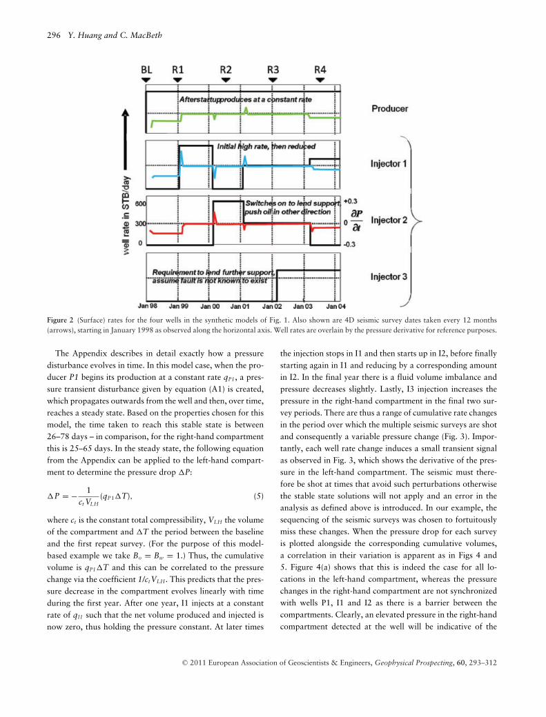
Figure 2 (Surface) rates for the four wells in the synthetic models of Fig. 1. Also shown are 4D seismic survey dates taken every 12 months(arrows), starting in January 1998 as observed along the horizontal axis. Well rates are overlain by the pressure derivative for reference purposes.

The Appendix describes in detail exactly how a pressuredisturbance evolves in time. In this model case, when the pro-ducer P1 begins its production at a constant rate qP1, a pres-sure transient disturbance given by equation (A1) is created,which propagates outwards from the well and then, over time,reaches a steady state. Based on the properties chosen for thismodel, the time taken to reach this stable state is between26–78 days – in comparison, for the right-hand compartmentthis is 25–65 days. In the steady state, the following equationfrom the Appendix can be applied to the left-hand compart-ment to determine the pressure drop �P:

�P = − 1ctVLH

(qP1�T), (5)

where ct is the constant total compressibility, VLH the volumeof the compartment and �T the period between the baselineand the first repeat survey. (For the purpose of this model-based example we take Bo = Bw = 1.) Thus, the cumulativevolume is qP1�T and this can be correlated to the pressurechange via the coefficient 1/ctVLH. This predicts that the pres-sure decrease in the compartment evolves linearly with timeduring the first year. After one year, I1 injects at a constantrate of qI1 such that the net volume produced and injected isnow zero, thus holding the pressure constant. At later times

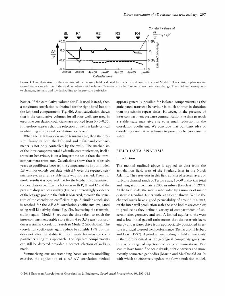
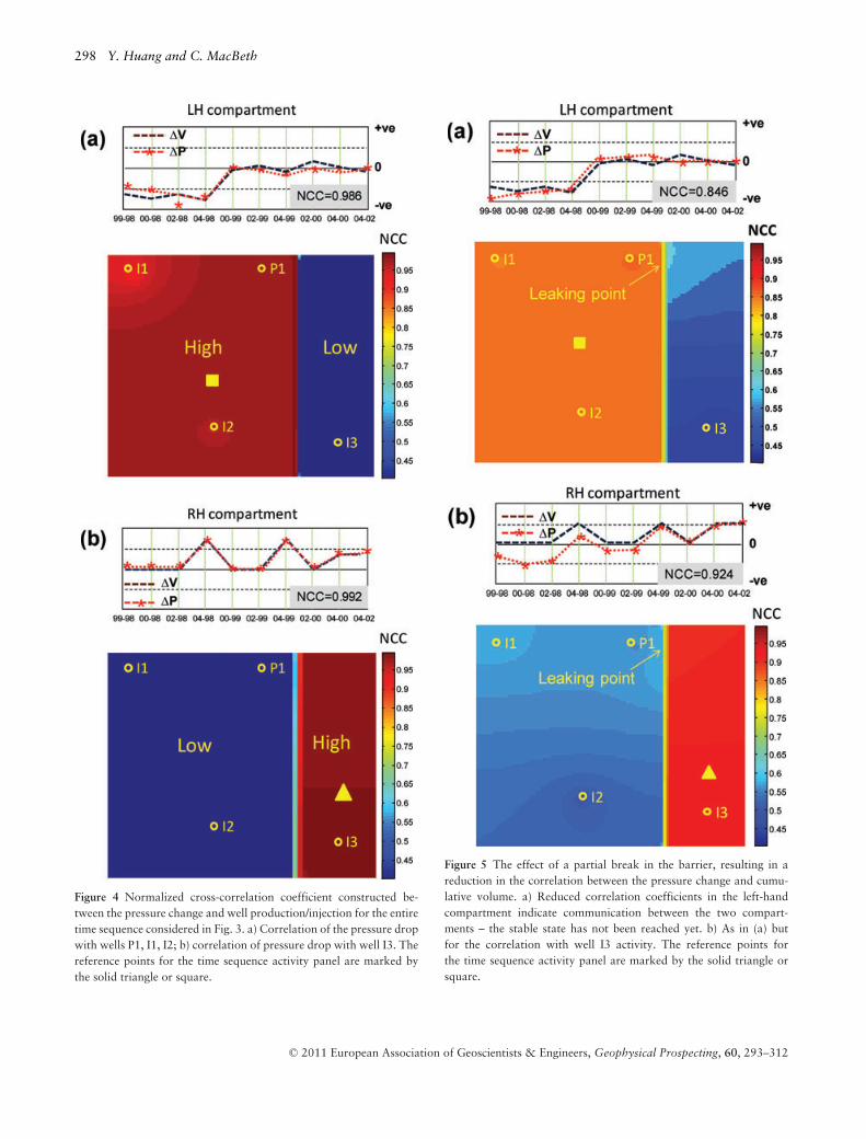
the injection stops in I1 and then starts up in I2, before finallystarting again in I1 and reducing by a corresponding amountin I2. In the final year there is a fluid volume imbalance andpressure decreases slightly. Lastly, I3 injection increases thepressure in the right-hand compartment in the final two sur-vey periods. There are thus a range of cumulative rate changesin the period over which the multiple seismic surveys are shotand consequently a variable pressure change (Fig. 3). Impor-tantly, each well rate change induces a small transient signalas observed in Fig. 3, which shows the derivative of the pres-sure in the left-hand compartment. The seismic must there-fore be shot at times that avoid such perturbations otherwisethe stable state solutions will not apply and an error in theanalysis as defined above is introduced. In our example, thesequencing of the seismic surveys was chosen to fortuitouslymiss these changes. When the pressure drop for each surveyis plotted alongside the corresponding cumulative volumes,a correlation in their variation is apparent as in Figs 4 and5. Figure 4(a) shows that this is indeed the case for all lo-cations in the left-hand compartment, whereas the pressurechanges in the right-hand compartment are not synchronizedwith wells P1, I1 and I2 as there is a barrier between thecompartments. Clearly, an elevated pressure in the right-handcompartment detected at the well will be indicative of the



Figure 3 Time derivative for the evolution of the pressure field evaluated for the left-hand compartment of Model 1. The constant plateaus arerelated to the cancellation of the total cumulative well volumes. Transients can be observed at each well rate change. The solid line correspondsto changing pressure and the dashed line to the pressure derivative.

barrier. If the cumulative volume for I3 is used instead, thena maximum correlation is obtained for the right-hand but notthe left-hand compartment (Fig. 4b). Also, calculation showsthat if the cumulative volumes for all four wells are used inerror, the correlation coefficients are reduced from 0.90–0.55.It therefore appears that the selection of wells is fairly criticalin obtaining an optimal correlation coefficient.

When the fault barrier is made transmissible, then the pres-sure change in both the left-hand and right-hand compart-ments is not only controlled by the wells. The mechanismof the inter-compartmental hydraulic communication, itself atransient behaviour, is on a longer time scale than the intra-compartment transients. Calculations show that it takes sixyears to equilibrate between the compartments in our model.�P will not exactly correlate with �V over the repeated seis-mic surveys, as a fully stable state was not reached. From ourmodel results it is observed that for the left-hand compartmentthe correlation coefficients between wells P, I1 and I2 and thepressure drop reduces slightly (Fig. 5a). Interestingly, evidenceof the leakage point in the fault is observed, through the struc-ture of the correlation coefficient map. A similar conclusionis reached for the �P-�V correlation coefficients evaluatedusing well I3 activity alone (Fig. 5b). Increasing the transmis-sibility again (Model 3) reduces the time taken to reach theinter-compartment stable state (from 6 to 3.5 years) but pro-duces a similar correlation result to Model 2 (not shown). Thecorrelation coefficients again reduce by roughly 15% but thisdoes not alter the ability to discriminate between the com-partments using this approach. The separate compartmentscan still be detected provided a correct selection of wells ismade.

Summarizing our understanding based on this modellingexercise, the application of a �P-�V correlation method

appears generally possible for isolated compartments as theanticipated transient behaviour is much shorter in durationthan the seismic repeat times. However, in the presence ofinter-compartment pressure communication the time to reacha stable state may give rise to a small reduction in thecorrelation coefficient. We conclude that our basic idea ofcorrelating cumulative volumes to pressure changes remainsvalid.

F IELD DATA ANALYSIS

Introduction

The method outlined above is applied to data from theSchiehallion field, west of the Shetland Isles in the NorthAtlantic. The reservoirs in this field consist of several layers ofturbidite channel sands of Tertiary age, 10–50 m thick in totaland lying at approximately 2000 m subsea (Leach et al. 1999).At the field scale, the area is subdivided by a number of majoreast-west trending faults with significant throw. Whilst thechannel sands have a good permeability of around 600 mD,on the inter-well production scale the sand bodies are complexto produce as they define a variety of compartments of un-certain size, geometry and seal. A limited aquifer to the westand a low initial gas-oil ratio means that the reservoir lacksenergy and a water drive from appropriately positioned injec-tors is critical to good well performance (Richardson, Herbertand Leach 1997). A good understanding of field connectivityis therefore essential as the geological complexity gives riseto a wide range of injector-producer communications. Paststudies have found fine-scale details, subtle barriers and morerecently connected geobodies (Martin and MacDonald 2010)with which to effectively update the flow simulation model.



Figure 4 Normalized cross-correlation coefficient constructed be-tween the pressure change and well production/injection for the entiretime sequence considered in Fig. 3. a) Correlation of the pressure dropwith wells P1, I1, I2; b) correlation of pressure drop with well I3. Thereference points for the time sequence activity panel are marked bythe solid triangle or square.

Figure 5 The effect of a partial break in the barrier, resulting in areduction in the correlation between the pressure change and cumu-lative volume. a) Reduced correlation coefficients in the left-handcompartment indicate communication between the two compart-ments – the stable state has not been reached yet. b) As in (a) butfor the correlation with well I3 activity. The reference points forthe time sequence activity panel are marked by the solid triangle orsquare.



Such a setting is suited for the preliminary application of ourtechnique.

Our focus is on segment 4 in the south-eastern portion ofthe field, which lies between two major sealing faults. Fig-ure 6 shows five RMS amplitude attribute maps generatedfrom selected surveys over this segment. The 4D seismic dis-plays a softening of impedance at the injectors, consistent witha dominant pressure up response rather than a hardening fromwater invasion (Stephen and MacBeth 2006). Around some ofthe producers, gas out of solution creates a clear softening ef-fect – however these wells are not considered in the currentanalysis (for this reason we exclude the lower right area ofthe segment as we wish to concentrate only on the pressureeffects). Over most of the selected segment, the pressure sig-nal is the main control over the seismic amplitudes. For ourwork, we use the full stacked and migrated data, available for1996 (preproduction baseline), 1999, 2000, 2002 and 2004.These data have been cross-equalized and are of satisfactoryrepeatability (NRMS in the range 40–55%). For each survey,the RMS amplitude is mapped between the picked top andbase of the T31 interval. These five repeated seismic surveysgenerate in total ten mapped 4D signatures and these are ar-ranged as a time sequence for each spatial location. Well datafrom five producers and five injectors are also available todetermine the fluid volumes produced or injected over eachof the selected time intervals (Fig. 7). Not all of these wellsare active nor maintain constant rates for the full durationfrom production start-up until the last survey date. This vari-ation of well rates provides the diversity in the time sequencenecessary for the application of our method. To guide theanalysis, pressure and saturation changes corresponding tothe time sequences defined above are also extracted from theflow simulation model.

Initial qualitative inspection of the seismic data reveals areasonable correlation between the 4D seismic signatures andthe well activity. To ensure stability, a minimum thresholdvalue is needed for the NCC maps, as for a particular size oftime sequence the cross-correlation coefficient is statisticallysignificant only above a certain coefficient value. Below thisthreshold there is a chance that samples drawn at randomcan yield the same coefficient (Bevington 1975). For example,for the 10 points used here, sequences with correlation coef-ficients greater than 0.77 are significant at 99% confidence.Another reason for thresholding the NCC maps used in thecurrent work is to focus on the 4D signature induced only by aparticular well or group of wells and to exclude the contribu-tions from other wells. The correlation coefficient between theselected well group of interest and the seismic sequence must

in this case be higher than the sequence correlation betweenthe excluded wells and the selected group. We now select twoexamples from the segment to describe the resultant interpre-tation in detail.

Selected example 1 – water injector W3

Injector W3 is in the central north portion of segment 4 anddrilled to provide more support to the producers in the lo-cality (Fig. 8). At a sector level it was intended to supplypressure to P8 in the south and P9 in the east (outside the fig-ure perimeter). Unfortunately for oil production, W3 injectedinto a small isolated triangular fault block of roughly 1 km ×0.5 km, bounded along its northern edge by a major east-westsealing fault and along its remaining edges by smaller faultsor stratigraphic barriers. Transmissibility multipliers assignedto the simulation model along the block edges suggest that asmall amount of leakage to the west is anticipated. W3 be-came active just before May 2003 and injected at a relativelyconstant rate up to September 2005, beyond the time of thelast monitor survey in 2004. The well activity thus forms astep function in cumulative volume change between the 2002and 2004 surveys. The 4D seismic response shows a strongpressure up (softening) signal (Fig. 8a) and the prediction ofpressure change (2000 psi or 13.8 MPa) from the simulator(Fig. 9a) agrees with this response. Despite the magnitude ofthis predicted pressure increase being larger than the linearityassumption required for the seismic response, we will see be-low that a good cross-correlation signal can still be obtained.Figure 10(a) shows the time sequence of cumulative fluid vol-ume changes alongside the seismic RMS amplitude changes fortwo reference locations inside the fault block. The normalizedcross-correlations (NCC) are high and the known fault blockis readily delineated by mapping this attribute across the en-tire area. The mapped NCC attribute based on the predictedpressure changes from the simulator are also shown for visualcomparison only (Fig. 10b). This diagram validates the stronglinear correlation between the pressure change spread acrossthe entire fault block and the change in cumulative fluid vol-umes at well W3. It is the pressure change component of the4D signature (and hence the NCC attribute) that detects theboundaries of the fault block.

In contrast with the pressure, the water flood moving out-wards from W3 is confined to only a small region of approxi-mately 100 m in size around the injector (Fig. 10a,b). There isa visible drop in the NCC measure around the well observedin Fig. 10(a), which may have been caused by the effects ofsaturation. The shape of the saturation anomaly is controlled



Figure 6 The five seismic maps used to generate the time sequence for cross-correlation analysis. Maps are of normalized RMS amplitudederived from the coloured inversion product. Squares in the topmost diagram delineate study areas for the two selected examples described inthe text.



Figure 7 a) Instantaneous well productionand injection in normalized units (redrawnafter Edriz 2009); b) cumulative volume forthe wells of interest in our work.

by the net-to-gross variation within the block, whereas thespread in pressure change is unaffected by this heterogeneityand is defined instead by the transmissibility at the barriers.The net-to-gross variation is observed via the coloured inver-sion product mapped on the baseline seismic in Fig. 6. As thereis no imprint of the net-to-gross variation on the overall NCCmap, it is concluded that the observed result from Fig. 10(a)is controlled by pressure. The mapped NCC attribute indi-cates that the barriers inserted during history matching ofthe simulation model appear mostly consistent with the 4Dseismic. However, there are some points of discrepancy withthe simulator to the south and an extension of the signal inthis direction suggests a re-positioning of the barriers couldbe necessary. Secondly, to the west, there is a similar ex-tension of the signal, beyond that defined in the simulationmodel, suggesting another possible update to the barrier po-sition. Interestingly, incorporation of the P8 and P9 produced

volumes in the correlation calculation does not improve theresults – suggesting that any leakage points to outside thecompartment are on a larger time scale than the survey repeattimes.

Selected example 2 – producer P8

The horizontal well P8 produced, from September 2001, atan almost constant rate for the entire duration of the seis-mic surveys considered here. In its vicinity there are two in-jectors, W2 and W4 (Fig. 11). W4 started injecting in June2003 and was active at an almost constant rate after thatdate, whilst W2 was closed immediately after September 1999when it was found that it had been placed in an area withpoor connectivity. W2 was later re-activated at several fixedrates (see Fig. 7). In the simulation model this lack of connec-tivity is expressed as a north-south barrier (transmissibility



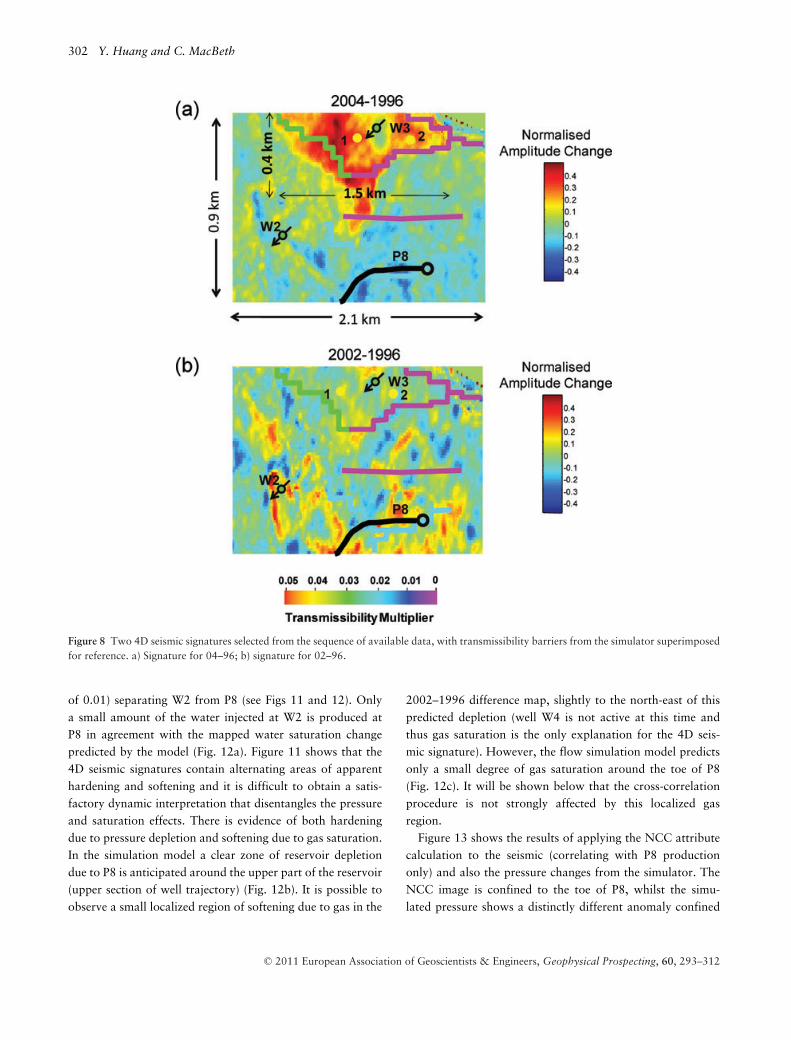
Figure 8 Two 4D seismic signatures selected from the sequence of available data, with transmissibility barriers from the simulator superimposedfor reference. a) Signature for 04–96; b) signature for 02–96.

of 0.01) separating W2 from P8 (see Figs 11 and 12). Onlya small amount of the water injected at W2 is produced atP8 in agreement with the mapped water saturation changepredicted by the model (Fig. 12a). Figure 11 shows that the4D seismic signatures contain alternating areas of apparenthardening and softening and it is difficult to obtain a satis-factory dynamic interpretation that disentangles the pressureand saturation effects. There is evidence of both hardeningdue to pressure depletion and softening due to gas saturation.In the simulation model a clear zone of reservoir depletiondue to P8 is anticipated around the upper part of the reservoir(upper section of well trajectory) (Fig. 12b). It is possible toobserve a small localized region of softening due to gas in the

2002–1996 difference map, slightly to the north-east of thispredicted depletion (well W4 is not active at this time andthus gas saturation is the only explanation for the 4D seis-mic signature). However, the flow simulation model predictsonly a small degree of gas saturation around the toe of P8(Fig. 12c). It will be shown below that the cross-correlationprocedure is not strongly affected by this localized gasregion.

Figure 13 shows the results of applying the NCC attributecalculation to the seismic (correlating with P8 productiononly) and also the pressure changes from the simulator. TheNCC image is confined to the toe of P8, whilst the simu-lated pressure shows a distinctly different anomaly confined



Figure 9 a) Pressure change predicted from the simulator for the 04–96 period; b) corresponding saturation change. White regions are inactivecells in the model.

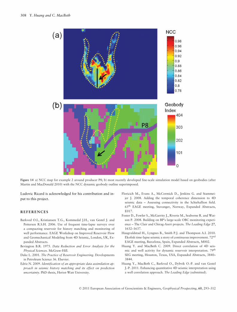
to the upper triangular compartment next to the heel of thewell. The shape of the seismic-derived anomaly suggests thatthe northern compartmental barrier may not be present andthat the north-south barriers between W2 and P8 need to bere-located. Interestingly, the most recent fine-scale simulationmodel for this field (Martin and MacDonald 2010) based ongeomodelling, shows an arcuate body around the toe of P8of similar dimensions and shape to the connected region im-aged by the NCC attribute (Fig. 14). There is also evidenceof a vertical barrier in our work in agreement with the geo-body interpretation and of a separate connected region to theeast of this feature into which W4 injects. It appears that

our proposed technique reveals a dynamically active geobodyconnected to the well.

D I S C U S S I O N

The technique introduced in this paper, outputs as a final com-posite product a thresholded seismic-derived map of cross-correlation values associated with the activity of a particularwell or well groups. These maps reveal a signal that appears toshow more well-centric, spatially contiguous and dynamicallyconnected regions than those seen by inspection of the 4Dseismic signatures individually. This can be explained by the



Figure 10 Right – correlation panels (right) for two specific locations (marked as 1 and 2 filled circles on the maps) around injector W3,comparing cumulative fluid volume changes (black dashed lines) and the corresponding 4D signatures (red dashed lines). Left – maps ofthe normalized cross-correlation attribute thresholded at a 99% confidence level. a) Results for observed 4D signatures; b) results for thecorresponding pressure change from the simulator, with an outline of saturation changes >20% drawn. Coloured lines are transmissibilitybarriers extracted from the simulator – barriers in both the x- and y-directions are combined.

action of the cross-correlation procedure, which is to ‘stack’and enhance all mapped seismic attributes that linearly cor-relate with the well/well group. Of course, as these cross-correlation values are thresholded, it should also be notedthat noise is still present in these results but it manifests it-self differently from the original input seismic. This particularnoise gives rise to small zones of high cross-correlation ly-ing outside the main signal, which are in fact non-productionrelated. As a simple comparison for the purposes of under-standing the 4D noise, the 4D signatures from the multiplesurveys are stacked (Fig. 15). This shows that amplitudes un-related to the well activity are included as noise in this pro-cess. It appears that our proposed technique preferentiallyselects the part of the 4D signature related only to pressureand derives the benefit of enhancing the seismic signal aroundonly the wells by combining a large number of frequently

repeated seismic in a specialized, engineering consistentmanner.

In order for the proposed technique to succeed, several con-ditions must be met. Firstly, the field must be surveyed by mul-tiple surveys and in particular enough surveys for the well toseismic cross-correlations to be significant to quantify. We an-ticipate there are now many such candidates that exist (Sandø,Munkvold and Elde 2009) and there is the expectation of fu-ture data sets (Watts 2011). If connected compartments (orgeobodies) around individual wells are to be ‘imaged’, thesewells must also possess distinctly different well rates, such thatthe correlation coefficient between the well and the 4D signa-tures is higher than the well to well correlation. The approachthus benefits from a sufficiently complicated well activity foreach time series of activity (switching wells on and off pro-vides a useful signal in our approach). In this respect it bears



Figure 11 Two 4D seismic signatures selected from the sequence of available data, with transmissibility barriers from the simulator superimposedfor reference. a) Signature for 04–96; b) signature for 02–96.

some similarities to well testing. Indeed, the proposed tech-nique resembles an extended well test, in that the response tovolume rate changes (not in this case build up or draw downhowever) induced at the well are detected and interpreted asdynamic boundaries. However, the scale for the extended welltest is several months, whereas for the seismic it ranges fromseveral months (the Valhall field) to a few years (the currentSchiehallion example). In contrast, pressure sensors in the wellare now replaced by mapped seismic attributes. In both, thesteady state condition is applied in a decline curve analysis,with the same objectives – to delineate barriers, volumes ofcompartments or geobodies in the reservoir. Once such re-gions have been identified, it is now possible to use these toupdate the simulation model and hence production forecasts.

Another important condition is that the chosen seismic at-tributes must be sensitive to reservoir pressure. The ideal sit-uation for the application of the method is pressure-sensitive4D signatures. For fields in which gas exsolves from a solutionor water saturation changes are a controlling influence overthe seismic, then the technique requires some adaptation. Thishas been considered in the work of Huang et al. (2011), whohave shown that in these situations the technique can still beused successfully. This also lends support to efforts which at-tempt to separate the effects of both pressure and saturationin 4D seismic (for example, Landrø 2001; Tura and Lumley2004; MacBeth et al. 2006). Finally, as most production andinjection volumes used in this procedure to date have beenmeasured as a comingled flow, the volume rates refer to the



Figure 12 a) Water saturation change predicted from the simulator for the 04–96 period; b) corresponding pressure change and c) gas saturationchange. White regions are inactive cells in the model.

whole completed interval rather than the particular reservoirover which the seismic attribute is defined. This is the correctapproach if the overall reservoir interval is thinner than theseismic wavelength but will not be appropriate for thick reser-

voir sequences. This could be improved if smart well technol-ogy is in place to observe the flow rates in specific flow units.However such technology is not commonly available in manymature fields.



Figure 13 Correlation panels (right) for two specific locations around the producer P8 (marked as 1 and 2 filled circles on the maps), comparingcumulative fluid volume changes (black dashed lines) and the corresponding 4D signatures (red dashed lines). Left – maps of the normalizedcross-correlation attribute thresholded at a 99% confidence level. a) Results for observed 4D signatures; b) map for the corresponding pressurechange from the simulator. Coloured lines are transmissibility barriers extracted from the simulator – barriers in both the x- and y-directionsare overlapped.

CONCLUSIONS

The concept of linking well activity (as defined by well vol-umes and rates) to 4D seismic signatures has been developedhere from a fundamental theory into a practical methodologyand applied to both model-based and field data. Using thisapproach a linear proportionality between mapped 4D seis-mic signatures from multiply acquired repeat surveys and thecumulative volumes produced or injected at wells over com-mon time periods is found. Performing a cross-correlationlinks the well data to the seismic data without using a simu-lation model. Application to a synthetic example shows thatthis cross-correlation method has the potential to delineatediscrete compartments or geobodies that are dynamically con-nected to a well or group of wells. Application to observationsfrom the Schiehallion field reveals well-centric connected geo-bodies and concludes that the geometry of these geobodiesdiffers from the static reservoir model built using the individ-ual seismic responses and geological information alone. This

suggests that the technique has future potential to be used asa tool to update the dynamic aspects of the simulation model,particularly transmissibility barriers. Other applications pub-lished by the authors (Huang et al. 2011; Huang and MacBeth2011) indicate that this approach can be applied successfullyto a variety of fields that have been frequently monitored.

ACKNOWLEDGEMENTS

We would like to thank the Schiehallion field partners (BP,Shell, Hess, Statoil, Murphy Petroleum and OMV) for pro-viding the data and permission to publish. We would alsolike to thank the sponsors of the Edinburgh Time LapseProject, Phase III and IV (BG, BP, Chevron, ConocoPhillips,EnCana, Eni, ExxonMobil, Hess, Ikon Science, Landmark,Maersk, Marathon, Norsar, Ohm, Petrobras, Shell, Statoil,Total and Woodside) for supporting this research. We thankSchlumberger-Geoquest for the use of their Petrel software.



Figure 14 a) NCC map for example 2 around producer P8; b) most recently developed fine-scale simulation model based on geobodies (afterMartin and MacDonald 2010) with the NCC dynamic geobody outline superimposed.

Ludovic Ricard is acknowledged for his contribution and in-put to this project.

REFERENCES

Barkved O.I., Kristiansen T.G., Kommedal J.H., van Gestel J. andPettersen R.S.H. 2006. Use of frequent time-lapse surveys overa compacting reservoir for history matching and monitoring ofwell performance. EAGE Workshop on Improved Reservoir Flowand Geomechanical Modeling from 4D Seismic, London, UK, Ex-panded Abstracts.

Bevington B.R. 1975. Data Reduction and Error Analysis for thePhysical Sciences. McGraw-Hill.

Dake L. 2001. The Practice of Reservoir Engineering. Developmentsin Petroleum Science 36. Elsevier.

Edriz N. 2009. Identification of an appropriate data assimilation ap-proach in seismic history matching and its effect on predictionuncertainty. PhD thesis, Heriot-Watt University.

Floricich M., Evans A., McCormick D., Jenkins G. and Stammei-jer J. 2008. Adding the temporal coherence dimension to 4Dseismic data – Assessing connectivity in the Schiehallion field.65th EAGE meeting, Stavanger, Norway, Expanded Abstracts,E017.

Foster D., Fowler S., McGarrity J., Riverie M., Seaborne R. and Wat-son P. 2008. Building on BP’s large-scale OBC monitoring experi-ence – The Clair and Chirag-Azeri projects. The Leading Edge 27,1632–1637.

Haugvaldstad H., Lyngnes B., Smith P.J. and Thompson A.I. 2010.Ekofisk time-lapse seismic a story of continuous improvement. 72nd

EAGE meeting, Barcelona, Spain, Expanded Abstracts, M002.Huang Y. and MacBeth C. 2009. Direct correlation of 4D seis-

mic and well activity for dynamic reservoir interpretation. 79th

SEG meeting, Houston, Texas, USA, Expanded Abstracts, 3840–3844.

Huang Y., MacBeth C., Barkved O., Dybvik O.-P. and van GestelJ.-P. 2011. Enhancing quantitative 4D seismic interpretation usinga well correlation approach. The Leading Edge (submitted).



Figure 15 Stacked difference maps for alltime intervals with all negative values beingconverted to positives.

Huang Y., MacBeth C., Barkved O. and van Gestel J.-P. 2011. En-hancing dynamic interpretation at the Valhall field by correlatingwell activity to 4D seismic signatures. First Break 29(3), 37–44.

Huang X., Will R. and Waggoner J. 2000. Reconciliation of time-lapse seismic data with production data for reservoir management:A Gulf of Mexico reservoir. 2000 SPE European Petroleum Con-ference, 24–25 October, Paris, France, Expanded Abstracts, SPE65155.

Landrø M. 2001. Discrimination between pressure and fluid sat-uration changes from time-lapse seismic data. Geophysics 66,836–844.

Leach H.M., Herbert N., Los A. and Smith R.L. 1999. The Schiehal-lion development. In: Petroleum Geology of Northwest Europe:Proceedings of the 5th Conference (eds A.J. Fleet and S.A.R. Boldy),pp. 683–692. Geological Society London.

MacBeth C., Floricich M. and Soldo J. 2006. Going quantitative with4D seismic analysis. Geophysical Prospecting 54, 303–317.

Martin K. and MacDonald C. 2010. The Schiehallion field: Applyinga geobody modelling approach to piece together a complex turbiditereservoir. DEVEX 2010, Expanded Abstracts, O.33

Morton A., Andersen M. and Thompson M. 2009. Field trial offocused seismic monitoring on the Snorre Field. 71st EAGE meeting,Amsterdam, the Netherlands, Expanded Abstracts, X026.

Osdal B. and Alsos T. 2010. Norne 4D and Reservoir Management– The keys to success. 65th EAGE meeting, Stavanger, Norway,Expanded Abstracts, L012.

Richardson S.M., Herbert N. and Leach H.M. 1997. How wellconnected is the Schiehallion reservoir? Proceedings of the Off-shore Europe Conference, Aberdeen, UK, Expanded Abstracts, SPE38560.



Sandø I., Munkvold O.P. and Elde R.M. 2009. Two decades of 4Dgeophysical developments – Experiences, value creation and futuretrends. World Oil 230(10).

Stephen K. and MacBeth C. 2006. Seismic history matching in theUKCS Schiehallion field. First Break 24, 43–49.

Stewart G. and Whaballa A.E. 1988. Pressure behaviour of compart-mentalised reservoir. 64th SPE Annual Technical Conference andExhibition, 8–11 October, San Antonio, Texas, USA, ExpandedAbstracts, SPE 19779

Tura A. and Lumley D.E. 1999. Estimating pressure and saturationchanges from time-lapse AVO data. 69th SEG meeting, Houston,Texas, USA, Expanded Abstracts, 1655–1658.

Watts G. 2011. EAGE Workshop on Permanent Reservoir Moni-toring Using Seismic Data. 28 February – 3 March, Trondheim,Norway, Expanded Abstracts.

AP PENDIX: L INK I N G C UMUL A T I V EV O L U M E T O P R E S S U R E C H A N G E : B A S I CCONCEPTS

The objective of this appendix is to define a relationship be-tween the pressure change, �P (as detected by the time-lapseseismic) and the change in the cumulative fluid volume �V

produced and injected over time intervals similar to thoseof most time-lapse seismic surveys (typically years). For thepurpose of this work, pressure changes are induced in thereservoir by the production of a volume of oil or water, orthe injection of water or gas. It is shown below that the re-lationship between the well activity and the pressure changesis governed by equations normally used in the context of welltesting. However, it should be noted that well testing con-cerns itself mainly with pressures measured in the boreholeover periods of hours or days at most, whilst our applicationconsiders pressure changes in the inter-well space over tensof months or several years. This difference in time scales andmeasurement location affects the choice of pressure solutionfor our particular objective.

When the well is put on flow at time t = 0 the oil productionrate is initially sustained by the expansion of fluid immedi-ately around the well-bore. This expansion is accompanied bya reduction in pressure and a pressure gradient is established.Fluid from the next outwardly adjacent annular zone flowstowards the wellbore and the process of fluid expansion andpressure decline is extended further into the reservoir. A pro-gressively increasing zone of pressure drawdown develops outfrom the active well. The evolution of the pressure around andaway from each well is governed by the pressure diffusivityequation, the particular well production/injectivity, well con-figurations and the boundary conditions associated with thereservoir. Consider a well that has started to produce from an

Figure A1 The regimes are defined by the different boundary con-ditions and different solutions to the problem of pressure evolutionin the reservoir. Exact time periods are important when consideringwell testing versus 4D seismic monitoring. The full line and dashedline refer to the different types of stable state flow.

initially untouched reservoir at virgin pressure. In terms of thephysical phenomena involved, several distinct time intervalsmust be distinguished (Fig. A1). At first a period of transientbehaviour persists, the exact duration of this depending uponthe diffusivity constant and hence the properties of the reser-voir around the well but being independent of the conditionsand geometry of the external reservoir boundaries. Duringproduction, any disturbance in the wells such as changingthe volume rate, or opening or closing a well to flow, willcreate a corresponding transient. This is analogous to the ac-tivation of an electrical switch and the subsequent electricalcurrent settling into a stable state. In this early stage regimethe pressure-transient solution to the diffusivity equation (seesection A.1 below) is relevant. This is also the region used forinterpreting the wellbore pressure changes in most well testliterature (see for example, Dake 2001). Following this inter-val is a complicated region of late transience, which is seldom



analysed in the literature due to the difficulties involved withobtaining an interpretable solution. Finally, when the pressuredisturbance has propagated at last to the outer boundaries ofthe reservoir or reservoir compartment, the evolution of pres-sure settles down into a stable equilibrium state. In this stablestate, the behaviour conforms to a well defined predictableform dependent on the boundary conditions and the pressurechange is now linear with time. It is this latter condition thatis appropriate for the 4D seismic analysis in our study (seeSection A.2).

A.1 Pressure transient behaviour and well testing change

Consider a single producing well flowing at a constant rateq into a homogeneous and isotropic porous reservoir of uni-form thickness h but infinite lateral extent. The reservoir isconsidered sufficiently large that the external boundary con-ditions are distant so that open flow boundary conditions canbe applied laterally, although it is closed and sealed by the topand base of the reservoir. Until the start of the production thereservoir is initially at a constant pressure Pinitial. Upon pro-duction, flow to the well is mostly radial and pressure dropsrapidly quite close to the wellbore and more slowly away fromthe well. In this condition, the local oil flow varies from a max-imum at the borehole to zero at the external boundary. Theevolution of the pressure at an arbitrary observation point aradial distance r from the well and at time t is governed pre-dominantly by the single phase, linearized diffusivity equationin a cylindrical coordinate system

μφct

k∂ P∂t

= ∂2 P∂ P2

+ 1r

∂ P∂r

, (A1)

where μ the viscosity, k the permeability, φ the porosity andct the total rock and fluid compressibility. In this equation allthe rock and fluid properties are assumed to be pressure in-dependent and the fluids only slightly compressible. Treatingthe well as a line source and initial conditions, the solution tothis equation is non-linear and given by (for example, Dake2001)

P(r, t) = Pinitial − qBoμ

2πkhEi

(φμctr2

4kt

), (A2)

where Ei is an exponential integral defined by Ei(x) =∫ ∞x

e−s

s ds and Bo is the oil volume formation factor, anapproximation of equation (A2) arises for the case whenx = φμctr2/4kt < 0.01

P(r, t) ≈ Pinitial − qBo

2πkhln

(1.781φμctr2

4kt

). (A3)

This form of the equation is commonly used as the basis forwell testing interpretation. In the case of well testing, despitethe times being only a few hours, x is typically less than 0.01as all measurements are made at the well, so that r is thewellbore radius. Well to well interference tests, where thepressure is measured in an inactive observation well at somedistance r from the flowing well, are taken over by largertimes and thus the approximate solution can thus be used forinterpretation. If barriers or discontinuities defined by faults,stratigraphic pinchouts or shale barriers are encountered, thensmall perturbations in the pressure decay profile of equation(A3) can be noted and used to infer their location and reservoirsignificance.

A.2 The stable state and global reservoir pressure

The stable state is mostly ignored by well testers but is ofvalue to those wishing to pursue decline curve analysis. Thevelocity with which the pressure disturbance moves throughthe reservoir is determined by the porosity, permeability, vis-cosity and total compressibility. The leading edge of this pres-sure disturbance, the pressure front, is usually defined looselyas the location where the pressure is 1% of the initial valuePinitial. The time to propagate a radial distance rb to the nearestboundary is (Stewart and Whaballa 1988)

t ≥ 497.6r2

b φμct

k, (A4)

where μ is in cP, ct in psi−1, rb in metres, k in mD and t indays. As an example related to the Schiehallion field from themain text, if φ = 28%, μ = 3.2cP, ct = 2.2.10−5psi−1, k =280 mD and rb = 900 m then equation (A4) gives approxi-mately 26 days. Note that the time at which the stable statesolution becomes important and a measure of the extent be-fore the system is disturbed by the outer boundary condition,is usually 1 to 1.5 times this number. Interestingly, the depar-ture from the transient period can be used in transient welltesting to determine the permeability of the reservoir if rb andthe reservoir properties are known. Importantly, the time pe-riod over which seismic surveys are repeated is always muchgreater than the duration of the transients. It thus appears thatfor most 4D surveys the steady state condition is immediatelyapplicable.

The steady state solution of the diffusivity equation is ob-served by recognizing the stability of the pressure distributionover time. In a balanced waterflood, for example, the totalrate of water injection (and aquifer influx if appropriate) isequal to the total rate of oil produced such that for the pres-



sure, P, at any location throughout the reservoir volume ofinterest the condition ∂ P/∂t = 0 is fulfilled. In many reservoirsituations there is no natural water influx and in the absenceof fluid injection, oil production results solely in the expansionof oil in place and the reservoir pressure is reduced. When thepressure disturbance propagates outwards and encounters theouter sealing boundary of the reservoir compartment, no flowis allowed and this leads to an overall pressure decline. Therate of pressure decline is obtained by equating the productionrate, q = ∂V/.∂t, at the well to the overall volume rate of fluidexpansion within the drainage region V and considering thetotal compressibility ct = − 1

V ( ∂V∂ P ). This leads to the relation

q = −ctV∂ P∂t

, (A5)

or

∂ P∂t

= − 1ctV

q. (A6)

Thus, if we produce a reservoir compartment at a constantrate q, after the period of transience the rate of pressure de-cline ∂ P/∂t for all radial distances from the well is constantand uniform. Note that the pressure profile in the reservoirstill remains relatively complex but the pressure drop is quitesimple and predictable. The condition for which there are reg-ular changes with time but pressure still declines as in equation(A6) is known as the semi steady state in well testing litera-ture. From equation (A6) we observe that the rate at which thepressure declines depends on the compartment volume and itstotal compressibility and the well rate.

A.3 Connection between pressure change and the wells

By rearranging equation (A6) and integrating over the timeperiod �T between a baseline and monitor seismic survey, thecorresponding pressure drop �P at all distances and locationsin the compartment from the well (and hence the 4D seismicresponse) can be written in terms of the difference of thecumulative volume produced �Vf (= q�T)

�P = − 1ctV

�Vf . (A7)

Thus, the pressure drop in the reservoir is proportional tothe cumulative volume of oil produced from the formation.This equation can be extended to include M wells injectinginto (constant positive rate qI) and N wells producing oil and

water from (constant negative rates qP and qPW respectively)the reservoir by applying the principle of superposition (Dake2001), which permits linear combinations of solutions

�P = 1ctV

⎛⎝Bw

M∑i=1

qIi + Bo

N∑j=1

qPj + Bw

N∑j=1

qPWj

⎞⎠ �T.

(A8)

The produced volumes at the surface must be adjusted by for-mation volume factors, Bw and Bo, to the formation volumes.Furthermore, superposition states that if each well experi-ences a different sequence of constant rates, the equation canbe generalized further

�P = 1ctV

⎛⎝Bw

M∑i=1

mi∑k=1

qIik�Tik + Bo

N∑j=1

n j∑l=1

qPil �Tjl

+Bw

N∑j=1

n j∑l=1

qPWil �Tjl

⎞⎠ , (A9)

where mi and nj are the segments of times for the ith injectorand jth producer over which the rates are held fixed. Thus, ifseveral repeated 4D surveys are shot, the pressure drop mea-sured at the time of each survey can be related directly to thecumulative well data only if the surveys are not shot duringa transient period (that is, the well start-up, closure, or ratechange). Interestingly, this predicts that for a constant ratethroughout the period �T and for all repeated surveys, thepressure drop is proportional to the duration of the time pe-riod and can be correlated directly to the duration between thesurveys. If the wells are producing at a constant rate duringthe time at which all surveys are being shot, then the pressuredrops (and hence seismic signature change) simply respondand are correlated to the length of the time period. If thewells change their rates frequently, then the pressure drops inthe compartment can be directly correlated to the cumulativevolumes produced and injected (the large bracketed term onthe right-hand side of equation (A8)). In practice this termmay become an integral over time due to the small-scale wellfluctuations. In the main text, this correlation is utilized tounderstand the pressure signal for a sequence of many timelapse seismic surveys. Importantly, this equation holds regard-less of the well positioning in the compartment, the shape ofthe compartment and the exact nature of the boundary con-ditions (the steady state solution naturally follows by setting�V = 0).


Date post:	27-Dec-2021
Category:	Documents
Upload:	others
View:	4 times
Download:	0 times

Direct correlation of 4D seismic with well activity for a ...

Documents