Direct Raman Imaging Techniques for Studying

the Subcellular Distribution of a Drug

*Jian Ling1

Steven D. Weitman2

Michael A. Miller1

Rodney V. Moore2

Alan C. Bovik3

1Southwest Research Institute, Bioengineering Department6220 Culebra Rd., San Antonio, Texas 78238, USA

2Institute for Drug Development14960 Omicron Dr., San Antonio, Texas 78245, USA

3The University of Texas at AustinDepartment of Electrical and Computer Engineering

Austin, Texas 78712, USA

* Correspondence to:Jian Ling, Ph.D.Bioengineering DepartmentSouthwest Research Institute6220 Culebra RoadSan Antonio, TX 78238Tel: (210) 522-3953Fax: (210) 684-6147Email: jling@swri.org

ABSTRACT

Direct Raman imaging techniques are demonstrated to study the drug distribution

in living cells. The advantage of Raman imaging is that no external markers are required,

which simplify the sample preparation and minimally disturbs the drug mechanism

during imaging. The major challenge in Raman imaging is the very weak Raman signal.

In this study, we presented a Raman image model to describe the degradation of Raman

signals by imaging processes. Using this model, special-purpose image-processing

algorithms were demonstrated to restore the Raman images. The processing techniques

were then applied to visualize the anticancer agent paclitaxel in living MDA-435 breast

cancer cells. Raman images were obtained from a cancer cell before, during, and after the

drug treatment. The paclitaxel distribution illustrated in these images is explained by the

binding characteristics of the paclitaxel and its molecular target – the microtubules. This

result demonstrates that direct Raman imaging is a promising tool to study the

distribution of a drug in living cells.

1

INTRODUCTION

The recent implementation of rational drug design, combinatorial chemistry

techniques, and high throughput screening have led to large numbers of new drug leads.

There is a tremendous need for cost-effective and efficient approaches to evaluate the

efficacy of these potential drugs. Early assessment of drug efficacy is critical for

pharmaceutical companies because it will save millions of dollars that would otherwise

be spent on animal and clinical studies on less efficient drug leads.

A cost-effective way of evaluating drug efficacy at the early stage of drug

development is to understand its action at the cellular level 1, 2. For example, the cellular

uptake, intracellular distribution, binding characteristics, intracellular pharmacokinetics,

and cellular resistance of a drug generally determine the efficacy of the drug.

Laser scanning fluorescence microscopy has been used for the in vitro study of

drug action at the cellular level for many years 3-10. However, the auto-fluorescence of

most drugs is weak and unspecific (broad bandwidth), therefore, molecular-specific

images often cannot be acquired by imaging of auto-fluorescence. Instead, certain

fluorophores need to be used as a fluorescing label to selectively bind to specific regions

of the drug molecules by chemical or physical means before imaging 11, 12. The need to

prepare and, subsequently, test external markers or labels often complicates the

assessment of drug action. In addition, using a relatively large fluorophore molecule as a

tag on to a (often smaller) drug molecule can potentially change the activities of the drug

in tumor cells. The fluorescent markers used in the specimen may cause undesirable

pharmacological or toxicological effects. Also, a suitable marker is often not available

2

for all bio-molecules. The continuous loss of fluorescence intensity during measurement

due to photon bleaching, and the potential for photo-damage to the bio-specimen due to

the use of ultraviolet wavelengths, are also fundamental problems of fluorescence

microscopy.

The Raman spectrum of a particular substance depends on the structure

(vibrational states of chemical bonds) of the molecules, and therefore it can identify a

particular type of molecule by its unique combination of scattered frequencies (also

referred to as Raman peaks or Raman modes). Raman imaging can provide an overview

of the spatial arrangement of a particular type of molecule within a heterogeneous

specimen. Raman imaging requires no external markers, dyes, or labels as required in

fluorescent imaging. In addition, the near-infrared excitation used in Raman imaging of

the present work has a number of advantages for biological systems, such as producing

less laser-induced fluorescence and photo-thermal degradation, and allowing better

perspective depth (>1 mm) into a sample 13, 14.

The major challenge in Raman applications is the inherently weak signals in

Raman scattering comparing to the signals in Rayleigh scattering or fluorescence. Raman

imaging, especially direct Raman imaging, was not practical until the recent development

of robust laser sources and low-noise CCD (charge-coupled device) detectors 15, 16. For

many years Raman images have been acquired by pixel-to-pixel (or line-to-line) laser-

scanning methods 17-22. Because the Raman signal is weak and takes a relatively long

time to obtain the spectrum for each pixel, the scanning time for a whole image is

considerable. For example, complete scanning of a 128x128-pixel Raman image using

3

point illumination may take overnight, which is not a suitable scanning rate for living cell

studies.

With the inventions of dielectric filters 23, acousto-optic tunable filters (AOTF) 24,

and liquid crystal tunable filters (LCTF) 25-27, direct (or wide field) Raman imaging

became an alternative imaging method. Direct Raman images are acquired at a selected

Raman mode from a sample that is globally illuminated by an expanded laser beam

(Figure 1). The imaging time is equivalent to the scanning time for one pixel in the laser-

scanning method. In addition, the fidelity of the direct Raman images is primarily limited

by the objective lens used in the microscope. Therefore, direct Raman imaging has the

potential to provide an efficient way of obtaining high-definition Raman images. Direct

Raman imaging has been used to study the distribution of the non-fluorescent

photodynamic therapy agent cobalt-octacarboxy phthalocyanine [CoOCP] inside the

K562 leukemia cells 28-30. These studies suggest the potential application of Raman

imaging in drug research. However, in order to extract correct and useful information

from Raman images with weak signals, a systematic procedure is required.

In this paper, a model was first developed for direct Raman microscopic images to

describe the degradation of Raman signals by several processes: non-uniform

illumination of the laser excitation source, distortion by the microscope system, and the

influence of additive signal-dependent Gaussian noise. Using this model, image-

processing algorithms were demonstrated to restore a recorded Raman image into a

considerably improved image that better reflects the molecular distributions.

The general Raman imaging and data analysis techniques were then applied to the

visualization of an anticancer drug – paclitaxel within living tumor cells. Paclitaxel is an

important antimitotic agent for which the mechanisms of interaction with a cell are well-

established 31-34 and is a suitable candidate for validation of Raman imaging capabilities.

MODELING AND PROCESSING OF DIRECT RAMAN IMAGES

Assume a laser beam illuminates at a focal plane (z) inside a three-dimensional

specimen. The Raman scattering coefficient for the heterogeneous area is K(x,y,z), which

is proportional to the concentration of specific chemical bonds to be imaged. The

fluorescence signal from the heterogeneous specimen is K0(x,y,z). Then the scattering

signal s(x,y,z) can be modeled as:

( ) ( ) ( )[ ] ( ) tyxizyxKzyxKzyxs ××+= ,,,,,,, 0 ,

where t is the exposure time. Usually the intensity of the illumination at the focal pla

not uniform but dependent on the locations (x,y) due to the imperfections in the

expanding system. This lack of homogeneity of the illumination, indicated by i(

causes a non-uniform illumination effect in the recorded images.

A direct Raman image is a wide-field image that is taken at a specific focal p

within a sample. However, this image is the sum of in-focus information from the f

plane and out-of-focus information from the neighborhood planes due to the f

recording aperture and the limited depth of focus of the imaging system 35, 36. In o

words, the Raman signal s(x,y,z) is blurred by the microscopic system. This blu

characterized in terms of the microscope’s point spread function (PSF) h(x,y,z) o

(1)

4

ne is

laser

x,y),

lane

ocal

inite

ther

r is

r its

Fourier transform, the optical transfer function (OTF). If the image formation system is

assumed to be linear and time-invariant, then the recorded image g(x,y,z) can be

represented as:

( ) ( ){ ( ) ( )[ ]} ( ) ( )zyxntyxizyxKzyxKzyxhzyxg ,,,,,,,,,,, 0 +××+∗= ,

where * is the linear convolution operator. The blurred Raman signal was further

degraded by the additive noise n(x,y,z) that occurs during image recording.

The purpose of the Raman image processing is to determine the Raman scattering

coefficient K(x,y,z) of the imaging area from the recorded image g(x,y,z). In order to

determine K(x,y,z), it is necessary to reduce the noise n(x,y,z) from the image g(x,y,z), to

correct the non-uniform illumination i(x,y), to deconvolve with the point-spread function

h(x,y,z), and to subtract the fluorescence signal K0(x,y,z).

Noise Reduction Using Anisotropic Median-Diffusion Filter

A Raman image is a molecular image, which displays the distribution of

molecules. Such an image can be modeled as a piecewise-smooth image, which can be

divided into several regions. Each region is chosen such that the changes in molecular

concentration within the region are small and gradual. The intensities between the

different regions are quite dissimilar because of the significant difference in molecular

concentration. For these kind of piecewise-smooth images, the anisotropic median-

diffusion filter was found 37 to be a suitable denoising filter. The anisotropic median-

diffusion filter is described as:

[ ] )()()1(

4n

WWEESSNNnn gcgcgcgcgg ∇+∇+∇+∇+=+ λ ,

),( )1()1( WindowgerMedianFiltg nn ++ = ,

(3)

(2)

5

where (n) and (n+1) are the number of iterations, and λ ∈ [0,1] controls the rate of the

diffusion. The idea behind the anisotropic median-diffusion filter is to evolve from the

recorded noisy image g(0) a family of increasingly smooth images g(n) to estimate the

original image.

The letters N,S,E,W in Eq. 3 are mnemonics for North, South, East and West; they

describe the direction of the local gradient. The local gradient of an image at any iteration

is calculated by the difference in the nearest-neighbor pixels:

jijijiW

jijijiE

jijijiS

jijijiN

gggggggggggg

,1,,

,1,,

,,1,

,,1,

−=∇

−=∇

−=∇

−=∇

−

+

+

−

.

The diffusion coefficients cN , cS , cE , cW are the function of the local gradients ∇ N g, ∇ S g,

∇ E g, and ∇ W g, respectively. The Tukey biweight norm proposed by Black et al. 38 is

used as the diffusion function. The normalized (magnitude) Tukey biweight diffusion

coefficient is defined as:

( ) ( )

≤∇

∇−=∇

otherwise

KgKgKKgc

0

5511625

,22

,

where K is the threshold of the local gradients, which is tuned for a particular applic

The Window in Eq. 3 is the window for the median operator. A 3x3 window is u

used.

The anisotropic median-diffusion filter is especially useful to smooth image

low signal-to-noise ratio, such as the Raman images. It can effectively reduc

Gaussian noise without blurring the edges on the images. A quantitative study has s

(5)

(4)

6

ation.

sually

s with

e the

hown

that the anisotropic median-diffusion smoothed images are very close to the original

images in correlation, mean luminance and contrast 37.

Correction of Non-uniform Illumination

After reducing the noise, the non-uniform illumination i(x,y) needs to be corrected

(see Equation 2). A flat field image is used as a reference image to correct the lateral non-

uniform illumination. The effect of illumination difference in the axial direction is

considered in PSF.

According to the image model, a recorded flat-field reference image (after

smoothing) can be expressed as:

( ) ( ) ( ) tyxiKyxhyxr flat ××= ,]*,[, ,

where Kflat is a constant here. The residue noise after smoothing is ignored in Eq. 6 for

simplicity. The OTF of a microscope system is usually a low-pass filter (for example, the

microscope system used in this research has a lateral cut-off frequency of 0.57 µm-1 and

an axial cut-off frequency of 0.15 µm-1). Therefore, Eq. 6 can be simplified to:

( ) ( ) tyxiKyxr flat ××= ,, ,

because of the “zero” frequency characteristics of the Kflat. The reference image is

normalized by its own median value to give the compensating image c(x,y):

( ))],([

),()],([

),(,yxiMedian

yxiyxrMedian

yxryxc == .

Dividing c(x,y) by the denoised Raman image gs(x,y,z) we get the compensated imag

( ) [ ] tyxiMedianzyxKzyxKzyxhyxc

zyxgzyxg sc ××+∗== )],([}),,(),,(),,({

),(),,(,, 0 .

)

(7)

then

(8)

e:

)

(9

(6

7

8

The above compensation algorithm keeps the median intensity of the image

unchanged. This algorithm is based on the assumptions that the Raman scattering

coefficient is linearly related to the exposure time. It is also important to smooth the

image before the compensation. Otherwise, the noise may be amplified after the

compensation algorithm.

Three-dimensional Image Deconvolution

The objective of three-dimensional deconvolution is to restore the blurred image

by using the PSF of the imaging system. After the deconvolution, it will reduce the in-

focus-plane blurs caused by the limited aperture of the system as well as the out-of-focus-

plane blurs resulted from the limited depth-of-field of the system.

Many three-dimensional deconvolution algorithms have been developed,

including the inverse filter, the Wiener filter, the Nearest-Neighbor deconvolution, the

constrained iterative method, and the expectation-maximization maximum-likelihood

(EM-ML) deconvolution. When restoring an image with all the information at the

neighborhood planes available and no noise present, the deconvolution results from all

these algorithms are very similar. However, in practice, some amount of noise always

exists in a recorded image, even after smoothing by the anisotropic median-diffusion

filter. In addition, there are often only a few images that can be recorded at different

defocus planes within a limited period of time. Especially in the case of Raman imaging

of living cells, we were only able to get one image (at a specific focal plane) to represent

the drug distributions using the current instrumentation. This is again due to the relatively

long exposure time required for Raman imaging.

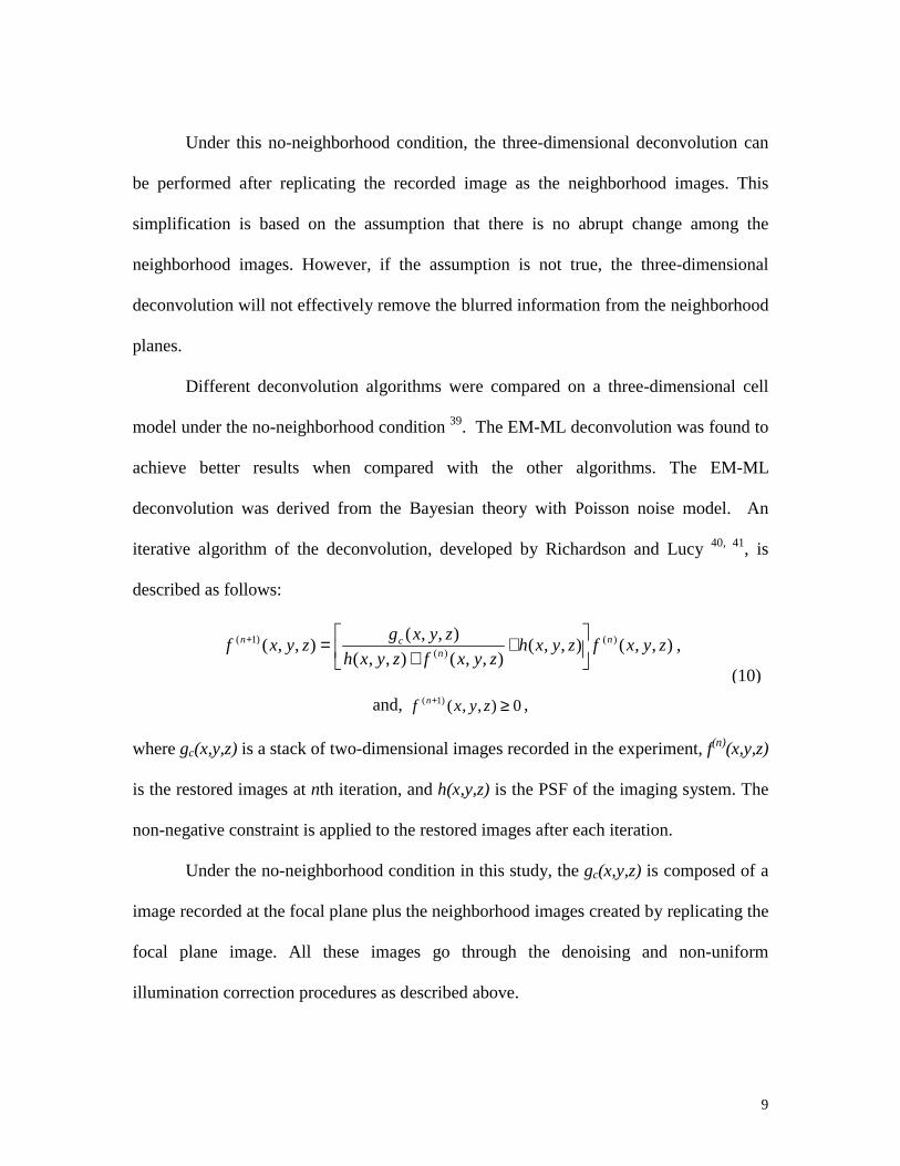
Under this no-neighborhood condition, the three-dimensional deconvolution can

be performed after replicating the recorded image as the neighborhood images. This

simplification is based on the assumption that there is no abrupt change among the

neighborhood images. However, if the assumption is not true, the three-dimensional

deconvolution will not effectively remove the blurred information from the neighborhood

planes.

Different deconvolution algorithms were compared on a three-dimensional cell

model under the no-neighborhood condition 39. The EM-ML deconvolution was found to

achieve better results when compared with the other algorithms. The EM-ML

deconvolution was derived from the Bayesian theory with Poisson noise model. An

iterative algorithm of the deconvolution, developed by Richardson and Lucy 40, 41, is

described as follows:

),,(),,(),,(),,(

),,(),,( )()(

)1( zyxfzyxhzyxfzyxh

zyxgzyxf nn

cn

∗∗

=+ ,

and, 0),,()1( ≥+ zyxf n ,

where gc(x,y,z) is a stack of two-dimensional images recorded in the experiment, f(n

is the restored images at nth iteration, and h(x,y,z) is the PSF of the imaging system

non-negative constraint is applied to the restored images after each iteration.

Under the no-neighborhood condition in this study, the gc(x,y,z) is compose

image recorded at the focal plane plus the neighborhood images created by replicati

focal plane image. All these images go through the denoising and non-un

illumination correction procedures as described above.

(10)

9

)(x,y,z)

. The

d of a

ng the

iform

It is also important to subtract the background, or the “DC” value from the images

prior to performing the deconvolution. Studies 42, 43 have shown that the background

intensity has critical influence on the performance of the EM-ML deconvolution. This is

because the existence of the background makes the nonnegative constraint less effective.

In this study, the image background could be the fluorescence from the aqueous solution,

which can be assumed uniform across the image. This background was subtracted from

gc(x,y,z) before deconvolution.

Elimination of Fluorescence Signal

After deconvolution, Equation 2 became:

( ) ( ) ( )zyxKzyxKzyxf ,,,,,, 0+= .

The next processing step is to subtract the fluorescent signal K0(x,y,z). The fluores

signal is different from the fluorescence background discussed above. It is genera

the specimen, so it is usually non-uniform due to the heterogeneity of the specimen

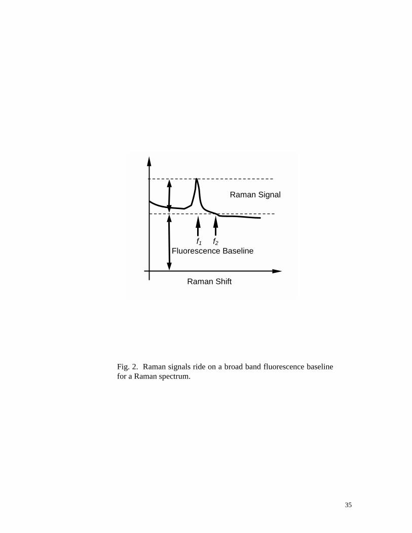
estimation of this fluorescent signal is done according to the properties of a R

spectrum. A Raman spectrum is composed of narrow-band Raman signals

broadband fluorescence baseline (Figure 2). The Raman signals ride on the broa

fluorescence baseline. If a Raman image is taken at the frequency of f1, its fluor

signal can be best estimated from another image taken at a neighborhood frequen

This is because an image at neighborhood frequency f2 shares the same fluores

distributions as at the f1 but without Raman signal. This neighborhood image c

through the same processing as discussed above to get the fluorescent signal K0(

which can then be directly subtracted from Equation 11.

)

(11

10

cence

ted by

. The

aman

and a

dband

escent

cy f2.

cence

an go

x,y,z),

11

EXPERIMENT AND DATA ANALYSIS

Instrumentation

A Renishaw Model 2000 Raman spectroscopic system (Gloucestershire, UK,

1993) was used in the study. This system is capable of acquiring Raman spectra, laser-

scanning Raman spectroscopic images, and direct Raman images with an expanded laser

beam. A Ti:Sapphire laser system (Lexel Laser Inc., California) was established for the

Raman system to replace the 30 mW diode laser originally equipped with the Raman

system. The diode laser source is suitable for Raman spectroscopy on biological samples.

However, when the laser is used for direct imaging, the beam must be expanded and

spread over thousands of pixels. In such applications, it provides inadequate illumination

power. In addition, the diode laser source has a line-shape beam so that the imaging area

suffers severe non-uniform illumination. The Ti:Sapphire laser, pumped by a 7W argon-

ion laser (Lexel 95-7), emits near-infrared wavelength with the maximum power of 1 W.

The Ti:Sapphire laser also has a Gaussian beam shape which greatly improves the beam

quality after beam expansion. In this study the laser was tuned to 782 nm to match the

holographic notch filter in the Raman system.

The Raman system can achieve spectral resolution of 1 cm-1 for spectrum

measurement with a grating system. For direct imaging, the dielectric filter has a

bandwidth of 10-20 cm-1. The Raman system is placed in a dark room and is stabilized on

an anti-vibration table (Vibraplane Air Suspension System, Kinetic System, Inc., Boston,

USA). This setup provides an ideal imaging environment.

12

A 60X Olympus water-immersion, high infrared transmission (71%) objective lens

(1-UM571 LUMPLFL 60x W/IR, Olympus, Japan) was used to obtain images of living

cells incubated in aqueous solution. This lens has a numerical aperture (NA) of 0.90 and

a depth of field (DOF) of 1.2 µm. The diffraction-limited optical resolution of this lens

can be calculated by Abbe’s equation:

.61.0NA

s λ=

In this study, the excitation wavelength is λ = 782, the maximum resolution that can be

achieved is about 0.53 µm. The resolution of the system is also affected by the

magnification of the microscope, the pixel size of the CCD camera, and the sampling

rate. The complete optical characteristics of the Raman system is determined by its PSF

(or OTF), which was estimated in this study by using small polystyrene microspheres

(0.2 µm in diameter) as the point light source39. This PSF will be used in three-

dimensional deconvolution.

The Raman Band for Imaging the Drug

Paclitaxel is an anticancer drug often used to treat breast cancer, ovarian cancer,

and non-small cell lung cancer. Paclitaxel was selected for this study because its

interactions with cellular molecules have been well studied. This knowledge will help us

examine the results and determine the capability of the Raman imaging technology.

Figure 3 illustrates the chemical structure of paclitaxel and its Raman spectrum of

pure powder (Yunnan Hande Technology Development Co. Ltd., Kunming, China). The

most significant Raman peaks of paclitaxel are at 617 cm-1, 1002 cm-1, and 1601 cm-1.

(12)

13

The Raman peak at 617 cm-1 is due to deformation of benzene rings in the structure. The

Raman peak at 1002 cm-1 is due to the sp3 hybridized carbon-carbon (C-C) vibration. The

Raman peak at 1601 cm-1 is due to the carbon-carbon double bond (C=C) stretching

vibration.

The powder paclitaxel, however, is not soluble in water, thus it cannot be used to

treat cells directly. According to the clinical formula of the drug (Bristol-Myers Squibb

Company, Princeton, NJ), paclitaxel was first dissolved in dehydrate ethanol alcohol and

cremophor EL (polyoxyethylated castor oil) and then further diluted with phosphate

buffered saline (PBS) solution. With the mix of ethanol and cremophor oil, the Raman

spectrum of the paclitaxel solution was affected significantly. Figure 4 illustrates the

Raman spectrum (with no fluorescence baseline correction) of a 0.3mg/ml (350 µM)

paclitaxel solution between 750 and 1250 cm-1. The strong fluorescence baseline from

cremophor oil and ethanol swamped most of the Raman peaks of paclitaxel, but leaving

the peak at 1002 cm-1 (shift to 1000 cm-1). Fortunately, neither ethanol nor cremophor oil

has Raman peak around 1000 cm-1.

In order to detect paclitaxel in a cell, Raman and fluorescent signals from a cell

also need to be studied. In this study, the human breast tumor cell line, MDA-435, was

used. Figure 5 shows the Raman spectrum (with no fluorescence baseline correction) of

the cytoplasm (at one local spot) of an MDA-435 breast tumor cell. The Raman spectrum

of the cell nucleus (not shown here) is very similar to the spectrum of the cytoplasm. The

carbon-carbon stretching mode (at the Raman peak about 1003 cm-1) from the molecules

(proteins) inside cell is also presented on the cell spectrum. This peak is very close to the

14

1000 cm-1 Raman band that we will use for detecting the paclitaxel. Fortunately, the

Raman signal at this peak from the cell is relatively weaker than that from the paclitaxel,

thus the intrinsic Raman signal from the cell should have a small contribution to the

Raman image at 1000 cm-1. To further distinguish the changes of Raman signals before

and after drug treatment, the Raman images before the cell exposure to the paclitaxel

solution will be used as the control case to be compared with the Raman images after the

drug treatment. In summary, one Raman image will be taken at 1000 cm-1 to detect the

paclitaxel. Another Raman image will be taken at 1080 cm-1 to correct the contribution of

fluorescent signal on the 1000 cm-1 image.

Cell Preparation and Imaging Procedure

Approximately 105 MDA-435 breast tumor cells were cultured on a gold-coated

Petri dish and allowed to stabilize for 24 hours in RPMI-1640 medium supplemented

with fetal bovine serum. After stabilization, the cells adhered to the bottom of the Petri

dish.

Before imaging, the RPMI nutrition medium was washed out with PBS. PBS was

used as the medium during imaging to reduce the fluorescent background from the

nutrition medium. Three cell images were taken before paclitaxel treatment. A white light

image of the cell illustrates the cell structure. A corresponding Raman image of the same

cell was taken at the 1000 cm-1 Raman band. This image records both the Raman signal

and the fluorescent signal from the cell. A second Raman image was taken at 1080 cm-1,

which only has the contribution from fluorescent signals. These three images form an

image record under control situation.

15

After taking images in a control situation, PBS was then replaced by the 0.3

mg/ml (or 350 µM) paclitaxel solution to start the drug treatment. The cells were exposed

to paclitaxel for one hour. During the one-hour drug treatment, the same images were

recorded to show the cellular distributions of paclitaxel during the drug treatment. After

one hour of treatment, the paclitaxel solution was washed out using PBS, and the cells

were returned to the PBS medium. Images were then acquired to show the drug retained

by the cell.

Data Processing and Analysis

As described above, each image record contains a white light image and two

Raman images at 1000 cm-1 and 1080 cm-1, respectively. An example of such a record

plus the direct difference of two Raman images are shown in Figure 6. It is obviously

difficult to get useful information from the raw data before processing. The image

processing algorithms developed based on the Raman imaging model were then used to

explore the data step by step.

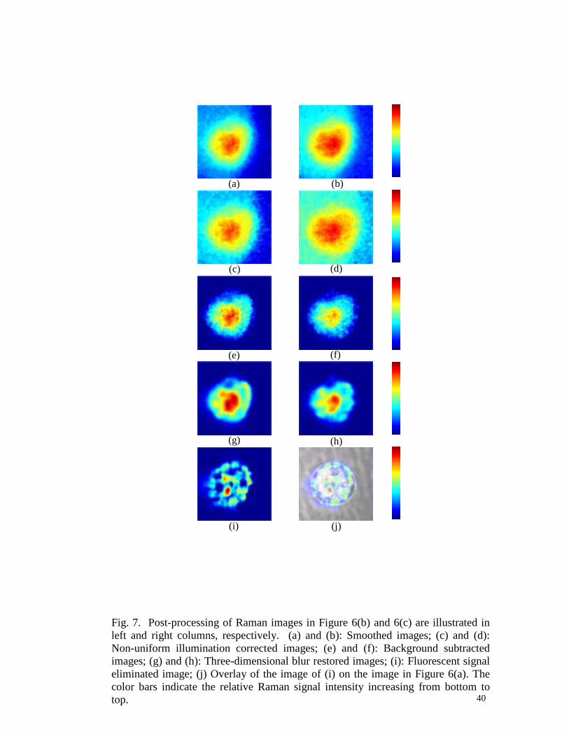
Figures 7(a) and (b) illustrate the Raman images after reducing the noise using the

anisotropic median-diffusion filter. The standard deviation of the image gradient was

used as the threshold in diffusion coefficient. A 3x3 window was used for the median

filter.

Figures 7(c) and (d) show the Raman images with the non-uniform illumination

corrected. A Raman image of a flat surface was recorded before each experiment as the

reference illumination.

16

Figures 7(e) and (f) show the images after subtracting their fluorescence

background. This background is the fluorescent intensity contributed from the PBS

solution. Therefore, it is uniform across the image, like a “DC” component. The

fluorescent signal contributed from the intracellular structure, however, is not uniform

due to the heterogeneity of the cell. That part of the fluorescence is referred to as the

“AC” component in this paper. That fluorescence signal is handled in Figure 7(h).

A simple way of eliminating the fluorescence “DC” background is to subtract the

average value of the image and then to set all the negative values to zero. This simplified

method is only suitable when the background occupies most of the area of an image. In

this case, the average value of the image is close to the “DC” background. The

subtraction of average value also enhanced the image; only intensity (fluorescence “AC”

component plus Raman signal) higher than the average value was left on the image. The

Raman image in Figure 7(e) contains the Raman signal at the 1000 cm-1 band as well as

the fluorescent “AC” component in this band. The image in Figure 7(f), however,

contains the same fluorescent “AC” component as in the 1000 cm-1 band but without the

Raman signal. Most importantly, the background subtraction makes the three-

dimensional restoration more effective as discussed in the deconvolution section above.

Figures 7(g) and 7(h) illustrate the restored images using the EM-ML three-

dimensional deconvolution algorithm. The OTF of the Raman system, determined

through measurement, was used here for the deconvolution.

Finally, the Raman image at 1080 cm-1 in Figure 7(h) was subtracted from the

Raman image at 1000 cm-1 in Figure 7(g). The image after eliminating the fluorescence

17

signal is shown in Figure 7(i), which illustrates the paclitaxel distributions. The

superimposition of the paclitaxel distribution image and the white light image in Figure

6(a) is shown in Figure 7(j), which illustrates the paclitaxel distribution in the cell.

RESULTS AND DISCUSSIONS

MD-435 tumor cells were exposed to the 0.3 mg/ml (or 350 µM) paclitaxel

solution for one hour. The white light images and Raman images were obtained before,

during, and after the Paclitaxel treatment (Figure 8). All the Raman images were taken

using a 60x water immersion lens with the exposure time of 300 seconds. They were

processed using the method described above.

The first row in Figure 8 illustrates the images before drug treatment. These

images show the 1000 cm-1 Raman signals contributed from the molecules of the cell

itself. From the overlay image, the intrinsic Raman signals appear outside of the cell. It

cannot be the line up problem because the white light image and Raman image are

registered with 1 µm microspheres before the experiment. Most probably, the problem is

due to the imaging focal plane not being at the largest cross-area of the cell. Please note

there is a halo outside the cell, that may be the real cell boundary. The strong Raman

signal in the corresponding Raman image could be the contribution from the

neighborhood planes. This neighborhood information may not be removed effectively by

the three-dimensional deconvolution due to the no-neighborhood condition (see the

section of three-dimensional image deconvolution). Nevertheless, this image does show

that the original Raman intensities inside this cell are relatively low.

18

The second and third rows in Figure 8 illustrate the images 10 minutes and 45

minutes into the drug treatment. These images suggest that the paclitaxel were

accumulated outside the cell membrane and were gradually diffusing into the cell. The

relative low Raman intensities in these two figures are probably because the cell is not in

the PBS solution but in the drug solution, which contributes to a higher background than

the PBS solution. After subtracting a higher average value from the image, its intensity

became lower. In other words, the Raman intensities shown in the figures are relative

after subtracting their average value. Therefore, the quantitative information was not

preserved.

The fourth row through the seventh row in Figure 8 illustrate the images 10

minutes, 1.75 hours, 4 hours, and 4.5 hours after the drug treatment (after the paclitaxel

agent was washed out). These images show that the Raman intensities are relatively

higher in the center area as well as near the cell membrane. However, there is no

intensity in the cell nucleus area. As we know, the Raman signal is directly related to the

molecular concentration. The higher the intensity, the higher the molecular

concentration. Therefore, these figures suggest that paclitaxel is more concentrated near

the center of the cell as well as near the cell membrane, but less concentrated in the cell

nucleus. The finding of paclitaxel distributions from the Raman images is explained by

the binding characteristics of the paclitaxel and its molecular target – the microtubules.

Paclitaxel is an antimitotic drug, which stabilizes the microtubules, one type of

cytoskeleton that plays an important role in cell division. Microtubules are long and

hollow tubes of protein that grow out from a small structure near the center of the cell,

19

called centrosome, and extend out towards the cell periphery (Figure 9(a)). Microtubules

can rapidly disassemble in one location and reassemble in another. When a cell enters

mitosis (division), the microtubules disassemble and then reassemble into an intricate

structure called the mitotic spindle (Figure 9(b)). The mitotic spindle provides the

machinery that will segregate the chromosomes equally into the two daughter cells just

before a cell divides 44. The action of paclitaxel is to bind tightly to the growth end of the

microtubules (Figure 9(c)). In this way, paclitaxel prevents the microtubules from losing

subunits (i.e., depolymerization). Since new subunits can still be added (i.e.,

polymerization), the microtubules can grow but cannot shrink. In order for the spindle to

work, the microtubules must be able not only to assemble but also to disassemble. Thus,

paclitaxel prevents the mitotic spindle from functioning normally and the dividing cell is

arrested in mitosis 44.

The binding mechanism of paclitaxel suggests that the high paclitaxel

concentration in the center area of the cell might be the location of the centrosome

(further study is needed to prove this). The relatively high paclitaxel concentration near

the cell membranes is probably because the growth ends of the microtubules extend to the

membrane. These patterns of paclitaxel distribution were also observed in the studies of

fluorescence imaging 4, 45.

In Figure 8, it was also found that the cell started blebbing around four hours after

exposure to the paclitaxel solution, and the blebs progressively increased in size.

Previous studies 46-52 have shown that cell blebbing often indicates the start of cell

20

apoptosis (programmed death of the cell). The promotion of the assembly of

microtubules after binding with paclitaxel might cause the cell blebbing.

Although the concentration of the paclitaxel solution used in this study was much

higher (ten to thirty-fold) than the regular clinical concentration, it may not indicate that

we cannot visualize the drug at lower concentrations. In our study, the cells were exposed

to the paclitaxel solution only for a short period. The drug was washed out after one

hour. In the clinical situation, however, the cells are exposed to a lower concentration of

drug for a longer time. The intensity of Raman image is related to the local molecular

concentrations. If, after a period of time, the drug can be accumulated locally (at the

microtubules’ growth end), they can still be imaged even if the treatment drug

concentration is low. Experiments will continue to perform on a low drug concentration

to mimic the clinical situation.

In this study, the cells were found to be not tolerable to laser power more than 15

mW, even with a short imaging time. This may due to the slow heat dissipation around

the cell (this experiment was performed in room temperature). If a temperature control

incubator can be used during imaging to accelerate the heat dissipation, larger excitation

power may be used to increase the Raman signal. Such a temperature incubator can also

provide a constant temperature environment and gas environment for the living cells.

In this study, the white light images of the cells were taken by the video camera

on the Raman system, which has relatively low resolutions. The CCD camera was not

used to take the white light images due to the slow switch time between the white light

imaging mode and Raman imaging mode of the system. In addition, re-calibration of the

21

Raman tunable filter is often needed after switching back from the white light imaging

mode. This re-calibration procedure is difficult to perform while monitoring the change

of the drug distribution in a living cell. The future instrumentation should provide a

different optical path to the CCD detector for the white light imaging. The improvement

of the resolutions in white light cell images will make the drug location clearer.

CONCLUSIONS AND FUTURE DIRECTIONS

In this study, we presented and applied the direct Raman imaging techniques to

visualize the drug distributions in living cells. As Raman signals are inherent to the drug

molecules to be imaged, no external dyes, markers or labels are required as in radio-

isotope and fluorescent imaging. This makes the sample preparation much simpler for

the experiment. At the same time, the mechanism of the drug action is minimally

disturbed during the experiments.

To overcome the weak signal in Raman imaging, we improved the Raman

instrument by incorporating a Ti:Sapphire near-infrared laser. We presented a model to

describe the degradations of Raman signals during imaging. Using this model, special-

purpose image-processing algorithms were demonstrated to: 1) smooth the image noise;

2) correct the non-uniform illumination from the laser excitation source; 3) restore the

blurring by the microscope system; and 4) eliminate the influence of fluorescence signals.

The general Raman imaging and data analysis techniques were then applied to the

visualization of the anticancer drug paclitaxel in living tumor cells. The results show

how the paclitaxel distribution changes with time in a living tumor cell. It suggested that

22

paclitaxel does not enter the cell nucleus, but is more concentrated around the cell

centrosome and near the cell membrane. This finding is explained by the binding

characteristics of the paclitaxel and its molecular target – the microtubules. Although the

results presented here need to be further confirmed by other techniques, for example,

using simultaneous Raman and fluorescence imaging, this study demonstrated that direct

Raman imaging is a promising tool to use for determining the intracellular distribution of

a drug. Based on the drug distribution, Raman imaging can be further used to study the

drug mechanism, cellular uptake, resistance, and intracellular pharmacokinetics. We

believe that the direct Raman imaging will become a cost-effective tool for evaluating

potential drugs at the cellular level.

In this study, only qualitative Raman information was preserved in the result

images. The next step is to develop methods to quantify cellular drug uptake and

retention under different drug concentrations. Quantification of the intercellular drug

levels would be quite valuable for evaluating the intracellular pharmacokinetics of a drug.

Since the Raman signal intensity is linearly related to the concentration of the imaging

molecules, we should be able to establish the relationship between intensity and

concentration through a calibration procedure or by an internal standard.

We will continue to develop techniques to enhance the Raman signal. For

example, the surface enhancement Raman (SERS) technique 53-56 can be applied to direct

imaging. It has shown that the Raman signals can be enhanced by factors of up to 106

when a molecule is adsorbed on or near a nanometer-size metal particle. We believe that

23

the current development of nanotechnology will make the SERS technique widely

available.

We will also develop a Raman imaging system so that it can simultaneously take

images at several different Raman bands. The Raman signal from a single band is not

unique to a molecule. It is the combination of the signals from several specific bands

plus the relation of their relative intensities that is unique to a molecule. The use of one

Raman band signal at 1000 cm-1 to detect Paclitaxel, for example, is based on the fact that

the Raman signals from the cells are relatively weak. If we can acquire multiple images

at several different bands, then the distribution of the molecules will be specifically

determined.

24

ACKNOWLEDGEMENTS

This study was funded by Southwest Research Institute, San Antonio, Texas, and

supported by the Institute for Drug Development at the Cancer Therapy & Research

Center in San Antonio.

25

REFERENCES

1. E.H. Kerns, S.E. Hill, D.J. Detlefsen, K.J. Volk, B.H. Long, J. Carboni, and M.S.

Lee, "Cellular uptake profile of paclitaxel using liquid chromatography tandem mass

spectrometry," Rapid Communications in Mass Spectrometry. 12, 620-624 (1998).

2. M. Dellinger, M. Geze, R. Santus, E. Kohen, C. Kohen, J.G. Hirschberg, and M.

Monti, "Imaging of cells by autofluorescence: a new tool in the probing of

biopharmaceutical effects at the intracellular level," Biotech. & Appl. Biochem. 28,

25-32 (1998).

3. S.D. Baker, R.M. Wadkins, C.F. Stewart, W.T. Beck, and M.K. Danks, "Cell cycle

analysis of amount and distribution of nuclear DNA topoisomerase I as determined

by fluorescence digital imaging microscopy," Cytometry. 19, 134-145 (1995).

4. C.S. Rao, J.J. Chu, R.S. Liu, and Y.K. Lai, "Synthesis and evaluation of [14C]-

labelled and fluorescent-tagged paclitaxel derivatives as new biological probes,"

Bioorg. & Medic. Chem. 6, 2193-2204 (1998).

5. H. Oyama, M. Nagane, S. Shibui, K. Nomura, and K. Mukai, "Intracellular

distribution of CPT-11 in CPT-11-resistant cells with confocal laser scanning

microscopy," Japanese J. Clini. Oncol. 22, 331-334 (1992).

26

6. J.H. de Lange, N.W. Schipper, G.J. Schuurhuis, T.K. ten Kate, T.H. van Heijningen,

H.M. Pinedo, J. Lankelma, and J.P. Baak, "Quantification by laser scan microscopy

of intracellular doxorubicin distribution," Cytometry. 13, 571-576 (1992).

7. J.E. Gervasoni, Jr., S.Z. Fields, S. Krishna, M.A. Baker, M. Rosado, K. Thuraisamy,

A.A. Hindenburg, and R.N. Taub, "Subcellular distribution of daunorubicin in P-

glycoprotein-positive and -negative drug-resistant cell lines using laser-assisted

confocal microscopy," Cancer Res. 51, 4955-4963 (1991).

8. H.M. Coley, W.B. Amos, P.R. Twentyman, and P. Workman, "Examination by laser

scanning confocal fluorescence imaging microscopy of the subcellular localisation

of anthracyclines in parent and multidrug resistant cell lines," British J. Cancer. 67,

1316-1323 (1993).

9. J. Itoh, R.Y. Osamura, and K. Watanabe, "Subcellular visualization of light

microscopic specimens by laser scanning microscopy and computer analysis: a new

application of image analysis," J. Histochem. & Cytochem. 40, 955-967 (1992).

10. K.W. Woodburn, N.J. Vardaxis, J.S. Hill, A.H. Kaye, and D.R. Phillips, "Subcellular

localization of porphyrins using confocal laser scanning microscopy," Photochem. &

Photobio. 54, 725-732 (1991).

11. J.J. Andrew and T.M. Hancewicz, "Rapid analysis of Raman image data using two-

way multivariate curve resolution," Appl. Spectrosc. 52, 797-807 (1998).

27

12. N.J. Bauer, M. Motamedi, J.P. Wicksted, W.F. March, C.A. Webers, and F.

Hendrikse, "Non-invasive assessment of ocular pharmacokinetics using Confocal

Raman Spectroscopy," J. of Ocular Pharmaco. & Therapeutics. 15, 123-134 (1999).

13. R. Manoharan, W. Yang, and M.S. Feld, "Histochemical analysis of biological

tissues using Raman spectroscopy," Spectrochimica Acta Part A-Molecular

Spectrosc. 52A, 215-249 (1996).

14. K. Chinked, "Optical Diagnostics Image Tissues and Tumors," in Laser Focus

World, 1996.

15. S.R. Goldstein, L.H. Kidder, T.M. Herne, I.W. Levin, and E.N. Lewis, "The design

and implementation of a high-fidelity Raman imaging microscope," J. Microscopy.

184, 35-45 (1996).

16. A. Feofanov, S. Sharonov, P. Valisa, E. Da Silva, I. Nabiev, and M. Manfait, "A new

confocal stigmatic spectrometer for micro-Raman and microfluorescence spectral

imaging analysis: Design and applications," Rev. Sci. Instrum. 66, 3146-3158

(1995).

17. C.J.H. Brenan, I.W. Hunter, and M.J. Korenberg, "Volumetric Raman spectral

imaging with a confocal Raman microscope: Image modalities and applications,"

Proc. SPIE. 2655, 130-139 (1996).

18. M.D. Schaeberle, H.R. Morris, J.F. Turner II, and P.J. Treado, "Raman Chemical

Imaging Spectroscopy," Anal. Chem. News & Features. March, 175A-181A (1999).

28

19. T.L. Freeman, S.E. Cope, M.R. Stringer, J.E. Cruse-Sawyer, S.B. Brown, D.N.

Batchelder, and K. Birbeck, "Investigation of the subcellular localization of Zinc

Phthalocyanines by Raman Mapping," Appl. Spectrosc. 52, 1257-1263 (1998).

20. C.A. Drumm and M.D. Morris, "Microscopic Raman line-imaging with principal

component analysis," Appl. Spectros. 49, 1331-1337 (1995).

21. S.L. Zhang, J.A. Pezzuti, M.D. Morris, A. Appadwedula, C.M. Hsiung, M.A.

Leugers, and D. Bank, "Hyperspectral Raman Line Imaging of Syndiotactic

Polystyrene Crystallinity," Appl. Spectrosc. 52, 1145-1147 (1998).

22. K.A. Christensen and M.D. Morris, "Hyperspectral Raman microscopic imaging

using Powell lens line illumination," Appl. Spectrosc. 52, 1145-1147 (1998).

23. G.J. Puppels and J. Greve, "Whole Cell Studies and Tissue Characterization By

Raman Spectroscopy," in Biomedical Applications of Spectroscopy, C. Hester,

Editor, John Wiley & Sons, Chichester. 1-47 (1996).

24. M.D. Schaeberle, V.F. Kalasinsky, J.L. Luke, E.N. Lewis, I.W. Levin, and P.J.

Treado, "Raman chemical imaging: histopathology of inclusions in human breast

tissue," Anal. Chem. 68, 1829-1833 (1996).

25. H.R. Morris, C.C. Hoyt, P. Miller, and P.J. Treado, "Liquid crystal tunable filter

Raman chemical imaging," Appl. Spectrosc. 50, 805-811 (1996).

29

26. H.R. Morris, C.C. Hoyt, and P.J. Treado, "Imaging spectrometers for fluorescence

and Raman microscopy: acousto-optic and liquid crystal tunable filters," Appl.

Spectrosc. 48, 857-866 (1994).

27. N.J. Kline and P.J. Treado, "Raman chemical imaging of breast tissue," J. Raman

Spectrosc. 28, 119-124 (1997).

28. C. Otto, C.J. de Grauw, J.J. Duindam, N.M. Sijtsema, and J. Greve, "Applications of

micro-Raman imaging in biomedical research," J. Raman Spectrosc. 28, 143-150

(1997).

29. N.M. Sijtsema, S.D. Wouters, C.J. De Grauw, C. Otto, and J. Greve, "Confocal

direct imaging Raman microscope: design and applications in biology," Appl.

Spectrosc. 52, 348-355 (1998).

30. S.Y. Arzhantsev, A.Y. Chikishev, N.I. Koroteev, J. Greve, C. Otto, and N.M.

Sijtsema, "Localization study of Co-phthalocyanines in cells by Raman

micro(spectro)scopy," J. Raman Spectrosc. 30, 205-208 (1999).

31. H. Parekh and H. Simpkins, "The transport and binding of taxol," General Pharmaco.

29, 167-172 (1997).

32. B.Z. Leal, M.L. Meltz, N. Mohan, J. Kuhn, T.J. Prihoda, and T.S. Herman,

"Interaction of hyperthermia with Taxol in human MCF-7 breast adenocarcinoma

cells," International J. Hyperthermia. 15, 225-236 (1999).

30

33. A.M. Yvon, P. Wadsworth, and M.A. Jordan, "Taxol suppresses dynamics of

individual microtubules in living human tumor cells," Molecular Biol. of the Cell.

10, 947-959 (1999).

34. K. Torres and S.B. Horwitz, "Mechanisms of Taxol-induced cell death are

concentration dependent," Cancer Res. 58, 3620-3626 (1998).

35. D.A. Agard, "Optical sectioning microscopy: cellular architecture in three

dimensions," Ann. Rev. Biophy. & Bioeng. 13, 191-219 (1984).

36. K.R. Castleman, Digital Image Processing (Prentice-Hall, Englewood Cliffs, New

Jersey, 1995).

37. J. Ling, A. Bovik, "Smoothing Low SNR Molecular Images Via Anisotropic

Median-Diffusion," IEEE Trans. Medical Imaging. 21, (2002).

38. M.J. Black, G. Sapiro, D.H. Marimont, and D. Heeger, "Robust anisotropic

diffusion," IEEE Trans. Image Proc. 7, 421-432 (1998).

39. J. Ling, "The Development of Raman Imaging Microscopy To Visualize Drug

Actions in Living Cells," Ph.D. Dissertation (The University of Texas at Austin,

Austin, 2001), 150.

40. W.H. Richardson, "Bayesian-Based Iterative Method of Image Restoration," J. Opt.

Soc. Am. 62, 55-59 (1972).

31

41. Y.H. Lucy, "An Iterative Technique for the Rectification of Observed Distributions,"

Astronomy J. 79, 745-765 (1974).

42. T.J. Holmes and Y.H. Liu, "Richardson-Lucy/maximum likelihood image restoration

algorithm for fluorescence microscopy: further testing," Appl. Opt. 28, 4930-4938

(1989).

43. G.M.P. van Kempen and L.J. van Vliet, "Background estimation in nonlinear image

restoration," J. Opt. Soc. Am.- Opt. Image Sci. and Vision. 17, 425-433 (2000).

44. B. Alberts, D. Bray, A. Johnson, J. Lewis, M. Raff, K. Robert, and P. Walter,

"Microtubules," in Essential Cell Biology - An Introduction to the Molecular Biology

of the Cell, Garland Publishing, New York. 518-529 (1998).

45. E.E. Morrison, J.M. Askham, P. Clissold, A.F. Markham, and D.M. Meredith, "The

cellular distribution of the adenomatous polyposis coli tumour suppressor protein in

neuroblastoma cells is regulated by microtubule dynamics," Neurosci. 81, 553-563

(1997).

46. J.J. Lemasters, G.J. Gores, A.L. Nieminen, T.L. Dawson, B.E. Wray, and B.

Herman, "Multiparameter digitized video microscopy of toxic and hypoxic injury in

single cells," Enviro. Health Perspectives. 84, 83-94 (1990).

47. W. Malorni, C. Fiorentini, S. Paradisi, M. Giuliano, P. Mastrantonio, and G. Donelli,

"Surface blebbing and cytoskeletal changes induced in vitro by toxin B from

32

Clostridium difficile: an immunochemical and ultrastructural study," Exp. &

Molecular Pathology. 52, 340-356 (1990).

48. W. Malorni, F. Iosi, F. Mirabelli, and G. Bellomo, "Cytoskeleton as a target in

menadione-induced oxidative stress in cultured mammalian cells: alterations

underlying surface bleb formation," Chemico-Biological Interactions. 80, 217-236

(1991).

49. M.S. Jurkowitz-Alexander, R.A. Altschuld, C.M. Hohl, J.D. Johnson, J.S.

McDonald, T.D. Simmons, and L.A. Horrocks, "Cell swelling, blebbing, and death

are dependent on ATP depletion and independent of calcium during chemical

hypoxia in a glial cell line (ROC-1)," J. Neurochem. 59, 344-352 (1992).

50. G. Zahrebelski, A.L. Nieminen, K. al-Ghoul, T. Qian, B. Herman, and J.J.

Lemasters, "Progression of subcellular changes during chemical hypoxia to cultured

rat hepatocytes: a laser scanning confocal microscopic study," Hepatology. 21, 1361-

1372 (1995).

51. S.M. Laster and J.M. Mackenzie, Jr., "Bleb formation and F-actin distribution during

mitosis and tumor necrosis factor-induced apoptosis," Microscopy Res. & Tech. 34,

272-280 (1996).

52. P.T. Jain and B.F. Trump, "Human breast cancer cell growth inhibition and

deregulation of [Ca2+]i by estradiol," Anti-Cancer Drugs. 8, 283-287 (1997).

33

53. T. Jones, "Present and future capabilities of molecular imaging techniques to

understand brain function," J. Psychopharmaco. 13, 324-329 (1999).

54. G.D. Sockalingum, A. Beljebbar, H. Morjani, J.F. Angiboust, and M. Manfait,

"Characterization of island films as surface-enhanced Raman spectroscopy substrates

for detecting low antitumor drug concentrations at single cell level," Biospectrosc. 4,

S71-78 (1998).

55. I.R. Nabiev, V.A. Savchenko, and E.S. Efremov, "Surface-enhanced Raman spectra

of aromatic amino acids and proteins adsorbed by silver hydrosols," J. Raman

Spectrosc. 14, 375-379 (1983).

56. I.R. Nabiev, K.V. Sokolov, and O.N. Voloshin, "Surface-enhanced Raman

spectroscopy of biomolecules III - Determination of the local destabilization regions

in the double helix," J. Raman Spectrosc. 21, 333-336 (1990).

34

Fig. 1. Schematic diagram of a CCD-based direct Raman imaging system.This system is able to record the two-dimensional distribution of a specifictype of molecule in a sample. The pseudo-color is used in the figure toindicate the signal intensity. The red area has higher intensity, indicatingthe molecule has higher concentration there. The dark blue area has lowintensity, indicating there is less such molecule located there.

ExcitationLaser

Holographicnotch filter

Sample

Objective

Eye Piece andVideo camera

Stage

CCDDetector

signalintensity

Tunable BandpassFilters

BeamExpansion

35

Fig. 2. Raman signals ride on a broad band fluorescence baselinefor a Raman spectrum.

Raman Shift

Raman Signal

Fluorescence Baseline f1 f2

36

Fig. 3. Raman spectrum of paclitaxel (neat powder). The spectrumwas taken with the 20X lens. The exposure time was 30 seconds.The insert is the chemical structure of paclitaxel.

0

200

400

600

800

1000

1200

1400

1600

1800

2000

250 500 750 1000 1250 1500 1750 2000 2250 2500 2750 3000

Raman Shift (cm-1)

Phot

on C

ount

s

1002

1277

1028

1327

2942

617

8931601

1714

852484

944

421

1159

37

3000

4000

5000

6000

7000

8000

9000

750 800 850 900 950 1000 1050 1100 1150 1200 1250

Raman Shift (cm-1)

Phot

on C

ount

s

1000

875

1044

1080

Fig. 4. Raman spectrum (between 750-1250 cm-1) of 0.3 mg/ml (or 350µM) paclitaxel solution, taken with the 60X W/IR lens and the exposuretime of 300 seconds.

38

1500

2000

2500

3000

3500

4000

4500

750 800 850 900 950 1000 1050 1100 1150 1200 1250

Raman Shift (cm-1)

Phot

on C

ount

s

1003

Fig. 5. Raman spectrum (750-1250 cm-1) of cytoplasm from a MDA-435tumor cell, taken with the 60X W/IR lens and the exposure time of 300seconds. Raman spectrum of cell nucleus shows similar pattern.

Fig. 6. An examplMDA-435 breast c1000 cm-1 Raman b300 seconds. (c) Thband using the 60xThe difference of (the relative Raman

(a)

e of the image recoancer cell. (b) The and using the 60x We Raman image of t W/IR lens. The exb) and (c) before pr signal intensity incr

(b)

(c)

(d)

39

rd. (a) The white light image of aRaman image of the cell taken at

/IR lens. The exposure time washe cell taken at 1080 cm-1 Ramanposure time was 300 seconds. (d)ocessing. The color bar indicateseasing from bottom to top.

(a) (b)

(c) (d)

(e) (f)

(g) (h)

(i) (j)

40

Fig. 7. Post-processing of Raman images in Figure 6(b) and 6(c) are illustrated inleft and right columns, respectively. (a) and (b): Smoothed images; (c) and (d):Non-uniform illumination corrected images; (e) and (f): Background subtractedimages; (g) and (h): Three-dimensional blur restored images; (i): Fluorescent signaleliminated image; (j) Overlay of the image of (i) on the image in Figure 6(a). Thecolor bars indicate the relative Raman signal intensity increasing from bottom totop.

41

Fig. 8. Images before, during, and after an MDA-435 breast cancercell was exposed to the paclitaxel agent. The first row illustrates theimages before drug treatment. The second and third rows illustrate theimages 10 minutes and 45 minutes during the drug treatment. Thefourth row to seventh row illustrate the images 10 minutes, 1.75hours, 4 hours, and 4.5 hours after the drug treatment. The leftcolumn is the white light images of the cell that show the cellstructure. The center column is the Raman images of the cell thatshow the intensity distribution in the 1000 cm-1 Raman band. Theright column is the overlay of images in the left and center columns.The red arrows point to the cell nucleus region. The blue arrows pointto the cell blebbing region. The color bar indicates the relative Ramansignal intensity increasing from bottom to top.

42

(a)nucleus

centrosome

microtubules

(b)

mitotic spindle

(c)

Paclitaxel molecule

Fig. 9. Distribution and functions of the cell microtubules. (a)Microtubules grow out from the centrosome and extend to cellmembrane. (b) In the dividing cell, microtubules form a mitoticspindle to help nucleus splitting. (c) Paclitaxel binds to the growthend of the microtubules.

43

44

Figure Captions

Fig. 1. Schematic diagram of a CCD-based direct Raman imaging system. This system is

able to record the two-dimensional distribution of a specific type of molecule in a sample.

The pseudo-color is used in the figure to indicate the signal intensity. The red area has

higher intensity, indicating the molecule has higher concentration there. The dark blue

area has low intensity, indicating there is less such molecule located there.

Fig. 2. Raman signals ride on a broad band fluorescence baseline for a Raman spectrum.

Fig. 3. Raman spectrum of paclitaxel (neat powder). The spectrum was taken with the

20X lens. The exposure time was 30 seconds. The insert is the chemical structure of

paclitaxel.

Fig. 4. Raman spectrum (between 750-1250 cm-1) of 0.3 mg/ml (or 350 µM) paclitaxel

solution, taken with the 60X W/IR lens and the exposure time of 300 seconds.

Fig. 5. Raman spectrum (750-1250 cm-1) of cytoplasm from a MDA-435 tumor cell,

taken with the 60X W/IR lens and the exposure time of 300 seconds. Raman spectrum of

cell nucleus shows similar pattern.

45

Fig. 6. An example of the image record. (a) The white light image of a MDA-435 breast

cancer cell. (b) The Raman image of the cell taken at 1000 cm-1 Raman band using the

60x W/IR lens. The exposure time was 300 seconds. (c) The Raman image of the cell

taken at 1080 cm-1 Raman band using the 60x W/IR lens. The exposure time was 300

seconds. (d) The difference of (b) and (c) before processing. The color bar indicates the

relative Raman signal intensity increasing from bottom to top.

Fig. 7. Post-processing of Raman images in Figure 6(b) and 6(c) are illustrated in left

and right columns, respectively. (a) and (b): Smoothed images; (c) and (d): Non-uniform

illumination corrected images; (e) and (f): Background subtracted images; (g) and (h):

Three-dimensional blur restored images; (i): Fluorescent signal eliminated image; (j)

Overlay of the image of (i) on the image in Figure 6(a). The color bars indicate the

relative Raman signal intensity increasing from bottom to top.

Fig. 8. Images before, during, and after an MDA-435 breast cancer cell was exposed to

the paclitaxel agent. The first row illustrates the images before drug treatment. The

second and third rows illustrate the images 10 minutes and 45 minutes during the drug

treatment. The fourth row to seventh row illustrate the images 10 minutes, 1.75 hours, 4

hours, and 4.5 hours after the drug treatment. The left column is the white light images of

the cell that show the cell structure. The center column is the Raman images of the cell

that show the intensity distribution in the 1000 cm-1 Raman band. The right column is the

overlay of images in the left and center columns. The red arrows point to the cell nucleus

46

region. The blue arrows point to the cell blebbing region. The color bar indicates the

relative Raman signal intensity increasing from bottom to top.

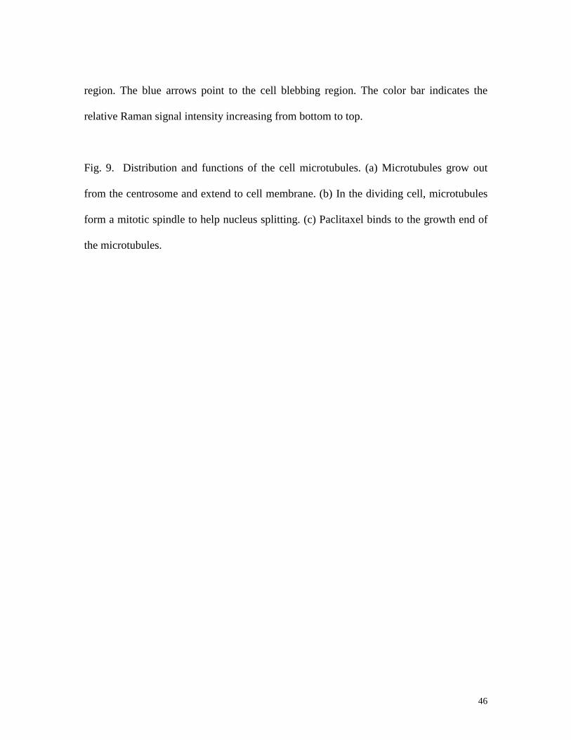
Fig. 9. Distribution and functions of the cell microtubules. (a) Microtubules grow out

from the centrosome and extend to cell membrane. (b) In the dividing cell, microtubules

form a mitotic spindle to help nucleus splitting. (c) Paclitaxel binds to the growth end of

the microtubules.