DIRECT STATISTICAL MATHIMATICAL CALCULATIONS OF FULL ...

IEEE NPSS (Toronto), UOIT, Oshawa, ON, 2-3 June, 2011

International Workshop on Real Time Measurement, Instrumentation & Control [RTMIC]

P210-1

DIRECT STATISTICAL MATHIMATICAL MODEL TO CALCULATE THE

FULL ENERGY PEAK EFFICIENCY OF HPGe DETECTOR

Younis S.Selima, Mohamed S. Hussiena,b, Mohamed A. Fawzya, Ahmed M. El khatibea

a Department of Physics, Faculty of Science, Baghdad St., Moharrum Bey, Alexandria 21511, Egypt.

b Department of Chemistry & Chemical Engineering, Royal Military College of Canada P.O. Box 17000, Station Forces, Kingston, Ontario,K7K 7B4

E-mail: [email protected]

Keywords: gamma spectroscopy systems; HPGe detector efficiency; full energy peak efficiency; photopeak coefficient; direct statistical mathematical model

Abstract

A direct statistical mathematical model was implemented to calculate

the full energy peak efficiency (FEPE) of HPGe detectors over gamma ray

energy range of 20 keV to 3 MeV. This mathematical model can be applied at

any height from the detector face of an axial point source. The idea of the

model depends of on tracking of successive interactions of gamma ray

photons in the energy range under consideration and uses the physics of

these interactions with the geometry information to calculate the photo peak

attenuation coefficient , and consequently the photo peak efficiency .

All calculations were carried out for different cylindrical detector sizes

over distances of 0 to 25 cm from the detector face of the axial point source.

The relative efficiencies of different sizes of HPGe detectors to NaI detectors

that were calculated by the present model have an excellent agreement with

published work.

The calculations of FEPE carried out by the present model were

compared with results from other methods such as experimental, semi

empirical and Monte Carlo calculations. The results of the present model are

in excellent agreement with published FEPE results from these methods, and

provide the best match of experimental results than other theoretical methods.

(1) Introduction

Gamma spectrometry is one of the tools commonly used for the

measurement of various environmental radionuclides. Where, the absolute

activity of different gamma peaks in a wide energy range can be determined,

mailto:[email protected]



P210-2

Gamma ray radioactive isotopes can be identified, measuring the absorbed

doses and determination of the interaction cross sections.

To calculate the absolute activity, the sample to detector full-energy

peak efficiency should be known. The calculation of sample to detector full-

energy peak efficiency using semi-empirical, Monte Carlo approaches and

experimental measurements have been treated by several authors. The semi-

empirical method has been used by Hoste [1], Moens et al. [2] , Lippert [3]

,Mihaljevic et al. [4], Wang et al.,[5] and Wang et al., [6] . In this method, the

full-energy peak efficiency is calculated by combining point source

measurements with computer calculations using empirical formulae. It

involves some approximations and simplifications so the application is

restricted to limited source–detector configurations. While Wainio and Knoll

[7], and Overwater et al. [8] and B.Lal et al. [9] used Monte Carlo method in

which, the history of each individual photon, is simulated in an analog step-by-

step process in the detector active zone. There are no approximations or

limitations to the source–detector configurations, but it is computationally time

consuming more discussions about these two theoretical methods are found

in Ref. [1,…17]. On the other hand the experimental method has been used to

calculate FEPE by T.Paradellis et al. [18] and A.Owens [19]. The relative

advantages and disadvantages of each of this methods are discussed in

[1,…19].

The aim of this work is introducing a new direct mathematical Model to

calculate full energy peak efficiency of cylindrical HPGe detector for an axial

point sources emitting photon of energies up to 3 MeV. To calculate the FEPE

(εp) the photopeak coefficient (μp) must be calculated accurately that could be

achieved through the direct statistical calculation and using spherical

trigonometry technique. This technique based on the determination of the

average path length covered by a photon inside the detector active

medium and the geometrical solid angle (Ω) which represent the angle

subtended by the detector at the source point.

The arrangement of this paper is as follows. Sections (2) and

(3) present direct statistical mathematical formulae for the total efficiency and

peak efficiency for axial point source. Sections (4) and (5) cover the

definitions and calculations of full energy peak attenuation coefficient (μp) and

http://www.sciencedirect.com/science?_ob=ArticleURL&_udi=B6TJ0-4KGPP93-1&_user=2620289&_coverDate=12%2F31%2F2006&_alid=1746105699&_rdoc=5&_fmt=high&_orig=search&_origin=search&_zone=rslt_list_item&_cdi=5296&_sort=r&_st=13&_docanchor=&view=c&_ct=21&_acct=C000058183&_version=1&_urlVersion=0&_userid=2620289&md5=fe3684ed489dbd95254aac84df547b78&searchtype=a#bib6







P210-3

partial attenuation factor (fm). Sections (6) and (7) enclose the method of

calculations of both average scattered energies and the average cosine angle

of scattering respectively. Section (8) contains the longitudinal and lateral

limitation of the scattered ray in the finite detector medium. Section (9)

presents an example of calculating full energy peak efficiency, comparisons

between the calculated peak efficiency using the formulae derived in this work

and the published results that proving the validity of the present mathematical

formulae. Finally, the Conclusion is presented in Section (10).

(2) The direct statistical mathematical method

The direct statistical mathematical approach, present work, provides one

of the simplest, potentially and most accurate methods for predicting the

FEPE. Selim and Abbas [20,21,22] derived mathematical expressions to be

used directly by the substitution of geometrical parameters of the source-

detector system and the total attenuation coefficient (μ) of the incident photon

corresponding to its energy (Eγ) to find the total efficiency, for any source

shape, for any cylindrical detector and at any geometrical locations. The idea

of this method is illustrated in Ref. [20], where the total attenuation coefficient

(μ) is the summation of all the coefficients that attribute to consideration

efficiency μ=τ+σ+. Selim and Abbas formula (1) is used for different source

shape at different places with respect to cylindrical detector. In this work, we

interested in full energy peak efficiency for the axial point source so that the

total attenuation coefficient (μ) will be replaced with the photopeak coefficient

(μp) which calculated accurately through new technique discussed in some

details in the following sections.

(3) Axial Point Source

By using spherical coordinate, the integration limits change in steps in

accordance to the values of the effective traversed distance and the polar

angle (θ). The geometry of coaxial point source to the cylindrical detector

(2R×L) is given in figure (1).

Figure (1): The geometry of coaxial

point source to the

cylindrical detector (2R×L) L

θ2

h

θ1

Axial point source



P210-4

Therefore the total efficiency (T) can be expressed as

(1) (1)

Where;

(2)

Equation (1) is applied to calculate the total efficiency due to an axial point

source to a bare detector. The most germanium detectors use a thin cap

window so the attenuation of this window must to be taken under

consideration. For capped detector the equation (1) multiplied by θ cos

tμ t

e

and

becomes

(3)

Where;

μ: is the total attenuation coefficient of the detector material;

L: is the detector height

R: is the radius of detector face

h: is the distance between the source and the detector face

t: is the window thickness, and

(4)

(μt) is the total attenuation coefficient of the window material which is usually

Aluminum unless stated. If there is n-number of caps or shield we multiply the

where; (μtn) is the coefficient of the nth. element; And, (tn) is the thickness of

nth. element. The dead distance (ho), the distance between the detector active

medium and the window, has to be added to (h) for the source –detector

separation distance.

(4) Full Energy Peak Attenuation Coefficient (μp)

The full energy peak efficiencies defined as the ratio between the number

of photons that are recorded in the detector under certain peak and the

1 2

10

cossincos sin1 sin12

1θ θ

θ

θ

μh

θ

μR

θ

μL

T dθedθeε

1 2

10

cossin coscos cos sin1 sin12

1θ θ

θ

θ

μh

θ

μRt

θ

μLt

T dθeedθeeεtt

θ cos

tμ

θ cos

tμ

θ cos

tμnnt

22t

11t

eee

h

R

Lh

Rθ

1

2

1

1

tan

tan



P210-5

number of photons that are emitted from the source with energy relates to this

peak.”

To calculate the full energy peak efficiencies, we consider only the part of

energy deposited in the detector and which only contributes to the peak, say

photopeak attenuation coefficient (μp) then, the total attenuation coefficient (µ)

in equation (3) is replaced by the photo peak coefficient (µp) remembering that

the photoelectric effect leads always to electrons of maximum energy, we

have to consider the incident gamma rays energies is less than 3 MeV; So

that the coefficient (μp) given by;

(5) where, m=1,2,…..

(τo) is the photoelectric coefficient,

(σo )is the Compton scattering coefficients and

(fm) is a fraction allowing for successive Compton scattering .

Where, the final scattered photon after Compton scattering is terminated by a

photoelectric absorption. This fraction is primarily depends on the detectors

dimensions and incident gamma ray energy.

The index (m) is integer numbers 1,2, ..Confining ourselves to gamma ray

energy less than about 3 MeV; we take only these two terms where the

probability of pair production in this energy range is very small. One of the

main objects of this work is the determination of the fraction (fm) with respect

to the detector’s dimensions, which will maintain in next section.

(5) The Partial Attenuation factor (fm)

Infinite Size Ge detector:-

In order to fully understand the exact behavior of the factor (fm) in the

attenuation coefficient, We preferably start with an infinite size detector with

interacting gamma-rays energy hνo less than 3 MeV where the major

predominant interactions Photoelectric interaction and Compton scattering.

So, we have only two possible allowances to be followed:-

Photoelectric interaction (τo): where, an electron produces in the detector

medium with a kinetic energy equal (hν0-B.E.), thus, being recorded under

the peak energy spectrum.

omop f



P210-6

Compton interaction (σo): The result of which is an electron set in motion with

a kinetic energy To and a scattered photon with energy hν1

hν1 = hνo – To (6)

Consequently; the last scattered photon has one of two fates:-

First fate; a photoelectric effect takes place, thus, an electron with a kinetic

energy equal to (hν1-B.E.) is set in motion.

Now, this electron and the previous scattered one; take place in rapid

succession that they appear as one electron with a total energy hνo that is

registered at the maximum peak position of the detector. The relative

probability of this to happen is:-

(7)

μ1 the total attenuation coefficients of the scattered gamma rays with energy

hν1.

Second fate; If the previous interaction does not take place, the rest

fraction of the original beam σ1/μ1 propagates, and will be scattered to an

electron with a kinetic energy T1 and a scattered gamma ray with energy

hν2. Letting this last scattered photon undergoes a photoelectric effect

with a probability

2

2

μ

τ. These three electrons are again emitted promptly

and they appear as one with a total kinetic energy equals to original

energy of incident ray hνo, Since range of the electrons is few microns

only up to about a millimeter thus appear again in the photo-peak region.

The relative probability of this to happen is:

2

2

1

1

μ

τ .

μ

σ

Of course, only one event of either of the two fates takes place. Then the

average probability will be:-

(8)

Therefore; for an infinite medium and allowing for further Compton scattering;

the average effective fraction of the Compton components is given by:-

(9)

2

2

1

1

1

12 ..

2

1

f

,...3,2,1;..1

1

1

3

3

2

2

1

1

2

2

1

1

1

1

mm

fm

m

m

mm

1

1

1

ffm



P210-7

Where, m is a total number of effective collisions.

Using equations (5,9) and tables in (24) one can calculate the photopeak

efficiency for relation (3) after substituting total attenuation coefficient (µ) with

photopeak coefficient µp then the photopeak efficiency given by for axial point

source.

(10)

Now, the problem is calculating the partial coefficient corresponding to the

energies of scattered photons τ1 , τ2 τ3….. τm and σ1, σ2, σ3, …..σm-1. So, the

average scattered energies should be calculated.

(6) Calculation of Average Scattered Energies

In order to find the partial attenuation fractions, we have to determine

the scattered energies of the gamma rays. A statistical process governs this

phenomenon, similar to neutron scattering process. Beforehand, the

kinematics of the interaction is controlled by the famous Compton’s set of

equations. According to Compton scattering this interaction, as the photon

falls with energy (hνo), its momentum is (hνo/c). From the conservation of

momentum, where the scattering is elastic, the scattered photon must be

changed from the incidence direction by angle (θ) and the electron removes

with angle (υ) but the three directions, the incidence, the scattered and the

remove recoil must lie in the same plane i.e. un-polarized scattered radiation

is considered.

From the conservation of energy, the photon loses part of its energy, which

the electron acquires as a kinetic energy.

Energy of the scattered photon is given by:

(11)

(12)

The energy expectation value of the average energy for the scattered photon

is

(13)

ohFh .1

θ)(

hνhν o

cos11 1

2.cm

hν

e

o

dd

d

dd

dh

ho

o

1

1

1 2

10

cossin coscos cos sin1 sin12

1θ θ

θ

θ

hμ

θ

Rμt

θ

Lμt

p dθeedθeeεpptpt



P210-8

(14)

where,

(14)

In order to calculate the average scattered photon energy, it is required to

know the angular distribution of the scattered photon to determine the

deposited energy. So, The probability of Compton scattering at the angle (θ)

can be determined through quantum mechanical calculation of the process.

Klein and Nishina [25] derived a formula for the angular distribution to the un-

polarized scattered radiation as:-

(15)

To calculate the expected scattered photon energy < hν1>, we integrate the

values of hν1 over all the possible angles θ.

(16)

where;

(17)

Using equations (13,14,15,16) and (17). The reduction factor (F) given by

(18)

By, Carrying out the integration of the different factors term by term of

equation (18) the reduction factor (F) of the original energy leading to

averaged energy for the scattered beam or photon in any medium, could be

expressed as:-

dd sin2

π

π

o

dθθ)(

θf

dθθ)(

θ θfh

hν

0

2

0

3

1

cos11

sin

cos11

sin

π

π

o θ d( θ

θ(θ

θ

θ d( θ

θ(θ

θ

hν

hνF

0

222

2

0

222

3

1

)cos)cos1( 1

)cos1cos1

) cos(1 1

1

)cos)cos1( 1

)cos1cos1

) cos(1 1

1

)cos1(1

)cos1(cos1)(

222

f

)cos1(1

) cos1(cos1

) cos1(1

1

2

222

2

2

oo r

d

d



P210-9

416182)21ln(]22[)21()21(3

630361232)21ln()21(323423

23453

F (19)

Where, () is stated as before in equation (12). Figure (2) indicates the

variation of reduction factor (F) with the photon energy (hν). It is important to

notice that, for higher energies of the incident gamma rays the sharp

reduction of energies is more than that for the incident lower energies.

(7) Calculation of The Average Cosine Angle Of Scattering

The average cosine angle of the scattered photon is given by

(20)

Where; dΩ

dσo as is defined in equation (15) therefore

(21)

π

o

π

o

dΩdΩ

dσ

dΩdΩ

dσθ

θ

0

0

cos

cos

π

0

22

2

2

π

0

22

2

3

dθsinθθ) cos(11

θ) cos(1αθcos1

θ) cos(11

1

dθsinθθ) cos(11

θ) cos(1θcos1

θ) cos(11

θ cos

cosθ

Figure (2): The variation of reduction factor F with the photon

energy hν

Figure (3): The variation of

average cosine <cos θ> with (hν)



P210-10

By solving these two integrations, Carrying out the integration term by term,

we finally get;

416182)21ln()22()21(

63046166)21ln()36()21( cos

23422

2345232

(22)

Where () is as defined before in equation (12). One can notice that, the

average cosine depends also on the incident photon energy. The variations of

<cos θ> with the photon energy (hν) is presented in figures (3) where the

energetic gamma rays (MeVs’) are scattered forwards, while softer rays

(KeVs’) are scattered sideward. The correlated understanding between

Figures (2) and (3) can be explained as when an incident photon with

relatively high energy is scattered then much of its energy is reduced i.e. (F)

becomes small and penetrates more forward i.e. (θ) is small then <cos θ>

becomes big till the photon energy is much reduced and the situation is

interchanged. For smaller energies, the energy reduced more slowly i.e. (F)

becomes big and tend to be lose to 1 and spreads more side–wards i.e. (θ)

increases.

By using equation (13) for every incident gamma energy (hνo ) , the

average energies of the successive Compton-scattered rays <hν1> , <hν2>

,…. could be deduced. From table (1) and equations (9,13 and 18) and data

from tables [24] the components of the partial attenuation coefficient could be

computed

(23)

m

m

m

m

1

1

3

3

2

2

1

1

2

2

1

1

1

1 .,,.,



P210-11

Figure (4) shows the variation of coefficients (μ, μp and τo) with the photon

energy for infinite size germanium detector. One can notice that the difference

between (μp) and (τo) at high energy explain the feasibility of this work.

The partial attenuation coefficient in expression (23) consider the infinite

number of scattering or successive interactions that could be happened only

in the infinite detector medium but actually the detection medium is finite so

the longitudinal and lateral limitation should be considered.

(8) Finite Size Ge Detector

In this case, we consider the assumption that all electrons from the

photoelectric effect or/and Compton scattering are completely absorbed within

the detector volume. Since range of the electrons is few microns only up to

about a millimeter. Therefore, the photoelectric coefficient (τo) would not be

affected. Only Compton-components affected because of the scattered

gamma ray photons that may be escape before absorption in the detector

medium and contributing to previous mentioned coefficient (ƒm). So the

longitudinal and lateral limitation should be considered to determine the

limitation number of (m) successive scattering.

(8-a) Longitudinal Limitation

Let a gamma ray of energy (hνo) to be incident axially and normally to

the detector’s surface. Its path length is (L). The absorption probability in the

detector is:-

(24) LLL oo eee

.0

Figure (4): Variation of total attenuation, peak, and photoelectric Coefficients with the photon energy for an infinite Germanium detector



P210-12

The mean free path of the photoelectric effect is (1/τo); and that of Compton

scattering for the first elastic collusion is (1/σo). The average energy of the

scattered photon becomes (hν1) with a scattering angle (1).

Figure (5) illustrates the mean free paths and the scattering angles for

successive scattered photon inside the cylindrical detector of dimension

(2R×L). The component in the direction of incidence is clearly

(25)

Further, let this ray be scattered further to let its energy be hν2 with a space

scattering θ2 making an angle (β) with the original direction of incidence and a

rotation angle υ2, where υ2 is the angle of rotation of the third mean free path

with respect to the plane of the first two paths.

Following the same steps as followed by [25] for the scattering of neutrons

(26)

Since all values of (υ2) are equally probable for un-polarized rays, then the

average value of the second term in the last equation is zero. Accordingly,

(27) 12

2

2 .cos cos .1

x

22121 cos.sin.sincos.coscos

1

1

1 cos1

x

Figure (5): The mean free paths and the scattering angles for successive scattered photon inside the cylindrical detector of dimension (2R×L).



P210-13

And so on, for further scatterings. One condition to determine the suitable

value of index number (m) in the fraction (ƒm) is

m1

m

21

2

1

1o

cos cosσ

1 cos cos

σ

1 cos

σ

1

σ

1L (28)

In effect, for an axial isotropic point source being situated at a distance (h)

from the detector’s surface the average photons ray may not fall normally on

the detector surface.

Therefore, the gamma ray photons may be inter to the detector medium from

any point on the upper surface with equally probability, so the average

covered path of a ray is not (L) but ( ) as shown in the sketch figure (6).

The average covered distance of a ray from an axial point source at height

(h) from the detector surface could be calculated. The allowed photon

distance ( ) is the average distance which represents a straight line

connecting the photon incident point on the detector and the photon outgoing

point from the detector. Therefore ( ) is considered as a function in solid

angle and due to the statistical nature of the radiation, the allowed photon

distance ( ) can be expressed, form of isotropic emission by formula

Figure (6): The average covered distance of a ray from an axial point source at distance (h) from the upper detector face



P210-14

This integration is divided into two parts each of them is depending on the

variation of ( ) with (θ1) and (θ2)

Where,

So from figure (6) and equations (29, 30 and 31) the average covered path

could be given by equation (32).

22

2222

11

1

)(ln).(ln.

)(tantan

Rh

h

RLh

hLLh

Rh

hh

Lh

R

h

RR

d (32)

By plotting this average path distance ( ) with the source height distance (h)

for different detector dimensions (2RxL) or volumes sizes as shown in figure

(7) one can conclude that

a) For axial point source, just on the detector face, the average path

distance covered in the detector is increase by increase the detector

volume.

(

Figure (7): The variation of the average covered path with the source height for different detector volumes with dimensions (2RΧL)



P210-15

b) As the height (h) increase the average distance start to decrees until

minimum value. This minimum values of is depend on the detector

volume and height of the source so the significant conclusion of the

minimum average distance of the gamma ray photon in the detector is

correlated with the distance of the source from the detector face and the

volume of the detector. Then, by replacing (L) in equation (28) with ( ) the

longitudinal limitation becomes:-

(33)

(8-b) -Lateral Limitation

The other condition for the maximum value of (m) to be considered for

contributing to eligible successive Compton scatterings is the so-called lateral

condition. Namely, for an axial ray falling along the detector’s axis i.e. the ray

enter from the central point of the upper detector face, it is straight forward to

get:-

(34)

In fact, considering the effective averaged ray entering the detector from any

point of the upper detector circular face, then the initial entering lateral

distance or entrance angle (θ0) should be considered as shown in figure (8-a)

and the lateral condition becomes:

).....sin(.1

.......)sin(.1

)sin.1

tan.( 2010

1

0

0

0 m

m

hR

(35)

Where, (θo) is the angle of incidence of the averaged ray in the detector. It is

computed from the relation:

(36)

The initial angle of scattering (θo) can be calculated graphically as shown in

fig. (8)

).....sin(1

)sin(1

sin1

2121

2

1

1

m

m

R

sincos 00

Rhd

m1

m

21

2

1

1o

θ cosθ cosσ

1θ cosθ cos

σ

1θ cos

σ

1

σ

1d



P210-16

After (fm) is calculated the photopeak coefficient can be calculated from

(37)

(9) Results (9-1)Calculating Photo Peak Efficiency at Discreet Gamma Energy

Table(1) reproduces the peak coefficient (μp) for a finite size Ge

detector, allowing for (m) successive Compton collision. The first column is

the energy of gamma rays in MeV. The second represents the photoelectric

coefficient alone (τo). The third column gives the values of (μp) for the case

m=1 to m=6. All units are in cm-1. In practice for customary detectors, the

column m=1 is to be taken for low energies till about 0.3 MeV, while values of

m=2 and 3 are used for higher energies.

omop f

Figure (8-b): calculating the initial

angle of scattering θo graphically Figure (8-a): calculating lateral

limitation condition



P210-17

Figures (9a and 9b) are showing the variation of the photopeak attenuation

coefficient with number of successive scatterings at different energy for infinite

detector size (Ge-Detector). From these figures one can conclude that at

small energies the photo peak coefficient (μp) is come to maximum after first

or second collision where the photons interactions terminated by photoelectric

interaction. But, as the gamma ray energy going up photo peak coefficient (μp)

increases gradually and reaches to maximum after 4; 5 or 6 successive

collisions. Since these graphs for infinite detector medium then one can notice

the number of collisions until 13. But, in real conditions the number of

successive collisions or scattering are limited by escape from the finite

detection medium or, terminated by photoelectric absorption.

Table (1): The peak coefficient μp for a finite size Ge detector, allowing for (m) successive Compton collision.

hv (MeV) τo

μp

m=1 m=2 m=3 m=4 m=5 m=6

0.015 481.1992 482.467 482.2300 482.1507 482.1110 482.087 482.071

0.020 220.3722 220.911 220.6423 220.5523 220.5073 220.480 220.462

0.030 71.3282 74.5888 74.2911 74.1907 74.1404 74.1103 74.0902

0.040 31.0863 31.7043 31.3998 31.2954 31.2431 31.2118 31.1908

0.050 16.1819 16.7999 16.4995 16.3938 16.3408 16.3090 16.2878

0.060 9.4749 10.0748 9.7886 9.6844 9.6321 9.6006 9.5797

0.080 4.0029 4.5625 4.3073 4.2070 4.1560 4.1254 4.1050

0.100 2.0440 2.5401 2.3315 2.2386 2.1901 2.1609 2.1414

0.150 0.5962 0.9723 0.8423 0.7699 0.7277 0.7015 0.6840

0.200 0.2518 0.4944 0.4527 0.4036 0.3691 0.3461 0.3304

0.300 0.0767 0.2057 0.2059 0.1934 0.1735 0.1561 0.1432

0.400 0.0341 0.1124 0.1201 0.1219 0.1152 0.1033 0.0927

0.500 0.0188 0.0644 0.0824 0.0895 0.0878 0.0804 0.0717

0.600 0.0119 0.0430 0.0598 0.0675 0.0700 0.0669 0.0601

0.800 0.0061 0.0230 0.0329 0.0452 0.0517 0.0521 0.0480

1.000 0.0038 0.0144 0.0224 0.0334 0.0399 0.0417 0.0402

1.250 0.002433 0.0095 0.0145 0.0231 0.0300 0.0340 0.0340

1.500 0.001751 0.0067 0.0107 0.0166 0.0241 0.0287 0.0297

2.000 0.0011 0.0040 0.0065 0.0111 0.0177 0.0220 0.0235

3.000 0.0006 0.0020 0.0034 0.0058 0.0101 0.0140 0.0165



P210-18

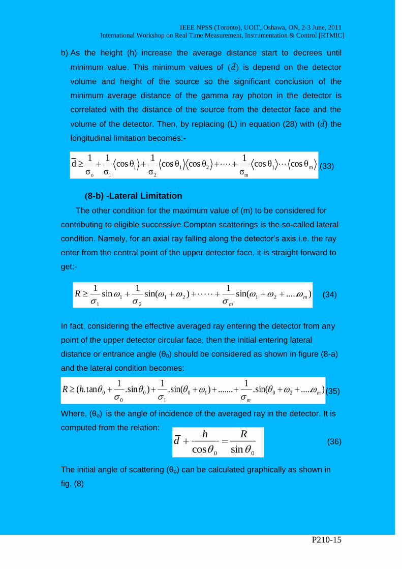
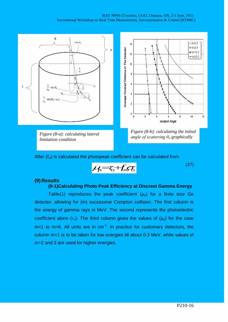
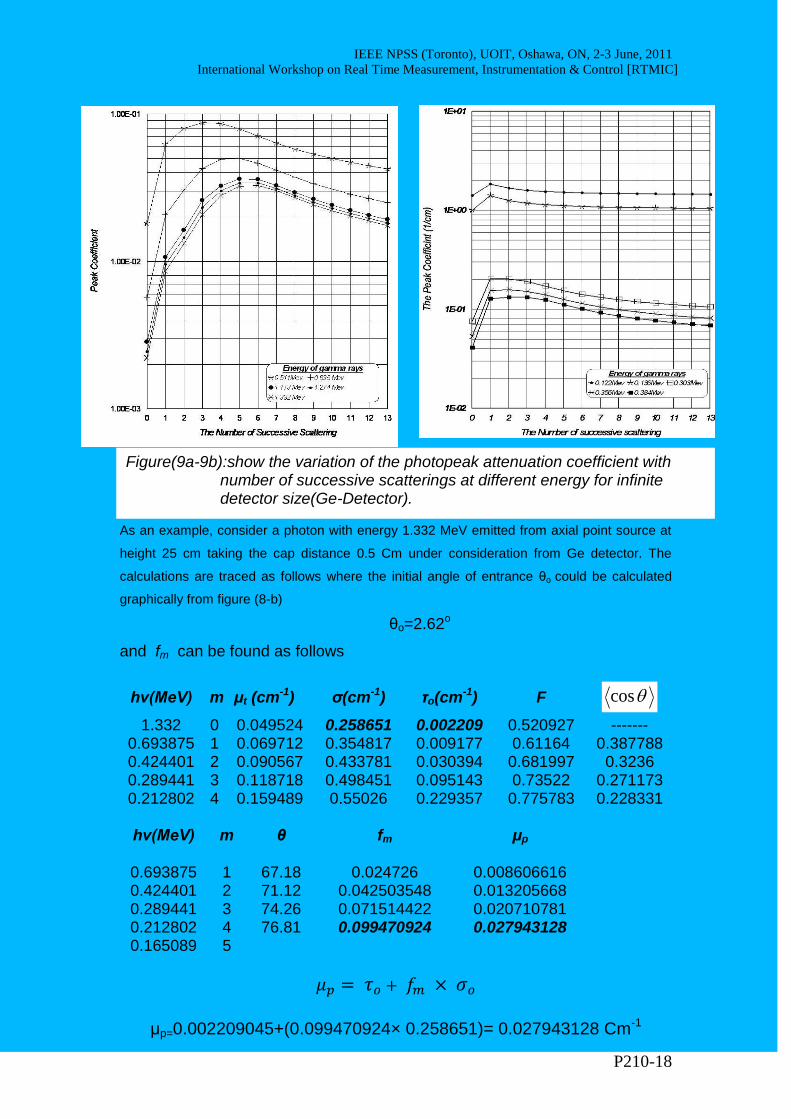
Figure(9a-9b):show the variation of the photopeak attenuation coefficient with number of successive scatterings at different energy for infinite detector size(Ge-Detector).

As an example, consider a photon with energy 1.332 MeV emitted from axial point source at

height 25 cm taking the cap distance 0.5 Cm under consideration from Ge detector. The

calculations are traced as follows where the initial angle of entrance θo could be calculated

graphically from figure (8-b)

θo=2.62o

and fm can be found as follows

hν(MeV) m μt (cm-1) σ(cm-1) τo(cm-1) F cos

1.332 0 0.049524 0.258651 0.002209 0.520927 ------- 0.693875 1 0.069712 0.354817 0.009177 0.61164 0.387788 0.424401 2 0.090567 0.433781 0.030394 0.681997 0.3236 0.289441 3 0.118718 0.498451 0.095143 0.73522 0.271173 0.212802 4 0.159489 0.55026 0.229357 0.775783 0.228331

hν(MeV) m θ fm μp

0.693875 1 67.18 0.024726 0.008606616 0.424401 2 71.12 0.042503548 0.013205668 0.289441 3 74.26 0.071514422 0.020710781 0.212802 4 76.81 0.099470924 0.027943128 0.165089 5

μp=0.002209045+(0.099470924× 0.258651)= 0.027943128 Cm-1



P210-19

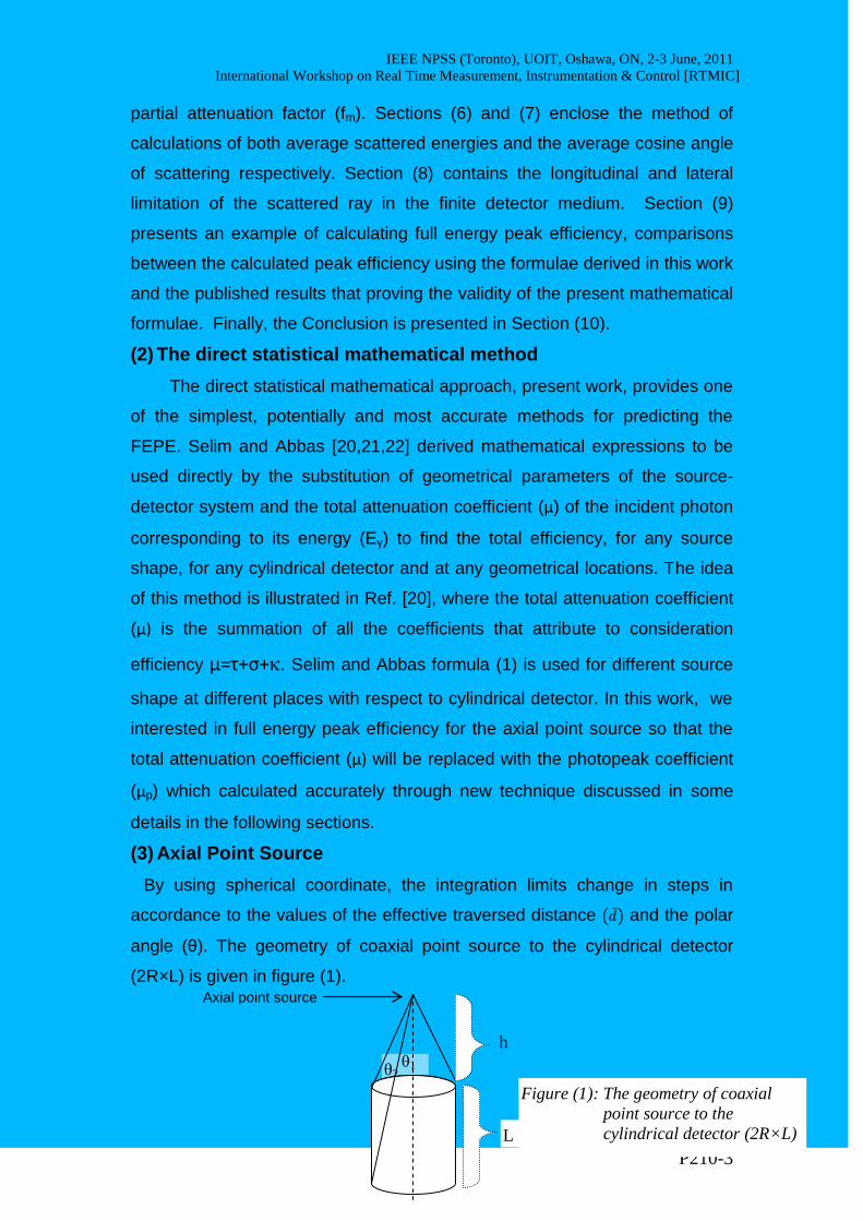
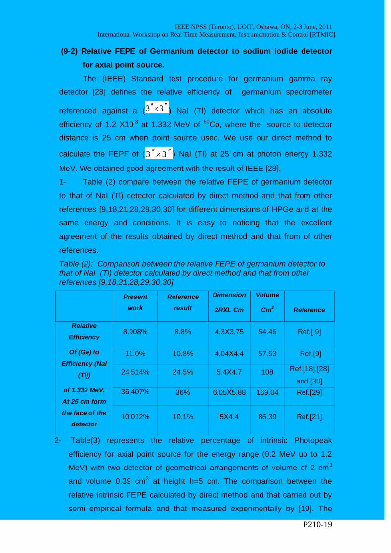
(9-2) Relative FEPE of Germanium detector to sodium iodide detector

for axial point source.

The (IEEE) Standard test procedure for germanium gamma ray

detector [28] defines the relative efficiency of germanium spectrometer

referenced against a ( 33 ) NaI (Tl) detector which has an absolute

efficiency of 1.2 X10-3 at 1.332 MeV of 60Co, where the source to detector

distance is 25 cm when point source used. We use our direct method to

calculate the FEPF of ( 33 ) NaI (Tl) at 25 cm at photon energy 1.332

MeV. We obtained good agreement with the result of IEEE [28].

1- Table (2) compare between the relative FEPE of germanium detector

to that of NaI (Tl) detector calculated by direct method and that from other

references [9,18,21,28,29,30,30] for different dimensions of HPGe and at the

same energy and conditions. It is easy to noticing that the excellent

agreement of the results obtained by direct method and that from of other

references.

2- Table(3) represents the relative percentage of intrinsic Photopeak

efficiency for axial point source for the energy range (0.2 MeV up to 1.2

MeV) with two detector of geometrical arrangements of volume of 2 cm3

and volume 0.39 cm3 at height h=5 cm. The comparison between the

relative intrinsic FEPE calculated by direct method and that carried out by

semi empirical formula and that measured experimentally by [19]. The

Table (2): Comparison between the relative FEPE of germanium detector to that of NaI (Tl) detector calculated by direct method and that from other references [9,18,21,28,29,30,30]

Present

work

Reference

result

Dimension

2RΧL Cm

Volume

Cm3

Reference

Relative

Efficiency

Of (Ge) to

Efficiency (NaI

(Tl))

of 1.332 MeV.

At 25 cm form

the face of the

detector

8.908% 8.8% 4.3Χ3.75 54.46 Ref.[ 9]

11.0% 10.8% 4.04Χ4.4 57.53 Ref.[9]

24.514% 24.5% 5.4Χ4.7 108 Ref.[18],[28]

and [30]

36.407% 36% 6.05Χ5.88 169.04 Ref.[29]

10.012% 10.1% 5Χ4.4 86.39 Ref.[21]



P210-20

agreement between these results is very good through the energy range

under consideration.

Table (3): The comparison between the relative intrinsic FEPE calculated by direct method and that carried out by semi empirical formula and measured experimentally by [19].

Detector Volume (Cm

3)

Photon Energy

(MeV)

Relative Intrinsic Efficiency [19]

Direct Method (Present

Work) Experiment-

ally Calculated by

Semi-empirical

2.0

0.2 20.5Χ0.9 21.0 20.2908

0.3 8.0 Χ 0.6 8.10 8.5258 0.5 2.55 Χ 0.09 2.60 2.9303 0.8 1.1 Χ 0.05 1.09 1.0566

1.00 0.76 Χ 0.04 0.76 0.6631 1.2 0.56 Χ 0.02 0.55 0.4844

0.39

0.2 26.0 Χ 2.0 27.20 20.0778 0.3 8.6 Χ 0.4 9.00 8.9415 0.5 2.50 Χ 0.40 2.45 2.8968 0.8 0.87 Χ 0.05 0.88 1.0444

1.00 0.56 Χ 0.08 0.58 0.6555 1.2 0.39 Χ 0.07 0.41 0.4788

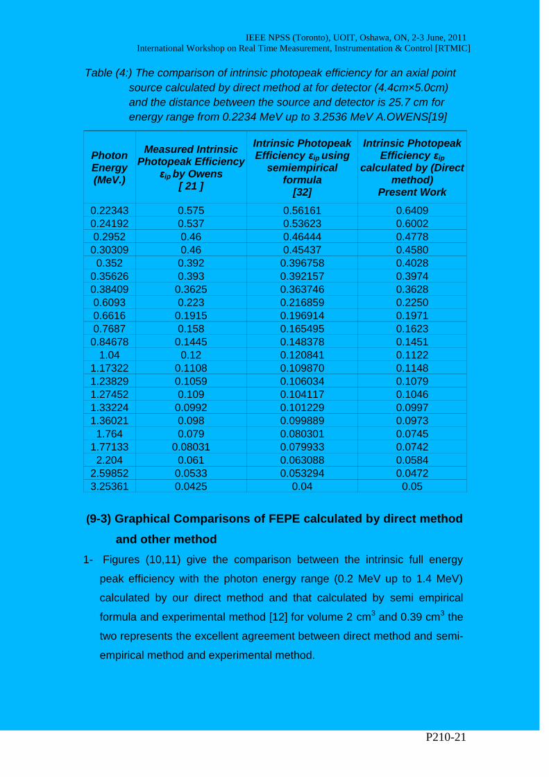
3- Table (4) gives the comparison of intrinsic photopeak efficiency for an axial

point source calculated by direct method at for detector (4.4cm×5.0cm) and

the distance between the source and detector is 25.7 cm for energy range

from 0.2234 MeV up to 3.2536 MeV A.OWENS [19] that measure the

FEPE experimentally and also compared with the result carried out by

HAJNAL and KLUSEK [30] that use semi empirical method. One can see

that the agreement of direct method results with the experimental and

semiempirical results is very good.



P210-21

Table (4:) The comparison of intrinsic photopeak efficiency for an axial point

source calculated by direct method at for detector (4.4cm×5.0cm)

and the distance between the source and detector is 25.7 cm for

energy range from 0.2234 MeV up to 3.2536 MeV A.OWENS[19]

Photon Energy (MeV.)

Measured Intrinsic Photopeak Efficiency

εip by Owens [ 21 ]

Intrinsic Photopeak Efficiency εip using

semiempirical formula

[32]

Intrinsic Photopeak Efficiency εip

calculated by (Direct method)

Present Work

0.22343 0.575 0.56161 0.6409

0.24192 0.537 0.53623 0.6002

0.2952 0.46 0.46444 0.4778

0.30309 0.46 0.45437 0.4580

0.352 0.392 0.396758 0.4028

0.35626 0.393 0.392157 0.3974

0.38409 0.3625 0.363746 0.3628

0.6093 0.223 0.216859 0.2250

0.6616 0.1915 0.196914 0.1971

0.7687 0.158 0.165495 0.1623

0.84678 0.1445 0.148378 0.1451

1.04 0.12 0.120841 0.1122

1.17322 0.1108 0.109870 0.1148

1.23829 0.1059 0.106034 0.1079

1.27452 0.109 0.104117 0.1046

1.33224 0.0992 0.101229 0.0997

1.36021 0.098 0.099889 0.0973

1.764 0.079 0.080301 0.0745

1.77133 0.08031 0.079933 0.0742

2.204 0.061 0.063088 0.0584

2.59852 0.0533 0.053294 0.0472

3.25361 0.0425 0.04 0.05

(9-3) Graphical Comparisons of FEPE calculated by direct method

and other method

1- Figures (10,11) give the comparison between the intrinsic full energy

peak efficiency with the photon energy range (0.2 MeV up to 1.4 MeV)

calculated by our direct method and that calculated by semi empirical

formula and experimental method [12] for volume 2 cm3 and 0.39 cm3 the

two represents the excellent agreement between direct method and semi-

empirical method and experimental method.



P210-22

Figure (12) present Comparison of variations of Full Energy Peak Efficiency

for the energy range from 0.1 MeV and 2.5 MeV. These comparison were

carried out between the present Direct Method and, that calculation by

WAINIO and KNOLL, ref [7], that using Monte Carlo calculation by B.LAL et

al. ref.[9] and by experimental value of CLINE ref. [31] for detector dimension

of radius R=0.9 cm and depth of L=0.8 cm and the axial point source distance

is 0.8 cm.

Figure (10,11): The comparison between the intrinsic full energy peak efficiency with the photon energy range (0.2 MeV up to 1.4 MeV) calculated by our direct method and that calculated by semi empirical formula and experimental method

Figure (12): Comparison of the Calculated FEPE by direct method and other methods.



P210-23

One can easy notice that the values of the 4-Methods are very closely to

each other but the values calculated by direct method is the closest one to

the experimental measurements compatibility.

(10) Conclusion One can conclude that, an exact mathematical model to calculate

directly photopeak efficiency of HPGe detector with an axial point source at

different distances from the detector surface is derived successfully. The

model is applicable for gamma ray energy range up to 3 MeV where, the

predominant reactions considered are Compton scattering and photoelectric

absorption.

The geometrical and mathematical treatment has been done to

calculate the average path of the gamma ray in the detector and consequently

its the lateral and longitudinal limitations in the finite detector size.

Consequently,

The term photo peak coefficient was calculated accurately.

The full energy photo peak efficiencies calculated by direct

mathematical model, for different detector sizes, found in an excellent

agreement with other accurate published works by other methods and more

closer to experimental measurements than other theoretical calculations.

Finally, one can say that this work gives a good support and enhance

calculations of absolute activity of γ-sources with different geometry in

addition to improving the calibration of HPGe detectors.



P210-24

(11) References

[1] Hoste, 1981 J. Hoste, Calculation of the absolute peak efficiency of gamma-ray detectors for different counting geometries, Nucl. Instrum. Methods 187(1981), p. 451.

[2] Moens et al., 1983 L. Moens and J. De Donder et al., Calculation of the peak efficiency of high-purity germanium detectors, Int. J. Appl. Radiat. Isot. 34(1983), p. 1085.

[3] Lippert, 1983 J. Lippert, Detector-efficiency calculation based on point-source measurement,

[4] Mihaljevic et al., 1993 N. Mihaljevic and S. De Corte et al., J. Radioanal. Nucl. Chem. 169 (1993), p. 209.

[5] Wang et al., 1995 T.K. Wang and W.Y. Mar et al., HPGe detector absolute-peak-efficiency calibration by using the ESOLAN program, Appl. Radiat. Isot. 46(1995), p. 933.

[6] Wang et al., 1997 T.K. Wang and W.Y. Mar et al., HPGe detector efficiency calibration for extended cylinder and Marinelli-beaker sources using the ESOLAN program, Appl. Radiat. Isot. 48 (1997), p. 83.

[7] K. M. Wainio And G.F.Knoll, Nucl. Inst. And Meth. 122 (1966) 213.

[8] Overwater et al., 1993 R.M. Overwater and W.P. Bode et al., Gamma-ray spectroscopy of voluminous sources corrections for source geometry and self-attenuation, Nucl. Instrum. Meth. A 324 (1993), p. 209.

[9] B.Lal and K.V.K.Iyengar (1970) Nucl. Instr. and meth. 79, 19.

[10] Marc Décombaz, Jean-Jacques Gostely and Jean-Pascal Laedermann, (1992) Nucl. Instr. and meth. A312, 152.

[11] Finckh and Geissörfer and et.al (1987) Nucl. Instr. and meth. A262, 441.

[12] G.GAGGERO (1971) Nucl. Instr. and meth. 94, 481.

[13] M.Korun et.al (1997)Nucl. Instr. and meth. A 390, 203.

[14] Gerhard Hasse, David Tait and Arnold Wiechen (1993)Nucl. Instr. and

meth A329,483

[15] H.Seyfarth, A. M. Hassan, B. Hrastnik, P. Gottel W. Delang (1972) Nucl.

Instr. and meth. 105,301

[16] Naim.M.A Isotope & Rad.Res.25,2,65-73(1993)

[17] G.B. Beam, L.Wielopolski , R.P.Gardner, and K.Verghese, (1978) Nucl.

Inst. Method 154,501.

[18] T.Paradellis And S. Hontzeas (1969) Nucl. Instr. and Meth. 73,210

[19] A.Owens (1989) Nucl. Instr. and meth. A(274),297

[20] Selim and Abbas Radiat. Phys. Chem. Vol. 48, No. 1, pp. 23-27, 1996

[21] Y.S. Selim, And M.I. Abbas, M.Fawzy, Rad.Phys.Chem. 53 (1998) 589.

[22] Y.S. Selim, And M.I.Abbas, Rad.Phys.Chem. 58 (2000) 15.

http://www.sciencedirect.com/science?_ob=ArticleURL&_udi=B6TJ0-4KGPP93-1&_user=2620289&_coverDate=12%2F31%2F2006&_alid=1746105699&_rdoc=5&_fmt=high&_orig=search&_origin=search&_zone=rslt_list_item&_cdi=5296&_sort=r&_st=13&_docanchor=&view=c&_ct=21&_acct=C000058183&_version=1&_urlVersion=0&_userid=2620289&md5=fe3684ed489dbd95254aac84df547b78&searchtype=a#bbib10








P210-25

[23] Evans, R.D.(1955) The Atomic Nucleus, Tata McGraw-Hill Press, New

Delhi

[24] Hubbell J.H., Gimm, H.A. (1980) Journal of Physical and Chemical

References Data

[25] Lamarch, J.R. (1960) Introduction to Nuclear Reactor Theory, Addison-

Wesley Press, New York

[26] (IEEE) Standard test procedure for germanium gamma ray detector St,

325-1971.

[27] M.KORUN et.al (1997)Nucl. Instr. and meth. A 390, 203.

[28] Instructional Manual “Aptec Germanium Spectrometer” Type “Coaxial”

Model No. “G220a31gl” Institute Of Higher Studies And Researchs

Alexanderia University.

[29] Hubbell, J.H. And Seltzer S.M. (1995)NISTIR-5623

[30] F.Hajnal And C.Klusek, Nucl. Instr. and Meth. 122(1974)559.

[31] J.E. Cline, IEEE Trans. Nucl. Sci. NS- VOL. 15,No.3 (1968) 198.

Authors 1- Dr. Younis S.Selim,

Prof. Emeritus. of Nuclear Physics

Department of physics , Alexandria University, Egypt

For sorry, He passed away 2007

2- Mr. Mohamed S. Hussien ,

-PhD, Candidate in Royal Military Collage of Canada

-Master of Physics and Technology of Nuclear Reactor Birmingham university, UK, 2008.

-Master of theoretical radiation physics, Alexandria university, Egypt 2003.

Email: [email protected]

3- Dr. Mohamed A. Fawzy,

Prof. of Radiation Physics

Department of physics , Alexandria University, Egypt.


Tel: 002-03- 3911794

4- Dr. Ahmed M. El-Khatib,

Prof. of Experimental Physics

Former hear of the Department of physics, Alexandria University, Egypt.


Tel: 002-03- 3911794





P210-26

Date post:	22-Mar-2022
Category:	Documents
Upload:	others
View:	1 times
Download:	0 times

DIRECT STATISTICAL MATHIMATICAL CALCULATIONS OF FULL ...

Documents