Directionality and Nonlinearity - Challenges in Process...

Directionality and Nonlinearity- Challenges in Process Control

Jonas B. Waller

Academic Dissertation

Process Control Laboratory

Faculty of Chemical Engineering

Abo Akademi University

Abo 2003

Foreword

This thesis has been written at the Process Control Laboratory at the Faculty

of Chemical Engineering at Abo Akademi University. Part of the thesis was

written during the author’s stay as a visiting researcher at the Intelligent

Control Laboratory at the Department of Electrical and Electronic Systems

Engineering at the Graduate School of Information Science and Electrical

Engineering at Kyushu University in Fukuoka, Japan. Overall, the work was

carried out during the years 1993-1994 and 1999-2003.

It has been a painful delivery, indeed. So, in effect, all people I know

have more or less contributed to it. Especially I wish to express my sincere

gratitude to my mentors, foremost my father Professor Kurt Waller and my

supervisor Professor Hannu Toivonen. Their encouragement, support and

truly intelligent comments have been invaluable to me.

Furthermore I wish to thank my colleagues, co-authors and friends;

Dr. Matias Waller, Dr. Jari Boling, Dr. Rasmus Nystrom, Dr. Mats Sagfors

and Bernt Akesson in Finland. Also I wish to express my sincere gratitude

to my friends and colleagues in Japan; Professor Kotaro Hirasawa, Professor

Junichi Murata and Professor Jinglu Hu and the rest of the great people

at the Intelligent Control Lab at Kyushu University. I also wish to express

my gratitude to my colleagues at Abo Akademi University and at Swedish

polytechnic for their encouragement and support.

Also I thank my financial contributors - see the acknowledgements in the

papers. Especially I wish to thank Svenska Tekniska Vetenskapsakademien

i Finland for making it possible for me to perform the latter part of the

research presented in this thesis.

I wish to thank my mother Ann-Christin Waller for her support and for

helping me with the language. Last, but surely not least, I want to thank

my wife Dr. Nari Lee and my lovely daughter Jerin.

i

ii

Abstract

The use of the concepts of directionality and ill-conditionedness is investi-

gated. A lack of consistent terminology is detected, and some clarifications to

the terminology are suggested. Robustness issues with respect to directional-

ity are discussed. Control structures in the form of decoupling are discussed,

and a more general formulation for dynamic decoupling is formulated. Pro-

cess nonlinearity, especially in the form of operating region dependent dynam-

ics, is tackled by the use of a nonlinear input/output model of quasi-ARMAX

type. The model is applied in the model predictive control framework for con-

trol of nonlinear processes, with a pH-process as a case-study. The nonlinear

controller is also reformulated for the multivariable case, and applied to con-

trol of an ill-conditioned, nonlinear distillation column. The computational

demand of the model predictive control formulation is addressed by study-

ing methods to approximate the behaviour of model-predictive controllers by

the use of neural networks as function approximators. Also, as a means to

decrease the online computational demands, a neurodynamic programming

formulation is investigated in the sense that the future cost-to-go function is

calculated by use of offline MPC calculations and then approximated.

iii

iv

List of Publications

This thesis consists of an introductory part and the following papers, referred

to by their roman numerals.

I Defining Directionality: Use of Directionality Measures with Respect to

Scaling, Jonas B. Waller and Kurt V. Waller, Ind. Eng. Chem. Res.,34,

1244-1252, 1995.

II Decoupling Revisited, Matias Waller, Jonas B. Waller and Kurt V.

Waller, Ind. Eng. Chem. Res.,42, 4575-4577, 2003.

III Nonlinear Model Predictive Control Utilizing a Neuro-Fuzzy Predictor,

Jonas B. Waller, Jinglu Hu and Kotaro Hirasawa, Proceedings of IEEE

Conference on Systems, Man and Cybernetics, Nashville, USA, 2000.

IV A Neuro-Fuzzy Model Predictive Controller Applied to a pH-neutral-

ization Process, Jonas B. Waller and Hannu T. Toivonen, Proceed-

ings of IFAC World Congress on Automatic Control, Barcelona, Spain,

2002.

V Multivariable Nonlinear MPC of an Ill-conditioned Distillation Col-

umn, Jonas B. Waller and Jari M. Boling, Submitted to J. Proc. Cont.,

2003.

VI Value Function and Policy Approximation for Nonlinear Control of a

pH-neutralization Process, Jonas B. Waller and Hannu T. Toivonen,

2003.

VII Neural Network Approximation of a Nonlinear Model Predictive Con-

troller Applied to a pH Neutralization Process, Bernt M. Akesson,

Hannu T. Toivonen, Jonas B. Waller and Rasmus H. Nystrom, Sub-

mitted to Comp. Chem. Eng., 2002.

v

vi

Contents

Foreword i

Abstract iii

List of Publications v

Contents vi

1 Introduction 1

2 Multivariable processes 5

2.1 Interaction . . . . . . . . . . . . . . . . . . . . . . . . . . . . . 5

2.2 Analysing Directionality . . . . . . . . . . . . . . . . . . . . . 7

2.3 Controlling ill-conditioned plants . . . . . . . . . . . . . . . . 13

3 Nonlinearity 15

3.1 Nonlinear modelling . . . . . . . . . . . . . . . . . . . . . . . 15

3.2 Nonlinear control and the NMPC formulation . . . . . . . . . 18

4 Approximating control strategies 23

4.1 Neurodynamic programming . . . . . . . . . . . . . . . . . . . 24

5 Outline of the papers 27

5.1 Paper I . . . . . . . . . . . . . . . . . . . . . . . . . . . . . . . 27

5.2 Paper II . . . . . . . . . . . . . . . . . . . . . . . . . . . . . . 28

5.3 Paper III . . . . . . . . . . . . . . . . . . . . . . . . . . . . . . 29

5.4 Paper IV . . . . . . . . . . . . . . . . . . . . . . . . . . . . . . 29

5.5 Paper V . . . . . . . . . . . . . . . . . . . . . . . . . . . . . . 30

vii

viii CONTENTS

5.6 Paper VI . . . . . . . . . . . . . . . . . . . . . . . . . . . . . . 31

5.7 Paper VII . . . . . . . . . . . . . . . . . . . . . . . . . . . . . 31

6 Conclusions 33

Bibliography 35

Chapter 1

Introduction

Feedback control deals with the specific task of controlling outputs by means

of feedback of measurements (or estimates thereof) to the inputs of the pro-

cess. The system under control can be from various fields. A schoolteacher

changing his methods of teaching based on the success or failure of his ear-

lier teaching methods and a fisherman changing the types of lure he uses

based on experience to catch the biggest pikes are examples of control prob-

lems relying on the intelligence of a human as the controller. On the other

hand, controlling the indoor temperature by means of measurements from a

thermometer or controlling the water level in a tank are simple tasks easily

implemented by means of automatic control.

Technological evolution has led to an increased ability to perform auto-

matic control. As the field of possible areas of application for automatic

control grows, so does the need for more advanced methods for control. In

fields such as ecology, climatology or economics, there is an obvious need

(or at least potential) to apply advanced control, but at the same time the

complexity of the systems at hand is so large that control in such fields is

extremely challenging (Kelly, 1994). The potential gain of effective control

is great, but the price to pay for mistakes is equally great.

Process control is mainly focused on controlling variables such as pres-

sure, level, flow, temperature and concentration in the process industries.

However, the methodologies and principles are the same as in all control

fields. In process control, the situation of the field is roughly comparable to

1

2 CHAPTER 1. INTRODUCTION

the field of control engineering in large, however Balchen (1999) points out

that process control has lagged behind other areas in implementing control

theory. Process control saw some early successes during the evolution of the

field of automatic control. The development of the PID controller and the

Ziegler-Nichols tuning methods and guidelines (Ziegler and Nichols, 1942)

have had an enormous impact on the field. Ninety five percent of the con-

trollers implemented in the process industries are of PID-type (Astrom and

Hagglund, 1995; Chidambaram and See, 2002). These early successes might

also have made it more difficult for other approaches to gain acceptance in

process control.

However, as the demands increase and the available methods of imple-

menting controllers expand, so do the possibilities of improving process con-

trol (Astrom and McAvoy, 1992). What precisely the greatest challenges will

be or where the greatest improvements can be achieved is impossible to pre-

dict. However, we can note that Takatsu, Itoh and Araki (1998) in a study

on industrial process control in Japan, list process interaction as one of the

main difficulties and consider time delays and the effect of disturbances as

other important challenges. Also nonlinearity, although to a lesser extent, is

considered an important challenge to deal with in process control. It is also

impossible to predict which methods hold the largest potential for improving

process control. However, as the computational capabilities of controllers in-

crease, it is reasonable to assume that this increased capability can be used for

improved control and that it will have a significant impact on the field over a

foreseeable future (Astrom and McAvoy, 1992; Rauch, 1998; Balchen, 1999).

Areas benefiting from this increased capability are, e.g. computational in-

telligence and online optimisations (including the model predictive control

formulation). From another point-of-view, it can be argued that the in-

creased complexity of systems under control will lead to a situation where it

is (or will be) virtually impossible to achieve feasible control (Kelly, 1994),

and thus the ambition to implement advanced control algorithms on certain

problems is futile.

The field of what is today referred to as ”intelligent” control (control

based on soft computing) has had a strong influence on process control since

the early 1990s (Astrom and McAvoy, 1992; Hussain, 1999). Although the sci-

3

entific community has been active and there have been commercial successes

of these intelligent control methods, the dominating controller in the process

industries is still by far the PID-controller (Chidambaram and See, 2002).

This stands in contrast to the fact that methods with a high rate of very

satisfied users, according to Takatsu et al. (1998), include computational in-

telligence methods and MPC formulations whereas modern control methods

and advanced PID controllers have a much lower rate of very satisfied users.

It is therefore clear that the field of process control is at an active stage

where influences from traditional control methods are being mixed with influ-

ences from soft computing fields including fuzzy systems, neural networks and

also computation-intensive optimisation routines. The possibility to combine

these earlier control methods (including the conventional wisdom of the pro-

cess control engineers) with fields that have grown out of a fusion of cognitive

sciences, mathematics and computer sciences, i.e. computational intelligence

or soft computing in an environment allowing for computation-intensive im-

plementations, is thus an important over-all goal within the field. More

specifically, it should be a goal to combine these approaches to tackle the big

challenges in process control, e.g. interaction and nonlinearity.

The possibility to merge the conventional intelligence of process control

with the emerging artificial intelligence into a truly intelligent, effective and

successful control formulation is thus the ultimate challenge. With the words

of Lao Tzu (as quoted in Kelly (1994)):

”Intelligent control appears as uncontrol or freedom.

And for that reason it is genuinely intelligent control.

Unintelligent control appears as external domination.

And for that reason it is really unintelligent control.

Intelligent control exerts influence without appearing to do so.

Unintelligent control tries to influence by making a show of force.”

This thesis addresses a few issues of interest in the field of advanced

control in the process control field. The issues discussed concern both the

traditional control field and fields where traditional approaches and com-

putational intelligence approaches merge. The difficulties focused upon are

4 CHAPTER 1. INTRODUCTION

directionality and nonlinearity, and a few methods concerned with the anal-

ysis and control of such difficulties are discussed.

Chapter 2

Multivariable processes

2.1 Interaction

Processes which are multivariable in nature, i.e. processes where the variables

to control and the variables available to manipulate cannot be separated into

independent loops where one input only would affect one output, constitute

a major source of difficulty in process control (McAvoy, 1983; Shinskey, 1984;

Balchen and Mumme, 1988; Seborg, Edgar and Mellichamp, 1989; Luyben,

1992; Skogestad and Postlethwaite, 1996). Multivariable processes, for the

term to have significance, thus show a certain degree of interaction, i.e. one

control loop affects other loops in some way. As this interaction increases,

so do the potential control problems.

Multivariable processes in industrial and other applications are often of

higher order, where there are many, possibly tens or hundreds, of control

loops interacting (Skogestad and Postlethwaite, 1996). However, as the dif-

ficulty of the theory of multivariable control increases as the dimension in-

creases, theoretical studies have mainly, at least in the process control field,

focused on systems with two interacting loops, referred to as 2× 2 systems.

Linear multivariable systems are such that all input-output relationships

can be described by linear differential equations plus time delays. As the

linear systems exhibit the same behaviour in all operating regions, the anal-

ysis might as well be based on descriptions of variables as deviations around

operating regions, and thus, e.g. a 2 × 2 system can in continuous time be

5

6 CHAPTER 2. MULTIVARIABLE PROCESSES

described by transfer functions of the type

y = Gu (2.1)

(y1

y2

)=

(g11 g12

g21 g22

) (u1

u2

)(2.2)

where the outputs are denoted yi and the inputs uj. The transfer function

between input j and output i is denoted gij. As mentioned, the interaction

in the control loop strongly affects the potential control difficulties. Thus,

methods to analyse and measure the interaction are necessary.

Rijnsdorp (1965) suggested an interaction measure (κ) defined for 2 × 2

systems as

κ =g12g21

g11g22

(2.3)

This measure is often referred to as the Rijnsdorp interaction measure (RIM).

Bristol (1966) suggested the relative gain array, RGA, which can be defined

as

RGA = G. ∗ (G−1)T (2.4)

where .∗ denotes the Hadamard product. The RGA for 2×2 systems becomes

RGA =

(λ11 1− λ11

1− λ11 λ11

)(2.5)

where

λ11 =1

1− g12g21

g11g22

(2.6)

and the relationship between λ11 and κ for 2× 2 systems becomes

λ11 =1

1− κ(2.7)

Although the relative gain array originally was proposed for steady-state

analysis, and thus the model in equation 2.2 would represent a steady-

state model, the RGA can also be used for frequency dependent analysis

(Skogestad and Postlethwaite, 1996). A value of λ11 close to one, or κ close

to zero, implies that there is little or no interaction in the process. As the

magnitude of κ increases, so does the interaction.

2.2. ANALYSING DIRECTIONALITY 7

In particular the relative gain array has gained wide acceptance as a

method for interaction analysis (McAvoy, 1983; Shinskey, 1984). The RGA

is, e.g. often used to choose control structures in distillation control (Shinskey,

1984).

2.2 Analysing Directionality

Interaction in multivariable processes can be of different types. Some pro-

cesses showing strong interaction can be easier to control than others (McAvoy,

1983). Thus, it is important to be able to classify not only the level of inter-

action but also the type of interaction.

The term ill-conditioned is in matrix algebra used to refer to how close

a matrix is to being singular (Golub and Van Loan, 1996) and in control

the term directionality refers to the degree of ill-conditionedness of a process

(or actually process model). In matrix algebra as well as in control analy-

sis the singular value decomposition (SVD) is used to analyse the level of

ill-conditionedness. The SVD decomposes a matrix (such as a frequency-

dependent process model in equation 2.1) according to

G = UΣVT (2.8)

where U is an orthogonal matrix containing the left singular vectors (the

output directions), V an orthogonal matrix containing the right singular

vectors (the input directions) and Σ a real diagonal matrix containing the

singular values σ, such that σ1 ≥ σ2 ≥ · · · ≥ σn ≥ 0. The singular values

are interpreted as bounds on the possible gain of G. σ1 is referred to as the

largest singular value (the largest possible gain, commonly denoted σ) and

σn as the smallest singular value (the smallest possible gain, denoted σ). The

high and low gain directions for the inputs and the outputs are given by the

singular vectors. The condition number is the ratio between the largest and

smallest singular values, γ = σ/σ. An ill-conditioned matrix is a matrix with

a large condition number.

Assume that changes in the inputs of a linear 2× 2 system are performed

so that they describe a circle, compare figure 2.1. The corresponding changes

in the outputs will then form an ellipse. The gain at a certain input direction


of the process is defined as the length of the output vector divided by the

length of the input vector. When applying the SVD in process control, one

has to take into account not only the (frequency-dependent) matrix relating

the inputs and the outputs but also the fact that the inputs and outputs

need to be scaled in some way as they are related to appropriate physical

variables. Thus, the scaling dependency of the method of analysis used is

of importance. Whereas the RGA and the RIM are scaling independent the

SVD and also the condition number are scaling-dependent measures.

Consider the following example taken from McAvoy (1983). We have two

steady-state gain matrices, given by(

y1

y2

)=

(−1 −0.5

−1 0.5

)(u1

u2

)(2.9)

(y1

y2

)=

(−1 −0.01

−1 0.01

)(z1

z2

)(2.10)

These gain matrices are, as noted in McAvoy (1983), the same if one does

not put limitations on the possible scaling. Assuming we have the freedom

to choose units for the process description as we wish, it is easily seen that

by substituting u1 for z1 and u2 for 0.02z2 in equation 2.10, the descriptions

are the same. This can also be seen as the (1,1)-element of the RGA for

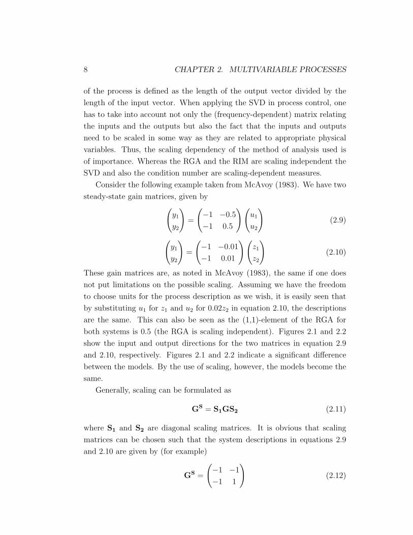
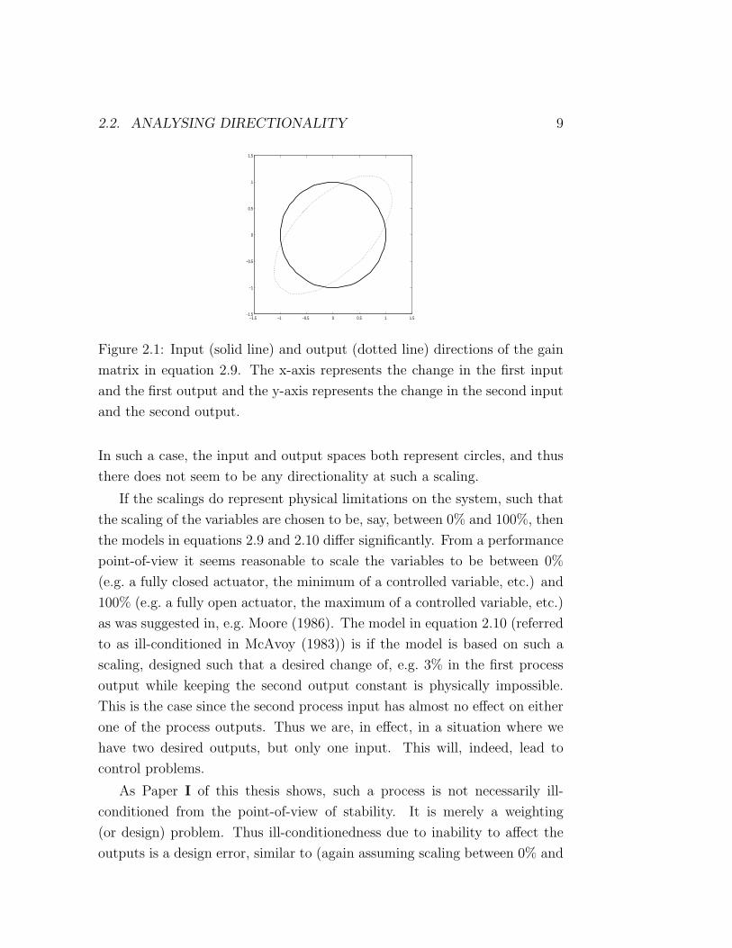
both systems is 0.5 (the RGA is scaling independent). Figures 2.1 and 2.2

show the input and output directions for the two matrices in equation 2.9

and 2.10, respectively. Figures 2.1 and 2.2 indicate a significant difference

between the models. By the use of scaling, however, the models become the

same.

Generally, scaling can be formulated as

GS = S1GS2 (2.11)

where S1 and S2 are diagonal scaling matrices. It is obvious that scaling

matrices can be chosen such that the system descriptions in equations 2.9

and 2.10 are given by (for example)

GS =

(−1 −1

−1 1

)(2.12)


−1.5 −1 −0.5 0 0.5 1 1.5−1.5

−1

−0.5

0

0.5

1

1.5

Figure 2.1: Input (solid line) and output (dotted line) directions of the gain

matrix in equation 2.9. The x-axis represents the change in the first input

and the first output and the y-axis represents the change in the second input

and the second output.

In such a case, the input and output spaces both represent circles, and thus

there does not seem to be any directionality at such a scaling.

If the scalings do represent physical limitations on the system, such that

the scaling of the variables are chosen to be, say, between 0% and 100%, then

the models in equations 2.9 and 2.10 differ significantly. From a performance

point-of-view it seems reasonable to scale the variables to be between 0%

(e.g. a fully closed actuator, the minimum of a controlled variable, etc.) and

100% (e.g. a fully open actuator, the maximum of a controlled variable, etc.)

as was suggested in, e.g. Moore (1986). The model in equation 2.10 (referred

to as ill-conditioned in McAvoy (1983)) is if the model is based on such a

scaling, designed such that a desired change of, e.g. 3% in the first process

output while keeping the second output constant is physically impossible.

This is the case since the second process input has almost no effect on either

one of the process outputs. Thus we are, in effect, in a situation where we

have two desired outputs, but only one input. This will, indeed, lead to

control problems.

As Paper I of this thesis shows, such a process is not necessarily ill-

conditioned from the point-of-view of stability. It is merely a weighting

(or design) problem. Thus ill-conditionedness due to inability to affect the

outputs is a design error, similar to (again assuming scaling between 0% and


−1.5 −1 −0.5 0 0.5 1 1.5−1.5

−1

−0.5

0

0.5

1

1.5





100%) the control of

(y1

y2

)=

(1 0

0 0.01

) (u1

u2

)(2.13)

This represents two independent control loops, each with one input and one

output. Obviously there is no interaction and thus this is not really a mul-

tivariable process, but still there is ”ill-conditionedness” as the condition

number is 100. Also, there will surely be control problems in the second

loop, as a 100% (full range) change in the manipulator results in a 1% per-

cent change of the defined range in the controlled output. Thus, this is not

a process where we actually can make sufficient changes in the manipulators

to drive the outputs over the entire range of interest. The same applies for

the process in equation 2.10.

All models discussed above are actually well-conditioned as long as we

have the freedom to choose the scaling. However, there is another kind of

ill-conditioned plants, which are ill-conditioned regardless of scaling. Such

cases are close to singular in the sense that although both inputs have a

strong impact on the outputs, the way either of these inputs affects both

the outputs is almost identical. Thus it will be difficult to separate them.


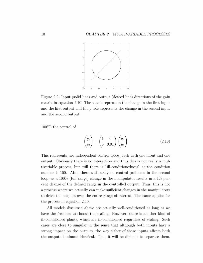
Assume a gain matrix according to(

y1

y2

)=

(−1 0.95

−0.95 1

)(u1

u2

)(2.14)

For such a matrix, the input and output directions represent a graph accord-

ing to figure 2.3. This matrix is optimally scaled, i.e. it cannot be rescaled in

−1.5 −1 −0.5 0 0.5 1 1.5−1.5

−1

−0.5

0

0.5

1

1.5





any way so that the output vector would be closer to a circle. The possible

effect of the scaling on the degree of directionality is not clear merely by

looking at the graphs. Thus, it is important to use the full range of measures

available.

Scaling is thus a key component in directionality analysis. One way to

keep the focus on control engineering and not design issues is to assume that

we have defined the operating ranges of our manipulators and our outputs

in such a way that one manipulator can drive one output anywhere within

the desired operating range, as long as the other loops are on manual, etc.

In such a case, the difficulties in the control which might rise are due to the

multivariable nature, and thus to the interaction and/or the directionality,

of the plant, not to the design issues.

An optimal scaling is the scaling that minimises the condition number.

Two optimally scaled matrices, with the same amount of interaction in the


sense that the magnitude of the Rijnsdorp interaction measure is the same,

are given by

K1 =

(1 k12

−k12 1

)(2.15)

K2 =

(1 k12

k12 1

)(2.16)

As k12 goes from 0 towards 1 for K1, the determinant goes from 1 to 2. This

is the well-conditioned case, which is the case for 2 × 2 systems, if the ma-

trix elements have an odd number of negative signs. The well-conditioned

case does not bring the matrix closer to singularity although the interaction

increases. This is also seen as the well-conditioned case has a mimimised

condition number = 1. For K2, which is the ill-conditioned case, the deter-

minant goes from 1 towards 0 as k12 goes from 0 towards 1, and thus the

matrix comes closer to singularity. This is the case for 2 × 2 systems if the

matrix elements have an even number of negative signs.

Again, as more thoroughly discussed in Paper I of this thesis and also in

Waller, Sagfors and Waller (1994a) and Waller, Sagfors and Waller (1994b),

scaling when analysing stability issues is irrelevant, and a scaling indepen-

dent measure should be used (e.g. RGA or the minimised condition number,

γmin). However, when it comes to analysing potential performance issues

(e.g. compare weights), scaling can be used to emphasise the differences in

the variables.

As seen, the scaling dependency can cause some confusion even for the lin-

ear case when analysing processes with potentially high directionality. Moore

(1986), Andersen and Kummel (1991) and Andersen and Kummel (1992) rec-

ommend a scaling dependent on the relative importance of variables or on

the physical limitations. Many authors, such as Lau, Alvarez and Jensen

(1985), Andersen, Laroche and Morari (1991) and Papastathopoulou and

Luyben (1991) seem to prefer physical scaling. Other papers, such as Gros-

didier, Morari and Holt (1985)and Skogestad and Morari (1987) seem to take

the view that the scaling that minimises the condition number is the correct

one. Often, the process model used is merely assumed to be properly scaled

(Brambilla and D’Elia, 1992; Freudenberg, 1989; Freudenberg, 1993). This is

2.3. CONTROLLING ILL-CONDITIONED PLANTS 13

further discussed in Paper I of this thesis, and in the references Waller et al.

(1994a) and Waller et al. (1994b).

2.3 Controlling ill-conditioned plants

As ill-conditioned plants are a subgroup of multivariable plants in general,

multivariable control in general is applied to controlling ill-conditioned plants.

In this thesis we briefly discuss two approaches to multivariable control. First,

we shall look at control structures including decoupling (see also Paper II of

this thesis and the references Waller and Waller (1991a), Waller and Waller

(1991b) and Waller and Waller (1992)).

In process control, the use of decoupling is well established (Luyben,

1970; Waller, 1974). Furthermore, it is well known (McAvoy, 1983) that

ill-conditioned processes are difficult to control by the use of decoupling.

According to McAvoy (1983), this is due to the increased sensitivity of the

ill-conditioned plant to disturbances.

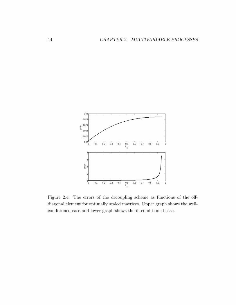
To illustrate the sensitivity of the decoupling approaches, we can look at

the matrices in equation 2.15 and 2.16. Assume the formulation that either

K1 or K2 represent the actual plant to be decoupled and that the matrix

used for calculating the decoupling is referred to as K1 and K2, respectively.

The decoupling matrix is thus (for example) D1 = (K1)−1 and D2 = (K2)

−1.

If K1 and K2 include errors as compared to K1 and K2 of no more than

+/-2% in each element, we can calculate the error of the decoupling strategy

for example as

Ei = max ||(I−DiKi)||2 (2.17)

The errors are visualised for the two matrices in figure 2.4 as functions of the

off-diagonal element k12.

Another approach to controlling ill-conditioned plants is a computation-

based approach, which is presented in the sequel and in Paper V of this

thesis.


0 0.1 0.2 0.3 0.4 0.5 0.6 0.7 0.8 0.9 10.02

0.022

0.024

0.026

0.028

0.03

k12

err

or

0 0.1 0.2 0.3 0.4 0.5 0.6 0.7 0.8 0.9 10

1

2

3

4

k12

err

or

Figure 2.4: The errors of the decoupling scheme as functions of the off-

diagonal element for optimally scaled matrices. Upper graph shows the well-

conditioned case and lower graph shows the ill-conditioned case.

Chapter 3

Nonlinearity

Analysing the multivariable nature of a plant, such as interaction and direc-

tionality, as done above, is not enough to assure a thorough understanding of

the plant studied and, thus, to achieve potential for good control. Many pro-

cesses of industrial importance, such as the distillation process, often show

both high directionality and interaction and also strong nonlinearity. Thus,

modelling techniques for nonlinear ill-conditioned plants are of importance.

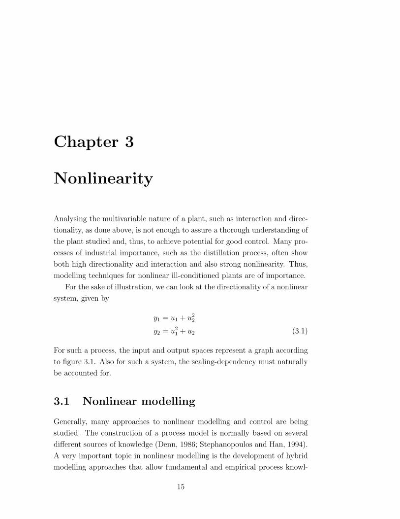
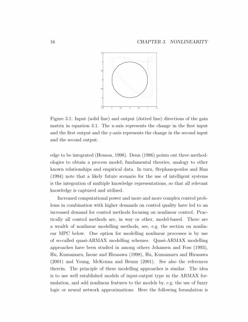
For the sake of illustration, we can look at the directionality of a nonlinear

system, given by

y1 = u1 + u22

y2 = u21 + u2 (3.1)

For such a process, the input and output spaces represent a graph according

to figure 3.1. Also for such a system, the scaling-dependency must naturally

be accounted for.

3.1 Nonlinear modelling

Generally, many approaches to nonlinear modelling and control are being

studied. The construction of a process model is normally based on several

different sources of knowledge (Denn, 1986; Stephanopoulos and Han, 1994).

A very important topic in nonlinear modelling is the development of hybrid

modelling approaches that allow fundamental and empirical process knowl-

15

16 CHAPTER 3. NONLINEARITY

−1.5 −1 −0.5 0 0.5 1 1.5−1.5

−1

−0.5

0

0.5

1

1.5





edge to be integrated (Henson, 1998). Denn (1986) points out three method-

ologies to obtain a process model; fundamental theories, analogy to other

known relationships and empirical data. In turn, Stephanopoulos and Han

(1994) note that a likely future scenario for the use of intelligent systems

is the integration of multiple knowledge representations, so that all relevant

knowledge is captured and utilised.

Increased computational power and more and more complex control prob-

lems in combination with higher demands on control quality have led to an

increased demand for control methods focusing on nonlinear control. Prac-

tically all control methods are, in way or other, model-based. There are

a wealth of nonlinear modelling methods, see, e.g. the section on nonlin-

ear MPC below. One option for modelling nonlinear processes is by use

of so-called quasi-ARMAX modelling schemes. Quasi-ARMAX modelling

approaches have been studied in among others Johansen and Foss (1993),

Hu, Kumamaru, Inoue and Hirasawa (1998), Hu, Kumamaru and Hirasawa

(2001) and Young, McKenna and Bruun (2001). See also the references

therein. The principle of these modelling approaches is similar. The idea

is to use well established models of input-output type in the ARMAX for-

mulation, and add nonlinear features to the models by, e.g. the use of fuzzy

logic or neural network approximations. Here the following formulation is

3.1. NONLINEAR MODELLING 17

considered as an example of a nonlinear quasi-ARMAX modelling approach.

For a more thorough presentation, please see Papers III and IV of this thesis

and the references therein.

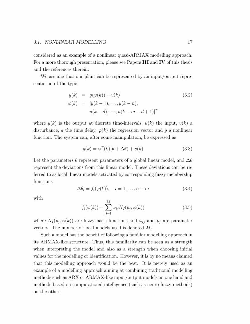
We assume that our plant can be represented by an input/output repre-

sentation of the type

y(k) = g(ϕ(k)) + v(k) (3.2)

ϕ(k) = [y(k − 1), . . . , y(k − n),

u(k − d), . . . , u(k −m− d + 1)]T

where y(k) is the output at discrete time-intervals, u(k) the input, v(k) a

disturbance, d the time delay, ϕ(k) the regression vector and g a nonlinear

function. The system can, after some manipulation, be expressed as

y(k) = ϕT (k)(θ + ∆θ) + v(k) (3.3)

Let the parameters θ represent parameters of a global linear model, and ∆θ

represent the deviations from this linear model. These deviations can be re-

ferred to as local, linear models activated by corresponding fuzzy membership

functions

∆θi = fi(ϕ(k)), i = 1, . . . , n + m (3.4)

with

fi(ϕ(k)) =M∑

j=1

ωijNf (pj, ϕ(k)) (3.5)

where Nf (pj, ϕ(k)) are fuzzy basis functions and ωij and pj are parameter

vectors. The number of local models used is denoted M .

Such a model has the benefit of following a familiar modelling approach in

its ARMAX-like structure. Thus, this familiarity can be seen as a strength

when interpreting the model and also as a strength when choosing initial

values for the modelling or identification. However, it is by no means claimed

that this modelling approach would be the best. It is merely used as an

example of a modelling approach aiming at combining traditional modelling

methods such as ARX or ARMAX-like input/output models on one hand and

methods based on computational intelligence (such as neuro-fuzzy methods)

on the other.


3.2 Nonlinear control and the NMPC formu-

lation

According to Takatsu et al. (1998), in a survey on industrially implemented

advanced control methodologies, and Qin and Badgwell (1998), model pre-

dictive control (in the sequel denoted MPC) and fuzzy control techniques are

increasingly employed especially in the refinery and petrochemical industries.

In this thesis the nonlinear model predictive control formulation is used as

an example of a successful method of implementing nonlinear control. MPC

is here used to describe a family of control methods, all having the same

characteristic features. These controllers are also referred to as receding or

moving horizon controllers.

The strong position MPC has reached in certain industrial fields is prob-

ably due to the straightforward design procedure, a clear open-loop optimi-

sation approach and the ease with which the method handles the process

model (Camacho and Bordons, 1999). In addition, a main motivation be-

hind the use of MPC is that MPC can easily incorporate constraints on the

variables already at the design stage of the controller. It is worth noting that

although many processes under MPC control are nonlinear by nature, the

vast majority of MPC applications are based on a linear model (referred to as

linear MPC). These linear models are commonly derived simply from step or

impulse identification experiments (Qin and Badgwell, 1998; Camacho and

Bordons, 1999).

The idea of the MPC formulation is to perform a (possibly time-consuming)

minimisation of a loss function with respect to a number of future control

moves (a control horizon) at every sampling instant. The loss function is

a function of these control moves and predicted process outputs. For the

prediction, in turn, a process model is used. The controller implements a

receding strategy so that at each instant the horizon is displaced towards

the future, which involves the application of the first control signal of the

sequence calculated at each step.

MPC can be described as an open-loop optimal control technique where

feedback is incorporated via the receding horizon formulation (Henson, 1998).

This open-loop optimality corresponds to a sub-optimal feedback control

3.2. NONLINEAR CONTROL AND THE NMPC FORMULATION 19

strategy (Yang and Polak, 1993). This fact is excellently illustrated in Rawl-

ings, Meadows and Muske (1994), where, for a certain control problem with

stochastic disturbances, the MPC only achieves 36% of the possible cost

reduction achievable by feedback control.

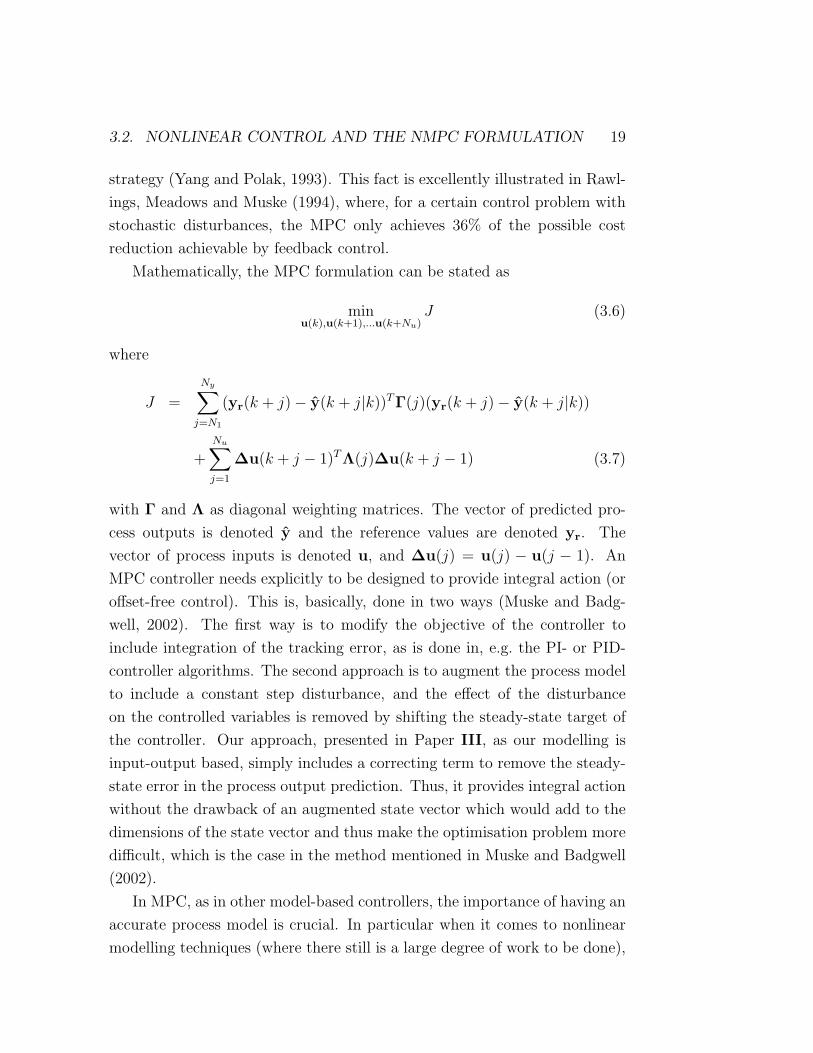
Mathematically, the MPC formulation can be stated as

minu(k),u(k+1),...u(k+Nu)

J (3.6)

where

J =

Ny∑j=N1

(yr(k + j)− y(k + j|k))TΓ(j)(yr(k + j)− y(k + j|k))

+Nu∑j=1

∆u(k + j − 1)TΛ(j)∆u(k + j − 1) (3.7)

with Γ and Λ as diagonal weighting matrices. The vector of predicted pro-

cess outputs is denoted y and the reference values are denoted yr. The

vector of process inputs is denoted u, and ∆u(j) = u(j) − u(j − 1). An

MPC controller needs explicitly to be designed to provide integral action (or

offset-free control). This is, basically, done in two ways (Muske and Badg-

well, 2002). The first way is to modify the objective of the controller to

include integration of the tracking error, as is done in, e.g. the PI- or PID-

controller algorithms. The second approach is to augment the process model

to include a constant step disturbance, and the effect of the disturbance

on the controlled variables is removed by shifting the steady-state target of

the controller. Our approach, presented in Paper III, as our modelling is

input-output based, simply includes a correcting term to remove the steady-

state error in the process output prediction. Thus, it provides integral action

without the drawback of an augmented state vector which would add to the

dimensions of the state vector and thus make the optimisation problem more

difficult, which is the case in the method mentioned in Muske and Badgwell

(2002).

In MPC, as in other model-based controllers, the importance of having an

accurate process model is crucial. In particular when it comes to nonlinear

modelling techniques (where there still is a large degree of work to be done),


the nonlinear model used for NMPC should be given extra attention. The

steps in a nonlinear identification problem are (as in linear identification)

listed by Henson (1998) as structure selection, input sequence design, noise

modelling, parameter estimation and model validation. Each of these poses

more challenging theoretical questions than their linear counterparts.

The types of discrete-time nonlinear models utilised for NMPC in the

recent literature include

• Hammerstein and Wiener models (for example in Fruzzetti, Palazoglu

and MacDonald (1997), Bloemen, Chu, van den Boom, Verdult, Verha-

gen and Backx (2001) and Pomerleau, Pomerleau, Hodouin and Poulin

(2003))

• Volterra models (Maner, Doyle, Ogunnaike and Pearson, 1996; Maner

and Doyle, 1997)

• Polynomial ARMAX (Banerjee and Arkun, 1998)

• Artificial neural networks (Arahal, Berenguel and Camacho, 1998; Ro-

hani, Haeri and Wood, 1999a; Rohani, Haeri and Wood, 1999b; Piche,

Sayyar-Rodsari, Johnson and Gerules, 2000)

• Fuzzy logic models (Sousa, Babuska and Verbruggen, 1997; Fisher,

Nelles and Isermann, 1998)

MPC is well covered in the literature, see, e.g. Camacho and Bordons

(1999) and Rawlings (2000). Excellent surveys and tutorials on NMPC can

be found in for example Rawlings et al. (1994) and Henson (1998). An

overview of industrial applications of advanced control methods in general

can be found in Takatsu et al. (1998) and of NMPC in particular in Qin and

Badgwell (1998). Texts focusing on the optimisations required for NMPC are,

for example, Mayne (1995), Biegler (1998) and Gopal and Biegler (1998). See

also Hussain (1999) for a survey of process control applications using MPC

with neural networks. A short introduction to some of the applications in

nonlinear MPC recently presented follows.

- Sousa et al. (1997) present NMPC based on a Takagi-Sugeno fuzzy model

used for the prediction. The controller proposed is a combination of a model

3.2. NONLINEAR CONTROL AND THE NMPC FORMULATION 21

predictive controller and an inverse based controller (IMC). If no constraints

are violated, an inverse based control algorithm is used. When constraints

are violated, the required optimisation used is a branch-and-bound algorithm.

Sousa et al. (1997) illustrate their controller by applying it to a laboratory

scale air-conditioning system.

- Fruzzetti et al. (1997) use simulation studies of a pH-process and a bi-

nary distillation column to illustrate their proposed controller. The model

used is a Hammerstein model with the motivation that many chemical pro-

cesses can be modelled as such, i.e. as a static nonlinearity followed by a

linear dynamical model. The optimisation algorithm used is an ellipsoidal

cutting-plane algorithm.

- Banerjee and Arkun (1998) present nonlinear MPC for control of plants

that operate in several distinct operating regions, and for the control during

the transition between these regions. The method used is to identify sev-

eral linear models and interpolate the nonlinear model between the linear

ones. The nonlinear model structure used is a polynomial ARX-model. The

resulting nonlinear MPC controller is applied to a CSTR example.

- Arahal et al. (1998) apply neural predictors to generalized predictive

control (one version of MPC) for nonlinear control. They apply their con-

troller to a solar power plant. The control scheme is implemented in such a

way that the response of the plant is divided into a free and a forced term

(Camacho and Bordons, 1999). A linear model is then used for the forced

part (thus making calculations of the optimal control sequence straightfor-

ward) and a nonlinear model for the free part (taking into account the effect

of perturbations).

- Rohani et al. (1999b) look at model predictive control and Rohani et al.

(1999a) discuss appropriate models (linear and nonlinear) for the purpose.

The process studied is (simulations of) a crystallisation process under NMPC

control with a model based on a feedforward neural network. The process is

multivariable with significant interaction.


Chapter 4

Approximating control

strategies

As the NMPC formulation above can be extremely time consuming, due to

the nonlinear optimisation problem to be solved at every sampling instant

(compare equation 3.6), there might be a need to relax the computational

burden. This is especially important for control problems with a short sam-

pling time. Different possibilities to perform such relaxation exist. These

include use of a linear model (and thus a linear MPC formulation) even for

control of nonlinear processes or use of short prediction and control horizons.

Another way to approach this problem is to use nonlinear function approx-

imators, designed to approximate, e.g. the behaviour of the nonlinear MPC

controller. Such approximations are discussed in Papers VI and VII of this

thesis, and in, e.g. Parisini and Zoppoli (1995), Gomez Ortega and Cama-

cho (1996), Parisini and Zoppoli (1998) and Cavagnari, Magni and Scattolini

(1999).

As one formulates the issue of approximating optimal or near-optimal

control actions, the problem can be formulated in at least two different ways.

On the one hand, given a certain state, an approximator can approximate

the designated control action. The controller then takes this action and

the procedure is repeated from the resulting state. We shall refer to this

as approximation of the control policy. On the other hand, it is possible to

approximate the smallest future cost taking a certain action in a certain state

23

24 CHAPTER 4. APPROXIMATING CONTROL STRATEGIES

will give rise to. If such an approximator is capable of approximating the

whole state-action space, then it is possible to choose the best action to take

from such an approximation of the value function, or cost-to-go function.

This will be referred to as an approximation of the value function.

4.1 Neurodynamic programming

The idea of approximating the value function corresponding to a state-action

set is similar to neurodynamic programming (Bertsekas and Tsitsiklis, 1996;

Haykin, 1999) and reinforcement learning (Sutton and Barto, 1998) and thus

also to Q-learning (Sutton and Barto, 1998; Hagen, 2001). The value function

can, in reinforcement learning terms, be said to represent the future sum of

expected reinforcements associated with a given state,

minu(k)

V (S(k),u(k)) (4.1)

The notation V (k) is used to denote the value function V (S(k),u(k)) in the

sequel, for the sake of simplicity. A common formulation of the value function

is to calculate V (k) as a quadratic loss function according to

V (k) =∞∑

j=k

(u(j)− u(j − 1))TΛ(u(j)− u(j − 1))

+∞∑

j=k+1

(ysp(j)− y(j))TΓ(ysp(j)− y(j)) (4.2)

The value (or loss) function thus represents a weighted sum of the loss in

future control moves and future errors between the reference values (i.e. the

set-points) and the actual process outputs. In practice, ∞ is replaced by a

sufficiently long horizon. The loss function can be replaced by an immediate

loss function and a future cost-to-go according to the dynamic programming

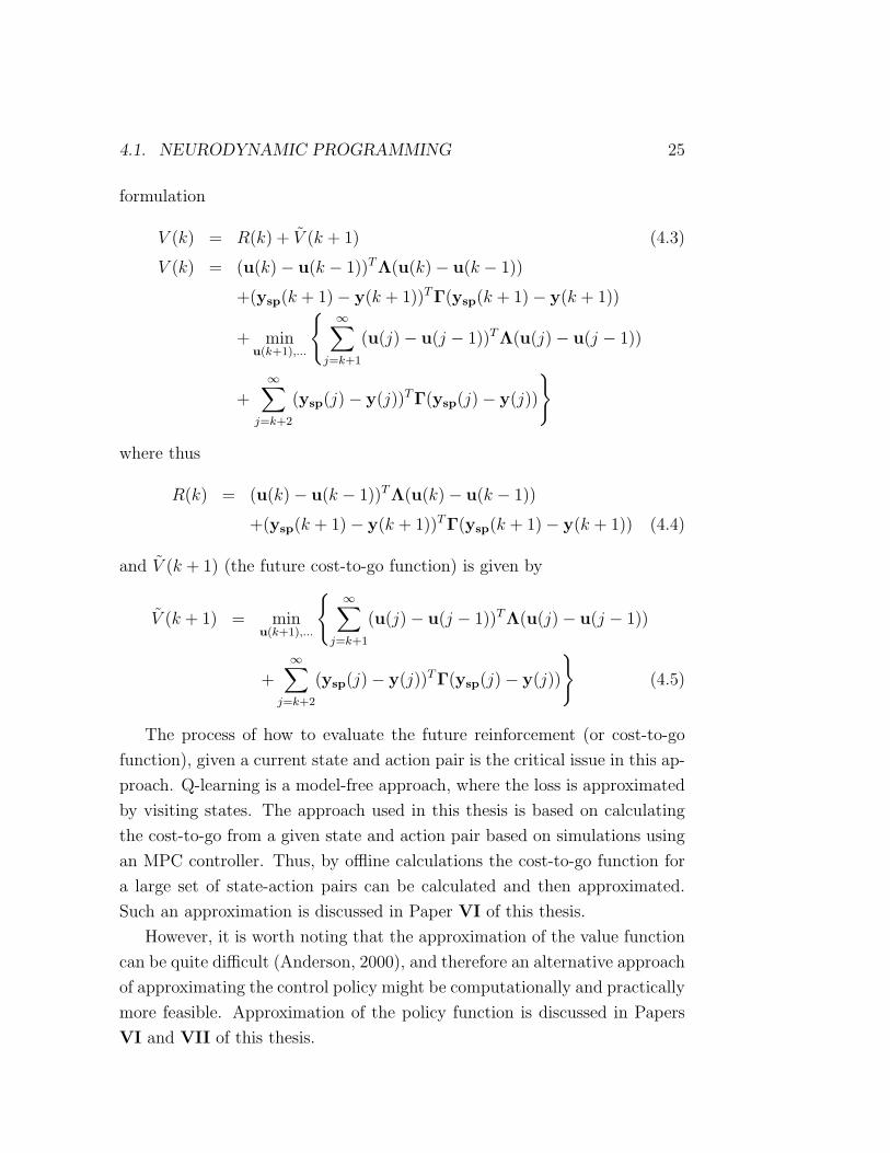
4.1. NEURODYNAMIC PROGRAMMING 25

formulation

V (k) = R(k) + V (k + 1) (4.3)

V (k) = (u(k)− u(k − 1))TΛ(u(k)− u(k − 1))

+(ysp(k + 1)− y(k + 1))TΓ(ysp(k + 1)− y(k + 1))

+ minu(k+1),...

{ ∞∑

j=k+1

(u(j)− u(j − 1))TΛ(u(j)− u(j − 1))

+∞∑

j=k+2

(ysp(j)− y(j))TΓ(ysp(j)− y(j))

}

where thus

R(k) = (u(k)− u(k − 1))TΛ(u(k)− u(k − 1))

+(ysp(k + 1)− y(k + 1))TΓ(ysp(k + 1)− y(k + 1)) (4.4)

and V (k + 1) (the future cost-to-go function) is given by

V (k + 1) = minu(k+1),...

{ ∞∑

j=k+1

(u(j)− u(j − 1))TΛ(u(j)− u(j − 1))

+∞∑

j=k+2

(ysp(j)− y(j))TΓ(ysp(j)− y(j))

}(4.5)

The process of how to evaluate the future reinforcement (or cost-to-go

function), given a current state and action pair is the critical issue in this ap-

proach. Q-learning is a model-free approach, where the loss is approximated

by visiting states. The approach used in this thesis is based on calculating

the cost-to-go from a given state and action pair based on simulations using

an MPC controller. Thus, by offline calculations the cost-to-go function for

a large set of state-action pairs can be calculated and then approximated.

Such an approximation is discussed in Paper VI of this thesis.

However, it is worth noting that the approximation of the value function

can be quite difficult (Anderson, 2000), and therefore an alternative approach

of approximating the control policy might be computationally and practically

more feasible. Approximation of the policy function is discussed in Papers

VI and VII of this thesis.

26 CHAPTER 4. APPROXIMATING CONTROL STRATEGIES

Chapter 5

Outline of the papers

5.1 Paper I

Defining Directionality: Use of Directionality Measures

with Respect to Scaling

In the first article of the thesis, the definitions of the concepts of directionality

and ill-conditionedness are studied and an investigation of the use of these

terms in the process control literature is carried out. The paper illustrates

that the commonly used definition of directionality is insufficient, due to the

wide range of different applications connected to directionality studied in the

field of process control. The paper points out that, due to this, the concept

of directionality is occasionally used in a somewhat confusing manner.

Directionality is closely related to the singular value decomposition, which

in turn is a method used in matrix algebra to measure, among other things,

how close a matrix is to being singular. One of the measures used in the

literature to measure directionality is the condition number, i.e. the largest

singular value divided by the smallest singular value.

In practical cases, however, the matrices studied actually represent pro-

cess models. These process model matrices are strongly influenced by the

units used to model the system. This fact is recognised by the singular value

decomposition (SVD) in the sense that the SVD is scaling dependent. Thus,

an analysis of directionality, or ill-conditionedness, must first treat the scal-

27

28 CHAPTER 5. OUTLINE OF THE PAPERS

ing question and choose a scaling in accordance with the analysis at hand.

If this is not done and scaling is performed based on, e.g. physical units,

it would imply that the control difficulties related to directionality would

change depending on whether it is, for instance, a British or a French engi-

neer that examines the process. Other measures also used in directionality

analysis such as the relative gain array or the minimised condition number

are scaling independent.

By examining the use of the concept of directionality, a refinement of

the definition of directionality is proposed so as to give a more meaningful

measure. The refinement divides the concept of directionality into two parts,

which are connected to stability and performance aspects, respectively. The

refinement of the definition clarifies the connection between control difficul-

ties and directionality and it also contributes to clarifying the scaling choice

when modelling a process with respect to directionality analysis.

5.2 Paper II

Decoupling Revisited

Approaches to controlling multivariable processes by the use of simple, intu-

itive means have commonly been popular in process control. Such approaches

include ”common-sense” methods, such as decoupling. Decoupling, in turn,

can be seen as a special implementation of a control structure. Decoupling

has been particularly well-used and successful in distillation control. Thus,

the field of distillation has seen several methods of designing decoupling con-

trollers, such as steady-state decoupling, ideal decoupling or simplified de-

coupling.

However, these common methods in distillation control have not gained

recognition in all fields of control. To illustrate this, an example from the

literature is picked for further study, where decoupling schemes originally

designed for distillation control are applied to control of a solid-fuel boiler.

A dynamic decoupling approach performs well as compared to the original

static decoupler proposed in the literature, as expected.

In addition, a reformulation of the design procedure when designing dy-

5.3. PAPER III 29

namic decouplers is presented. This reformulation makes it easier always to

find a realisable dynamic decoupler for the process at hand by adding the

necessary dynamics to the primary control loops.

5.3 Paper III

Nonlinear Model Predictive Control Utilizing a Neuro-

Fuzzy Predictor

Nonlinearity is another of the main challenges facing the field of process

control. Thus, in the third paper, the focus is temporarily shifted away from

ill-conditioned plants, and instead concentrates on the nonlinearity often

associated with process control problems.

The third paper thus investigates nonlinear modelling techniques for use

with the MPC controller in a process control environment. A modelling

technique of quasi-ARMAX type which recently has been presented in the

literature is discussed as regards process control applications and formulated

to be used in the MPC framework.

In association with the nonlinear modelling technique, the (nonlinear)

MPC controller formulation is investigated. This is done by looking at simple

examples of control problems emphasising the challenge of processes with a

dynamic behaviour that changes with the operating region, as is often the

case in process control.

The nonlinear modelling scheme studied here has the benefit of being

similar to the commonly used input/output models of ARMAX-type. Thus,

it is well motivated for a straightforward controller approach such as the MPC

formulation and it retains the intuitive appeal of the MPC formulation.

5.4 Paper IV

A Neuro-Fuzzy Model Predictive Controller Applied to

a pH-neutralization Process

The fourth paper in the thesis continues where the third paper left off.

The paper investigates how the quasi-ARMAX modelling scheme works for


modelling a highly nonlinear pH-neutralization process. The nonlinearities of

the pH-process strongly depend on the operating region, and thus the quasi-

ARMAX model, consisting of a global model and of local models active in

different regions, is well suited to model such nonlinearities. This pH-process

has been used in several case-studies as an illustration of means to control

nonlinear plants. Please see the references in the paper.

The pH-process is then controlled to handle both set-point changes and

unmodelled disturbances by the use of the nonlinear model predictive control

formulation. Integral action is incorporated in the controller by correcting

the predicted output based on measurements of the last available output.

The controller works well as compared to other controllers for this process,

which have been studied in the literature.

5.5 Paper V

Multivariable Nonlinear MPC of an Ill-conditioned Dis-

tillation Column

The fifth paper in this thesis consists of an investigation of control of a

nonlinear and ill-conditioned distillation column. This paper thus works as a

conclusion of the part concerning quasi-ARMAX nonlinear model predictive

control.

First, the plant is investigated and the nonlinear ill-conditionedness of the

distillation column is characterised. The quasi-ARMAX model is reformu-

lated so as to model multivariable systems. The nonlinear MPC formulation,

including the integral action, is then used as a controller for control of two

compositions at the distillation column. Successful control of the nonlinear

ill-conditioned process both in the face of set-point changes and for eliminat-

ing the effect of unmodelled disturbances is illustrated.

5.6. PAPER VI 31

5.6 Paper VI

Value Function and Policy Approximation for Nonlinear

Control of a pH-neutralization Process

One of the main disadvantages of the MPC formulation is that it is often

computationally demanding. Thus, different approaches to relieve this com-

putational burden are of interest.

The formulation of control problems as optimisation problems of dynamic

programming-type has received a large interest in fields such as reinforcement

learning and neurodynamic programming. In such a formulation, the optimal

cost-to-go function is divided into an immediate cost and a future cost-to-go,

given a certain state. Thus, by estimating this future cost-to-go function by

some kind of function approximator, one can formulate the control problem

as a value function approximation.

In the sixth paper in this thesis, a value function approximating scheme

is investigated, first on a simple linear process and then on the pH-process

used in Paper IV. The future cost-to-go function is then approximated by

the use of a feedforward neural network. For training of the neural network

used for the function approximation, the future control moves are calculated

by use of a nonlinear MPC formulation.

As the approximation of the value function demands much data, an al-

ternative strategy is a formulation where the optimal control policy is ap-

proximated instead. In the paper this is also shown to work well for control

of the pH-process.

5.7 Paper VII

Neural Network Approximation of a Nonlinear Model

Predictive Controller Applied to a pH Neutralization

Process

The concept of approximating the optimal control policy introduced in Paper

VI is taken further in this paper.


In this paper, the pH-process is modelled by a set of linearised models

obtained by velocity-based linearisation. The velocity-based linearisation

uses the latest measurement of the pH-value as the scheduling variable. In

theory, the nonlinear plant could be described exactly by a set of linearised

models, although in practice errors are unavoidable.

A neural network function approximator is then used to approximate the

velocity-based linearised model predictive control strategy. The network used

is a feedforward neural network. Furthermore, the controller includes integral

action.

The accuracy of the neural network controller approximation which is

required to ensure stability and performance is shown to be related to the

fragility of the original model predictive controller, and it can be charac-

terised in terms of an l2-induced norm defined for the closed-loop system.

Chapter 6

Conclusions

This thesis addresses some relevant problems in the field of process control.

First, an analysis of the multivariable nature of process models is made.

The terminology, such as directionality, interaction and scaling, is clarified.

Inconsistencies in the common use of this terminology are pointed out. Fur-

ther, a consistent use of this terminology makes it possible to relate it to

robustness and performance aspects, respectively.

This indicates how an improved understanding of the concepts of inter-

action, directionality and scaling can improve the analysis and thus also the

quality of control results in multivariable process control.

Second, ”conventional intelligence” in the form of control structures is

applied as a means to deal with the problem of controlling multivariable,

possibly nonlinear, plants. Decoupling, which is a control structure com-

monly used in process control, is discussed and studied as an example of

how basic process understanding or, if one wishes, basic engineering wisdom,

can be used to solve seemingly difficult control problems in an intuitively

appealing and efficient manner.

The interaction between different control loops is, as mentioned, consid-

ered to be one of the main challenges in process control. Another significant

challenge in process control is handling the nonlinear features of the process

under control. As a means to tackle this challenge this thesis investigates

how an input/output based nonlinear modelling technique manages to cap-

ture the nonlinearities.

33

34 CHAPTER 6. CONCLUSIONS

Also, as computational capabilities increase, the emphasis in controller

implementation can shift towards more computation-demanding applications.

As such, this thesis has studied the model predictive control formulation for

use for control of some relevant processes. In particular, the model predictive

control formulation in conjunction with a quasi-ARMAX modelling technique

is studied. These studies are performed on case studies representing impor-

tant process control problems. A highly nonlinear pH-neutralization process

in a single-input single-output formulation is studied. Also, a binary dis-

tillation column is studied as it is highly challenging in the sense that it

exhibits both significant nonlinearity and ill-conditionedness. The technique

discussed here shows good results on both processes, as compared to other

results presented in the literature.

Furthermore, as the nonlinear MPC formulation might lead to extremely

time-consuming computations, techniques for approximating the behaviour

of the MPC controller by means of both value function and policy approx-

imating methods are studied. These approximation techniques manage to

reduce the computational burden significantly, without a significant reduc-

tion in control quality.

Although the potential of computation-intensive control methods, such

as computational intelligence and online optimisations, is large and posi-

tive results have been presented (Takatsu et al., 1998; Hussain, 1999), there

have been sometimes constructive but often destructive discussions concern-

ing traditional control versus (mainly) fuzzy control (Astrom and McAvoy,

1992; Kosko, 1993; Abramovitch, 1994; Bezdek, 1994; Zadeh, 1994; Zadeh,

1996; Abramovitch and Bushnell, 1999; Abramovitch, 1999; Ho, 1999). These

discussions could be seen as an indicative reference frame to the mentality

within the field of process control. As we see it, one of the main chal-

lenges in process control is the ability to combine the established methods,

including ad hoc methods, rule-of-thumb and engineering wisdom with the

computation-based cognitive methods based on computational intelligence

and computational power, such as fuzzy logic, neural networks and MPC

calculations. The potential gain of a more constructive cooperation is enor-

mous.

This thesis has tried to discuss two of the large challenges in process con-

35

trol, namely directionality and nonlinearity, from two different approaches.

First directionality is studied from the conventional wisdom approach, and

second, nonlinearity is studied from a computational approach. Furthermore,

on an introductory level this thesis discusses the meeting place of these two

approaches with the control of a nonlinear, ill-conditioned distillation column.

Here, the challenge does not lie in one of the two discussed problems, but

in both. Also, controllers able to combine the appeal of conventional meth-

ods, such as input/output modelling, with methods based on computational

intelligence, such as neuro-fuzzy modelling, in an environment allowing for

computation-intensive methods have been discussed. These controllers aim

at pointing toward the benefit of combining methods from different disci-

plines, in order to perform truly intelligent control in the future.

36 CHAPTER 6. CONCLUSIONS

Bibliography

Abramovitch, D. (1994). Some crisp thoughts on fuzzy logic, Proceedings of

the American Control Conference, Baltimore, Maryland, USA.

Abramovitch, D. Y. (1999). Fuzzy control as a disruptive technology, IEEE

Control Systems 19(3): 100–102.

Abramovitch, D. Y. and Bushnell, L. G. (1999). Report on the fuzzy versus

conventional control debate, IEEE Control Systems 19(3): 88–91.

Andersen, H. W. and Kummel, M. (1991). Identifying gain directionality of

multivariable processes, Proceedings of the ECC, pp. 1968–1973.

Andersen, H. W. and Kummel, M. (1992). Evaluating estimation of gain

directionality, part 1 and 2, J. Proc. Cont. 2: 59–66, 67–86.

Andersen, H. W., Laroche, L. and Morari, M. (1991). Dynamics of homoge-

neous azeotropic distillation columns, Ind. Eng. Chem. Res. 30: 1846–

1855.

Anderson, C. W. (2000). Approximating a policy can be easier than ap-

proximating a value function, Technical Report CS-00-101, Computer

Science, Colorado State University, Fort Collins, CO 80523-1873.

Arahal, M. R., Berenguel, M. and Camacho, E. F. (1998). Neural identifica-

tion applied to predictive control of a solar plant, Control Eng. Practice

6: 333–344.

Astrom, K. J. and Hagglund, T. (1995). PID Controllers: Theory, Design

and Tuning, ISA.

37

38 BIBLIOGRAPHY

Astrom, K. J. and McAvoy, T. J. (1992). Intelligent control, J. Proc. Cont.

2(3): 115–127.

Balchen, J. G. (1999). How have we arrived at the present state of knowledge

in process control? Is there a lesson to be learned?, J. Proc. Cont.

9: 101–108.

Balchen, J. G. and Mumme, K. I. (1988). Process Control: Structures and

Applications, Van Nostrand Reinhold.

Banerjee, A. and Arkun, Y. (1998). Model predictive control of plant tran-

sitions using a new identification technique for interpolating nonlinear

models, J. Proc. Cont. 8(5-6).

Bertsekas, D. P. and Tsitsiklis, J. N. (1996). Neuro-Dynamic Programming,

Athena Scientific.

Bezdek, J. (1994). Fuzziness vs. probability - again (! ?), IEEE Transactions

on Fuzzy Systems 2(1): 1–3.

Biegler, L. T. (1998). Advances in non-linear programming concepts for

process control, J. Proc. Cont. 8(5-6): 301–311.

Bloemen, H. H. J., Chu, C. T., van den Boom, T. J. J., Verdult, V., Ver-

hagen, M. and Backx, T. C. (2001). Wiener model identification and

predictive control for dual composition control of a distillation column,

J. Proc. Cont. 11: 601–620.

Brambilla, A. and D’Elia, L. (1992). Multivariable controller for distilla-

tion columns in the presence of strong directionality and model errors,

Ind. Eng. Chem. Res. 31: 536–543.

Bristol, E. H. (1966). On a new measure of interactions for multivariable

process control, IEEE Transactions on Automatic Control AC-11: 133–

134.

Camacho, E. F. and Bordons, C. (1999). Model Predictive Control, Springer

Verlag.

BIBLIOGRAPHY 39

Cavagnari, L., Magni, L. and Scattolini, R. (1999). Neural network imple-

mentation of nonlinear receding-horizon control, Neural Computing &

Applications 8: 86–92.

Chidambaram, M. and See, R. P. (2002). A simple method of tuning PID con-

trollers for integrator/dead-time processes, Comp. Chem. Eng. 27: 211–

215.

Denn, M. (1986). Process Modeling, Longman Scientific & Technical.

Fisher, M., Nelles, O. and Isermann, R. (1998). Adaptive predictive control of

a heat exchanger based on a fuzzy model, Control Eng. Practice 6: 259–

269.

Freudenberg, J. S. (1989). Analysis and design for ill-conditioned plants.

Part 2. Directionally uniform weightings and an example, Int. J. Control

49: 873–903.

Freudenberg, J. S. (1993). Algebraic versus analytic limitations imposed by

ill-conditioned plants, IEEE Trans. Autom. Control 38: 625–629.

Fruzzetti, K. P., Palazoglu, A. and MacDonald, K. A. (1997). Non-linear

model predictive control using Hammerstein models, J. Proc. Cont.

7(1): 31–41.

Golub, G. H. and Van Loan, C. F. (1996). Matrix Computations, 3rd edn,

The Johns Hopkins University Press.

Gomez Ortega, J. and Camacho, E. F. (1996). Mobile robot navigation in a

partially structured static environment, using neural predictive control,

Control Eng. Practice 4: 1669–1679.

Gopal, V. and Biegler, L. (1998). Large scale inequality constrained optimi-

sation and control, IEEE Control Systems 18(6): 59–68.

Grosdidier, P., Morari, M. and Holt, B. R. (1985). Closed-loop properties

from steady-state gain information, Ind. Eng. Chem. Fund. 24: 221–235.

40 BIBLIOGRAPHY

Hagen, S. H. (2001). Continuous State Space Q-Learning for Control of

Nonlinear Systems, PhD thesis, Universiteit van Amsterdam, Faculteit

der Natuurwetenschappen, Wiskunde en Informatica.

Haykin, S. (1999). Neural Networks. A Comprehensive Foundation, 2nd edn,

Prentice Hall.

Henson, M. A. (1998). Non-linear model predictive control: Current status

and future directions, Comp. Chem. Eng. 23: 187–202.

Ho, Y.-C. (1999). The no free lunch theorem and the human-machine inter-

face, IEEE Control Systems 19(3): 8–10.

Hu, J., Kumamaru, K. and Hirasawa, K. (2001). A quasi-ARMAX approach

to modelling of non-linear systems, Int. J. Control 74(18): 1754–1766.

Hu, J., Kumamaru, K., Inoue, K. and Hirasawa, K. (1998). A hybrid

quasi-ARMAX modeling scheme for identification of nonlinear systems,

Trans. SICE 34: 977–986.

Hussain, M. A. (1999). Review of the application of neural networks in chem-

ical process control - simulation and online implementation, Artificial

Intelligence in Engineering 13: 55–68.

Johansen, T. A. and Foss, B. A. (1993). Constructing NARMAX models

using ARMAX models, Int. J. Control 58(5): 1125–1153.

Kelly, K. (1994). Out of Control. The New Biology of Machines, Social

Systems, and the Economic World, Perseus Books.

Kosko, B. (1993). Fuzzy Thinking: The New Science of Fuzzy Logic, Hyper-

ion, New York.

Lau, H., Alvarez, J. and Jensen, K. F. (1985). Synthesis of control struc-

tures by singular value analysis: Dynamic measures of sensitivity and

interaction, AIChE J. 31: 427–439.

Luyben, W. L. (1970). Distillation decoupling, AIChE J. 16: 198.

BIBLIOGRAPHY 41

Luyben, W. L. (1992). Practical Distillation Control, Van Nostrand Reinhold.

Maner, B. R. and Doyle, F. J. I. (1997). Polymerization reactor control using

autoregressive-plus Volterra-based MPC, AIChE J. 43(7): 1763–1784.

Maner, B. R., Doyle, F. J. I., Ogunnaike, B. A. and Pearson, R. K.

(1996). Nonlinear model predictive control of a simulated multivariable

polymerization reactor using second-order Volterra models, Automatica

32(9): 1285–1301.

Mayne, D. Q. (1995). Optimisation in model based control, Proceedings of

IFAC Symposium DYCORD+’95, Helsingør, Denmark.

McAvoy, T. (1983). Interaction Analysis, ISA.

Moore, C. (1986). Application of SVD to the design, analysis and control of

industrial processes, Proceedings of the ACC, Seattle, WA, pp. 643–650.

Muske, K. R. and Badgwell, T. A. (2002). Disturbance modeling for offset-

free linear model predictive control, J. Proc. Cont. 12: 617–632.

Papastathopoulou, H. S. and Luyben, W. L. (1991). Control of a binary

sidestream distillation column, Ind. Eng. Chem. Res. 30: 705–713.

Parisini, T. and Zoppoli, R. (1995). A receding-horizon regulator for nonlin-

ear systems and a neural approximation, Automatica 31: 1443–1451.

Parisini, T. and Zoppoli, R. (1998). Neural approximations for infinite-

horizon optimal control of nonlinear stochastic systems, IEEE Trans. on

Neural Networks 9(6): 1388–1408.

Piche, S., Sayyar-Rodsari, B., Johnson, D. and Gerules, M. (2000). Nonlinear

model predictive control using neural networks, IEEE Control Systems

20(3): 53–62.

Pomerleau, D., Pomerleau, A., Hodouin, D. and Poulin, E. (2003). A

procedure for the design and evaluation of decentralised and model-

based predictive multivariable controllers for a pellet cooling process,

Comp. Chem. Eng. 27: 217–233.

42 BIBLIOGRAPHY

Qin, S. J. and Badgwell, T. A. (1998). An overview of non-linear model pre-

dictive control applications, Proceedings Workshop on NMPC, Ascona,

Switzerland.

Rauch, H. E. (1998). A control engineers use of artificial intelligence, Control

Eng. Practice 6: 249–258.

Rawlings, J. B. (2000). Tutorial overview of model predictive control, IEEE

Control Systems 20(3): 38–52.

Rawlings, J. B., Meadows, E. S. and Muske, K. R. (1994). Non-linear model

predictive control: A tutorial and a survey, Preprints IFAC Symposium

ADCHEM ’94, Kyoto Research Park, Kyoto, Japan.

Rijnsdorp, J. E. (1965). Interaction in two-variable control systems for dis-

tillation columns - 1. Theory, Automatica 3: 15–28.

Rohani, S., Haeri, M. and Wood, H. C. (1999a). Modeling and control of a

continuous crystallization process. Part 1. Linear and non-linear mod-

eling, Comp. Chem. Eng. 23: 263–277.

Rohani, S., Haeri, M. and Wood, H. C. (1999b). Modeling and control of

a continuous crystallization process. Part 2. Model predictive control,

Comp. Chem. Eng. 23: 279–286.

Seborg, D. E., Edgar, T. F. and Mellichamp, D. A. (1989). Process Dynamics

and Control, Wiley.

Shinskey, F. G. (1984). Distillation Control For Productivity and Energy

Conservation, 2nd edn, McGraw-Hill.

Skogestad, S. and Morari, M. (1987). Implications of large RGA elements on

control performance, Ind. Eng. Chem. Res. 26: 2323–2330.

Skogestad, S. and Postlethwaite, I. (1996). Multivariable Feedback Control,

Wiley.

Sousa, J. M., Babuska, R. and Verbruggen, H. B. (1997). Fuzzy predictive

control applied to an air-conditioning system, Control Eng. Practice

5(10): 1395–1406.

BIBLIOGRAPHY 43

Stephanopoulos, G. and Han, C. (1994). Intelligent systems in process engi-

neering: A review, Proceedings of the PSE ’94, Kyongju, Korea.

Sutton, R. S. and Barto, A. G. (1998). Reinforcement Learning. An Intro-

duction, The MIT Press.

Takatsu, H., Itoh, T. and Araki, M. (1998). Future needs for the control

theory in industries - report and topics of the control technology survey

in japanese industry, J. Proc. Cont. 8(5-6): 369–374.

Waller, J. B., Sagfors, M. F. and Waller, K. V. (1994a). Ill-conditionedness

and process directionality - the use of condition numbers in process con-

trol, Preprints IFAC Symposium ADCHEM ’94, Kyoto Research Park,

Kyoto, Japan.

Waller, J. B., Sagfors, M. F. and Waller, K. V. (1994b). The robustness of

ill-conditioned plants, Proceedings of the PSE ’94, Kyongju, Korea.

Waller, J. B. and Waller, K. V. (1991a). Parametrization of a disturbance

rejecting and decoupling control structure, Technical Report 91-13, Pro-

cess Control Laboratory, Department of Chemical Engineering, Abo

Akademi University, 20500 Abo, Finland.

Waller, J. B. and Waller, K. V. (1991b). Robustness and dynamic design of

disturbance rejecting and decoupling control structures, Technical Re-

port 91-15, Process Control Laboratory, Department of Chemical Engi-

neering, Abo Akademi University, 20500 Abo, Finland.

Waller, J. B. and Waller, K. V. (1992). Relating the DRD structure to

conventional model based controllers, Proceedings of DYCORD+ ’92,

Maryland, USA.

Waller, K. V. (1974). Decoupling in distillation, AIChE J. 20: 592.

Yang, T. H. and Polak, E. (1993). Moving horizon control of non-linear

systems with input saturation, disturbances and plant uncertainty,

Int. J. Control 58(4): 875–903.

44 BIBLIOGRAPHY

Young, P. C., McKenna, P. and Bruun, J. (2001). Identification of non-

linear stochastic systems by state dependent parameter estimation,

Int. J. Control 74(18): 1837–1857.

Zadeh, L. A. (1994). Fuzzy logic, neural networks, and soft computing,

Communications of the ACM 37(3): 77–84.

Zadeh, L. A. (1996). Fuzzy logic = computing with words, IEEE Trans. on

Fuzzy Systems 4(2): 103–111.

Ziegler, J. G. and Nichols, N. B. (1942). Optimum settings for automatic

controllers, Trans. ASME 64: 759–765.

Date post:	02-Aug-2018
Category:	Documents
Upload:	leduong
View:	213 times
Download:	0 times

Directionality and Nonlinearity - Challenges in Process...

Documents