165


In the IOCCG Report Series:
1. Minimum Requirements for an Operational Ocean-Colour Sensor for the Open Ocean
(1998)
2. Status and Plans for Satellite Ocean-Colour Missions: Considerations for Complementary
Missions (1999)
3. Remote Sensing of Ocean Colour in Coastal, and Other Optically-Complex, Waters (2000)
4. Guide to the Creation and Use of Ocean-Colour, Level-3, Binned Data Products (2004)
5. Remote Sensing of Inherent Optical Properties: Fundamentals, Tests of Algorithms, and
Applications (2006)
6. Ocean-Colour Data Merging (2007)
7. Why Ocean Colour? The Societal Benefits of Ocean-Colour Technology (2008)
8. Remote Sensing in Fisheries and Aquaculture (2009)
9. Partition of the Ocean into Ecological Provinces: Role of Ocean-Colour Radiometry (2009)
10. Atmospheric Correction for Remotely-Sensed Ocean-Colour Products (2010)
11. Bio-Optical Sensors on Argo Floats (2011)
12. Ocean-Colour Observations from a Geostationary Orbit (2012)
13. Mission Requirements for Future Ocean-Colour Sensors (2012)
14. In-flight Calibration of Satellite Ocean-Colour Sensors (2013)
15. Phytoplankton Functional Types from Space (2014)
16. Ocean Colour Remote Sensing in Polar Seas (2015)
17. Earth Observations in Support of Global Water Quality Monitoring (2018)
18. Uncertainties in Ocean Colour Remote Sensing (2019)
19. Synergy between Ocean Colour and Biogeochemical/Ecosystem Models (2020)
20. Observation of Harmful Algal Blooms with Ocean Colour Radiometry (this volume)
Disclaimer: The views expressed in this report are those of the authors and do not necessarily
reflect the views or policies of government agencies, or the IOCCG. Mention of trade names or
commercial products does not constitute endorsement or recommendation.
The printing of this report was sponsored and carried out by the State Key Laboratory of
Satellite Ocean Environment Dynamics, Second Institute of Oceanography, Ministry of Natural
Resources, China, which is gratefully acknowledged.

Reports and Monographs of the InternationalOcean Colour Coordinating Group
An Affiliated Program of the Scientific Committee on Oceanic Research (SCOR)
An Associated Member of the Committee on Earth Observation Satellites (CEOS)
IOCCG Report Number 20, 2021
Observation of Harmful Algal Blooms with Ocean ColourRadiometry
Edited by:
Stewart Bernard, Raphael Kudela, Lisl Robertson Lain and Grant Pitcher
Report of an IOCCG and GEOHAB/GlobalHAB working group chaired by Stewart Bernard and
based on contributions from (in alphabetical order):
Stewart Bernard South African National Space Agency, South Africa
Mariano Bresciani CNR-IREA, Italy
Jennifer Cannizzaro University of South Florida, USA
Hongtao Duan Nanjing Institute of Geography and Limnology, China
Claudia Giardino CNR-IREA, Italy
Patricia M. Glibert University of Maryland, USA
Chuanmin Hu University of South Florida, USA
Raphael M. Kudela University of Southern California, USA
Tiit Kutser University of Tartu, Estonia
Lisl Robertson Lain University of Cape Town, South Africa
Ronghua Ma Nanjing Institute of Geography and Limnology, China
Erica Matta CNR IREA, Italy
Mark W. Matthews CyanoLakes (Pty) Ltd, South Africa
Constant Mazeran SOLVO, France
Frank E. Muller-Karger University of South Florida, USA
Grant C. Pitcher Department of Environment, Forestry and Fisheries, South Africa
Suzanne Roy Université du Québec à Rimouski, Canada
Blake Schaeffer U.S. Environmental Protection Agency, USA
Stefan G. H. Simis Plymouth Marine Laboratory, UK
Marié E. Smith NRE Earth Observation, CSIR, South Africa
Inia M. Soto Universities Space Research Association, NASA GSFC, USA
Erin Urquhart Science Systems and Applications Inc., NASA GSFC, USA
Jennifer Wolny Maryland Department of Natural Resources, USA
Series Editor: Venetia Stuart

Correct citation for this publication:
IOCCG (2021). Observation of Harmful Algal Blooms with Ocean Colour Radiometry. Bernard, S., Kudela,
R., Robertson Lain, L. and Pitcher, G.C. (eds.), IOCCG Report Series, No. 20, International Ocean Colour
Coordinating Group, Dartmouth, Canada. http://dx.doi.org/10.25607/OBP-1042
This working group was sponsored jointly by the International Ocean Colour Coordinating Group
(IOCCG) as well as the GEOHAB Programme (now GlobalHAB) of the Scientific Committee on Oceanic
Research (SCOR) and the Intergovernmental Oceanographic Commission (IOC) of UNESCO. The IOCCG
is an international group of experts promoting the application of remotely-sensed ocean-colour and
inland water radiometric data across all aquatic environments, acting as a liaison and communication
channel between users, managers and agencies in the ocean colour arena.
The IOCCG is sponsored by the Centre National d’Etudes Spatiales (CNES, France), Canadian Space
Agency (CSA, Canada), Commonwealth Scientific and Industrial Research Organisation (CSIRO, Aus-
tralia), Department of Fisheries and Oceans (Bedford Institute of Oceanography, Canada), European
Commission/Copernicus Programme, European Organisation for the Exploitation of Meteorological
Satellites (EUMETSAT), European Space Agency (ESA), Indian Space Research Organisation (ISRO), Japan
Aerospace Exploration Agency (JAXA), Joint Research Centre (JRC, EC), Korea Institute of Ocean Science
and Technology (KIOST), National Aeronautics and Space Administration (NASA, USA), National Oceanic
and Atmospheric Administration (NOAA, USA), Scientific Committee on Oceanic Research (SCOR), and
the State Key Laboratory of Satellite Ocean Environment Dynamics (Second Institute of Oceanography,
Ministry of Natural Resources, China)
http: //www.ioccg.org
Published by the International Ocean Colour Coordinating Group,
P.O. Box 1006, Dartmouth, Nova Scotia, B2Y 4A2, Canada.
ISSN: 1098-6030
ISBN: 978-1-896246-66-6
©IOCCG 2021
Printed by the State Key Laboratory of Satellite Ocean Environment Dynamics, Second Institute of
Oceanography, Ministry of Natural Resources, China.

Contents
1 Introduction 9
1.1 HABs: Definition and Characterisation . . . . . . . . . . . . . . . . . . . . . . . . . . . 9
1.2 HAB Incidence and Impact . . . . . . . . . . . . . . . . . . . . . . . . . . . . . . . . . . . 10
1.3 Role of Ocean Colour Radiometry in HAB Studies . . . . . . . . . . . . . . . . . . . . 11
2 Harmful Algal Blooms, Changing Ecosystem Dynamics and Related Conceptual Models 13
2.1 Introduction to Harmful Algal Blooms and their Effects . . . . . . . . . . . . . . . . . 13
2.2 HABs and Global Change . . . . . . . . . . . . . . . . . . . . . . . . . . . . . . . . . . . . 15
2.2.1 Relationships with eutrophication . . . . . . . . . . . . . . . . . . . . . . . . . . 15
2.2.2 Relationships with changing climate . . . . . . . . . . . . . . . . . . . . . . . . 17
2.3 Trophic Interactions: HABs as Prey and as Predators . . . . . . . . . . . . . . . . . . 18
2.4 Conceptual Models of the Influence of Nutrients and the Physical Environment on
Species Selection . . . . . . . . . . . . . . . . . . . . . . . . . . . . . . . . . . . . . . . . . 19
2.5 The Global Ecology and Oceanography of Harmful Algal Blooms (GEOHAB) Pro-
gramme . . . . . . . . . . . . . . . . . . . . . . . . . . . . . . . . . . . . . . . . . . . . . . 23
3 Ocean Colour and Detecting Phytoplankton Biomass and Community Dynamics 25
3.1 HAB Observation by Satellite . . . . . . . . . . . . . . . . . . . . . . . . . . . . . . . . . 25
3.2 Understanding the Ocean Colour Signal . . . . . . . . . . . . . . . . . . . . . . . . . . . 26
3.2.1 The bulk water-leaving signal . . . . . . . . . . . . . . . . . . . . . . . . . . . . . 26
3.2.2 Constituent optical properties . . . . . . . . . . . . . . . . . . . . . . . . . . . . 27
3.2.3 Optical properties of phytoplankton . . . . . . . . . . . . . . . . . . . . . . . . 28
3.2.4 Determining PFT assemblage characteristics . . . . . . . . . . . . . . . . . . . 31
3.2.5 Optical constraints of PFT approaches . . . . . . . . . . . . . . . . . . . . . . . 32
3.3 HAB Detection Techniques . . . . . . . . . . . . . . . . . . . . . . . . . . . . . . . . . . . 34
3.4 Ocean Colour Observational and Pragmatic Constraints . . . . . . . . . . . . . . . . 35
3.5 Research vs. Operational Ocean Colour Requirements . . . . . . . . . . . . . . . . . . 36
4 Remote Sensing of Dinoflagellate Blooms Associated with Paralytic Shellfish Poisoning 39
4.1 Causative Organisms and their Environment . . . . . . . . . . . . . . . . . . . . . . . 39
4.2 Morphological, Bio-optical and Ecophysiological Characteristics of Two Important
Alexandrium Species . . . . . . . . . . . . . . . . . . . . . . . . . . . . . . . . . . . . . . 41
4.2.1 Morphology . . . . . . . . . . . . . . . . . . . . . . . . . . . . . . . . . . . . . . . . 41
4.2.2 Pigments . . . . . . . . . . . . . . . . . . . . . . . . . . . . . . . . . . . . . . . . . . 42
4.2.3 Ecological and trophic characteristics . . . . . . . . . . . . . . . . . . . . . . . . 42
4.3 Specific Case Studies . . . . . . . . . . . . . . . . . . . . . . . . . . . . . . . . . . . . . . 42
4.3.1 St. Lawrence Estuary, Canada . . . . . . . . . . . . . . . . . . . . . . . . . . . . . 42
5

6 • Observation of Harmful Algal Blooms with Ocean Colour Radiometry
4.3.2 Monterey Bay, California . . . . . . . . . . . . . . . . . . . . . . . . . . . . . . . . 45
4.3.3 Southern Benguela, South Africa . . . . . . . . . . . . . . . . . . . . . . . . . . . 47
5 Application of Ocean Colour to Blooms of the Toxic Diatom Genus Pseudo-nitzschia 51
5.1 Background . . . . . . . . . . . . . . . . . . . . . . . . . . . . . . . . . . . . . . . . . . . . 51
5.2 Characteristics of Pseudo-nitzschia Genus . . . . . . . . . . . . . . . . . . . . . . . . . 52
5.2.1 Morphology . . . . . . . . . . . . . . . . . . . . . . . . . . . . . . . . . . . . . . . . 52
5.2.2 Pigments . . . . . . . . . . . . . . . . . . . . . . . . . . . . . . . . . . . . . . . . . . 53
5.2.3 Ecological and trophic characteristics . . . . . . . . . . . . . . . . . . . . . . . . 53
5.3 Specific Case Studies . . . . . . . . . . . . . . . . . . . . . . . . . . . . . . . . . . . . . . 54
5.3.1 The California Eastern Boundary Upwelling System . . . . . . . . . . . . . . . 54
5.3.2 The Benguela Eastern Boundary Upwelling System . . . . . . . . . . . . . . . . 57
5.3.3 Specific event description . . . . . . . . . . . . . . . . . . . . . . . . . . . . . . . 58
5.3.4 Major ocean colour considerations . . . . . . . . . . . . . . . . . . . . . . . . . 59
6 Remote Detection of Neurotoxic Dinoflagellate Karenia brevis Blooms on the West
Florida Shelf 61
6.1 Background . . . . . . . . . . . . . . . . . . . . . . . . . . . . . . . . . . . . . . . . . . . . 61
6.1.1 Organism description, impact, and distribution . . . . . . . . . . . . . . . . . 61
6.1.2 Ecological niche, nutrient and environmental preferences, and bloom
mechanism . . . . . . . . . . . . . . . . . . . . . . . . . . . . . . . . . . . . . . . . 63
6.2 Remote Sensing Detection Principles . . . . . . . . . . . . . . . . . . . . . . . . . . . . 65
6.3 Data and Methods . . . . . . . . . . . . . . . . . . . . . . . . . . . . . . . . . . . . . . . . 67
6.4 Ocean Colour Case Demonstration . . . . . . . . . . . . . . . . . . . . . . . . . . . . . . 68
6.5 Discussion and Summary . . . . . . . . . . . . . . . . . . . . . . . . . . . . . . . . . . . 70
7 Remote Sensing of Cyanobacterial Blooms 73
7.1 Introduction . . . . . . . . . . . . . . . . . . . . . . . . . . . . . . . . . . . . . . . . . . . . 73
7.1.1 Terminology, taxonomy, and functional diversity . . . . . . . . . . . . . . . . 73
7.1.2 Pigmentation . . . . . . . . . . . . . . . . . . . . . . . . . . . . . . . . . . . . . . . 75
7.1.3 Buoyancy . . . . . . . . . . . . . . . . . . . . . . . . . . . . . . . . . . . . . . . . . 76
7.2 Case 1: Bloom Distribution in Lake Trasimeno . . . . . . . . . . . . . . . . . . . . . . 78
7.2.1 Study area . . . . . . . . . . . . . . . . . . . . . . . . . . . . . . . . . . . . . . . . . 79
7.2.2 Image processing . . . . . . . . . . . . . . . . . . . . . . . . . . . . . . . . . . . . 80
7.2.3 Results and discussion . . . . . . . . . . . . . . . . . . . . . . . . . . . . . . . . . 81
7.3 Case 2: Lake Taihu, China . . . . . . . . . . . . . . . . . . . . . . . . . . . . . . . . . . . 81
7.3.1 Image processing and analysis . . . . . . . . . . . . . . . . . . . . . . . . . . . . 82
7.3.2 Spatial patterns . . . . . . . . . . . . . . . . . . . . . . . . . . . . . . . . . . . . . 84
7.3.3 Factors forcing blooms . . . . . . . . . . . . . . . . . . . . . . . . . . . . . . . . . 86
7.3.4 Discussion . . . . . . . . . . . . . . . . . . . . . . . . . . . . . . . . . . . . . . . . 87
7.4 Case 3: Trophic Status, Cyanobacteria and Surface Scums in Lakes . . . . . . . . . . 88
7.4.1 The MPH algorithm . . . . . . . . . . . . . . . . . . . . . . . . . . . . . . . . . . . 88
7.4.2 Detection of eukaryote and cyanobacteria dominated waters . . . . . . . . . 90

CONTENTS • 7
7.5 Case 4: Summer Blooms in the Baltic Sea . . . . . . . . . . . . . . . . . . . . . . . . . . 92
7.5.1 Objective . . . . . . . . . . . . . . . . . . . . . . . . . . . . . . . . . . . . . . . . . 92
7.5.2 Study area . . . . . . . . . . . . . . . . . . . . . . . . . . . . . . . . . . . . . . . . . 92
7.5.3 Image analysis: Delineating blooms . . . . . . . . . . . . . . . . . . . . . . . . . 92
7.5.4 Spatial resolution . . . . . . . . . . . . . . . . . . . . . . . . . . . . . . . . . . . . 94
7.5.5 Time series and matching in situ observations . . . . . . . . . . . . . . . . . . 94
7.5.6 Discussion . . . . . . . . . . . . . . . . . . . . . . . . . . . . . . . . . . . . . . . . 97
8 Application of Ocean Colour to Margalefidinium (Cochlodinium) Fish-Killing Blooms 99
8.1 Organism Description, Impact and Distribution . . . . . . . . . . . . . . . . . . . . . . 99
8.2 Optical Properties of Margalefidinium . . . . . . . . . . . . . . . . . . . . . . . . . . . . 102
8.3 Case Study in the Sea of Oman, 2008–2009 . . . . . . . . . . . . . . . . . . . . . . . . 103
8.4 Case Study in the East Sea Observed by the Geostationary Ocean Color Imager . . 104
9 Application of Ocean Colour to Harmful High Biomass Algal Blooms 107
9.1 Phytoplankton Associated with Harmful High Biomass Blooms . . . . . . . . . . . . 107
9.2 Specific Case Studies of High Biomass HABs . . . . . . . . . . . . . . . . . . . . . . . . 109
9.2.1 Blooms of Akashiwo sanguinea and bird mortalities in California, USA . . . 109
9.2.2 Blooms of Akashiwo sanguinea and hypoxia in Paracas Bay, Peru . . . . . . 112
9.2.3 Hypoxia in the southern Benguela attributed to the dinoflagellate Tripos
balechii . . . . . . . . . . . . . . . . . . . . . . . . . . . . . . . . . . . . . . . . . . 114
9.2.4 High biomass blooms of the photosynthetic ciliate Mesodinium rubrum in
the southern Benguela . . . . . . . . . . . . . . . . . . . . . . . . . . . . . . . . . 116
9.2.5 High biomass blooms of the ecosystem disruptive algal species Aureococ-
cus anophagefferens in the Bohai Sea, China . . . . . . . . . . . . . . . . . . . 118
9.2.6 High biomass blooms of ecosystem disruptive Synechococcus in Florida Bay120
10 Translational Science: From HAB Ocean Colour Research to Operational Knowledge
and Action 123
10.1 Introduction . . . . . . . . . . . . . . . . . . . . . . . . . . . . . . . . . . . . . . . . . . . . 123
10.2 Components and Development Models . . . . . . . . . . . . . . . . . . . . . . . . . . . 125
10.3 Examples of Emerging Research to Operational Systems . . . . . . . . . . . . . . . . 127
10.3.1 South Africa (CSIR) . . . . . . . . . . . . . . . . . . . . . . . . . . . . . . . . . . . 127
10.3.2 USA Cyanobacterial Assessment Network (CyAN) . . . . . . . . . . . . . . . . 128
10.3.3 Other operational systems . . . . . . . . . . . . . . . . . . . . . . . . . . . . . . 130
10.4 Conclusions . . . . . . . . . . . . . . . . . . . . . . . . . . . . . . . . . . . . . . . . . . . . 131
11 HABs and Ocean Colour: Future Perspectives and Recommendations 133
11.1 Recommendations . . . . . . . . . . . . . . . . . . . . . . . . . . . . . . . . . . . . . . . . 134
11.1.1 User requirements and user driven products . . . . . . . . . . . . . . . . . . . 134
11.1.2 Sensors . . . . . . . . . . . . . . . . . . . . . . . . . . . . . . . . . . . . . . . . . . 135
11.1.3 Atmospheric correction and in-water algorithms . . . . . . . . . . . . . . . . . 136
11.1.4 Science validation . . . . . . . . . . . . . . . . . . . . . . . . . . . . . . . . . . . . 136

8 • Observation of Harmful Algal Blooms with Ocean Colour Radiometry
11.2 Concluding Remarks . . . . . . . . . . . . . . . . . . . . . . . . . . . . . . . . . . . . . . 137
Acronyms and Abbreviations 139
Bibliography 141

Chapter 1
Introduction
Lisl Robertson Lain
1.1 HABs: Definition and Characterisation
Harmful algal blooms (HABs) occur in virtually all coastal regions of the world as well as
many lakes, and are typically associated with a rapid proliferation of phytoplankton cells, but
even low cell numbers of highly toxic species may cause harmful effects in the ecosystem
and/or the surrounding environment. Dense algal blooms produce a significant phytoplankton
contribution to the water body’s optical signal, making HAB applications an instinctively
attractive one for ocean colour radiometry. Indeed, there exists some spectacular satellite
imagery of algal blooms the world over (e.g., Figure 1.1). But beyond the attractiveness of the
imagery, this monograph addresses the extent to which ocean colour radiometry can inform
scientifically in HAB regions, both towards answering research questions as well as for use in
the operational detection and management systems necessary for the mitigation of harmful
health, economic and recreational impacts of HABs.
Figure 1.1 Blue-green algae (cyanobacteria) bloom surfacing in the Baltic Sea near theisland of Gotland. This image was captured by ESA’s Copernicus Sentinel-2 mission on20 July 2019. Credit: European Space Agency, CC BY-SA 3.0 IGO.
9

10 • Observation of Harmful Algal Blooms with Ocean Colour Radiometry
The potential for harm caused by these blooms is two-fold: in the first instance, the algal
assemblage itself may contain toxins poisonous to organisms. Aquatic and non-aquatic animals
alike can be affected by these toxins, which tend to increase through successive trophic levels,
accumulating up the food chain. These organisms (primarily dinoflagellates and diatoms)
and the nature of their impacts, including paralytic shellfish poisoning, amnesic shellfish
poisoning and neurotoxic shellfish poisoning, are described in Chapters 4, 5 and 6. Another set
of toxin-containing HABs are the high-biomass cyanobacterial blooms which frequently occur
in lakes, rivers, estuaries and coastal seas, and are considered harmful for diverse reasons
including contamination of drinking water, concentration of toxins in higher trophic level
organisms (e.g., health of cattle and wildlife), and the associated reduction of the recreational,
economic and ecological value of affected water bodies. Cyanobacterial blooms are increasing
in frequency and intensity, perhaps in response to climate change. Several case studies of
remote sensing of cyanobacteria blooms in lakes as well as in the Baltic Sea are discussed in
Chapter 7.
The other mechanism by which harm may be caused is by the algal biomass growing so
large, and the phytoplankton bloom so dense, that it impacts the health of the ecosystem
by other biophysical means while not actually comprising toxic species. Dense blooms can
clog the gills of fish and invertebrates as described in Chapter 8. One of the most serious
environmental consequences of a dense bloom is that of anoxia — where oxygen is depleted by
respiration and decay to such an extent that all oxygen-dependent organisms in the ecosystem
are affected (Pitcher and Jacinto 2019). Those that are mobile move away from the oxygen-
depleted water, whether into an unaffected area of the ocean or out of the water altogether e.g.,
lobster walkouts. These impacts are described in Chapter 9. Also discussed in this chapter is a
sub-category of non-toxic harmful blooms called ecologically disruptive algal blooms (EDABs),
comprising certain small-celled algal species which disrupt trophic dynamics by non-chemical
means. This chapter presents case studies where the aquaculture industry is impacted by
blooms of this type, as well as blooms that threaten the ecological health of subtropical
estuaries. This IOCCG monograph addresses both groups of HABs in the context of the use
of satellite ocean colour data to detect, identify, monitor, manage and project/predict HAB
events.
1.2 HAB Incidence and Impact
HABs, while anomalous by definition, are in some regions a normal occasional occurrence in
perfectly healthy ecosystems. Many areas are subject to physical and biophysical forcing which
primes these systems for regular seasonal HABs. Other HAB events may occur suddenly and
unexpectedly, for example as a result of unusual nutrient inputs. Yet other HABs are fairly
persistent in their presence and intensity, for example cyanobacterial populations in inland
water bodies in China, Europe and Southern Africa (see Chapter 7). Each HAB system has its
own unique forcings and resultant character, making a one-size-fits-all approach to satellite
data use highly challenging. With increasingly large proportions of global populations living in

Introduction • 11
proximity to HAB-vulnerable water bodies, the societal impact of HABs is increasing as well.
Drinking and agricultural water supplies are under increasing pressure across the globe, and
eutrophication of these water sources is one of the most pressing freshwater problems we
face today. This has resulted in demand for operational HAB monitoring and management
systems to predict, observe and mitigate the effects of HAB events. Chapter 10 presents some
examples of the development and implementation of such systems. In the context of climate
change, an increase in the frequency and intensity of HABs is anticipated in many regions of
the world, and is specifically of great concern in areas used for aquaculture to support food
security and economic sustainability.
1.3 Role of Ocean Colour Radiometry in HAB Studies
Despite algal blooms occasionally displaying obvious and distinctive optical signals, the
role of satellite ocean colour radiometry in HAB observation has limitations which need to
be acknowledged and/or addressed. HABs are strongly associated with optically complex
waters, and the difficulties inherent in using satellite radiometry in these waters are well
described (see IOCCG 2000). As demonstrated in this HAB report, local expertise drives HAB
studies in different regions, relying on specialist knowledge of the ecosystems and the various
forcings at play. Region-specific algorithms have made significant advances into the use of
ocean colour for HAB observation, but there remains a fundamental dearth of community
understanding of the response of optical signals in high biomass ecosystems experiencing
changes in phytoplankton assemblages or phytoplankton functional types (PFTs) (see IOCCG
2014). Even robust retrieval algorithms for the primary ocean colour satellite data product, Chl-
a concentration, are not readily available for high biomass waters. Over many HAB waters, the
lack of an appropriately accurate atmospheric correction for satellite data remains prohibitive
to its optimal exploitation (see IOCCG 2010). In a sense, the entire suite of challenges to using
satellite radiometry in high biomass, optically complex, coastal and small inland water bodies
are combined in HAB observation by satellite. With such evident limitations, it is necessary
to take a multi-layered approach to HAB studies, amalgamating information from multiple
satellites, multiple sensors, and multiple adjunctive data sources to form a multidimensional
understanding of the nature and dynamics of HABs.
Operational HAB monitoring systems are developing rapidly in capability and in complexity,
acknowledging the advantages of an integrated approach to data-driven decision making. Infor-
mation compiled from multiple sensors, both in-water and satellite-derived, and incorporating
the influence of multiple geophysical variables, is readily seen to be far more powerful for the
purposes of HAB prediction, identification and mitigation than a single biomass-driven Chl-a
index. Historical ocean colour data is being exploited alongside accompanying bio-geophysical
environmental data, using sophisticated computing and statistical techniques to aid in HAB
prediction, as well as towards the identification of increasingly HAB-vulnerable areas as ecosys-
tems across the globe respond to anthropogenic environmental changes, including climate
change.

12 • Observation of Harmful Algal Blooms with Ocean Colour Radiometry

Chapter 2
Harmful Algal Blooms, Changing Ecosystem Dynamics and
Related Conceptual Models
Patricia M. Glibert and Grant C. Pitcher
2.1 Introduction to Harmful Algal Blooms and their Effects
Over the past several decades, the frequency of occurrence, the duration, and geographic
extent of blooms of toxic or harmful microalgae have been increasing in many parts of the
world (e.g., Glibert and Burkholder 2006; Heisler et al. 2008; Glibert and Burford 2017), as
has the appreciation of the serious impacts that such events can have on both ecosystems
and on human health (Backer and McGillicuddy 2006; Johnson et al. 2010). The scientific
community refers to “harmful algal blooms” (HABs) as those proliferations of algae that can
cause fish kills, contaminate seafood with toxins, and alter ecosystems in ways that humans
perceive as harmful (e.g., GEOHAB 2001). The term HAB is used generally and non-specifically,
recognizing that some species can cause harmful effects even at low densities not normally
taken to be a “bloom”, while other species that have significant ecosystem or health effects are
not technically “algae”. Some HABs are small protists which obtain their nutrition by grazing
on other small algae or on bacteria; either they do not photosynthesize at all, or only do so in
conjunction with grazing (Glibert et al. 2005; Jeong et al. 2005; Burkholder et al. 2008; Jeong
et al. 2010; Flynn et al. 2013). Other HABs are cyanobacteria (CyanoHABs), some of which
have the ability to “fix” nitrogen (N) from the atmosphere as their N source. Thus, the term
“HAB” is an operational term, not a technical one. Some HABs are planktonic, while others
live in or near the sediment, or attached to surfaces for some or all of their life cycle. Among
those that are planktonic, some form visible surface accumulations, while others remain well
distributed throughout the water column. Relating the diversity of these characteristics to
their observation using remote sensing of ocean colour is a challenge — but at least for many
types of HABs the scale of expansion of HABs has been well established using ocean colour
radiometry in conjunction with other approaches.
By definition, all HABs cause harm — either ecological, economic, or to human health.
Not all HABs make toxins; some are harmful in other ways. In a broad sense, there are two
general types of HABs: those which produce toxins with the potential to contaminate seafood
or wildlife, and those which can cause ecological harm through their sheer biomass production,
causing anoxia and indiscriminate mortalities of marine life (Figure 2.1). The latter occurs
13

14 • Observation of Harmful Algal Blooms with Ocean Colour Radiometry
when these cells either reach extremely dense accumulations or when blooms begin to die
and oxygen is consumed through their decomposition. Some HABs have characteristics of
both: they may be both toxic and may accumulate in high biomass blooms. Among those that
are toxic, there are many types of toxins, with new toxins being discovered frequently (e.g.,
Landsberg 2002; Backer and McGillicuddy 2006). Some algal toxins kill fish directly. Others
do not have direct effects on the organisms that feed on them, such as fish or filter-feeding
shellfish, but the toxin can accumulate in the shellfish and then cause harm to the humans
who consume them. In other cases, such as cyanobacterial blooms in freshwaters, the toxins
are released into the water column where they can get into the water supply and affect human
consumers through their drinking water. Some toxins may also be aerosolized, as is the case
with Karenia brevis in Florida, USA, and respiratory distress can result for those in contact
with these air-borne toxins. The task of understanding these phenomena is made all the more
complex by the observation that not all species are toxic under all conditions, and it is not
completely understood when and why different species may become toxic.
Figure 2.1 Various images of HABs and their effect, including a “red tide” in East ChinaSea (upper left; photo by J. Li), a freshwater “green tide” (upper right; photo by T. Archer),a fish kill from toxic algae (lower left; photo by P. Glibert), and microscopic views of acommon toxic red tide microorganism (lower right; photos by Y. Fukuyo).
There are many algal classes that can be considered HABs including dinoflagellates,
diatoms, raphidophytes, prymnesiophytes, and cyanobacteria, amongst others. The most
common toxic marine HABs are dinoflagellates, and the most common toxic freshwater HABs
are cyanobacteria, but toxic diatoms are also of increasing concern, particularly in coastal
waters.

Harmful Algal Blooms, Changing Ecosystem Dynamics and Related Conceptual Models • 15
2.2 HABs and Global Change
2.2.1 Relationships with eutrophication
The expansion of HABs in relation to both local and global expansion in nutrient loading is
now well recognized (Anderson et al. 2002; Glibert et al. 2005; Heisler et al. 2008; Glibert et al.
2014b; Glibert and Burford 2017). While the relationship between HABs and increased nutrient
availability has been recognized for decades, in recent years there has been much that has
been learned regarding how specific nutrient loads have changed, and how such changes may
mechanistically or physiologically promote the growth of certain species. Adaptive strategies
such as mixotrophy and /or use of organic substrates in addition to inorganic nutrients may
infer some advantages for HABs, particularly when nutrient loads are not in stoichiometric
proportion relative to the optima for growth of these cells (Glibert and Burkholder 2011; Flynn
et al. 2013; Glibert et al. 2014b). Moreover, the responses of ecosystems to nutrients have
become better understood, including the types of systems that may be retentive of nutrients
and the ones that may have high enough flushing rates for nutrients to be exported spatially
from the point of loading (e.g., Dürr et al. 2011).
Eutrophication of both inland and coastal waters is the result of human population growth
and the production of food (agriculture, animal operations and aquaculture) and energy, and
is considered one of the largest pollution problems globally (e.g., Howarth et al. 2002; Howarth
2008). Population growth and increased food production result in major changes to the
landscape, in turn increasing sewage discharges and runoff from farmed and populated lands.
In addition to population growth, eutrophication arises from the large increase in chemical
fertilizers that began in the 1950s and which is projected to continue to escalate in the coming
decades (e.g., Smil 2001; Glibert et al. 2006, 2014b). For HAB growth, it is also of importance
to note that the rate of change in use of N fertilizers has eclipsed that of phosphorus (P)
fertilizers in large part due to this large-scale capacity for anthropogenic synthesis. Global use
of N fertilizer has increased nine-fold, while that of P has increased three-fold (Sutton et al.
2013; Glibert et al. 2014b).
Nutrients can stimulate or enhance the impact of toxic or harmful species in several ways
(Anderson et al. 2002; Glibert et al. 2011). At the simplest level, harmful phytoplankton may
increase in abundance due to increased nutrient enrichment, but may stay at the relative
fraction of the total phytoplankton biomass. Even though non-HAB species are stimulated
proportionately, a modest increase in the abundance of a HAB species may cause it to have
increased effects on the ecosystem. A more frequent response to nutrient enrichment occurs
when a species or group of species begins to dominate under the altered nutrient regime. High
biomass blooms, which are easier to detect using ocean colour radiometry, occur when the
HAB species is disproportionately stimulated, often to the point where the HAB becomes the
dominant species. In the extreme, the HAB species may displace virtually all other algal species
and the bloom becomes essentially mono-specific.
One of the results of alterations in global N and P is that many receiving waters are now
not only enriched with nutrients, but nutrient loads to many aquatic environments also diverge

16 • Observation of Harmful Algal Blooms with Ocean Colour Radiometry
considerably from those that have long been associated with phytoplankton growth. The ratio
of dissolved inorganic N:P (DIN:DIP) — when in the proportion of 16:1 on a molar basis — is
classically identified as the Redfield ratio (Redfield 1934). Various surveys of the “optimal” N:P
molar ratios in a broad range of phytoplankton groups have found that, while the data cluster
around the Redfield ratio, there are numerous examples at both the high and low ends of the
spectrum (e.g., Hecky 1988; Klausmeier et al. 2004). Note that the “optimum” N:P is the ratio of
the values where the cell maintains the minimum N and P cell quotas (Klausmeier et al. 2004).
Changes in this ratio have been compared to shifts in phytoplankton composition, yielding
insight about the dynamics of nutrient regulation of plankton assemblages (e.g., Tilman 1977;
Smayda 1990; Hodgkiss and Ho 1997; Hodgkiss 2001; Heil et al. 2007).
Efforts to understand the relationships between nutrient loading and algal blooms have
largely focused on total nutrient loads and altered N:P or N:Si (silica) nutrient ratios that
result from selected nutrient addition or removal. Alterations to the composition of nutrient
loads have correlated with shifts from diatom-dominated to flagellate- and /or cyanobacteria-
dominated algal assemblages in many regions.
The form in which particular nutrients are supplied may also affect the likelihood for a
specific nutrient load to promote HABs, in addition to the impact of nutrient ratios promoting
certain species with a higher or lower requirement for a particular nutrient. Organic nutrients
have been shown to be important in the development of blooms of various HAB species,
in particular cyanobacteria and dinoflagellates (e.g., Paerl 1988; Glibert et al. 2001) and
the importance of this phenomenon is being recognized in blooms around the world (e.g.,
Granéli et al. 1985; Berman 1997; Berg et al. 2003; Berman and Bronk 2003). It has been well
demonstrated, for example, that cyanobacterial blooms in Florida Bay and on the southwest
Florida shelf are positively correlated with the fraction of N taken up as urea, and negatively
correlated with the fraction of N taken up as nitrate (Glibert et al. 2004).
The impacts of differing anthropogenic activities with respect to HABs are not necessarily
the same. For example, nutrient delivery associated with sewage may bear little similarity in
quantity or composition to that associated with inputs from agriculture, aquaculture or dredg-
ing operations, depending on what form of sewage treatment (if any) exists. In turn, nutrients
from these sources may also differ in quantity and composition from those associated with
natural nutrient delivery mechanisms such as groundwater flow and atmospheric deposition,
recognizing that these sources may be influenced by human activities as well. The timing
of nutrient delivery also affects the extent to which the associated nutrients may stimulate
HABs. Long-distance transport of nutrients, and of organisms (e.g., Franks and Anderson
1992), accumulation of biomass in response to water flows, buoyancy regulation and swimming
behaviours (e.g., Kamykowski and Yamazaki 1997), and maintenance of suitable environmental
conditions (including temperature, salinity, stratification, irradiance) as well as nutrient supply,
are all critical to understanding the environmental response to nutrients.
Among the high biomass bloom formers, pelagic Prorocentrum, especially P. minimum,
has been well documented to be a species expanding in global distribution in concert with
eutrophication (Heil et al. 2005; Glibert et al. 2008, 2012). Global maps of nutrient loads, by
form and dominant source (Dumont et al. 2005; Harrison et al. 2005a,b; Seitzinger et al. 2005)

Harmful Algal Blooms, Changing Ecosystem Dynamics and Related Conceptual Models • 17
illustrate that this species is most prevalent when N loads are high, where these N loads are in
organic form, and where the organic nutrients are predominantly from anthropogenic origin
(Glibert et al. 2008, 2012). Other studies have shown that P. minimum is common near sewage
outfalls and near nutrient-rich shrimp ponds or other aquaculture operations (Cannon 1990;
Sierra-Beltran et al. 2005). In the Baltic Sea, its expansion has also been linked to impacts from
human activities (Olenina et al. 2010).
2.2.2 Relationships with changing climate
Average sea surface temperatures are expected to rise as much as 5°C over the coming century
and many parts of the ocean are expected to freshen significantly due to ice melt and altered
precipitation (Fu et al. 2012 and references therein). These changes will alter stratification,
availability of nutrients and their forms and ratios, and will also alter pCO2 and light regimes
among other factors (e.g., Boyd and Doney 2003).
Massive changes in the carbon (C) cycle are also expected, and are actually occurring, with
large effects on pH. The change in C chemistry is expected not only to affect those organisms
that are pH sensitive, but may also affect, and favour, those algae that depend on diffusive
CO2 rather than HCO−3 as their C source. This includes many of the HABs, such as Amphidium
carterae and Heterocapsa oceanica (Dason et al. 2004), but this is certainly not the case for all
HABs. High CO2 may also affect toxicity of HABs through a variety of routes. The synthesis
of some toxins is light dependent, as is the case with karlotoxin in Karlodinium veneficum
and saxitoxin in Alexandrium catenella (Proctor et al. 1975; Adolf et al. 2009), suggesting that
as photosynthesis is affected by changing pCO2, so too is toxin synthesis. Reactive oxygen
species such as the raphidophytes, which produce copious amounts of reactive oxygen, also
produce more under elevated light conditions (Fu et al. 2012 and references therein). In the
diatom Pseudo-nitzschia, concentrations of the toxin domoic acid appear to increase at high
CO2/low pH levels, at least as shown in some studies (e.g., Sun et al. 2011; Tatters et al. 2012),
and this effect is more pronounced when cells are nutrient limited or when forms of N shift
away from oxidized to reduced forms (Glibert et al. 2016 and references therein).
Temperature alone also affects metabolism in multiple ways. It affects growth rate, pigment
content, enzyme reactions and photosynthesis, among other processes, but not always in
the direction of increasing with higher temperatures. As an example, the uptake of NO−3 and
its reduction actually generally decrease at higher temperatures, at least in many diatoms
(e.g., Lomas and Glibert 1999; Glibert et al. 2016), suggesting that diatoms may be negatively
impacted as temperatures continue to rise. Toxicity of many HABs also increases with warming,
but this is not the case in all HABs (Fu et al. 2012 and references therein). The combination of
elevated pCO2 together with nutrient limitation and altered nutrient ratios appears to be an
especially potent combination in terms of toxicity of some HABs.

18 • Observation of Harmful Algal Blooms with Ocean Colour Radiometry
2.3 Trophic Interactions: HABs as Prey and as Predators
High-biomass algal blooms often result in reduced transfer of energy to higher trophic levels,
as many HAB species are not efficiently grazed, resulting in a decreased transfer of carbon and
other nutrients to fish stocks when HAB species replace more readily consumed algal species
(Irigoien et al. 2005; Mitra and Flynn 2006).
One of the important advancements in our understanding of HABs and eutrophication over
the past decade or more has been the evolving recognition of the importance of mixotrophy
in the nutritional ecology of many HABs, especially those that are prevalent in nutrient rich
environments (Burkholder et al. 2008). Therefore, many HABs are important predators as well
as prey. For decades it was thought that mixotrophy was either relatively rare, or when present,
was more common in those cells that thrived under nutrient impoverished conditions. Essential
elements, such as N, P and C are typically rich in microbial prey and thus mixotrophy has
been thought to provide a supplement when there is an elemental imbalance in the dissolved
nutrient substrates (Granéli et al. 1999; Vadstein 2000; Stibor and Sommer 2003; Stoecker
et al. 2006). In eutrophic environments, although nutrients may be proportionately more
available than in oligotrophic environments, it is not uncommon for such nutrients to be
out of stoichiometric balance, leading to nutrient imbalance even in a nutrient rich habitat
(Burkholder et al. 2008; Glibert and Burford 2017).
A diverse array of HAB species are mixotrophic, along either osmotrophic or phagotrophic
pathways, or both (Glibert and Legrand 2006; Burkholder et al. 2008; Jeong et al. 2010). There
is an equally diverse array of prey that may be consumed by such HAB species. The extent to
which species may be mixotrophic, and the type of prey they may ingest affect the ability to
remotely detect such blooms. At the extreme are those species that, while considered to be
HABs, are not algae at all but rather heterotrophs, and any pigment signature they may have
would be of their ingested prey or of kleptochloroplasts. The latter is exemplified by Noctiluca
scintillans, a heterotrophic dinoflagellate that forms spectacular “red tide” blooms (Harrison
et al. 2011). This species is purely heterotrophic and is of two forms, red and green, the latter a
result of an endosymbiont (Harrison et al. 2011). Noctiluca is now recognized to be increasing
in global distribution in relation to eutrophication, but its blooms are often displaced from the
origin of the nutrient load as it is hypothesized that nutrients first fuel another type of bloom,
either diatom or dinoflagellate, which is then grazed in succession leading to Noctiluca as the
offshore manifestation of eutrophication (Harrison et al. 2011).
Other mixotrophic dinoflagellates that form spectacular blooms are Karenia spp. and
Karlodinium spp. (previously grouped together in the genus Gymnodinium, now separated
into separate genera). Members of these genera have been shown to graze the cyanobacterium
Synechococcus sp., as well as cryptophytes (Jeong et al. 2005; Adolf et al. 2008; Glibert
et al. 2009). In laboratory experiments, Jeong et al. (2005) estimated that the mixotroph
Karenia brevis could graze 5 cells h−1 of Synechococcus, while Glibert et al. (2009) found that
from ∼1–80 cells of Synechococcus h−1 could be grazed by K. brevis, with the rate varying
with the predator:prey ratio. In the field, the predator (the mixotroph Karenia) and its prey
(Synechococcus) are easily distinguished by their respective pigment signatures: Karenia sp.

Harmful Algal Blooms, Changing Ecosystem Dynamics and Related Conceptual Models • 19
has the pigment gyroxanthin-diester, while Synechococcus sp. has the cyanobacterial pigment
zeaxanthin (Kana et al. 1988; Johnsen et al. 2011). Interestingly, on the western coast of
Florida, USA, during one bloom of K. brevis in 2005, the unique pigment signatures for Karenia
were located in a region where Synechococcus was distinctly absent, suggesting either that
these species thrive under very different ecological conditions, or, that Karenia had grazed the
Synechococcus (Heil et al. 2007; Glibert et al. 2009, Figure 2.2).
A B
Figure 2.2 Contour maps of the coast of western Florida, USA, illustrating (A) theabundance of the pigment gyroxanthin-diester, an indicator pigment of Karenia brevis,and (B) the ratio of zeaxanthin:chlorophyll a, an indicator of cyanobacteria. Note theabsence of zeaxanthin in the region where gyroxanthin-diester was most prevalent.Reproduced from Heil et al. (2007) with permission of Limnology and Oceanography.
In summary, changes in nutrients and climate have complex effects on HABs, altering water
column structure, environmental conditions for growth, potential for toxicity, and overall
changing niche space on a range of scales. Competition between and among HAB and non-HAB
species will also change (e.g., Flynn et al. 2015). Those species with adaptive strategies to
thrive in these altered conditions, through changes in growth rates, toxicity, or mixotrophic
capabilities, will thrive. To understand these various strategies and their relationships, a
number of conceptual models have been proposed linking different algal functional groups or
HAB classes to their physical environment in terms of turbulence, nutrients and light. These
conceptual models are briefly summarized below.
2.4 Conceptual Models of the Influence of Nutrients and the Physical
Environment on Species Selection
While there are many relationships that have been established with respect to nutrient loads,
nutrient forms, various aspects of climate change, and phytoplankton composition, the fun-

20 • Observation of Harmful Algal Blooms with Ocean Colour Radiometry
damental question is: do systems self-organise in fundamentally similar ways when physical
parameters, including nutrient loads, are altered?
Ecological theory states that elemental stoichiometry is a fundamental constraint of food
webs, and alternate stable states will develop under different nutrient regimes due to self-
stabilizing feedback mechanisms. Margalef (1978) captured this fundamental principle in the
now-classic “mandala” (Figure 2.3), as described by Smayda and Reynolds (2001):
“Margalef’s elegant model combines the interactive effects of habitat mixing and
nutrient conditions on selection of phylogenetic morphotypes and their seasonal
succession, which he suggests occurs along a template of r versus K growth
strategies. Margalef’s use of these two variables as the main habitat axes in
his model accommodates our view that the pelagic habitat is basically hostile
to phytoplankton growth, given its nutritionally-dilute nature and the various
dissipative effects of turbulent mixing.”
Turbulence
Nut
rient
s
A
B
diatoms flattened
dinoflagellates
void
red rounded
dinoflagellates
mucilage producing cells
winter
spring
Main succession sequence
Red tide sequence
r K
Nut
rient
s/Tu
rbul
ence
=
Gr
adie
nt
Nutrients x Turbulence = Production potential
Figure 2.3 Classic depiction of the Margalef phytoplankton mandala illustrating therelationship and sequence of diatoms and dinoflagellates in relation to nutrients andturbulence. Redrawn from Margalef (1978) and reproduced from Glibert (2016) withpermission of Harmful Algae.

Harmful Algal Blooms, Changing Ecosystem Dynamics and Related Conceptual Models • 21
As a descriptive, rather than mechanistic model, this approach has been useful in generally
conceptualizing species succession, seasonal progression, and the gradients that may develop
spatially with vertical structure and stratification. While very useful conceptually, as with
any simplified model there are exceptions, difficulties in application and reasons to believe
that the simple parameters chosen may not be the important factors for species composition
determination. Our evolving understanding of the complex roles of different nutrients (treated
as a single entity in the original mandala) in the development of HABs now also includes a
greater appreciation for the role of nutrient ratios and their effects on food quality and on
system biogeochemistry, whether nutrients are limiting or not (Sterner and Elser 2002; Glibert
et al. 2011, 2013). A stoichiometric perspective thus brings into question the long-held view
that nutrients are only regulating when they are limiting (e.g., Reynolds 1999). Systems in
which stoichiometric changes have occurred or are occurring may be uniquely poised for
changes in dominant organisms. These changes occur not only along a Margalef nutrient-
light continuum, but along a stoichiometric continuum as well, and such changes may be
physiologically important even when nutrients are not at limiting levels (Glibert et al. 2011,
2013).
Physiological regulation of cells at saturating or super-saturating levels of nutrients can be
as important in regulating food web structure as nutrients at the low end of the scale (Glibert
et al. 2011). Among the many phytoplankton species, many HABs have adaptive strategies
for coping with nutrient excess. Among these “strategies” are use of alternate nutritional
mechanisms (such as mixotrophy), use of an alternate form of the same element (substituting
organic for inorganic forms), releasing the nutrient in excess, and the use of metabolism to
create a favorable micro-environment (Glibert and Burkholder 2011).
Based on emerging trends in nutrient loads, and the fact that all nutrients are not neces-
sarily trending similarly, a new mandala has been proposed that incorporates much greater
understanding of algal nutritional physiology (Glibert 2016, Figure 2.4). Similar to the Margalef
mandala, the importance of differences in turbulence and nutrients are captured, and diatoms
and dinoflagellates again separate along the different axes. However, in contrast to Margalef,
the nutrient axes here are differentiated in two ways; by N:P and by N form. In Margalef’s
diagram, the nutrient axis reflects a total nutrient load to the system and makes no distinction
between nutrient forms (N or P) or forms of specific nutrients (e.g., NH+4 vs NO−3 , organic
vs. inorganic). The Margalef conceptualization was drawn primarily with systems such as
upwelling in mind, where consistent injections of nutrients from deeper waters to surface
were thought to be the primary nutrient source fuelling blooms, with N mainly being in the
oxidized form (NO−3 ). The new mandala therefore makes the distinction between N forms and
N:P ratios, and this distinction is made for two important reasons. First, as noted above, N
loads are generally increasing globally at a rate faster than those of P, as a consequence of
our ever-expanding use of N-based fertilizers and their leakage to the environment, and the
greater emphasis on P control (e.g., Galloway et al. 2002; Elser et al. 2009; Glibert et al. 2013,
2014b). Together these trends are leading, as described above, to increasing N:P ratios in many
aquatic environments, both marine and freshwater. The effects of N vs. P loads have decidedly
different effects on phytoplankton community assembly (e.g., Schindler et al. 2008; Paerl 2009;

22 • Observation of Harmful Algal Blooms with Ocean Colour Radiometry
Figure 2.4 Conceptual mandala of the relationships between nutrients and various otherphytoplankton traits and environmental characteristics. Reproduced from Glibert (2016)under the Creative Commons license, and permission of Harmful Algae.
Hillebrand et al. 2013). Second, it is now well established that not all N forms are taken up and
metabolized similarly by all phytoplankton (e.g., Glibert et al. 2016). The revised mandala also
incorporates a scale that recognizes the importance of mixotrophy. Key among the notions
captured here are the relationships between and among traits. While the mandala serves to
highlight the differences and trade-offs between traits, it can also be seen that, in general,
some traits or associated environmental conditions tend to track each other (Glibert 2016).

Harmful Algal Blooms, Changing Ecosystem Dynamics and Related Conceptual Models • 23
2.5 The Global Ecology and Oceanography of Harmful Algal Blooms
(GEOHAB) Programme
Acknowledging that the HAB problem is global, but recognizing that there is still much to be
understood with regard to the biological, chemical, and physical factors that regulate HAB dy-
namics and impacts, the SCOR-IOC Global Ecology and Oceanography of Harmful Algal Blooms
(GEOHAB) programme (c.f., GEOHAB 2001) was formed with a mission to: Foster international
co-operative research on HABs in ecosystem types sharing common features, comparing the
key species involved and the oceanographic processes that influence their population dynamics.
Ultimately the goal of GEOHAB was to: Improve prediction of HABs by determining the ecological
and oceanographic mechanisms underlying their population dynamics, integrating biological,
chemical and physical studies supported by enhanced observation and modelling systems.
GEOHAB was not intended as a research programme per se, but rather as an international
forum to advance the understanding of the ecology and oceanography of HABs, and to improve
the prediction of HABs through advanced approaches. The work of the GEOHAB Program was
multifaceted, from advancing understanding of the adaptive strategies of HABs, to improved
linkages between the expansion of HABs and other global changes such as eutrophication and
climate change, and to improved characterization of HABs in regions, especially Asia, where
HABs and their effects are particularly pervasive (GEOHAB 2010).
GEOHAB transitioned to a new mission, inclusive of issues related to both freshwater and
toxin effects, with the new identity of GlobalHAB (Berdalet et al. 2017; http://www.globalhab.info/).
In the decade since the launch of GEOHAB, the dynamics of a changing world have become
increasingly apparent. From climate to ocean acidification to changing anthropogenic nutrient
loads and species transport around the world, the potential trajectory of change for HABs is
ever more important to understand.
Through the work supported by GEOHAB as well as other studies, we have gained a better
understanding of the relationships between many HAB species, particularly dinoflagellate
HABs, and their environment. The biogeographical ranges of HAB organisms and how they
have changed over time is of fundamental importance in resolving how species may have been
introduced to new areas, and what areas may be susceptible to new introductions in the future.
Certain species have a rather circumscribed distribution within fairly narrow environmental
constraints. For example, species such as Pyrodinium bahamense are generally restricted to
tropical and subtropical regions in the Pacific Ocean and the Caribbean Sea (e.g., Hallegraeff
and Maclean 1989), while other species, such as Alexandrium catenella, are only found in
temperate waters at mid- to high latitudes. Other species, such as Prorocentrum minimum
have a more cosmopolitan distribution, from temperate to tropical waters (Glibert et al. 2008,
2012). An understanding of the environmental constraints on species distribution aids in
understanding how species biogeography may change in both the short and long term as
climate and other environmental conditions may change. Ocean colour approaches have helped
advance our understanding of expanding species ranges.
For HAB management, the question of the extent to which shifts in biodiversity are the
result of changing environmental conditions, anthropogenic introductions, or a combination

24 • Observation of Harmful Algal Blooms with Ocean Colour Radiometry
of both, is important in devising strategies to ultimately limit their distribution or impact.
Changes in species biogeography are becoming increasingly documented. For example, blooms
of Chrysochromulina (now Prymnesium) polylepis and C. leadbeateri were rare in Scandinavian
waters prior to their massive blooms in 1988–1991 (Moestrup 1994), but they have been
commonly observed in the plankton since that time. The diatom Pseudo-nitzschia australis,
while present in the plankton off the coast of California prior to the mid-1990s, has now
become an annual bloom-former of increasing geographic distribution. In contrast, some
blooms occur for a period of years and then appear to be of lesser intensity. Such was the
case with the brown tide, Aureococcus anophagefferens, that bloomed off the coast of Long
Island, New York, in the late 1980s–1990s, and that has bloomed episodically in other coastal
lagoons of the US mid-Atlantic. The intensity of such blooms appears to be related to long-term
patterns in environmental and weather conditions, being more common during dry years than
wet years (e.g., LaRoche et al. 1997; Glibert et al. 2014a).
The role of remote sensing (particularly satellite observations) is central to HAB monitoring
and management systems. Vulnerable regions can be geographically extensive and/or inacces-
sible, and the dynamic nature of aquatic environments requires measurements at appropriate
time resolutions. In situ measurements are extremely valuable, but are expensive and time
consuming to undertake, and when contextualised and supported by appropriate satellite data
the value of this investment can be fully realised. Even though there are some constraints
in the use of ocean colour for HAB observations, the outlook from a sensor perspective is
extremely positive. New sensors and satellites will continue to open new scales of HAB ob-
servations for both inland and coastal waters. The overarching needs for HAB detection and
ultimately prediction are to have tools available that are affordable, responsive in real time,
and reliable. The most powerful approaches in interpretation of blooms and their associated
environmental conditions come from the synergy of methodologies applied. Observational
tools and technologies are one piece of the puzzle. Linking improved understanding of an-
tecedent conditions, with understanding of cell behavior and physical processes will require
continued measurements, conceptual and technological advances and refinement of algorithms
and models.

Chapter 3
Ocean Colour and Detecting Phytoplankton Biomass and
Community Dynamics
Lisl Robertson Lain, Stewart Bernard and Marié E. Smith
3.1 HAB Observation by Satellite
As mentioned in Chapter 2, due to the frequent presence of elevated biomass and strongly
pigmented organisms in harmful algal blooms (HABs), satellite radiometry is a valuable, if not
essential tool in HAB monitoring and management systems. In the first instance, gross changes
in phytoplankton biomass from standard or regionally optimised biomass algorithms are very
valuable. These algorithms need to be sensitive to the particular environment and dynamics
of individual ecosystems, properly addressing potential optical ambiguities such as elevated
scatter from suspended sediment and bottom effects. Satellites provide systematic, repeatable
and synoptic spatial coverage simply not achievable by in situ measurements, and can image
remote, or otherwise inaccessible areas. Using satellite ocean colour data in combination with
other satellite and/or in situ measurements (e.g., sea surface temperature, winds, nutrients,
microscopy) supports a comprehensive portrait of a HAB environment. But in this specialised
application of ocean colour, there are many challenges to exploiting these data optimally. The
most beneficial effort in improving the value of ocean colour is likely to come from addressing
optical ambiguity towards achieving better biomass estimates for the relevant ecosystems.
The close relationship between algal growth and nutrient variability (as discussed in Chap-
ter 2) means that coastal and inland waters are particularly vulnerable to HABs. Anthropogenic
nutrients from fertilisers and wastewater impact inland waters via terrestrial runoff. Small
and slow-moving inland water bodies provide ideal opportunities for algal overgrowth, but
this is not a requirement for HAB development, as evidenced by many physically dynamic
coastal regions and estuaries displaying frequent blooms e.g., the Benguela system and the St.
Lawrence Estuary (see Chapters 4 and 5). Anthropogenic runoff reaches the coast via rivers
and pipelines, and coastal upwelling systems bring nutrient-rich central water to the surface
where it is exposed to photosynthetically available radiation (i.e., sunlight).
Coastal and inland areas of interest present a suite of well-known difficulties when using
satellite ocean colour radiometry i.e., physically small targets (often just a few pixels), the adja-
cency effect (proximity to highly reflective land masses), and complexities in the atmospheric
correction process. The need for observations at elevated scales of spatial and temporal
25

26 • Observation of Harmful Algal Blooms with Ocean Colour Radiometry
variability is an additional challenge for HAB monitoring with ocean colour radiometry. Ocean
colour algorithms for HAB monitoring must be able to quantify biomass in highly produc-
tive, optically complex waters. The turbid, highly scattering Case 2 water types frequently
associated with HABs render even this basic requirement difficult.
The detection of high phytoplankton biomass is by far the most well known application of
ocean colour for HAB detection; however, some phytoplankton may be toxic even at low cell
concentrations (e.g., Alexandrium fundyense in the Gulf of Maine, as detailed in Section 3.4). In
this sense, HAB detection systems have among the most sophisticated requirements of any
ocean colour remote sensing systems: there is a need to extract whatever plausible information
is available from the spectral reflectance on the phytoplankton assemblage type, in addition
to reliable biomass estimates over a broad range of phytoplankton and other constituent
concentrations. It should be noted that ocean colour presents the best opportunities for HAB
investigation when the optical water-leaving signal is driven by phytoplankton rather than
additional water constituents. This is described in detail in Section 3.2.5.
3.2 Understanding the Ocean Colour Signal
3.2.1 The bulk water-leaving signal
The bulk ocean colour signal as observed by satellite sensors is the result of myriad intricate
optical interactions between incoming solar radiation (sunlight), the atmosphere (including
clouds and aerosols), the water constituents, and the water itself (including surface roughness),
as well as any observable bottom effects. The atmosphere impacts the optical signal by both
absorption and scattering processes to such an extent that the water-leaving optical signal
forms just 10% of that which is observed by a space-borne sensor. A good atmospheric
correction is therefore critical to the usability of satellite ocean colour observations: in some
spectral regions (notably the blue, where atmospheric scattering dominates) it is indeed the
most important factor. Refer to IOCCG (2010) for an extensive discussion on atmospheric
corrections for satellite ocean colour data.
Figure 3.1 shows a diagrammatic representation of the varying optical constituents of a
water body, leading to the Case 1/Case 2 distinction. It should be noted that the Case 1/Case
2 descriptors are of a continuum of water constituents and are not defined by individual
component thresholds. So this distinction is most useful in relatively extreme cases where
the water-leaving signal is known to be phytoplankton-dominated (Case 1), or dominated by
sediment (Case 2). Many HAB-sensitive water bodies are located dynamically on this diagram
in response to seasonal, physical or ecological changes.
Satellite products for Case 1 and Case 2 waters, broadly representing oceanic and coastal
environments respectively, are traditionally handled separately, requiring prior knowledge
of the optically dominant water constituents in order to select an appropriate product. Very
productive regions such as the Benguela can be classified as (extreme) Case 1, as their optical
signature is overwhelmingly dominated by phytoplankton; however, the high concentration of
particles also results in increased spectral scattering which is often associated with Case 2

Ocean Colour and Detecting Phytoplankton Biomass and Community Dynamics • 27
Figure 3.1 Diagrammatic representation of Case 1 and Case 2 waters, adapted fromPrieur and Sathyendranath (1981), and reprinted from IOCCG (2000).
waters, in this case due to elevated biomass and not sediment. So a Case 1 algorithm based
on empirical relationships between phytoplankton concentration and absorption may not
adequately handle very strong phytoplankton absorption in the blue (Dierssen 2010; Smith
et al. 2018), while a Case 2 algorithm may interpret phytoplankton scatter as that of non-algal
particles.
3.2.2 Constituent optical properties
The phytoplankton-driven optical signal — the main quantity of interest for HAB applications
— is just one contributor to the water-leaving signal. The total optical water-leaving signal
represents the complex interaction of each water constituent’s absorption and scattering
(and fluorescent) properties, together with those of the medium itself. The optical role of
the medium itself (whether salt- or freshwater) is fortunately fairly predictable and well
characterised, but the effects of bottom reflectance and non-algal, water optical constituents
vary significantly both spatially and temporally. Natural waters are also subject to non-algal
absorption (frequently referred to as coloured dissolved organic matter (CDOM) or gelbstoff), as
well as non-algal scatter, which can include scatter by phytoplankton detrital matter, sediment,
bacteria, and/or bubbles. These quantities absorb and scatter incident light quite distinctly
from phytoplankton, and their subsequent optical interactions and resulting effect on the bulk
signal are highly complex. Generally CDOM augments absorption in the blue, whereas detrital
matter and suspended mineral particles primarily augment the scattering signal (Dall’Olmo
et al. 2009), although there may be an additional, relatively minor effect on absorption. In
oceanic conditions, a covariance of phytoplankton biomass and CDOM (as a phytoplankton
waste product) can generally be assumed, but these relationships are often not appropriate
where tannin-rich riverine input is present in coastal or inland waters.
Scattering effects are not well characterised (Stramski et al. 2004) but likely comprise two
components; that portion which may vary with biomass (e.g., phytoplankton detritus), and

28 • Observation of Harmful Algal Blooms with Ocean Colour Radiometry
the portion which likely does not e.g., the ubiquitous but uncharacterised contribution of
bubbles, sediment and/or aeolian particles (Stramski et al. 2004). An approximate covariance of
phytoplankton biomass with phytoplankton detritus can be assumed in oceanic waters, whereas
non-algal scatter in coastal waters is frequently driven by mineral particles of terrestrial origin.
Signal fluctuations resulting from the variable contributions of, and interactions between,
the various water constituents are best understood through the use of constituent IOP models.
Models allow the isolation of the phytoplankton-related signal towards identifying HAB-related
information, as well as the systematic examination of this signal in the context of ecosystem-
dependent, non-algal optical variability (Lain and Bernard 2018). With a good empirical
understanding of regional and local optical conditions, models can address the requirement
for specific regional optical constituents.
3.2.3 Optical properties of phytoplankton
It must be appreciated that phytoplankton biomass is almost always the dominant driver of
the phytoplankton-related reflectance signal — the assemblage characteristics discussed below
are typically considered to be second order optical effects. Phytoplankton communities vary
widely in their composition and associated impacts on water optics. The main phytoplankton
optical influences are pigment type and density, organism size and morphology, vacuoles and
ultrastructure, cellular material and inelastic effects (fluorescence) which have different impacts
at low and high biomass (Figure 3.2). At high biomass, large changes in mean population size
produce a useable signal, and substantial differences in spectrally distinct accessory pigments
can be observed. Furthermore, the effects of vacuoles and highly scattering organelles are also
observable.
Size
Properties of the phytoplankton community that affect ocean colourIn theory….
Pigment content& density
Shape &Orientation
Vacuoles &Ultrastructure
At high biomass...
Signal from large changes in mean population size
Signal from vacuoles & highly scattering cellular components
Signal from substantial differences in spectrally distinct accessory pigments
In Case 2 type waters...
Highly dependent on the relative IOP contribution….
SpectralFluorescence
At low biomass….
Signal from chlorophyll & accessory pigment
fluorescence
Signal from vacuoles & highly scattering cellular components
Signal from chlorophyll
fluorescence
Figure 3.2 Properties of phytoplankton that can affect the ocean colour signal.

Ocean Colour and Detecting Phytoplankton Biomass and Community Dynamics • 29
Phytoplankton optical properties are also influenced by the numerical abundance of the
cells. The total Chl-a concentration of a sample is approximately proportional to the biovolume,
but not necessarily to the cell abundance. This is illustrated well by the bloom examples in
Figure 3.3 where the A. catenella bloom reached a Chl-a concentration of 309 mg m−3 at a cell
count of 9.8 × 10⁶ per litre, while the Aureococcus sp. bloom had a count of 6 × 10⁸ cells per
litre — two orders of magnitude higher — but only reached a Chl-a concentration of 13 mg
m−3.
Figure 3.3 Measured Rrs representing bloom conditions in the Southern Benguela,showing the combined (and often contrasting) optical effects of dominant cell size andChl-a concentration (typical cell sizes: Aureococcus anophagefferens (2 µm), Prorocentrumtriestinum (18–22 µm in length and 6–11 µm in width) and Alexandrium catenella (20–48µm in length and 18–32 µm in width, occurring in chains of 2 to 8 cells). Image creditMarié E. Smith.
The combined effects of assemblage effective diameter (Deff ) and phytoplankton biomass,
together with non-algal optical contributors, are not easily interpreted from the water-leaving
signal as these quantities have ambiguous effects on the bulk optics (Evers-King et al. 2014).
Following a general allometric abundance approximation of increasing effective diameter with
biomass (Ciotti et al. 2002), elevated scattering associated with the increased number of cells
brightens the remote sensing reflectance (Rrs), but the associated increase in Deff acts to reduce
Rrs . So a dense, small celled population would have a large reflectance signal, with elevated
scatter due to both cell numbers and cell size. Species such as Aureococcus anophagefferens
are hence detectable in bloom conditions (Quirantes and Bernard 2006; Probyn et al. 2010, see
Figure 3.3). Other particularly highly scattering species such as coccolithophores (although
not a HAB species) are also easily detectable due to their massive impact on water-leaving
reflectance, in this case due to their ultrastructure; their calcium carbonate liths are highly
reflective, particularly when detached (Vance et al. 1998).
Modelling Rrs as a function of the combined constituent IOPs can be used to explore the
relationship between phytoplankton biomass and the effective diameter (Deff ) i.e., the mean
particle size of the phytoplankton community. Figure 3.4 shows ranges of modelled Rrs for
Deff between 2 and 40 µm, with small (top) and large (bottom) contributions to absorption
and scatter by non-algal constituents. The usefulness of green wavelengths (500–600 nm) in
distinguishing changes in Deff is clear as Chl-a concentration increases past 1 mg m−3. The

30 • Observation of Harmful Algal Blooms with Ocean Colour Radiometry
loss of size-related signal in highly scattering waters (bottom panel) is also clearly shown.
Figure 3.4 Ranges of modelled Rrs for Deff between 2 and 40 µm, with small (toppanels) and large (bottom panels) contributions to absorption and scatter by non-algalconstituents. Reprinted from Evers-King et al. (2014) with permission from The OpticalSociety.
An optical signal of this sort needs to be robust in the context of satellite radiometry, where
uncertainty in both measurements and derived products is still relatively high. Variability in
Rrs at any nominal wavelength above a threshold magnitude of about 1 x 10⁻³ per steradian
can reasonably be observed with confidence by satellite. There is growing evidence showing
that a useable signal relating to substantial changes in Deff and pigment only appear with
Chl-a concentrations greater than 2 to 5 mg m−3 (Evers-King et al. 2014; Dierssen et al. 2015;
Lain and Bernard 2018), depending somewhat on the range of Deff change and the non-algal
contributions (Lain and Bernard 2018). The appearance of vacuolate species easily attains this
threshold of detection by satellite. Figure 3.5 shows that vacuoles have a substantial effect on
the water-leaving signal even at relatively low biomass. Optically, a vacuole is essentially an
intracellular “bubble” and contributes significantly to a cell’s scattering properties, hence the
bright water spectra resulting from an increase in reflectance across the wavelength spectrum.

Ocean Colour and Detecting Phytoplankton Biomass and Community Dynamics • 31
Figure 3.5 Modelled Rrs spectra at biomass of 1, 10 and 30 mg m−3 Chl-a, showing thedifference between vacuolate (solid lines) and non-vacuolate (dotted lines) populations ofcyanobacteria Microcystis aeruginosa. Image credit Mark Matthews.
3.2.4 Determining PFT assemblage characteristics
Increased interest in phytoplankton functional types (PFTs) has led to the development of a
number of techniques aimed at deriving PFT information from the phytoplankton component
of the bulk optical signal. For detailed information on PFTs from space refer to IOCCG
(2014). PFT characteristics generally result in second-order optical effects: accessory pigments
dominate assemblage absorption characteristics (Hoepffner and Sathyendranath 1991), and
particle size is usually the primary determinant of scattering characteristics (Olson et al. 1985).
Mixotrophic species add to assemblage complexity as they are able to ‘adopt’ the chloroplasts
of distinctively pigmented prey species (Gustafson et al. 2000). Observable optical variability
may also be associated with, but not determined by, certain phytoplankton groups (Brown
et al. 2008), such as populations of highly scattering bacteria attendant to diatoms (Moutier
et al. 2017).
Understanding the interaction between a cells’ biophysical characteristics and the light
field in the presence of the various water constituents is central to determining which parts
of the optical signal are useable for PFT diagnostics, and likewise, where signal ambiguity is
prohibitive. In the first instance, there is the simple consideration of the relative proportional
contribution of phytoplankton to the water-leaving signal. If there is not enough phytoplankton-
related signal in the context of the bulk optics, opportunities to derive PFT-related information
about the assemblage are limited, even if an accurate biomass estimate is achieved. Further,
the causality of the signal within the phytoplankton component is a key question towards
understanding when and how PFT information might be derived.
At low phytoplankton biomass, the strong absorption by phytoplankton dominates the
contribution to the ocean colour signature, and has been identified as a promising signal in
terms of PFT identification e.g., Alvain et al. (2005) and Devred et al. (2006) and others. Brewin
et al. (2017) acknowledge that, as algal particle concentrations (and therefore scatter by phyto-

32 • Observation of Harmful Algal Blooms with Ocean Colour Radiometry
plankton) increase, absorption-based PFT identification methods are no longer appropriate as
phytoplankton scatter increasingly overwhelms fine spectral absorption characteristics and
dominates the water optics. The detailed handling of phytoplankton spectral backscatter has
been shown to be a vital aspect of successfully modelling intermediate to high biomass waters
(Lain et al. 2014; Lain and Bernard 2018) and it follows that for HAB studies, the scattering
contribution should be examined further in the context of the causal phytoplankton signal.
Many PFT approaches are statistically derived and applicable on global scales and over broad
trophic states. Few PFT methods are explicit with regard to causality of signal. HAB events are
anomalous by definition, from a global perspective, and only some of these techniques may be
applied appropriately, for example size-based approaches (Ciotti and Bricaud 2006; Kostadinov
et al. 2009; Kostadinov et al. 2016), to avoid inherent assumptions about phytoplankton
ecology which may not hold for bloom conditions.
3.2.5 Optical constraints of PFT approaches
HABs present a unique opportunity for the application of PFT approaches, which need to be
specifically designed to address significant signal ambiguity in highly scattering waters. The
combined optical impacts of variable biomass, PFT assemblage characteristics and, frequently,
substantial non-algal contributions, form a complex radiometric signal which is not easily
resolved into its components. At low biomass these respective contributions display more
predictable spectral effects, but as biomass rises and backscatter by both algal and non-algal
particles increases, so does causal ambiguity in the water-leaving optical signal.
Modelling the contribution of phytoplankton to the total absorption, backscatter and
attenuation of a water body is a useful way to understand how the optical water-leaving
signal changes as biomass and non-algal constituents vary proportionally. Figure 3.6 shows
that under the stipulated nominal detrital and CDOM conditions, phytoplankton generally
dominate the water-leaving signal (Rrs) when a biomass of about 10 mg m−3 is reached. This
corresponds to a contribution to the constituent IOPs of around 40% (Lain et al. 2014; Lain
and Bernard 2018), and this is observable in different spectral regions depending on the
interplay of the proportional phytoplankton contribution to absorption and backscatter. For
oceanic applications there is heavy emphasis on blue wavelengths as the region of the largest
radiometric signal, but as biomass increases beyond levels typically observed in Case 1 waters,
features in the green and red wavelengths become prominent. This emphasizes the need for
algorithms specifically designed for high biomass waters. As biomass increases upwards of
10 mg m−3, confidence in gross estimates of biomass grows, as so much of the water-leaving
signal is driven by algae. But as the contribution of additional suspended particles to the IOPs
increases (not shown here), more and more phytoplankton is required to reach the threshold
of about 40% of the IOP budget, and thus give confidence to the retrieval of assemblage-
related information. In other words, it follows readily that the best opportunities to derive
phytoplankton-related information from ocean colour occur where phytoplankton dominate
the optics, i.e., in Case 1 waters which are generally considered to be low biomass oceanic
waters. But when biomass is sufficiently high, the water-leaving signal may again be dominated

Ocean Colour and Detecting Phytoplankton Biomass and Community Dynamics • 33
by phytoplankton despite significant IOP contributions by both CDOM and suspended minerals.
These waters can, in theory, be categorised as both optically complex and Case 1, and it is
in this category that there are opportunities to identify PFTs in HAB-dominated waters using
satellite ocean colour.
Figure 3.6 The importance of the IOP budget: % contributions to the absorption andbackscattering signals, and Kd , with given nominal (constant) CDOM absorption andnon-algal particulate scattering contributions. Adapted from (Lain et al. 2014).
Any water-leaving signal resulting from changes in phytoplankton assemblage characteris-
tics needs to be robust enough to be detectable against changes in biomass as well as in the
context of significant uncertainties inherent in satellite measurements. To summarise, the
elevated biomass of HABs generally implies a higher proportion of the water-leaving signal
being due to phytoplankton, so confidence in retrieving phytoplankton-related information
is increased. The detection of changes in phytoplankton assemblage from ocean colour data
requires a resulting signal sufficiently large to appear in the satellite radiometry, and this
needs to be disambiguated from changes in biomass. Spectral regions where changes in both
biomass and Deff are observable, are not useful without reasonable estimates of biomass.
Further, at elevated biomass it is the scattering properties of phytoplankton which dominate
the optics in spectral regions which are sufficiently causally unambiguous in the context of the

34 • Observation of Harmful Algal Blooms with Ocean Colour Radiometry
other water constituents. It follows that isolating the scattering properties of phytoplankton is
complicated by the presence of non-algal scatterers, and that the best opportunities for PFT
identification in HABs are in Case 1 waters.
3.3 HAB Detection Techniques
The detection of HABs from satellite sensors requires techniques capable of discriminating
harmful blooms from a background of harmless phytoplankton and other optically active
constituents. Biomass concentration-based approaches are appropriate for situations where a
HAB dominates the algal biomass and optical signal, and the visualization of satellite images
is the primary technique used to identify their presence, particularly when phytoplankton
blooms occur as a regular event in a specific ocean region (Srokosz and Quartly 2013) or in
regions where they are not usually expected, such as oligotrophic gyres (e.g., Wilson and Qiu
2008).
In these cases Chl-a thresholds or anomalies (e.g., Stumpf et al. 2003) can provide a
means of identifying potentially harmful increased biomass against its seasonal ‘background’.
Traditionally, algorithms for the detection of phytoplankton biomass from satellites are based
upon empirical relationships between blue-green band ratios and Chl-a concentration (e.g.,
O’Reilly et al. 1998). However, these algorithms are known to produce inaccurate results in
highly productive waters and/or when non-algal material or bottom reflectance influence the
water-leaving reflectance signal. Under these conditions algorithms utilising band ratios (e.g.,
Gurlin et al. 2011) or spectral features in the red-NIR, such as the fluorescence line height (FLH,
Gower et al. 1999b), may produce more reliable results.
While biomass-related approaches provide an indication of bloom intensity, they do not
provide information on the phytoplankton type, and therefore the inherent risk associated
with a bloom. Spectrally-based classification approaches (e.g., Ahn et al. 2006; Miller et al. 2006;
Kurekin et al. 2014; Gokul and Shanmugam 2016) take advantage of the unique spectral features
associated with different pigment assemblages, packaging and backscattering properties
inherent to monospecific blooms. Several studies have demonstrated the effectiveness of the
integration of novel derived products such as false colour composites (e.g., Hu et al. 2005; Zhao
et al. 2015), derived IOPs (e.g., Cannizzaro et al. 2008; Kurekin et al. 2014), and various algal
indices (e.g., Amin et al. 2009; Shanmugam 2011; Tao et al. 2015; Zhao et al. 2015) to further
assist in characterising specific HABs. Regions prone to cyanobacterial blooms lend themselves
to bright water detection algorithms such as maximum peak height (MPH, Matthews et al.
2012), where the elevated scatter of vacuoles dominates the water-leaving reflectance to such
an extent that it can be detected without a full atmospheric correction. This is advantageous
for small water bodies and in regions where atmospheric corrections are known to fail.
Given the individualised nature of HAB occurrences, there is no one size fits all method
for HAB detection. Regional knowledge is required to ensure that detection techniques are
appropriate for local environmental conditions and optimised for the relevant phytoplankton
species. In light of the optical and pragmatic constraints outlined above, a number of regional

Ocean Colour and Detecting Phytoplankton Biomass and Community Dynamics • 35
algorithms have been developed to address specific constraints. High biomass and biomass
anomaly detection techniques are the foundation of HAB observation across most regions.
Approaches to high biomass detection include red/red-edge algorithms, using the strong
spectral features in the red and NIR characteristic of high biomass waters e.g., maximum
chlorophyll index (MCI, Ryan et al. 2014). Biomass anomaly techniques such as used in
the Gulf of Mexico (Thomas 2000; Stumpf 2001) provide a means of identifying potentially
harmful increased biomass against its seasonal ‘background’. Empirical approaches based on
observed PFT abundance can be useful with regional knowledge of seasonal and phytoplankton
assemblage trends (e.g., Devred et al. 2018).
Detecting harmful species at relatively low cell concentrations is particularly challenging
due to the fact that the phytoplankton-driven signal is of comparable magnitude to that of
the non-algal optical constituents. Unique pigment markers may allow spectral discrimination
techniques to be employed (Kirkpatrick et al. 2000) in regions sensitive to particular HAB
organisms, provided the signal is strong enough to be detectable i.e., provided that biomass is
high enough. Other spectral analysis techniques are empirical, such as principal component
analysis (PCA) and empirical orthogonal function (EOF) methods (Garver et al. 1994; Lida and
Saitoh 2007; Hardman-Mountford et al. 2008), spectral matching (Mobley et al. 2005; Craig
et al. 2006; Dekker et al. 2011) or use of spectral information explicitly e.g., FLH and fuzzy
logic (spectral classification). Statistical approaches using reflectance anomalies and change
detection over time series (Alvain et al. 2005; Brown et al. 2008) are also used.
The techniques above may fulfil some HAB identification needs, but arguably for research
purposes, semi-analytical bio-optical models are required that can inform coherently on
the relationship between phytoplankton biophysical properties of interest and the resulting
optics. These models describe relationships between particle size and specific assemblage
identifiers (refractive indices, absorption by pigments, scattering characteristics) as the primary
determinants of phytoplankton IOPs, and their effects on the resulting bulk optics (Stramski
et al. 2001, 2004; Ciotti et al. 2002; Kostadinov et al. 2009, 2010; Bernard et al. 2009; Mouw
and Yoder 2010; Lain et al. 2014; Mishra et al. 2017; Lain and Bernard 2018). When coupled
with radiative transfer models, these techniques make a valuable contribution towards more
accurate inversion of the bulk signal and retrieval of constituent IOPs.
3.4 Ocean Colour Observational and Pragmatic Constraints
In theory, regular repeat times and good spatial coverage are core advantages of satellite im-
agery, but in practice there are many barriers to fully exploiting these facilities. Unavailability
of satellite data due to cloud cover is a pragmatic constraint of all space-based radiometric
observing systems and this is no less an impediment to HAB observation, particularly con-
sidering that many coastal systems experience frequent cloud cover. Spatio-temporal data
averaging techniques used in the open ocean to overcome this problem are not applicable
in HAB study areas due to high spatial and temporal variability. Cloud interference occurs
at physical scales similar to the event scale, greatly reducing the utility of ocean colour data

36 • Observation of Harmful Algal Blooms with Ocean Colour Radiometry
under these conditions. Data losses of this kind can be compounded by the regular appearance
of sun-glint at certain observational angles.
Sub-surface HABs present a different kind of observational difficulty, but are equally im-
portant from an operational monitoring perspective. In fact, given that satellite measurements
provide only surface information on the combined optical contributions of a water body’s
vertical profile, the inability to observe below a potentially thin layer of optically dense water
is a significant constraint (Dore et al. 2008; Villareal et al. 2011).
Highly toxic phytoplankton can occur in concentrations significant enough to pose an
environmental threat, yet do not form enough biomass to be observable from space, especially
at the surface. Toxic species may also occur as a small fraction of the assemblage composi-
tion. Identifying troublesome phytoplankton at low concentrations is difficult simply due to
insufficient optical signal regardless of whether it is a partial or dominant component of the
assemblage. Alexandrium fundyense blooms (causing paralytic shellfish poisoning) in the Gulf
of Maine are such an example: they are characterised by cell abundance at subsurface depths
(Townsend et al. 2005). The presence of Dinophysis spp. (causing diarrhetic shellfish poisoning)
can lead to lengthy harvesting closures at aquaculture operations off the northwestern Iberian
coast and in the Benguela system. Dilute, visually inconspicuous concentrations of cells are
noticed only because of the harm caused by their potent toxins (Pitcher and Calder 2000). Low
cell densities of Dinophysis spp., comprising just a small portion of the microphytoplankton,
and most abundant at subsurface depths, are not readily detectable by satellite ocean colour
data, or in fact, by any sampling means, but can cause gastrointestinal disease in humans
induced by shellfish toxicity, and hence present a tangible environmental threat despite being
a comparatively low biomass bloom.
Arid regions such as the Red Sea, Arabian Gulf and Sea of Oman are influenced by dust
storms, aerosols, high evaporation rates, and seasonal haze and clouds (e.g., during monsoon
months) which makes atmospheric correction, and subsequently detection of HABs, challenging
(Gokul et al. 2019). Highly reflective non-phytoplankton features (such as corals or shallow
bathymetry) can also interfere with spectral detection of the phytoplankton assemblage type.
Access to satellite data and products is also a consideration. Processing satellite images
requires expertise and can be time-consuming. Satellite-derived products are complex, and to
meet non-specialist operational requirements they need to be carefully developed and selected
to be relevant and fit for purpose.
3.5 Research vs. Operational Ocean Colour Requirements
There is a heightened focus on HABs in inland and coastal areas as these areas are increasingly
vulnerable to the effects of human activities as populations grow, and have a direct impact on
aquaculture, water quality, recreation, and human and animal health. HABs represent probably
the largest direct economic value for ocean colour satellite constellations. The potential for
realising the full economic returns of ocean colour satellites forms the basis of an economic
justification of investment into the development of better atmospheric correction algorithms

Ocean Colour and Detecting Phytoplankton Biomass and Community Dynamics • 37
for use in coastal and inland water regions.
With a variety of sensors with different characteristics and capabilities available, the
challenge is to match the suitability of sensors with each HAB application. HAB products are
differentiated from those of more generalised operational oceanography by the requirement
for stability in challenging near-coastal and inland areas. This requires a specialised approach
to product and algorithm development. Operational products for HAB management need to be
robust as well as easily digestible by a wide range of stakeholders from aquaculture farmers to
policymakers and recreational users.
Operational systems require near-real time information with good spatial resolution, but
may not present the stringent demand for precision in terms of spectral sensitivity, optical
products, biomass and functional type required for research. The individual requirements
of the users also inform the best detection techniques to use; while some applications may
require the identification of specific HAB species, others might be satisfied with a gross biomass
estimate. There is great scope for experimental new research products in HAB identification
and monitoring with the new bands on Sentinel-3 OLCI and hyperspectral satellite sensors.
In order to increase the value of ocean colour data, improved methods of estimating
gross biomass are needed. There is also a great need for improved PFT retrieval algorithms,
and these rely heavily on improved Chl-a retrievals. In high biomass bloom scenarios, broad-
scale changes in phytoplankton biomass from standard or regionally optimised biomass
algorithms are very valuable. The most valuable effort in improving the value of ocean colour
measurements is likely to come from better biomass estimates for the relevant ecosystem, and
reducing ambiguity e.g., from sediment etc. The ability to detect phytoplankton functional
types from the optical water-leaving signal (whether by particle size, or unique pigment
identifiers) is a main goal of current research in optically complex waters. Discrimination
of PFTs between commonly observed bloom species (e.g., large diatoms vs. dinoflagellates)
facilitates improved management response to HABs. A toxic dinoflagellate bloom may require
a different management approach than a massive diatom bloom tending towards anoxia and
crustacean walkouts.

38 • Observation of Harmful Algal Blooms with Ocean Colour Radiometry

Chapter 4
Ocean Colour Remote Sensing of Dinoflagellate Blooms
Associated with Paralytic Shellfish Poisoning
Suzanne Roy, Grant C. Pitcher, Raphael M. Kudela, Marié E. Smith, Stewart Bernard
and Constant Mazeran
4.1 Causative Organisms and their Environment
Species that produce paralytic shellfish poisoning (PSP) toxins include a few freshwater
cyanobacteria and the marine dinoflagellates Alexandrium acatenella, A. affine, A. ander-
sonii, A. angustitabulatum, A. catenella, A. cohorticula, A. fundyense, A. fraterculus, A. leei, A.
minutum, A. ostenfeldii, A. tamarense, A. tamiyavanichii, A. taylori, Gymnodinium catenatum
and Pyrodinium bahamense var. compressum (Hallegraeff et al. 1995; Anderson et al. 2012).
Except for the unarmoured G. catenatum, all these dinoflagellates are armoured species in the
microplankton size category of between 20 and 50 µm. Several of these species are involved in
toxic blooms of harmful algae around the world. The composition of PSP toxins in the genus
Alexandrium typically includes various combinations of carbamoyl toxins (saxitoxins, neosaxi-
toxins and the gonyautoxins GTX1-GTX4) and N-21 sulfocarbamoyl analogues (GTX5, GTX6,
C1, C2). The PSP toxin profile is relatively stable for a given clonal isolate, but it varies widely
within and among Alexandrium species. Cellular toxin content varies more than the toxin
profile and is thus not reliable as a species-, ribotype- or population-characteristic (Anderson
et al. 2012). Several factors can affect cellular toxin content, including waterborne cues of
the presence of copepods, which can provoke an increase in cell toxins (Selander et al. 2006).
Although generally present, toxicity can be absent from some populations, such as Group III
clades of A. tamarense in Scotland and Northern Ireland (Lilly et al. 2007). Toxic species cause
harm to the environment by intoxicating shellfish and fish with potent neurotoxins, leading
to alterations of trophic food webs, the death of marine mammals, fish and seabirds, loss
of cultured seafood resources, impairment of tourism and recreational activities and human
intoxications leading to death in some cases.
These dinoflagellate species are able to colonize multiple habitats (estuaries, fjords,
upwelling zones, shallow embayments and deeper open coastal regions) and persist over
large regions through time (notably through the production of benthic cysts), emphasizing
their adaptability and resilience (Anderson et al. 2012). Blooms last several days to weeks
and they seem restricted in time by the transition to a dormant benthic cyst phase, generally
39

40 • Observation of Harmful Algal Blooms with Ocean Colour Radiometry
following sexual reproduction. This transition is likely controlled by a reduction in cell nutrient
quota, although temperature and bacteria may also be involved (Figueroa et al. 2005). Recurrent
toxic blooms occur in many regions of the world, including Argentina, Australia, California,
Canada (Bay of Fundy, St. Lawrence Estuary), Chile, Faroe Islands (Norway), Japan, Malaysia,
Mexico, New England, the Philippines, Spain and Venezuela, to name just a few. The PSP
toxin-producing species mentioned above are photosynthetic, although they are also suspected
of being mixotrophs (e.g., Jacobson and Anderson 1996) and of using allelochemicals to
lyse target food cells (Ma et al. 2009). Mixotrophy contributes to a general opportunistic
behaviour relative to nutrition: several of these dinoflagellates are able to grow in nutrient-rich
environments (Spatharis et al. 2007), in relatively pristine waters (Anderson et al. 2002), and
in oligotrophic coastal regions (Thau lagoon, Collos et al. 2009). They are able to use several
forms of nitrogen (nitrate, ammonium, and urea) and their growth rate characteristically
increases with the addition of humic substances, such as found in soil leaching. Iron and
selenium are also candidates for growth stimulation in Alexandrium — their levels may vary
with freshwater runoff, particularly in heavily forested watersheds (Wells et al. 1991).
All of the above species produce resting cysts as part of their normal life cycle. Cysts
play an important role for bloom inoculation (through benthic repository and seeding of the
water column) and termination (through sexual reproduction followed by the production of
cysts). Cysts and motile blooms may be tightly coupled in shallow embayments, leading in
some cases to predictions of upcoming blooms using cyst concentration in surface sediments
(McGillicuddy et al. 2011). In large estuaries or open coastal waters, this linkage may be less
obvious, and blooms can be more strongly controlled by physical factors (circulation, fronts)
and their coupling with biological behaviour such as swimming (chain formation), vertical
migration, or resuspension of cysts from bottom sediments to favour their germination and
access to surface waters. With such a large number of species linked to PSP toxic events, it is
difficult to generalize about the environmental control of bloom dynamics, but most blooms
are heavily dependent on local hydrographic conditions and physical-biological coupling.
Eutrophication is not considered a major factor in promoting blooms of Alexandrium species,
since these blooms often occur in remote and relatively pristine waters e.g., Alaska, southern
Argentina (Anderson et al. 2012).
The colour of these cells varies according to their pigmentation. Five pigment types
are currently recognized in dinoflagellates. The typical pigment type contains peridinin as
a characteristic carotenoid. The other four types result from endosymbiosis with various
eukaryotic algae, resulting in pigmentation typical of haptophytes, diatoms, cryptophytes or
prasinophytes (e.g., Jeffrey et al. 2011). It is interesting to note that detailed information on
cell pigmentation is lacking for several species responsible for harmful algal blooms (Egeland
2011). Peridinin is the dominant carotenoid pigment in A. catenella, A. minutum, A. tamarense,
A. tamiyavanichii and G. catenatum. All these species also contain various types and con-
centrations of mycosporine-like amino acids (MAAs), a group of photoprotective compounds
(some are also antioxidants) particularly useful in blocking harmful ultra-violet radiation
(Carreto et al. 2001; Carreto and Carignan 2011). Their presence in cells affects phytoplankton
spectra in the UV wavelength region and may eventually be useful to track blooms of toxic

Remote Sensing of Dinoflagellate Blooms Associated with Paralytic Shellfish Poisoning • 41
dinoflagellates as ocean colour detection moves towards hyperspectral instruments (current
sensors generally do not include wavebands below 400 nm).
4.2 Morphological, Bio-optical and Ecophysiological Characteristics
of Two Important Alexandrium Species
4.2.1 Morphology
Alexandrium catenella and Alexandrium tamarense are very similar morphologically, with
numerous yellow-green to orange-brown chloroplasts. A. catenella has a large U-shaped nucleus
(Whedon and Kofoid 1936) while A. tamarense has a ventrally located lunar-shaped nucleus
(Larsen and Moestrup 1989) (Figure 4.1).
Figure 4.1 a) Alexandrium catenella (Whedon & Kofoid) Balech and b) Alexandriumtamarense (Lebour) Balech. Image credit Gert Hansen.
Alexandrium catenella (Whedon and Kofoid 1936) Balech typically occurs in characteristic
chains of up to 16 cells. Single cells are round, slightly wider than long, and are anterio-
posteriorly compressed. Cells range in size between 20–48 µm in length and 18–32 µm
in width (Steidinger and Tangen 1997). Previous names for this species include Gonyaulax
catenella, Gessnerium catenellum and Protogonyaulax catenella (Anderson et al. 2012). It is
part of the Alexandrium tamarense complex and is present in phylogenetic Groups I and IV
described by Lilly et al. (2007).
Cells of Alexandrium tamarense (Lebour) Balech are commonly found singly or in pairs,
and less commonly in fours. The size and shape of this species is highly variable: cells range
in size between 22–51 µm in length and 17–44 µm in trans-diameter width (Steidinger and
Tangen 1997). Previous names for this species include A. excavatum, Gonyaulax tamarensis, G.
tamarensis var. excavata, G. excavata, Gessnerium tamarensis, Protogonyaulax tamarensis, and

42 • Observation of Harmful Algal Blooms with Ocean Colour Radiometry
P. excavata (Anderson et al. 2012). Current molecular evidence suggests that A. tamarense,
A. fundyense and A. catenella are all part of the same species complex which harbours five
phylogenetic groups (Lilly et al. 2007). Alexandrium tamarense from various regions around
the world is present in all five groups, sub-divided into a North-American clade (Group I), a
Mediterranean clade (Group II), a Western-European clade (Group III), a temperate Asian clade
(Group IV) and a Tasmanian clade (Group V).
4.2.2 Pigments
A. catenella and A. tamarense contain Chl-a, Chl-c2, Mg-2,4-divinyl phaeoporphyrin (Mg-DVP),
peridinin and diadinoxanthin as major pigments, and diatoxanthin, dinoxanthin, peridininol
and β,β-carotene as minor pigments. Typical wt:wt ratios to Chl-a for the marker pigment
peridinin range from 0.2 to 1.6, with a mean of 0.8 (from field data: Higgins et al. 2011). These
ratios are useful when reconstructing algal populations from pigment data, as with CHEMTAX.
Several Alexandrium species also contain high and variable amounts of mycosporine-like amino
acids, typical of high light-adapted bloom forming species (Carreto et al. 2001; Carignan et al.
2002). Ratios of UV absorbance to that of Chl-a at 665 nm vary from 2 to 12 (Carreto and
Carignan 2011).
4.2.3 Ecological and trophic characteristics
Alexandrium is an opportunistic genus relative to nutrition. Mixotrophy and phagotrophy
are widespread among these species. These dinoflagellates can take up organic compounds
and humic substances (used as growth promoters and often associated with high CDOM
waters, which complicates the use of optical tools). They have also been observed to feed on
heterotrophic bacteria and cyanobacteria (A. catenella) and on other prey such as haptophytes,
cryptophytes, diatoms, raphidophytes and even other dinoflagellates (A. tamarense; Jeong et al.
2010). Blooms of these PSP species are not clearly linked to pollution or nutrient enrichment;
however, they are heavily dependent on local hydrographical conditions and interactions
with cell behaviour (cyst germination, vertical migration). Therefore climate-induced changes
in temperature or salinity in surface waters are likely to affect blooms of PSP species and
contribute to the expansion of their biogeographic range.
4.3 Specific Case Studies
4.3.1 St. Lawrence Estuary, Canada
4.3.1.1 Regional occurrence
The dinoflagellate Alexandrium tamarense has long been present in the Estuary and Gulf of St.
Lawrence (Eastern Canada), where it blooms annually almost every summer. These blooms
generally start off near coasts but they can be entrained offshore by the local circulation.
The toxicity of A. tamarense in the St. Lawrence Estuary is one of the highest in the world.
Large toxic PSP blooms impact local fisheries, seabirds, marine mammals and the associated

Remote Sensing of Dinoflagellate Blooms Associated with Paralytic Shellfish Poisoning • 43
tourist industry. Fish larvae seem to be particularly susceptible to exposure to these toxic cells
(Gosselin et al. 1989; Robineau et al. 1991). The severity of these blooms varies from minor,
almost undetectable, in some years to really major events in others (a major bloom in August
2008 had maximum PSP toxicity in mussels of 10.6 mg STX eq 100 g−1 tissue). The distribution
of resting cysts was mapped in 1988 and 2009, with a high degree of similarity between the
two years. Two regions of major cyst accumulations were evident, one near Baie-Comeau on
the north shore of the Estuary, where the outflow from two major rivers likely favors the
growth of cells, notably through the influence of humic substances (Gagnon et al. 2005), and
one on the south shore, near Matane. The first seedbed is thought to be permanent, with
cyst concentrations around 500 cysts cm−3 (Gracia et al. 2013), feeding blooms for the whole
region, while the second seedbed may result from bloom termination and encystment in this
region, as local coastal currents will likely advect seaward any cells that germinate from these
cysts.
These toxic blooms have been studied for over 20 years. The association with freshwater
discharge and the plume produced by large rivers on the north shore (Manicouagan and
aux-Outardes) has been clearly established (Therriault et al. 1985; Therriault and Levasseur
1985). Environmental preferences of this algal species include temperatures between 10 and
16°C, relatively low salinity values (20 to 28 psu) and a need for humic substances (Weise et al.
2002). Blooms generally occur under conditions of locally high surface water temperatures,
low winds and turbulence, weak vertical mixing and high stratification. Cells can swim up to 2
m h−1 and they often perform vertical migrations (Fauchot et al. 2005). The in situ growth rate
of cells reached 0.5 d−1 during a bloom event in 1998, with high values even at the peak of the
bloom (indicating this was not solely the result of physical aggregation) (Fauchot et al. 2005).
Prolonged blooms generally occur after events of strong rainfall followed by weak winds over
a several weeks, which occurred for the major toxic bloom event in August 2008 (Starr et al.
2017). Fauchot et al. (2005) determined that wind speeds greater than 20 km h−1 dissipate
blooms and growth rates were high only when salinity was less than 24.5 psu. A biological
model, taking into account the source of cells (= cysts) and their growth rates according to the
environmental conditions, was coupled to a 3D circulation model to produce the first local
biological-physical model for this species (Fauchot et al. 2008). This model demonstrated the
major role of wind speed and direction on bloom development, with possible retention or
advection depending on precise wind conditions. Nutrient-wise, these cells show a high affinity
for phosphate, which seems to control the rate of growth, while nitrate appears to control the
total number of divisions achieved (Fauchot et al. 2005).
4.3.1.2 Specific event description
During the summer of 2008, a bloom with unprecedented intensity developed in the St.
Lawrence Estuary. Meteorological conditions (heavy precipitation and warm temperatures) at
the end of July and early August 2008, and calm surface waters favoured the development of a
toxic A. tamarense bloom near the mouth of the Saguenay River. This large bloom (cell density
up to 80 × 103 cells l−1) drifted towards the south shore, moved eastward with the Gaspé

44 • Observation of Harmful Algal Blooms with Ocean Colour Radiometry
current and dissipated due to strong winds in the western Gulf of St. Lawrence during the last
fortnight of August 2008. For approximately two weeks this extensive bloom covered 600 km2,
from Tadoussac to the Gulf of St. Lawrence and caused the mortality of ten beluga whales,
hundreds of seals and thousands of fish, invertebrates and sea birds in the St. Lawrence
Estuary (Measures and Lair 2009; Starr et al. 2017). Figure 4.2 shows the position of the bloom
and the optical products obtained with various algorithms.
Figure 4.2 MERIS RR images from 6 and 22 August 2008, during the final stages ofthe A. tamarense bloom in the St. Lawrence Estuary, highlighting the inconsistenciesof standard algorithms due to poor atmospheric correction. Panel (a) shows failure ofthe atmospheric correction and Case 1 water algorithm, algal1, with resultant data loss.Panel (b) shows reflectance spectra extracted from the locations indicated by the two dotsin panel (a), and demonstrate successful application of BPAC (blue) and failed aerosolcorrection (red). Better performance is seen with the products from the Case 2 neuralnetwork algorithm, algal2, in panels (c) and (d). Bloom distribution was consistent withmeasured in situ toxicity and cyst distributions. Image by Marié E. Smith, MERIS dataprovided by the European Space Agency.
4.3.1.3 Major ocean colour considerations
Bio-optically, these estuarine waters are typically Case 2, with a strong influence of CDOM and
suspended particulates. Under these optically challenging conditions, standard atmospheric
correction and Chl-a algorithms often fail (e.g., Figure 4.2a and b), resulting in the loss of

Remote Sensing of Dinoflagellate Blooms Associated with Paralytic Shellfish Poisoning • 45
valuable satellite data. Techniques that were specifically developed for optically complex
waters, such as the ’Alternative Atmospheric Correction Procedure’ for Case 2 waters (Doerffer
2011), can increase data coverage as shown in Figure 4.2c and d. Regional ocean colour
algorithms (Laliberté et al. 2018) have also been shown to improve the accuracy of Chl-a
retrievals in the St. Lawrence Estuary and Gulf.
4.3.2 Monterey Bay, California
4.3.2.1 Regional occurrence
The first link between shellfish poisoning and marine phytoplankton was discovered in the
late 1920s after a PSP event caused over 100 human poisonings along the coast from San
Francisco to Monterey Bay, (Sommer and Meyer 1937), now attributed to the dinoflagellate
Alexandrium catenella. Within the California Current, PSP is generally associated with A.
catenella, transitioning to Gymnodinium and Pyrodinium in Mexico (Ochoa et al. 1997; Lewitus
et al. 2012). Human deaths were documented as early as 1793, when members of Captain
George Vancouver’s crew died in Poison Cove, British Columbia. Outbreaks of PSP toxicity
occur regularly, but increased surveillance of shellfish has greatly reduced human-related
illnesses in recent decades (Lewitus et al. 2012).
Although primarily a northern California phenomenon, PSP outbreaks were first reported
in 1918 from San Diego County (Price et al. 1991), and saxitoxin (STX) is routinely detected
throughout California. In general, Alexandrium is a minor component of the phytoplankton
assemblage along the California coast, but PSP toxins have been detected annually from
shellfish tested by the California Department of Public Health (CDPH) which maintains an active
volunteer monitoring program, first established in 1993. Based on microscopy, Alexandrium
accounts for less than 10% of the assemblage in > 90% of samples, and less than 1% of the
assemblage in > 50% of samples (CDPH, as reported by Lewitus et al. 2012). As a result, visual
observation of Alexandrium is rare, with only one “red tide” observed in 1991 in northern
California (Langlois 2001).
A. catenella is a strong swimmer, in part due to the formation of long chains of cells
(Fraga et al. 1989), and PSP outbreaks typically initiate on the open coast, and only then move
into bays and estuaries (Langlois 2001). A consistent pattern of PSP events during relaxation
of upwelling is apparent; the general pattern is a rapid increase of A. catenella, followed by
onshore transport during relaxation-favorable winds, with subsequent toxicity of shellfish
(Price et al. 1991; Langlois and Smith 2001). PSP events thus appear to be correlated to
large-scale oceanographic events, in particular the upwelling-relaxation cycle associated with
upwelling, and the onshore transport of toxic cells (Kudela et al. 2005).
4.3.2.2 Specific event description
Jester et al. (2009) documented cell abundance and toxicity over 3 years, 2003–2005, at the
Santa Cruz Municipal Wharf and the M1 mooring location (nearshore and mid-bay respectively)
within Monterey Bay, California. Seasonal increases in Alexandrium occur approximately

46 • Observation of Harmful Algal Blooms with Ocean Colour Radiometry
Failure of atmospheric correction algorithm in high-biomass waters, using the standard (left) and Wang 2009 (right) models
Fluorescence Line Height (FLH) improves data recovery and highlights high-biomass blooms
Atmospherically corrected spectra in the high biomass (data dropout) and immediately outside show how subtle differences in atmospheric correction lead to data loss (note the negative reflectances in the blue); FLH is less sensitive to atmospheric correction issues.
Figure 4.3 MODIS Aqua images of Monterey Bay for 24 June 2004 showing Chl-a andnFLH products produced with the standard (left) and the Wang et al. (2009) (right)atmospheric correction models. The bottom image shows atmospherically correctedspectra within the high biomass (data dropout) and immediately outside, demonstratinghow subtle differences in atmospheric correction lead to data loss (note the negativereflectances in the blue); FLH is less sensitive to atmospheric correction issues. MODISdata provided by NASA Goddard Space Flight Center, Ocean Biology Processing Group.
annually in Monterey Bay, California at mid-summer (June–July). Maximum cell concentrations
in June–July 2004 ranged from 1150 to > 15 000 cells l−1, with corresponding toxicity of 962
ng STX eq l−1 offshore and 511 ng STX eq l−1 inshore. As is typical for central California, cloud
cover obscured the region for much of the summer. Data available from MODIS Aqua for 24
June 2004 provided clear-sky conditions, with excellent coverage (Figure 4.3), with cell counts
from the Santa Cruz Municipal Wharf bracketing that date (14 June and 28 June) of 1150 and

Remote Sensing of Dinoflagellate Blooms Associated with Paralytic Shellfish Poisoning • 47
2040 cells l−1 (Jester et al. 2009). During this time, relative abundance of Alexandrium was
< 10% of the assemblage, within a mixed community of diatoms (Chaetoceros, Ditylum) and
dinoflagellates (Tripos, Protoperidinium, Dinophysis, Polykrikos).
4.3.2.3 Major ocean colour considerations
Bio-optically, Monterey Bay is generally Case 1 despite proximity to shore, with low CDOM
values and minimal suspended sediments. High biomass (> 30 mg m−3 Chl-a) was observed
using the MODIS imagery, with a distinct peak in fluorescence line height (FLH) within the
northern part of the Bay (Figure 4.3). This region is characterized as a “red tide incubator”
driven by prolonged retention times, stratification, and subsurface injection of nutrients (Ryan
et al. 2009).
MODIS imagery exhibits characteristic issues with retrieval of ocean colour in high-biomass
waters, comparable to the MERIS imagery for the St. Lawrence. Data dropouts caused by
atmospheric correction and algorithm failure are apparent when using both the “standard”
NASA atmospheric correction scheme, and the Wang et al. (2009) correction, which utilizes
both NIR and SWIR bands. FLH provides full coverage, since the red bands are less sensitive to
poor atmospheric correction; the combination of FLH and Chl-a highlights the most intense
bloom patches, although care must be taken when examining the FLH because of the red-shift
associated with increasing biomass (Ryan et al. 2014), which strongly influences the FLH signal
when comparing, for example, MODIS Aqua and MERIS fluorescence products.
4.3.3 Southern Benguela, South Africa
4.3.3.1 Regional occurrence
The first accounts of PSP in the Benguela probably date back to the 1880s (Gilchrist 1914), but
PSP was only confirmed in 1948 at which time it was attributed to the dinoflagellate Gonyaulax
catenella (now Alexandrium catenella) (Sapeika et al. 1948). PSP is confined to the west coast of
South Africa and the last record of PSP in humans occurred during the 1996–1997 upwelling
season when toxin concentrations exceeded 2.5 mg STX eq 100 g−1 shellfish. Twenty-two cases
of PSP were recorded at that time in people having eaten mussels, two of whom died and
one became apnoeic, but survived after being intubated and ventilated for 26 hours (Pitcher
and Calder 2000). PSP toxins have for many years posed a significant risk to the mussel and
oyster sectors of the South African aquaculture industry by enforcing harvesting closures, and
in 1999 the first detection of PSP toxins in abalone threatened the future of abalone culture
facilities on the west coast (Pitcher et al. 2001). Apart from the risk to human health, A.
catenella has also been responsible for large shellfish, fish and seabird mortalities (Gilchrist
1914; Horstman 1981; Pitcher and Calder 2000).
Blooms of A. catenella typically occur annually and densities can reach several million
cells l−1 (Pitcher and Weeks 2006). The highest incidences of blooms occur in the St. Helena
Bay region where stratified conditions favour dinoflagellate growth, and retentive circulation
patterns facilitate the build-up of dense blooms during the latter half of the upwelling season.

48 • Observation of Harmful Algal Blooms with Ocean Colour Radiometry
In March 2007, Seeyave et al. (2009) measured high nitrogen uptake (ρNO3; maximum 0.61
µmol N l−1 h−1) and f -ratios up to 0.87 in a bloom of A. catenella indicating that it was a
velocity strategist, well adapted to utilising high NO3 concentrations during upwelling pulses.
Cysts of A. catenella are confined to the sediments of the St. Helena Bay region with a maximum
recorded abundance of 238 cysts ml−1 wet sediment (Joyce and Pitcher 2006). Experimental
results indicate a short dormancy period of 15–18 days, and cyst germination does not show a
clear seasonal pattern, suggesting that the cyst population does not necessarily serve as an
overwintering strategy, but may rather permit rapid cycling between benthic and planktonic
stages.
The toxin composition and content of A. catenella in the southern Benguela has shown
notable variability. While initial investigations of toxin profiles showed high proportions of the
less toxic N-sulfocarbamoyl derivatives: 60% B1 and C1,2 (Pitcher et al. 2001; Sebastián et al.
2005), later investigations showed a far higher proportion of the more toxic carbamoyl toxins:
66% NEO and STX (Hubbart et al. 2012). Consistent in the comparison of the results of these
studies was the general absence of decarbamoyl toxins, which are not typically produced by
dinoflagellates, and the lack of sulfocarbamoyl analogs C3, C4, as is expected for Alexandrium
species. The mean cell toxin quota for A. catenella in the southern Benguela has also been
estimated to vary from 1.75 pg STX eq cell−1 (Pitcher et al. 2001) to 39.4 pg STX eq cell−1
(Hubbart et al. 2012). The regular occurrence of high biomass A. catenella blooms causes
toxin concentrations in shellfish to often exceed 1 mg STX eq 100 g−1 (Horstman 1981; Pitcher
et al. 2001). Although A. catenella remains the most likely cause of PSP on the South African
coast, Alexandrium minutum was recorded for the first time in 2003–2004 posing an additional
threat of PSP in the region (Pitcher et al. 2007).
4.3.3.2 Specific event description
A phytoplankton bloom dominated by A. catenella was sampled off Lambert’s Bay in the
southern Benguela during October 2002. In situ sampling of the bloom showed a Chl-a
concentration of 309 mg m−3 and an effective diameter of 25.1 µm. Co-incident radiometric
data were collected during the MERIS overpass on 25 October 2002 and satellite match-ups
were extracted within 1-km of the sampling station (Figure 4.4). In situ radiometric data
collected within the bloom area showed low reflectance in the blue and green spectral regions
with a reflectance peak at 709 nm characteristic of high biomass waters, seen in Figure 4.4f.
4.3.3.3 Major ocean colour considerations
Several ocean colour products were derived from MERIS RR data on 25 October 2002. Although
the bio-optical conditions of the southern Benguela region are generally Case 1, the standard
MERIS Case 1 algorithm (and resultant Chl-a product, algal1) may not always be appropriate for
the entire region due to the frequent occurrence of moderate to high phytoplankton biomass
(> 20 mg Chl-a m−3); this is demonstrated in Figure 4.4a where most of the high biomass areas
are flagged due to algorithm failure. Similarly, the FLH algorithm retrieved negative Chl-a
values over most of the moderate to high biomass areas. Empirical algorithms that operate

Remote Sensing of Dinoflagellate Blooms Associated with Paralytic Shellfish Poisoning • 49
Figure 4.4 MERIS RR images from 25 October 2002, showing a massive bloom ofAlexandrium catenella in the southern Benguela. Images show the failure of the algal1algorithm; the negative returns of the FLH algorithm at very high biomass; the betterperformance the Gitelson 2 band algorithm; and ability to provide cell size through theEAP algorithm. Image by Marié E. Smith, MERIS data provided by the European SpaceAgency.
on the red edge (e.g., Moses et al. 2009), are often preferred in high biomass waters, although
these algorithms may have larger measurement uncertainties in waters with Chl-a below ∼10
mg m−3 (Dall’Olmo and Gitelson 2006; Moses et al. 2009); this is demonstrated in Figure
4.4c where the bloom, and moderate to high biomass areas, are clearly mapped, whilst the
algorithm returns negative Chl-a values (flagged out in the image) over the low biomass areas.

50 • Observation of Harmful Algal Blooms with Ocean Colour Radiometry
Other approaches utilized within the region include analytical inversion techniques, such
as the equivalent algal population (EAP) algorithm, a variant of Evers-King et al. (2014), which
can provide Chl-a concentration (Figure 4.4d) and phytoplankton effective diameter (Figure
4.4e), among other variables. Both the satellite derived EAP Chl-a (∼201 mg m−3) and effective
diameter (∼25 µm) match-ups corresponded well to in situ values. The extracted match-up
spectrum shows broad spectral shape and reflectance features similar to the in situ spectra
(Figure 4.4f), which would suggest that the MERIS bright pixel atmospheric correction (Moore
and Lavender 2011) ubiquitously applied over the image, is largely appropriate for the region.

Chapter 5
Application of Ocean Colour to Blooms of the Toxic Diatom
Genus Pseudo-nitzschia
Raphael M. Kudela, Marié E. Smith, Grant C. Pitcher and Stewart Bernard
5.1 Background
Species that cause amnesic shellfish poisoning (ASP) are almost exclusively limited to the
diatom genus Pseudo-nitzschia. Most of the toxigenic organisms are considered to be cos-
mopolitan (Hasle 2002) and include at least 28 species: P. abrensis, P. australis, P. batesiana, P.
brasiliana, P. caciantha, P. calliantha, P. cuspidata, P. delicatissima, P. fraudulenta, P. fukuyoi, P.
galaxiae, P. granii, P. hasleana, P. heimii, P. kodamae, P. lundholmiae, P. multiseries, P. multi-
striata, P. obtusa, P. plurisecta, P. pseudodelicatissima, P. pungens, P. pungens var. pungens,
P. seriata, P. simulans, P. subfraudulenta, P. subpacifica, and P. turgidula (Bates et al. 2018).
Cells and toxin have been associated with both thin layers and high-biomass events occurring
in bays, coastal areas, and the open ocean. Harmful impacts are caused by the production of
domoic acid, a potent neurotoxin that interacts with glutamate receptors. Ingestion results in
amnesic shellfish poisoning in humans, and domoic acid poisoning (DAP) in other vertebrates
(Bates et al. 1998; Lelong et al. 2012; Trainer et al. 2012). Known analogs for domoic acid also
exist (e.g., isodomoic acid, epidomoic acid, Lelong et al. 2012), but are generally considered of
secondary importance. Cellular toxin concentrations vary widely from non-detectable to ∼100
pg per cell, and frequently vary in response to environmental conditions regulating growth
rate (e.g., nutrients, Bates et al. 1998). Toxigenic species cause harm to the environment by
intoxicating shellfish and fish, leading to alterations of trophic food webs, the death of marine
mammals, fish and seabirds, loss of cultured seafood resources, impairment of tourism and
recreational activities, and human intoxications leading to death in some cases.
Despite the cosmopolitan nature of the genus, nearly all of the documented impacts to
ecosystems or human health have occurred in eastern boundary current systems (see Trainer et
al. 2012), although Pseudo-nitzschia is also commonly documented in open ocean fertilization
experiments (De Baar et al. 2005; Marchetti et al. 2008; Trick et al. 2010). It is often present
at low (“background”) concentrations, but can occur at very high densities in both restricted
subsurface thin layers (Rines et al. 2002; McManus et al. 2008; Timmerman et al. 2014) and as
high-biomass events covering hundreds of kilometers of coastline (Trainer et al. 2000, 2009;
McCabe et al. 2016). The large number of toxigenic species results in a similarly wide range of
51

52 • Observation of Harmful Algal Blooms with Ocean Colour Radiometry
ecological conditions promoting HAB outbreaks, from open-ocean fertilization experiments
(Trick et al. 2010) to known coastal “hotspots” such as Monterey Bay in California, the Juan de
Fuca Eddy in the Pacific Northwest, the Gulf of Mexico, and the Gulf of Maine (Trainer et al.
2012). In some cases, progress has been made linking bloom/toxin events to environmental
conditions including river runoff, upwelling, and nutrients (Lane et al. 2009, Anderson et
al. 2009, 2011; Ryan et al. 2017). While there is a correlative relationship between ASP and
eutrophication, there are few specific studies that document a direct link (Anderson et al. 2008;
Lewitus et al. 2012).
Formation of a resting stage for this genus has been proposed, but is not well described
in the literature (summarized in Lelong et al. 2012). Heterotrophic growth has also been
hypothesized (e.g., Mengelt and Prézelin 2002), but this is also poorly documented. Pseudo-
nitzschia grow readily on multiple sources of nitrogen (N), and may produce more toxin when
growing on urea as a N-source (Howard et al. 2007, but see also Thessen et al. 2009). For those
species that have been well characterized, N-preference is variable, but all forms of nitrogen
appear to support growth at some level (Trainer et al. 2012).
Pseudo-nitzschia pigmentation and colour is similar to other diatoms. Major pigments
include Chl-a and -c, with fucoxanthin serving as the primary carotenoid. The colour of
healthy cells is typically a golden brown, although considerable variability exists in pigment
concentration per cell and the protoplast is often restricted within the frustule, resulting in
partial pigmentation of the cell. Pigments are not typically used as a diagnostic indicator for
presence of Pseudo-nitzschia except in those cases where it dominates the biomass, making
non-specific markers such as fucoxanthin useful (Garcia-Mendoza et al. 2009). The defining
characteristic, i.e., the presence of domoic acid, does not provide a useful optical signature.
While domoic acid absorbs strongly in the UV, peak absorption is well below the range of
any airborne or satellite sensor (∼320 nm). Identification to species can be difficult using
optical microscopy; confirmation of species identity often requires either molecular methods or
scanning or transmission electron microscopy (Kudela et al. 2010); as a result, Pseudo-nitzschia
are often classified based on overall size and morphology into two crude groups based on cell
width: the “seriata” group includes wide (> 3 µm) cells, and the “delicatissima” group includes
narrow (< 3 µm) cells (Hasle and Syvertsen 1997).
5.2 Characteristics of Pseudo-nitzschia Genus
5.2.1 Morphology
Members of the Pseudo-nitzschia genus are characterized as chain-forming (except P. ameri-
cana) pennate diatoms with longitudinal symmetry. As diatoms, they have a cell wall comprised
of silicic acid. Lobed, undulate, or sickle-shaped cells are relatively common, often associated
with older cultures. Cell and chain length vary widely as a function of environmental condi-
tions and number of generations since sexual reproduction. Precise identification to species
typically requires genetic information or detailed analysis (scanning or transmission electron
microscopy) of the silica frustule.

Application of Ocean Colour to Blooms of the Toxic Diatom Genus Pseudo-nitzschia • 53
Table 5.1: General characteristics of two representative species from the Pseudo-nitzschia
genus.
Pseudo-nitzschia multiseries Pseudo-nitzschia delicatissima
Pseudo-nitzschia multiseries (Hasle) Hasle is one of
the best-described toxigenic members of the genus
and is representative of the “seriata” group. Sin-
gle cells are pennate with longitudinal symmetry.
Nearly all species form chains of as many as hun-
dreds of cells. The seriata group comprises cells
>∼3 µm in width, and P. multiseries ranges from
3.5–4.8 µm. Cell length varies widely depending
on time since sexual reproduction. P. multiseries
ranges from 23-70% of maximal cell length (Lelong
et al. 2012). Cell toxin quotas within the seriata
group also vary widely depending on species, strain,
and environmental condition. However, the seriata
group is generally recognized as being more toxic,
with cell quotas exceeding 120 pg cell−1 (Schnetzer
et al. 2007).
Pseudo-nitzschia delicatissima (Cleve) Heiden is rep-
resentative of the “delicatissima” group. Single cells
are pennate with longitudinal symmetry. The deli-
catissima group comprises cells <∼3 µm in width,
and P. delicatissima ranges from 1.0–2.4 µm. Cell
length varies widely depending on time since sex-
ual reproduction. P. delicatissima ranges from 20–
90% of maximal cell length (Lelong et al. 2012). Cell
toxin quotas within the delicatissima group also vary
widely depending on species, strain, and environ-
mental condition. However, the delicatissima group
is generally recognized as being less toxic, with cell
quotas typically less than 5 pg cell−1.
5.2.2 Pigments
Pseudo-nitzschia contain Chl-a and fucoxanthin as major pigments, Chl-c2, diadinoxanthin,
and β,β-carotene as minor pigments, and Mg-DVP and diadinochrome as trace pigments.
Typical wt:wt ratios to Chl-a for the marker pigment fucoxanthin range from 0.49 to 1.83 for
laboratory cultures (e.g., Kudela, unpublished data; Quijano-Scheggia et al. 2008), and field
data (Wright et al. 2009), but are not well reported in the literature. These ratios are useful
when reconstructing algal populations from pigment data, as with CHEMTAX. Pseudo-nitzschia
is generally categorized as part of the “Diatom II” group which is characterized as having
minor amounts of Chl-c2 and -c3, and no Chl-c1; however, P. fraudulenta has been reported to
have trace amounts of Chl-c1 (Quijano-Scheggia et al. 2008).
5.2.3 Ecological and trophic characteristics
Toxigenic Pseudo-nitzschia are cosmopolitan (Hasle 2002) but nearly all reported negative
impacts have been associated with eastern boundary current systems (Trainer et al. 2012). Toxi-

54 • Observation of Harmful Algal Blooms with Ocean Colour Radiometry
city has been reported for both coastal and oceanic species, but the highest toxicity is generally
associated with coastal ecosystems (Trainer et al. 2012). Toxic blooms of Pseudo-nitzschia
have been associated with a range of environmental conditions including upwelling/relaxation
(Fawcett et al. 2007; Kudela et al. 2004), thin layers (Rines et al. 2002; Timmerman et al. 2014),
and open-ocean nutrient enrichment (Trick et al. 2010; Silver et al. 2010). Direct links to
anthropogenic nutrient loading have been equivocal (Schnetzer et al. 2007; Howard et al. 2007;
Anderson et al. 2008; Lewitus et al. 2012) and blooms/toxicity appear to be heavily depen-
dent on local hydrographic and environmental conditions (Lane et al. 2010). Climate-induced
changes in pH, temperature and salinity have been linked to potential increases in toxicity (Sun
et al. 2011; Tatters et al. 2012; McKibben et al. 2017).
5.3 Specific Case Studies
5.3.1 The California Eastern Boundary Upwelling System
The genus Pseudo-nitzschia (reported before 1990 as Nitzschia seriata P.T. Cleve) has been
present on the west coast since at least the 1920s (Fryxell et al. 1997). Of the species known to
produce domoic acid, 10 have been reported from west coast waters (Horner et al. 1997; Bates
et al. 2018). Two species, P. australis Frenguelli and P. multiseries (Hasle) Hasle, are most com-
monly associated with toxic events throughout this region, with P. pseudodelicatissima (Hasle)
Hasle, and P. cuspidata (Hasle) Hasle also implicated in toxic events in Washington waters
(Adams et al. 2000; Trainer et al. 2009). Amnesic shellfish poisoning results in gastrointestinal
and neurological disorders within 24–48 h of consumption of toxic shellfish by humans, and
can be life threatening (Perl et al. 1990; Teitelbaum et al. 1990; Jeffery et al. 2004; Goldstein
et al. 2008; Lefebvre and Robertson 2010). The disease can lead to short-term memory loss
that may become permanent. While ASP was first documented in humans in 1987 (Bates et al.
1989), there have been no confirmed human poisonings that have been definitively confirmed
for the US west coast. Domoic acid has been detected in seafood species along the California
coast (bivalve shellfish, sardines, anchovies) almost every year since the first recorded episode
in 1991 (Lewitus et al. 2012).
Despite the lack of direct human impacts, domoic acid poisoning is a severe threat to
wildlife and economic interests along the entire US west coast. The first documented outbreak
occurred in 1991, causing the deaths of dozens of brown pelicans (Pelecanus occidentalis Lin-
naeus) and Brandt’s cormorants (Phalacrocorax penicillatus Brandt) in Monterey Bay, California
(Fritz et al. 1992; Work et al. 1993) and contaminating razor clams and Dungeness crabs in
Washington State, Oregon, and northern California (Wekell et al. 1994). In southwest Washing-
ton State alone, crab fishing losses were estimated at $7 million (Lewitus et al. 2012). Since its
discovery, outbreaks of domoic acid poisoning have become an annual event, with evidence
for an abrupt shift towards greater frequency and higher magnitude toxic blooms beginning
in 2000 (Sekula-Wood et al. 2011). Evidence also implicates chronic exposure to domoic acid
as a severe impact to California sea lion populations (Montie et al. 2012), consistent with
evidence for both acute and chronic impacts to mammals. The massive event in 2015 resulted

Application of Ocean Colour to Blooms of the Toxic Diatom Genus Pseudo-nitzschia • 55
in significant economic and ecological damage, and has been reported as the largest and most
toxic event globally (McCabe et al. 2016).
While domoic acid outbreaks are most common in the sheltered waters in the Southern
California Bight (including the Santa Barbara Channel) and Monterey Bay, they also occur
along the open coast of central California (south of Monterey Bay), but prior to 2015 were not
regularly found in the sheltered waters north of Monterey Bay, or along the open north coast.
Given the retentive and stratified nature of Monterey Bay and the Santa Barbara Channel, these
regions may act as source regions or “hot spots”, similar to the retentive (and often toxic)
regions associated with the Juan de Fuca Eddy and Heceta Bank in Washington and Oregon
respectively. The marked shift to domoic acid events in recent years in southern California
may be related to changes in the oceanographic climate. For example, there was a significant
change in ocean climate in the eastern Pacific in 1999, as both the Pacific Decadal Oscillation
(PDO) and North Pacific Gyre Oscillation (NPGO) reversed sign in a manner that would enhance
upwelling effects off central and southern California. Changes in the PDO and NPGO may
correspond with higher domoic acid off warmer southern California (Sekula-Wood et al. 2011)
and are linked to toxin events in the northern California Current (McCabe et al. 2016).
Superimposed on these mesoscale or basin-scale changes are local factors that regulate
Pseudo-nitzschia blooms and domoic acid production. A link between ASP events and land
runoff has been suggested (e.g., by Scholin et al. 2000), but the evidence remains circumstantial
and the relationship between ASP and coastal runoff and/or eutrophication remains unclear
(Lewitus et al. 2012). Laboratory and field data suggest that Pseudo-nitzschia may increase
toxicity when growing on urea (Howard et al. 2007; Kudela et al. 2008; McCabe et al. 2016),
a source of nitrogen without a concomitant source of silica (Si). Urea is primarily from
anthropogenic sources, thus cultural eutrophication may have the unanticipated consequence
of both selecting for Pseudo-nitzschia spp. and promoting toxin production in this organism.
Domoic acid production has also been linked to iron (Fe) and copper (Cu) stress. Iron limitation
directly modulates Si:N ratios in diatoms, and domoic acid may serve as an Fe-acquisition
mechanism either directly (Rue and Bruland 2001; Maldonado et al. 2002) or through the
stimulation of a Cu-mediated high affinity transport system (Wells et al. 2005). Anthropogenic
changes in runoff amounts and timing, and Fe or Cu loading (e.g., Johnson 2001; Ladizinsky
2003) may thus have amplified effects on coastal waters by triggering or suppressing domoic
acid outbreaks.
While it is generally difficult to assign any one particular environmental trigger to domoic
acid production in California, several groups have developed statistical habitat models that
exhibit skill in predicting bloom and toxin occurrence (Anderson et al. 2006, 2009, 2011,
2016; Lane et al. 2010, Figure 5.1). These models generally identify time of year, temperature,
runoff, and macronutrients as significant predictors. One caveat is that these analyses focus on
surface blooms. There is increasing evidence that many Pseudo-nitzschia blooms may initiate
or occur as subsurface layers (Rines et al. 2002; McManus et al. 2008; Timmerman et al. 2014).
The environmental characteristics of these blooms have been less well studied, and do not
necessarily correspond to the relationships identified for surface blooms.

56 • Observation of Harmful Algal Blooms with Ocean Colour Radiometry
Figure 5.1 Harmful algal bloom probability maps rely on gap-filled MODIS-Aqua oceancolour products merged with the Regional Ocean Model System (ROMS) physical variablesfor predicting the probability of Pseudo-nitzschia presence and toxin production. Repro-duced from Anderson et al. (2011) with permission from AGU.
5.3.1.1 Specific event description
Blooms of Pseudo-nitzschia commonly occur in eastern boundary current upwelling systems,
typically in response to moderate upwelling conditions. While the 2015 bloom event along the
west coast of North America provides a particularly dramatic example (McCabe et al. 2016),
Monterey Bay, California commonly experiences ∼annual bloom events. Within Monterey Bay,
California, Pseudo-nitzschia blooms were dominant in spring/summer of 2013, 2014, and 2015,
but comprised of different species. In 2013 the bloom was characterized by high abundances
and low toxicity due to the presence of the smaller “delicatissima” group, while 2014 and 2015
were dominated by P. multiseries and P. australis. Pseudo-nitzschia does not exhibit unusual
optical characteristics and standard ocean-colour imagery such as Chl-a or fluorescence line
height is used in combination with in situ observations to identify and track toxic events (Figure
5.1).
5.3.1.2 Major ocean colour considerations
Eastern boundary current systems such as the California Current System are typically classified
as Case 1 waters, with low to moderate contribution from CDOM and suspended sediments
along the open coast, and optical properties strongly dominated by phytoplankton. Major
issues with processing ocean colour imagery typically fall into two categories: atmospheric
correction failure, and algorithm failure during high-biomass events (Houskeeper and Kudela
2019). To address this issue, the operational California Harmful Algae Risk Mapping system
(C-HARM; Anderson et al. 2006) gap-fills the remote sensing products using the freely available
DINEOF package (Beckers and Rixen 2003) prior to incorporation in the model (Figure 5.2).
Diatom blooms are not typically associated with unusual optical properties, and are amenable
to application of algorithms such as the Equivalent Algal Population (EAP; Bernard et al. 2014)
to derive cell size.
The near-dominance of blooms by the genus Pseudo-nitzschia in these systems was used

Application of Ocean Colour to Blooms of the Toxic Diatom Genus Pseudo-nitzschia • 57
233 ° 234 ° 235 ° 236 ° 237 ° 238 ° 239 ° 240 ° 241 ° 242 ° 243 °
32°
33°
34°
35°
36°
37°
38°
39°
40°
41°
42°
43°
0 .0 3 0.0 4 0 . 1 0 . 2 0 . 4 1 2 4 1 0 2 0 3 0
233 ° 234 ° 235 ° 236 ° 237 ° 238 ° 239 ° 240 ° 241 ° 242 ° 243 °
32°
33°
34°
35°
36°
37°
38°
39°
40°
41°
42°
43°
Chlorophyll a (mg m-3)
Monterey Bay
Figure 5.2 Ocean colour data are statistically gap-filled using empirical orthogonalfunctions as part of the C-HARM predictive modelling system. An example showing theoriginal MODIS chlorophyll (left panel) and gap-filled product (right panel) for 6 August2018 when a toxic Pseudo-nitzschia bloom was present in Monterey Bay, California.
as an opportunity to explore whether an optical signature for toxic blooms could be detected.
MODIS-Aqua data were analyzed for Monterey Bay, collocated with a weekly time-series of
cell abundance and domoic acid toxicity. Spectra were deconvolved using functional principal
component analysis (fPCA) into characteristic spectral shapes, and compared to the time-series.
From this analysis, a diagnostic spectral signature for toxic Pseudo-nitzschia was identified;
with the increased presence of toxic cells, Rrs decreased (i.e., increasing biomass resulted in
decreased reflectance) while blue reflectance (Rrs(443) for MODIS) increased (Figure 5.3). This
blue feature was not prominent in blooms of low/no toxicity Pseudo-nitzschia, suggesting that
there is a change in optical characteristics of toxin-producing cells, perhaps related to shifts in
pigmentation.
5.3.2 The Benguela Eastern Boundary Upwelling System
5.3.2.1 Regional occurrence
The Benguela upwelling system is less impacted by Pseudo-nitzschia blooms compared to
California. Several Pseudo-nitzschia spp. responsible for ASP are found in the Benguela, but
domoic acid was not identified in the region prior to 2006 (Pitcher and Calder 2000) when a
toxic bloom co-dominated by the diatom genera Chaetoceros and Pseudo-nitzschia bloomed for
several weeks in St Helena Bay (Fawcett et al. 2007). Amnesic shellfish poisoning has yet to be
reported for this system (Pitcher and Louw 2020).

58 • Observation of Harmful Algal Blooms with Ocean Colour Radiometry
Figure 5.3 Spectral data for 2013, 2014, and 2015 from MODIS-Aqua imagery of Mon-terey Bay, CA. During 2013 (panel a) Pseudo-nitzschia was dominant but there was littleto no toxin. For 2014 (panel b) toxicity increased considerably. The 2015 event (panelc) was the largest and most toxic bloom on record. For panels a, b the grey spectra arewhen Pseudo-nitzschia were absent, green is when Pseudo-nitzschia were dominant, andred was the highest cell abundance of Pseudo-nitzschia. For panel c, colours correspondto low domoic acid (yellow: 28 ng l−1) and high domoic acid (orange: 2083 ng l−1; red:2978 ng l−1).
In 2001, Pseudo-nitzschia isolated from Lambert’s Bay was identified using scanning and
transmission electron microscopy as P. australis (Marangoni et al. 2001). A subsequent bloom
in the same region in 2006 revealed the co-dominance of a diatom bloom by a Pseudo-nitzschia
sp. during a 17-day time series characterised by conditions of upwelling (Fawcett et al. 2007).
Pseudo-nitzschia sp. peaked at concentrations of 13×106 cells l−1, representing 80% of the
total estimated phytoplankton biomass (reported in Pitcher and Louw 2020). P. multiseries was
also identified in 2012 based on light and scanning microscopy, as well as genetic sequencing,
and was confirmed to produce toxin (Pitcher et al. 2014).
In the northern Benguela, Pseudo-nitzschia frequently exceed 2×10⁵ cells l−1and can reach
1×10⁶ cells l−1 (Louw et al. 2017). As many as 16 species of Pseudo-nitzschia have been
identified in Namibia (Louw et al. 2018) including P. pungens and P. australis, known domoic
acid producers. As with California, Pseudo-nitzschia assemblages in the Benguela Upwelling
System characterised by low toxicity tended to be dominated by species of the “delicatissima”
complex, while assemblages characterised by high toxicity were dominated by species of the
“seriata” complex.
5.3.3 Specific event description
Standard Case-1 ocean colour algorithms for chlorophyll generally work well in the Benguela,
and representative imagery for the 2006 Pseudo-nitzschia event (Figure 5.4, off Lambert’s Bay,
Fawcett et al. 2007) show a near-shore bloom. As expected, atmospheric correction failures for
high biomass pixels in the MODIS OC4v4 algorithm were apparent. High-resolution Rrs data
from in situ measurements were obtained during the 2006 Benguela bloom and from MERIS.
A characteristic decrease in blue (∼460 nm) Rrs was observed, comparable to the California
results (Figure 5.5). Within the Benguela data, it was also noted that the fluorescence peak did
not shift towards the red, as typically happens in high-biomass events (Ryan et al. 2014).

Application of Ocean Colour to Blooms of the Toxic Diatom Genus Pseudo-nitzschia • 59
Figure 5.4 MERIS and MODIS-Aqua imagery using standard Case-1 chlorophyll algo-rithms for the time period when Pseudo-nitzschia was dominant off Lambert’s Bay, SouthAfrica (see Fawcett et al. 2007). For the MODIS OC4v4 product (far right) atmosphericcorrection failures are evident as data dropouts (white) near the coast in the high biomasspixels.
0
0.0005
0.001
0.0015
0.002
0.0025
0.003
0.0035
400 450 500 550 600 650 700 750
Wavelength (nm)
Figure 5.5 Spectra from MERIS imagery for 30 March 2005 (gray, 20 µg Chl-a l−1) and 22March 2006 (from yellow to red: Chl-a = 11, 20, 41, 48 µg l−1) for the time period whenPseudo-nitzschia was not dominant (2005) and dominant (2006) off Lambert’s Bay, SouthAfrica (see Fawcett et al. 2007). Note the suppression of reflectance with increasing toxiccell concentrations and the lack of a red-shift in the fluorescence peak during 2006.
5.3.4 Major ocean colour considerations
The bio-optical conditions of the southern Benguela region are generally Case 1, but the
frequent occurrence of moderate to high phytoplankton biomass (> 20 mg−3) can result in
elevated water-leaving radiance at red and near-infrared wavelengths and can also fall outside
typical conditions for Case 1 Chl-a algorithms. As a result, similar to California, standard ocean

60 • Observation of Harmful Algal Blooms with Ocean Colour Radiometry
colour products are frequently flagged for algorithm failure. A somewhat unique aspect of the
southern Benguela is the frequent occurrence of near-monospecific blooms (see Bernard et al.
2014), such as the Pseudo-nitzschia bloom documented in this case study. While these data
are preliminary, there is a suggestion of a unique optical signature, detectable from remote-
sensing data, for presence of toxic Pseudo-nitzschia blooms. This is partially corroborated
by the inclusion of Rrs in an operational statistical model (Anderson et al. 2011, 2016) which
shows considerable skill at predicting toxin production and less skill at predicting presence
of the Pseudo-nitzschia genus. Relevant to separation of high- and low-toxicity events, the
dominance of the “seriata” size class when domoic acid is detectable suggests that the EAP
method could provide functional traits related to probability of a HAB event.
Chapter 6
Remote Detection of Neurotoxic Dinoflagellate Karenia
brevis Blooms on the West Florida Shelf
Inia M. Soto, Chuanmin Hu, Jennifer Cannizzaro, Jennifer Wolny and
Frank E. Muller-Karger
6.1 Background
6.1.1 Organism description, impact, and distribution
Karenia brevis, previously known as Gymnodinium breve (Davis 1948) and Ptychodiscus brevis
(Steidinger 1979), is a toxin-producing unarmored dinoflagellate that causes massive harmful
algal blooms (HABs). It is commonly referred to as “Florida red tide” in the Gulf of Mexico.
Karenia brevis blooms are one of the most well–studied HABs with regards to ocean colour
remote sensing. These blooms have unique optical properties, cover large geographic areas,
and there is a comprehensive, long-term database of field observations collected by the State of
Florida that is available for validation. This chapter provides a brief literature review of nutrient
requirements and the ecological niche of K. brevis, and reviews basic principles for detection
of K. brevis blooms from space using ocean colour sensors. A case study from 2006–2007
illustrates one of the ocean colour detection techniques used to monitor the evolution and
advection of K. brevis HABs.
K. brevis is a eukaryotic, 18–45 µm wide, single-celled organism, with two flagella for
motility and propulsion, a distinctive apical carina, a straight apical groove, and a nucleus
positioned in the lower left quadrant of the cell (Table 6.1, Figure 6.1a; Steidinger et al. 2008).
K. brevis produces brevetoxins, which are responsible for massive fish kills, marine animal
mortalities, neurotoxic shellfish poisoning (NSP), and respiratory illness in humans and marine
mammals. NSP can cause severe illness in humans, which can necessitate emergency room
visits, although no fatalities have been reported (Watkins et al. 2008; Landsberg et al. 2009;
Fleming et al. 2011; Diaz et al. 2019). Reports of NSP after consumption of contaminated
shellfish are rare, but the possibility of misdiagnosis is high (Watkins et al. 2008). K. brevis cells
can break open easily with the wave action and release brevetoxins into marine aerosols. Con-
taminated aerosols have been measured up to six kilometers away from the coast (Kirkpatrick
et al. 2010). These aerosols can cause respiratory irritation, bronchial constriction, coughing,
burning sensation and itching (Kirkpatrick et al. 2004, 2011). These respiratory symptoms can
be exacerbated in asthmatic patients or those with other chronic respiratory ailments (Singer
61

62 • Observation of Harmful Algal Blooms with Ocean Colour Radiometry
Table 6.1 Description of Karenia brevis.
Eco-physiological characterization of Karenia brevis
Cell FeaturesEukaryotic, 18–45 µm wide, distinctive apical carina and straight apical groove, nucleus in
the left lower quadrant, and 10–20 chloroplasts (Fig. 6.1a; Steidinger et al. 2008).
Temperature Range: 9–33°C, Optimal: 20–28°C
Salinity Range: 7–40 PSU, Optimal: 31–37 PSU
PigmentsMain pigments are Chl-a, β-carotene, fucoxanthin and its derivatives, and gyroxanthin-
diester (Millie et al. 1995; Bjørnland et al. 2003; Pederson et al. 2004).
Nutrient prefer-
ences
Organic and inorganic phosphorus and nitrogen: nitrates, nitrite, ammonia, urea and amino
acids, humic substances (Vargo 2009). Trace metals, chelators and vitamins are a require-
ment (Steidinger 2009). Ingestion (i.e., phagotrophy) of the cyanobacteria Synechococcus
(Glibert et al. 2009) and bacteria (Meyer et al. 2014).
Motility Two flagella for motility and propulsion (Steidinger et al. 1998).
Ultrastructure Unarmored dinoflagellate, no ultrastructure (Steidinger et al. 1998).
Inherent Optical
Properties
Distinctive fourth derivative of the absorption spectra (Millie et al. 1997; Kirkpatrick et al.
2000). K. brevis blooms exhibit significant lower bbp (550) coefficients compared to diatom
dominated waters (Cannizzaro et al. 2004; Schofield et al. 2006; Cannizzaro et al. 2008,
2009).
Apparent Opti-
cal Properties
Remote sensing reflectance (Rrs) values are 3–4 times lower in high chlorophyll (1–10 mg
m−3) waters with K. brevis concentrations over 104 cells l−1. Rrs decreases with increase in
concentration (Cannizzaro et al. 2008).
1998; Fleming et al. 2005, 2007, 2009; Kirkpatrick et al. 2011). In an analysis of 2000–2015 cell
count and tax revenue data, Rainey (2017) found that increased concentrations of K. brevis
significantly correlated with decreased tourism revenues along the central Gulf coast of Florida.
Brevetoxins can kill fish even at low concentrations (Baden and Mende 1982). Hence, fish
kills are often an early warning sign of Florida red tides. During intense blooms, fish kills
of up to 100 tons per day have been reported (Alcock 2007). Brevetoxins can bioaccumulate
in fish and seagrass, which then serve as vectors for toxins in the food chain (Flewelling
et al. 2005; Landsberg et al. 2009). Mass mortality of dolphins and manatees have been
attributed to brevetoxin exposure either by consumption and/or inhalation (Geraci 1989;
O’Shea et al. 1991; Bossart et al. 1998; Steidinger et al. 1998; Van Dolah et al. 2003; Flewelling
et al. 2005; Fleming et al. 2011). The effects of K. brevis blooms also extend into the economy
of the region. Tourists avoid beaches, water activities (e.g., diving, boating and fishing)
and businesses within close proximity to impacted beaches. Hoagland and Scatasta (2006)
estimated average annual economic loss in the United States due to HABs at $82 million, while
the St. Petersburg/Clearwater Visitor and Area Convention Bureau documented a loss of $240
million for the Tampa Bay region during the 2005 red tide event alone (Moore 2006; Alcock
2007).
K. brevis seems to be constrained to the Gulf of Mexico and eastern United States (Tester
et al. 1991; Steidinger 2009; Wolny et al. 2015) whereas K. mikimotoi has a global distribution
(Li et al. 2019; Vandersea et al. 2020). There are eight other Karenia species recognized (Guiry
and Guiry 2020) but global distribution data for these are limited (Lassus et al. 2016). Karenia

Remote Detection of Neurotoxic Dinoflagellate Karenia brevis Blooms on the West Florida Shelf • 63
Figure 6.1 (a) K. brevis cell magnified 400× with light microscopy, (b – d) K. brevisblooms on the West Florida Shelf. Photos are courtesy of Florida Fish and WildlifeConservation Commission.
species are commonly found at background concentrations (< 1,000 cells l−1) in the Gulf of
Mexico and have been reported in Jamaica (Steidinger 2009) and Trinidad (Lackey 1956). Blooms
of Karenia species have also been reported in coastal waters along Florida and Texas (see
references in Steidinger 2009 and Tominack et al. 2020), Alabama, Louisiana and Mississippi
(Dickey et al. 1999; Maier Brown et al. 2006; Soto et al. 2018); and in Mexican Gulf states
(Cortés-Altamirano et al. 1995; Mier et al. 2006; Akè–Castillo et al. 2012; Merino-Virgilio et al.
2012; Soto et al. 2012; Soto 2013). Also, Karenia blooms have been observed in the South and
Mid Atlantic Bights, as it is transported out of the Gulf of Mexico by means of the Gulf Stream
(Tester et al. 1991; Walsh et al. 2009; Wolny et al. 2015).
6.1.2 Ecological niche, nutrient and environmental preferences, and bloom
mechanism
K. brevis is considered to be neritic and typically occurs in continental shelf and coastal
waters (Finucane 1964). Several studies indicate that K. brevis is well-adapted to low-nutrient
environments such as the oligotrophic waters of the West Florida Shelf. This is attributed to
low half-saturation constants (Ks ) for nitrate and ammonia (0.06–1.07 µM) and phosphorus

64 • Observation of Harmful Algal Blooms with Ocean Colour Radiometry
(0.18 µM) (Vargo and Howard-Shamblott 1990; Steidinger et al. 1998; Bronk et al. 2004; Vargo
2009). K. brevis can utilize a variety of nutrient sources (both organic and inorganic), even
simultaneously (Vargo and Shanley 1985; Richardson and Corcoran 2015). Phosphorus is
not a limiting nutrient for K. brevis (Dragovich and Kelly 1966; Wilson 1966; Wilson et al.
1975). Instead, nitrogen typically limits growth, with estimated concentrations necessary to
maintain a bloom of 106 cells l−1 ranging from 3–8.6 µM (Odum et al. 1955; Shanley and
Vargo 1993). K. brevis can utilize organic nitrogen from amino acids (Baden and Mende
1979) and urea (Shimizu and Wrensford 1993; Shimizu et al. 1995; Bronk et al. 2004; Sinclair
et al. 2009). On the West Florida Shelf, blooms of K. brevis are often preceded by blooms
of the nitrogen-fixing cyanobacteria Trichodesmium. It has been suggested that K. brevis
can utilize Trichodesmium-generated dissolved nitrogen (Mulholland et al. 2004, 2006) in
addition to humic substances (Ingle and Martin 1971; Martin et al. 1971; Vargo 2009), and may
take advantage of bacteria-mediated dissolved organic phosphorous following the decay of
Trichodesmium blooms (Richardson and Corcoran 2015).
Inorganic sources of nitrogen in the form of nitrate-nitrite and ammonium are also used;
however, cell yields for certain inorganic sources have yet to be quantified (Steidinger 2009;
Vargo 2009). Richardson et al. (2006) found that growth rates were indifferent of the nitrogen
source. Similar to other harmful algal species, K. brevis is mixotrophic, which means that
it can alternate between autotrophy and heterotrophy (Burkholder et al. 2008). Studies by
Jeong et al. (2005) and Glibert et al. (2009) have shown that ingestion (i.e., phagotrophy) of
the cyanobacteria Synechococcus can increase the growth rate of K. brevis. Meyer et al. (2014)
demonstrated bacterial grazing by K. brevis during three stages of a bloom.
Blooms of K. brevis have been identified since 1946 (Davis 1948), however reports of dead
fish and changes in water colour date back to the 1600s (Magaña et al. 2003). On the West
Florida Shelf, blooms of K. brevis occur almost every year during late-summer and fall, but
some blooms have lasted more than a year, such as in 1946–1947, 2005–2006 (Steidinger
2009) and 2017–2019 (Weisberg et al. 2019). It has been suggested that blooms initiate in
nutrient-poor waters of the West Florida Shelf between 18–74 km offshore (Steidinger 1975;
Steidinger and Haddad 1981). Winds and currents transport blooms inshore, where they are
supported by additional nutrient sources (Steidinger et al. 1998; Soto et al. 2016; Weisberg et al.
2016). Several hypotheses have been suggested to explain the source of nutrients necessary for
triggering blooms. These include upwelling of nutrient-rich waters along the continental shelf
and oceanic fronts (e.g., Steidinger and Haddad 1981; Weisberg et al. 2016), iron-rich Saharan
dust that may promote blooms of the nitrogen-fixing cyanobacteria Trichodesmium (Lenes
et al. 2001; Walsh and Steidinger 2001), intrusions of the Mississippi River plume (Stumpf et al.
2008), terrestrial nitrogen sources (Medina et al. 2020) and submarine groundwater discharge
(Hu et al. 2006). Walsh et al. (2006), Vargo et al. (2008), and Heil et al. (2014) suggested that
estuarine flux from Tampa Bay, Charlotte Harbor, and the Caloosahatchee River can supply
nitrogen and phosphorus to meet the requirements for populations < 105 cells l−1, but that
additional nutrient sources (e.g., remineralization of dead fish and zooplankton excretion) are
necessary to sustain large and prolonged K. brevis blooms.

Remote Detection of Neurotoxic Dinoflagellate Karenia brevis Blooms on the West Florida Shelf • 65
6.2 Remote Sensing Detection Principles
K. brevis blooms often modify the colour of the water, commonly appearing various shades of
brown to red (see examples of blooms from different years in Figure 6.1b–d). Such changes
are partially attributed to the specific absorption and backscattering properties associated
with the K. brevis cells (Cannizzaro et al. 2004, 2008). Water colour can also vary, though,
depending on the spectral quantity and quality of incoming light, observation angle, depth of
the bloom, and concentration/type of non-algal particulate and dissolved coloured materials
(e.g., suspended sediments and coloured dissolved organic matter, CDOM) that accompany
blooms (Dierssen et al. 2006).
Natural populations of K. brevis contain approximately 8.5 pg of Chl-a per cell (Evens et al.
2001), which amounts to ∼0.5–1.0 mg m−3 of Chl-a for a moderate bloom (5×10⁴ to 105 cells
l−1). Based on field observations, this was determined to be the minimum level for detecting
blooms from space using satellite ocean colour data (Tester et al. 1998). Bloom detection
on the West Florida Shelf, based on satellite-derived Chl-a concentrations (CHL), is possible
because K. brevis blooms in this region are generally mono-specific, highly concentrated (104
to 107 cells l−1), cover large areas, usually concentrate near the surface, and often last for
weeks or months at time.
High concentrations of chlorophyll, though, are not unique to K. brevis, but can also be
found in blooms of other phytoplankton types (e.g., diatoms) that occur in Gulf of Mexico
waters. Differentiating K. brevis blooms from other blooms requires unique optical charac-
teristics of either absorption or backscattering spectra of K. brevis. A derivative analysis
of the absorption spectra has been shown to differentiate K. brevis blooms through a sim-
ilarity index when compared with known K. brevis absorption spectra (Millie et al. 1997;
Kirkpatrick et al. 2000; Hails et al. 2009). Application of this approach to satellite ocean
colour data, though, requires hyperspectral reflectance data which is unavailable for cur-
rent missions (Craig et al. 2006), although several planned missions, e.g., NASA’s PACE
mission, scheduled for launch in 2022/23 (Werdell et al. 2019) and the NASA GLIMR mission
(https://eospso.nasa.gov/missions/geosynchronous-littoral-imaging-and-monitoring-radiometer-evi-5) will
offer hyperspectral capability. K. brevis blooms also exhibit low backscattering per unit chloro-
phyll (Schofield et al. 2006; Cannizzaro et al. 2004, 2008, 2009), which may also be used to
differentiate different bloom types. Therefore, in principle, K. brevis blooms can be detected in
two steps: the first is to identify a bloom from ocean colour imagery based on high pigment
concentrations, followed by analyzing spectral characteristics to differentiate bloom types.
When a priori knowledge of the bloom type is available (e.g., either from field measurements
or regional oceanography), step 1 alone is sufficient for detecting K. brevis blooms.
The use of satellite ocean colour imagery for K. brevis bloom detection has a long history.
In 1978, a major K. brevis bloom was first detected as a high chlorophyll feature using imagery
obtained from the Coastal Zone Color Scanner (1978–1986) aboard the Nimbus-7 spacecraft
(Steidinger and Haddad 1981). Since then, several K. brevis detection methods have been
developed utilizing data obtained from more modern satellite ocean colour sensors, including
SeaWiFS (1997–2011), MODIS (Terra: 1999–present, Aqua: 2002–present), MERIS (2002–2012),

66 • Observation of Harmful Algal Blooms with Ocean Colour Radiometry
and VIIRS (2011–present) (e.g., see references in Soto et al. 2015; Hu and Feng 2016; Qi et al.
2017; Hill et al. 2020; Copado-Rivera et al. 2020). Stumpf et al. (2003) and Tomlinson et al.
(2004) demonstrated that a chlorophyll-anomaly approach effectively reduced the impact
of optically significant, non-algal materials (e.g., resuspended sediments and CDOM) which
often lead to overestimation in Chl-a concentrations in coastal waters (Cannizzaro et al. 2013).
Alternative data products, including normalized fluorescence line height (nFLH; Hu et al. 2005,
2015) and red band difference (RBD; Amin et al. 2009, 2015), help overcome this problem by
utilizing red and near-infrared bands that quantify solar-stimulated chlorophyll fluorescence.
Soto et al. (2015) found that the use of nFLH (or similar products such as RBD) improved
the performance of all K. brevis detection techniques. These wavebands are less sensitive to
perturbations by non-algal materials. The chlorophyll-anomaly method is used operationally by
the U.S. NOAA for monitoring K. brevis blooms, with results distributed twice a week, and with
a 3 to 4-day forecast. Alternatively, the nFLH imagery has been used routinely by the Florida
Fish and Wildlife Conservation Commission’s Fish and Wildlife Research Institute (FWC-FWRI)
for HAB assessments. However, neither of these methods is capable of differentiating between
toxic K. brevis blooms and other blooms of non-harmful algae.
Several attempts have been made to optically distinguish K. brevis blooms from non-
harmful blooms. Because K. brevis blooms tend to exhibit lower backscattering efficiencies,
the slope between chlorophyll and particulate backscattering coefficients at 551 nm, bbp(551),
can be compared to a reference slope established by Morel (1988) in order to differentiate
bloom types (Cannizzaro et al. 2004, 2008, 2009). Inspection of the green band against
satellite-derived chlorophyll and the use of the spectral curvature in the blue-green bands
have also been proposed to separate bloom types (Tomlinson et al. 2009; Carvalho et al. 2010).
More recently, neural network techniques have been use for K. brevis retrievals using VIIRS
(El-habashi et al. 2016). A thorough review and evaluation of these various techniques is given
by Soto et al. (2015). A similar performance was found in terms of both bloom and non-bloom
detection, however the best results were obtained by techniques that used nFLH or RBD, and
which took into consideration the low backscattering properties of K. brevis.
In European waters and coastal waters off New Zealand, Karenia mikimotoi has been
identified to form HABs (Faust and Gulledge 2002; Haywood et al. 2004; Rhodes et al. 2004;
Davidson et al. 2009). Similar to K. brevis blooms, K. mikimotoi blooms can also cause fish
and other animal mortality through the production of hemolytic cytotoxins (Satake et al. 2005;
O’Boyle et al. 2016). Also similar to K. brevis, there are two distinct approaches to remotely
detect K. mikimotoi blooms, based on either biomass (chlorophyll) or spectral reflectance.
Miller et al. (2006) used multivariate classification of SeaWiFS data to discriminate between
harmful (K. mikimotoi and cyanobacteria) and non-harmful algae. This approach was also
applied to MERIS data (Shutler et al. 2005) and to a large K. mikimotoi bloom in Scottish waters
in 2006 (Davidson et al. 2009). Kurekin et al. (2014) further developed the approach to study
K. mikimotoi and the flagellate Phaeocystis globosa using both MERIS and MODIS data. The
approach correctly identified 89% of Phaeocystis globosa HABs in the southern North Sea and
88% of K. mikimotoi blooms in the western English Channel.
For the case study presented here, we chose to combine several of these techniques,

Remote Detection of Neurotoxic Dinoflagellate Karenia brevis Blooms on the West Florida Shelf • 67
namely satellite-derived Chl-a, nFLH, and backscattering (Cannizzaro et al. 2008, 2009; Hu et al.
2011), to demonstrate how MODIS data was used to detect and track a K. brevis bloom on the
West Florida Shelf in 2006–2007. This approach was chosen amongst the various published
techniques because of the wide availability of MODIS nFLH imagery and the operational use of
these data products by FWC-FWRI (Hu et al. 2015).
6.3 Data and Methods
For the case study, we limited our region to the central and southern West Florida Shelf
(25.5–28.2°N, 81.5–83.5°W) and data for the years 2006–2007. MODIS-Aqua Level-2 data were
downloaded directly from the U.S. NASA Goddard Space Flight Center (GSFC; http://oceancolor.
gsfc.nasa.gov/). Specifically, the following products were used: Chl-a (CHL) estimates (mg m−3;
using the OC3 algorithm; O’Reilly et al. 2000), spectral remote sensing reflectance, Rrs(λ)
(sr−1) at ten wavelengths, and nFLH (mW cm−2 µm−1 sr−1; Letelier and Abbott 1996). Images
were mapped to a cylindrical equidistant projection using SeaDAS (version 6.1). Level-2 flags
(atmospheric correction failure, land, very high or saturated radiance, high sensor view zenith
angle, stray-light contamination, clouds, high solar zenith angle, band navigation failure, and
CHL warning) were applied to discard low-quality data.
To implement the K. brevis detection technique suggested in Hu et al. (2011), satellite CHL,
nFLH , bbp(551), enhanced-RGB (ERGB) composite imagery, and the bbp ratio were required.
These data products or imagery were calculated or generated as follows:
1. CHL (mg m−3) was estimated from Rrs(λ) using the maximum band ratio algorithm (OC3;
O’Reilly et al. 2000).
2. nFLH (mW cm−2 µm−1 sr−1) was derived using nLw (λ) as the height at 678 nm above a
linear baseline formed between 667 and 748 nm (Letelier and Abbott 1996).
3. bbp , QAA (551) was derived from Rrs(λ) using the Quasi-Analytical Algorithm (QAA, Lee
et al. 2002).
4. ERGB imagery is very similar to true colour imagery, except that instead of using a
red-green-blue band composite, a green-blue-blue composite was generated using nLw(λ) at 551, 488, and 443 nm. The step-by-step process of calculating ERGB images is
explained in detail in Hu et al. (2011).
5. The bbp ratio was determined based on the findings of Cannizzaro et al. (2004, 2008), in
which the bbp(551) of K. brevis blooms is lower than that determined using the Morel
(1988) relationship for Case 1 waters. First, we derived bbp(551) using the Morel (1988)
algorithm:
b(bp,MOREL) = 0.3× CHL0.62 ×(0.002+ 0.02× (0.5− 0.25× log10 CHL)
).
The bbp ratio was then calculated as bbp , QAA/b(bp,MOREL).
K. brevis blooms were classified based on the following criteria: CHL > 1.5 mg m−3, nFLH
> 0.01 mW cm−2 µm−1 sr−1 and bbp ratio < 1. Areas flagged positive as blooms were confirmed

68 • Observation of Harmful Algal Blooms with Ocean Colour Radiometry
using in situ K. brevis cell count data collected by FWC-FWRI prior to patches being delineated
manually using the ‘Region of Interest’ tool in the image analysis software ENVI.
6.4 Ocean Colour Case Demonstration
The 2006–2007 K. brevis bloom was selected for our case study because of the availability of
cloud free images and large spatial coverage. It was first observed in early July in coastal waters
near the Charlotte Harbor region. It peaked in October with expanded spatial coverage and
then moved back southward, eventually entering the Florida Current with transport towards
the Mid-Atlantic Bight in February 2007. Twenty NSP cases were reported in Florida between
March and December 2006, with some patients requiring hospitalization (Watkins et al. 2008).
Mass mortality of dolphins was also reported in both 2005 and 2006 (Landsberg et al. 2009).
64.00
10.00
1.00
0.10
0.01
mg m-30.150
0.100
0.020
0.010
0.005
mW
cm
-2 μ
m-1
sr-1
0.050
2.00
1.00
0.50
0.00
Ratio
1.50
Karenia brevis Counts, 18-22 September 2006
NorthwestRegion
SouthwestRegion
EastRegion
cells/literNOT PRESENTPRESENTVERY LOWa (>1,000 to <5,000)VERY LOWa (5,000 to 10,000)LOWa (>10,000 to <50,000)LOWb (50,000 to 100,000)MEDIUM (100,000 to <1,000,000)HIGH (>1,000,000)
Key West
0 30 60 Miles
(a) (b) (c) (d)
ERGB CHL FLH b ratiobp
(e)
A
B
Figure 6.2 (a–d) MODIS-Aqua images on 21 September 2006 showing a K. brevis bloomon the central West Florida Shelf between Tampa Bay (A, 27.75°N, 82.50°W) and CharlotteHarbor (B, 26.75°N, 82.1°W). (e) FWC-FWRI in situ K. brevis cell concentrations (cells l−1)(https://www.flickr.com/photos/myfwc/sets/72157635398013168/).
Figure 6.2 shows MODIS-Aqua data for 21 September 2006 and in situ data collected by
FWC-FWRI during the week of 18–22 September 2006. In the ERGB image (Figure 6.2a), a dark
reddish patch of water extending from Tarpon Springs southward to Naples was highly visible.
Darkness in ERGB composite imagery denotes areas with low reflectance caused by various
combinations of high CDOM and chlorophyll absorption and low backscattering. Based on the

Remote Detection of Neurotoxic Dinoflagellate Karenia brevis Blooms on the West Florida Shelf • 69
ERGB image alone, this dark patch could not be confirmed as a phytoplankton bloom. However,
this type of imagery did help identify areas where blooms were unlikely to be found, including
bright regions where the signal received by the satellite was at, or near, saturation due to high
reflectance caused by either high sediment loads or bottom reflectance for shallow waters.
The CHL image (Figure 6.2b) indicates elevated chlorophyll along the entire west coast of
Florida, while the nFLH image (Figure 6.2c) shows a distinctive pattern of high nFLH consistent
with the dark patch observed in the ERGB image. Satellite CHL can be overestimated due to
high CDOM absorption or sediments, and in shallow areas with high bottom contributions
(Cannizzaro et al. 2013). While nFLH provides a more accurate indicator of algal biomass than
CHL in waters with elevated CDOM (Hu et al. 2005), biomass is often overestimated according
to nFLH in sediment-rich areas or shallow waters with high bottom reflectance. Pairing the
nFLH and ERGB image, though, allows these latter areas (e.g., shallow waters off Naples, in the
south, denoted by a white box in Figures 6.2a and c) to be identified as non-bloom waters.
While areas with high nFLH that appear dark in the ERGB indicated the presence of a bloom,
the specific type of bloom (K. brevis or other) could not be determined with this information
alone. Based on the location and timing of this bloom, the likelihood that it was caused by
K. brevis was strong, and so the bbp ratio algorithm was applied. The bbp ratio algorithm
detected a large bloom region consistent with the dark water and high nFLH values. The in situ
data collected by FWC confirmed that the area detected as a bloom by the bbp ratio algorithm
was indeed a K. brevis bloom and also that K. brevis was absent in the area to the south of
Charlotte Harbor (white box, Figure 6.2).
The bbp ratio algorithm was applied to daily MODIS-Aqua data collected from May 2006
to March 2007. This allowed the bloom to be tracked from the moment it reached surface
concentrations detectable by the satellite to the moment it either dissipated or was transported
out of the study region. In addition to the bbp ratio algorithm, the nFLH, ERGB and in situ data
were also used to validate the algorithm output. Regions flagged positive for red tide were
delineated using the registered software ENVI. Figure 6.3 shows a sequence of MODIS-Aqua
bbp ratio images from July 2006 to February 2007, demonstrating the northerly movement
followed by southerly transport of the bloom throughout its existence.
Figure 6.4 documents the development, movement and dissipation of the 2006–2007 K.
brevis bloom in even greater detail. Again, the bloom was first observed using satellite imagery
in mid-July 2006 off the coast of Charlotte Harbor, which was consistent with in situ cell count
data. It then expanded northward towards Tarpon Springs covering an area ∼2,000–3,000
km2 in size in August and early September. In early October, the bloom extended up to 100
kilometers offshore between Tarpon Springs and Naples with maximal areal coverage > 11,000
km2. By late 2006 and early 2007, the bloom had receded to the south and according to reports
by Walsh et al. (2009) and Wolny et al. (2015), was eventually transported through the Florida
Strait by the Florida Current and deposited on Florida’s east coast.

70 • Observation of Harmful Algal Blooms with Ocean Colour Radiometry
Figure 6.3 MODIS-Aqua images with the bbpratio showing the development and move-ment of the K. brevis bloom along the West Florida Shelf in 2006.
6.5 Discussion and Summary
Various K. brevis remote sensing detection techniques have been proposed and used in the
past two decades (Tester et al. 1998; Stumpf et al. 2003; Cannizzaro et al. 2004; Tomlinson
et al. 2004; Hu et al. 2005; Wynne et al. 2005; Cannizzaro et al. 2008, 2009; Amin et al. 2009;
Tomlinson et al. 2009; Carvalho et al. 2010; Carvalho et al. 2011; Hu et al. 2011, 2015; Soto et al.
2015; Qi et al. 2015; El-habashi et al. 2016; Soto et al. 2016, 2018). In this case study, several of
these techniques were combined and used to demonstrate how satellite ocean colour data can
be used to detect and trace a K. brevis bloom on the West Florida Shelf. K. brevis blooms are
not visible in satellite imagery until they reach near-surface concentrations of ∼5×10⁴ cells l−1
(Tester et al. 1998). This means that bloom initiation cannot be detected. Instead, only blooms
that have formed surface expressions and intensified may be detected. Most remote sensing K.
brevis detection techniques have been reported to have a success rate around 70–80% (Soto
et al. 2015). However, it is recommended to visually inspect algorithm results and validate
with in situ data to compensate for issues such as cloud cover or other environmental factors
that can cause the algorithms to fail.
Differentiating and quantifying various phytoplankton functional types (PFTs) through
ocean colour remote sensing is still an active research area (IOCCG 2014). Karenia species
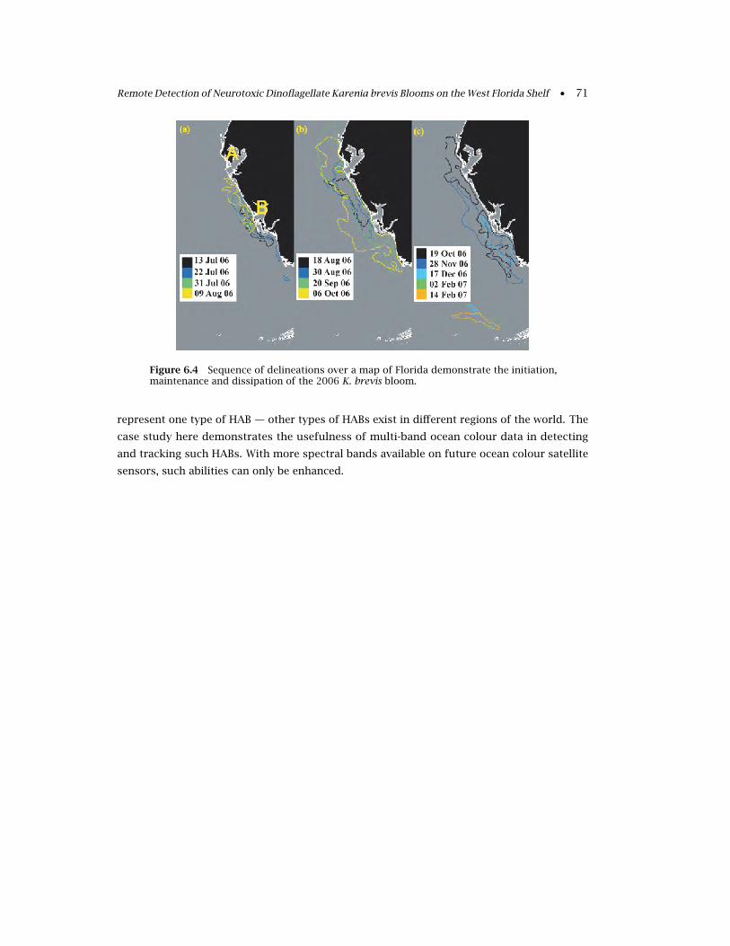
Remote Detection of Neurotoxic Dinoflagellate Karenia brevis Blooms on the West Florida Shelf • 71
Figure 6.4 Sequence of delineations over a map of Florida demonstrate the initiation,maintenance and dissipation of the 2006 K. brevis bloom.
represent one type of HAB — other types of HABs exist in different regions of the world. The
case study here demonstrates the usefulness of multi-band ocean colour data in detecting
and tracking such HABs. With more spectral bands available on future ocean colour satellite
sensors, such abilities can only be enhanced.

72 • Observation of Harmful Algal Blooms with Ocean Colour Radiometry

Chapter 7
Remote Sensing of Cyanobacterial Blooms
Stefan G. H. Simis, Mariano Bresciani, Hongtao Duan, Claudia Giardino, Chuanmin
Hu, Tiit Kutser, Ronghua Ma, Erica Matta and Mark W. Matthews
7.1 Introduction
Cyanobacterial blooms are a familiar sight in freshwater and brackish water bodies near centres
of human activity, posing health and economic threats. A trend of increasing dominance of
cyanobacteria in response to climate change can be shown in lakes (Elliott 2011). Consequently,
water management authorities need targeted monitoring and mitigation efforts, for which
traditional methods to quantify biomass in cell numbers provide insufficient frequency and
spatial coverage. Remote sensing and in situ automated optical monitoring methods therefore
increasingly receive attention. Case studies in this chapter illustrate the feasibility of current
remote sensing techniques to map and distinguish cyanobacteria blooms, covering a wide
geographical range and various trophic states in freshwater and coastal environments.
7.1.1 Terminology, taxonomy, and functional diversity
Cyanobacteria are a diverse group of photosynthetic prokaryotes. They occupy a more primitive
branch in the tree of life than the eukaryotic algae, a fact recognized in the 1970s when the
term ‘blue-green algae’ was abandoned (see Sapp 2005; Govindjee and Shevela 2011). As
a compromise in the otherwise confusing and unpractical naming conventions, the term
phytoplankton is now widely accepted as the collective functional group of photosynthetic
algae and cyanobacteria. Nevertheless, the term (harmful) algal bloom is still freely used in
the remote sensing community to describe proliferations of phytoplankton dominated by
either algae or cyanobacteria, possibly because the dominant phytoplankton group is rarely
determined from remote platforms. It is nevertheless good to bear in mind that deeply
rooted evolutionary and ecophysiological differences between cyanobacteria and algae warrant
consideration when formulating phytoplankton optical models or interpreting remotely sensed
signals.
Cyanobacteria are the most common bloom-forming phytoplankton group in freshwater
bodies, and blooms may additionally form in rivers, estuaries, and coastal seas (Anderson et al.
2002). The most common bloom-forming (planktonic) cyanobacteria are globally represented
by relatively few species from the genera Aphanizomenon, Cylindrospermopsis, Dolichosper-
73

74 • Observation of Harmful Algal Blooms with Ocean Colour Radiometry
mum (including planktonic former Anabaena), Microcystis, Nodularia, and Planktothrix. The
role of (pico)cyanobacteria in primary production in the world oceans is not to be underesti-
mated, but reports of bloom-forming cyanobacteria in the oceans are limited to filamentous
Trichodesmium, which often form dense surface colonies in tropical and sub-tropical oceans,
spanning thousands of square kilometres. Trichodesmium is a nitrogen fixer, and while not
traditionally considered as harmful (thus not discussed in this chapter), interested readers may
refer to a previous IOCCG report (Hu et al. 2014) and a recent review by McKinna (2015) for
detailed information on Trichodesmium optical properties and ocean colour remote sensing
techniques.
The success of cyanobacteria in disturbed environments can be explained by a set of
mechanisms often represented in the most notorious bloom-formers. These mechanisms
are: regulation of buoyancy and pigmentation (discussed below), acclimation of pigment
production (Tandeau de Marsac and Houmard 1988) and rapid acclimation of light utilization
(Papageorgiou et al. 2007; Govindjee and Shevela 2011; Kana et al. 2012), elemental nitrogen
fixation, colony formation either to aid light harvesting (Tamulonis et al. 2011) or to reduce
grazing (Lampert 1987; Chan et al. 2004), poor food quality for higher trophic levels (Lampert
1987) and finally, though subject to debate, allelopathic effects of secondary metabolites
including those toxic to animals (Babica et al. 2006).
Toxicity is the foremost reason to call for early warning of cyanobacteria blooms and
dedicated monitoring, assessment, and remediation strategies in water bodies world-wide.
Effects of cyanobacterial toxins on humans range from skin and respiratory irritation to liver
and kidney damage; excessive exposure has resulted in death (WHO 1999). Public awareness of
the risks of exposure is probably the most efficient preventive strategy for humans, although
recently even living near water bodies where toxin-producing cyanobacteria proliferate was
suggested as a risk factor for degenerative disease such as amyotrophic lateral sclerosis
(Torbick et al. 2014). Meanwhile, livestock, (planktivorous) waterfowl, and pets are particularly
vulnerable to toxins accumulated in surface scums, benthic mats, or in filter feeders (Codd
et al. 1999, 2005).
High-biomass cyanobacterial blooms that can be linked to severe eutrophication are
considered harmful for diverse reasons. New toxins and links to disease are still being
regularly identified (WHO 1999), while blooms that are not toxic can still cause malodour
or skin irritation, reducing the recreational and economic value of affected water bodies.
Further, as with most algal blooms, cascading ecosystem-destabilizing effects can result from
bacteria-mediated oxidation of collapsing blooms, in the worst case leading to mortality of fish
and benthic fauna.
Two aspects of cyanobacterial growth and bloom formation influence our ability to detect
and quantify cyanobacterial biomass using remote sensing, more than any other of the
adaptive mechanisms found in cyanobacteria. These are the relatively unique optical signatures
of cyanobacteria, which allow deterministic detection, and biomass accumulation through
buoyancy regulation. These properties are discussed in more detail, below.

Remote Sensing of Cyanobacterial Blooms • 75
7.1.2 Pigmentation
The most important deterministic optical characteristic of cyanobacteria is the important role
of phycobilipigments in their photochemistry. Phycobilipigments (main forms phycoerythrin,
phycocyanin, and allophycocyanin) are consistently produced in all cyanobacteria except
prochlorophytes. These pigments are the dominant source of photosynthetic light harvesting
in cyanobacteria. Rhodophytes and cryptophytes (including endosymbionts) may also carry
phycobilipigment so the presence of the pigment is not the sole indicator of cyanobacteria.
Figure 7.1 Concentration-specific absorption of dominant cyanobacterial pigmentgroups (thick curves, Simis and Kauko 2012) and major algal pigments (thin curves,Bidigare et al. 1990). C-PC = phycocyanin including absorption by allophycocyanin, C-PE =phycoerythrin, C-Chl-a = Chl-a plus absorption by carotenoid and xanthophyll pigments,Chl-a, Chl-b and Chl-c absorption determined from algae.
Phycobilipigment light absorption is most efficient in the yellow-green part of the visible
light spectrum (Figure 7.1) where chlorophyll, xanthophyll, and carotenoid pigments have
weaker absorption. The distinct absorption of phycocyanin is visible from remote sensors and
has been studied since the 1990s from airborne imagery (Dekker et al. 1991; Dekker 1993;
Jupp et al. 1994), and in bio-optical experiments (Gons et al. 1992; Hunter et al. 2008). In
recent years, a number of empirical and semi-analytical algorithm development studies have
emerged, ranging from the use of two (Schalles and Yacobi 2000; Hunter et al. 2009) to three
or more wavebands (Simis et al. 2005, 2007; Hunter et al. 2010; Le et al. 2011; Sun et al. 2013;
Mishra et al. 2013; Liu et al. 2017; Varunan and Shanmugam 2017) and hyperspectral data
(Kutser 2004). Kutser et al. (2006) demonstrate, through bio-optical modelling, that very few
current satellite sensors can distinguish the diagnostic absorption profile of cyanobacteria.
Nevertheless, cyanobacteria blooms may still be mapped and even quantified using purely
empirical relationships between the limited band sets of Landsat TM (Vincent et al. 2004; Sun
et al. 2015) or the Indian Ocean Color Monitor (OCM) on Oceansat-1 (Dash et al. 2011). Sensor
requirements are discussed in more detail by Kutser (2009), but it is worth noting here that
when the Medium Resolution Imaging Spectrometer (MERIS) sensor on ENVISAT (2002-2012)
became the first spaceborne sensor with global coverage to provide a channel (620 nm) tuned
to phycocyanin, this prompted a marked increase in efforts to make cyanobacterial bloom

76 • Observation of Harmful Algal Blooms with Ocean Colour Radiometry
monitoring from space possible. Several independent algorithm validation efforts have since
demonstrated good retrieval results when cyanobacteria are sufficiently abundant, although
accurate quantification in mixed phytoplankton assemblages often remains challenging (Ruiz-
Verdú et al. 2008; Randolph et al. 2008; Li et al. 2010; Wheeler et al. 2012; Qi et al. 2014). The
MERIS waveband configuration, including several new channels, is continued on the Ocean and
Land Colour Instrument (OLCI) onboard the Copernicus Sentinel-3 series. The main benefit of
these missions is guaranteed continuity, which has prompted the development of operational
cyanobacteria observation systems, such as the examples given in Chapter 10 of this report.
Phycobilipigments are soluble in water, unlike other plant pigments. Chemotaxonomic
methods for pigments extracted in organic solvents are therefore not useful to quantify
phycobilipigments. Alternative extraction methods (e.g., Sarada et al. 1999) have proven
laborious and difficult to standardize. Consequently, the quantification of phycobilipigments
is often based on in vivo optical properties such as fluorescence rather than on the analysis
of extracted pigments. Today, a lack of concurrent observations of the optical properties
and extracted phycobilipigment in bloom situations still hampers pigment-based algorithm
development for remote sensing of cyanobacteria blooms.
The production of the accessory pigments depends both on species and environment
(light intensity, light quality, and nutrient availability). This natural variability should be kept
in mind when using remote sensing algorithms that target accessory pigments to quantify
cyanobacterial biomass. The fraction of cyanobacteria in the phytoplankton assemblage will
also determine the validity of algorithms based on accessory pigments, due to the overlap in
absorption spectra of these diagnostic pigments with other (algal) pigments in the community
(Figure 7.1).
7.1.3 Buoyancy
Risk of harmful or nuisance cell concentrations increases dramatically when cells accumulate
near the water surface. Mechanisms of buoyancy regulation include formation and collapse of
gas vesicles and changes in cell density. Even neutrally-buoyant species may show a circadian
migration if nutrient and light conditions are inversely stratified and wind-mixing is weak
(Walsby 1994; Visser et al. 2005). Vertical mixing velocity and depth of the mixed layer play a
crucial role in whether buoyancy-regulating species accumulate at the water surface (Wynne
et al. 2010).
Near-surface accumulation increases areal light absorption and scattering by particles.
With increasing near-surface light scattering, near infra-red (NIR) reflectance increases as the
intensity of back-scattered light becomes larger than the strong light absorption by water
itself, up to the point where it resembles the spectral albedo of land vegetation. This effect is
simulated in Figure 7.2 for a fixed biomass of Microcystis cells mixed over different depths
from the surface, a problem previously also addressed for various depth distributions by
Kutser et al. (2008). The strong NIR reflectance of surfacing blooms is relatively easy to identify
from satellite imagery using red and NIR bands (Hu et al. 2010), even without fully correcting
for atmospheric effects on the remotely sensed signal (Matthews et al. 2012). It is therefore

Remote Sensing of Cyanobacterial Blooms • 77
possible to use remote sensing techniques to map the risk of accumulated cyanobacterial
toxins by focusing exclusively on (near) surface blooms.
Figure 7.2 Simulated remote-sensing reflectance of a bloom with the optical propertiesof Microcystis with a fixed areal biomass (200 mg m−2) mixed in a layer up to 0.5 to 20m depth. Near-surface backscattering increases with shallower mixing depth (visible inthe NIR). Spectra were simulated using Hydrolight with fixed IOPs for non-phytoplanktoncomponents (1.8 g m−3 tripton, absorption at 440 nm = 0.05 m−1; CDOM absorption at440 nm = 1 m−1, default water absorption), and sun at zenith with the default atmosphericparameters. Image credit: Mark Matthews and Lisl Robertson.
Atmospheric correction of the water-leaving radiance is strongly affected by increased
reflectance in the NIR region. Misclassification of water pixels as land can be observed
(Matthews et al. 2010), and a general reduction of the accuracy of atmospherically-corrected
reflectance is common (see Baltic Sea case study, Section 7.5). This problem is evident even
when buoyant blooms are only present at sub-pixel scales. Additional sources of information
such as weather-based mixing models, may be used to predict the possibility of surfacing
blooms of buoyant cells. Increased near-surface heat trapping in dense (near) surface layers
can also reveal blooms in maps of sea surface temperature (Kahru et al. 1993).
The effects of near-surface accumulation on cell physiology are commonly ignored in
remote sensing studies. Species of cyanobacteria have been shown to rapidly acclimate to
fluctuating light intensities by redistributing antenna pigments between photosystems (‘state
changes’), effectively reducing their photosynthetic absorption-cross section (e.g., Papageorgiou
et al. 2007; Govindjee and Shevela 2011; Kana et al. 2012). Under prevailing intense light
exposure, cells will favour production of photoprotective rather than photosynthetic pigment.
In situ observations of changes in the optical properties of cyanobacteria are lacking, probably
due to the difficulties in sampling surface blooms without disturbing them. We may, however,
expect that surface accumulations observed during calm days require different absorption
terms for cyanobacteria compared to well-mixed conditions.
The case studies presented in this chapter include studies on lakes and the brackish Baltic
Sea. The densest blooms occur in eutrophic lakes where the optical signatures of cyanobacteria
can dominate the water-leaving radiance. The use of state-of-the-art sensors, long time series
from remote sensors, and optical proxies of biomass in oligotrophic to hyper-eutrophic waters
are demonstrated. Cyanobacteria blooms in the marine sphere are used to further demonstrate
the effects of spatial and temporal resolution on the retrieval of patchy blooms and time series,
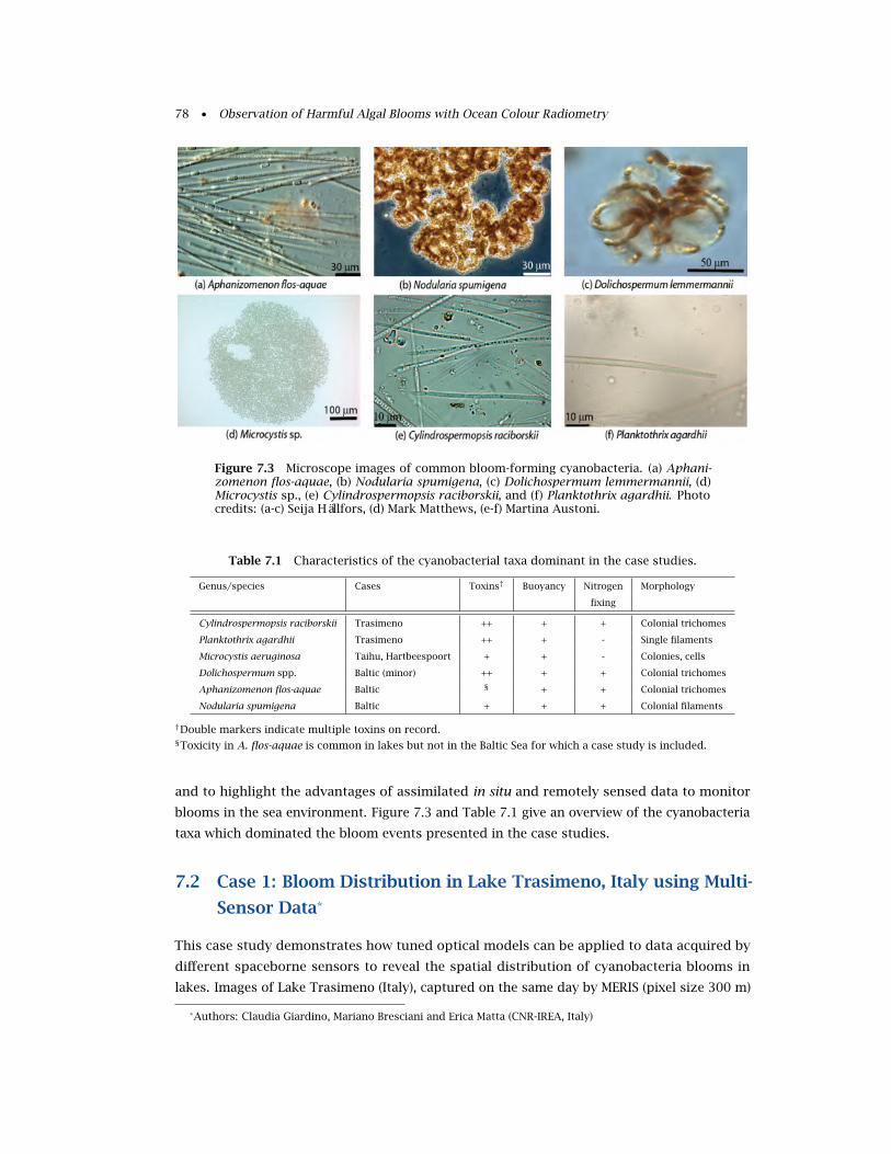
78 • Observation of Harmful Algal Blooms with Ocean Colour Radiometry
Figure 7.3 Microscope images of common bloom-forming cyanobacteria. (a) Aphani-zomenon flos-aquae, (b) Nodularia spumigena, (c) Dolichospermum lemmermannii, (d)Microcystis sp., (e) Cylindrospermopsis raciborskii, and (f) Planktothrix agardhii. Photocredits: (a-c) Seija Hällfors, (d) Mark Matthews, (e-f) Martina Austoni.
Table 7.1 Characteristics of the cyanobacterial taxa dominant in the case studies.
Genus/species Cases Toxins† Buoyancy Nitrogen Morphology
fixing
Cylindrospermopsis raciborskii Trasimeno ++ + + Colonial trichomes
Planktothrix agardhii Trasimeno ++ + - Single filaments
Microcystis aeruginosa Taihu, Hartbeespoort + + - Colonies, cells
Dolichospermum spp. Baltic (minor) ++ + + Colonial trichomes
Aphanizomenon flos-aquae Baltic § + + Colonial trichomes
Nodularia spumigena Baltic + + + Colonial filaments
†Double markers indicate multiple toxins on record.§Toxicity in A. flos-aquae is common in lakes but not in the Baltic Sea for which a case study is included.
and to highlight the advantages of assimilated in situ and remotely sensed data to monitor
blooms in the sea environment. Figure 7.3 and Table 7.1 give an overview of the cyanobacteria
taxa which dominated the bloom events presented in the case studies.
7.2 Case 1: Bloom Distribution in Lake Trasimeno, Italy using Multi-
Sensor Data*
This case study demonstrates how tuned optical models can be applied to data acquired by
different spaceborne sensors to reveal the spatial distribution of cyanobacteria blooms in
lakes. Images of Lake Trasimeno (Italy), captured on the same day by MERIS (pixel size 300 m)
*Authors: Claudia Giardino, Mariano Bresciani and Erica Matta (CNR-IREA, Italy)

Remote Sensing of Cyanobacterial Blooms • 79
and CHRIS-PROBA (pixel size 18 m), are compared. MERIS was operational on ESA’s Envisat
satellite for more than 10 years and is still used for retrospective analysis and algorithm
development, whereas the OLCI sensors on Sentinel-3A and-B, with similar spectral and
radiometric characteristics, have been operational since 2016/2018 respectively. CHRIS, on the
PROBA platform, is a hyperspectral instrument and provides a limited number of daily scenes.
7.2.1 Study area
Lake Trasimeno, the fourth largest lake (124 km2) in central Italy (43°06’N; 12°07’E), is a closed,
unstratified, and shallow lake (average depth 4.5 m, maximum depth 6 m), and was declared a
protected area for its exceptional natural value (Directive CEE 1979). Tourism, agriculture and
livestock breeding are the most important activities in the Trasimeno area. The annual load of
organic carbon (500t), nitrogen (550t) and phosphorus (30t), negatively affects water quality
(Cingolani et al. 2005): cyanobacteria blooms are present, sediments negatively impacted,
the fish community altered and common reeds are in recession (Natali 1993; Cecchetti and
Lazzerini 2007; Cingolani et al. 2007).
Cylindrospermopsis raciborskii and Planktothrix agardhii dominate the phytoplankton in
late summer with cell densities reaching 2–3×10⁷ and 2–5×10⁶ l−1, respectively (Cingolani
et al. 2007; Lucentini and Ottaviani 2011). Mycrocystis aeruginosa is also common. Blooms
occur in the water column and at the surface, but scum is rarely observed. Field data of
August 2011 confirm elevated cyanobacteria biomass, mainly in the lake centre, with Chl-a
concentration values around 40 mg m−3. During the bloom, on 19 August 2011, MERIS and
CHRIS-PROBA data were acquired near-simultaneously.
Figure 7.4 MERIS FR and CHRIS-PROBA comparison of remote-sensing reflectance (Rrs)averaged over the central area of Lake Trasimeno on 19 August 2011. Dotted linesshow minimum and maximum values. Reflectance depressions caused by cyanobacteriapigments are visible in the orange-red range.

80 • Observation of Harmful Algal Blooms with Ocean Colour Radiometry
7.2.2 Image processing
MERIS full resolution and CHRIS-PROBA images acquired on 19 August 2011 were processed
using BEAM tools (Fomferra and Brockmann 2006) to normalise radiometric noise at satellite
level (smile correction for MERIS, noise reduction for CHRIS-PROBA). The TOA radiance was
corrected for atmospheric effects using the 6S code (Vermote et al. 1997; Kotchenova et al.
2006). The 6S-derived reflectances obtained from MERIS and CHRIS-PROBA were comparable
both in magnitude and shape (Figure 7.4), confirming the accuracy of the absolute radiometric
properties of both sensors over the central area of the lake. The spectral shapes of the
reflectance, with reflectance minima near pigment absorption peaks in the blue and red, and
the peak at 709 nm indicates a strong influence by phytoplankton on the signal. The depression
of the reflectance signal in the 620 nm band suggests the presence of cyanobacteria-specific
pigments. Water reflectances were transformed into Chl-a concentrations with the BOMBER
optimization technique (Giardino et al. 2012). BOMBER hosts a three-component bio-optical
model that was parameterised with optical coefficients suitable for Lake Trasimeno.
Figure 7.5 Lake Trasimeno images acquired on 19 August 2011. (a) Pseudo true colourMERIS image of Lake Trasimeno (north) and Lake Bolsena (south). The image clearlyshows the different appearance of these lakes. (b) MERIS (R:G:B = 620:560:442 nm) and(c) CHRIS-PROBA (R:G:B = 620:560:441 nm) images of Lake Trasimeno at the same scale;both images show the green hue of Lake Trasimeno waters affected by phytoplanktonbloom. Chl-a concentration from (d) MERIS, and (e) CHRIS-PROBA images (colour scale0-50 mg m−3 from blue to red).

Remote Sensing of Cyanobacterial Blooms • 81
7.2.3 Results and discussion
The intense green appearance of Lake Trasimeno observed in pseudo-true colour images (Figure
7.5, visible in the north) contrasts sharply with the clear waters of Lake Bolsena (south-west),
a deep oligotrophic volcanic crater lake. Both MERIS (Figure 7.5b) and CHRIS (Figure 7.5c)
coverage of Lake Trasimeno also highlight a contrast within the lake: cyanobacterial blooms
cause the intense green hues, while submerged macrophyte beds in the southeast corner
regulate water transparency, resulting in clear waters. Wind resuspension of sediments on 19
August 2011, with average wind speed 8 m s−1 and peak wind of 15 m s−1, resulted in variable
patterns of brightly scattering waters along the eastern lake shore. Maps of Chl-a concentration
obtained with BOMBER (Figure 7.5d-e) show generally good correspondence, although the
higher resolution of the CHRIS-PROBA image reveals many finer structures. The two images
do not correspond well along the northern shore, and in particular in the southeast corner
of the lake. This is probably due to the adjacency effects that can alter the signal originating
from the water column due to the multiple-reflection of radiation from the surrounding lands
(Guanter et al. 2010). The adjacency effect also depends on pixel size and hence it causes
different patterns in the two images.
This study shows that different satellite sensors can be used to map Chl-a concentration
in lakes where well-calibrated and validated physics-based approaches are available for the
study area. The approach used in this study was based on 6S and BOMBER: the first code
was used to convert MERIS and CHRIS-PROBA radiances into water reflectance. BOMBER, in
turn, was parameterised with the optical properties of Lake Trasimeno, and used to derive
Chl-a concentration, which, for this study area, can be assumed to delineate cyanobacteria
biomass. The results show that MERIS and CHRIS-PROBA can be used to produce realistic and
reproducible reflectance spectra. The Chl-a concentration patterns assessed from space reveal
that, even in medium sized lakes, the horizontal variability warrants the use of remote sensing
to complement point sampling.
7.3 Case 2: Lake Taihu, China†
Long-term studies of phytoplankton blooms in lakes and estuaries are extremely rare in remote
sensing literature, due to the inherent problems in atmospheric correction and bio-optical
inversion in waters where sediments and other non-living constituents can play dominant
optical roles. This case study demonstrates that satellite sensors, even those not optimized
for lake water quality remote sensing, can be used to derive meaningful descriptions and
long-term patterns of extreme cyanobacterial blooms.
Lake Taihu, the third largest freshwater lake in China with a surface area of 2,338 km2 and
average water depth of 1.9 m, is one of the most severely polluted freshwater reservoirs in
China (Figure 7.6). In May 2007, a massive bloom of Microcystis aeruginosa disrupted water
supply to Wuxi city leaving over 1 million people without drinking water for a week. The
†Authors: Chuanmin Hu1, Hongtao Duan2, Ronghua Ma2 (1University of South Florida, USA; 2Nanjing Institute of
Geography and Limnology, Chinese Academy of Sciences)

82 • Observation of Harmful Algal Blooms with Ocean Colour Radiometry
extreme bloom event placed Lake Taihu in the spotlight (Guo 2007; Yang et al. 2008; Qin
et al. 2010) and inspired increased focus on studies and management of the eutrophication
problems that affect water quality in the lake.
Figure 7.6 Location of Lake Taihu in China. The cities of Wuxi and Suzhou are locatedto the Northeast and East of the lake, respectively. The lake is divided into segmentsbased on morphology and hydrodynamics. Figure adapted from Duan et al. (2009).
7.3.1 Image processing and analysis
MODIS 250-m resolution and Landsat TM/ETM 30-m resolution images are used. MODIS Level-0
(raw digital counts) data from both Terra and Aqua satellites were obtained from the NASA
Goddard Flight Space Center (GSFC). Landsat data include nearly all cloud-free images over
Lake Taihu since 1987, and were provided by the United States Geological Survey (USGS) and
China Remote-Sensing Satellite Ground Station (Duan et al. 2009; Hu et al. 2010). Due to
the 16-day revisit time, Landsat images were used to identify when blooms initially occurred
up until the year 2000. From the year 2001 onwards, MODIS Level-0 data were converted to
calibrated radiance data using the software package SeaDAS (version 5.1). Gaseous absorption
and Rayleigh scattering were corrected using software provided by the MODIS Rapid Response
Team, based on the radiative transfer calculations from 6S (Vermote et al. 1997). The resulting
Rayleigh-corrected reflectance data, Rrc(λ) where λ is the central wavelength of the bands,
were geo-referenced to a cylindrical equidistance (rectangular) projection (errors less than 0.5
pixel). Landsat data were processed in a similar fashion to the MODIS scenes.
When the water surface is calm under low wind, buoyant cyanobacteria cells form floating
mats (scums) at the surface. Under these circumstances the Floating Algae Index (FAI, Hu 2009)
is sensitive to the presence of buoyant cyanobacteria in the lake. FAI is defined as (Hu 2009;
Hu et al. 2010):
FAI = Rrc(λ1)− R′rc(λ1)
R′rc(λ1) = Rrc(λ2)+ (Rrc(λ3)− Rrc(λ2))× (λ1 − λ2)/(λ3 − λ2)(7.1)
For MODIS, the wavebands used to generate the FAI were λ1 = 859 (841–876) nm, λ2 = 645

Remote Sensing of Cyanobacterial Blooms • 83
(620–670) nm, and λ3 = 1240 (1230–1250) nm. With Landsat, the bands used were λ1 =
825 (750–900) nm, λ2 = 660 (630–690) nm, and λ3 = 1650 (1550–1750) nm. The FAI detects
the red-edge of reflectance of surface vegetation (in this case, cyanobacteria bloom mats).
Basically, FAI quantifies the surface reflectance in the NIR normalized against a baseline formed
linearly between the red and short-wave infrared (SWIR) wavebands. FAI values > -0.004 were
empirically established to delineate blooms (Hu et al. 2010).
Figure 7.7 Initial outburst date for lake Taihu blooms through the time-period 1987–2011. Regression lines for specific periods: 1987–1997: y = 5.35x − 10473 (r 2 = 0.56);1997–2007: y = −9.84x + 19844 (r 2 = 0.57); 2007–2011: y = 11.8x − 23596 (r 2 = 0.96).Figure adapted from Duan et al. (2014).
Several lake segments (Gong Bay and East Lake, see Figure 7.6) have seasonal water plants
(Ma et al. 2008) which may appear as blooms but should be interpreted as mixed plants and
phytoplankton. The seasonal cycle of East Bay is almost purely from water plants. Results
labelled to represent the whole lake should be interpreted as Lake Taihu excluding East Bay.
Temporal dynamics of the bloom are described using two indicators: the initial blooming
date and bloom duration. The initial blooming date is the first date of each year when blooms
could be discerned by visual inspection of the Landsat and MODIS FAI and Red-Green-Blue
imagery. Blooms occurred every year in the observed period, although the years 1988 and 1999
had to be excluded due to lack of sufficient imagery. Three distinct trends in the initial bloom
date were observed (Figure 7.7); from 1987 to 1997, the blooms appeared with an increasing
delay of 5.35 days per year. From 1997 to 2007, blooms started increasingly earlier by 9.83
days per year. Since 2007, blooms have again started to appear later with a delay of 11.8 days
per year.
Bloom duration is defined as the period between first and last appearance in MODIS FAI
imagery. More than one bloom may occur in any period. The bloom duration is mapped for
the years 2000–2011 in Figure 7.8. The period 2006–2011 showed longer bloom duration in
most of the lake compared to the years prior, despite later starts to the bloom (Figure 7.7).
The trend actually began in 2005, with 2007 being the worst bloom year. More than half the
lake surface had blooms lasting for > 7 months during 2007. Earlier and longer blooms in the
period 2007–2011 are apparent for NW Lake, SW Lake, Central Lake, and the whole lake. Bloom

84 • Observation of Harmful Algal Blooms with Ocean Colour Radiometry
Figure 7.8 Duration of cyanobacteria blooms, defined as the period between the firstand last day with FAI > -0.004 in MODIS imagery. White areas showed no bloom duringthe entire year. Figure adapted from Hu et al. (2010).
coverage never exceeded 25% of the lake area between 2000 and 2003, and exceeded 25% of
the lake area only twice during 2004 when the entire lake was considered. This suggests that
the lake was relatively healthy between 2000 and 2004.
7.3.2 Spatial patterns
Besides time-series analysis, the archive of bloom imagery can also be used for spatial analyses,
such as where blooms initiate and how they expand. Blooms were first observed in Meiliang
Bay and Gonghu Bay in June, 1987. Throughout the past two decades, the initial bloom location
was Meiliang Bay (14 times) and Zhushan Bay (9 times) — on four of these occasions, blooms
occurred simultaneously in both locations. Since 2000, blooms have also started to spread
from western and southern bays, which may indicate changes in the hydrodynamic regime or
nutrient delivery to the lake. The blooms show a sprawling trend, covering an increasing area
from year to year. The bloom area increased from 4.8 km2 in July 1991 to 216.4 km2 in 2000,

Remote Sensing of Cyanobacterial Blooms • 85
and the extreme situation in 2007 when blooms covered > 1,000 km2.
For most lake areas (NW Lake, SW Lake, Central Lake) as well as when considering the entire
lake, 2005 marks a transition year from relatively rare bloom occurrence to highly frequent
blooms (high FAI in > 25% of the area), particularly during summer months.
Apr 4, 2007 Apr 11, 2007 Apr 18, 2007
Apr 20, 2007 May 19, 2007 Jul 11, 2007
Aug 30, 2007 Nov 21, 2007 Jan 5, 2008
Figure 7.9 Initiation and evolution of the 2007 cyanobacteria bloom in Lake Taihu.Figure adapted from Hu et al. (2010).
The 2007 bloom event in Lake Taihu, and particularly Meiliang Bay, was reported to start
in late April (Yang et al. 2008) and by 25 April extensive blooms were found in Meiliang Bay
(Kong et al. 2007). The MODIS FAI image series of 2007 (Figure 7.9) reveals that an extensive
bloom was already established on 4 April 2007 in NW Lake and SW Lake, three weeks earlier
than reported as the onset of the bloom. By 18 April, the bloom was already extensive in
Meiliang Bay, again a week earlier than reported. Between 20 April and 30 August, the bloom
covered almost the entire Meiliang Bay. On 11 July and 21 November, more than half of the
entire lake was covered by the intense bloom, which remained until at least 5 January 2008,
making it the longest bloom event since MODIS data became available (2000) and possibly
the longest bloom event in history. In June 2007, at least 6000 tons of organic material was
harvested from the bloom in an attempt to reduce the bloom (Guo 2007). The remotely sensed
imagery suggests, however, that the impact of this effort on bloom size was limited.

86 • Observation of Harmful Algal Blooms with Ocean Colour Radiometry
7.3.3 Factors forcing blooms
7.3.3.1 Temperature
Cell recruitment in Lake Taihu has been shown to be tightly coupled to temperature, both in the
laboratory and in the field (Cao et al. 2008). The initial blooming date calculated from MODIS
imagery was significantly correlated to the minimum water temperature during the preceding
winter (November–January, p = 0.048). The winter of 2007 was one of the warmest winters in
the previous 25 years, particularly in the period January–March (0.36, 2.78, and 1.98°C above
average in January, February, and March, respectively). The elevated water temperatures may
have supported the extreme bloom of that year. If minimum winter temperature is indeed a
driving force behind recruitment and bloom formation, current trends of increasing minimum
temperature (at a rate of 0.0539°C yr−1) suggest further bloom expansion in years to come.
7.3.3.2 Nutrients
Nutrient loading resulting from human activities contributes to the blooms in Lake Taihu.
During the period 1991–1996, the annual average total nitrogen (TN) increased from 1.18 mg
l−1 to 3.62 mg l−1, total phosphorus (TP) increased from 0.10 mg l−1 to 0.18 mg l−1. By 2006,
TN and TP were 200% and 150% higher than in 1996 (Kong et al. 2007). Nutrient analysis
at Taihu field station showed that inputs of TN and TP from the catchment area increased
by 3 and 5%, respectively, between 2002 and 2003 (Kong et al. 2007). The spatial patterns
displayed by the blooms support the hypothesis that nutrient availability drives the blooming.
The southward expansion of the blooms reflects the higher nutrient loading northwest of Lake
Taihu. For example, TP loading from the northwest catchments accounted for 53–55% of the
entire area in the period 2002–2003, and TN loading from this area accounted for 65–72% in
2002–2003. The southward delivery of nutrients explains the frequent occurrences of blooms
in the north, and increasing detection of blooms in the center and south.
7.3.3.3 Wind
Despite the shallow average depth of Lake Taihu, wind mixing can have a large effect on the
appearance of floating cyanobacteria mats. During days with consecutive MODIS imagery in
September 2005 and November 2007, bloom size was observed to be as large as > 770 km2
for wind speed < 2 m s−1 but reduced to < 140 km2 for wind speed > 3 m s−1. It is unlikely
that an extensive bloom could disappear in one day and a new bloom initiate immediately
thereafter. Therefore, the observed oscillation in bloom size over consecutive days must be
due to changes in physical conditions (primarily wind forcing), and not due to changes in the
total biomass.
7.3.3.4 Economic prosperity
The combined pressures of land use (sewage, livestock, drainage, soil nutrients and loss of
fertilizers from agricultural lands (see Lai et al. 2006) on the lake ecosystem can be associated

Remote Sensing of Cyanobacterial Blooms • 87
with human population and economic development. Human population and the gross domestic
product (GDP) per capita were used to explore the correlation of anthropogenic activities with
phytoplankton blooms. Including these factors as well as winter temperature in a multivariate
regression shows that GDP and GDP per capita are the best predictors of bloom occurrence:
GDP was the dominant factor for the initial blooming date (r 2 = 0.988), while GDP per capita has
the strongest relation with bloom duration (r 2 = 0.747). These findings imply that economic
activities outweigh the environmental effect of the preceding winter temperature despite the
fact that temperature does explain the variability of the bloom initiation dates.
GDP in the Taihu Basin increased from 847.66 to 2,662.23 billion Yuan (RMB) from 1998 to
2007. GDP per capita increased from 2.06 ×10⁴ to 6.16×10⁴ Yuan (RMB). Correspondingly,
the number of months of detected algal blooms increased from two in 1998 to ten in 2007;
the initial blooming date advanced more than 100 days. Significant correlations were found
between the annual duration, initial blooming date and total GDP, and GDP per capita in the
adjacent area for the time period of 1998–2007. Human activity is projected to further grow in
this area in the next decades.
7.3.4 Discussion
The Taihu case shows that a reflectance band index such as FAI can delineate cyanobacterial
bloom mats at the water surface due to the associated dominant NIR optical feature. This
approach is valid even without the use of rigorous atmospheric correction and bio-optical
inversion algorithms. Unlike algorithms which target the absorption feature of phycocyanin
around 620 nm in mixed conditions, and available from a limited number of satellite sensors,
FAI uses a NIR band to quantify surface mats of buoyant cyanobacteria. The surface mats show
spectral characteristics similar to surface vegetation. At the time of writing, both MODIS-Terra
(2000 to present) and MODIS-Aqua (2002 to present) are functional, and Landsat-8 (February
2013 to present) and Landsat-9 (scheduled for mid-2021) continue the Landsat series to provide
Earth science data. Thus, the time-series analysis can be continued to assess bloom conditions
in the coming years. Even if both MODIS instruments stop functioning (both were designed to
have a 5-year mission life), the Visible Infrared Imager Radiometer Suite (VIIRS) instrument on
Suomi NPP (National Polar-orbiting Partnership) satellite (October 2011 to present) is expected
to provide continuity of the bloom observations. VIIRS is equipped with several imaging and
ocean colour bands in the red, NIR, and SWIR that are suitable to derive the FAI, as with MODIS.
Alternatively, the Landsat-8 OLI sensor with 30-m spatial resolution has suitable red, NIR, and
SWIR bands and improved signal-to-noise ratios compared to its predecessors (Hu et al. 2012;
Pahlevan et al. 2014). The uninterrupted observations from these environmental satellites will
provide seamless data records to assure data continuity to assess the long-term bloom status
in Lake Taihu and similar water bodies under heavy pressure.
The results obtained from satellite-based observations are not only useful in understanding
the potential causes of the blooms and their long-term trends, but also useful to aid decision-
making. For example, the statistics of the spatial and temporal bloom patterns can help
management agencies in implementing nutrient release and reduction plans. The timely

88 • Observation of Harmful Algal Blooms with Ocean Colour Radiometry
information from the near real-time satellite images can help local groups to determine where
to harvest scums to improve water quality. Currently, at the Nanjing Institute of Geography and
Limnology (China), the MODIS and Landsat-based observations are being integrated with other
information (wind, field observations, temperature) to establish a bloom monitoring system,
with the ultimate goal of predicting bloom occurrence and helping water quality management.
Continuous satellite observations will play an essential role in such a system.
7.4 Case 3: Detecting Trophic Status, Cyanobacteria Dominance, and
Surface Scums in Lakes‡
This case study illustrates retrieval of quantitative bloom biomass over a wide trophic range.
Issues with image quality over severe blooms and near land masses are tackled by using
bottom-of-atmosphere radiance rather than signals corrected for the full atmosphere. Biomass
can be quantified using a series of empirical algorithms that use the shape of the red to near
infra-red (NIR) radiance spectrum. The choice of algorithm is based on a decision tree that
separates clear and turbid waters from those where surface blooms or vegetation are present.
Trophic status remains a crucial variable in water management, and its detection from
satellite provides a unique opportunity, especially in the developing world where information
on water quality is often difficult to obtain. The identification of high biomass cyanobacterial
blooms and their changes in space and time is another major priority for water and public
health management. Despite the high impact and great opportunity presented by Earth
observation from space, there has been an absence of simple, reliable information products for
trophic status and cyanobacteria detection in inland and eutrophic waters. The development
of algorithms targeted at filling this information gap has now become a priority for scientists
and space agencies. This case study demonstrates how the Maximum Peak Height (MPH)
algorithm (Matthews et al. 2012) can be used to provide trophic status, surface scum and
floating vegetation (macrophyte) detection in a variety of South African and global inland
waters. It also demonstrates a pixel flagging process aimed at identifying high-biomass (Chl-a
> 20 mg m−3) cyanobacterial blooms using the full resolution (FR) data archived from Envisat
MERIS.
7.4.1 The MPH algorithm
Detection of Chl-a concentration and other water constituents commonly follows interpretation
of water-leaving reflectances, which are obtained after atmospheric correction of top-of-
atmosphere (TOA) radiances. However, atmospheric correction is challenging and error-prone
over optically complex water types which contain high and uncoupled concentrations of
various constituents (Guanter et al. 2010). While atmospheric effects caused by aerosols (dust,
particles, and smoke) are highly variable and stochastic, Rayleigh or molecular scattering
can be corrected for relatively easily. The Bottom-of-Rayleigh (BRR) processor in the Envisat
‡Author: Mark Matthews — CyanoLakes (Pty) Ltd, South Africa

Remote Sensing of Cyanobacterial Blooms • 89
BEAM software was used to produce the Rayleigh-corrected TOA imagery used with the MPH
algorithm. The band ratio type algorithm used by MPH subsequently normalises remaining
aerosol effects.
The MPH algorithm utilises the signal derived from phytoplankton pigments, fluorescence,
and backscattering in the red/NIR bands of MERIS (for a full description see Matthews et al.
2012). These features may be detected using the Rayleigh corrected TOA signal (e.g., Giardino
et al. 2005). The algorithm uses a baseline-subtraction procedure (see Gower et al. 1999a) to
derive the height of the peak of the MERIS bands between 664 and 885 nm. The three peaks
are centred on phytoplankton Chl-a fluorescence (681 nm), the particulate scattering and water
absorption induced peak (709 nm), and the red edge vegetation band (754 nm). Three cases
are targeted by this technique (see Figure 7.10):
1. mixed oligo-mesotrophic waters with eukaryotic phytoplankton (algae);
2. high biomass eutrophic/hypertrophic waters with either algae or cyanobacteria;
3. extremely high biomass blooms of algae or cyanobacteria with surface scum or floating
vegetation.
Figure 7.10 BRR spectra showing reflectance features applicable to each trophicclass/water type: (1) mixed oligo-mesotrophic waters with eukaryotic phytoplank-ton possessing a Chl-a fluorescence signal at 681 nm (arrow 1) (2) high biomass eu-trophic/hypertrophic waters with (2A) algae and (2B) cyanobacteria, and cyanobacteriawith surface scum (3A), extremely high biomass blooms of algae (3B), and floating vegeta-tion (3C). The arrows 2 and 3 indicate the reflectance features used to identify waters ascyanobacteria dominant (only present in spectra 2B and 3A). Figure credit Mark Matthews.
In each trophic case, MPH exploits a different signal source. In the first case, the Chl-a
fluorescence signal at 681 nm is correlated to biomass and provides information on trophic
state at low-medium biomass with Chl-a < 20 mg m−3 (e.g., Giardino et al. 2005). This signal
becomes masked by particulate absorption and scattering as biomass increases. The second
case utilises the backscattering/absorption induced peak around 709 nm, which is highly
correlated with algae and cyanobacterial biomass at higher trophic states (Chl-a > 20 mg m−3)
(e.g., Gitelson 1992). The final case utilises the vegetation red-edge which becomes apparent in

90 • Observation of Harmful Algal Blooms with Ocean Colour Radiometry
surface scum conditions (Chl-a greater than ∼300 mg m−3) and is characteristic of floating
vegetation with minimal water absorption (Figure 7.2, Kutser 2009). The MPH variable is
designed to seamlessly shift between these cases which occur in inland waters, providing an
operational algorithm for effective trophic status determination through estimates of Chl-a
concentration.
Figure 7.11 a) Empirical algorithms derived from the MPH variable using data fromeutrophic eukaryote dinoflagellate/diatom dominant waters and hypertrophic cyanobac-teria (Microcystis) dominated waters. (b) Algorithm performances over several trophicclasses. From Matthews et al. (2012), reprinted with permission from Elsevier.
The detection of waters dominated by high biomass blooms of cyanobacteria uses re-
flectance features produced by their unique pigmentation. These are an apparent absence
of Chl-a fluorescence causing a trough near 681 nm, and a small peak at 664 nm caused by
sparse pigment absorption (potentially enhanced by phycobilipigment fluorescence) and the
absorption of phycocyanin at 620 nm. These reflectance features are used together to flag
pixels as cyanobacteria dominant water, as seen in Figure 7.11.
7.4.2 Detection of eukaryote and cyanobacteria dominated waters
The MPH variable (the height of the peak in the red/NIR) is proportional to backscattering
from phytoplankton as long as phytoplankton is the dominant optically-active constituent.
The concentration of Chl-a is strongly linearly correlated to phytoplankton backscattering on a
species-specific basis (Whitmire et al. 2010). If the backscattering to biomass ratio between
species or bloom types is sufficiently large, distinct relationships between the MPH variable
and Chl-a concentration can be defined and used for diagnostic bloom detection. The MPH
algorithm was calibrated to two data sets: one from eutrophic eukaryote dinoflagellate/diatom
dominated waters, and one from hypertrophic waters dominated by Microcystis (Figure 7.11).
MPH in the Microcystis-dominated waters was almost an order of magnitude higher than the
eukaryotic blooms, likely owing to small size and the presence of gas vacuoles (Matthews

Remote Sensing of Cyanobacterial Blooms • 91
and Bernard 2013). This result supports the use of MPH to identify high-backscattering
cyanobacteria species such as Microcystis.
Figure 7.12 Chl-a concentration maps derived from MERIS FR imagery of HartbeespoortLake during (a) clear (oligotrophic) and (b) hypertrophic phases. Cyanobacteria dominantpixels are shaded and surface scum is dark green. (c) A 10-year time series of Chl-aconcentration, cyanobacteria coverage, and surface scum coverage of the lake, based onthe full MERIS FR archive. Figure credit Mark Matthews.
Application of the MPH algorithm in Hartbeespoort Lake shows the detection over time
of trophic status, cyanobacteria, and surface scum accumulations (Figure 7.12). The lake
is dominated by spring outbreaks of Microcystis which persist well into autumn and only
occasionally disappear in winter as the water cools. The mean Chl-a concentration regularly
reaches 500 mg m−3 in summer and spring, and may be as high as 1,000 mg m−3 (the limit
assigned to the algorithm). The bloom phenology (initiation and persistence) is strongly
seasonal. Cyanobacteria are dominant over the majority of the lake surface area for most
of the year, with only a temporary respite during winter months, with the exception of a
prolonged clear phase observed during the winter and spring of 2005 and 2011. This clear
phase may be a result of mitigation measures to reduce eutrophication in the reservoir, or
from interannual variations in weather. Surface scum (defined by Chl-a > 500 mg m−3) are

92 • Observation of Harmful Algal Blooms with Ocean Colour Radiometry
frequent during spring and summer months and cover large areas of the lake.
7.5 Case 4: Summer Blooms in the Baltic Sea§
7.5.1 Objective
This case study demonstrates the use of remote sensors to follow the seasonal development of
the typical summer bloom of filamentous cyanobacteria in the Baltic Sea. Bloom biomass is in
the order of 4–10 mg Chl-a m−3 under well-mixed conditions. Diagnostic pigment absorption
features are therefore not quantifiable from remotely sensed imagery. Under calm weather,
however, buoyant species can accumulate near the water surface. This phenomenon enhances
the distinct optical signatures of cyanobacterial pigment absorption, but simultaneously
degrades the performance of atmospheric correction procedures. A highly patchy distribution
of the bloom introduces significant sub-pixel variation, increasing the uncertainty in the quality
of quantitative remote sensing products. These uncertainties stress the need for careful
interpretation of image quality and illustrate the added value of data assimilation with in situ
observations.
7.5.2 Study area
The Baltic Sea is a eutrophic coastal sea with limited water exchange with the North Sea, high
nutrient input, and summer stratification supporting cyanobacteria-dominated phytoplankton
populations when temperatures increase and inorganic nitrogen-phosphorous ratios decrease.
Summer blooms commonly include the filamentous Aphanizomenon flos-aqua, Nodularia
spumigena, and Dolichospermum spp. and occur naturally (Niemi 1973; Leppänen et al. 1995;
Bianchi et al. 2000).
The peak period of cyanobacteria growth is around mid-July, although A. flos-aqua is
found in low densities in all seasons. The rate of bloom development depends on nutrients
available after the spring bloom (up to 50 mg Chl-a m−3) and on water temperature. Summer
cyanobacterial bloom biomass is typically in the range 4–10 mg Chl-a m−3. Under calm
conditions, the filamentous species rise to the surface and locally accumulate higher biomass.
Water samples taken from ships tend to disturb near-surface stratified layers, so measured
concentration ranges do not typically represent such situations.
7.5.3 Image analysis: Delineating blooms
Phytoplankton are the dominant source of light scattering in the open Baltic Sea during bloom
periods and away from river plumes and shallow areas. Deriving maps of phytoplankton
biomass in the open sea can therefore be as straightforward as extracting the dominant
optical signal from satellite imagery. The absorption of light by phytoplankton is, in contrast,
§Authors: Stefan Simis1,2, Tiit Kutser3, Claudia Giardino4, Mariano Bresciani4 (1Plymouth Marine Laboratory, UK;2Finnish Environment Institute SYKE, Finland; 3University of Tartu, Estonia; 4CNR-IREA, Italy)

Remote Sensing of Cyanobacterial Blooms • 93
strongly masked by CDOM. Traditional algorithms to retrieve Chl-a biomass therefore show
poor performance in this sea and require at least region-specific tuning.
A B C
D E
Figure 7.13 Comparison of remotely sensed products indicating a cyanobacterial bloom(partially at the sea surface) in the Baltic Sea on 14 July 2010 (except for Landsat recordedon 10 July 2010). (a) MERIS RGB mosaic with frames indicating position of sub-scenes(MERIS and MODIS in red, Landsat in cyan). (b) RGB MERIS sub-scene of bloom areain southern Baltic. (c) Chl-a concentration derived from the WeW-FUB processor (Chl-acolour scale (purple to red) 1–80 mg m−3). (d) MODIS SST (green to magenta: SST 20–26°C).(e) LANDSAT-5 RGB acquired on 10 July 2010.
To illustrate how the summer blooms can be delineated using a range of sensors and
methods, several techniques are compared for the same bloom event in July 2010 around the
Bornholm island in the southern Baltic (Figure 7.13). The included products are pseudo-true
colour from MERIS FR, Chl-a concentration produced from the same image using the WeW-
FUB processor in the BEAM toolbox, sea surface temperature (SST) from MODIS on the same
date, and a LANDSAT RGB image from the same week. The MERIS RGB scene (Figure 7.13a,b)
outlines the extent of the bloom, with a patchy distribution which suggests the influence of
currents and mixing on its horizontal distribution. The Chl-a product (Figure 7.13c) reveals
an additional near-coast bloom in the southwest corner of the selected sub-scene, which is
also visible as warmer water in the SST image. Phytoplankton blooms contribute to heat,
trapping in the surface layer, and regions where SST exceeds that of the surrounding area
(Figure 7.13d) may indicate layers of phytoplankton that are less easily recognized from a
targeted chlorophyll product (Figure 7.13c). This behaviour can be explained by the production
of photoprotective rather than Chl-a pigment in light saturated environments (near the water
surface), or by elevated light scattering of less pigmented material. Weak correspondence
between visible light products and SST can be explained by physiological differences between
bloom populations, but differences in the vertical distribution between bloom sites cannot be
ruled out either, without the use of mixing models or in situ measurements. It is nevertheless

94 • Observation of Harmful Algal Blooms with Ocean Colour Radiometry
evident that each of the demonstrated products has value in delineating the presence of bloom
phenomena.
7.5.4 Spatial resolution
Figure 7.14 Hyper-ion image of Chl-a (mg m−3; ‘dry’ =surface scum) in acyanobacteria bloom,Gulf of Finland, BalticSea on 14 July 2002.Adapted from Kutser(2004).
Spatial and temporal undersampling of phytoplankton
biomass is problematic in environmental baseline moni-
toring, particularly in a system like the Baltic Sea where
short-lived and patchy blooms occur frequently (Rantajärvi
et al. 1998; Kutser 2004). A 30-m resolution Hyperion
image from 14 July 2002, processed to depict Chl-a con-
centration (Figure 7.14, after Kutser 2004 illustrates the
heterogeneous distribution of such blooms. High biomass
estimates over a large part of the scene suggest that surface
accumulations are present, enhancing the optical signature
of the cyanobacteria rather than being representative of
mixed column concentration, as explained in Figure 7.2.
The image also illustrates how such surface blooms are
disturbed in the wake of ships: estimated pigment concen-
trations are several orders of magnitude lower than in the
areas surrounding the ship wake in four east-west oriented
bands across the top half of the scene.
Because of the uncertainty in concentration estimates
associated with stratified blooms, hydrodynamic modelling,
multiple-sensor approaches (combining SST, surface rough-
ness, and optical remote sensing), as well as data assim-
ilation with in situ platforms are necessary to assess the
severity of buoyant cyanobacteria blooms.
7.5.5 Time series and matching in situ observa-
tions
The last bloom example from the Baltic Sea concerns an
extensive surface bloom which occurred in July 2005. The
year was generally warm and July was calm and clear, offer-
ing a large number of satellite images and excellent conditions for development and occasional
surfacing of cyanobacteria blooms. Research cruises in the Gulf of Finland (between longitudes
21–27°E) in the period 4–29 July recorded an average Secchi disk depth of 3.8 ± 0.5 m, and
surface (1–3 m depth samples) Chl-a concentrations of 5.7 ± 1.4 mg m−3. Wind speeds rarely
exceeded 10 m s−1. Water temperatures at 5 m depth measured along the ferry transect
Helsinki – Travemunde (Finland – Germany) ranged from 18–25°C in July. The filamentous
A. flos-aquae, N. spumigena, and Dolichospermum spp. (formerly planktonic Anabaena spp.)
were abundant in water samples taken along the ferry route (Seppälä et al. 2007).

Remote Sensing of Cyanobacterial Blooms • 95
Figure 7.15 Cyanobacteria bloom development in the Baltic Sea in the summer of 2005.MERIS RR imagery are shown as the band product [(5/7) – 12], used to highlight particu-late backscatter with associated Chl-a absorption. Suspected surface accumulations aremasked purple based on the condition [band 13 > band 4], which indicates water absorp-tion in the NIR is masked by light scattering near the surface. Atmospheric correctionfailed for these pixels (Figure 7.16). The route of ship-of-opportunity M/S Finnpartnerduring the 24-h period around the overpass is overlaid in red.
Time series of reduced-resolution (1,200 m) MERIS imagery from July 2005 presented in
Figure 7.15 show the development of the bloom. The band ratio product of MERIS bands 5 and
7, offset by band 12 (center wavelengths at 560, 665, and 779 nm, respectively) mainly targets
turbidity and pigmented particles, and offers a high dynamic range in this water type. Bands
13 and 4 (865 and 510 nm) are compared to detect strong reflectance in the near infra-red
spectrum, which indicates that absorption by water molecules is masked by strong particle
scattering near the water surface, e.g., by buoyant filaments. The default MERIS L2B image

96 • Observation of Harmful Algal Blooms with Ocean Colour Radiometry
processing (MEGS 8.0) did not result in valid reflectance spectra in these areas, masked purple
in the processed scenes.
Figure 7.16 Reflectance spectra extracted from two sites in the MERIS RR scene on 8July 2005 with suspected (a) mixed bloom and (b) surface bloom.
To illustrate that default atmospheric correction typically fails over surface bloom areas,
reflectance spectra are extracted from two sites recorded on 8 July 2005 (marked with boxes in
the corresponding scene in Figure 7.15, numbered 20050708). Both sites contain adjacent areas
of suspected surface accumulations and deeper mixing. A random selection of 50 reflectance
spectra from the mixed and surface bloom areas is shown for each site in Figure 7.16. Spectra
corresponding to well-mixed water (Figure 7.16a) are of variable magnitude but consistent
shape. In contrast, the suspected surface bloom site (Figure 7.16b) shows the characteristic
shape of surfacing blooms with high NIR reflectance, similar to the simulated spectra in Figure
7.2. Negative values result from a limitation of the standard atmospheric correction method
to yield high NIR reflectance, causing the whole spectrum to be shifted to lower values while
the shape of the spectrum remains realistic. Algorithms that are not sensitive to absolute
reflectance values (such as baseline subtraction algorithms) will therefore not be strongly
affected.
To illustrate that the bloom identification corresponds to (near-) surface blooms, in situ
observations from ferries equipped with thermosalinograph, chlorophyll and phycocyanin
fluorometers, and turbidimeter were inspected for scenes included in the time series of Figure
7.15. A markedly good correspondence is observed between the along-transect pixel values
shown in Figure 7.15 and the turbidity measurements (Figure 7.17). For this comparison, both
products were normalized to their geometric mean and standard deviation. This normalizes
the variable correspondence throughout the study period between turbidity measured at 5 m by
the ferrybox and the reflectance product which is more sensitive to near-surface accumulations.
Whenever the ferry traversed a suspected surface bloom, the area is marked in green on the
horizontal axes of Figure 7.17 panels. As may be expected from the poor quality of reflectance
spectra for surface blooms, correspondence of the in situ and remotely sensed data sources is
poorest in these areas.

Remote Sensing of Cyanobacterial Blooms • 97
Figure 7.17 Turbidity measured in the flow-through system of M/S Finnpartner (red)and matching pixel profiles (black) along the ferry transects, corresponding to the timeseries in the previous figure. Both signal sources were standardized before plotting.Sections of transects where surface accumulations were evident are marked green alongthe horizontal axis, and invalid reflectance in one or more bands used in the band ratioproduct resulted in most cases (but not, for example, on 8 July 2005). Fronts and finerstructures are generally in agreement between the platforms, suggesting that in situ datacan be extrapolated with the aid of remote sensors at least on a scene-by-scene basis.Sections of transects where the correlation between in situ and imagery data correlatepoorly may be caused by stratification of the surface waters or strong currents displacingthe bloom.
7.5.6 Discussion
The Baltic Sea case illustrates that blooms of cyanobacteria in coastal water pose several
additional challenges to remote sensing. Vertical mixing cannot be assumed and individual
remote sensing scenes should then be interpreted with caution. Time series, particularly
when overlapping with sporadic in situ observations, are more straightforward to interpret.
Uncertainty in the vertical distribution of the cyanobacteria biomass may also lead to different
bloom products derived with algorithms targeting different band sets, or using sea surface
temperature. The coherence between these different approaches may well be the best indicator

98 • Observation of Harmful Algal Blooms with Ocean Colour Radiometry
of the mixing and physiological state of the bloom biomass. Mixing models, in situ observations,
and remote sensing techniques should be brought together to provide synoptic phytoplankton
monitoring in heterogeneous systems with limited optical sensing possibilities, such as the
Baltic Sea.

Chapter 8
Application of Ocean Colour to Margalefidinium
(Cochlodinium) Fish-Killing Blooms
Patricia M. Glibert, Raphael M. Kudela and Lisl Robertson Lain
8.1 Organism Description, Impact and Distribution
Margalefidinium (Cochlodinium) polykrikoides is an unarmoured dinoflagellate found most
commonly in warm temperate or tropical waters (Steidinger and Tangen 1997). It is typically
from 20–40 µm in length, with chains of up to ∼8 cells very common (Figure 8.1). As an
unarmoured planktonic dinoflagellate, it is morphologically similar to Gymnodinium catenatum
and Gyrodinium impudicum (Hallegraeff and Fraga 1998; Cho et al. 2001).
Figure 8.1 Magnified cells of the bloom-forming dinoflagellate Margalefidiniumpolykrikoides. Photo courtesy of Khazumi Matsuoka, Nagasaki University, Japan.
Blooms of this species have been increasingly reported throughout the world. Comparisons
of reported occurrences prior to 1990 and post 2010 show a massive global expansion (Figure
8.2). While first reported from the southern coast of Puerto Rico (Margalef 1961), the expansion
is particularly pronounced along the west coast of North America, Asia, the Arabian Gulf
and southern European waters, as well as waters off the coasts of Japan and Korea (Yuki and
Yoshimatsu 1989; Fukuyo et al. 1990; Kim 1998; Jeong and Kang 2013). Although the direct
cause of this global expansion, as well as that of other HAB species, may be a topic of debate,
there is no question that in the past decade this species has bloomed in several new areas.
99

100 • Observation of Harmful Algal Blooms with Ocean Colour Radiometry
Figure 8.2 Global distribution of reported Margalefidinium events showing the apparentexpansion in blooms from before 1990 (top panel) to 2011 (bottom panel). Reproducedfrom Kudela and Gobler (2012) with the permission of Harmful Algae.
For example, it has formed dense blooms in the Peconic Estuary and Shinnecock Bay of Long
Island, New York since 2004 (Gobler et al. 2008); it has bloomed extensively in the southern
part of Chesapeake Bay (Mulholland et al. 2009; Morse et al. 2011), and it appeared for the first
time in massive and sustained blooms in the Arabian Gulf for the first time in 2008, where it
was sustained for as much as 10 months (Rhichlen et al. 2010; Hamzei et al. 2012; Fatemi et al.
2012; Al-Azri et al. 2014). Such blooms have resulted in hundreds of millions of dollars of fish
loss (e.g., Kim 1998; Kim et al. 1999; Whyte et al. 2001).
Margalefidinium spp. is of concern because it is ichthyotoxic. It produces copious quanti-
ties of mucus that may contribute to the suffocation of fish. However, the direct causes of fish
mortality are still far from understood, as are the specific factors that may promote blooms
or help to sustain them once they do occur. Toxicity is increased by direct exposure of the
animals to live dinoflagellate cells; toxicity may also involve reactive oxygen species (Tang and
Gobler 2010). Recent bioassay experiments, among other exposure trials have demonstrated
that M. polykrikoides may kill multiple fish species, and that impairment may lie at the level of
gill function e.g., respiration, nitrogen excretion, ion balance (Gobler et al. 2008). Moreover,
juvenile scallops and American oysters also appear to be affected by M. polykrikoides, with
significantly reduced growth rates as well as elevated mortality following exposure (Ho and
Zubkoff 1979; Tang and Gobler 2010).
The success of M. polykrikoides appears not to be a function of its growth rate; in fact, it is
a rather slow growing species. Rather, it appears to be a highly effective competitor among

Application of Ocean Colour to Margalefidinium (Cochlodinium) Fish-Killing Blooms • 101
other algae. It has been shown to cause co-occurring species to lose flagella and motility, or to
decrease their growth rates through allelochemical interactions (Yamasaki et al. 2007; Tang
and Gobler 2010; Jeong et al. 2015). It is also a strong swimmer, able to outcompete diatoms
and some other dinoflagellates, descending deeper into the nutricline to obtain its requisite
nutrients (Jeong et al. 2015). It also feeds on diatoms and cryptophytes, and in doing so is able
to obtain a growth advantage. When growing as a phototroph, it has a growth rate of 0.17 div
d−1, yet as a mixotroph it can nearly double this rate (Jeong et al. 2004).
As with many other HAB species, eutrophication is thought to be a major factor contribut-
ing to the expansion of this species/genera to new regions (Anderson et al. 2002; Glibert et al.
2005; Heisler et al. 2008). The association of M. polykrikoides with intensive fish farming, as
in the case of the Korean coast, raises the question of whether nutrients released from these
facilities may alter not only the total nutrient load, but also the composition of those nutrients,
leading to nutrients (both dissolved and particulate) that may be more favorable for growth
of these species. It has been suggested, also, that blooms occur in many regions following
heavy rainfall. This has been documented for some coastal regions of Korea (Lee 2006), as
well as for the Chesapeake Bay (Mulholland et al. 2009; Morse et al. 2011) and the eastern
shoreline of the Gulf of California (Gárrate-Lizárraga et al. 2004). With heavy rainfall comes
nutrient-laden inflows, which, combined with conducive physical and other chemical factors,
may stimulate blooms. Blooms of Margalefidinium can reach very high biomass levels (Figure
8.3), for example, > 50 µg l−1 Chl-a in the Gulf of California event of 2000 (Gárrate-Lizárraga
et al. 2004) and > 70 µg l−1 Chl-a in the coastal water of Oman during 2008 (Al-Azri et al. 2014).
Moreover, many blooms reach near mono-specific proportions in terms of phytoplankton
composition (Mulholland et al. 2009; Al-Azri et al. 2014).
Figure 8.3 Massive bloom of Margalefidinium polykrikoides in the lower Chesapeake Bayin August and September 2007, which led to fish kills and low dissolved oxygen. In situChl-a concentrations reached > 350 µg l−1. Photo courtesy of S. Earley.

102 • Observation of Harmful Algal Blooms with Ocean Colour Radiometry
8.2 Optical Properties of Margalefidinium
Efforts to optically discriminate Margalefidinium polykrikoides from other dinoflagellates have
been primarily targeted at Korean waters (Kim et al. 2016). Compared with other dinoflagellates
in the study, M. polykrikoides was shown to absorb more light in the blue wavelengths (Figure
8.4a). Moreover, in a comparison of natural communities of both M. polykrikoides blooms and
non-bloom conditions, the spectral signatures of the bloom regions were clearly distinguishable
(Figure 8.4b).
Figure 8.4 Mean spectra of in vivo Chl-a specific absorption (a∗ph) of M. polykrikoides(n = 9), Akashiwo sanguinea (n = 10), Alexandrium tamarense (n = 10), and Scrippsiellatrochoidea (n = 11). (b) Comparison of a∗ph(λ) normalized to 440 nm of M. polykrikoidesbloom (black) and non-bloom (grey) regions. (c) Similarity indices of the second-derivativesof Rrs(λ) between M. polykrikoides and other species with varying Chl-a concentrationsin the wavelength range 400–690 nm. (d) Similarity indices of the second-derivatives ofRrs(λ) between M. polykrikoides and other species at several MODIS wavebands (443, 488,531, and 555 nm) with a Chl-a concentration of 30 µg l−1. Reproduced from Kim et al.(2016) under a Creative Commons license.
The remote sensing reflectance Rrs(λ) of blooms of M. polykrikoides was compared with
those of other species, and similarity indices based on second derivatives of Rrs(λ) were
calculated in the wavelength range of 400–690 nm (Kim et al. 2016). These results showed
that it was possible to isolate a distinctive signal of M. polykrikoides compared to unidentified
phytoplankton (UPA), and the ability to differentiate this signal increased as the concentration
of Chl-a increased (Figure 8.4c). A distinctive signal could also be seen in several wavelength
bands based on MODIS wavebands (Figure 8.4d). In that comparison, while similarity indices
between M. polykrikoides and the other HAB species showed high values of 0.83–0.97 near the

Application of Ocean Colour to Margalefidinium (Cochlodinium) Fish-Killing Blooms • 103
443, 488, 531, and 555 nm wavelengths, in the 443 and 488 bands the similarity indices of M.
polykrikoides and unidentified phytoplankton were much lower, 0.70 and 0.62 respectively,
illustrating that this species can be resolved from other co-occurring species.
8.3 Case Study in the Sea of Oman, 2008–2009
The geographic expansion of M. polykrikoides in the Sea of Oman, Arabian Gulf, has been
well documented; it has been broad and has caused massive fish kills especially in fish cages,
impacted desalination plants and refineries, and has had significant economic consequences
(Pankratz 2008; Rhichlen et al. 2010; Al Gheihani et al. 2012). In a recent massive bloom of
this species, from late 2008–2009, the bloom is estimated to have lasted 8–10 months at the
northern Strait of Hormuz (Hamzei et al. 2012; Fatemi et al. 2012). Rhichlen et al. (2010), who
confirmed the species identification off the United Arab Emirates, found cell counts as high
as 1.1–2.1 × 10⁷ cell l−1 in October 2008. In the Strait of Hormuz during the same month,
cell counts of this species were 2.6 × 10⁷ cells l−1 and Chl-a reached values of 32 µg l−1,
where normally in the same month of a non-bloom year, concentrations are less than 1 µg l−1
(Fatemi et al. 2012). These coastal observations confirm that the same species was occurring
on multiple shores of the Gulf of Oman and Arabian Gulf during the same period of several
months.
As reported by Al-Azri et al. (2014), and as seen from merged SeaWiFS and MODIS Aqua
images (Figure 8.5, see do Rosário Gomes et al. (2008) for details on imagery and its calibration)
large Chl-a accumulations were evident in the Strait of Hormuz and along the coast of the
United Arab Emirates and northern Oman by mid October to early November 2008 (Figure
8.5a,b). As blooms intensified, they were carried in an anticylonic direction back to the Iranian
shore following wind reversal in late October/November (Figure 8.5c,d). These blooms affected
the coast of Iran for several months into 2009 (Hamzei et al. 2012; Fatemi et al. 2012). Export
of Chl-a to the Arabian Sea occurred by January 2009 (Figure 8.5e–g).
These images not only document the progression of the bloom, but also convey a complex
pattern of the spatial distribution of Chl-a affected by mesoscale eddies caused by basin scale
circulation. Preceding the bloom period, in late July 2008, there was a period of unusually cool
temperatures, with as much as a -3◦ C temperature anomaly, as reported by direct temperature
observations from NOAA for a site just north of Muscat, using satellite nighttime sea surface
temperatures (Al-Azri et al. 2014). Such a pattern would be suggestive of strong upwelling in
the late summer months, the period of the southwest monsoon. In contrast, the late 2008 time
period had unusually long sea surface height (SSH) anomalies that lasted from October until
approximately March 2009, indicative of monsoon reversal to a northeast monsoon period.
This SSH anomaly exceeded that of the previous two years in its duration by as much as 2–2.5
times. Such an anomaly is suggestive of a period of unusually warm water temperatures. It is
therefore likely that these unusual physical conditions, including warmer than normal waters,
allowed M. polykrikoides to grow, and with the right nutrients, bloom strength was magnified.
Anticyclonic eddies may have been the physical mechanism that moved the bloom aggregation

104 • Observation of Harmful Algal Blooms with Ocean Colour Radiometry
Figure 8.5 Satellite images showing the development of M. polykrikoides blooms in theSea of Oman and Arabian Sea in 2008 and their dissipation in January 2009. The arrowsshow the major mesoscale features and do not imply measured flow. Reproduced fromAl-Azri et al. (2014) with permission of Estuaries and Coasts.
closer to both the west and east sides of the Sea of Oman.
While mesoscale features likely contributed to the initiation and spatial extent of the
bloom, the pulsed nature of outbreaks at different times, and the size of the bloom in the
different localized regions, are highly suggestive that local environmental conditions also
contributed to the bloom development and persistence. It is highly likely that in local regions,
the bloom was sustained by nutrient enrichment supplemented by its mixotrophic capabilities.
The Arabian Gulf, like many regions worldwide, will likely continue to have outbreaks of this
species, and will experience impacts on fish and other resources as this toxic species becomes
further established.
8.4 Case Study in the East Sea Observed by the Geostationary Ocean
Color Imager
Korean aquaculture in the semi-enclosed bays of the South Sea and throughout the East
Sea off the Korean Peninsula have been frequently, and sometimes severely, impacted by
Margalefidinium blooms over the last two decades (Kang et al. 2002; Ahn et al. 2006; Lee 2008;
Son et al. 2012).
The continuous (hourly) satellite imaging of this area by the Geostationary Ocean Color
Imager (GOCI) provides valuable opportunities for observing the development and evolution
of such blooms. GOCI — with a spatial resolution of 500 metres — has six bands centred at
412, 443, 490, 555, 660 and 680 nm, and two near-infrared bands centred at 745 and 865

Application of Ocean Colour to Margalefidinium (Cochlodinium) Fish-Killing Blooms • 105
nm (Choi et al. 2012). In 2013, a bloom was discovered near the Korean Peninsula and a field
campaign was undertaken to identify the algal species concerned and determine its optical
characteristics. GOCI was deployed to image the relevant area hourly for approximately one
month.
Bloom areas were readily identifiable by simple inspection just from GOCI RGB composite
images due to fluorescent energy induced by high Chl-a concentrations resulting in elevated
water-leaving radiances near 680 nm, which caused the patches to appear red. The high
biomass was confirmed in situ with Chl-a concentrations over 180 mg m−3 and cell abundances
as high as 6,200 cells l−1 (Choi et al. 2014). The dominant species in these areas was identified
as M. polykrikoides. Over the study area, a correlation of 0.99 was found between enumerated
Margalefidinium cells and Chl-a concentration.
Figure 8.6 GOCI Lw RGB composite images from 09:25 to 16:25 on 13 August 2013 andthe corresponding GOCI-derived Chl-a images. Reproduced from Choi et al. (2014) withpermission from Elsevier.
In situ reflectance spectra measured during the bloom period at various trophic levels
demonstrated typical M. polykrikoides characteristics, with lower reflectances at short wave-

106 • Observation of Harmful Algal Blooms with Ocean Colour Radiometry
lengths, increasing in the green, and maximum reflectance near 680 nm. The comparable GOCI
measurements showed best fit for bands 4 and 6 (555 and 680 nm), confirming the utility of
the imager for near-real time identification of suspected red tide occurrences and the potential
prevention of considerable damage.
Geostationary imagers such as GOCI also offer the unique opportunity to observe the
diurnal activities of algal species, many of which are known to migrate vertically according to
changes in light, temperature and nutrient profiles (Schofield et al. 2006; Kim et al. 2010). In
the imagery, an observed deepening of colour and definition of bloom shape was interpreted
as evidence of this vertical migration: the timing of these changes corresponded well to the
observations of Kim et al. (2010), who determined that M. polykrikoides on the East Coast of
Korea began to ascend before sunrise and descend again around 16h00 (Figure 8.6).
In combination with supplementary satellite data such as SST, the utility of geostationary
satellite ocean colour imagery is further enhanced, and in this case study Choi et al. (2014)
were able to observe the association of a cold water mass to the formation and propagation of
this bloom. While daily imagery, or from alternate days, may be the minimum requirement for
HAB observation and monitoring, it is clear that much information and understanding can be
gained from more frequent measurements, particularly regarding diurnal behaviours of HAB
species.

Chapter 9
Application of Ocean Colour to Harmful High Biomass Algal
Blooms
Grant C. Pitcher, Patricia M. Glibert, Raphael M. Kudela and Marié E. Smith
9.1 Phytoplankton Associated with Harmful High Biomass Blooms
Some harmful algal blooms (HABs) are damaging to coastal resources and ecosystems as a
consequence of the high biomass that they are able to achieve. These high biomass HABs,
often dominated by a single species, are known to discolour coastal waters and have been
referred to as red, green or brown tides (Figure 9.1; Pitcher and Jacinto 2019). In marine waters,
dinoflagellates have been typically considered the cause of these phenomena; however, several
other classes of algae are now known to contribute to high biomass blooms that are now also
recognised to be more diverse in terms of their harmful impacts (Zingone and Enevoldsen
2000; Glibert et al. 2018a).
High biomass blooms often impact the recreational use of coastal waters and tourism-
related activities (Zingone and Enevoldsen 2000). Good water quality is a requisite for these
activities and unsightly discolouration of seawater, often accompanied by mucilage events,
algal slime and abundant foam, is seen to be associated with water quality deterioration. In
some instances, high cell densities may cause physical damage to organisms, or to water
filtering apparatus. Mucilage-producing or spine-bearing algae may cause clogging or lesions
in fish gills resulting in mortalities of fish (Kent et al. 1995). Likewise, the production of
surfactant foams by dinoflagellate blooms have led to massive bird mortalities by interfering
with the waterproofing properties of bird feathers (Jessup et al. 2009). In addition, physical
damage by high biomass blooms has been observed in seawater reverse osmosis desalination
plants through the biofouling of membranes, thereby severely affecting freshwater supplies
(Villacorte et al. 2015).
Ecosystem damage by high biomass blooms may include, for instance, disruption of
food webs, habitat alteration and biodiversity loss. High biomass blooms known to disturb
ecosystem function have been termed “ecosystem disruptive algal blooms” (EDABs) (Sunda
et al. 2006). These blooms are often caused by unpalatable species that decrease herbivore
grazing thereby disrupting food web dynamics. Blooms of the picoplankton Aureococcus
anophagefferens provide an example of an ecosystem disruptive bloom with multiple effects
on the ecosystem. Forming so-called “brown tides”, these blooms may be sustained for long
107

108 • Observation of Harmful Algal Blooms with Ocean Colour Radiometry
Figure 9.1 Examples of coastal water discolouration in the southern Benguela attributedto: (a) the dinoflagellate Alexandrium catenella off Elands Bay on 11 April 2012 (photocredit: John Foord), (b) a green flagellate of the genus Tetraselmis in Saldanha Bay on 15January 2003 (photo credit: Grant Pitcher), (c) Noctiluca scintillans on the shoreline ofDassen Island off the west coast of South Africa on 6 October 2006 (photo credit: Tonyvan Dalsen), (d) Gonyaulax polygramma in False Bay off the Steenbras River mouth on25 February 2007 (photo credit: Brent Johnson), (e) Alexandrium minutum in Cape Townharbour on 26 November 2003 (photo credit: Andre du Randt), and (f) the photosyntheticciliate Mesodinium rubrum off Yzerfontein on 10 October 2016 (photo credit: MeredithThornton). From Pitcher and Jacinto (2019).
periods of time once established. In bays of the mid-Atlantic coasts of the USA, these blooms
led to starvation and recruitment failure in commercially valuable bay scallop populations, but
also decimated eelgrass beds by causing severe light attenuation (e.g., Bricelj and Lonsdale
1997).
One of the most concerning ecosystem impacts attributed to high biomass blooms is the
development of low oxygen “dead zones” after bloom degradation. Coastal environments
subject to high biomass HABs and associated events of low oxygen are generally typified
by an elevated supply of inorganic nutrients as a consequence of either natural or cultural
eutrophication. Certain eastern boundary upwelling systems which are considered naturally

Application of Ocean Colour to Harmful High Biomass Algal Blooms • 109
eutrophic have a long history of HABs and anoxia. Here events of low oxygen may also
coincide with corrosive low-pH conditions, < 7 (Pitcher and Probyn 2012), and in some cases
the production of H2S (Matthews and Pitcher 1996), that serve as additional stressors on marine
life. An increasing number of coastal environments are now subject to cultural eutrophication,
particularly along the coasts of USA, Europe and Asia, which is likely to cause a continued
regional and global expansion of coastal hypoxia and anoxia linked to HABs (Glibert et al.
2018a). In Asia the impacts of high biomass HABs on aquaculture operations have been
increasingly reported (e.g., Bouwman et al. 2013; Pitcher and Jacinto 2019).
Climate also controls many of the fundamental parameters regulating algal growth, and
there is reasonable expectation that future climate scenarios will lead to changes in the spatial
and temporal ranges of high biomass HABs (Glibert and Burford 2017; Wells and Karlson
2018; Glibert 2020). Of concern is that these changes may increase the frequency and severity
of HABs, such as greater stratification leading to an increased prevalence of HABs (Moore
et al. 2015). Global trends in nutrient pollution and climate are uncertain, and effects on
HABs — as well as their competitive taxa — are complex, but current projections are that non-
harmful diatoms may be disproportionately stressed while dinoflagellates may be advantaged
as nutrients, temperature, stratification and pH change (Fu et al. 2012; Glibert 2020). While
scientific evidence cannot establish precisely how climate will change the prevalence of HABs
(Hallegraeff 2010; Wells et al. 2015), emerging understanding of the physiological strategies
of HABs suggests that they will be favoured in a future world. Moreover, more HABs are now
recorded globally than in the past, necessitating the provision of improved HAB monitoring
and forecasting tools for resource managers and public health officials to facilitate appropriate
and timely response to imminent HAB events.
HABs associated with elevated biomass are particularly amenable to detection through
space borne surveillance of ocean colour. This capability provides low cost, rapid, systematic,
and spatially extensive information relating to the development and progression of HABs
(Bernard et al. 2014). Ocean colour satellite information is consequently often widely used,
both for operational bloom monitoring and for analysis of bloom phenology (Glibert et al.
2018b). Further, when used together with other satellite data products, such as sea surface
temperature and surface wind, it offers considerable value for indirect assessment of ecological
variability and probabilistic bloom formation models. Ocean colour may therefore contribute
fundamental information on the bio-physical dynamics underlying bloom formation for the
establishment of early warning systems, allowing better assessment of the incidence of these
blooms, and better planning and management options in different coastal regions.
9.2 Specific Case Studies of High Biomass HABs
9.2.1 Blooms of Akashiwo sanguinea and bird mortalities in California, USA
In the California Current, red tides caused by the dinoflagellate Akashiwo sanguinea are an
emerging HAB of concern. While the organism itself is not known to produce toxins, and
has not been associated with anoxic events in California, it has been linked to massive bird

110 • Observation of Harmful Algal Blooms with Ocean Colour Radiometry
mortalities (Jessup et al. 2009; Du et al. 2011; White et al. 2014) caused by the production
of a surfactant foam. This foam interferes with the natural waterproofing properties of bird
feathers, likely causing impacted birds to succumb to hypothermia. First identified in Monterey
Bay in 2007, a second, larger event in 2009 resulted in the mortality of hundreds of birds
(Phillips et al. 2011; Jones et al. 2017).
Figure 9.2 The dinoflagellate Akashiwo sanguinea has emerged as a new HAB threatdue to the production of foam that impacts marine birds. The spatial and temporalcorrelation between red tides and bird mortalities during a 2007 event in Monterey Bay,CA, is visualized using MERIS 300 m resolution data (top panel, from Jessup et al. 2009).A similar event in 2015 is imaged using OLI on Landsat-8 (lower panel). The inset showsthe use of FAI to identify the highest biomass. At full 30 m resolution it is possible tovisually identify foam lines and aggregations.
At the time of the first event, the best high-resolution ocean colour data were available
from MERIS (Figure 9.2). As reported in Jessup et al. (2009), the Maximum Chlorophyll Index

Application of Ocean Colour to Harmful High Biomass Algal Blooms • 111
(MCI) successfully tracked the bloom location in Monterey Bay and was closely aligned with bird
strandings. More recent bloom events have continued in Monterey Bay with sporadic impacts
to marine birds. An example of foam and bloom detection using the Landsat-8 Operational
Land Imager (OLI) is provided in the lower panel of Figure 9.2. With 30 m ground resolution,
this provides the ability to visualize individual foam lines and to apply algorithms such as the
Floating Algae Index (FAI) to identify peak biomass distributions (Hu 2009).
Given higher spatial and spectral resolution remote sensing data, it is also possible to
move beyond simple estimates of high biomass events. Hyperspectral airborne imagery of
another Akashiwo sanguinea bloom was collected in Monterey Bay in September 2006 (Davis
et al. 2007). Sequential images from mid-morning to mid-afternoon documented the vertical
migration of the bloom from depth to the surface. The airborne and in situ data were used to
characterize the inherent optical properties for these waters, and subsequently were modelled
using the HydroLight radiative transfer code (HE5.0). The HydroLight output was then used
to simulate the Rrs signal for waters with Akashiwo at the subsurface chlorophyll maximum
(∼7.5 m) and a spectral library was used to separate the airborne imagery into the surface
bloom and subsurface layer (Figure 9.3). When combined with surface current vectors from
high-frequency radar, it was possible to infer that the subsurface layer was advecting in a
counter-clockwise direction while the surface layer was stationary.
Figure 9.3 An Akashiwo bloom in Monterey Bay, CA, imaged with a hyperspectralairborne sensor on 5 September 2006. By combining the imagery with in situ opticalmeasurements, it was possible to separate the surface (0–3 m) and subsurface (7.5 m)biomass. This RGB image depicts the depth layers as red (surface) and green (subsurface).Image credit Kimberley Moore and Raphael Kudela, NASA Student Airborne ResearchProgram.

112 • Observation of Harmful Algal Blooms with Ocean Colour Radiometry
Using a similar approach, the same airborne data were processed into phytoplankton
functional types (PFTs) using the Phytoplankton Detection with Optics (PHYDOTax; Palacios
2012; Palacios et al. 2015) algorithm. This method uses a spectral library to decompose
hyperspectral data into several groups, including diatoms and dinoflagellates. While Akashiwo
was clearly dominant during this bloom event, PHYDOTax successfully separated a smaller
patch of diatoms which were confirmed with in situ sampling to be the toxic diatom Pseudo-
nitzschia (Figure 9.4). Although this example emphasizes both the complexity and difficulty of
differentiating multiple HAB organisms from the same image, it also highlights the potential
of next generation sensors, particularly those with increasing spatial and spectral resolution,
to move beyond simple estimates of biomass in some circumstances.
fl
Figure 9.4 The hyperspectral airborne data shown in Figure 9.3 was processed with thePHYDOTax algorithm (right) to separate chlorophyll into phytoplankton functional types.For reference, coincident imagery for chlorophyll from MODIS-Aqua and MERIS are shown(all images are on the same colour scale). Image credit Raphael Kudela.
9.2.2 Blooms of Akashiwo sanguinea and hypoxia in Paracas Bay, Peru
Paracas Bay is located off the central coast of Peru and is often subjected to harmful algal
blooms in the form of red tides. In 2004, a bloom dominated by Akashiwo sanguinea (known
at the time as Gymnodinium sanguineum) severely disrupted fishing, fish meal manufacturing,
and fish and shellfish farming within the region (Kahru et al. 2004). These are the most
important economic activities in the bay, and the closure of the port and of fishing operations
for 22 days meant the loss of 220,000 tons of anchovy and 50,000 tons of fish meal valued
at about $27.5 million. The local aquaculture sector was also devastated by the bloom,
reporting losses estimated at $1 million. Medium-resolution bands on NASA’s MODIS-Aqua
and Terra sensors were shown by Kahru et al. (2004) to be a valuable and cost-effective way to
monitor these blooms and other turbid water plumes that cause disruption to the fishery and
aquaculture operations of the region (Figure 9.5).

Application of Ocean Colour to Harmful High Biomass Algal Blooms • 113
Figure 9.5 MODIS-Aqua and Terra 500 m resolution turbidity images (adapted fromKahru et al. 2004), depicting development of a bloom of Akashiwo sanguinea in ParacasBay, Peru in 2004 (left panel). MERIS RR imagery show an optimized Algal 2/MPH switchingalgorithm (top right), and spectral extracts demonstrating a typical high biomass 709 nmpeak dominated spectra (bottom right). The blue and green squares in the MERIS imageidentify the corresponding spectra. Image credit Raphael Kudela and Marié E. Smith.
The Paracas Bay region is prone to periodic increases in turbidity resulting from sediment
resuspension caused by wind-induced currents (Velarde et al. 2015). Offshore winds also
transport dust from the adjacent desert over the coastal ocean (Velarde et al. 2015), which
not only contributes particulate inorganic material to the water column, but can interfere
with standard atmospheric correction procedures. Atmospheric correction techniques and
algorithm applications within this area would benefit from being Case 2 appropriate. The
April 2004 A. sanguinea bloom in Paracas Bay was mapped using empirical algorithms applied
to medium-resolution MODIS bands (Kahru et al. 2004); however, these methods were only
semi-quantitative. Although sensor coverage during the bloom period was limited, the spatial
and spectral resolution of MERIS full resolution (±300 m) data and next-generation OLCI sensor
on board Sentinel-3 are good candidates for quantitative remote sensing applications within
this area. Figure 9.6 shows an example of the CoastColour (version 2) Chl-a merged product
shortly after the recorded harmful bloom dates as noted in Kahru et al. (2004). The Chl-a
output from two different algorithms (a neural network and the standard OC4 algorithm) are
applied and blended depending on the concentration of TSM in the waters. The image shows
moderate Chl-a values within the bay, with high phytoplankton biomass (> 50 mg m−3) north of
the bay extending offshore from the coast. Unlike standard atmospheric correction algorithms,
the CoastColour correction neural network prevents negative reflectance, however atmospheric
correction failure may produce unrealistic reflectance shapes as seen in Figure 9.6

114 • Observation of Harmful Algal Blooms with Ocean Colour Radiometry
Figure 9.6 CoastColour merged Chl-a (mg m−3) for Paracas Bay, Peru on the 30 April2004 (left panel). Examples of the reflectance spectra from the CoastColour atmosphericcorrection neural network (right panel). Note: the colours of the spectra correspond tothe coloured squares on the map. Image credit Marié E. Smith and Raphael Kudela.
9.2.3 Hypoxia in the southern Benguela attributed to the dinoflagellate Tripos
balechii
High biomass HABs and their association with events of episodic hypoxia or anoxia are well
known in the southern Benguela upwelling system (Pitcher et al. 2014; Pitcher and Jacinto
2019). Mass mortalities attributed to these events are particularly common in St Helena Bay and
usually occur following the nearshore accumulation and decay of red tides under conditions of
persistent downwelling (Pitcher and Probyn 2012, 2016). These events of low oxygen have had
major impacts on living marine resources within the region. Example events include a fish-kill
in 1994 of 1,500 tons of fish, primarily of the mullet Liza richardsoni in the region of the
Berg River mouth (Matthews and Pitcher 1996); the mortality of 2,000 tons of the rock lobster
Jasus lalandii in Elands Bay in 1997 (Cockcroft et al. 2000); and more recently a mortality of
415 tons of the rock lobster Jasus lalandii on the shores of St Helena Bay in 2015 (Ndhlovu
et al. 2017). During the late 1980s and 1990s, an increase in the frequency of red tides and
associated anoxic events is thought to have contributed to a significant decline in the West
Coast rock lobster resource with its contribution to total lobster landings on the South African
coast declining from about 60% to < 10% (Cockcroft et al. 2008; Pitcher et al. 2014).
The red tides associated with events of low oxygen in the southern Benguela are characteris-
tically dominated by dinoflagellates of the genera Tripos (formerly Ceratium) and Prorocentrum
(Pitcher and Louw 2020). The role of satellite remote sensing in observing the development
and transport of such blooms is demonstrated by a time series of Maximum Peak-Height (MPH;
Matthews et al. 2012) derived Chl-a from MERIS FR imagery of a Tripos balechii bloom in St
Helena Bay in 2009 (Figure 9.7; Bernard et al. 2014). Initial build-up of the bloom was observed

Application of Ocean Colour to Harmful High Biomass Algal Blooms • 115
Figure 9.7 A time series of MPH derived Chl-a (mg −3) from MERIS FR imagery showingthe development and transport of a Tripos balechii bloom in St Helena Bay between 10February and 10 May 2009. The time series demonstrates the ability to track bloommovement along the coast in response to the upwelling-downwelling cycle. Consequentdecay of the bloom in the nearshore environment led to conditions of anoxia and themortality of marine life (Pitcher and Probyn 2011). Image from Bernard et al. (2014)reprinted with permission from Springer.
in February in the northern reaches of the bay. By March the bloom was shown to extend in
a narrow band over a distance of > 100 km. Diminished upwelling and the development of
nearshore counter currents in late summer and early autumn are responsible for the southward
progression of these blooms and their entrainment into the bay (Fawcett et al. 2008). By late

116 • Observation of Harmful Algal Blooms with Ocean Colour Radiometry
March, concentrations of T. balechii reached 7.3 × 10⁶ cells l−1 and Chl-a concentrations in
parts of the bay exceeded 2000 mg m−3. In early May the bloom was shown to have accumu-
lated in the shallow, southern reaches of the bay near the Berg River mouth. Here bloom decay
was driven by the inaccessibility of nutrients, including subthermocline nutrients, and large
fish and lobster mortalities resulted from the development of anoxic conditions (Pitcher and
Probyn 2011).
The bio-optical conditions of the St Helena Bay region are largely classified as Case 1, with
very little influence from inorganic particulate matter or dissolved organic substances. The
frequent occurrence of high phytoplankton biomass (> 20 mg Chl a m−3) can, however, produce
bio-optical conditions that fall outside the scope of standard Case 1 satellite algorithms,
prompting the need for sensors and algorithms that can operate on the red-edge. An example
is the MPH algorithm (Matthews et al. 2012) which uses Rayleigh-corrected reflectance from
wavebands situated in the red-NIR to determine Chl-a, effectively circumventing potential
atmospheric correction problems associated with turbid waters and the correction of aerosol
absorption. The Chl-a from the MPH algorithm, as derived from reduced resolution (±1 km)
data from the MERIS sensor, was able to capture the very high in situ concentrations in addition
to the development and transport of the 2009 T. balechii bloom in St Helena Bay (Figure 9.7).
MERIS imagery of this region are often affected by sun glint during spring and summer, which
can cause erroneously high reflectance values with resultant data loss due to quality flagging
procedures employed in standard satellite Chl-a products. The spectral setup of the MPH
algorithm makes it less susceptible to the effects of sunglint, leading to a higher frequency of
usable images for the southern Benguela region compared to other standard MERIS products.
9.2.4 High biomass blooms of the photosynthetic ciliate Mesodinium rubrum in
the southern Benguela
Mesodinium rubrum (synonymous with Myrionecta rubra) is a cosmopolitan pigmented ciliate
and can be a very significant member of the phytoplankton (Crawford 1989). It occurs
specifically in association with upwelling in eastern boundary upwelling systems where it may
form large dark red coloured blooms, and is one of the most common red tide forming species
on the west coast of South Africa (Horstman 1981; Pitcher and Calder 2000). It is an obligate
mixotroph requiring cryptophycean prey to sustain photosynthesis and growth. These prey are
also the source of the signature pigment phycoerythrin. Blooms of M. rubrum exhibit extreme
patchiness, rapidly aggregating into “clouds” of red water largely owing to the extreme motility
and phototactic behaviour of the organism. Capable of vertical migrations of tens of meters
per day, M. rubrum may rapidly form either sub-surface or surface accumulations that can
disaggregate just as quickly by vertical or horizontal dispersion.
M. rubrum is also considered the dominant prey item of mixotrophic Dinophysis species
responsible for diarrhetic shellfish poisoning (DSP). In the Galician Rías on the coast of NW
Spain, the important role of heterotrophic feeding on co-occurring M. rubrum in triggering
blooms of D. acuminata is demonstrated by the conceptual model of Velo-Suárez et al. (2014).
Bloom development of D. acuminata is highly influenced by physical transport processes

Application of Ocean Colour to Harmful High Biomass Algal Blooms • 117
associated with the upwelling-downwelling cycle, but also by nutritional status, as determined
by the availability of its prey M. rubrum, in determining growth rates. The incidence of DSP
within any particular coastal system is therefore somewhat determined by the match-mismatch
of Dinophysis (predator) and Mesodinium (prey) populations.
Although M. rubrum is seldom associated with harmful impacts, extensive faunal mor-
talities, including large numbers of rock lobster, sea urchins and fish, were attributed to the
decay of a M. rubrum bloom in St Helena Bay in April 1978 (Horstman 1981). In this instance,
bloom decay was evident by a change in water colour from dark red to brown prior to a
decline in oxygen concentrations. M. rubrum blooms are particularly amenable to detection
and identification by remote sensing owing to the characteristic pigments of the cryptophyte
and the consequent unique spectral signature (Dierssen et al. 2015).
Figure 9.8 The spectral features associated with the presence of various levels ofMesodinium rubrum biomass in St Helena Bay in the southern Benguela are shown inpanel (a). Panels (b) and (c) demonstrate the application of a reflectance ratio between 620and 550 nm to multispectral satellite data (MERIS) to identify the presence of M. rubrum;under conditions of high biomass (panel c) the ratio becomes increasingly positive. Imagecredit: Hayley Evers-King (Evers-King 2014).
The in situ reflectance spectra of blooms of M. rubrum in St Helena Bay in the autumn of
2004 show the spectral features associated with phycorethyrin absorption between 500 and
620 nm (Figure 9.8a); however the spectral resolution of most multispectral satellites may not
be able to resolve these peaks sufficiently. Under significant levels of M. rubrum biomass, a
reflectance ratio between red and green wavebands may be applied to multispectral satellite
data (Figure 9.8b and c) to identify the cryptophyte bloom and distinguish it from background
diatom and dinoflagellate assemblages (e.g., Bernard et al. 2014; Guzmán et al. 2016), although
this technique is mostly qualitative at present. Dierssen et al. (2015) developed a band depth
algorithm using reflectance features between 564.4 and 587.3 nm to identify and quantify M.
rubrum in hyperspectral satellite images.

118 • Observation of Harmful Algal Blooms with Ocean Colour Radiometry
9.2.5 High biomass blooms of the ecosystem disruptive algal species Aureococcus
anophagefferens in the Bohai Sea, China
Blooms of EDAB species can form very high biomass and are often dominated by cells that
are very small in size, 2–3 µm. As such, they are often poorly grazed by zooplankton. The
disruption they cause to ecosystems is generally not a direct result of toxicity, although
allelopathic interactions with grazers and algal competitors have been documented (e.g.,
Fistarol et al. 2003). Aureococcus anophagefferens is an EDAB species of growing concern
around the world, and when blooms occur they are referred to as brown tides.
Brown tides have been documented in the Bohai Sea, China, off the coast of the Hebei
Province, in a number of recent years. In July 2010 these blooms reached 3,350 km2 in
area (Kong et al. 2012; Yu et al. 2018), and in May 2011, cell densities reached 109 cells l−1,
extending to the coast of Shangdong Province. When present at these very high cell densities,
this species constituted more than 90% of overall phytoplankton cells (Kong et al. 2012). This
area in China is one of the major aquaculture regions, and this industry was put at risk when
this proliferation of brown tide cells occurred. It is estimated that more than $32 million worth
of aquaculture products were lost directly due to this prolonged event (Zhang et al. 2012; Yu
et al. 2018).
Figure 9.9 (a) Remote sensing reflectance spectra of Aureococcus anophagefferens basedon cell cultures, and (b) spectral values of backscattering coefficients of A. anophagef-ferens at different Chl-a concentrations. Reproduced from Jiang et al. (2016) under aCreative Commons license.
In China, as elsewhere when these blooms occur, taxonomic identification of the causative
species can be difficult. For picoplankton EDAB species, this is especially true, as morphological
features are either hard to resolve or indistinguishable from many other species. In the case of
brown tides, the presence of a distinguishing pigment, 19’-butanoyloxyfucoxanthin, can be
used as a key feature for identification (e.g., Trice et al. 2004; Kong et al. 2012). In the case of
the Chinese blooms, 18S ribosomal RNA has also been used for identification, confirming that
it is 99.7–100% similar to A. anophagefferens found on the US east coast (Zhang et al. 2012).
Spectral qualities of A. anophagefferens have been used in conjunction with MODIS spectral

Application of Ocean Colour to Harmful High Biomass Algal Blooms • 119
data to build models of this species to predict cell density distributions which have been
validated with in situ data from the Chinese coast (Jiang et al. 2016). This effort began with
the characterization of inherent and apparent optical properties of cultured samples. The
reflection peak was near 550 nm and a chlorophyll fluorescence peak emerged at 700 nm
(Figure 9.9a). The shape of the particulate backscattering coefficient spectra changed with
increases in Chl-a concentrations in the visible range. The maximum bbp value was observed
at 420 nm, the minimum value occurred at 550 nm for all chlorophyll concentrations tested
(Figure 9.9b). These data were used to develop an empirical relationship between cell density
and backscattering coefficients, with a minimum regression coefficient of 0.97 found at 488
nm.
Figure 9.10 (a) Cell density distribution using the multi-band inversion model, and (b)the area of distribution of the Aureococcus anophagefferens bloom (multi-band inversion).(c) Cell density distribution using the single-band inversion model, and (d) the area of dis-tribution of the Aureococcus anophagefferens bloom (single-band inversion). Reproducedfrom Jiang et al. (2016) under a Creative Commons license.
With these relationships and the reflectance spectra, both single-band and multi-band
cell density inversion semi-analytical models were developed (Jiang et al. 2016). The bands
488 nm and 551 nm were selected as the representative MODIS central bands, based on
the linear correlation determined between the backscattering coefficient and remote sensing
reflectance at each of these wavelengths. The correlation at 488 nm was the strongest, and thus
it was chosen as the reference band to build a single-band cell density inversion model. For

120 • Observation of Harmful Algal Blooms with Ocean Colour Radiometry
comparison, a two-band ratio algorithm was also used and the MODIS bands b9 (443nm), b10
(488nm), b12 (551nm), and b14 (678 nm) were selected to establish the relationship between
the spectral slope of the particulate backscattering coefficient and reflectance. The strongest
correlation appeared between the ratio Rrs(551)Rrs(678) and the backscattering spectra with a
maximum regression coefficient of 0.77 at 620 nm.
The two models each had advantages and disadvantages (Figure 9.10). Ultimately, the
brown tide distribution range for the whole sea area was more consistently computed by the
single-band inversion model, but for the calculated values of the coastal waters, the average
relative error was higher than that computed by the multi-band inversion model. The single
band model could eliminate the effect of suspended sediments. The multi-band inversion
model was more precise only in dense chlorophyll waters, where it predicted values similar to
field observations, but in mixed pixels it could not resolve the brown tide.
9.2.6 High biomass blooms of ecosystem disruptive Synechococcus in Florida Bay
Widespread and increasingly frequent occurrences of picocyanobacterial EDAB events occur in
subtropical estuaries. One of the most well studied is that of Florida Bay, USA. This typically
pristine and oliotrophic water has experienced a number of natural and anthropogenic stressors
over the past several decades, resulting in altered freshwater flow, episodic hypersalinity
events and enriched nutrient conditions, in turn leading to seagrass die-offs and sustained
picocyanobacterial blooms that can extend up to hundreds of square kilometres, and exhibit
Chl-a concentrations up to ∼40 mg m−3 (Phlips and Badylak 1996; Phlips et al. 1999; Glibert
et al. 2009). These blooms threaten the ecological health of Florida Bay and their relationships
with climatological changes, such as the frequency and severity of hurricanes, to regional
droughts and larger scale global climate cycles such as El Niño, are of considerable scientific
and managerial concern and debate.
The causative picocyanobacterium, identified as Synechococcus elongatis, is a coastal clone
containing the light-harvesting pigment phycocyanin (Berry et al. 2015). Even though during
peak bloom conditions the phytoplankton is comprised nearly exclusively of this species,
there are nevertheless many challenges for remote sensing of these blooms due to the shallow
conditions of the coastal lagoon, leading to bottom reflectance, close proximity to land and
episodic turbidity that can be caused by conditions other than algal accumulation (Cannizzaro
et al. 2019). While the picocyanobacteria dominate during blooms, other species co-occur at
other times. Thus, the bio-optical properties of Florida Bay are complex.
Recently, using a large, multi-year dataset (2002–2012; n=682), in which both MODIS
Rayleigh-corrected reflectance data and in situ Chl-a data were available from the same col-
lection day, a new MODIS cyanobacterial index was developed for this region (Cannizzaro
et al. 2019) utilizing a three-band spectral shape algorithm, SS(λ), building on an approach
for freshwater blooms that form surface mats (e.g., Wynne et al. 2008, 2013). The need for
the new approach was the frequency of false positives due to strong bottom reflectance and
sensitivity to post-storm sediment resuspension. The new approach built upon a data set
including 41 bloom events (with Chl-a > 5 mg m−3) and 641 non-bloom conditions (with Chl

Application of Ocean Colour to Harmful High Biomass Algal Blooms • 121
a < 5 mg m−3). This new index also included spectral shape around 488 nm, SS(488), a term
necessary to prevent false positive classifications in seagrass-rich, non-bloom waters with high
bottom reflectance contributions. The original approach was sensitive to such effects.
An important limitation of the new approach is that the 1-km resolution of MODIS may
be insufficient to resolve algal patchiness. Nevertheless, application of the approach to
the entire MODIS time-series (2000–present) may help in identifying factors contributing
to blooms and how management efforts aimed at restoring flow to pre-drainage conditions
may lead to improved conditions, including fewer blooms. The method may also provide
insights for algorithm development for other lagoonal estuaries that experience similar blooms.
Such blooms have been found to cause widespread ecosystem disruptions and negative
socioeconomic effects from the Gippsland Lakes (Australia) (Cook and Holland 2012), to
Mar Menor (Spain) (Pérez-Ruzafa et al. 2019), Laguna Madre (U.S.A) (Buskey et al. 2001), and
Guantánamo Bay (Cuba) (Hall et al. 2018).
In all, high biomass blooms are increasingly detected using spectral signatures, and remote
sensing in conjunction with modelling, will play an increasingly larger role in monitoring
various bloom species in the future, especially as the next generation of sensors may provide
information on suspended matter currently not possible with extant instruments.

122 • Observation of Harmful Algal Blooms with Ocean Colour Radiometry

Chapter 10
Translational Science: From HAB Ocean Colour Research to
Operational Knowledge and Action
Stewart Bernard, Blake Schaeffer and Erin Urquhart
10.1 Introduction
The economy of coastal water services such as recreation and water quality (estimated at
$27.7 x 10¹² per year) and lakes and rivers (at $2.5 x 10¹² per year) form approximately 24%
of combined global ecosystem services (Costanza et al. 2014). Between 30% to 70% of the
world population lives within 100 km of a marine coastline (Wilson and Fischetti 2010) and
90% of the world population lives within 10 km of freshwater lakes and rivers (Kummu et al.
2011). Eutrophication and harmful algal blooms present recurrent environmental hazards
and quantifiable economic impacts on these systems. Humans are exposed to contaminants
through a number of different pathways (McKone and Daniels 1991) including ingestion
(shellfish toxins, crop spray, potable water), inhalation (e.g., such as sea spray and K. brevis
aerosol toxins), and dermal uptake e.g., through recreational swimming. Good water quality is
necessary to support drinking water supplies, aquatic life, as well as recreation in, and on, the
water. These resources all support economic success, together with human health and social
well-being. It is important to have scientific understanding of potential HAB events in order
to inform water quality management decisions towards protecting biological, physical and
chemical water quality characteristics.
We highlight the need to transition from HAB satellite ocean colour research to operational
knowledge and action across inland water bodies, estuaries and coastal waters as a new and
important aspect of Earth observations. We note, with emphasis, that the requirements for
the development of operational HAB products and services differ in character from those
aimed primarily at research applications. A principal difference is the requirement for stability
and consistency in long-term satellite monitoring. Currently there are a number of satellite
sensors relevant to deriving ocean colour HAB products that have long term commitments
to mission continuity and operational status, such as the ESA Copernicus Sentinel-2 and -3
platforms and NASA/NOAA Visible Infrared Imager Radiometer Suite (VIIRS), addressing a
previously identified barrier for management and applications of mission continuity (Schaeffer
et al. 2013).
Advances in the ecological and physical sciences, sensor technology and algorithmic
123

124 • Observation of Harmful Algal Blooms with Ocean Colour Radiometry
approaches over the previous decades have demonstrated utility in satellite HAB monitoring
and assessments using a variety of different approaches. Blue economy policies that support
job creation while ensuring protection and health of our oceans, provide impetus and mandate
for engagement with user communities and economic valuation of information such as service
provision and validation of research and development. Availability and advances in cloud-
based infrastructure allow for coordinated data sharing with centralized, open access, publicly
available data (Mouw et al. 2015), and provide the opportunity to serve a variety of user tailored
end products.
Much of the ocean colour satellite capability is limited to the research community and
there is an ever-present growing demand to transition from research to operational knowledge
and action. Admittedly, the transition requirements and phase are complex issues and
most in the research community have little operational experience, but there is tremendous
potential impact and economic value in supporting environmental sustainability as well as
future science sensor and mission development. Here, we attempt to summarize potential
pathways for transitioning from research to translation knowledge and action. This chapter
will use two examples of emerging research to operational systems at the South African
Council for Scientific and Industrial Research (CSIR) and the United States multi-federal agency
Cyanobacteria Assessment Network project, to demonstrate existing research to operations
knowledge and action frameworks.
These case studies demonstrate that a number of transitional components are necessary
when designing systems and data infrastructure to meet operational management needs. The
following are an initial list of elements to consider during a successful transition from research
to operations:
1. mature regional science with ecosystem-appropriate algorithms and products, supported
by sufficient quantitative understanding of physical, biological and chemical mechanisms
that impact HAB ecology and events;
2. appropriate available information technology capabilities and infrastructure to make
large volume EO processing and data simple, intuitive, synthesised, and robust;
3. user engagement with quantitative metrics of success and development mechanisms
providing the ability to synthesise and design operational systems from multiple view
and architecture considerations;
4. appropriate policy frameworks to stimulate and identify resources for system develop-
ment, typically falling under blue economy initiatives;
5. economic value assessment tools to understand the value of the local and regional
ecosystem services, pathways to impact and value realisation, and realised value of an
operational satellite-based HAB service;
6. appropriate models to ensure that the research and operational components work
effectively with the ongoing iterative contribution of the science and feedback from the
end-users.
The ocean colour satellite community needs to begin engaging with the community focused
on innovation management theory to improve chances of successful transition to operational
information moving forward (Perkmann and Walsh 2007; Ambos et al. 2008; Bozeman et al.

Translational Science: From HAB Ocean Colour Research to Operational Knowledge and Action • 125
2015; Perkmann and Schildt 2015; Sengupta and Ray 2017; Perkmann et al. 2018).
10.2 Components and Development Models
As satellite technologies have improved, efforts have been made by international organizations,
national agencies, regional, state, local governments and research institutions to apply this
growing knowledge base to effective decision-making. Capturing the full potential of this
increasing synergy between the producers and users of water-related satellite information
requires more than can be provided by existing institutional arrangements. There is a great
need for mechanisms to connect water quality science to societal questions (meeting the
needs of policy makers, managers, stakeholders, and ultimate data users), as well for support:
building capacity to anticipate, plan for, and adapt to environmental changes.
Loosely, we define knowledge-action systems as those systems that support processes
for the production of useful knowledge through collaboration between knowledge users and
knowledge producers. Users may include decision makers such as water managers, science
community, industry, public, state, and federal governments, fishermen, and recreational users.
Information producers may include engineers, scientists, and other individuals with relevant
expertise. Lastly, stakeholders may include public and private individuals and organizations at
the federal, state, local levels with sensitivity to, and need for, water-related information.
During a 2003 roundtable meeting on science and technology, the US National Research
Council (NRC) identified six components of effective knowledge-action systems (Buizer et al.
2005). First, an effective knowledge-action system must incorporate a problem definition that
is collaborative and user-driven, and should reflect input from the science community on
what is feasible. Next, to avoid the missing link between science and applicable tools and
thus the ultimate user actions, systems should have complete inclusion of participants on the
range of decision makers (knowledge users) to knowledge producers. Systems should focus
on providing tools for the broad range of information needs rather than focusing exclusively
on particular issues. Third, effective knowledge-action systems should adopt the skills of
boundary organizations, through collaboration of scientists/engineers and non-scientists
incorporating the values and criteria from both parties. Next, it is critical that bridging
knowledge-action systems be solution-focused and introspective to avoid the tendency to
prescribe technology and/or approaches that are inappropriate to the user situation. Fifth, it
is key that knowledge-action systems secure sustainable funding sources in both public and
private sectors, as well as co-funding with engaged user communities enabling the development
of collaborative system design that meets the users’ needs. Lastly, knowledge-action systems
need to ensure long-term investments in capacity, requiring individuals that work across
disciplines, issue areas, and at the knowledge-action interface.
The NASA Applied Sciences Program has developed a framework to define satellite product
Application Readiness Levels (ARLs) based on mission Technology Readiness Levels (TRLs)
(Dubos et al. 2008) over three phases, starting with basic research and conceptualization,
progressing toward development testing and validation, and achieving operational integration

126 • Observation of Harmful Algal Blooms with Ocean Colour Radiometry
into the end-user decision making system. The NASA ARL scale is thus a measure of maturity
of an Earth observation product or tool as it progresses from initial concept toward integration
of users and stakeholders decision making systems. The first three ARLs in progressive
order of phase one are: research with results that may support applications, characterization
of the decision making activity, and a feasibility study of the application as an example.
The next phase includes demonstration of a prototype within the existing organizational
structure. Applications are tested in simulated decision making scenarios, and the prototype is
demonstrated in a relevant decision. The final phase demonstrates the application is integrated
into the end-users decision framework: the end-user tests and demonstrates the activity, and
finally the end-user makes repeated use of the application in decision making into the future.
AquaWatch, a community of national partnerships within the Group on Earth Observa-
tions (GEO), works to develop and build capacity of satellite derived water quality data and
products that support water resource management and decision making (GEO AquaWatch
2018). AquaWatch serves as an effective knowledge hub for water-quality related activities.
The organization and vision of AquaWatch is sustained through five working groups, two
of which directly involve the input and participation of the user community to ensure that
their services are functional and tailored to user needs. The first working group (WG-1) is
responsible for AquaWatch’s outreach to users of water quality data and products. In doing
so, AquaWatch effectively developed a communication strategy for the community of water
quality and Earth observation practice. The second working group (WG-5) is responsible for
the education and capacity building efforts of AquaWatch with the goal of extending Earth
observation utilization in developed and developing nations for societal benefits.
Creating mechanisms and capabilities that connect water quality science to decision-
relevant questions is a large undertaking that is neither a quick nor easy process. There are
a number of challenges that can impact the success of translating research to operational
products (the research-to-operations divide), or completing the knowledge-to-action framework
(the knowledge-to-action divide), including, but not limited to:
1. cultural differences between research and operational/user communities;
2. organization issues;
3. poor communication and coordination between research and operational communities;
4. lack of financial and/or man-power resources;
5. lack of long-term planning and capacity;
6. inadequate science knowledge (synthesis, length, breath, and expertise) or technological
capability and political influences related to the issue; and
7. time and scale disconnects between information provided by the system and users (e.g.,
water front communities concerned about recreational economic opportunities will seek
different information on a shorter time scale than will a commercial fishing fleet or
national resource managers).

Translational Science: From HAB Ocean Colour Research to Operational Knowledge and Action • 127
10.3 Examples of Emerging Research to Operational Systems
10.3.1 South Africa (CSIR)
The South African west and south coasts suffer from the frequent occurrence of HABs. These
blooms can have considerable negative impacts on commercial marine concerns such as rock
lobster and aquaculture operations, in addition to local marine ecosystems and communities.
Examples of typical rock lobster loss for large events range from 200 to 2,000 tonnes, with
an estimated direct economic loss of ±$8 to $80M USD per event, in addition to the indirect
ecosystem and sustainability impacts. HAB impacts arise either through toxicity (to humans
and animals) of some bloom species, or collapse of high biomass blooms (e.g., red tides)
through nutrient exhaustion, leading in extreme cases to hypoxia and dramatic mortalities
of marine organisms, of which crayfish (rock lobster) strandings on the West Coast are the
most well known. HABs are expected to become more common as the climate changes and the
oceans warm, with earlier onset and longer durations of HAB “seasons”.
Figure 10.1 Example of the HAB “Decision Support Tool” for the South AfricanOcean & Coastal Information Management System (OCIMS) (see https://www.ocims.gov.
za/fisheries-and-aquaculture-theme/).
The HAB “Decision Support Tool” (DeST) provides a capability for monitoring and assessing
the risk of HAB events for the South African coastal area to ∼50 km offshore (Figure 10.1). Risk
assessment and monitoring is based on quantified understanding of algal bloom dynamics,
hypoxic impacts, and Earth observation monitoring capabilities. Maps of various ocean
colour-derived phytoplankton biomass proxies, sea surface temperature, and ocean state
(wind, current, sea state) are used to provide information on the presence and movement of
blooms, and extracted time series of these data provide a “virtual buoy” capability giving a
multi-parameter risk index.

128 • Observation of Harmful Algal Blooms with Ocean Colour Radiometry
This science is translated and digested into a simplified decision support tool via a set of
computational processing chains and data management systems that present an interactive
map-based dashboard to end users. In addition, a HAB bulletin is occasionally issued by CSIR
when noteworthy HAB-related events occur. This bulletin is distributed to various government
departments, provincial disaster management centres, and various mariculture companies.
The HAB DeST was developed using the “Reference Model for Open Distributed Processing”,
providing a set of viewpoints for partitioning the design of a distributed system e.g., enterprise,
information, computational, engineering and technology. An example of the computational
viewpoint is shown in Figure 10.2, and examples of user archetypes under the “enterprise”
viewpoint are indicated below:
v Situational awareness operators (query DeST and receive notifications from DeST about
possible HAB occurrences; communicate findings with infield and line managers);
v Infield conservation managers (activate hypoxia event response in reaction to informa-
tion from situational awareness operator);
v Infield municipal managers, e.g., beach manager (activate toxic bloom event response,
notify consumers of possibly contaminated seafood and beachgoers of unsafe conditions
in reaction to information from situational awareness operator);
v Environmental managers and planners (monitor infield activities, monitor HAB history,
prepare reports)
v Infield fisheries/aquaculture managers (inform fishery/aquaculture operators about
possibility of HABs in their area)
v National Oceans & Coastal Information Management System (OCIMS);
v System providers/maintainers ensure the operational continuity of the DeST.
10.3.2 USA Cyanobacterial Assessment Network (CyAN)
The Cyanobacteria Assessment Network (CyAN) is a U.S. multi-federal agency project among
the Environmental Protection Agency (EPA), National Aeronautics and Space Administration
(NASA), National Oceanic and Atmospheric Administration (NOAA), and U.S. Geological Survey
(USGS) to support the environmental management and public use of U.S. lakes and reservoirs
by providing a capability of detecting and quantifying cyanobacteria blooms and related water
quality using satellite data records. This research supports federal, state, and local partners in
their monitoring efforts to assess water quality to protect aquatic and human health.
Project proposal formulation took approximately one year and built on previous research
and exchanges with potential stakeholders. Stakeholders were engaged early on in the project
to provide input on their needs, requirements, and limitations in considering satellite derived
water quality data. Initial key stakeholders were identified in (1) a select few state agencies with
prior experience in using satellite imagery for water quality management, as well as (2) regional
and (3) national programmatic offices. These three levels of management ensured there were
already potential advocates of using the satellite imagery for water quality management at the
local, regional and national level. The CyAN project developed a shared project management
plan and communication plan with stakeholders. The project plan included a business case,

Translational Science: From HAB Ocean Colour Research to Operational Knowledge and Action • 129
Figure 10.2 The computational viewpoint of the HAB “Decision Support Tool” for theSouth African Ocean & Coastal Information Management System (OCIMS), providing anexample of how different user archetypes are associated with appropriately constructedquantitative HAB information products.
project scope definition, science team member roles, schedule, and proposed deliverable.
The communication plan includes points of contact, information needs, requested method of
communication, and frequency of communication.
Software and data training are provided at yearly intervals in addition to initial stakeholder
engagement and semi-annual updates. Engagement is varied from email exchanges and
workshops, to data exchanges and feedback. A cloud-based data exchange platform allows
end users to readily access the data, information, software and training materials. As the
project transitioned toward the operational production of cyanobacteria measured from ESA’s
Sentinel-3 OLCI sensor at the end of 2017, and into the HAB season of 2018, more than
two dozen state agencies and other organizations requested access to information and tools,
and collaboration on the project continues as a result of regular outreach, engagement and
demonstration.
CyAN satellite data and information have been reflected in stakeholder HAB action plans
and on state HAB monitoring websites. CyAN has developed indicator metrics to quantify
the spatial extent, magnitude, frequency, and occurrence of cyanobacteria for larger US lakes
and reservoirs in addition to providing near-real-time monitoring through the NASA OBGD,

130 • Observation of Harmful Algal Blooms with Ocean Colour Radiometry
Android mobile and web-based applications. The project yielded socioeconomic benefits by
improving human health outcomes valued at approximately $370,000 with early detection of
a bloom in Utah (Stroming et al. 2020). The annual potential avoided costs associated with
increasing the availability of remotely sensed values across the larger US lakes and reservoirs
were estimated at $5.7 million (Papenfus et al. 2020).
10.3.3 Other operational systems
The examples above are used to illustrate the activities undertaken to mobilise an operational
system from a research-dominated space. There are many operational systems in use world-
wide, with different aims. A few of these are listed below, primarily to illustrate diversity in
operational applications and user requirements.
v Satellite-based Sargassum watch system (https://optics.marine.usf.edu/projects/saws.html).
v Pacific Northwest HAB bulletin (http://www.nanoos.org/products/habs/forecasts/home.php).
v California-Harmful Algae Risk Mapping (C-HARM) model generates predictions of harm-
ful algal bloom (HAB) conditions through a combination of 1) sophisticated circulation
models that predict the ocean physics, 2) satellite remote-sensing data of the ocean
colour and chlorophyll patterns, and 3) statistical models for predicting bloom and
toxin likelihoods (https://coastwatch.pfeg.noaa.gov/erddap/griddap/charmForecast0day.graph). It
is part of the California Harmful Algal Bloom Monitoring and Alert Program (HABMAP),
a statewide HAB network and forecasting system (https://calhabmap.org/), which also
produces a monthly HAB Bulletin (https://sccoos.org/california-hab-bulletin/) integrating
multiple datasets.
v Cyanolakes — to monitor cyanobacterial blooms on a global scale (https://www.cyanolakes.
com/product-features/).
v CyanoAlert (https://www.cyanoalert.com/) — to address water quality concerns using satel-
lite images. Results and notifications are delivered via a web interface and app.
v Redtide updates by the Philippines’ Bureau of Fisheries and Aquatic Resources (https:
//www.bfar.da.gov.ph/redtide).
v NOAA Gulf of Mexico Harmful Algal Bloom Forecast (https://tidesandcurrents.noaa.gov/hab/
gomx.html
v NOAA Lake Erie Harmful Algal Bloom Forecast (https://tidesandcurrents.noaa.gov/hab/lakeerie.
html).
v Finnish Environment Institute (SYKE) — monitoring the blue-green algae situation in
Baltic Sea (https://www.marinefinland.fi/en-US/The_Baltic_Sea_now/Algal_bloom_observations) and
TARKKA EO service (https://syke.fi/TARKKA/en).
v EOLakeWatch — Satellite Earth observations for monitoring the status of Canada’s
freshwater lakes (https://www.canada.ca/en/environment-climate-change/services/water-overview/
satellite-earth-observations-lake-monitoring.html)
v European Atlantic coast HAB bulletins for shellfish safety - PRIMROSE (https://www.
shellfish-safety.eu/)
v English-French Channel HAB alerts - S-3 EUROHAB (https://www.s3eurohab.eu/)

Translational Science: From HAB Ocean Colour Research to Operational Knowledge and Action • 131
v UK prototype HAB bulletin service – ShellEye (https://www.shelleye.org)
10.4 Conclusions
The economic impacts of HABs and the consequences on human and environmental health
and wellbeing are widely acknowledged, and operational HAB systems are increasingly being
developed and used to provide regular and robust information for decision-making support in
the management of coastal and inland waters.
It is emphasised that there are a number of components facilitating a successful transition
from research interest and output to operational HAB products and systems. These are much
wider than the issues of data availability or the capability of ocean colour data to accurately
reflect HAB presence and development. An underlying understanding of the regional ecosystem
and use of appropriate data products is essential, as is an appropriate policy framework and
an emphasis on user engagement. A comprehensively supportive and fully integrated political,
economic and technical infrastructure is key to the success of operational systems.
The requirements in terms of system design, and data provision, processing and dissemi-
nation infrastructure are quite distinct for operational HAB monitoring and/or management
systems versus those for research. In terms of satellite data the primary requirements of any
operational HAB system are its reliable availability and accessibility, well-planned continuity
of data provision, and an assured level of data product robustness. Operational systems rely
heavily on remote sensing, and satellite data can be an integral, even vital, component in their
success.

132 • Observation of Harmful Algal Blooms with Ocean Colour Radiometry

Chapter 11
HABs and Ocean Colour: Future Perspectives and
Recommendations
Stewart Bernard and Lisl Robertson Lain
Harmful algal blooms (HABs) generally persist in coastal and inland waters, which face many
intrinsic challenges of remote sensing in optically-complex waters including adjacency effects
and accuracy of atmospheric correction (IOCCG 2000). The elevated biomass frequently
associated with HABs contributes a further complexity to the use of ocean colour radiometry in
this application. The expertise and insight of small groups of scientists concentrating on their
own regional HAB studies with locally developed and specialised algorithms has contributed
to a general overestimate of the capability of satellite ocean colour radiometry for HABs.
Ocean colour data requirements for HABs are very specific, and not straightforward in the
sense that they are rarely shared by other ocean colour applications and therefore not always
addressed in sensor design. The combination of high temporal resolution with relatively high
spatial resolution is a fundamental requirement for HAB observation and monitoring. In certain
regions, specific wave bands are desirable for the detection of pigments and other known
compounds which may be used as indicators of certain phytoplankton types e.g., mycosporine-
like amino acids associated with certain dinoflagellates, which impacts on absorption spectra
in the UV wavelengths (see Chapter 4). Detailed spectral information in the fluorescence region
is understood to be of growing importance in both quantifying biomass and identifying the
fluorescent response of particular species — but wide wavebands are not as useful due to the
red-shift exhibited in the reflectance spectra of high biomass waters (see Monterey Bay Case
Study, Chapter 4). Given that even the routine production of high-biomass Chl-a satellite data
products is not yet widespread, the technical hurdles to achieving good HAB-specific satellite
data products can be daunting.
Due to constant compromise with other ocean colour applications influencing sensor
design, it is unlikely that a single satellite would meet the requirements for HAB observation
generally, given the wide variety of regional and local demands. That being said, satellite
radiometry does provide a very useful tool which can form part of a multi-pronged approach
to HAB issues. It is clear that HAB detection and monitoring should not rely on ocean colour
data at the expense of other data sources. Satellite data products in ecologically dynamic
environments are worth little in isolation — there is a great need for regular in situ validation
exercises to form part of an ongoing HAB programme. Current research is focused on
133

134 • Observation of Harmful Algal Blooms with Ocean Colour Radiometry
phytoplankton functional type (PFT) discrimination which requires validation by microscopy
and/or particle size measurements, particularly in the case of algal blooms, which can tend
towards monospecificity in the phytoplankton assemblage (see Chapter 3).
In general, much better insight into the occurrence and nature of HABs can be achieved
with improved biophysical observations coupled with robust modelling approaches which
provide an understanding of the phytoplankton community as it changes and evolves. HAB-
prone systems are four dimensional in time and space, and highly dynamic in terms of
ecology as well. The systems designed to observe, measure, monitor and predict HAB events
need to acknowledge and accommodate the contributions of variables in each aspect of HAB
development. Physical and meteorological resources such as wind, wave and temperature
data are as integral to HAB monitoring systems as is ocean colour radiometry. But a complete
picture can only be gained with information on the phytoplankton community itself.
Data supporting HAB programmes are therefore complex, and present the challenge
of making ocean colour-derived HAB data useful to users who may not be specialists in
satellite radiometry, whether for operational or research projects. This challenge is not
insurmountable, but must be explicitly addressed with a thorough understanding of both
the data products/indicators and the user requirements. Non-specialist users may include
scientists not familiar with ocean colour methods, or users requiring these data in support
of management and decision making. As the aquaculture industry grows globally, and with
an increased awareness of the need for food security, the economic value of HAB detection
and prediction grows too. Consequently this creates high demand for easily available, robust,
reliable, intuitive and easy-to-use products and indicators for HAB-related decision-making
tools.
11.1 Recommendations
11.1.1 User requirements and user driven products
There is a fundamental difference in satellite data requirements for research and for operational
activities. For scientific research, high quality, long-term, radiometric and geophysical data
products are required. For HAB operational detection and monitoring systems, it is important
to have access to robust, routinely available, regionally fit-for-purpose products and indicators.
There are also differences in requirements when looking at inland/near coastal versus bay/shelf
scale regions. A thorough understanding of each user’s requirements for satellite-based HAB-
related data is critical, as these differ greatly between scientists in the research community,
and non-specialist users in industry or government.
As seen in Chapter 10, a solid quantitative understanding of user needs and various devel-
opment mechanisms are critical elements in the research-to-operational transition. Robust,
easily understood and routinely available data products have a much greater uptake and
impact potential than more sophisticated and sensitive R&D focused products. Near-real time
users require very low latency, and product robustness should be prioritised above all else.
It is an advantage for users to be able to easily interact with historical data from event

HABs and Ocean Colour: Future Perspectives and Recommendations • 135
phenology, e.g., the timing and character of previous events. Historical product synthesis
also provides perspective for long term risk management — important for aquaculture and
fisheries as well as water quality applications such as desalination. Some consideration should
also be given to user interface design, which should provide intuitive, rewarding interaction
with HAB products. Non-specialist user training is extremely important, both regionally and
globally, and while traditionally this has been made available through the use of workshops
and in-person training, can be made much more widely accessible by offering online training in
a variety of formats on any appropriate online learning platform e.g., the Massive Open Online
Courses (MOOCs) offered by EUMETSAT (www.eumetsat.int/data-and-user-support/training).
11.1.2 Sensors
Much of the useful signal for phytoplankton assemblage-related information or high biomass
applications is in the green to NIR wave bands. Access to spectral information in the red and
NIR (e.g., 709 nm plus water vapour correction bands) is critical for high biomass applications
given the observed red shift in high biomass environments. Phycoerythrin, a diagnostic
pigment of cyanobacteria, absorbs strongly around 590 nm, making this a useful waveband for
HAB detection, particularly in coastal and estuarine waters where cyanobacteria (blue-green
algae) can proliferate. The green bands 520—570 nm, where the phytoplankton signal is driven
by distinctive particle-size driven scattering characteristics, are very useful too.
The question of how much the advent of hyperspectral sensors (e.g., NASA’s PACE mission,
due for launch in 2023) will improve the capability to detect and identify HABs, is an intriguing
one. Hyperspectral information at sufficiently good signal-to-noise ratio (SNR) will likely
provide the ability to make broad taxonomic distinctions at somewhat lower biomass than with
multispectral sensors, but will not overcome the inherent signal-related constraints outlined
above. The SNR is particularly important when attempting to resolve small changes in the
red/NIR signal in pursuit of better biomass estimates e.g., detecting peak wavelength shifts.
But the atmospheric correction issues will remain, particularly if the whole visible spectrum is
to be used in signal analysis.
The high spatial resolution of the Copernicus Sentinel-2 (60 m and below) and Sentinel-3
(300 m) satellites are extremely useful for near coastal and inland applications, allowing
for observation of many smaller water bodies and phenomena. For operational purposes,
high revisit times (daily or better) are extremely important, and also increase the ability to
overcome cloud cover issues. These requirements are frequently contradictory in terms of
mission design and so should be considered in the context of other differences in requirements
between research and operational needs.
For near-real-time operational applications, low latency is extremely important, and ideally
should be less than 6 hours. The clear advantages of geostationary satellite observation of
HABs (as seen in Chapter 8, Korea East Sea case study) make a powerful case for including
ocean colour sensors on future planned geostationary satellite missions. Given the enormous
cost of launching into geostationary orbit as well as the increased technical requirements of
sensors (see IOCCG 2012), it is noted that constellations of small, low-earth orbiting satellites

136 • Observation of Harmful Algal Blooms with Ocean Colour Radiometry
may present opportunities to achieve shorter-term but high imaging frequency requirements
for regional HAB monitoring.
11.1.3 Atmospheric correction and in-water algorithms
It is very difficult, outside of dedicated research environments, for any mission to provide
water-leaving reflectance and associated data products in optically complex waters with
consistently high confidence. And so, the major constraint of current satellite data usage
over HAB waters is the lack of robust and widely applicable atmospheric correction. This is
evidenced by the number of examples shown in this report using red/NIR algorithms for high
biomass applications i.e., relying on that part of the spectrum least affected by poor aerosol
correction. There is a clear requirement for improved atmospheric corrections for optically
complex (including HAB) waters.
In terms of algorithms, standard satellite data products are useful if the constraints
and limitations of applicability are clearly communicated, for example the potential for
inherent ambiguity in the remotely sensed signal between changes in biomass and changes in
assemblage types. Regional optimisation is encouraged for improved high biomass estimates,
and specialised knowledge of the regional ecosystems under study is essential for this process.
The ability to apply algorithms optimised for certain water types is also an advantage e.g.,
switching algorithms, or spectral classification through “Optical Water Types”. Sophisticated
algorithms characterising assemblage types are likely to work best in optimal ecosystems
such as upwelling systems (“extreme Case 1” — where phytoplankton dominate the water-
leaving signal), and are unlikely to be regionally transferable. It is arguably more valuable to
concentrate efforts on the development of better global suites of high biomass algorithms, and
the provision of single products across wide ranges of water types, rather than the development
of highly regionally/water type dependent PFT algorithms, which are limited in their impact.
This necessitates a movement away from product retrievals based on empirical relationships
towards a mechanistic understanding of the causal in-water constituent interactions which
result in the bulk satellite-observed optical signals. This approach is more robust scientifically
but also protects against assumptions made in empirical algorithms which may not hold in a
changeable, future environment.
11.1.4 Science validation
There is great need for a coordinated effort and new community ability to routinely measure
and characterise phytoplankton assemblages. Much can be learned from the global HAB
community e.g., the international science programme GlobalHAB (http://www.globalhab.info/),
where experience of working in high biomass environments can be shared, especially in terms of
optical measurement protocols and data processing techniques, which present challenges not
addressed by the well-established and easily available low biomass/open ocean protocols. New
sensor technology, such as submersible imaging cytometers and holographic microscopes, have
an important role to play in this, as do new methods for quantitative biophysical assemblage
characterisation (Johnson and Martiny 2015; Cao et al. 2020).

Acronyms and Abbreviations • 137
Coastal and inland optically complex waters have vastly different requirements from the
established open ocean measurement protocols and data processing methodologies. Measure-
ments of little current interest for oceanic applications can be important in waters approaching
eutrophication e.g., NIR radiometry (Zimba and Gitelson 2006; Matthews et al. 2012; Moses
et al. 2014). These measurements require specialised sensors and the development of new
data processing capabilities. Another area of focus in high biomass/highly scattering waters is
for improved backscattering processing techniques from angular scattering sensors. The limits
of approximations made in the standard processing of these data are not well quantified.
High biomass and high turbidity waters also differ greatly from oceanic waters in terms
of their requirements for validation protocols, and these must be further developed. Rapid
biofouling, very shallow optical depths, very high pigment densities and multiple scattering
sources are some of the considerations when employing standard methodologies in coastal and
inland waters. The ongoing development and continued synthesis of coastal/inland validation
datasets (e.g., CoastColour, GloboLakes) is highly valuable. These data need to be available
to the HAB community not only for regional validation, but towards improved geographic
applicability of algorithms and products.
11.2 Concluding Remarks
It should be noted that the collection of HAB case studies presented here — and found
elsewhere in the literature — is essentially a very specialised subset of the field of PFT
identification, and that the study of HABs is inherently related to the wider research interest in
PFT identification from space (see IOCCG 2014). Furthermore, HAB waters, usually exhibiting
high biomass by definition, present significant scope to develop and test PFT detection methods
due to the strong phytoplankton signal present. High biomass, low sediment waters as found
in Western boundary upwelling systems (notably the Benguela) are particularly valuable for
this purpose, and their utility is underacknowledged in terms of the opportunities they present
for the improved community understanding of causal phytoplankton optical signals. This
understanding is crucial for the improved interpretation and exploitation of satellite radiometry
for PFT applications. The relevance and utility of HAB studies, therefore, goes far beyond
localised HAB events.

138 • Observation of Harmful Algal Blooms with Ocean Colour Radiometry

Acronyms and Abbreviations
ARL Application Readiness Level (ARL)
ASP Amnesic Shellfish Poisoning
BRR Bottom-of-Rayleigh
C Carbon
CDOM Coloured Dissolved Organic Matter
CDPH California Department of Public Health
CHL Satellite-derived Chl-a concentrations (Chapter 6)
Chl-a Chlorophyll-a pigment
CHRIS Compact High Resolution Imaging Spectrometer (ESA)
DAP Domoic Acid Poisoning
DeST Decision Support Tool
DIN Dissolved Inorganic Nitrogen
DIP Dissolved Inorganic Phosphorus
DSP Diarrhetic Shellfish Poisoning
EAP Equivalent Algal Population
EDAB Ecosystem Disruptive Algal Bloom
EO Earth Observation
EOF Empirical Orthogonal Function
ERGB Enhanced-RGB
ESA European Space Agency
FAI Floating Algae Index
FLH Fluorescence Line Height
fPCA Functional Principal Component Analysis
FR Full Resolution
FWC-FWRI Florida Fish and Wildlife Conservation Commission’s Fish and Wildlife Research Institute
GDP Gross Domestic Product
GEO Group on Earth Observations
GOCI Geostationary Ocean Color Imager
GSFC Goddard Space Flight Center
HAB Harmful Algal Bloom
HFR High-Frequency Radar
IOP Inherent Optical Properties
JGOFS Joint Global Ocean Flux Study
MAA Mycosporine-like Amino Acids
MCI Maximum Chlorophyll Index
MPH Maximum Peak Height
MERIS Medium Resolution Imaging Spectrometer (ESA)
MODIS Moderate Resolution Imaging Spectroradiometer
139

140 • Observation of Harmful Algal Blooms with Ocean Colour Radiometry
N Nitrogen
NASA National Aeronautics and Space Administration
nFLH Normalized Fluorescence Line Height
NIR Near Infra-red
NOAA National Oceanic and Atmospheric Administration
NPGO North Pacific Gyre Oscillation
NPP National Polar-orbiting Partnership
NRC National Research Council (USA)
NSP Neurotoxic Shellfish Poisoning
OCIMS Oceans & Coastal Information Management System
OLI Operational Land Imager (Landsat-8)
P Phosphorus
PCA Principal Component Analysis
PDO Pacific Decadal Oscillation
PFT Phytoplankton Functional Types
PSP Paralytic Shellfish Poisoning
QAA Quasi-Analytical Algorithm
RBD Red Band Difference
RCA Red tide Chlorophyll Algorithm
RGB Red, Green, Blue
RMB Renminbi (Chinese Currency)
ROS Reactive Oxygen Species
RR Reduced Resolution
SeaDAS SeaWiFS Data Analysis System
SeaWiFS Sea-viewing Wide Field-of-view Sensor
Si Silica
SNR Signal-to-Noise Ratio
SSH Sea Surface Height
SST Sea Surface Temperature
STX Saxitoxin
SWIR Short Wave Infra-red
TN Total Nitrogen
TOA Top-of-Atmosphere
TP Total Phosphorus
USGS United States Geological Survey
VIIRS Visible Infrared Imager Radiometer Suite
Bibliography
Adams, N. G., M. Lesoing, and V. L. Trainer (2000). Environmental conditions associated with domoic acid in razor
clams on the Washington coast. J. Shellfish Res. 19:2, 1007–1015.
Adolf, J., T. Bachvaroff, and A. Place (2008). Can cryptophytes trigger toxic Karlodinium veneficum blooms in
eutrophic estuaries? Harmful Algae 81: 19–128.
Adolf, J., T. Bachvaroff, and A. Place (2009). Environmental modulation of karlotoxin levels in strains of the
cosmopolitan dinoflagellate, Karlodinium veneficum. J. Phycol. 45: 176–192.
Ahn, Y.-H., P. Shanmugam, J.-H. Ryu, and J.-C. Jeong (2006). Satellite detection of harmful algal bloom occurrences
in Korean waters. Harmful Algae 5:2, 213–231.
Akè–Castillo, J., Y. Okolokov, K. Steidinger, J. González–González, and H. Pérez–España (2012). Karenia sp. “Mexican
hat” first bloom in México. Harmful Algae News 41: 16–17.
Al Gheihani, H. et al. (2012). Blooms of Cochlodinium polykrikoides along the coast of Oman and their effects. In:
Proc. 14th Int. Conf. Harmful Algae. KA Pagou, and G. Hallegraeff, 140–142.
Alcock, F. (2007). An Assessment of Florida red tide: causes, consequences and management strategies. 1190.
Tech. rep. MOTE Marine Laboratory, Sarasota, Florida.
Alvain, S., C. Moulin, Y. Dandonneau, and F.-M. Bréon (2005). Remote sensing of phytoplankton groups in case 1
waters from global SeaWiFS imagery. Deep Sea Res. Part I 52:11, 1989–2004.
Ambos, T., K. Mäkelä, J. Birkinshaw, and P. D’Este (2008). When does University research get commercialized?
Creating ambidexterity in research institutions. J. Manag. Stud. 45: 1424–1447.
Amin, R., A. Gilerson, B. Gross, F. Moshary, and S. Ahmed (2009). MODIS and MERIS detection of dinoflagellates
blooms using the RBD technique. In: Remote Sensing of the Ocean, Sea Ice, and Large Water Regions 2009.
Vol. 7473. International Society for Optics and Photonics, 747304.
Amin, R., B. Penta, and S. deRada (2015). Occurrence and spatial extent of HABs on the West Florida Shelf 2002 –
present. IEEE Geosc. Remote Sens. Lett. 12:10, 2080–2084. doi: 10.1109/LGRS.2015.2448453.
Anderson, C. R., M. A. Brzezinski, L. Washburn, and R. Kudela (2006). Circulation and environmental conditions
during a toxigenic Pseudo-nitzschia australis bloom in the Santa Barbara Channel, California. Mar. Ecol. Prog.
Ser. 327: 119–133.
Anderson, C. R., D. A. Siegel, R. M. Kudela, and M. A. Brzezinski (2009). Empirical models of toxigenic Pseudo-
nitzschia blooms: potential use as a remote detection tool in the Santa Barbara Channel. Harmful Algae 8:3,
478–492.
Anderson, C. R. et al. (2011). Detecting toxic diatom blooms from ocean color and a regional ocean model. Geophys.
Res. Lett. 38:4. doi: 10.1029/2010GL045858.
Anderson, C. R. et al. (2016). Initial skill assessment of the California harmful algae risk mapping (C-HARM) system.
Harmful Algae 59: 1–18.
Anderson, D. M., T. Alpermann, A. Cembella, Y. Collos, E. Masseret, and M. Montresor (2012). The globally distributed
genus Alexandrium: Multifaceted roles in marine ecosystems and impacts on human health. Harmful Algae 14:
10–35. doi: 10.1016/j.hal.2011.10.012.
Anderson, D. M., P. M. Glibert, and J. M. Burkholder (2002). Harmful algal blooms and eutrophication: nutrient
sources, composition, and consequences. Estuaries 25:4, 704–726.
Anderson, D. M. et al. (2008). Harmful algal blooms and eutrophication: examining linkages from selected coastal
regions of the United States. Harmful Algae 8:1, 39–53.
Al-Azri, A. R., S. A. Piontkovski, K. A. Al-Hashmi, J. I. Goes, H. d. R. Gomes, and P. M. Glibert (2014). Mesoscale
and nutrient conditions associated with the massive 2008 Cochlodinium polykrikoides bloom in the Sea of
Oman/Arabian Gulf. Estuaries Coasts 37:2, 325–338. doi: 10.1007/s12237-013-9693-1.
Babica, P., L. Blaha, and B. Marsalek (2006). Exploring the natural role of microcystins - A review of effects on
photoautotrophic organisms. J. Phycol. 42:1, 9–20.
Backer, L. and D. McGillicuddy (2006). Harmful algal blooms: At the interface between coastal oceanography and
human health. Oceanography 19: 94–106.
141

142 • Bibliography
Baden, D. and T. Mende (1979). Amino acid utilization by Gymnodinium breve. Phytochemistry 18:2, 247–251.
— (1982). Toxicity of two toxins from the Florida red tide marine dinoflagellate, Ptychodiscus brevis. Toxicon 20:2,
457–461.
Bates, S. S., K. A. Hubbard, N. Lundholm, M. Montresor, and C. P. Leaw (2018). Pseudo-nitzschia, Nitzschia, and
domoic acid: new research since 2011. Harmful Algae 79: 3–43.
Bates, S., K. Hubbard, N. Lundholm, M. Montresor, and C. Leaw (1998). Ecophysiology and metabolism of ASP
toxin production. In: Physiological Ecology of Harmful Algal Blooms. Ed. by D. Anderson, A. Cembella, and
G. Hallegraeff. Springer-Verlag, Heidelberg, 405–426.
Bates, S. et al. (1989). Pennate diatom Nitzschia pungens as the primary source of domoic acid, a toxin in shellfish
from eastern Prince Edward Island, Canada. Can. J. Fish. Aquat.Sci. 46:7, 1203–1215.
Beckers, J.-M. and M. Rixen (2003). EOF calculations from incomplete oceanographic data sets. J. Atmos. Ocean
Technol. 20: 1839–1856.
Berdalet, E. et al. (2017). GlobalHAB: A New Program to Promote International Research, Observations, and Modeling
of Harmful Algal Blooms in Aquatic Systems. Oceanography 30:1, 70–81.
Berg, G. M., M. Balode, I. Purina, S. Bekere, C. Béchemin, and S. Maestrini (2003). Plankton community composition
in relation to availability an uptake of oxidized and reduced nitrogen. Aquat. Microb. Ecol. 30: 263–274.
Berman, T. (1997). Dissolved organic nitrogen utilization by an Aphanizomenon bloom in Lake Kinneret. J. Plankton
Res. 19: 577–586.
Berman, T. and D. Bronk (2003). Dissolved organic nitrogen: a dynamic participant in aquatic ecosystems. Aquat.
Microb. Ecol. 31: 279–305.
Bernard, S., T. Probyn, and A. Quirantes (2009). Simulating the optical properties of phytoplankton cells using a
two-layered spherical geometry. Biogeosci. Discuss. 6:1.
Bernard, S., G. Pitcher, H. Evers-King, L. Robertson, M. Matthews, A. Rabagliati, and C. Balt (2014). Ocean colour
remote sensing of harmful algal blooms in the Benguela system. In: Remote Sensing of the African Seas.
Springer, 185–203.
Berry, D., J. Goleski, F. Koch, C. Wall, B. Peterson, O. Anderson, and C. Gobler (2015). Shifts in cyanobacterial strain
dominance during the onset of harmful algal blooms in Florida Bay, USA. Microb. Ecol. 70: 361–371.
Bianchi, T. S., E. Engelhaupt, P. Westman, T. Andren, C. Rolff, and R. Elmgren (2000). Cyanobacterial blooms in the
Baltic Sea: Natural or human-induced? Limnol. Oceanogr. 45:3, 716–726.
Bidigare, R. R., M. E. Ondrusek, J. H. Morrow, and D. A. Kiefer (1990). In-vivo absorption properties of algal pigments.
SPIE Proc. Ocean Optics X 1302: 290–302.
Bjørnland, T. F., T. Haxo, and S. Liaaen-Jensen (2003). Carotenoids of the Florida red tide dinoflagellate Karenia
brevis. Biochem. System. Ecol. 31: 1147–1162.
Bossart, G., D. Baden, R. Ewing, B. Roberts, and S. Wright (1998). Brevetoxicosis in manatees (Trichechus manatus
latirostris) from the 1996 epizootic: gross, histologic, and immunohistochemical features. Toxicol. Pathol. 26:2,
276–282.
Bouwman, L. et al. (2013). Mariculture: significant and expanding cause of coastal nutrient enrichment. Environ.
Res. Lett. 8: 044026.
Boyd, P. and S. Doney (2003). The impact of climate change and feedback processes on the ocean carbon cycle.
In: Ocean Biogeochemistry — The Role of the Ocean Carbon Cycle in Global Change. Ed. by M. Fasham.
Springer-Verlag, 157–193.
Bozeman, B., H. Rimes, and J. Youtie (2015). The evolving state-of-the-art in technology transfer research: Revisiting
the contingent effectiveness model. Res. Policy 44: 34–4.
Brewin, R. J. et al. (2017). Uncertainty in ocean-color estimates of chlorophyll for phytoplankton groups. Front. Mar.
Sci. 4: 104.
Bricelj, V. and D. Lonsdale (1997). Aureococcus anophagefferens: causes and ecological consequences of brown
tides in U.S. mid-Atlantic coastal waters. Limnol. Oceanogr. 42:5, 1023–1038.
Bronk, D., M. Sanderson, M. Mulholland, C. Heil, and J. O’Neil (2004). Organic and inorganic nitrogen uptake kinetics
in field populations dominated by Karenia brevis. In: Harmful Algae 2002. Ed. by K. Steidinger, J. Landsberg,
C. Tomas, and G. Vargo. Florida Fish, Wildlife Conservation Commission, Florida Institute of Oceanography,
and Intergovernmental Oceanographic Commission of UNESCO, 80–82.
Brown, C. A., Y. Huot, P. J. Werdell, B. Gentili, and H. Claustre (2008). The origin and global distribution of second
order variability in satellite ocean color and its potential applications to algorithm development. Remote Sens.
Environ. 112:12, 4186–4203.

Acronyms and Abbreviations • 143
Buizer, J., D. W. Cash, N. R. Council, et al. (2005). Knowledge-action systems for seasonal to interannual climate
forecasting: Summary of a workshop. National Academies Press.
Burkholder, J., P. Glibert, and H. Skelton (2008). Mixotrophy, a major mode of nutrition for harmful algal species in
eutrophic waters. Harmful Algae 8: 77–93.
Buskey, E., H. Liu, C. Collumb, and J. Bersano (2001). The decline and recovery of a persistent Texas brown tide
algal bloom in the Laguna Madre (Texas, USA). Estuaries 24: 337–346.
Cannizzaro, J., K. Carder, F. Chen, C. Heil, and G. Vargo (2008). A novel technique for detection of the toxic
dinoflagellate, Karenia brevis, in the Gulf of Mexico from remotely sensed ocean color data. Cont. Shelf Res.
28:1, 137–158.
Cannizzaro, J., K. Carder, F. Chen, J. Walsh, Z. Lee, and C. Heil (2004). A novel optical classification technique for
detection of red tides in the Gulf of Mexico: application to the 2001–2002 bloom event. In: Harmful Algae 2002.
Ed. by K. Steidinger, J. Landsberg, C. Tomas, and G. Vargo. Florida Fish, Wildlife Conservation Commission,
Florida Institute of Oceanography, and Intergovernmental Oceanographic Commission of UNESCO., 282–284.
Cannizzaro, J., C. Hu, D. English, K. Carder, C. Heil, and F. Müller-Karger (2009). Detection of Karenia brevis blooms
on the west Florida shelf using in situ backscattering and fluorescence data. Harmful Algae 8:6, 898–909.
Cannizzaro, J. et al. (2013). On the accuracy of SeaWiFS ocean color data products on the West Florida Shelf. J.
Coastal Res. 29:6, 1257–1272.
Cannizzaro, J. et al. (2019). Remote detection of cyanobacteria blooms in an optically shallow subtropical lagoonal
estuary using MODIS data. Remote Sens. Environ. 231: 111227.
Cannon, J. (1990). Development and dispersal of red tides in the Port River, South Australia. In: Toxic Marine
Phytoplankton. Ed. by E. Granéli, B. Sundstrom, L. Edler, and D. Anderson. Elsevier, 110–115.
Cao, H., Y. Tao, F. Kong, and Z. Yang (2008). Relationship between temperature and cyanobacterial recruitment
from sediments in laboratory and field studies. J. Freshwater Ecol. 23: 405–412.
Cao, Z., R. Ma, H. Duan, N. Pahlevan, J. Melack, M. Shen, and K. Xue (2020). A machine learning approach to
estimate chlorophyll-a from Landsat-8 measurements in inland lakes. Remote Sens. Environ. 248: 111974. doi:
10.1016/j.rse.2020.111974.
Carignan, M., N. Montoya, and J. Carreto (2002). Long-term effects of ultraviolet radiation on the composition of
pigment and mycosporine-like amino acids (MAAs) composition in Alexandrium catenella. In: Aquaculture,
Environment and Marine Phytoplankton. Proceedings of a Symposium held in Brest, 21–23 May, 2001. Ed. by
G. Arzul. Vol. 34. Actes Colloque IFREMER, 191–207.
Carreto, J., M. Carignan, and N. Montoya (2001). Comparative studies on mycosporine-like amino acids, paralytic
shellfish toxins and pigment profiles of the toxic dinoflagellates Alexandrium tamarense, A. catenella and A.
minutum. Mar. Ecol. Prog. Ser. 223: 49–60.
Carreto, J. I. and M. O. Carignan (2011). Mycosporine-like amino acids: relevant secondary metabolites. Chemical
and ecological aspects. Mar. Drugs 9:3, 387–446.
Carvalho, G., P. Minnett, L. Fleming, V. Banzon, and W. Baringer (2010). Satellite remote sensing of harmful algal
blooms: a new multi-algorithm method for detecting the Florida Red Tide (Karenia brevis). Harmful Algae 9:5,
440–448.
Carvalho, G. A., P. J. Minnett, V. F. Banzon, W. Baringer, and C. A. Heil (2011). Long-term evaluation of three satellite
ocean color algorithms for identifying harmful algal blooms (Karenia brevis) along the west coast of Florida: A
matchup assessment. Remote Sens. Environ. 115:1, 1–18.
Cecchetti, A. and G. Lazzerini (2007). La vegetazione idrofitica del Lago Trasimeno. Tech. rep. Campagna di
monitoraggio 2007. Parco del Lago Trasimeno, Regione Umbria.
CEE, D. (1979). Council Directive on the conservation of wild birds, 1979/409/CEE, Directive, Vol. 103. Tech. rep.
Official Journal of the European Union, Legislation.
Chan, F., M. L. Pace, R. W. Howarth, and R. M. Marino (2004). Bloom formation in heterocystic nitrogen-fixing
cyanobacteria: The dependence on colony size and zooplankton grazing. Limnol. Oceanogr. 49:6, 2171–2178.
Cho, E., G. Kim, B. Choi, L. Rhodes, T. Kim, G. Kim, and J. Lee (2001). A comparative study of the harmful dinoflagel-
lates Cochlodinium polykrikoides and Gyrodinium impudicum using transmission electron microscopy, fatty
acid composition, carotenoid content, DNA quantification and gene sequences. Botanica Marina 44:1, 57–66.
Choi, J.-K., Y. Park, J. Ahn, H.-S. Lim, J. Eom, and J.-H. Ryu (2012). GOCI, the world’s first geostationary ocean color
observation satellite, for the monitoring of temporal variability in coastal water turbidity. J. Geophys. Res.:
Oceans 117: C09004. doi: 10.1029/2012JC008046.

144 • Bibliography
Choi, J.-K. et al. (2014). Harmful algal bloom (HAB) in the East Sea identified by the Geostationary Ocean Color
Imager (GOCI). Harmful Algae 39: 295–302. doi: 10.1016/j.hal.2014.08.010.
Cingolani, L., G. Marchetti, A. Martinelli, G. Rapi, and A. Cantucci (2005). Misure per il contenimento del carico diffuso
nel Piano di Tutela delle acque della Regione Umbria. Tech. rep. 2nd Int. Conf. LIFE. Libri ARPA Umbria.
Cingolani, L., R. Padula, M. D. Brizio, and E. Ciccarelli (2007). Eutrofizzazione del Lago Trasimeno: il problema delle
fioriture algali. In: 14th Conf. Igiene Industriale, Corvara, Italy.
Ciotti, A. M. and A. Bricaud (2006). Retrievals of a size parameter for phytoplankton and spectral light absorption
by colored detrital matter from water-leaving radiances at SeaWiFS channels in a continental shelf region off
Brazil. Limnol. Oceanogr. Methods 4:7, 237–253.
Ciotti, A. M., M. R. Lewis, and J. J. Cullen (2002). Assessment of the relationships between dominant cell size in
natural phytoplankton communities and the spectral shape of the absorption coefficient. Limnol. Oceanogr.
47:2, 404–417.
Cockcroft, A., D. Schoeman, G. Pitcher, G. Bailey, and D. V. Zyl (2000). A mass stranding, or ‘walk out’ of west coast
rock lobster, Jasus lalandii, in Elands Bay, South Africa: causes, results, and implications. In: Biodiversity Crisis
and Crustacea. Ed. by J. von Vaupel Klein and F. Schram. Vol. 12. 673–688. Taylor and Francis.
Cockcroft, A., D. van Zyl, and L. Hutchings (2008). Large-scale changes in the spatial distribution of South African
West Coast rock lobsters: an overview. Afr. J. Mar. Sci. 30:1, 149–159.
Codd, G. A., S. G. Bell, K. Kaya, C. J. Ward, K. A. Beattie, and J. S. Metcalf (1999). Cyanobacterial toxins, exposure
routes and human health. Eur. J. Phycol. 34:4, 405–415.
Codd, G. A., J. Lindsay, F. M. Young, L. F. Morrison, and J. S. Metcalf (2005). Harmful cyanobacteria. From mass
mortalities to management measures. In: Harmful Cyanobacteria. Ed. by H. Huisman J., C. P. Matthijs, and
P. M. Visser. Dordrecht: Springer, 1–23.
Collos, Y. et al. (2009). Oligotrophication and emergence of picocyanobacteria and a toxic dinoflagellate in Thau
lagoon, southern France. J. Sea Res. 61: 68–75.
Cook, P. and D. Holland (2012). Long term nutrient loads and chlorophyll dynamics in a large temperate Australian
lagoon system affected by recurring blooms of cyanobacteria. Biogeochem. 107: 261–274.
Copado-Rivera, A. G., J. Bello-Pineda, J. A. Aké-Castillo, and P. Arceo (2020). Spatial modeling to detect potential
incidence zones of harmful algae blooms in Veracruz, Mexico. Estuarine Coastal Shelf Sci. 243: 106908.
Cortés-Altamirano, R., D. Hernéndez-Becerril, and R. Luna-Soria (1995). Mareas rojas en México, una revision. Rev.
Latinoam. Microbiol. 37: 343–352.
Costanza, R. et al. (2014). Changes in the global value of ecosystem services. Global Environ. Change 26: 152–158.
Craig, S., S. Lohrenz, Z. Lee, K. Mahoney, G. Kirkpatrick, O. Schofield, and R. Steward (2006). Use of hyperspectral
remote sensing reflectance for detection and assessment of the harmful alga, Karenia brevis. Appl. Opt. 45:21,
5414–5425.
Crawford, D. (1989). Mesodinium rubrum: the phytoplankter that wasn’t. Mar. Ecol. Prog. Ser. 58:1–2, 161–174.
Dall’Olmo, G., T. Westberry, M. Behrenfeld, E. Boss, and W. Slade (2009). Significant contribution of large particles
to optical backscattering in the open ocean. Biogeosciences 6:6, 947.
Dall’Olmo, G. and A. A. Gitelson (2006). Effect of bio-optical parameter variability and uncertainties in reflectance
measurements on the remote estimation of chlorophyll-a concentration in turbid productive waters: Modeling
results. Appl. Opt. 45:15, 3577–3592.
Dash, P., N. D. Walker, D. R. Mishra, C. Hu, J. L. Pinckney, and E. J. D’Sa (2011). Estimation of cyanobacterial pigments
in a freshwater lake using OCM satellite data. Remote Sens. Environ. 115:12, 3409–3423.
Dason, J., I. Huertas, and B. Colman (2004). Source of inorganic carbon for photosynthesis in two marine dinoflagel-
lates. J. Phycol. 40: 285–292.
Davidson, K., P. Miller, T. Wilding, J. Shutler, E. Bresnan, K. Kennington, and S. Swan (2009). A large and prolonged
bloom of Karenia mikimotoi in Scottish waters in 2006. Harmful Algae 8: 349–361.
Davis, C. (1948). Gymnodinium brevis sp. nov., a cause of discolored water and animal mortality in the Gulf of
Mexico. Bot. Gaz. 109:3, 358–360.
Davis, C., M. Kavanaugh, R. Letelier, W. Bissett, and D. Kohler (2007). Spatial and spectral resolution considerations
for imaging coastal waters. In: Coastal Ocean Remote Sensing. Ed. by R. Frouin and Z. Lee. Proc. of SPIE, 6680:
66800P-1.
De Baar, H. J. et al. (2005). Synthesis of iron fertilization experiments: from the iron age in the age of enlightenment.
J. Geophys. Res.: Oceans 110:C9.

Acronyms and Abbreviations • 145
Dekker, A. G., T. J. Malthus, and E. Seyhan (1991). Quantitative modeling of inland water-quality for high-resolution
MSS systems. IEEE Trans. Geosci. Remote Sens. 29: 89–95.
Dekker, A. G. et al. (2011). Intercomparison of shallow water bathymetry, hydro-optics, and benthos mapping
techniques in Australian and Caribbean coastal environments. Limnol. Oceanogr. Methods 9:9, 396–425.
Dekker, A. (1993). Detection of optical water quality parameters for eutrophic waters by high resolution remote
sensing. Phd Thesis. Vrije Universiteit Amsterdam.
Devred, E., S. Sathyendranath, V. Stuart, H. Maass, O. Ulloa, and T. Platt (2006). A two-component model of
phytoplankton absorption in the open ocean: Theory and applications. J. Geophys. Res.: Oceans 111:C3.
Devred, E. et al. (2018). Development of a conceptual warning system for toxic levels of Alexandrium fundyense in
the Bay of Fundy based on remote sensing data. Remote Sens. Environ. 211: 413–424. issn: 0034-4257. doi:
10.1016/j.rse.2018.04.022.
Diaz, R. E. et al. (2019). Neurological illnesses associated with Florida red tide (Karenia brevis) blooms. Harmful
Algae 82: 73–81.
Dickey, R. et al. (1999). Monitoring for brevetoxins during a Gymnodinium breve red tide: comparison of sodium
channel specific cytotoxicity assay and mouse bioassay for determination of neurotoxic shellfish in shellfish
extracts. Nat. Toxins 7: 157–165.
Dierssen, H., R. Kudela, J. Ryan, and R. Zimmerman (2006). Red and black tides: Quantitative analysis of water-
leaving radiance and perceived color for phytoplankton, colored dissolved organic matter, and suspended
sediments. Limnol. Oceanogr. 51:6, 2646–2659.
Dierssen, H., G. B. McManus, A. Chlus, D. Qiu, B.-C. Gao, and S. Lin (2015). Space station image captures a red tide
ciliate bloom at high spectral and spatial resolution. Proc. Natl. Acad. Sci. 112:48, 14783–14787.
Dierssen, H. M. (2010). Perspectives on empirical approaches for ocean color remote sensing of chlorophyll in a
changing climate. Proc. Natl. Acad. Sci. 107:40, 17073–17078.
Doerffer, R. (2011). Alternative atmospheric correction procedure for case 2 water remote sensing using MERIS.
MERIS ATBD 2: v1.
Dore, J. E., R. M. Letelier, M. J. Church, R. Lukas, and D. M. Karl (2008). Summer phytoplankton blooms in the
oligotrophic North Pacific Subtropical Gyre: Historical perspective and recent observations. Prog. Oceanogr.
76:1, 2–38.
Do Rosário Gomes, H., J. I. Goes, S. Matondkar, S. Parab, A. Al-Azri, and P. Thoppil (2008). Blooms of Noctiluca
miliaris in the Arabian Sea — An in situ and satellite study. Deep Sea Res. Part I 55:6, 751–765.
Dragovich, A. and J. Kelly (1966). Distribution and occurrence of Gymnodinium breve on the west coast of Florida,
1964–1965. U.S. Dep. Int. Bureau of Commercial Fishing, U.S. Fisheries and Wildlife Sciences Washington.
Dragovich1966.
Du, X., W. Peterson, A. McCulloch, and G. Liu (2011). An unusual bloom of the dinoflagellate Akashiwo sanguinea
off the central Oregon, USA, coast in autumn 2009. Harmful Algae 10:6, 784–793.
Duan, H., R. Ma, Y. Zhang, and S. A. Loiselle (2014). Are algal blooms occurring later in Lake Taihu? Climate local
effects outcompete mitigation prevention. J. Plankton Res. 36:3, 866–871.
Duan, H. et al. (2009). Two-decade reconstruction of algal blooms in China’s Lake Taihu. Environ. Sci. Technol. 43:10,
3522–3528.
Dubos, G. F., J. H. Saleh, and R. Braun (2008). Technology readiness level, schedule risk, and slippage in spacecraft
design. J. Spacecraft Rockets 45:4, 836–842.
Dumont, E., J. Harrison, C. Kroeze, E. Bakker, and S. Seitzinger (2005). Global distribution and sources of dissolved
inorganic nitrogen export to the coastal zone: results from a spatially explicit, global model. Global Biogeochem.
Cy. 19: GB4S02.
Dürr, H., G. Laruelle, C. V. Kempen, C. Slomp, M. Meybeck, and H. Middelkoop (2011). Worldwide typology of
nearshore coastal systems: Defining the estuarine filter of river inputs to the ocean. Estuar. Coast 34: 441–458.
Egeland, E. (2011). Data sheets aiding identification of phytoplankton carotenoids and chlorophylls. In: Phyto-
plankton Pigments – Characterization, Chemotaxonomy and Applications in Oceanography. Ed. by S. Roy,
C. Llewellyn, E. Egeland, and G. Johnsen. Cambridge University Press, 665–822.
Elliott, J. (2011). Is the future blue-green? A review of the current model predictions of how climate change could
affect pelagic freshwater cyanobacteria. Water Res. 46:5, 1364–1367.
Elser, J. et al. (2009). Shifts in lake N:P stoichiometry and nutrient limitation driven by atmospheric nitrogen
deposition. Science 326: 835–837.

146 • Bibliography
Evens, T., G. Kirkpatrick, D. Millie, D. Chapman, and O. Schofield (2001). Photophysiological responses of the
toxic red-tide dinoflagellate Gymnodinium breve (Dinophyceae) under natural sunlight. J. Plankton Res. 23:11,
1177–1194.
Evers-King, H. (2014). Phytoplankton community structure determined through remote sensing and in situ optical
measurements. PhD thesis. University of Cape Town, Cape Town, South Africa.
Evers-King, H., S. Bernard, L. R. Lain, and T. A. Probyn (2014). Sensitivity in reflectance attributed to phytoplankton
cell size: forward and inverse modelling approaches. Opt. Express 22:10, 11536–11551.
Fatemi, S., S. Nabavi, G. Vosoghi, M. Fallahi, and M. Mohammadi (2012). The relation between environmental
parameters of Hormuzgan coastline in Persian Gulf and occurrence of the first harmful algal bloom of
Cochlodinium polykrikoides (Gymnodiniaceae). Iranian J. Fish. Sci. 11:3, 475–489.
Fauchot, J., M. Levasseur, S. Roy, R. Gagnon, and A. Weise (2005). Environmental factors controlling Alexandrium
tamarense (Dinophyceae) growth rate during a red tide event in the St. Lawrence Estuary (Canada). J. Phycol.
41: 263–272.
Fauchot, J., F. Saucier, M. Levasseur, S. Roy, and B. Zakardjian (2008). Wind-driven river plume dynamics and toxic
Alexandrium tamarense blooms in the St. Lawrence estuary (Canada): A modeling study. Harmful Algae 7:
214–227.
Faust, M. and R. Gulledge (2002). Identifying harmful marine dinoflagellates. Contrib. U. S. Natl. Herb. 42: 1–144.
Fawcett, A., G. Pitcher, S. Bernard, A. Cembella, and R. Kudela (2007). Contrasting wind patterns and toxigenic
phytoplankton in the southern Benguela upwelling system. Mar. Ecol. Prog. Ser. 348: 19–31.
Fawcett, A., G. Pitcher, and F. Shillington (2008). Nearshore currents on the southern Namaqua shelf of the Benguela
upwelling system. Cont. Shelf Res. 28: 1026–1039.
Figueroa, R., I. Bravo, and E. Garcés (2005). Effects of nutritional factors and different parental crosses on the
encystment and excystment of Alexandrium catenella (Dinophyceae) in culture. Phycologia 44: 658–670.
Finucane, J. (1964). Distribution and seasonal occurrence on Gymnodinium breve on the west coast of Florida,
1954-57. U.S. Dept. of the Interior, Bureau of Commercial Fisheries, Washington.
Fistarol, G. O., C. Legrand, and E. Granéli (2003). Allelopathic effect of Prymnesium parvum on a natural plankton
community. Mar. Ecol. Prog. Ser. 255: 115–125.
Fleming, L., B. Kirkpatrick, L. Backer, J. Bean, A. Wanner, D. Dalpra, and R. Tamer (2005). Initial evaluation of the
effects of aerosolized Florida red tide toxins (brevetoxins) in persons with asthma. Environ. Health Perspect.
113:5, 650–657.
Fleming, L. et al. (2007). Aerosolized red-tide toxins (brevetoxins) and asthma. Chest 131:1, 187–194.
Fleming, L. et al. (2009). Exposure and effect assessment of aerosolized red tide toxins (brevetoxins) and asthma.
Environ. Health Perspect. 117: 7.
Fleming, L. et al. (2011). Review of Florida red tide and human health effects. Harmful Algae 10:2, 224–233.
Flewelling, L. et al. (2005). Brevetoxicosis: red tides and marine mammal mortalities. Nature 435:7043, 755–756.
Flynn, K. J. et al. (2013). Misuse of the phytoplankton-zooplankton dichotomy: the need to assign organisms as
mixotrophs within plankton functional types. J. Plankton Res. 35: 3–11.
Flynn, K. J. et al. (2015). Ocean acidification with (de) eutrophication will alter future phytoplankton growth and
succession. Proc. R. Soc. London B: Biol. Sci. 282:1804, 20142604.
Fomferra, N. and C. Brockmann (2006). The BEAM project web page. Brockmann Consult.
Fraga, S., S. Gallager, and D. Anderson (1989). Chain-forming dinoflagellates: an adaptation to red tides. In: Red
Tides: Biology, Environmental Science and Toxicology. Ed. by T. Okaichi, D. Anderson, and T. Nemoto. Elsevier.
Franks, P. and D. Anderson (1992). Alongshore transport of a toxic phytoplankton bloom in a buoyancy current:
Alexandrium tamarense in the Gulf of Maine. Mar. Biol. 112: 153–164.
Fritz, L., M. A. Quilliam, J. L. Wright, A. M. Beale, and T. M. Work (1992). An outbreak of domoic acid poisoning
attributed to the pennate diatom Pseudonitzschia australis. J. Phycol. 28:4, 439–442.
Fryxell, G. A., M. C. Villac, and L. P. Shapiro (1997). The occurrence of the toxic diatom genus Pseudo-nitzschia
(Bacillariophyceae) on the West Coast of the USA, 1920–1996: a review. Phycologia 36:6, 419–437.
Fu, X., A. Tatters, and D. Hutchins (2012). Global change and the future of harmful algal blooms in the ocean. Mar.
Ecol. Prog. Ser. 470: 207–233.
Fukuyo, Y., H. Takano, M. Chihara, et al. (1990). Red tide organisms in Japan. An illustrated taxonomic guide. Tokyo:
Uchida Rokakuho, Co. Ltd.
Gagnon, R. et al. (2005). Growth stimulation of Alexandrium tamarense (Dinophyceae) by humic substances from
the Manicouagan River (Eastern Canada). J. Phycol. 41: 489–497.

Acronyms and Abbreviations • 147
Galloway, J., E. Cowling, S. Seitzinger, and R. Socolow (2002). Reactive nitrogen: too much of a good thing? Ambio
31: 60–63.
Garcia-Mendoza, E., D. Rivas, A. Olivos-Ortiz, A. Almazan-Becerril, C. Castaneda-Vega, and J. L. Peña-Manjarrez
(2009). A toxic Pseudo-nitzschia bloom in Todos Santos Bay, northwestern Baja California, Mexico. Harmful
Algae 8:3, 493–503.
Gárrate-Lizárraga, I., D. J. López-Cortes, J. J. Bustillos-Guzmán, and R. Hernández-Sandoval (2004). Blooms of
Cochlodinium polykrikoides (Gymnodiniaceae) in the Gulf of California, Mexico. Rev. Biol. Trop. 52: 51–58.
Garver, S. A., D. A. Siegel, and M. B. Greg (1994). Variability in near-surface particulate absorption spectra: What can
a satellite ocean color imager see? Limnol. Oceanogr. 39:6, 1349–1367.
GEO AquaWatch (2018). Advanced Techniques for Monitoring Water Quality Using Earth Observation. https:
//www.geoaquawatch.org/wp-content/uploads/2018/04/AquaWatch_lowres.pdf .
GEOHAB (2001). Global Ecology and Oceanography of Harmful Algal Blooms Programme, Science Plan. Ed. by
P. Glibert and G. Pitcher. SCOR, IOC, Baltimore, and Paris.
— (2010). Global Ecology and Oceanography of Harmful Algal Blooms in Asia: A Regional Comparative Programme.
Ed. by K. Furuya, P. Glibert, M. Zhou, and R. Raine. IOC, SCOR, Paris, and Newark, Delaware.
Geraci, J. (1989). Clinical investigation of the 1987–1988 mass mortality of bottlenose dolphins along the US Central
and South Atlantic Coast. Report to the National Marine Fisheries Service and US Navy.
Giardino, C., G. Candiani, and E. Zilioli (2005). Detecting Chlorophyll-a in Lake Garda Using TOA MERIS Radiances.
Photogramm. Eng. Rem. S. 71:9, 1045–1051.
Giardino, C., G. Candiani, M. Bresciani, Z. Lee, S. Gagliano, and M. Pepe (2012). BOMBER: A tool for estimating water
quality and bottom properties from remote sensing images. Comput. Geosci. 45: 313–318.
Gilchrist, J. (1914). An enquiry into fluctuations in fish supply on the South African coast. Report of the Marine
Biologist, Cape Town 2: 8–35.
Gitelson, A. (1992). The peak near 700 nm on radiance spectra of algae and water - Relationships of its magnitude
and position with Chlorophyll concentration. Int. J. Remote Sens. 13:17, 3367–3373.
Glibert, P. M. (2016). Margalef revisited: a new phytoplankton mandala incorporating twelve dimensions, including
nutritional physiology. Harmful Algae 55: 25–30.
— (2020). Harmful algae at the complex nexus of eutrophication and climate change. Harmful Algae 91: 101583.
doi: 10.1016/j.hal.2019.03.001.
Glibert, P. M., D. M. Anderson, P. Gentien, E. Granéli, and K. G. Sellner (2005). The global, complex phenomena of
harmful algal blooms. Oceanography 18:2, 136–147.
Glibert, P. M., E. Berdalet, M. . Burford, G. Pitcher, and M. Zhou (2018a). Harmful algal blooms and the importance
of understanding their ecology and oceanography. In: Global Ecology and Oceanography of Harmful Algal
Blooms. Ed. by P. Glibert, E. Berdalet, M. Burford, G. Pitcher, and M. Zhou. Vol. 232. Springer, 9–25.
Glibert, P. M. and M. A. Burford (2017). Globally changing nutrient loads and harmful algal blooms: Recent advances,
new paradigms, and continuing challenges. Oceanography 30:1, 58–69.
Glibert, P. M. and J. M. Burkholder (2006). The complex relationships between increasing fertilization of the earth,
coastal eutrophication and proliferation of harmful algal blooms. In: Ecology of Harmful Algae. Ed. by E. Granéli
and J. Turner. Springer, 341–354.
— (2011). Eutrophication and HABs: Strategies for nutrient uptake and growth outside the Redfield comfort zone.
Chinese J. Oceanol. Limnol. 29: 724–738.
Glibert, P. M., J. M. Burkholder, T. M. Kana, J. Alexander, C. Schiller, and H. Skelton (2009). Grazing by Karenia brevis
on Synechococcus enhances their growth rate and may help to sustain blooms. Aquat. Microb. Ecol. 55: 17–30.
Glibert, P. M., J. M. Burkholder, and T. Kana (2012). Recent advances in understanding of relationships between
nutrient availability, forms and stoichiometry and the biogeographical distribution, ecophysiology, and food
web effects of pelagic and benthic Prorocentrum spp. Harmful Algae 14: 231–259.
Glibert, P. M., D. Fullerton, J. Burkholder, J. Cornwell, and T. Kana (2011). Ecological stoichiometry, biogeochemical
cycling, invasive species and aquatic food webs: San Francisco Estuary and comparative systems. Rev. Fish. Sci.
19: 358–417.
Glibert, P. M., J. Harrison, C. A. Heil, and S. Seitzinger (2006). Escalating worldwide use of urea — a global change
contributing to coastal eutrophication. Biogeochem. 77: 441–463.
Glibert, P. M., C. A. Heil, D. Hollander, M. Revilla, A. Hoare, J. Alexander, and S. Murasko (2004). Evidence for
dissolved organic nitrogen and phosphorus uptake during a cyanobacterial bloom in Florida Bay. Mar. Ecol.
Prog. Ser. 280: 73–83.

148 • Bibliography
Glibert, P. M., D. Hinkle, B. Sturgis, and R. Jesien (2014a). Eutrophication of a Maryland/Virginia coastal lagoon: A
tipping point, ecosystem changes, and potential causes. Estuar. Coast 37: S128–S146. doi: 10.1007/s12237-
013-9630-3.
Glibert, P. M., T. Kana, and K. Brown (2013). From limitation to excess: consequences of substrate excess and
stoichiometry for phytoplankton physiology, trophodynamics and biogeochemistry, and implications for
modeling. J. Mar. Sys. 125: 14–28.
Glibert, P. M. and C. Legrand (2006). The diverse nutrient strategies of HABs: Focus on osmotrophy. In: Ecology of
Harmful Algae. Ed. by E. Granéli and J. Turner. Springer, 163–176.
Glibert, P. M., R. Maranger, D. J. Sobota, and L. Bouwman (2014b). The Haber Bosch–harmful algal bloom (HB–HAB)
link. Environ. Res. Lett. 9:10, 105001.
Glibert, P. M., E. Mayorga, and S. Seitzinger (2008). Prorocentrum minimum tracks anthropogenic nitrogen and
phosphorus inputs on a global basis: application of spatially explicit nutrient export models. Harmful Algae 8:
33–38.
Glibert, P. M., G. C. Pitcher, S. Bernard, and M. Li (2018b). Advancements and continuing challenges of emerging
technologies and tools for detecting harmful algal blooms, their antecedent conditions and toxins, and
applications in predictive models. In: Global Ecology and Oceanography of Harmful Algal Blooms. Ed. by
P. Glibert, E. Berdelet, M. Burford, G. Pitcher, and M. Zhou. Vol. 232. Springer, 339–357.
Glibert, P. M. et al. (2001). Harmful algal blooms in the Chesapeake and Coastal Bays of Maryland, USA: Comparisons
of 1997, 1998, and 1999 events. Estuaries 24: 875–883.
Glibert, P. M. et al. (2016). Pluses and minuses of ammonium and nitrate uptake and assimilation by phytoplankton
and implications for productivity and community composition, with emphasis on nitrogen-enriched conditions.
Limnol. Oceanogr. 61:1, 165–197.
Gobler, C. J. et al. (2008). Characterization, dynamics, and ecological impacts of harmful Cochlodinium polykrikoides
blooms on eastern Long Island, NY, USA. Harmful Algae 7: 293–307.
Gokul, E. A., D. E. Raitsos, J. A. Gittings, A. Alkawri, and I. Hoteit (2019). Remotely sensing harmful algal blooms in
the Red Sea. PloS One 14:4, e0215463.
Gokul, E. A. and P. Shanmugam (2016). An optical system for detecting and describing major algal blooms in coastal
and oceanic waters around India. J. Geophys. Res.: Oceans 121:6, 4097–4127.
Goldstein, T. et al. (2008). Novel symptomatology and changing epidemiology of domoic acid toxicosis in California
sea lions (Zalophus californianus): an increasing risk to marine mammal health. Proc. R. Soc. London B: Biol. Sci.
275:1632, 267–276.
Gons, H. J., J. Kromkamp, M. Rijkeboer, and O. Schofield (1992). Characterization of the light-field in laboratory
scale enclosures of eutrophic lake water (Lake Loosdrecht, the Netherlands). Hydrobiologia 238: 99–109.
Gosselin, S., L. Fortier, and J. Gagné (1989). Vulnerability of marine fish larvae to the toxic dinoflagellate Proto-
gonyaulax tamarensis. Mar. Ecol. Prog. Ser. 57: 1–10.
Govindjee and D. Shevela (2011). Adventures with cyanobacteria: a personal perspective. Front. Plant Sci. 2: 28. doi:
10.3389/fpls.2011.00028.
Gower, J. F. R., R. Doerffer, and G. A. Borstad (1999a). Interpretation of the 685 nm peak in water-leaving radiance
spectra in terms of fluorescence, absorption and scattering, and its observation by MERIS. Int. J. Remote Sens.
20:9, 1771–1786.
Gower, S. T., C. J. Kucharik, and J. M. Norman (1999b). Direct and indirect estimation of leaf area index, fAPAR, and
net primary production of terrestrial ecosystems. Remote Sens. Environ. 70:1, 29–51.
Gracia, S., S. Roy, and M. Starr (2013). Spatial distribution and viability of Alexandrium tamarense resting cysts in
surface sediments from the St. Lawrence Estuary, Eastern Canada. Estuar. Coast. Shelf Sci. 121: 20–32.
Granéli, E., L. Edler, D. Gedziorowska, and U. Nyman (1985). Influence of humic and fulvic acids on Prorocentrum
minimum (Pav.) J. Schiller. In: Toxic Dinoflagellates. Ed. by D. Anderson, A. White, and D. Baden. Elsevier,
201–206.
Granéli, E., P. Carlsson, and C. Legrand (1999). The role of C, N and P in dissolved and particulate organic matter as
a nutrient source for phytoplankton growth, including toxic species. Aquat. Ecol. 33:1, 17–27.
Guanter, L. et al. (2010). Atmospheric correction of ENVISAT/MERIS data over inland waters: Validation for European
lakes. Remote Sens. Environ. 114:3, 467–480.
Guiry, M. and G. Guiry (2020). AlgaeBase. World-wide electronic publication, National University of Ireland, Galway.
https://www.algaebase.org; searched on 28 October 2020.
Guo, L. (2007). Doing battle with the green monster of Taihu Lake. Science 317:5842, 1166–1166.

Acronyms and Abbreviations • 149
Gurlin, D., A. A. Gitelson, and W. J. Moses (2011). Remote estimation of chl-a concentration in turbid productive
waters — Return to a simple two-band NIR-red model? Remote Sens. Environ. 115:12, 3479–3490.
Gustafson, D. E., D. K. Stoecker, M. D. Johnson, W. F. Van Heukelem, and K. Sneider (2000). Cryptophyte algae are
robbed of their organelles by the marine ciliate Mesodinium rubrum. Nature 405:6790, 1049–1052.
Guzmán, L., R. Varela, F. Muller-Karger, and L. Lorenzoni (2016). Bio-optical characteristics of a red tide induced by
Mesodinium rubrum in the Cariaco Basin, Venezuela. J. Mar. Sys. 160: 17–25.
El-habashi, A., I. Ioannou, M. C. Tomlinson, R. P. Stumpf, and S. Ahmed (2016). Satellite retrievals of Karenia brevis
harmful algal blooms in the West Florida shelf using neural networks and comparisons with other techniques.
Remote Sens. 8:5, 377.
Hails, A., C. Boyes, A. Boyes, R. Currier, K. Henderson, A. Kotlewski, and G. Kirkpatrick (2009). The Optical
Phytoplankton Discriminator. In: OCEANS 2009. MTS/IEEE Biloxi - Marine Technology for Our Future: Global
and Local Challenges.
Hall, N. et al. (2018). . Consortial brown tide — picocyanobacteria blooms in Guantánamo Bay, Cuba. Harmful Algae
73: 30–43.
Hallegraeff, G. and J. Maclean (1989). Biology, epidemiology and management of Pyrodinium red tides. In: ICLARM
Conf. Proc. 21. Fisheries Dept., Brunei Darussalam and International Center for Living Aquatic Resources
Management, Manila, Phillipines.
Hallegraeff, G. (2010). Ocean climate change, phytoplankton community responses, and harmful algal blooms: a
formidable predictive challenge. J. Phycol. 46:2, 220–235.
Hallegraeff, G., D. Anderson, and A. Cembella (1995). Manual on Harmful Marine Microalgae. Vol. 33. IOC Manuals
and Guides. UNESCO, Paris.
Hallegraeff, G. and S. Fraga (1998). Bloom dynamics of the toxic dinoflagellate Gymnodinium catenatum, with
emphasis on Tasmanian and Spanish coastal waters. In: Physiological Ecology of Harmful Algal Blooms. Ed. by
D. M. Anderson, A. D. Cemballa, and G. M. Hallegraeff. Springer-Verlag, Germany.
Hamzei, S., A. Bidokhti, M. S. Mortazavi, and A. Gheibi (2012). Utilization of satellite imageries for monitoring
harmful algal blooms at the Persian Gulf and Gulf of Oman. In: 2012 Int. Conf. Environ. Biomed. Biotechnol.
IPCBEE. Vol. 41, 171–174.
Hardman-Mountford, N. J., T. Hirata, K. A. Richardson, and J. Aiken (2008). An objective methodology for the
classification of ecological pattern into biomes and provinces for the pelagic ocean. Remote Sens. Environ.
112:8, 3341–3352.
Harrison, J., N. Caraco, and S. Seitzinger (2005a). Global patterns and sources of dissolved organic matter export to
the coastal zone: results from a spatially explicit, global model. Global Biogeochem. Cy. 19: GB4S04.
Harrison, J., S. Seitzinger, N. Caraco, A. Bouwman, A. Beusen, and C. Vörösmarty (2005b). Dissolved inorganic
phosphorous export to the coastal zone: results from a new, spatially explicit, global model (NEWS-SRP). Global
Biogeochem. Cy. 19: GB4S03.
Harrison, P. et al. (2011). Geographical distribution of red and green Noctiluca scintillans. Chinese J. Oceanol. Limnol.
29: 807–831.
Hasle, G. and E. Syvertsen (1997). Marine diatoms. In: Identifying Marine Phytoplankton. Academic Press, San Diego,
CA, 5–385.
Hasle, G. R. (2002). Are most of the domoic acid-producing species of the diatom genus Pseudo-nitzschia cosmopo-
lites? Harmful Algae 1:2, 137–146.
Haywood, A., K. Steidinger, E. Truby, P. Bergquist, P. Bergquist, J. Adamson, and L. Mackenzie (2004). Comparative
morphology and molecular phylogenetic analysis of three new species of the genus Karenia (Dinophyceae)
from New Zealand. J. Phycol. 40: 165–179.
Hecky, P. P. K. (1988). Nutrient limitation of phytoplankton in freshwater and marine environments: A review of
recent evidence on the effects of enrichment. Limnol. Oceanogr. 33: 796–822.
Heil, C., P. Glibert, and C. Fan (2005). Prorocentrum minimum (Pavillard) Schiller — A review of a harmful algal
bloom species of growing worldwide importance. Harmful Algae 4: 449–470.
Heil, C., M. Revilla, P. Glibert, and S. Murasko (2007). Nutrient quality drives phytoplankton community composition
on the West Florida Shelf. Limnol. Oceanogr. 52: 1067–1078.
Heil, C. A. et al. (2014). Blooms of Karenia brevis (Davis) G. Hansen and Ø. Moestrup on the West Florida Shelf:
Nutrient sources and potential management strategies based on a multi-year regional study. Harmful Algae
38: 127–140.

150 • Bibliography
Heisler, J., P. Glibert, J. Burkholder, D. Anderson, W. Cochlan, W. Dennison, and C. Gobler (2008). Eutrophication
and harmful algal blooms: A scientific consensus. Harmful Algae 8: 3–13.
Higgins, H., S. Wright, and L. Schlüter (2011). Quantitative interpretation of chemotaxonomic pigment data. In:
Phytoplankton Pigments — Characterization, Chemotaxonomy and Applications in Oceanography. Ed. by S. Roy,
C. Llewellyn, E. Egeland, and G. Johnsen. Cambridge University Press, 257–313.
Hill, P. R., A. Kumar, M. Temimi, and D. R. Bull (2020). HABNet: Machine learning, remote sensing-based detection
of harmful algal blooms. IEEE J. Sel. Top. Appl. Earth Obs. Remote Sens. 13: 3229–3239.
Hillebrand, H., G. Steinert, M. Boersma, A. Malzahn, C. Meunier, C. Plum, and R. Ptacnik (2013). Goldman revisited:
Faster-growing phytoplankton has lower N:P and lower stoichiometric flexibility. Limnol. Oceanogr. 58: 2076–
2088.
Ho, M.-S. and P. L. Zubkoff (1979). The effects of a Cochlodinium heterolobatum [Algae] bloom on the survival and
calcium uptake by larvae of the American oyster, Crassostrea virginica [Virginia]. In: International Conference
on Toxic Dinoflagellate Blooms (2nd : 1978 : Key Biscayne, Fla.). Ed. by D. Taylor and H. Seliger. Developments
in marine biology.
Hoagland, P. and S. Scatasta (2006). The economic effects of harmful algal blooms. In: Ecology of Harmful Algae.
Ed. by E. Granéli and J. Turner. Vol. 189. Ecological Studies Series. Springer-Verlag Heidelberg, 391–401. doi:
10.1007/978-3-540-32210-8_30.
Hodgkiss (2001). The N:P ratio revisited. In: Prevention and Management of Harmful Algal Blooms in the South
China Sea. Ed. by K. C. Ho and Z. D. Wang. School of Science and Technology, The Open University of Hong
Kong, China.
Hodgkiss, I. and K. Ho (1997). Are changes in N:P ratios in coastal waters the key to increased red tide blooms?
Hydrobiologia 352: 141–147.
Hoepffner, N. and S. Sathyendranath (1991). Effect of pigment composition on absorption properties of phytoplank-
ton. Mar. Ecol. Prog. Ser 73:1, 11–23.
Horner, R. A., D. L. Garrison, and F. G. Plumley (1997). Harmful algal blooms and red tide problems on the US west
coast. Limnol. Oceanogr. 42:5, 1076–1088.
Horstman, D. (1981). Reported red-water outbreaks and their effects on fauna of the west and south coasts of
South Africa, 1959–1980. Fisheries Bull.
Houskeeper, H. F. and R. M. Kudela (2019). Ocean color quality control masks contain the high phytoplankton
fraction of coastal ocean observations. Remote Sensing 11:8, 2167.
Howard, M. D. A., W. P. Cochlan, N. Ladizinsky, and R. M. Kudela (2007). Nitrogenous preference of toxigenic
Pseudo-nitzschia australis (Bacillariophyceae) from field and laboratory experiments. Harmful Algae 6:2, 206–
217.
Howarth, R. (2008). Coastal nitrogen pollution: A review of sources and trends globally and regionally. Harmful
Algae 8: 14–20.
Howarth, R., A. Sharpley, and D. Walker (2002). Sources of nutrient pollution to coastal waters in the United States:
Implications for achieving coastal water quality goals. Estuaries 25: 656–676.
Hu, C. (2009). A novel ocean color index to detect floating algae in the global oceans. Remote Sens. Environ. 113:
2118–2129.
Hu, C., B. Barnes, L. Qi, and A. Corcoran (2015). A harmful algal bloom of Karenia brevis in the northeastern Gulf of
Mexico as revealed by MODIS and VIIRS: A comparison. Sensors 15: 2873–2887. doi: 10.3390/s150202873.
Hu, C., J. Cannizzaro, K. Carder, Z. Lee, F. Muller-Karger, and I. Soto (2011). Red tide detection in the eastern Gulf
of Mexico using MODIS imagery. In: Handbook of satellite remote sensing image interpretation: applications
for marine living resources conservation and management. Ed. by J. Morales, V. Stuart, T. Platt, and S.
Sathyendranath. EU PRESPO and IOCCG, Dartmouth, Canada.
Hu, C. and L. Feng (2016). Modified MODIS fluorescence line height data product to improve image interpretation
for red tide monitoring in the eastern Gulf of Mexico. J. Appl. Remote Sens. 11:1, 012003.
Hu, C., L. Feng, Z. Lee, C. O. Davis, A. Mannino, C. R. McC20, and B. A. Franz (2012). Dynamic range and sensitivity
requirements of satellite ocean color sensors: Learning from the past. Appl. Opt. 51:25, 6045–6062.
Hu, C., Z. Lee, R. Ma, K. Yu, D. Li, and S. Shang (2010). Moderate Resolution Imaging Spectroradiometer (MODIS)
observations of cyanobacteria blooms in Taihu Lake, China. J. Geophys. Res. 115: C04002.
Hu, C., F. Muller-Karger, and P. Swarzenski (2006). Hurricanes, submarine groundwater discharge, and Florida’s red
tides. Geophys. Res. Lett. 33:11, L11601.

Acronyms and Abbreviations • 151
Hu, C., F. Muller-Karger, C. Taylor, K. Carder, C. Kelble, E. Johns, and C. Heil (2005). Red tide detection and tracing
using MODIS fluorescence data: a regional example in SW Florida coastal waters. Remote Sens. Environ. 97:3,
311–321.
Hu, C. et al. (2014). Detection of dominant algal blooms by remote sensing. In: Phytoplankton Functional Types
from Space. Ed. by S. Sathyendranath. Vol. 15. Reports of the International Ocean-Colour Coordinating Group,
IOCCG, Dartmouth, Canada.
Hubbart, B., G. C. Pitcher, B. Krock, and A. D. Cembella (2012). Toxigenic phytoplankton and concomitant toxicity in
the mussel Choromytilus meridionalis off the west coast of South Africa. Harmful Algae 20: 30–41.
Hunter, P. D., A. N. Tyler, D. J. Gilvear, and N. J. Willby (2009). Using remote sensing to aid the assessment of human
health risks from blooms of potentially toxic cyanobacteria. Environ. Sci. Technol. 43:7, 2627–2633.
Hunter, P. D., A. N. Tyler, M. Présing, A. W. Kovács, and T. Preston (2008). Spectral discrimination of phytoplankton
colour groups: The effect of suspended particulate matter and sensor spectral resolution. Remote Sens. Environ.
112:4, 1527–1544.
Hunter, P. D., A. N. Tyler, L. Carvalho, G. A. Codd, and S. C. Maberly (2010). Hyperspectral remote sensing of
cyanobacterial pigments as indicators for cell populations and toxins in eutrophic lakes. Remote Sens. Environ.
114:11, 2705–2718.
Ingle, R. and D. Martin (1971). Prediction of the Florida red tide by means of the iron index. Environ. Lett. 1:1, 69–74.
IOCCG (2000). Remote Sensing of Ocean Colour in Coastal, and Other Optically-Complex, Waters. Ed. by S. Sathyen-
dranath. Vol. No. 3. Reports of the International Ocean Colour Coordinating Group. Dartmouth, Canada:
IOCCG.
— (2010). Atmospheric Correction for Remotely-Sensed Ocean-Colour Products. Ed. by M. Wang. Vol. No. 10.
Reports of the International Ocean Colour Coordinating Group. Dartmouth, Canada: IOCCG.
— (2012). Ocean-Colour Observations from a Geostationary Orbit. Ed. by D. Antoine. Vol. No. 12. Reports of the
International Ocean Colour Coordinating Group. Dartmouth, Canada: IOCCG.
— (2014). Phytoplankton Functional Types from Space. Ed. by S. Sathyendranath. Vol. No. 15. Reports of the
International Ocean Colour Coordinating Group. Dartmouth, Canada: IOCCG.
Irigoien, X., K. Flynn, and R. Harris (2005). Phytoplankton blooms: A ‘loophole’ in microzooplankton grazing impact?
J. Plankton Res. 27: 313–321.
Jacobson, D. and D. Anderson (1996). Widespread phagocytosis of ciliates and other protists by marine mixotrophic
and heterotrophic thecate dinoflagellates. J. Phycol. 32: 279–285.
Jeffery, B., T. Barlow, K. Moizer, S. Paul, and C. Boyle (2004). Amnesic shellfish poison. Food and chemical toxicology
42:4, 545–557.
Jeffrey, S., S. Wright, and M. Zapata (2011). Microalgal classes and their signature pigments. In: Phytoplankton
Pigments — Characterization, Chemotaxonomy and Applications in Oceanography. Ed. by S. Roy, C. Llewellyn,
E. Egeland, and G. Johnsen. Cambridge University Press, 3–77.
Jeong, H. J. and C. K. Kang (2013). Understanding and managing red tides in Korea. Harmful Algae 30, S1–S2.
Jeong, H. J., Y. D. Yoo, J. S. Kim, T. H. Kim, J. H. Kim, N. S. Kang, and Y. Wonho (2004). Mixotrophy in the phototrophic
harmful alga Cochlodinium polykrikoides (Dinophycean): prey species, the effects of prey concentration, and
grazing impact. J. Eukaryot. Microbiol. 51:5, 563–569.
Jeong, H. J. et al. (2015). A hierarchy of conceptual models of red-tide generation: nutrition, behavior, and biological
interactions. Harmful Algae 47: 97–115.
Jeong, H., Y. Yoo, J. Kim, K. Seong, N. Kang, and T. Kim (2010). Growth, feeding and ecological roles of the
mixotrophic and heterotrophic dinoflagellates in marine planktonic food webs. Ocean. Sci. J. 45: 65–91.
Jeong, H. et al. (2005). Feeding by the phototrophic red-tide dinoflagellates: five species newly revealed and six
species previously known to be mixotrophic. Aquat. Microb. Ecol. 40: 133–155.
Jessup, D. A. et al. (2009). Mass stranding of marine birds caused by a surfactant-producing red tide. PLoS One 4:2,
e4550.
Jester, R., A. Baugh K, and K. Lefebvre (2009). Presence of Alexandrium catenella and paralytic shellfish toxins in
finfish, shellfish and rock crabs in Monterey Bay, California, USA. Mar. Biol. 156: 493–504.
Jiang, L., L. Wang, X. Zhang, Y. Chen, and D. Xiong (2016). A semianalytical model using MODIS data to estimate cell
density of a red tide algae (Aureococcus anophagefferens). Adv.Meteorol., 1780986. doi: 10.1155/2016/1780986.
Johnsen, G., M. Moline, L. Pettersson, J. Pinckney, D. Pozdnyakov, E. Egeland, and O. Schofield (2011). Optical
monitoring of phytoplankton bloom pigment signatures. In: Phytoplankton Pigments: Characterization, Chemo-

152 • Bibliography
taxonomy and Applications in Oceanography. Ed. by S. Roy, C. Llewellyn, E. Egeland, and G. Johnsen. Cambridge
University Press.
Johnson, K. S. (2001). Iron supply and demand in the upper ocean: Is extraterrestrial dust a significant source of
bioavailable iron? Global Biogeochem. Cy. 15:1, 61–63.
Johnson, P. et al. (2010). Linking environmental nutrient enrichment and disease emergence in humans and wildlife.
Ecol. Appl. 20: 16–29.
Johnson, Z. I. and A. C. Martiny (2015). Techniques for quantifying phytoplankton biodiversity. Annu. Rev. Mar. Sci.
7:1, 299–324.
Jones, T. et al. (2017). Mass mortality of marine birds in the Northeast Pacific caused by Akashiwo sanguinea. Mar.
Ecol. Prog. Ser. 579: 111–127.
Joyce, L. and G. Pitcher (2006). Cysts of Alexandrium catenella on the west coast of South Africa: distribution and
characteristics of germination. Afr. J. Mar. Sci. 28:2, 295–298.
Jupp, D. L. B., J. T. O. Kirk, and G. P. Harris (1994). Detection, identification and mapping of cyanobacteria — Using
remote-sensing to measure the optical-quality of turbid inland waters. Aust. J. Mar. Fresh. Res. 45:5, 801–828.
Kahru, M., J. Leppanen, and O. Rud (1993). Cyanobacterial blooms cause heating of the sea surface. Mar. Ecol. Prog.
Ser. 101: 1–7.
Kahru, M., B. G. Michell, A. Diaz, and M. Miura (2004). MODIS detects a devastating algal bloom in Paracas Bay, Peru.
EOS, Trans. AGU 85:45, 465–472.
Kamykowski, D. and H. Yamazaki (1997). A study of metabolism-influence orientation in the diel vertical migration
of marine dinoflagellates. Limnol. Oceanogr. 42: 1189–1202.
Kana, T., P. Glibert, R. Goericke, and N. Welschmeyer (1988). Zeaxanthin and β-carotene in Synechococcus WH7803
respond differently to irradiance. Limnol. Oceanogr. 33: 1623–1627.
Kana, R., E. Kotabová, O. Komárek, B. Šedivá, G. C. Papageorgiou, and O. Prášil (2012). The slow S to M fluorescence
rise in cyanobacteria is due to a state 2 to state 1 transition. BBA - Bioenergetics 1817:8, 1237–1247.
Kang, Y., H. Kim, W. Lim, C. Lee, S. Lee, and S. Kim (2002). An unusual coastal environment and Cochlodinium
polykrikoides blooms in 1995 in the South Sea of Korea. J. Korean Soc. Oceanogr. 37:4, 212–223.
Kent, M., J. Whytel, and C. L. Trace (1995). Lesions and mortality in seawater pen-reared Atlantic salmon Salmo
salar associated with a dense bloom of Skeletonema costatum and Thalassiosira species. Dis. Aquat. Organ. 22:
77–81.
Kim, C. S., S. G. Lee, C. K. Lee, H. G. Kim, and J. Jung (1999). Reactive oxygen species as causative agents in the
ichthyotoxicity of the red tide dinoflagellate Cochlodinium polykrikoides. J. Plankton Res. 21:11, 2105–2115.
Kim, H. G. (1998). Harmful algal blooms in Korean coastal waters focused on three fish killing dinoflagellates. In:
Harmful Algal Blooms in Korea and China. Ed. by H. Kim, S. Lee, and C. Lee. National Fisheries Research and
Development Institute, Pusan, Republic of Korea, 1–20.
Kim, Y., C. Jeong, G. Seong, I. Han, and Y. Lee (2010). Diurnal vertical migration of Cochlodinium polykrikoides
during the red tide in Korean coastal sea waters. J. Environ. Biol. 31:5, 687–693.
Kim, Y., S. Yoo, and Y. B. Son (2016). Optical discrimination of harmful Cochlodinium polykrikoides blooms in
Korean coastal waters. Opt. Express 24:22, A1471–A1488.
Kirkpatrick, B. et al. (2004). Literature review of Florida red tide: implications for human health effects. Harmful
Algae 3:2, 99–115.
Kirkpatrick, B. et al. (2010). Inland transport of aerosolized Florida red tide toxins. Harmful Algae 9:2, 186–189.
Kirkpatrick, B. et al. (2011). Aerosolized red tide toxins (brevetoxins) and asthma: continued health effects after 1
hour beach exposure. Harmful Algae 10:2, 138–143.
Kirkpatrick, G., D. Millie, M. Moline, and O. Schofield (2000). Optical discrimination of a phytoplankton species in
natural mixed populations. Limnol. Oceanogr. 45:2, 467–471.
Klausmeier, C., E. Litchman, T. Daufresne, and S. Levin (2004). Optimal nitrogen-to-phosphorus stoichiometry of
phytoplankton. Nature 429: 171–174.
Kong, F., W. Hu, X. Gu, G. Yang, C. Fan, and K. Chen (2007). On the cause of cyanophyta bloom and pollution in
water intake area and emergency measures in Meiliang Bay, Lake Taihu in 2007. J. Lake Sci. 19: 357–358.
Kong, F., R. Yu, Q. Zhang, T. Yan, and M. Zhou (2012). Pigment characterization for the 2011 bloom in Qinhuangdao
implicated “brown tide” events in China. Chinese J. Oceanol. Limnol. 30: 361–370.
Kostadinov, T. S., S. Milutinovic, I. Marinov, and A. Cabré (2016). Carbon-based phytoplankton size classes retrieved
via ocean color estimates of the particle size distribution. Ocean Sci. 12:2.

Acronyms and Abbreviations • 153
Kostadinov, T., D. Siegel, and S. Maritorena (2009). Retrieval of the particle size distribution from satellite ocean
color observations. J. Geophys. Res.: Oceans 114:C9.
— (2010). Global variability of phytoplankton functional types from space: assessment via the particle size
distribution. Biogeosci. Discuss. 7:3.
Kotchenova, S. Y., E. F. Vermote, R. Matarrese, and F. J. Klemm Jr (2006). Validation of a vector version of the
6S radiative transfer code for atmospheric correction of satellite data. Part I: Path radiance. Appl. Opt. 45:
6762–6774.
Kudela, R. M., J. Q. Lane, and W. P. Cochlan (2008). The potential role of anthropogenically derived nitrogen in the
growth of harmful algae in California, USA. Harmful Algae 8:1, 103–110.
Kudela, R., W. Cochlan, and A. Roberts (2004). Spatial and temporal patterns of Pseudo-nitzschia spp. in central
California related to regional oceanography. In: Harmful Algal Blooms 2002. Ed. by K. Steidinger, J. Landsberg,
C. Tomas, and G. Vargo. Intergovernmental Oceanographic Commission of UNESCO, 347–349.
Kudela, R. and C. Gobler (2012). Harmful dinoflagellate blooms caused by Cochlodinium sp.: Global expansion and
ecological strategies facilitating bloom formation. Harmful Algae 14: 71–86.
Kudela, R., G. Pitcher, T. Probyn, F. Figueiras, T. Moita, and V. Trainer (2005). Harmful algal blooms in coastal
upwelling systems. Oceanography 18: 185–197.
Kudela, R., S. Seeyave, and W. Cochlan (2010). The role of nutrients in regulation and promotion of harmful algal
blooms in upwelling systems. Prog. Oceanogr. 85:1-2, 122–135.
Kummu, M., H. De Moel, P. J. Ward, and O. Varis (2011). How close do we live to water? A global analysis of
population distance to freshwater bodies. PloS One 6:6, e20578.
Kurekin, A., P. Miller, and H. Van der Woerd (2014). Satellite discrimination of Karenia mikimotoi and Phaeocystis
harmful algal blooms in European coastal waters: Merged classification of ocean colour data. Harmful Algae
31: 163–176.
Kutser, T. (2004). Quantitative detection of chlorophyll in cyanobacterial blooms by satellite remote sensing. Limnol.
Oceanogr. 49:6, 2179–2189.
— (2009). Passive optical remote sensing of cyanobacteria and other intense phytoplankton blooms in coastal
and inland waters. Int. J. Remote Sens. 30:17, 4401–4425.
Kutser, T., L. Metsamaa, and A. Dekker (2008). Influence of the vertical distribution of cyanobacteria in the water
column on the remote sensing signal. Estuar. Coast. Shelf Sci. 78: 649–654.
Kutser, T., L. Metsamaa, N. Strombeck, and E. Vahtmae (2006). Monitoring cyanobacterial blooms by satellite remote
sensing. Estuar. Coast. Shelf Sci. 67:1-2, 303–312.
Lackey, J. (1956). Known geographic range of Gymnodinium breve Davis. Q. J. Fl. Acad. Sci. 17: 71.
Ladizinsky, N. C. (2003). The influence of dissolved copper on the production of domoic acid by Pseudo-nitzschia
species in Monterey Bay, California: laboratory experiments and field observations. Master’s Thesis. California
State University, Monterey Bay, USA.
Lai, G., G. Yu, and F. Gui (2006). Preliminary study on assessment of nutrient transport in the Taihu Basin based on
SWAT modeling. Sci. China Ser. D 49:1, 135–145.
Lain, L. R., S. Bernard, and H. Evers-King (2014). Biophysical modelling of phytoplankton communities from first
principles using two-layered spheres: Equivalent Algal Populations (EAP) model. Opt. Express 22:14, 16745–
16758.
Lain, L. R. and S. Bernard (2018). The fundamental contribution of phytoplankton spectral scattering to ocean
colour: Implications for satellite detection of phytoplankton community structure. Appl. Sci. 8:12, 2681.
Laliberté, J., P. Larouche, E. Devred, and S. Craig (2018). Chlorophyll-a concentration retrieval in the optically
complex waters of the St. Lawrence Estuary and gulf using principal component analysis. Remote Sens. 10:2,
265.
Lampert, W. (1987). Laboratory studies on zooplankton-cyanobacteria interactions. N.Z. J. Mar. Freshwater Res.
21:3, 483–490.
Landsberg, J., L. Flewelling, and J. Naar (2009). Karenia brevis red tides, brevetoxins in the food web, and impacts
on natural resources: Decadal advancements. Harmful Algae 8:4, 598–607.
Landsberg, J. (2002). The effects of harmful algal blooms on aquatic organisms. Rev. in Fish. Sci. 10: 1–113.
Lane, J. Q., P. T. Raimondi, and R. M. Kudela (2009). Development of a logistic regression model for the prediction
of toxigenic Pseudo-nitzschia blooms in Monterey Bay, California. Mar. Ecol. Prog. Ser. 383: 37–51.

154 • Bibliography
Lane, J. Q., C. M. Roddam, G. W. Langlois, and R. M. Kudela (2010). Application of Solid Phase Adsorption Toxin
Tracking (SPATT) for field detection of the hydrophilic phycotoxins domoic acid and saxitoxin in coastal
California. Limnol. Oceanogr. Methods 8:11, 645–660.
Langlois, G. (2001). Marine biotoxin monitoring in California, 1927–1999. In: Harmful Algae Blooms on the North
American West Coast. Ed. by R. RaLonde. University of Alaska Sea Grant College Program.
Langlois, G. and P. Smith (2001). Phytoplankton. In: Beyond the Golden Gate — Oceanography, Geology, Biology and
Environmental Issues in the Gulf of the Farallones. Ed. by H. Karl, J. Chin, E. Ueber, P. Stauffer, and J. Hendley III.
U.S. Geological Survey Circular, 123–132.
LaRoche, J., R. Nuzzi, K. Waters, K. Wyman, P. G. Falkowski, and D. Wallace (1997). Brown tide blooms in Long
Island’s coastal waters linked to variability in groundwater flow. Glob. Change Biol. 3: 397–410.
Larsen, J. and O. Moestrup (1989). Guide to Toxic and Potentially Toxic Marine Algae. The Fish Inspection Service,
Ministry of Fisheries, Copenhagen.
Lassus, P., N. Chomérat, P. Hess, and E. Nézan (2016). Toxic and Harmful Microalgae of the World Ocean /
Microalgues toxiques et nuisibles de l’océan mondial. Denmark, International Society for the Study of
Harmful Algae / Intergovernmental Oceanographic Commission of UNESCO. IOC Manuals and Guides, 68.
Le, C., Y. Li, Y. Zha, Q. Wang, H. Zhang, and B. Yin (2011). Remote sensing of phycocyanin pigment in highly turbid
inland waters in Lake Taihu, China. Int. J. Remote Sens. 32:23, 8253–8269.
Lee, D.-K. (2008). Cochlodinium polykrikoides blooms and eco-physical conditions in the South Sea of Korea. Harmful
Algae 7:3, 318–323.
Lee, Z., K. Carder, and R. Arnone (2002). Deriving inherent optical properties from water color: a multiband
quasi-analytical algorithm for optically deep waters. Appl. Opt 41:27, 5755–5772.
Lefebvre, K. A. and A. Robertson (2010). Domoic acid and human exposure risks: a review. Toxicon 56:2, 218–230.
Lelong, A., H. Hégaret, P. Soudant, and S. S. Bates (2012). Pseudo-nitzschia (Bacillariophyceae) species, domoic acid
and amnesic shellfish poisoning: revisiting previous paradigms. Phycologia 51:2, 168–216.
Lenes, J. et al. (2001). Iron fertilization and the Trichodesmium response on the West Florida Shelf. Limnol. Oceanogr.
46: 1261–1277.
Leppänen, J.-M., E. Rantajärvi, S. Hällfors, M. Kruskopf, and V. Laine (1995). Unattended monitoring of potentially
toxic phytoplankton species in the Baltic Sea in 1993. J. Plankton Res. 17:4, 891–902.
Letelier, R. and M. Abbott (1996). An analysis of chlorophyll fluorescence algorithms for the moderate resolution
imaging spectrometer (MODIS). Remote Sens. Environ. 58:2, 215–223.
Lewitus, A. J., R. A. Horner, D. A. Caron, E. Garcia-Mendoza, B. M. Hickey, M. Hunter, and E. J. Lessard (2012). Harmful
algal blooms along the North American west coast region: History, trends, causes, and impacts. Harmful Algae
19: 133–159.
Li, L., R. Sengpiel, D. Pascual, L. Tedesco, J. Wilson, and E. Soyeux (2010). Using hyperspectral remote sensing to
estimate chlorophyll-a and phycocyanin in a mesotrophic reservoir. Int. J. Remote Sens. 31:15, 4147–4162.
Li, X., T. Yan, R. Yu, and M. Zhou (2019). A review of Karenia mikimotoi: Bloom events, physiology, toxicity and
toxic mechanism. Harmful Algae 90: 101702. doi: 10.1016/j.hal.2019.101702.
Lida, T. and S.-I. Saitoh (2007). Temporal and spatial variability of chlorophyll concentrations in the Bering Sea
using empirical orthogonal function (EOF) analysis of remote sensing data. Deep Sea Res. Part II 54:23-26,
2657–2671.
Lilly, E., K. Halanych, and D. Anderson (2007). Species boundaries and global biogeography of the Alexandrium
tamarense complex (Dinophyceae). J. Phycol. 43: 1329–1338.
Liu, G. et al. (2017). A four-band semi-analytical model for estimating phycocyanin in inland waters from simulated
MERIS and OLCI data. IEEE Trans. Geosci. Remote Sens.
Lomas, M. W. and P. M. Glibert (1999). Temperature regulation of NO3 uptake: A novel hypothesis about NO3 uptake
and cool-water diatoms. Limnol. Oceanogr. 44: 556–572.
Louw, D., G. Doucette, and N. Lundholm (2018). Morphology and toxicity of Pseudo-nitzschia species in the northern
Benguela Upwelling System. Harmful Algae 75: 118–128.
Louw, D., G. Doucette, and E. Voges (2017). Annual patterns, distribution and long-term trends of Pseudo-nitzschia
species in the northern Benguela upwelling system. J. Plank. Res. 39:1, 35–47.
Lucentini, L. and M. Ottaviani (2011). Cianobatteri in acque destinate a consumo umano. Linee guida per la gestione
del rischio. Tech. rep. Istituto Superiore di Sanità.

Acronyms and Abbreviations • 155
Ma, H., B. Krock, U. Tillmann, and A. Cembella (2009). Preliminary characterization of extracellular allelochemicals
of the toxic marine dinoflagellate Alexandrium tamarense using a Rhodomonas salina bioassay. Mar. Drugs 7:
497–522.
Ma, R., H. Duan, X. Gu, and S. Zhang (2008). Detecting aquatic vegetation changes in Taihu Lake, China using
multi-temporal satellite imagery. Sensors 8: 3988–4005.
Magaña, H., C. Contreras, and T. Villareal (2003). A historical assessment of Karenia brevis in the western Gulf of
Mexico. Harmful Algae 2:3, 163–171.
Maier Brown, A. et al. (2006). Effect of salinity on the distribution, growth, and toxicity of Karenia spp. Harmful
Algae 5:2, 199–212.
Maldonado, M. T., M. P. Hughes, E. L. Rue, and M. L. Wells (2002). The effect of Fe and Cu on growth and domoic acid
production by Pseudo-nitzschia multiseries and Pseudo-nitzschia australis. Limnol. Oceanogr. 47:2, 515–526.
Marangoni, C., R. Pienaar, S. Sym, and G. C. Pitcher (2001). Pseudo-nitzschia australis Frenguelli from Lambert’s Bay,
South Africa. Microsc. Soc. S. Afr. Proc. 31: 53.
Marchetti, A., N. Lundholm, Y. Kotaki, K. Hubbard, P. J. Harrison, and E. Virginia Armbrust (2008). Identification
and assessment of domoic acid production in oceanic Pseudo-nitzschia (Bacillariophyceae) from iron-limited
waters in the northeast subarctic Pacific. J. Phycol. 44:3, 650–661.
Margalef, R. (1978). Life-forms of phytoplankton as survival alternatives in an unstable environment. Oceanol. Acta.
1: 493–509.
Margalef, R. (1961). Communication of structure in planktonic populations. Limnol. Oceanogr. 6:2, 124–128.
Martin, D., M. Doig, and R. Pierce (1971). Distribution of naturally occurring chelators (humic acids) and selected
trace metals in some west coast Florida streams, 1968–1969. Prof. Paper Series 12, Florida. Department of
Natural Resources.
Matthews, M. W. and S. Bernard (2013). Using a two-layered sphere model to investigate the impact of gas vacuoles
on the inherent optical properties of Microcystis aeruginosa. Biogeosciences 10:1, 8139–8157.
Matthews, M. W., S. Bernard, and L. Robertson (2012). An algorithm for detecting trophic status (chlorophyll-a),
cyanobacterial-dominance, surface scums and floating vegetation in inland and coastal waters. Remote Sens.
Environ. 124:0, 637–652.
Matthews, M. W., S. Bernard, and K. Winter (2010). Remote sensing of cyanobacteria-dominant algal blooms and
water quality parameters in Zeekoevlei, a small hypertrophic lake, using MERIS. Remote Sens. Environ. 114:9,
2070–2087.
Matthews, S. G. and G. C. Pitcher (1996). Worst recorded marine mortality on the South African coast. In: Harmful
and Toxic Algal Blooms. Ed. by T. Yasumoto, Y. Oshima, and Y. Fukuyo. Proc. 7th International Conference on
Toxic Phytoplankton, 89–92.
McCabe, R. M. et al. (2016). An unprecedented coastwide toxic algal bloom linked to anomalous ocean conditions.
Geophys. Res. Lett. 43:19.
McGillicuddy, D. et al. (2011). Suppression of the 2010 Alexandrium fundyense bloom by changes in physical,
biological, and chemical properties of the Gulf of Maine. Limnol. Oceanogr. 56:2, 2411–2426.
McKibben, S. M., W. Peterson, A. M. Wood, V. L. Trainer, M. Hunter, and A. E. White (2017). Climatic regulation of the
neurotoxin domoic acid. Proc. Natl. Acad. Sci. 114:2, 239–244. issn: 0027-8424. doi: 10.1073/pnas.1606798114.
McKinna, L. I. W. (2015). Three decades of ocean-color remote-sensing Trichodesmium spp. in the World’s oceans: A
review. Prog. Oceanogr. 131: 177–199.
McKone, T. E. and J. I. Daniels (1991). Estimating human exposure through multiple pathways from air, water, and
soil. Regul. Toxicol. Pharmacol. 13:1, 36–61.
McManus, M. A., R. M. Kudela, M. W. Silver, G. F. Steward, P. L. Donaghay, and J. M. Sullivan (2008). Cryptic blooms:
Are thin layers the missing connection? Estuaries Coasts 31:2, 396–401.
Measures, L. and S. Lair (2009). Multispecies mortalities associated with saxitoxin intoxication due to a toxic algal
bloom of Alexandrium tamarense. Newsletter of the Wildlife Disease Association, 4–5.
Medina, M., R. Huffaker, J. W. Jawitz, and R. Muñoz-Carpena (2020). Seasonal dynamics of terrestrially sourced
nitrogen influenced Karenia brevis blooms off Florida’s southern Gulf Coast. Harmful Algae 98: 101900. doi:
10.1016/j.hal.2020.101900.
Mengelt, C. and B. B. Prézelin (2002). Dark survival and subsequent light recovery for Pseudo-nitzschia multiseries.
Harmful Algae, 388–390.
Merino-Virgilio, F. d. C., J. Herrera-Silveira, Y. Okolodkov, and K. Steidinger (2012). Karenia blooms in Gulf of Mexico.
Harmful Algae News 46: 8.

156 • Bibliography
Meyer, K. A., J. M. O’Neil, G. L. Hitchcock, and C. A. Heil (2014). Microbial production along the West Florida Shelf:
Responses of bacteria and viruses to the presence and phase of Karenia brevis blooms. Harmful Algae 38:
110–118.
Mier, J., T. Suárez, V. Georgana, H. Mayor-Nucamendi, and J. Brito-López (2006). Florecimientos algales en Tabasco.
Salud en Tabasco 12:1, 414–422.
Miller, P., J. Shutler, G. Moore, and S. Groom (2006). SeaWiFS discrimination of harmful algal bloom evolution. Int. J.
Remote Sens. 27: 2287–2301.
Millie, D. F., G. J. Kirkpatrick, and B. T. Vinyard (1995). Relating photosynthetic pigments and in vivo optical density
spectra to irradiance for the Florida red-tide dinoflagellate Gymnodinium breve. Mar. Ecol. Prog. Ser. 120:
65–75.
Millie, D., O. Schofield, G. Kirkpatrick, G. Johnsen, P. Tester, and B. Vinyard (1997). Detection of harmful algal
blooms using photopigments and absorption signatures: a case study of the Florida red tide dinoflagellate,
Gymnodinium breve. Limnol. Oceanogr. 42:5, 1240–1251.
Mishra, R. K., B. Jena, N. P. Anilkumar, and R. K. Sinha (2017). Shifting of phytoplankton community in the frontal
regions of Indian Ocean sector of the Southern Ocean using in situ and satellite data. J. Appl. Remote Sens.
11:1, 016019.
Mishra, S., D. R. Mishra, Z. Lee, and C. S. Tucker (2013). Quantifying cyanobacterial phycocyanin concentration in
turbid productive waters: A quasi-analytical approach. Remote Sens. Environ. 133: 141–151.
Mitra, A. and K. Flynn (2006). Promotion of harmful algal blooms by zooplankton predatory activity. Biol. Lett. 2:
194–197.
Mobley, C. D. et al. (2005). Interpretation of hyperspectral remote-sensing imagery by spectrum matching and
look-up tables. Appl. Opt. 44:17, 3576–3592.
Moestrup, Ø. (1994). Economic aspects: ‘blooms’, nuisance species and toxins. In: The Haptophyte Algae. Ed. by
J. Green and B. Leadbeater. Clarendon Press, 265–285.
Montie, E. W., E. Wheeler, N. Pussini, T. W. Battey, W. Van Bonn, and F. Gulland (2012). Magnetic resonance imaging
reveals that brain atrophy is more severe in older California sea lions with domoic acid toxicosis. Harmful
Algae 20: 19–29.
Moore, C. (2006). Fear of red tides remains. Saint Petersburg Times.
Moore, G. and S. Lavender (2011). Case II. S bright pixel atmospheric correction. MERIS ATBD 2:
Moore, S., J. Johnstone, N. Banas, and E. Salathé (2015). Present-day and future climate pathways affecting Alexan-
drium blooms in Puget Sound, WA, USA. Harmful Algae 48: 1–11.
Morel, A. (1988). Optical modeling of the upper ocean in relation to its biogenous matter content (Case I waters). J.
Geophys. Res. 93:C9, 10749–10768.
Morse, R. E., J. Shen, J. L. Blanco-Garcia, W. S. Hunley, S. Fentress, M. Wiggins, and M. R. Mulholland (2011). Environ-
mental and physical controls on the formation and transport of blooms of the dinoflagellate Cochlodinium
polykrikoides Margalef in the lower Chesapeake Bay and its tributaries. Estuaries Coasts 34:5, 1006–1025.
Moses, W. J., A. A. Gitelson, S. Berdnikov, and V. Povazhnyy (2009). Estimation of chlorophyll-a concentration in
case II waters using MODIS and MERIS data—successes and challenges. Environ. Res. Lett. 4:4, 045005.
Moses, W. J. et al. (2014). HICO-based NIR–red models for estimating Chlorophyll-a concentration in productive
coastal waters. IEEE Geosci. Remote Sens. Lett. 11:6, 1111–1115.
Moutier, W. et al. (2017). Evolution of the scattering properties of phytoplankton cells from flow cytometry
measurements. PloS One 12:7, e0181180.
Mouw, C. B. and J. A. Yoder (2010). Optical determination of phytoplankton size composition from global SeaWiFS
imagery. J. Geophys. Res.: Oceans 115:C12.
Mouw, C. B. et al. (2015). Aquatic color radiometry remote sensing of coastal and inland waters: Challenges and
recommendations for future satellite missions. Remote Sens. Environ. 160: 15–30.
Mulholland, M., P. Bernhardt, C. Heil, D. Bronk, A. Deborah, and J. O’Neil (2006). Nitrogen fixation and release of
fixed nitrogen by Trichodesmium spp. in the Gulf of Mexico. Limnol. Oceanogr. 51:4, 1762–1776.
Mulholland, M., C. Heil, D. Bronk, J. O’Neil, and P. Bernhardt (2004). Does nitrogen regeneration from the N2 fixing
cyanobacteria Trichodesmium spp. fuel Karenia brevis blooms in the Gulf of Mexico? In: Harmful Algae 2002.
Ed. by K. Steidinger, J. Landsberg, C. Tomas, and G. Vargo. Florida Fish, Wildlife Conservation Commission,
Florida Institute of Oceanography, and Intergovernmental Oceanographic Commission of UNESCO, 47–49.
Mulholland, M. R. et al. (2009). Understanding causes and impacts of the dinoflagellate, Cochlodinium polykrikoides,
blooms in the Chesapeake Bay. Estuaries Coasts 32:4, 734–747.

Acronyms and Abbreviations • 157
Natali, M. (1993). The fish fauna of the Trasimeno Lake. Tech. rep. Provincia di Perugia.
Ndhlovu A., N., N. Dhar, T. X. Garg, G. Pitcher, S. Sym, and P. Durand (2017). A red tide forming dinoflagellate
Prorocentrum triestinum: identification, phylogeny and impacts on St Helena Bay, South Africa. Phycologia
56:6, 649–665.
Niemi, Å. (1973). Ecology of phytoplankton in the Tvärminne area, SW coast of Finland I. Dynamics of hydrography,
nutrients, chlorophyll a and phytoplankton. Societas pro fauna et flora Fennica.
O’Reilly, J. E. et al. (1998). Ocean color chlorophyll algorithms for SeaWiFS. J. Geophys. Res.: Oceans 103:C11,
24937–24953.
O’Shea, T., G. Rathbun, R. Bonde, C. Buergelt, and D. Odell (1991). An epizootic of Florida manatees associated with
a dinoflagellate bloom. Mar. Mammal Sci. 7:2, 165–179.
O’Boyle, S., G. McDermott, J. Silke, and C. Cusack (2016). Potential impact of an exceptional bloom of Karenia
mikimotoi on dissolved oxygen levels in waters off western Ireland. Harmful Algae 53: 77–85.
O’Reilly, J. et al. (2000). Ocean color chlorophyll-a algorithms for SeaWiFS, OC2 and OC4. In: SeaWiFS Postlaunch
Calibration and Validation Analyses. Ed. by S. Hooker and E. Firestone. Vol. 11. Part 3. SeaWiFS Postlaunch
Technical Report Series 4. NASA Goddard Space Flight Center, Greenbelt, Maryland, 9–23.
Ochoa, J., A. Sanchez-Paz, A. Cruz-Villacorta, E. Nunez-Vazquez, and A. Sierra Beltran (1997). Toxic events in the
northwest Pacific coastline of Mexico during 1992–1995: origin and impacts. Hydrobiologia 352: 195–200.
Odum, H., J. Lackey, J. Hynes, and N. Marshall (1955). Some red tide characteristics during 1952–1954. Bull. Mar.
Sci. 5:4, 247–258.
Olenina, I. et al. (2010). Assessing impacts of invasive phytoplankton: The Baltic Sea case. Mar. Pollut. Bull. 60:
1691–1700.
Olson, R., D. Vaulot, and S. Chisholm (1985). Marine phytoplankton distributions measured using shipboard flow
cytometry. Deep Sea Res. A. Oceanogr. Res. Papers 32:10, 1273–1280.
Paerl, H. W. (1988). Nuisance phytoplankton blooms in coastal, estuarine, and inland waters. Limnol. Oceanogr. 33:
823–847.
— (2009). Controlling eutrophication along the freshwater–marine continuum: dual nutrient (N and P) reductions
are essential. Estuar. Coast. 32: 593–601.
Pahlevan, N., Z. Lee, J. Wei, C. B. Schaaf, J. R. Schott, and A. Berk (2014). On-orbit radiometric characterization of
OLI (Landsat-8) for applications in aquatic remote sensing. Remote Sens. Environ. 154: 272–284.
Palacios, S. (2012). Identifying and tracking evolving water masses in optically complex aquatic environments.
PhD thesis. University of California, Santa Cruz.
Palacios, S., R. Kudela, L. Guild, K. Negrey, J. Torres-Perez, and J. Broughton (2015). Remote sensing of phytoplankton
functional types in the coastal ocean from the HyspIRI Preparatory Flight Campaign. Remote Sens. Environ.
167: 269–280.
Pankratz, T. (2008). Red tides close desal plants. Water Desalination Report, Dec. 2008. www.desaldata.com/news/
24629.
Papageorgiou, G. C., M. Tsimilli-Michael, and K. Stamatakis (2007). The fast and slow kinetics of chlorophyll-a
fluorescence induction in plants, algae and cyanobacteria: a viewpoint. Photosynth. Res. 94:2-3, 275–290.
Papenfus, M., B. Schaeffer, A. I. Pollard, and K. Loftin (2020). Exploring the potential value of satellite remote sensing
to monitor chlorophyll-a for US lakes and reservoirs. Environ. Monit. Assess. 192:12, 808. doi: 10.1007/s10661-
020-08631-5.
Pederson, B. A., G. J. Kirkpatrick, A. J. Haywood, B. A. Berg, and C. J. Higham (2004). Differentiating two Florida
harmful algal bloom species using HPLC pigment characterization. In: Harmful Algae 2002. Ed. by K. Steidinger,
J. Landsberg, C. Tomas, and G. Vargo. Florida Fish, Wildlife Conservation Commission, Florida Institute of
Oceanography, and Intergovernmental Oceanographic Commission of UNESCO, 449–451.
Pérez-Ruzafa, A. et al. (2019). Long term dynamic in nutrients, chlorophyll a and water quality parameters in a
coastal lagoon during a process of eutrophication for decades, a sudden break and a relatively rapid recovery.
Front. Mar. Sci. 6: 26. doi: 10.3389/fmars.
Perkmann, M., M. McKelvey, and N. Phillips (2018). Protecting scientists from gordon Gekko: How organizations use
hybrid spaces to engage with multiple institutional logics. Organ. Sci. 30: 298–318.
Perkmann, M. and H. Schildt (2015). Open data partnerships between firms and universities: The role of boundary
organizations. Res. Policy 44: 1133–1143.
Perkmann, M. and K. Walsh (2007). University-industry relationships and open innovation: Towards a research
agenda. Int. J. Manag. Rev. 9: 259–280.

158 • Bibliography
Perl, T. M., L. Bédard, T. Kosatsky, J. C. Hockin, E. C. Todd, and R. S. Remis (1990). An outbreak of toxic encephalopa-
thy caused by eating mussels contaminated with domoic acid. N. Engl. J. Med. 322:25, 1775–1780.
Phillips, E. M., J. E. Zamon, H. M. Nevins, C. M. Gibble, R. S. Duerr, and L. H. Kerr (2011). Summary of birds killed by
a harmful algal bloom along the south Washington and north Oregon coasts during October 2009. Northwest.
Nat. 92:2, 120–126.
Phlips, E. and S. Badylak (1996). Spatial variability in phytoplankton standing crop and composition in a shallow
inner-shelf lagoon, Florida Bay, Florida. Bull. Mar. Sci. 58: 203–216.
Phlips, E., S. Badylak, and T. Lynch (1999). Blooms of the picoplanktonic cyanobacterium Synechococcus in Florida
Bay, a subtropical inner-shelf lagoon. Limnol. Oceanogr. 44: 1166–1175.
Pitcher, G. C. and D. Calder (2000). Harmful algal blooms of the southern Benguela Current: a review and appraisal
of monitoring from 1989 to 1997. Afr. J. Mar. Sci. 22:
Pitcher, G. C., A. Cembella, L. Joyce, J. Larsen, T. Probyn, and C. R. Sebastián (2007). The dinoflagellate Alexan-
drium minutum in Cape Town harbour (South Africa): Bloom characteristics, phylogenetic analysis and toxin
composition. Harmful Algae 6:6, 823–836.
Pitcher, G. C., J. M. Franco, G. J. Doucette, C. L. Powell, A. Mouton, et al. (2001). Paralytic Shellfish Poisoning in the
abalone Haliotis midae on the West Coast of South Africa. J. Shellfish Res. 20:2, 895–904.
Pitcher, G. C. and G. Jacinto (2019). Ocean deoxygenation links to harmful algal blooms, in: Ocean Deoxygenation:
Everyone’s Problem — Causes, Impacts, Consequences and Solutions. Ed. by D. Laffoley and J. Baxter. IUCN,
Gland, Switzerland, 153–170.
Pitcher, G. C. and T. A. Probyn (2011). Anoxia in southern Benguela during the autumn of 2009 and its linkage to a
bloom of the dinoflagellate Ceratium balechii. Harmful Algae 11: 23–32.
Pitcher, G. C. and S. J. Weeks (2006). The variability and potential for prediction of harmful algal blooms in the
southern Benguela ecosystem. In: Large Marine Ecosystems. Vol. 14. Elsevier, 125–146.
Pitcher, G. C. et al. (2014). Dynamics of oxygen depletion in the nearshore of a coastal embayment of the southern
Benguela upwelling system. J. Geophys. Res.: Oceans 119:4, 2183–2200.
Pitcher, G. and D. Louw (2020). Harmful algal blooms of the Benguela eastern boundary upwelling system. Harmful
Algae, 101898. doi: 10.1016/j.hal.2020.101898.
Pitcher, G. and T. Probyn (2012). Red tides and anoxia: an example from the southern Benguela current system.
In: Proceedings of the 14th International Conference on Harmful Algae. Ed. by K. Pagou and G. Hallegraeff.
International Society for the Study of Harmful Algae and Intergovernmental Oceanographic Commission of
UNESCO, Paris, France, 175–177.
— (2016). Suffocating phytoplankton, suffocating waters — red tides and anoxia. Front. Mar. Sci. 3: 186. doi:
10.3389/fmars.2016.00186.
Price, D., K. Kizer, and K. Hansgen (1991). California’s paralytic shellfish poisoning prevention program, 1927–1989.
J. Shellfish Res. 10: 119–145.
Probyn, T. A., S. Bernard, G. C. Pitcher, and R. N. Pienaar (2010). Ecophysiological studies on Aureococcus anophag-
efferens blooms in Saldanha Bay, South Africa. Harmful Algae 9:2, 123–133.
Proctor, N., S. Chan, and A. Trevor (1975). Production of saxitoxin by cultures of Gonyaulax catenella. Toxicon 13:
1–9.
Qi, L., C. Hu, B. B. Barnes, and Z. Lee (2017). VIIRS captures phytoplankton vertical migration in the NE Gulf of
Mexico. Harmful Algae 66: 40–46.
Qi, L., C. Hu, H. Duan, J. Cannizzaro, and R. Ma (2014). A novel MERIS algorithm to derive cyanobacterial phycocyanin
pigment concentrations in a eutrophic lake: Theoretical basis and practical considerations. Remote Sens.
Environ. 154: 298–317. doi: 10.1016/j.rse.2014.08.026.
Qi, L., C. Hu, J. Cannizzaro, A. A. Corcoran, D. English, and C. Le (2015). VIIRS observations of a Karenia brevis
bloom in the Northeastern Gulf of Mexico in the absence of a fluorescence band. IEEE Geosci. Remote. S. 12:11,
2213–2217.
Qin, B., G. Zhu, G. Gao, Y. Zhang, W. Li, H. W. Paerl, and W. W. Carmichael (2010). A drinking water crisis in Lake
Taihu, China: linkage to climatic variability and lake management. Environ. Manage. 45:1, 105–112.
Quijano-Scheggia, S. et al. (2008). Identification and characterisation of the dominant Pseudo-nitzschia species
(Bacillariophyceae) along the NE Spanish coast (Catalonia, NW Mediterranean). Scientia Marina 72:2, 343–359.
Quirantes, A. and S. Bernard (2006). Light-scattering methods for modelling algal particles as a collection of coated
and/or nonspherical scatterers. J. Quant. Spectrosc. Radiat. Transfer 100:1-3, 315–324.

Acronyms and Abbreviations • 159
Rainey, J. L. (2017). Economic Effects of Red Tide, Karenia brevis, on the Tourism Industry Along the Gulf of Mexico
Coast of Central Florida. MA thesis. Texas A & M University.
Randolph, K., J. Wilson, L. Tedesco, L. Li, D. L. Pascual, and E. Soyeux (2008). Hyperspectral remote sensing of
cyanobacteria in turbid productive water using optically active pigments, chlorophyll-a and phycocyanin.
Remote Sens. Environ. 112:11, 4009–4019.
Rantajärvi, E., R. Olsonen, S. Hällfors, J. Leppänen, and M. Raateoja (1998). Effect of sampling frequency on detection
of natural variability in phytoplankton: unattended high-frequency measurements on board ferries in the
Baltic Sea. ICES J. Mar. Sci. 55: 697–704.
Redfield, A. (1934). On the proportions of organic derivations in sea water and their relation to the composition of
plankton. In: James Johnstone Memorial Volume. Ed. by R. Daniel. University Press of Liverpool, 177–192.
Reynolds, C. (1999). Non-determinism to probability, or N:P in the community ecology of phytoplankton. Arch.
Hydrobiol. 146: 23–35.
Rhichlen, M. I., S. L. Morton, E. A. Jamali, A. A. Rajan, and D. M. Anderson (2010). The catastrophic 2008–2009 red
tide in the gulf region, with observation on the identification and phylogeny of the fish-killing dinoflagellate
Cochlodinium polykrikoides. Harmful Algae 9: 163–172.
Rhodes, L., A. Haywood, J. Adamson, K. Ponikla, and C. Scholin (2004). DNA probes for the rapid detection of
Karenia species in New Zealand’s coastal waters. In: Harmful Algae 2002. Ed. by K. Steidinger, J. Landsberg,
C. Tomas, and G. Vargo. Florida Fish, Wildlife Conservation Commission, Florida Institute of Oceanography,
and Intergovernmental Oceanographic Commission of UNESCO, 273–275.
Richardson, B. and A. A. Corcoran (2015). Use of dissolved inorganic and organic phosphorus by axenic and
nonaxenic clones of Karenia brevis and Karenia mikimotoi. Harmful Algae 48: 30–36.
Richardson, T., J. Pinckney, E. Walker, and D. Marshalonis (2006). Photopigment radiolabelling as a tool for
determining in situ growth rates of the toxic dinoflagellate Karenia brevis (Dinophyceae). Eur. J. Phycol. 41:4,
415–423.
Rines, J., P. Donaghay, M. Dekshenieks, J. Sullivan, and M. Twardowski (2002). Thin layers and camouflage: hidden
Pseudo-nitzschia spp. (Bacillariophyceae) populations in a fjord in the San Juan Islands, Washington, USA. Mar.
Ecol. Prog. Ser. 225: 123–137.
Robineau, B., J. Gagné, L. Fortier, and A. Cembella (1991). Potential impact of a toxic dinoflagellate (Alexandrium
excavatum) bloom on survival of fish and crustacean larvae. Mar. Biol. 108: 293–301.
Rue, E. and K. Bruland (2001). Domoic acid binds iron and copper: a possible role for the toxin produced by the
marine diatom Pseudo-nitzschia. Mar. Chem. 76:1-2, 127–134.
Ruiz-Verdú, A., S. G. Simis, C. de Hoyos, H. J. Gons, and R. Peña-Martínez (2008). An evaluation of algorithms for
the remote sensing of cyanobacterial biomass. Remote Sens. Environ. 112:11, 3996–4008. doi: 10.1016/j.rse.
2007.11.019.
Ryan, J. P. et al. (2017). Causality of an extreme harmful algal bloom in Monterey Bay, California, during the
2014–2016 northeast Pacific warm anomaly. Geophys. Res. Lett. 44:11, 5571–5579. doi: 10.1002/2017GL072637.
Ryan, J., C. Davis, N. Tufillaro, R. Kudela, and B.-C. Gao (2014). Application of the Hyperspectral Imager for the
Coastal Ocean to phytoplankton ecology studies in Monterey Bay, California. Remote Sensing 6: 1007–1025.
Ryan, J., A. Fischer, R. Kudela, J. Gower, S. King, R. M. III, and F. Chavez (2009). Influences of upwelling and
downwelling winds on red tide bloom dynamics in Monterey Bay, California. Cont. Shelf Res. 29: 785–795.
Sapeika, N. et al. (1948). Mussel poisoning. S. Afr. Med. J. 22:10, 337–338.
Sapp, J. (2005). The prokaryote-eukaryote dichotomy: meanings and mythology. Microbiol. Mol. Biol. Rev. 69:2,
292–305.
Sarada, R., M. G. Pillai, and G. A. Ravishankar (1999). Phycocyanin from Spirulina sp: influence of processing of
biomass on phycocyanin yield, analysis of efficacy of extraction methods and stability studies on phycocyanin.
Process Biochem. 34:8, 795–801.
Satake, M., Y. Tanaka, Y. Ishikura, Y. Oshima, H. Naoki, and T. Yasumoto (2005). Gymnocin-B with the largest
contiguous polyether rings from the red tide dinoflagellate, Karenia (formally Gymnodinium) mikimotoi.
Tetrahedron Lett. 46: 3537–3540.
Schaeffer, B. A., K. G. Schaeffer, D. Keith, R. S. Lunetta, R. Conmy, and R. W. Gould (2013). Barriers to adopting
satellite remote sensing for water quality management. Int. J. Remote Sens. 34:21, 7534–7544.
Schalles, J. F. and Y. Z. Yacobi (2000). Remote detection and seasonal patterns of phycocyanin, carotenoid and
chlorophyll pigments in eutrophic waters. Arch. Hydrobiol. 55: Special Issue: Advances in Limnology, 153–168.

160 • Bibliography
Schindler, D. W. et al. (2008). Eutrophication of lakes cannot be controlled by reducing nitrogen input: Results of a
37-year whole-ecosystem experiment. Proc. Natl. Acad. Sci. U.S.A. 105: 11254–11258.
Schnetzer, A. et al. (2007). Blooms of Pseudo-nitzschia and domoic acid in the San Pedro Channel and Los Angeles
harbor areas of the Southern California Bight, 2003–2004. Harmful Algae 6:3, 372–387.
Schofield, O., J. Kerfoot, K. Mahoney, M. Moline, M. Oliver, S. Lohrenz, and G. Kirkpatrick (2006). Vertical migration
of the toxic dinoflagellate Karenia brevis and the impact on ocean optical properties. J. Geophys. Res. 111:C6,
C06009.
Scholin, C. A. et al. (2000). Mortality of sea lions along the central California coast linked to a toxic diatom bloom.
Nature 403:6765, 80.
Sebastián, C. R., S. M. Etheridge, P. A. Cook, C. O’ryan, and G. C. Pitcher (2005). Phylogenetic analysis of toxic
Alexandrium (Dinophyceae) isolates from South Africa: implications for the global phylogeography of the
Alexandrium tamarense species complex. Phycologia 44:1, 49–60.
Seeyave, S., T. Probyn, G. Pitcher, M. Lucas, and D. Purdie (2009). Nitrogen nutrition in assemblages dominated by
Pseudo-nitzschia spp., Alexandrium catenella and Dinophysis acuminata off the west coast of South Africa.
Mar. Ecol. Prog. Ser. 379: 91–107.
Seitzinger, S., J. Harrison, E. Dumont, A. Beusen, and A. Bouwman (2005). Sources and delivery of carbon, nitrogen
and phosphorous to the coastal zone: An overview of global nutrient export from watersheds (NEWS) models
and their application. Global Biogeochem. Cy. 19: GB4S09.
Sekula-Wood, E., C. Benitez-Nelson, S. Morton, C. Anderson, C. Burrell, and R. Thunell (2011). Pseudo-nitzschia and
domoic acid fluxes in Santa Barbara Basin (CA) from 1993 to 2008. Harmful Algae 10:6, 567–575.
Selander, E., P. Thor, G. Toth, and H. Pavia (2006). Copepods induce paralytic shellfish toxin production in marine
dinoflagellates. Proc. R. Soc. B 273: 1673–1680.
Sengupta, A. and A. S. Ray (2017). University research and knowledge transfer: A dynamic view of ambidexterity in
British universities. Res. Policy 46: 881–897.
Seppälä, J., P. Ylöstalo, S. Kaitala, S. Hällfors, M. Raateoja, and P. Maunula (2007). Ship-of-opportunity based
phycocyanin fluorescence monitoring of the filamentous cyanobacteria bloom dynamics in the Baltic Sea.
Estuar. Coast. Shelf Sci. 73:3-4, 489–500.
Shanley, E. and G. Vargo (1993). Cellular composition, growth, photosynthesis, and respiration rates of Gymnodinium
brevis under varying light levels. In: Toxic phytoplankton blooms in the Sea. Ed. by T. Smayda and Y. Shimizu.
Elsevier, Amsterdam, 831–836.
Shanmugam, P. (2011). A new bio-optical algorithm for the remote sensing of algal blooms in complex ocean waters.
J. Geophys. Res.: Oceans 116:C4.
Shimizu, Y., N. Watanabe, and G. Wrensford (1995). Biosynthesis of brevetoxins and heterotrophic metabolism
in Gymnodinium breve. In: Harmful Algal Blooms. Ed. by P. Lassus, G. Arzul, E. Erard, P. Gentien, and C.
Marcaillour. Lavoisier Paris, 351–357.
Shimizu, Y. and G. Wrensford (1993). Peculiarities in the biosynthesis of brevetoxins and metabolism of Gymno-
dinium breve. In: Toxic phytoplankton blooms in the Sea. Ed. by T. Smayda and Y. Shimizu. Elsevier, Amsterdam,
919–923.
Shutler, J., P. Miller, S. Groom, and J. Aiken (2005). Automatic near-real time mapping of MERIS data in support of
CASIX and as input to a phytoplankton classifier. Proc. of the ESA MERIS (A)ATSR Workshop 2005.
Sierra-Beltran, A., R. Cortes-Altamirano, and M. Cortes-Lara (2005). Occurrences of Prorocentrum minimum (Pavillard)
in Mexico. Harmful Algae 4: 507–518.
Silver, M. W. et al. (2010). Toxic diatoms and domoic acid in natural and iron enriched waters of the oceanic Pacific.
Proc. Natl. Acad. Sci. 107:48, 20762–20767.
Simis, S. G. H., A. Ruiz-Verdú, J. A. Domínguez-Gómez, R. Peña-Martinez, S. W. M. Peters, and H. J. Gons (2007).
Influence of phytoplankton pigment composition on remote sensing of cyanobacterial biomass. Remote Sens.
Environ. 106:4, 414–427.
Simis, S. and H. Kauko (2012). In vivo mass-specific absorption spectra of phycobilipigments through selective
bleaching. Limnol. Oceanogr. Methods 10: 214–226.
Simis, S., S. Peters, and H. J. Gons (2005). Remote sensing of the cyanobacterial pigment phycocyanin in turbid
inland water. Limnol. Oceanogr. 50:1, 237–245.
Sinclair, G., D. Kamykowski, and P. Glibert (2009). Growth, uptake, and assimilation of ammonium, nitrate, and
urea, by three strains of Karenia brevis grown under low light. Harmful Algae 8:5, 770–780.

Acronyms and Abbreviations • 161
Singer, L. (1998). Inhaled Florida red tide toxins induce bronchoconstriction (BC) and airway hyperresponsiveness
(AHR) in sheep. Am. J. Resp. Crit. Care 157:3, A158.
Smayda, T. (1990). Novel and nuisance phytoplankton blooms in the sea: Evidence for a global epidemic. In: Toxic
Marine Phytoplankton. Ed. by E. Granéli, B. Sundstrom, L. Edler, and D. M. Anderson. Elsevier, 29–40.
Smayda, T. and C. Reynolds (2001). Community assembly in marine phytoplankton: application of recent models to
harmful dinoflagellate blooms. J. Plankton Res. 23: 447–461.
Smil, V. (2001). Enriching the Earth: Fritz Haber, Carl Bosch, and the Transformation of World Food. The MIT Press,
Cambridge, United Kingdom.
Smith, M. E., L. R. Lain, and S. Bernard (2018). An optimized Chlorophyll a switching algorithm for MERIS and OLCI
in phytoplankton-dominated waters. Remote Sens. Environ. 215: 217–227.
Sommer, H. and K. . Meyer (1937). Paralytic Shell-Fish Poisoning. Arch. Pathol. 24: 560–98.
Son, Y., Y. Kang, and J. Ryu (2012). Monitoring red tide in South Sea of Korea (SSK) using the Geostationary Ocean
Color Imager (GOCI). Korean J. Remote Sens. 28:5, 531–548.
Soto, I. (2013). Harmful Algal Blooms of the West Florida Shelf and Campeche Bank: Visualization and Quantification
using Remote Sensing Methods. PhD thesis. University of South Florida.
Soto, I., J. Cannizzaro, F. Muller-Karger, C. Hu, J. Wolny, and D. Goldgof (2015). Evaluation and optimization of
remote sensing techniques for detection of Karenia brevis blooms on the West Florida Shelf. Remote Sens.
Environ. 170C: 239–254. doi: 10.1016/j.rse.2015.09.026.
Soto, I., F. E. Muller-Karger, C. Hu, and J. Wolny (2016). Characterization of Karenia brevis blooms on the West
Florida Shelf using ocean color satellite imagery: implications for bloom maintenance and evolution. J. Appl.
Remote Sens. 11:1, 012002.
Soto, I. et al. (2012). Binational collaboration to study Gulf of Mexico’s harmful algae. EOS Trans AGU 93:5, 1–2.
Soto, I. et al. (2018). Advection of Karenia brevis blooms from the Florida Panhandle towards Mississippi coastal
waters. Harmful Algae 72: 46–64.
Spatharis, S., D. Danielidis, and G. Tsirtsis (2007). Recurrent Pseudo-nitzschia calliantha (Bacillariophyceae) and
Alexandrium insuetum (Dinophyceae) winter blooms induced by agricultural runoff. Harmful Algae 6: 811–822.
Srokosz, M. and G. Quartly (2013). The Madagascar bloom: a serendipitous study. J. Geophys. Res.: Oceans 118:1,
14–25.
Starr, M. et al. (2017). Multispecies mass mortality of marine fauna linked to a toxic dinoflagellate bloom. PloS One
12:5, e0176299.
Steidinger, K. A. and K. Tangen (1997). Dinoflagellates. In: Identifying Marine Phytoplankton. Academic Press,
London, 387–584.
Steidinger, K. (1975). Basic factors influencing red tides. In: Proceedings of the 1st International Conference on Toxic
Dinoflagellate Blooms. Ed. by V. LoCicero. Massachusetts Science and Technology Foundation, Boston, 153–162.
— (1979). Quantitative ultrastructural variation between culture and field specimens of the dinoflagellate
Ptychodiscus brevis. PhD thesis. University of South Florida.
— (2009). Historical perspective on Karenia brevis red tide research in the Gulf of Mexico. Harmful Algae 8:4,
549–561.
Steidinger, K. and K. Haddad (1981). Biologic and hydrographic aspects of red tides. BioScience 31:11, 814–819.
Steidinger, K., G. Vargo, P. Tester, and C. Tomas (1998). Bloom dynamics and physiology of Gymnodinium breve,
with emphasis on the Gulf of Mexico. In: Physiological Ecology of Harmful Algal Blooms. Ed. by E. Anderson
and G. Hallengraff. Springer, New York, 135–153.
Steidinger, K., J. Wolny, and A. Haywood (2008). Identification of Kareniaceae (Dinophyceae) in the Gulf of Mexico.
Nova Hedwigia 133: 269–284.
Sterner, R. and J. Elser (2002). Ecological stoichiometry: The biology of elements from molecules to the biosphere.
Princeton University Press.
Stibor, H. and U. Sommer (2003). Mixotrophy of a photosynthetic flagellate viewed from an optimal foraging
perspective. Protist 15: 91–98.
Stoecker, D., U. U. Tillmann, and E. Granéli (2006). Phagotrophy in harmful algae. In: Ecology of Harmful Algae.
Ed. by E. Granéli and J. Turner. Springer-Verlag, 177–187.
Stramski, D., E. Boss, D. Bogucki, and K. J. Voss (2004). The role of seawater constituents in light backscattering in
the ocean. Prog. Oceanogr. 61:1, 27–56.
Stramski, D., A. Bricaud, and A. Morel (2001). Modeling the inherent optical properties of the ocean based on the
detailed composition of the planktonic community. Appl. Opt. 40:18, 2929–2945.

162 • Bibliography
Stroming, S., M. Robertson, B. Mabee, Y. Kuwayama, and B. Schaeffer (2020). Quantifying the human health benefits
of using satellite information to detect cyanobacterial harmful algal blooms and manage recreational advisories
in U.S. lakes. GeoHealth 4:9, e2020GH000254. doi: 10.1029/2020GH000254.
Stumpf, R. (2001). Applications of satellite ocean color sensors for monitoring and predicting harmful algal blooms.
J. Hum. Ecol. Risk Assess. 7: 1363–1368.
Stumpf, R., R. Litaker, L. Lanerolle, and P. Tester (2008). Hydrodynamic accumulation of Karenia off the west coast
of Florida. Cont. Shelf Res. 28:1, 189–213.
Stumpf, R. et al. (2003). Monitoring Karenia brevis blooms in the Gulf of Mexico using satellite ocean color imagery
and other data. Harmful Algae 2:3, 147–160.
Sun, D., C. Hu, Z. Qiu, and K. Shi (2015). Estimating phycocyanin pigment concentration in productive inland waters
using Landsat measurements: A case study in Lake Dianchi. Opt. Express 23:3, 3055–3074.
Sun, D., Y. Li, Q. Wang, J. Gao, C. Le, C. Huang, and S. Gong (2013). Hyperspectral remote sensing of the pigment
C-phycocyanin in turbid inland waters, based on optical classification. IEEE Trans. Geosci. Remote Sens. 51:7-1,
3871–3884.
Sun, J., D. Hutchins, Y. Feng, E. Seubert, D. Caron, and F. Fu (2011). Effects of changing pCO2 and phosphate
availability on domoic acid production and physiology of the marine harmful bloom diatom Pseudo-nitzschia
multiseries. Limnol. Oceanogr. 56: 829–840.
Sunda, W., E. Graneli, and C. Gobler (2006). Positive feedback and the development and persistence of ecosystem
disruptive algal blooms. J. Phycol. 42: 963–974.
Sutton, M., A. Bleeker, C. Howard, M. Bekunda, B. Grizzetti, W. de Vries, and H. van Grinsven (2013). Our Nutrient
World: The Challenge to Produce more Food and Energy with Less Pollution. Global Overview of Nutrient
Management. Centre for Ecology, Hydrology, Edinburgh on behalf of the Global Partnership on Nutrient
Management, and the International Nitrogen Initiative.
Tamulonis, C., M. Postma, and J. Kaandorp (2011). Modeling filamentous cyanobacteria reveals the advantages of
long and fast trichomes for optimizing light exposure. PLoS One 6:7.
Tandeau de Marsac, N. and J. Houmard (1988). Complementary chromatic adaptation: physiological conditions and
action spectra. Methods Enzymol. 167: 318–328.
Tang, Y. Z. and C. J. Gobler (2010). Allelopathic effects of Cochlodinium polykrikoides isolates and blooms from the
estuaries of Long Island, New York, on co-occurring phytoplankton. Mar. Ecol. Prog. Ser. 406: 19–31.
Tao, B. et al. (2015). A novel method for discriminating Prorocentrum donghaiense from diatom blooms in the East
China Sea using MODIS measurements. Remote Sens. Environ. 158: 267–280.
Tatters, A., F. Fu, and D. Hutchins (2012). A CO2 and silicate synergism determined the toxicity of the harmful
blooms diatoms Pseudo-nitzscia fraudulenta. PLoS One 7: e32116.
Teitelbaum, J. S., R. J. Zatorre, S. Carpenter, D. Gendron, A. C. Evans, A. Gjedde, and N. R. Cashman (1990). Neurologic
sequelae of domoic acid intoxication due to the ingestion of contaminated mussels. N. Engl. J. Med. 322:25,
1781–1787.
Tester, P., R. Stumpf, and K. Steidinger (1998). Ocean color imagery: What is the minimum detection level for
Gymnodinium breve blooms? In: Harmful Algae. Ed. by B. Reguera, J. Blanco, M. Fernandez, and T. Wyatt.
Xunta de Galacia and Intergovernmental Oceanographic Commission of UNESCO.
Tester, P., R. Stumpf, F. Vukovich, P. Fowler, and T. Jefferson (1991). An expatriate red tide bloom: transport,
distribution, and persistence. Limnol. Oceanogr. 36:5, 1053–1061.
Therriault, J.-C. and M. Levasseur (1985). Control of phytoplankton production in the lower St. Lawrence Estuary:
Light and freshwater runoff. Nat. Can. 112: 77–96.
Therriault, J., J. Painchaud, and M. Levasseur (1985). Factors controlling the occurrence of Protogonyaulax tamarensis
and shellfish toxicity in the St. Lawrence Estuary: freshwater runoff and the stability of the water column. In:
Toxic Dinoflagellates. Ed. by D. Anderson, A. White, and D. Baden. Elsevier Science, New York, 141–146.
Thessen, A. E., H. Bowers, and D. K. Stoecker (2009). Intra-and interspecies differences in growth and toxicity of
Pseudo-nitzschia while using different nitrogen sources. Harmful Algae 8:5, 792–810.
Thomas, D. (2000). The Use of SeaWiFS-Derived Bio-Optical Properties to Characterize Harmful Algal Blooms. M.Sc.
Thesis. University of Southern Mississippi, Mississippi, USA.
Tilman, D. (1977). Resource competition between plankton algae: an experimental and theoretical approach. Ecology
58:2, 338–348.
Timmerman, A. H. et al. (2014). Hidden thin layers of toxic diatoms in a coastal bay. Deep Sea Res. Part II Top. Stud.
Oceanogr. 101: 129–140.

Acronyms and Abbreviations • 163
Tominack, S. A., K. Coffey, D. Yoskowitz, G. Sutton, and W. M. S. (2020). An assessment of trends in the frequency
and duration of Karenia brevis red tide blooms on the South Texas coast (western Gulf of Mexico). PLoS ONE
15:9, e0239309. doi: 10.1371/journal.pone.0239309.
Tomlinson, M., T. Wynne, and R. Stumpf (2009). An evaluation of remote sensing techniques for enhanced detection
of the toxic dinoflagellate, Karenia brevis. Remote Sens. Environ. 113:3, 598–609.
Tomlinson, M. et al. (2004). Evaluation of the use of SeaWiFS imagery for detecting Karenia brevis harmful algal
blooms in the eastern Gulf of Mexico. Remote Sens. Environ. 91:3-4, 293–303.
Torbick, N., S. Hession, E. Stommel, and T. Caller (2014). Mapping amyotrophic lateral sclerosis lake risk factors
across northern New England. Int. J. Health Geogr. 13:1, 1.
Townsend, D. W., S. L. Bennett, and M. A. Thomas (2005). Diel vertical distributions of the red tide dinoflagellate
Alexandrium fundyense in the Gulf of Maine. Deep Sea Res. Part II Top. Stud. Oceanogr. 52:19-21, 2593–2602.
Trainer, V. L., S. S. Bates, N. Lundholm, A. E. Thessen, W. P. Cochlan, N. G. Adams, and C. G. Trick (2012). Pseudo-
nitzschia physiological ecology, phylogeny, toxicity, monitoring and impacts on ecosystem health. Harmful
Algae 14: 271–300.
Trainer, V. L. et al. (2000). Domoic acid production near California coastal upwelling zones, June 1998. Limnol.
Oceanogr. 45:8, 1818–1833.
Trainer, V. L. et al. (2009). Variability of Pseudo-nitzschia and domoic acid in the Juan de Fuca eddy region and its
adjacent shelves. Limnol. Oceanogr. 54:1, 289–308.
Trice, T. M., P. M. Glibert, C. Lea, and L. Van Heukelem (2004). HPLC pigment records provide evidence of past
blooms of Aureococcus anophagefferens in the coastal bays of Maryland and Virginia, USA. Harmful Algae 3:4,
295–304.
Trick, C. G., B. D. Bill, W. P. Cochlan, M. L. Wells, V. L. Trainer, and L. D. Pickell (2010). Iron enrichment stimulates
toxic diatom production in high-nitrate, low-chlorophyll areas. Proc. Natl.Acad. Sci. 107:13, 5887–5892.
Vadstein, O. (2000). Heterotrophic, planktonic bacteria and cycling of phosphorus. In: Advances in Microbial Ecology.
Springer, 115–167.
Van Dolah, F., G. Doucette, F. Gulland, T. Rowles, and G. Bossart (2003). Impacts of algal toxins on marine mammals.
In: Toxicology of Marine Mammals. Ed. by J. Vos, M. Fournier, and T. O’Shea. Taylor and Francis, London,
247–270.
Vance, T. et al. (1998). Aquamarine waters recorded for first time in eastern Bering Sea. EOS Trans. AGU 79:10,
121–126.
Vandersea, M. et al. (2020). An extraordinary Karenia mikimotoi “beer tide” in Kachemak Bay Alaska. Harmful Algae
92: 101706. doi: 10.1016/j.hal.2019.101706.
Vargo, G. (2009). A brief summary of the physiology and ecology of Karenia brevis Davis (G. Hansen and Moestrup
comb. nov.) red tides on the West Florida Shelf and of hypotheses posed for their initiation, growth, mainte-
nance, and termination. Harmful Algae 8:4, 573–584.
Vargo, G. and D. Howard-Shamblott (1990). Phosphorus requirements in Ptychodiscus brevis: Cell phosphorus,
uptake and growth requirements. In: Toxic Marine Phytoplankton. Ed. by E. Graneli, B. Sundstrom, L. Edler, and
D. Anderson. Elsevier, Amersterdam, 324–329.
Vargo, G. and E. Shanley (1985). Alkaline phosphatase activity in the red-tide dinoflagellate, Ptychodiscus brevis.
Mar. Ecol. 6:3, 251–264.
Vargo, G. et al. (2008). Nutrient availability in support of Karenia brevis blooms on the central West Florida Shelf:
What keeps Karenia blooming? Cont. Shelf Res. 28:1, 73–98.
Varunan, T. and P. Shanmugam (2017). An optical tool for quantitative assessment of phycocyanin pigment
concentration in cyanobacterial blooms within inland and marine environments. J. Great Lakes Res. 43:1,
32–49. doi: 10.1016/j.jglr.2016.11.001.
Velarde, A. A., J. Flye-Sainte-Marie, J. Mendo, and F. Jean (2015). Sclerochronological records and daily microgrowth
of the Peruvian scallop (Argopecten purpuratus, Lamarck, 1819) related to environmental conditions in Paracas
Bay, Pisco, Peru. J. Sea Res. 99: 1–8.
Velo-Suárez, L., S. González-Gil, Y. Pazos, and B. Reguera (2014). The growth season of Dinophysis acuminata in
an upwelling system embayment: a conceptual model based on in situ measurements. Deep-Sea Res. II 101:
141–151.
Vermote, E. F., D. Tanré, J. L. Deuzé, M. Herman, and J.-J. Morcette (1997). Second simulation of the satellite signal
in the solar spectrum, 6S: An overview. IEEE Trans. Geosci. Remote 35:3, 675–686.

164 • Bibliography
Villacorte, L., S. Tabatabai, N. Dhakal, G. Amy, J. Schippers, and M. Kennedy (2015). Algal blooms: an emerging
threat to seawater reverse osmosis desalination. Desalin. Water Treat. 55:10, 2601–2611.
Villareal, T. A., L. Adornato, C. Wilson, and C. A. Schoenbaechler (2011). Summer blooms of diatom-diazotroph
assemblages and surface chlorophyll in the North Pacific gyre: A disconnect. J. Geophys. Res.: Oceans 116:C3.
Vincent, R. K., X. M. Qin, R. M. L. McKay, J. Miner, K. Czajkowski, J. Savino, and T. Bridgeman (2004). Phycocyanin
detection from LANDSAT TM data for mapping cyanobacterial blooms in Lake Erie. Remote Sens. Environ. 89:3,
381–392.
Visser, P. M., B. W. Ibelings, L. Mur, and A. E. Walsby (2005). The ecophysiology of the harmful cyanobacterium
Microcystis. In: Harmful Cyanobacteria. Ed. by J. Huisman, H. C. P. Matthijs, and P. M. Visser. Springer, 177–199.
Walsby, A. (1994). Gas vesicles. Microbiol. Rev. 58:1, 94.
Walsh, J. and K. Steidinger (2001). Saharan dust and Florida red tides: the cyanophyte connection. J. Geophys. Res.
106:C6, 11597–11612.
Walsh, J. et al. (2006). Red tides in the Gulf of Mexico: Where, when and why? J. Geophys. Res. 111:C11003. doi:
10.1029/2004JC002813.
Walsh, J. et al. (2009). Isotopic evidence for dead fish maintenance of Florida red tides, with implications for coastal
fisheries over both source regions of the West Florida shelf and within downstream waters of the South
Atlantic Bight. Prog. Oceanogr. 80: 51–73.
Wang, M., S. Son, and W. Shi (2009). Evaluation of MODIS SWIR and NIR-SWIR atmospheric correction algorithms
using SeaBASS data. Remote Sens. Environ. 113:3, 635–644.
Watkins, S., A. Reich, L. Fleming, and R. Hammond (2008). Neurotoxic shellfish poisoning. Mar. Drugs 6:3, 431–455.
doi: 10.1175/BAMS-D-18-0056.1.
Weisberg, R. H., Y. Liu, C. Lembke, C. Hu, K. Hubbard, and M. Garrett (2019). The coastal ocean circulation influence
on the 2018 West Florida Shelf K. brevis red tide bloom. J. Geophys. Res. Oceans 124: 2501–2512.
Weisberg, R. H. et al. (2016). Karenia brevis blooms on the West Florida Shelf: a comparative study of the robust
2012 bloom and the nearly null 2013 event. Cont. Shelf Res. 120: 106–121.
Weise, A. et al. (2002). The link between precipitation, river runoff, and blooms of the toxic dinoflagellate Alexan-
drium tamarense in the St. Lawrence. 59: 464–473.
Wekell, J. C., E. J. Gauglitz, H. J. Bamett, C. L. Hatfield, D. Simons, and D. Ayres (1994). Occurrence of domoic acid in
washington state razor clams (Siliqua patula) during 1991-1993. Natural Toxins 2:4, 197–205.
Wells, M. and B. Karlson (2018). Harmful algal blooms in a changing ocean. In: Global Ecology and Oceanography of
Harmful Algal Blooms. Ed. by P. Glibert, E. Berdalet, M. Burford, G. Pitcher, and M. Zhou. Vol. 232. Springer,
77–90.
Wells, M., L. Mayer, and R. Guillard (1991). Evaluation of iron as a triggering factor for red tide blooms. Mar. Ecol.
Prog. Ser. 69: 93–102.
Wells, M. et al. (2015). Harmful algal blooms and climate change: learning from the past and present to forecast the
future. Harmful Algae 49: 68–93.
Wells, M. L., C. G. Trick, W. P. Cochlan, M. P. Hughes, and V. L. Trainer (2005). Domoic acid: the synergy of iron,
copper, and the toxicity of diatoms. Limnol. Oceanogr. 50:6, 1908–1917.
Werdell, P. J. et al. (2019). The Plankton, Aerosol, Cloud, Ocean Ecosystem Mission: Status, Science, Advances. Bull.
Amer. Meteor. Soc. 100: 1775–1794.
Whedon, W. and C. Kofoid (1936). On the skeletal morphology of two new species, Gonyaulax catenella and G.
acatenella. 41: 25–34.
Wheeler, S. M., L. A. Morrissey, S. N. Levine, G. P. Livingston, and W. F. Vincent (2012). Mapping cyanobacterial
blooms in Lake Champlain’s Missisquoi Bay using QuickBird and MERIS satellite data. J. Great Lakes Res. 38:
68–75.
White, A. et al. (2014). Large-scale bloom of Akashiwo sanguinea in the Northern California current system in 2009.
Harmful Algae 37: 38–46.
Whitmire, A. L., W. S. Pegau, L. Karp-Boss, E. Boss, and T. J. Cowles (2010). Spectral backscattering properties of
marine phytoplankton cultures. Opt. Express 18:14, 15073–15093.
WHO (1999). Toxic Cyanobacteria in Water: A Guide to their Public Health Consequences, Monitoring and Management.
Ed. by I. Chorus and J. Bartram. Geneva: World Health Organization.
Whyte, J., N. Haigh, N. G. Ginther, and L. J. Keddy (2001). First record of blooms of Cochlodinium sp.(Gymnodiniales,
Dinophyceae) causing mortality to aquacultured salmon on the west coast of Canada. Phycologia 40:3, 298–304.

Acronyms and Abbreviations • 165
Wilson, C. and X. Qiu (2008). Global distribution of summer chlorophyll blooms in the oligotrophic gyres. Prog.
Oceanogr. 78:2, 107–134.
Wilson, S. G. and T. R. Fischetti (2010). Coastline Population Trends in the United States 1960 to 2008. US Department
of Commerce, Economics and Statistics Administration, USA.
Wilson, W. (1966). The suitability of sea-water for the survival and growth of Gymnodinium breve Davis and some
effects of phosphorus and nitrogen on its growth. Prof. Pap. Ser. Mar. Lab. Fla. 7: 1–42.
Wilson, W., S. Ray, and D. Aldrich (1975). Gymnodinium breve: population growth and development of toxicity
in cultures. In: Proceedings of the First International Conference on Toxic Dinoflagellates. Ed. by V. LoCicero.
Massachusetts Science and Technical Foundation, Massachusetts., 127–141.
Wolny, J., P. Scott, J. Tustison, and C. Brooks (2015). Monitoring the 2007 Florida east coast Karenia brevis
(Dinophyceae) red tide and neurotoxic shellfish poisoning (NSP) event. Algae 30: 49–58.
Work, T. M., B. Barr, A. M. Beale, L. Fritz, M. A. Quilliam, and J. L. Wright (1993). Epidemiology of domoic acid
poisoning in brown pelicans (Pelecanus occidentalis) and Brandt’s cormorants (Phalacrocorax penicillatus) in
California. J. Zoo and Wildl. Med., 54–62.
Wright, S. W., A. Ishikawa, H. J. Marchant, A. T. Davidson, R. L. van den Enden, and G. V. Nash (2009). Composition
and significance of picophytoplankton in Antarctic waters. Polar Biol. 32:5, 797–808.
Wynne, T. T., R. Stumpf, and T. Briggs (2013). Comparing MODIS and MERIS spectral shapes for cyanobacterial
bloom detection. Int. J. Remote Sens. 34: 6668–6678.
Wynne, T. T., R. Stumpf, M. Tomlinson, R. Warner, P. Tester, J. Dyble, and G. Fahnenstiel (2008). Relating spectral
shape to cyanobacterial blooms in the Laurentian Great Lakes. Int. J. Remote Sens. 29: 3665–3672.
Wynne, T. T., R. P. Stumpf, M. C. Tomlinson, V. Ransibrahmanakul, and T. A. Villareal (2005). Detecting Karenia
brevis blooms and algal resuspension in the western Gulf of Mexico with satellite ocean color imagery. Harmful
Algae 4:6, 992–1003.
Wynne, T., R. Stumpf, M. Tomlinson, and J. Dyble (2010). Characterizing a cyanobacterial bloom in western Lake
Erie using satellite imagery and meteorological data. Limnol. Oceanogr. 55:5, 2025–2036.
Yamasaki, Y., S. Nagasoe, T. Matsubara, T. Shikata, Y. Shimasaki, Y. Oshima, and T. Honjo (2007). Growth inhibition
and formation of morphologically abnormal cells of Akashiwo sanguinea (Hirasaka) G. Hansen et Moestrup by
cell contact with Cochlodinium polykrikoides Margalef. Mar. Biol. 152:1, 157–163.
Yang, M., J. Yu, Z. Li, Z. Guo, M. Burch, and T. Lin (2008). Lake Taihu not to blame for Wuxi’s woes. Science 319:
158–158.
Yu, R.-C., S.-H. Lü, and Y.-B. Liang (2018). Harmful algal blooms in the coastal waters of China. In: Global Ecology
and Oceanography of Harmful Algal Blooms. Springer, 309–316.
Yuki, K. and S. Yoshimatsu (1989). Two fish-killing species of Cochlodinium from Harima Nada, Seto Inland Sea,
Japan. In: Red Tides: Biology, Environmental Science, and Toxicology. Ed. by T. Okaichi, D. Anderson, and
T. Nemoto. Elsevier, New York, 451–454.
Zhang, Q.-C. et al. (2012). Emergence of brown tides caused by Aureococcus anophagefferens Hargraves et Sieburth
in China. Harmful Algae 19: 117–124.
Zhao, J., M. Temimi, and H. Ghedira (2015). Characterization of harmful algal blooms (HABs) in the Arabian Gulf
and the Sea of Oman using MERIS fluorescence data. ISPRS Journal of Photogrammetry and Remote Sensing
101: 125–136.
Zimba, P. V. and A. Gitelson (2006). Remote estimation of chlorophyll concentration in hyper-eutrophic aquatic
systems: Model tuning and accuracy optimization. Aquaculture 256:1–4, 272–286.
Zingone, A. and H. Enevoldsen (2000). The diversity of harmful algal blooms: a challenge for science and manage-
ment. Ocean Coastal Manage. 43: 725–748.


