Discovering Robust Knowledge from Databases that

Change

Chun-Nan Hsu Craig A. Knoblock

Department of Computer Science Information Sciences Institute

and Engineering Department of Computer Science

Arizona State University University of Southern California

PO Box 875406 4676 Admiralty Way

Tempe, AZ 85287 Marina del Rey, CA 90292

chunnan@asu.edu knoblock@isi.edu

Ph: (602)965-1757, Fax: (602)965-2751

March 3, 1997

Abstract

Many applications of knowledge discovery and data mining such as rule discovery

for semantic query optimization, database integration and decision support, require

the knowledge to be consistent with data. However, databases usually change over

time and make machine-discovered knowledge inconsistent. Useful knowledge should

be robust against database changes so that it is unlikely to become inconsistent af-

ter database changes. This paper de�nes this notion of robustness in the context

of relational databases that contain multiple relations and describes how robustness of

�rst-order Horn-clause rules can be estimated and applied in knowledge discovery. Our

experiments show that the estimation approach can accurately predict the robustness

of a rule.

1 Introduction

Databases are evolving entities. Knowledge discovered from one database state may be-

come invalid or inconsistent with a new database state. Many applications of data min-

ing and knowledge discovery require discovered knowledge to be consistent in all database

1

Schema:

ship class(class name,ship type,max draft,length,container cap),

ship(ship name,ship class,status,fleet,year built).

geoloc(name,glc cd,country,latitude,longitude),

seaport(name,glc code,storage,rail,road,anch offshore),

wharf(wharf id,glc code,depth,length,crane qty).

Rules:

R2.1: ;The latitude of a Maltese geographic location is greater than or equal to 35.89.

geoloc( , ,?country,?latitude, ) ^ ?country = ``Malta''

) ?latitude � 35.89

R2.2: ;All Maltese geographic locations are seaports.

geoloc( ,?glc cd,?country, , ) ^ ?country = ``Malta''

) seaport( ,?glc cd, , , , )

R2.3: ;All ships built in 1981 belong to either ``MSC'' eet or ``MSC Lease'' eet.

ship( , , ,?R133,?R132) ^ ?R132 = 1981

) member(?R133,[``MSC'',``MSC LEASE''])

R2.4: ;If the storage space of a seaport is greater than 200,000 tons, then its geographical

; location code is one of the four codes.

seaport( ,?R213,?R212, , , ) ^ ?R212 < 200000

) member(?R213,[``APFD'',``ADLS'',``WMY2'',``NPTU''])

Table 1: Example rules learned from a database

states. Examples include rule discovery for semantic query optimization [Hsu, 1996,

Hsu and Knoblock, 1994, Hsu and Knoblock, 1996b, Siegel, 1988, Siegel et al., 1991,

Shekhar et al., 1993], learning an integrated ontology of heterogeneous databases [Dao

and Perry, 1995, Ambite and Knoblock, 1995], functional dependency discovery [Bell, 1995,

Mannila and Raiha, 1994], knowledge discovery for decision support, etc. However, most

approaches to these problems assume static databases, while in practice, databases are dy-

namic, that is, they change frequently. Since it is di�cult to discover nontrivial invariant

knowledge from a single database state, an alternative approach is to discover robust knowl-

edge that is unlikely to become inconsistent with new database states. This paper introduces

this notion of robustness as a measure of the quality of discovered knowledge.

Robustness of discovered knowledge can be de�ned as the probability that the knowledge

is consistent with a database state. This probability is di�erent from the con�dence factors

such as the \support" count for an association rule [Agrawal et al., 1993] in that the sup-

port count expresses the probability that a data instance satis�es a rule, while robustness

expresses the probability that an entire database state is consistent with a rule. Similarly,

robustness is also di�erent from predictive accuracy, which is widely used in classi�cation

2

rule discovery. Predictive accuracy measures the probability that knowledge is consistent

with randomly selected unseen data instead of with database states. This di�erence is sig-

ni�cant in databases that are interpreted using the closed-world assumption(CWA). That

is, information not explicitly present in the database is taken to be false. For a Horn-

clause rule C A, its predictive accuracy is usually de�ned as the conditional probability

Pr(CjA) given a randomly chosen data instance [Cohen, 1993, Cohen, 1995, Cussens, 1993,

Furnkranz and Widmer, 1994, Lavra�c and D�zeroski, 1994]. In other words, it concerns the

probability that the rule is valid with regard to a newly inserted data. However, databases

also change by deletions or updates, and in a closed-world database, they may a�ect the

validity of a rule, too.

Consider the example rule R2.2 in Table 1 and the database fragment in Table 2. R2.2

will become inconsistent if we delete the seaport instance labeled with a \*" in Table 2,

because the value 8004 for variable ?glc cd that satis�es the antecedent of R2.2 will no

longer satisfy the consequent of R2.2. To satisfy the consequent of R2.2 requires that there

is a seaport instance whose glc cd value is 8004, according to the closed-world assumption.

The closed-world assumption is used in relational databases, deductive databases and

rule-based information systems. It is widely used partly because of the limitation of the

representation systems, but mostly because of the characteristics of application domains.

Instead of representing a static state of past experience, an instance of closed-world data

usually represents a dynamic state in the world, such as an instance of employee information

in a personnel database. Therefore, closed-world data tend to be dynamic, and it is important

to deal with database changes when we apply learning and knowledge discovery approaches

to closed-world databases.

This paper de�nes this notion of robustness, and describes how robustness can be esti-

mated and applied in knowledge discovery systems. The contributions of this paper are as

follows:

1. This paper identi�es a unique issue in KDD where knowledge must be robust against

changes to relational or deductive databases interpreted with the closed-world as-

sumption. Our de�nition of robustness provides a new measure of uncertainty for

Horn-clause rules discovered from those databases. This measure can be applied in

inductive logic programming (ILP), an important data mining technique [D�zeroski,

1996].

2. This paper presents an e�cient approach to the estimation and use of the new measure.

The complexity of the estimation is proportional to the length of a rule, and therefore is

scalable to large databases. The rule pruning algorithm presented in this paper provides

an example of applying the robustness estimation in data mining. The estimation

approach can be applied by other rule discovery or maintenance systems to guide the

search for more robust rules and minimize the maintenance e�ort of inconsistent rules.

3. This paper experimentally demonstrates the feasibility of our robustness estimation

and rule pruning approach.

3

geoloc("Safaqis", 8001, Tunisia, : : :) seaport("Marsaxlokk" 8003 : : :)

geoloc("Valletta", 8002, Malta, : : :)+ seaport("Grand Harbor" 8002 : : :)

geoloc("Marsaxlokk", 8003, Malta, : : :)+ seaport("Marsa" 8005 : : :)

geoloc("San Pawl", 8004, Malta, : : :)+ seaport("St Pauls Bay" 8004 : : :)*

geoloc("Marsalforn", 8005, Malta, : : :)+ seaport("Catania" 8016 : : :)

geoloc("Abano", 8006, Italy, : : :) seaport("Palermo" 8012 : : :)

geoloc("Torino", 8007, Italy, : : :) seaport("Traparri" 8015 : : :)

geoloc("Venezia", 8008, Italy, : : :) seaport("AbuKamash" 8017 : : :)

.

.

....

Table 2: A database fragment

1.1 Applications of Robustness Estimation

Discovering robust knowledge is useful for minimizing the maintenance cost of inconsistent

rules in the presence of database changes. When an inconsistent rule is detected, a system

may either remove the rule or repair the rule. Removing inconsistent rules is simple and

inexpensive. However, if the discovered rules are not robust, after a few data changes, most

of rules will become inconsistent and the system may not have su�cient rules to achieve the

desired performance. In that case, the system will have to repeatedly invoke the discovery

system and incur an expensive cost. Likewise, if the system selects to repair the rules and

the resulting rules are not robust, they probably will need to be repaired frequently after

data changes. Robustness estimation can be used to guide the discovery and repair so that

the resulting rules are robust and require a minimal maintenance cost.

Previously, we have applied the robustness estimation approach to rule discovery for se-

mantic query optimization [Hsu and Knoblock, 1994, Hsu and Knoblock, 1996b]. Semantic

query optimization (SQO) [King, 1981, Hsu and Knoblock, 1993, Sun and Yu, 1994] opti-

mizes a query by using semantic rules, such as all Maltese seaports have railroad access, to

reformulate a query into a less expensive but equivalent query. For example, suppose we

have a query to �nd all Maltese seaports with railroad access and 2,000,000 ft3 of storage

space. From the rule given above, we can reformulate the query so that there is no need to

check the railroad access of seaports, which may reduce execution time.

We have developed a rule discovery system called basil [Hsu, 1996] to provide semantic

rules for the SQO optimizer in the sims information mediator [Arens et al., 1993, Knoblock

et al., 1994, Arens et al., 1996], which integrates heterogeneous information sources. The

optimizer achieves signi�cant savings using discovered rules. Though these rules yield good

optimization performance, many of them may become invalid after the database changes.

To deal with this problem, we apply the robustness estimation approach to guide the data

mining and evaluation of semantic rules. In the data mining stage, the discovery system uses

a rule pruning approach [Hsu and Knoblock, 1996a] to prune antecedents of a discovered

rule to increase its robustness. This approach estimates the robustness of a partially pruned

rule and searches for the pruning that yields high robust rules. In the evaluation stage of

the discovery, the system eliminates rules when their estimated robustness values are below

4

a given threshold. Our experimental results show that the resulting rules are e�ective in

query optimization and robust against database changes [Hsu, 1996].

We can also apply the robustness estimation approach to rule maintenance in a manner

similar to our rule pruning approach. When an inconsistent rule is detected, the rule main-

tenance system may propose and search through a set of rule repair operators (e.g., modify

a condition) to �x the rule. The maintenance system can use the estimated robustness of

the resulting partially repaired rules to search for the best sequence of repair operators so

that the repaired rule is more robust than the original one. Since the rules are increasingly

robust, eventually the need of rule repair can be eliminated.

Another application of the robustness estimation is integrating heterogeneous

databases [Dao and Perry, 1995, Ambite and Knoblock, 1995]. This problem requires the

system to extract a compressed description (e.g. integrated view de�nitions, or a temporary

concept description) of data and the consistency of the description and data is important.

Robustness can guide the system to extract robust descriptions so that they can be used

with a minimal maintenance e�ort.

1.2 Organization

This paper is organized as follows. The next section provides informal de�nitions of the

terminology. Section 3 de�nes robustness and describes how to estimate the robustness of a

rule. Section 4 presents a rule pruning approach that applies the robustness estimation to

guide the pruning of rule antecedents. Section 5 demonstrates empirically the accuracy of the

robustness estimation approach in real-world database environments. Section 6 compares

robustness with other uncertainty measures in KDD and Arti�cial Intelligence. Finally,

Section 7 summarizes contributions and potential extensions to the robustness estimation.

2 Terminology

This section introduces the terminology that will be used throughout this paper. In this

paper, we consider relational databases, which consist of a set of relations. A relation contains

a set of instances (or tuples) of attribute-value vectors. The number of attributes is �xed for

all instances in a relation. The values of attributes can be either a number or a string, but

with a �xed type. Table 1 shows the schema of an example database with �ve relations and

their attributes.

Table 1 also shows some Horn-clause rules that express the regularity of data. We adopt

standard Prolog terminology and semantics as de�ned in [Lloyd, 1987] in our discussion of

rules. In addition, we refer to literals de�ned on database relations as database literals (e.g.,

seaport( ,?glc cd,?storage, , , )) and literals on built-in relations as built-in literals (e.g.,

?latitude � 35.89). We distinguish between two classes of rules. The �rst type, referred

to as a range rule, consists of rules with a positive built-in literal as their consequent (e.g.,

R1). The second type consists of rules with a database literal as their consequent (e.g., R2),

referred to as a relational rule. These two classes of rules will be treated di�erently in the

robustness estimation.

5

A database state at a given time t is the collection of the instances present in the database

at time t. We use the closed-world assumption (CWA) to interpret the semantics of a

database state. A rule is said to be consistent with a database state if all variable instan-

tiations that satisfy the antecedents of the rule also satisfy the consequent of the rule. For

example, R2 in Table 1 is consistent with the database fragment shown in Table 2, since for

all geoloc tuples that satisfy the body of R2 (labeled with a \+" in Table 1), there is a

corresponding instance in seaport with a corresponding glc cd value.

3 Robustness of Knowledge

This section de�nes the notion of robustness, and describes how robustness can be esti-

mated. The key idea of our estimation approach is that it estimates the probabilities of data

changes, rather than the number of possible database states, which is intractably large for

estimation purposes. The approach decomposes data changing transactions and estimates

their probabilities using the Laplace law of succession. This law is simple and can bring to

bear information such as database schemas and transaction logs for higher accuracy.

3.1 De�nitions of Robustness

This section �rst de�nes formally our notion of robustness. Intuitively, a rule is robust

against database changes if it is unlikely to become inconsistent after database changes.

This can be expressed as the probability that a database is in a state consistent with a rule.

De�nition 1 (Robustness for all states) Given a rule r, let D be the event that a

database is in a state that is consistent with r. The robustness of r is Robust1(r) = Pr(D).

This probability can be estimated by the ratio between the number of all possible database

states and the number of database states consistent with a rule. That is,

Robust1(r) =# of database states consistent with r

# of all possible database states

There are two problems with this estimate. The �rst problem is that it treats all database

states as if they are equally probable. That is obviously not the case in real-world databases.

The other problem is that the number of possible database states is intractably large, even

for a small database. Alternatively, we can de�ne robustness from the observation that a

rule becomes inconsistent when a transaction results in a new state inconsistent with the

rule. Therefore, the probability of certain transactions largely determines the likelihood of

database states, and the robustness of a rule is simply the probability that such a transaction

is not performed. In other words, a rule is robust if the transactions that will invalidate the

rule are unlikely. This idea is formalized as follows.

De�nition 2 (Robustness for accessible states) Given a rule r, and a database in a

state denoted as d, in which r is consistent. New database states are accessible from d by

6

performing transactions. Let t denote the event of performing a transaction on d that results

in new database states inconsistent with r. The robustness of r in accessible states from the

current state d is de�ned as Robust(rjd) = Pr(:tjd) = 1� Pr(tjd).

This de�nition of robustness is analogous in spirit to the notion of accessibility and the

possible worlds semantics in modal logic [Ramsay, 1988]. De�nition 2 retains our intuitive

notion of robustness, but allows us to estimate robustness without counting the intractably

large number of possible database states. If the only way to change database states is by

transactions, and all transactions are equally probable, then the two de�nitions of robustness

are equivalent.

Corollary 3 Given a rule r and a database in a database state denoted as d, if r is consistent

with d, and if new database states are accessible from d only by performing transactions, and

all transactions are equally probable, then

Robust1(r) � Robust(rjd)

.Proof: This is because the set of possible database states is exactly the same as the set

of database states accessible from a current database state by transactions. They can be

reached with an equal probability. 2

However, it is usually not the case in real-world databases that all transactions are

equally probable. The robustness of a rule could be di�erent in di�erent database states.

For example, suppose there are two database states d1 and d2 of a given database. To reach

a state inconsistent with r, we need to delete ten tuples in d1 and only one tuple in d2. In

this case, it is reasonable to have

Robust(rjd1) > Robust(rjd2)

because it is less likely that all ten tuples are deleted. De�nition 1 implies that robustness

is a constant while De�nition 2 captures the dynamic aspect of robustness.

3.2 Estimating Robustness

We �rst review a useful estimate for the probability of the outcomes of a repeatable random

experiment. It will be used to estimate the probability of transactions and the robustness of

rules.

Laplace Law of Succession Given a repeatable experiment with an outcome of one of any

of k classes. Suppose we have conducted this experiment n times, r of which have resulted

in some outcome C, in which we are interested. The probability that the outcome of the next

experiment will be C can be estimated asr + 1

n+ k.

A detailed description and a proof of the Laplace law can be found in [Howson and

Urbach, 1988]. The Laplace law applies to any repeatable experiment (e.g., tossing a coin).

7

R2.1: ?latitude � 35.89 (

geoloc( , ,?country,?latitude, ) ^

?country = ``Malta''.

T1: One of the existing tuples of geoloc with its ?country = ``Malta'' is

updated such that its ?latitude < 35.89.

T2: A new tuple of geoloc with its ?country = ``Malta'' and ?latitude < 35.89

is inserted to the database.

T3: One of the existing tuples of geoloc with its ?latitude < 35.89 and its

?country 6= ``Malta'' is updated such that its ?country = ``Malta''.

Table 3: Transactions that invalidate R2.1

The Laplace law is a special case of a modi�ed estimate called m-Probability [Cestnik and

Bratko, 1991]. A prior probability of outcomes can be brought to bear in this more general

estimate.

m-Probability Let r, n, and C be as in the description of the Laplace law. Suppose Pr(C) is

known as the prior probability that the experiment has an outcome C, and m is an adjusting

constant that indicates our con�dence in the prior probability Pr(C). The probability that

the outcome of the next experiment will be C can be estimated asr +m � Pr(C)

n+m.

The idea of m-Probability can be understood as a weighted average of known relative

frequency and prior probability:

r +m � Pr(C)

n +m= (

n

n+m) � (

r

n) + (

m

n+m) � Pr(C)

where n and m are the weights. The Laplace law is a special case of the m-probability esti-

mate with Pr(C) = 1=k, and m = k. The prior probability used here is that k outcomes are

equally probable. The m-probability estimate has produced convincing results in noisy data

handling and decision trees pruning when applied in many machine learning systems [Cest-

nik and Bratko, 1991, Lavra�c and D�zeroski, 1994]. The advantage of the Laplace estimate is

that it takes both known relative frequency and prior probability into account. This feature

allows us to include information given by a DBMS, such as database schema, transaction

logs, expected size of relations, expected distribution and range of attribute values, as prior

probabilities in our robustness estimation.

Our problem at hand is to estimate the robustness of a rule based on the probability

of transactions that may invalidate the rule. This problem can be decomposed into the

problem of deriving a set of invalidating transactions and estimating the probability of those

transactions. We illustrate our estimation approach with an example. Consider R2.1 in

Table 3, which also lists three mutually exclusive classes of transactions that will invalidate

R2.1. These classes of transactions cover all possible transactions that will invalidate R2.1.

8

x5:what newattribute value?

x4:on whichattribute?

x3:on whichtuples?

x2:on whichrelation?

x1:type oftransaction?

Figure 1: Bayesian network model of transactions

Since T1, T2, and T3 are mutually exclusive, we have Pr(T1_ T2 _ T3) = Pr(T1) + Pr(T2) +

Pr(T3). The probability of these transactions, and thus the robustness of R2.1, can be

estimated from the probabilities of T1, T2, and T3.

We require that transaction classes be mutually exclusive so that no transaction class

covers another because for any two classes of transactions ta and tb, if ta covers tb, then

Pr(ta _ tb) = Pr(ta) and it is redundant to consider tb. For example, a transaction that

deletes all geoloc tuples and then inserts tuples invalidating R2.1 does not need to be

considered because it is covered by T2 in Table 3.

Also, to estimate robustness e�ciently, each class of transactions must be minimal in

the sense that no redundant conditions are speci�ed. For example, a transaction similar to

T1 that updates a tuple of geoloc with its ?country = "Malta" such that its latitude

< 35.89 and its longitude > 130.00 will invalidate R2.1. However, the extra condition

\longitude > 130.00" is not relevant to R2.1. Without this condition, the transaction will

still result in a database state inconsistent with R2.1. Thus that transaction is not minimal

for our robustness estimation and the extra condition does not need to be considered.

We now demonstrate how Pr(T1) can be estimated only with the database schema infor-

mation, and how we can use the Laplace law of succession when transaction logs and other

prior knowledge are available. Since the probability of T1 is too complex to be estimated

directly, we have to decompose the transaction into more primitive statements and estimate

their local probabilities �rst. The decomposition is based on a Bayesian network model of

database transactions illustrated in Figure 1. Nodes in the network represent the random

variables involved in the transaction. An arc from node xi to node xj indicates that xj is

dependent on xi. For example, x2 is dependent on x1 because the probability that a relation

is selected for a transaction is dependent on whether the transaction is an update, deletion

or insertion. That is, some relations tend to have new tuples inserted, and some are more

likely to be updated. x4 is dependent on x2 because in each relation, some attributes are

more likely to be updated. Consider the relations involved in our example rules (see Table 1),

the ship relation is more likely to be updated than other relations. Among its attributes,

status and fleet are more likely to be changed than other attributes. Nodes x3 and x4 are

independent because, in general, which tuple is likely to be selected is independent of the

likelihood of which attribute will be changed.

The probability of a transaction can be estimated as the joint probability of all variables

Pr(x1 ^ � � � ^ x5). When the variables are instantiated for T1, their semantics are as follows:

9

� x1: a tuple is updated.

� x2: a tuple of geoloc is updated.

� x3: a tuple of geoloc, whose ?country = "Malta", is updated.

� x4: a tuple of geoloc whose ?latitude is updated.

� x5: a tuple of geoloc whose ?latitude is updated to a new value less than 35.89.

From the Bayesian network and the chain rule of probability, we can evaluate the joint

probability by a conjunction of conditional probabilities:

Pr(T1) = Pr(x1 ^ x2 ^ x3 ^ x4 ^ x5)

= Pr(x1) � Pr(x2jx1) � Pr(x3jx2 ^ x1) � Pr(x4jx2 ^ x1) � Pr(x5jx4 ^ x2 ^ x1)

We can then apply the Laplace law to estimate each local conditional probability. This

allows us to estimate the global probability of T1 e�ciently. We will show how information

available from a database can be used in estimation. When no information is available, we

apply the principle of indi�erence and treat all possibilities as equally probable. We now

describe our approach to estimating these conditional probabilities.

� A tuple is updated:

Pr(x1) =tu + 1

t+ 3

where tu is the number of previous updates and t is the total number of previous transactions.

Because there are three types of primitive transactions (insertion, deletion, and update),

when no information is available, we will assume that updating a tuple is one of three

possibilities (with tu = t = 0). When a transaction log is available, we can use the Laplace

law to estimate this probability.

� A tuple of geoloc is updated, given that a tuple is updated:

Pr(x2jx1) =tu;geoloc + 1

tu + R

where R is the number of relations in the database (this information is available in the

schema), and tu;geoloc is the number of updates made to tuples of relation geoloc. Similar to

the estimation of Pr(x1), when no information is available, the probability that the update is

made on a tuple of any particular relation is one over the number of relations in the database.

� A tuple of geoloc whose ?country = "Malta" is updated, given that a tuple of geoloc

is updated:

Pr(x3jx2 ^ x1) =tu;a3 + 1

tu;geoloc +G=Ia3

where G is the size of relation geoloc, Ia3 is the number of tuples in geoloc that satisfy

?country ="Malta", and tu;a3 is the number of updates made on the tuples in geoloc that

satisfy ?country ="Malta". The number of tuples that satisfy a literal can be retrieved

from the database. If this is too expensive for large databases, we can use the estimation

approaches used for conventional query optimization [Piatetsky-Shapiro, 1984, Ullman, 1988]

to estimate this number.

10

� The value of latitude is updated, given that the tuple that is updated is a tuple of

geoloc with its ?country ="Malta":

Pr(x4jx2 ^ x1) =tu;geoloc;latitude + 1

tu;geoloc + A

where A is the number of attributes of geoloc, tu;geoloc;latitude is the number of updates made

on the latitude attribute of the geoloc relation. Here we have an example of when domain-

speci�c knowledge can be used in estimation. We can infer that latitude is less likely to be

updated than other attributes of geoloc from our knowledge that it will be updated only if

the database has stored incorrect data.

� The value of latitude is updated to a value less than 35.89, given that a tuple of

geoloc with its ?country ="Malta" is updated:

Pr(x5jx4 ^ x2 ^ x1)

=

(0:5 no information available

0:398 with range information

Without any information, we assume that the attribute will be updated to any value with

uniform probability. The information about the distribution of attribute values is useful in

estimating how the attribute will be updated. In this case, we know that the latitude is

between 0 to 90, and the chance that a new value of latitude is less than 35.89 should be

35:89=90 = 0:398. This information can be derived from the data or provided by the users.

Assuming that the size of the relation geoloc is 616, ten of them with ?country

="Malta", without transaction log information, and from the example schema (see Table 1),

we have �ve relations and �ve attributes for the geoloc relation. Therefore,

Pr(T1) =1

3�1

5�10

616�1

5�1

2= 0:000108

Similarly, we can estimate Pr(T2) and Pr(T3). Suppose that Pr(T2) = 0:000265 and Pr(T3) =

0:00002, then the robustness of the rule can be estimated as 1 � (0:000108 + 0:000265 +

0:00002) = 0:999606.

The estimation accuracy of our approach may depend on available information, but even

given only database schemas, our approach can still come up with some estimates. This

feature is important because not every real-world database system keeps transaction log

�les, and those that do exist may be at di�erent levels of granularity. It is also di�cult

to collect domain knowledge and encode it in a database system. Nevertheless, the system

must be capable of exploiting as much available information as possible.

Deriving transactions that invalidate an arbitrary logic statement is not a trivial problem.

Fortunately, most knowledge discovery systems have strong restrictions on the syntax of dis-

covered knowledge. Hence, we can manually generalize the invalidating transactions into a

small sets of transaction templates, as well as templates of probability estimates for robust-

ness estimation. The templates allow the system to automatically estimate the robustness

of knowledge. This section brie y describes the derivation of those templates.

Recall that we have de�ned two classes of rules based on the type of their consequents.

If the consequent of a rule is a built-in literal, then the rule is a range rules (e.g., R2.1),

11

�(?x) (=^

1 � i � I

Ai ^^

1 � k � K

Lk;

where Ai's are database literals, Lk's are built-in literals.

Transaction templates:

T1: Update a tuple of Ai covered by the rule so that a new ?x value

satisfies the antecedent but does not satisfy �(?x).

T2: Insert a new tuple to a relation Ai so that the tuple satisfies all

the antecedents but not �(?x).

T3: Update one tuple of a relation Ai not covered by the rule so that

the resulting tuple satisfies all the antecedents but not �(?x).

Table 4: Templates of invalidating transactions for range rules

otherwise, it is a relational rule with a database literal as its consequent, (e.g., R2.2). In

Table 3 there are three transactions that will invalidate R2.1. T1 covers transactions that

update the attribute value used in the consequent, T2 covers those that insert a new tu-

ple inconsistent with the rule, and T3 covers updates on the attribute values used in the

antecedents. The invalidating transactions for all range rules are covered by these three gen-

eral classes of transactions. We generalize them into a set of three transaction templates and

express them in plain English in Table 4. For a relational rule such as R2.2, the invalidating

transactions are divided into another �ve general classes di�erent from those for range rules.

Table 5 shows the transaction templates for relational rules. These two sets of templates are

su�cient for any Horn-clause rules on relational data. The complete templates are presented

in detail in Appendix A.

3.3 Templates for Estimating Robustness

From the transaction templates, we can derive the templates of the equations to compute

robustness estimation for each class of rules. The parameters of these equations can be eval-

uated by accessing database schema or transaction log. Some parameters can be evaluated

and saved in advance (e.g., the size of a relation) to improve e�ciency. For rules with many

antecedents, a general class of transactions may be evaluated into a large number of mutu-

ally exclusive transactions whose probabilities can be estimated separately. In those cases,

our estimation templates will be instantiated into a small number of approximate estimates.

As a result, the complexity of applying our templates for robustness estimation is always

proportional to the length of the rules.

For example, consider R2.1.1 shown in Table 6. This rule is a range rule similar to

R2.1 except that there is an additional literal on the variable ?longitude as an antecedent.

Table 6 also shows a general class of transactions that update attribute values used in the

antecedent. For R2.1, there is only one such attribute value, and thus we only need a minimal

transaction T3 to cover this general class (see Table 3). However, for R2.1.1, since there are

12

C(?x) (=^

1 � i � I

Ai ^^

1 � k � K

Lk;

where C(?x), Ai's are database literals, Lk's are built-in literals. Let C:x be

the attribute of C that is instantiated by ?x.

T1: Update an attribute of a tuple of Ai covered by the rule so that

the new value allows a new ?x value satisfies the antecedents but not the

consequent.

T2: Insert a new tuple to Ai so that the new tuple allows a new ?x value

satisfies the antecedents but not the consequent.

T3: Update an attribute of a tuple of Ai not covered by the rule so that

the new value allows a new ?x value that satisfies the antecedents but not

the consequent.

T4: Update C:x of all C tuples, which share a certain C:x value that satisfies

the antecedents, to a new value that does not satisfy the antecedents.

T5: Delete all C tuples that share a certain C:x value that satisfies the

antecedents of the rule.

Table 5: Templates of invalidating transactions for relational rules

two attribute values, ?country and ?longitude, involved in the antecedents, we have three

cases for this class of transactions: updating ?country (T3.1), updating ?longitude(T3.2),

or updating both (T3.3), as shown in Table 6. In general, if there are N attribute values

used in the antecedents, there will be 2N � 1 cases need to be considered, although many of

the cases are extremely unlikely.

In our template, we ignore the cases that update more than one attribute value, and

consider the cases that update just one attribute value. For R2.1.1, we only estimate the

probability of T3.1 and T3.2, but not T3.3. Because the class of transactions covered by

T3.3 is the intersection of those covered by T3.1 and T3.2, from set theory, we have

Pr(T3:1 _ T3:2 _ T3:3) = Pr(T3:1) + Pr(T3:2)� Pr(T3:3) � Pr(T3:1) + Pr(T3:2)

and the estimated probability will be slightly greater than the actual probability. Therefore,

the system will not underestimate the robustness. This approximation applies to other

situations that may require large numbers of transactions to cover all possibilities.

3.4 Empirical Demonstration of Robustness Estimation

We estimated the robustness of the sample rules on the database that were shown in Table 1.

This database stores information on a transportation logistic planning domain with twenty

relations. Here, we extract a subset of the data with �ve relations for our experiment. The

database schema contains information about the number of relations and attributes in this

13

R2.1.1: ?latitude � 35.89 (

geoloc( , ,?country,?latitude,?longitude) ^

?country = "Malta" ^

?longitude > 130.00.

T3.1: One of the existing tuples of geoloc with its ?latitude < 35.89 and its

?country 6= "Malta" is updated such that its ?country = "Malta".

T3.2: One of the existing tuples of geoloc with its ?latitude < 35.89 and its

?longitude 6> 130.00 is updated such that its ?longitude > 130.00.

T3.3: One of the existing tuples of geoloc with its ?latitude < 35.89 and its

?country 6= "Malta" and ?longitude 6> 130.00 is updated such that its

?country = "Malta" and ?longitude > 130.00.

Table 6: Three invalidating transactions of R2.1.1

Relation geoloc seaport wharf ship ship class Total

Size 616 16 18 142 25 �

Updates 0 1 1 10 1 13

Insertions 25 6 1 22 12 66

Deletions 0 2 1 10 6 19

Table 7: Database relation size and transaction log information

database, as well as ranges of some attribute values. For instance, the range of year of ship

is from 1900 to 1997. In addition, we also have a log �le of data updates, insertions and

deletions over this database. The log �le contains 98 transactions. The size of the relations

and the distribution of the transactions on di�erent relations are shown in Table 7.

Among the sample rules in Table 1, R2.1 seems to be the most robust because it is about

the range of latitude which is rarely changed. R2.2 is not as robust because it is likely that

the data about a geographical location in Malta that is not a seaport may be inserted. R2.3

and R2.4 are not as robust as R2.1, either. For R2.3, the eet that a ship belongs does not

have any necessary implication to the year the ship was built, while R2.4 is speci�c because

seaports with small storage may not be limited to those four geographical locations.

Figure 2 shows the estimation results. We have two sets of results. The �rst set shown

in black columns is the results using only database schema information in estimation. The

second set shown in grey columns is the results using both the database schema and the

transaction log information. The estimated results match the expected comparative robust-

ness of the sample rules.

The results show that transaction log information is useful in estimation. The robustness

of R2.2 is estimated lower than other rules without the log information because the system

14

black: no info.gray: w/ log

0 1 2 3 4 50.93

0.94

0.95

0.96

0.97

0.98

0.99

1

Rule

Rob

ustn

ess

Figure 2: Estimated robustness of sample rules

estimated that it is not likely for a country to have all its geographical locations as seaports.

(See Table 1 for the contents of the rules.) When the log information is considered, the

system increases its estimation because the log information shows that transactions on data

about Malta are unlikely. For R2.3, the log information shows that the eet of ships may

change and thus the system estimated its robustness signi�cantly lower than when no log

information is considered. A similar scenario appears in the case of R2.4. Lastly, R2.1 has

a high estimated robustness as expected regardless of whether the log information is used.

The absolute robustness value of each rule looks high (more than 0.93). This is because

the probabilities of invalidating transactions are estimated over all possible transactions and

thus are usually very small. In situations where a set of n transactions is given and the task

is to predict whether a rule will remain consistent after the completion of all n transactions,

we can use the estimated robustness of the rule � to estimate this probability as �n, assuming

that the transactions are probabilistically independent.

De�nition 4 (Probability of Consistency) Given a rule r, a database state d and a set

of n transactions, the probability of consistency for a rule r after applying n transactions to

the database state d is de�ned as Pc(r; njd) � (robust(rjd))n, or simply Pc.

Clearly, we have 0 � Pc � 1. Table 8 shows the estimated probabilities of consistency of

the four example rules after the completion of 50 transactions. Those values are distributed

more uniformly between 0 to 1 and re ect the fact that the probability that a rule may

actually become inconsistent increases as the number of transactions increases. Therefore,

this quantity is more intelligible to predict which rule may actually become inconsistent.

4 Applying Robustness in Knowledge Discovery

This section presents a rule pruning approach which can increase the robustness and applica-

bility of discovered rules by pruning their antecedent literals. This rule pruning approach can

15

R1 R2 R3 R4

Robustness 0.9996 0.9482 0.9967 0.9847

(w/o log)

Pc 0.9802 0.0699 0.8476 0.4626

(w/o log)

Robustness 0.9924 0.9871 0.9683 0.9746

(w/ log)

Pc 0.6829 0.5225 0.1998 0.2763

(w/ log)

Table 8: Robustness and probability of consistency and after 50 transactions

be applied on top of other rule induction and data mining systems to prune overly speci�c

rules into highly robust and applicable rules.

4.1 Background and Problem Speci�cation

Using robustness alone is not enough to guide the discovery. The tautologies such as

False ) seaport( ,?glc cd, , , , ), and

seaport( ,?glc cd, , , , ) ) True

are extremely robust (they have a robustness equal to one), but they are not useful. There-

fore, we should use robustness together with other measures of usefulness to guide the discov-

ery. One of the measures of usefulness is applicability, which is important no matter what

our application domains are. This section focuses on the problem of pruning discovered

rules so that they are both highly applicable and robust. In particular, we will use length

to measure the applicability of rules. Generally speaking, a rule is more applicable if it is

shorter. In other words, if the number of antecedent literals of a rule is smaller, then it is

more widely applicable because it is less speci�c.

Many knowledge discovery systems including the rule discovery system for SQO [Hsu,

1996] and ILP systems [D�zeroski, 1996, Lavra�c and D�zeroski, 1994, Raedt and Bruynooghe,

1993] can generate Horn-clause rules from data represented in relations similar to those in

relational databases. However, the discovered rules are usually too speci�c and not robust

against database changes. Instead of generating desired rules in one run, we propose using

these existing algorithms to generate rules, and then use a rule pruning algorithm to prune

the antecedent literals so that it is highly robust and applicable (short). The rationale

is that rule construction algorithms tend to generate overly-speci�c rules, but taking the

length and robustness of rules into account in rule construction could be too expensive. This

is because the search space of rule construction is already huge and evaluating robustness

is not trivial. Previous work in classi�cation rule induction [Cohen, 1993, Cohen, 1995,

Furnkranz and Widmer, 1994] also shows that dividing a learning process into a two-stage

rule construction and rule pruning can yield better results in terms of classi�cation accuracy

16

as well as the e�ciency of learning. Another example of rule pruning is the speedup learning

system prodigy-ebl [Minton, 1988], which learns search-control rules for problem solving.

To increase the applicability of its learned rules, prodigy-ebl contains a compressor to

prune rules after they are constructed. These results may not apply directly to any knowledge

discovery problem, nevertheless, a two-stage system is clearly simpler and more e�cient.

Another advantage is that the pruning algorithm can be applied on top of existing rule

generation systems.

The speci�cation of our rule pruning problem is as follows: take a machine-generated

rule as input, which is consistent with a database but potentially overly-speci�c, and remove

antecedent literals of the rule so that it remains consistent but is short and robust.

4.2 The Pruning Algorithm

The basic idea of our algorithm is to search for a subset of antecedent literals to remove until

any further removal will yield an inconsistent rule. Since the search space can be exponen-

tially large with respect to the number of literals in a rule, and checking the consistency of

a partially pruned rule requires a database access, which could be expensive, we present a

beam-search algorithm to trim the search space.

The algorithm applies the robustness estimation approach to estimate the robustness of

a partially pruned rule and guide the pruning search. The main di�erence of our pruning

problem from previous work is that there is more than one property of rules that the learner

is trying to optimize, and these properties | robustness and length | may interact with

each other. In some case, a long rule may be more robust, because a long rule is more speci�c

and covers fewer instances in the database. These instances are less likely to be selected for

modi�cation, compared to the case of a short rule, which covers more instances. On the

other hand, since a long rule has more literals, it is more likely that a simple change would

violate one of the literals and make the rule inconsistent. 1 To address this issue, we propose

a beam search algorithm so that for each set of equally short rules, the algorithm will search

for the rule that is as robust as possible while still being consistent. The algorithm is given

as follows:

Algorithm 5 (Pruning rule literals)

1 INPUT R = rules (initially the rule to be pruned), B = beam size;

2 LET O = results; (initially empty);

3 WHILE (R is not empty) DO

4 move the first rule r in R to O;

5 prune r, LET R0= resulting rules;

6 remove visited, dangling or inconsistent rules in R0;

7 estimate and sort on the robustness of rules in R0;

8 retain top B rules in R0and remove the rest;

1Our previous experiments showed that long rules are less applicable and that there is approximately an

inverse proportional relation between the applicability and estimated robustness [Hsu, 1996].

17

9 merge sorted R0into R in sorted order of the robustness;

10 RETURN O;

Let B denote the input beam size, our algorithm expands the search by pruning one

literal from the input rule in each search step (starting from line 3), preserves the top B

robust rules, and repeats the search until no further pruning is possible. The pruner will

returns all rules being expanded, that is, the pruner will retain the top robust rules for each

set of pruned rules with the same length. Then we can apply an additional �lter to selects

those with a good combination of length and robustness. The selection criterion may depend

on how often the application database changes.

In line 6 of Algorithm 5, the pruner removes the pruned rules that are inconsistent or

contain any dangling literals in the rule. To identify an inconsistent rule, the pruner can

consult the database directly. A set of literals are dangling if the variables occurring in

those literals do not occur in any other literals in a rule (including the parameter list). For

example, in the following rule, P2(?z,?w) is dangling:

Q(?x) ( P1(?x,?y),P2(?z,?w),?y > 100.

Dangling literals are not desirable because they may mislead the search and complicate

the robustness estimation. Removing a built-in literal in a query never results in dangling

literals. To ensure that removing a database literal L in the rule does not yield dangling

literals, L must satisfy the following conditions:

1. No built-in literal in the antecedents of the rule is de�ned on the variables occurring

in L.

2. If a variable occurring in the consequent of r also occurs in L, this variable must occurs

in some other database literals in the rule.

3. Removing L from the rule does not disconnect existing join paths between any database

literals in the rule.

We use examples to explain these conditions. the �rst condition is clear, because oth-

erwise, there will be a dangling built-in literal. For the second condition, consider literal

1 in R3.2 in Table 9. It is not removable because the variable ?length in this literal is

used in the consequent. But literal 7 in R3.3 is removable, even though its variable ?code

is used in the consequent. This is because ?code also occurs in literal 8 of the same rule

and the variable can still be associated with the antecedents. An example that a literal is

not removable due to the third condition is literal 2 of R3.2. This literal is not removable

because the join path between literal 1 and literal 3 will be disconnected if we remove it,

and as a result, literal 3 will be dangling. Therefore, literal 2 is not removable. Note that

if later the pruner removes literal 3 from R3.2 �rst, literal 2 will become removable because

no join path will be disconnected if it were dropped.

18

R3.2: ?length � 1200 (

1 wharf( ,?code,?depth,?length,?crane) ^

2 seaport(?name,?code, , , , ) ^

3 geoloc(?name, ,?country, , ) ^

4 ?country = "Malta" ^

5 ?depth � 50 ^

6 ?crane > 0.

R3.3: geoloc( ,?code, , , ) (

7 wharf( ,?code, , , ) ^

8 seaport(?name,?code, , , , ) ^

9 ?name = "Long Beach".

Table 9: Example rules to be pruned

4.3 Empirical Demonstration of Rule Pruning

We conducted a detailed empirical study on rule R3.2 using the same database as in Sec-

tion 3.4. Since the search space for this rule is not too large, we ran an exhaustive search

for all pruned rules and estimated their robustness. The entire search process took less than

a second (0.96 seconds). In this experiment, we did not use the transaction log information

in the robustness estimation.

The results of the experiment are listed in Table 10. To save space, we list the pruned

rules with their abbreviated antecedents. Each term represents a literal in the conjunctive

antecedents. For example, "W" represents the database literal on wharf (literal 1 in Table 9),

and "Cr" and "Ct" represent the literals on ?crane and ?country, respectively. Inconsistent

rules and rules with dangling literals are identi�ed accordingly. In this example, the pruner

detected three pruned rules with dangling literals.

The relationship between length and robustness of the pruned rules is plotted in Figure 3.

The best rule will be the one located in the upper right corner of the graph, with short length

and high robustness. On the top of the graph is the shortest rule r10, whose complete

speci�cation is shown in Table 11. Although this is the shortest rule, it is not desirable

because it is too general. The rule states that wharves in seaports will have a length greater

than 1200 feet. However, we expect that there will be data on wharves shorter than 1200

feet. Instead, with the robustness estimation, the pruner can select the most robust rule

r7, also shown in Table 11. This rule is not as short but still its length is short enough to

be widely applicable. Moreover, this rule makes more sense in that if a wharf is equipped

with cranes, it is built to load/unload heavy cargo carried by a large ship, and therefore its

length must be greater than some certain value. Finally, this pruned rule is more robust and

19

Rule Antecedents (abbr.) Robustness Remarks

R3.2 W S G Cr D Ct 0.9784990

r1 W S G D Ct 0.9814620

r2 W S G Cr Ct 0.9784990

r3 W S G Cr D 0.9784991

r4 W S Cr D Inconsistent

r5 W S G Ct 0.9814620

r6 W S G D 0.9814620

r7 W S G Cr 0.9896200

r8 W D C Inconsistent

r9 W S Cr Inconsistent

r10 W S G 0.9814620

r11 W S D Inconsistent

r12 W G Cr Dangling

r13 W G D Dangling

r14 W Cr Inconsistent

r15 W S Inconsistent

r16 W G Dangling

r17 W D Inconsistent

r18 W Inconsistent

Table 10: Result of rule pruning on a sample rule

shorter than the original rule. This example shows the utility of the rule pruning with the

robustness estimation.

5 Experimental Results

This section describes the empirical evaluation on the robustness estimation approach ap-

plied to large-scaled real-world databases. For this purpose, we used the rule discovery

system basil [Hsu, 1996] to derive rules from two large oracle relational databases. These

databases are originally part of a real-world transportation logistic planning application.

Table 12 summarizes the contents and the sizes of these databases. Since we do not have

access to a sequence of data modi�cation transactions that is su�ciently long to simulate

real-world database usage, we cannot fully demonstrate long-term accuracy of the robustness

estimation. Instead, we synthesized 123 sample transactions that represent possible transac-

tions of the experimental databases based on the semantics of the application domain. The

set of transactions contains 27 updates, 29 deletions and 67 insertions, a proportion that

matches the likelihood of di�erent types of transactions in this domain.

The experiment design can be outlined as follows: train basil to discover a set of rules

20

0.96 0.965 0.97 0.975 0.98 0.985 0.99 0.995 1

2

2.5

3

3.5

4

4.5

5

5.5

6

6.5

7

Robustness

Leng

th

R5

r1r2r3

r5r6 r7

r10

Figure 3: Pruned rules and their estimated robustness

and estimate their robustness, use the 123 synthesized data modi�cation transactions to

generate a new database state, then check if high robust rules have a better chance to remain

consistent with the data in the new database state. To investigate the relation between the

estimated robustness of rules and their consistency status in the new state, We classify the

discovered rules into four robustness groups, according to their probabilities of consistency

after the completion of 123 transactions. These probabilities are derived by transforming

the estimated robustness � of each rule into the probability of consistency Pc = �123, as

de�ned in De�nition 4 in Section 3.4. Table 13 shows the Pc values and their corresponding

estimated robustness values that served as threshold levels of classi�cation.

In this experiment, basil was adjusted to exhaust its search space during the rule dis-

covery and generated 355 rules. Meanwhile, basil estimated the robustness of these rules.

We used another set of 202 sample transactions to assist the robustness estimation. Most of

those transactions were synthesized for our earlier experiment in Section 3.4. After gener-

ating the rules and collecting their robustness, we applied the set of 123 transactions to the

two relational databases and created a new state for each databases. Next, we checked the

consistency of all 355 rules and identi�ed 96 inconsistent rules in the new database state.

Table 14 shows the number of rules in each levels of robustness against the number of

actual consistent and inconsistent rules. We perform a statistic signi�cance test on the result

in the table. Since we obtain �2 = 19:4356 from this table, and under the null hypothesis

that the consistency of a rule and its estimated robustness are independent, the probability

to get a �2 value this high is less than 0.01, we conclude with a 99 percent con�dence that

the robustness estimation accurately re ects the likelihood of whether a rule may become

inconsistent after data modi�cation transactions.

In order to evaluate the predictive power of the robustness estimation, we de�ne two

measures

recall =jI \ Lj

jIj

21

r7: ?length � 1200 (

wharf( ,?code,?depth,?length,?crane) ^

seaport(?name,?code, , , , ) ^

geoloc(?name, ,?country, , ) ^

?crane > 0.

r10:?length � 1200 (

wharf( ,?code,?depth,?length,?crane) ^

seaport(?name,?code, , , , ) ^

geoloc(?name, ,?country, , ).

Table 11: Pruned rules

Databases Contents Relations Tuples Size(MB) Server

Geo Geographical locations 15 56124 10.48 HP9000s

Assets Air and sea assets 16 4881 0.51 Sun SPARC 4

Table 12: Sample databases in a transportation logistic planning domain

precision =jI \ Lj

jLj

where I is the set of inconsistent rules and L is the set of rules that are estimated as likely to

become inconsistent. The de�nitions are analogous to their de�nitions in natural language

processing and information retrieval research. Intuitively, recall indicates the proportion of

inconsistent rules being identi�ed as likely to become inconsistent rules, and precision indi-

cates the proportion of the estimatedly low robust rules that actually become inconsistent.

Consider that a threshold for low robust rules is set to be Pc �34. That is, if the proba-

bility of consistency for a rule is less than 0.75, then it is predicted to become inconsistent

after 123 transactions. From Table 15, this threshold produces a recall of 92.7 (= 89 / 96)

percent and a precision of 28.89 (= 89 / 308) percent. That is, with this threshold, basil

can accurately point out 92.7 percent of inconsistent rules. But on the other hand, among

all those rules that are classi�ed as likely to become inconsistent, only 28.89 percent actually

become inconsistent. This is not surprising because the robustness estimation may overesti-

mate the probability of invalidating transactions of a rule in situations where enumerating

all possible invalidating transactions is too expensive. In fact, by raising the threshold, we

can obtain a higher recall while maintaining the precision to be around 28 percent. For

example, if we set Pc � 0:95 as the threshold, then we can obtain a high recall of 98.95

percent, and a precision of 28.27 percent. Consequently, since the robustness estimation

can accurately identify low robust rules, by properly adjusting the threshold, the estimated

22

Robustness levels very high high low very low

Pc 0.75 0.50 0.25 0.00

Robustness 0.99766 0.99438 0.98879 0.00000

Table 13: Probability of consistency and corresponding robustness after 123 transactions

Consistent Inconsistent Total

very high 40 7 47

high 49 13 62

low 19 22 41

very low 151 54 205

Total 259 96 355

Table 14: The joint distribution of the actual and estimated robustness

robustness values can provide su�cient information for rule discovery and maintenance to

deal with database changes.

6 Related Uncertainty Measures

Most rule discovery systems assign an uncertainty con�dence factor to a discovered rule and

such a rule is referred to as a strong rule [Piatetsky-Shapiro, 1991]. An example of the

con�dence factors is the \support" counts for association rules [Agrawal et al., 1993]. A

Horn-clause rule carrying an estimated robustness value is a type of strong rules because

though it is consistent with a database state, it does not �t in all possible states and its

robustness value measures the probability that it is consistent with future database states.

Robustness di�ers from support counts radically in that robustness measures the coverage of

a rule over the space of possible database states, while support counts measure the coverage

over the space of possible data instances. The support counts can be easily estimated and

updated by counting data instances in a single database state, however, they are restrictive

to association rules and do not apply to more complex KDD problems.

Predictive accuracy is one of the con�dence factors that are the most closely related to

robustness. For a Horn-clause rule C A, predictive accuracy is usually referred to as

the conditional probability Pr(CjA) given a randomly chosen data instance [Cussens, 1993,

Furnkranz and Widmer, 1994, Lavra�c and D�zeroski, 1994, Cohen, 1993, Cohen, 1995]. In

other words, it concerns the probability that the rule is valid with regard to newly inserted

data. This is not enough for dynamic closed-world databases where updates and deletions

may a�ect the validity of a rule, as we discussed earlier.

Other uncertainty measures applied widely in rule induction and KDD applications are

signi�cance and rough set theory. Signi�cance [Clark and Niblett, 1989] is used to measure

23

Consistent Inconsistent

(:I) (I) Total

Pc > 0:75 40 7 47

(:L)

Pc � 0:75 219 89 308 precision =

(L) 28.89%

Total 259 96 355

recall = 92.70%

Table 15: The joint distribution of the actual and estimated robustness

the correlation between the antecedents and consequent of a rule by computing their ratio

of the instance coverage of a rule. Rough set theory [Pawlak, 1991, Ziarko, 1995] is useful

for measuring whether a given set of attributes is su�cient to represent a target concept.

Like predictive accuracy, however, the signi�cance measure and the theory of rough sets are

de�ned with regard to data instances rather than database states, and thus do not address

our problem.

Reasoning about the consistency of beliefs and knowledge after changes to closed-world

relational data is an important research subject in nonmonotonic and uncertain reason-

ing [Ginsberg, 1987, Shafer and Pearl, 1990]. Our emphasis on transactions in our de�nition

of robustness is analogous in spirit to the notion of accessibility in the possible worlds seman-

tics of modal logic [Ramsay, 1988]. The formalism proposed by [Bacchus, 1988],[Halpern,

1990], and [Bacchus et al., 1992, Bacchus et al., 1993, Bacchus et al., 1994] for uncertain

reasoning, in spite of the di�erent motivation, is quite similar to robustness. [Bacchus et

al., 1992] de�nes the degree of belief in a given logic sentence ' as the probability of the set

of worlds where ' is true. They further de�ne this probability as the ratio between the

number of all possible worlds and worlds where ' is true. This is the same as De�nition 1,

if we consider a database as a model of \worlds." [Bacchus et al., 1992] also surveys early

philosophical work on probability that discuss related uncertainty measures.

The main di�erence of our work on robustness and Bacchus et al.'s work on degree of

belief is in our assumption about the certainty of transactions. 2 We assume deterministic

transactions and that the only change to the world is by transactions, but we do not assume

that the system is certain what transaction will be performed. Therefore, we propose an es-

timation approach to assign the robustness of rules based on the probability of transactions.

Their work, in contrast, allows nondeterministic transactions, but their system assumes that

a transaction will be taken de�nitely and tries to �gure out the probabilities of di�erent out-

comes. Both views do not capture all aspects of uncertainty but since database transactions

are indeed deterministic, our assumption is more appropriate for database applications.

Learning drifting concepts [Widmer and Kubat, 1993, Helmbold and Long, 1994] is also

related to robustness. The problem is to learn a target concept that may gradually change

2Transactions in general can be considered as actions that change world states and we will refer to actions

as transactions in the following discussion.

24

over time. A solution is to incrementally modify or re-learn a learned concept description

to minimize its disagreement with the most recently observed examples. Robustness is not

the exact antonym of \drifting" here because it is not necessarily the case that a low robust

rule describes a drifting concept. Instead, a low robust rule is usually a rule that describes

the underlying concept incorrectly. On the other hand, an extremely high robust rule de-

scribes a stationary concept that is not drifting. Robustness allows a rule discovery system

to determine whether it captures invariant concept descriptions that re ect the stationary

semantics of a changing database.

7 Conclusion and Future Work

A practical approach to knowledge discovery from a real-world database must address the is-

sue of database changes. This paper formalizes the notion of the robustness against database

changes by de�ning the robustness of a rule r in a given database state d as

Robust(rjd) = Pr(:tjd) = 1� Pr(tjd);

where t represents the transactions on d that invalidate r. This de�nition localizes the

database states of concern to those that are accessible from a given database state, and thus

allows a rule discovery system to estimate the robustness e�ciently. The robustness estima-

tion problem otherwise would be intractable because the system must estimate combinatorial

numbers of database states that are inconsistent with a rule.

The robustness estimation approach estimates probabilities of rule invalidating transac-

tions in a relational database environment. This approach decomposes the probability of a

transactions into local probabilities that can be estimated using Laplace law or m-probability.

Users do not need to provide additional information for the estimation because the estimator

can utilize information such as transaction logs, database schema, and ranges of attribute

values that are available from a database management system. Even if the information is

incomplete or unavailable, the approach can still derive a reasonable estimation. Our exper-

iments show that the approach can accurately estimate the robustness of Horn-clause rules.

We showed how the robustness estimation approach can be applied in a rule discovery system

by presenting a rule pruning approach based on the robustness estimation. This approach

prunes antecedents of a discovered rule so that the rule will be highly robust and widely

applicable.

Advances in KDD may potentially bene�t many knowledge-intensive applications of

database management, such as semantic query optimization, heterogeneous database in-

tegration, etc., because KDD techniques may provide automatic approaches to the discovery

of the required knowledge. However, this bene�t is usually o�set by the overhead of main-

taining inconsistent discovered knowledge. The approaches described in this paper provide

a solution to address this key issue. Though it does not completely eliminate the need for

knowledge maintenance, the robustness estimation allows a database system to control and

minimize the knowledge maintenance cost. Our future work will primarily focus on applying

our approaches to a variety of KDD applications in database management. We also attempt

25

Symbol Meaning

A Antecedents of the rule

R Number of relations

Attr(A) The set of attributes of a relation A

N(A) Number of tuples in a relation A

N(Aj') Number of tuples in a relation A, satisfying a set of literals '

Pr(A 2 ') Probability that an A tuple satis�es '

Pr(A:a 2 ') Probability that the value of an attribute A:a satis�es '

� Number of all transactions

� (t) Number of a certain type of transactions (e.g., updates)

� (t; A) Number of a certain type of transactions on a relation A

� (t; Aj') Number of a certain type of transactions on A satisfying '

� (t; A:a) Number of a certain type of transactions on some attribute A:a

Table 16: Notation

to improve the precision of the robustness estimation approach by re�ning the estimation

templates to prevent overestimating.

Acknowledgements

The research reported here was supported in part by the National Science Foundation under

Grant No. IRI-9313993 and in part by Rome Laboratory of the Air Force Systems Command

and the Advanced Research Projects Agency under Contract No. F30602-94-C-0210 This

work was partly done while the �rst author worked as a graduate research assistant at

USC/Information Sciences Institute.

Appendix

A Templates of Robustness Estimates

This appendix describes the complete templates for two classes of Horn-clause rules:

range rules and relational rules. For each class, a set of transaction templates and templates

of estimates for the probability of those transactions are presented.

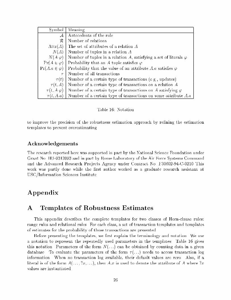
Before presenting the templates, we �rst explain the terminology and notation. We use

a notation to represent the repeatedly used parameters in the templates. Table 16 gives

this notation. Parameters of the form N(: : :) can be obtained by counting data in a given

database. To evaluate the parameters of the form � (: : :) needs to access transaction log

information. When no transaction log available, their default values are zero. Also, if a

literal is of the form A(: : : ; ?x; : : :), then A:x is used to denote the attribute of A where ?x

values are instantiated.

26

A.1 Range Rules

Consider a range rule of the form

�(?x)(=^

1�i�I

Ai ^^

1�j�J

Bj ^^

1�k�K

Lk;

where � is a predicate composed of a built-in predicate and constants (e.g., we can de�ne

�(?x) �?x � 100), Ai's are database literals where ?x occurs, and Lk's are built-in literals.

Three mutually exclusive classes of invalidating transactions and the templates to estimate

their probabilities are given as follows.

� T1: Update a tuple of Ai or Bj covered by the rule so that a new ?x value satis�es

the antecedent but does not satisfy �(?x).

Pr(T1) =X

1�i�I

u(Ai; Ai:x) +X

1�j�J

Xy2Attr(Bj)

u(Bj; y)

where for a relation A and one of its attribute A:z,

u(A;A:z) = u1 � u2 � u3 � u4 � u5;

u1 =� (update) + 1

� + 3

u2 =� (update; A) + 1

� (update) +R

u3 =� (update; AjA) + 1

� (update; A) + N(A)

N(AjA)

u4 =� (update; A:z) + 1

� (update; A) + jAttr(A)j

u5 = Pr(A:z 2 :�(?x) ^ A):

� T2: Insert a new tuple to a relation Ai or Bj so that the tuple satis�es all the an-

tecedents but not �(?x).

Pr(T2) =X

1�i�I

s(Ai) +X

1�j�J

s(Bj);

where for a relation A,

s(A) = s1 � s2 � s3;

s1 =� (insert) + 1

t+ 3

s2 =� (insert; A) + 1

� (insert) +R

s3 = Pr(A 2 :�(?x) ^ A):

27

� T3: Update one tuple of a relation Ai or Bj not covered by the rule so that the

resulting tuple satis�es all the antecedents but not �(?x).

Pr(T3) =X

1�i�I

Xw2Attr(Ai)�fA:xg

v(Ai; w) +X

1�j�J

Xy2Attr(Bj)

v(Bj ; y);

where for a relation A and its attribute A:z,

v(A;A:z) = v1 � v2 � v3 � v4 � v5;

v1 =� (update) + 1

� + 3

v2 =� (update; A) + 1

� (update) +R

v3 = 1�� (update; AjA ^ �(?x)) + 1

� (update; A) + N(A)

N(Aj�(?x)^A)

v4 =� (update; A:z) + 1

� (update; A) + jAttr(A)j

v5 = Pr(A:z 2 :�(?x)^ A):

A.2 Relational rules

Consider a relational rule of the form

C(?x)(=^

1�i�I

Ai ^^

1�j�J

Bj ^^

1�k�K

Lk;

where C(?x) is the abbreviation of C(: : : ; ?x; : : :) for a relation C in the database, Ai and

Bj 's are database literals, and Lk's are built-in literals. Five mutually exclusive classes

of invalidating transactions and the templates to estimate their probabilities are given as

follows.

� T1: Update an attribute of a tuple of Ai or Bj covered by the rule so that the new

value allows a new ?x value satis�es the antecedents but not the consequent.

Pr(T1) =X

1�i�I

u(Ai; Ai:x) +X

1�j�J

Xy2Attr(Bj)

u(Bj; y)

where for a relation A and one of its attribute A:z,

u(A;A:z) = u1 � u2 � u3 � u4 � u5;

u1 =� (update) + 1

� + 3

28

u2 =� (update; A) + 1

� (update) +R

u3 =� (update; AjA) + 1

� (update; A) + N(A)

N(AjA)

u4 =� (update; A:z) + 1

� (update; A) + jAttr(A)j

u5 = Pr(A:z 2 :C(?x) ^ A):

� T2: Insert a new tuple to Ai or Bj so that the new tuple allows a new ?x value satis�es

the antecedents but not the consequent.

Pr(T2) =X

1�i�I

s(Ai) +X

1�j�J

s(Bj);

where for a relation A,

s(A) = s1 � s2 � s3;

s1 =� (insert) + 1

t+ 3

s2 =� (insert; A) + 1

� (insert) +R

s3 = Pr(A 2 :C(?x) ^ A):

� T3: Update an attribute of a tuple of Ai or Bj not covered by the rule so that the

new value allows a new ?x value satis�es the antecedents but not the consequent.

Pr(T3) =X

1�i�I

Xw2Attr(Ai)�fA:xg

v(Ai; w) +X

1�j�J

Xy2Attr(Bj)

v(Bj ; y);

where for a relation A and its attribute A:z,

v(A;A:z) = v1 � v2 � v3 � v4 � v5;

v1 =� (update) + 1

� + 3

v2 =� (update; A) + 1

� (update) +R

v3 = 1�� (update; AjA ^ C(?x)) + 1

� (update; A) +N(A)

N(AjC(?x)^A)

v4 =� (update; A:z) + 1

� (update; A) + jAttr(A)j

v5 = Pr(A:z 2 :C(?x) ^ A):

29

� T4: Update C:x of all C tuples that share a certain C:x value that satis�es the

antecedents to a new value that does not satis�es the antecedents.

Pr(T4) =XX2Ix

p(X)N(CjC:x=X);

where Ix is the set of distinct values of C:x, and p(X) is the probability that the update

is applied to C tuples whose C:x = X. Pr(T4) can be approximated by

Pr(T4) � n2 � p(Y )n1;

where n1 is the minimal number of C tuples that is grouped by the same C:x value

denoted as Y , n2 is the number of all distinct C:x values, and

p(Y ) = p1 � p2 � p3 � p4 � p5;

where

p1 =� (update) + 1

� + 3

p2 =� (update; C) + 1

� (update) +R

p3 =� (update; CjC:x = Y ) + 1

� (update; C) + N(C)

N(CjC:x=Y )

p4 =� (update; C:x) + 1

� (update; C) + jAttr(C)j

p5 = Pr(C:x 2 :A):

� T5: Delete all C tuples that share a certain C:x value that satis�es the antecedents of

the rule.

Pr(T5) =XX2Ix

d(X)N(CjC:x=X);

where Ix is the set of distinct values of C:x, and d(X) is the probability that the

deletion is applied to C tuples whose C:x = X. Pr(T4) can be approximated by

Pr(T5) � n2 � d(Y )n1;

where n1 is the minimal number of C tuples that is grouped by the same C:x value

denoted as Y , n2 is the number of all distinct C:x values, and

d(Y ) = d1 � d2 � d3;

where

d1 =� (delete) + 1

� + 3

d2 =� (delete; C) + 1

� (delete) +R

d3 =� (delete; CjC:x = Y ) + 1

� (delete; C) + N(C)

N(CjC:x=Y )

:

30

References

[Agrawal et al., 1993] Rakesh Agrawal, Tomasz Imielinski, and Arun Swami. Database mining: A

performance perspective. IEEE Transactions on Knowledge and Data Engineering, 5(6):914{925,

December 1993.

[Ambite and Knoblock, 1995] Jose-Luis Ambite and Craig A. Knoblock. Reconciling distributed

information sources. InWorking Notes of the AAAI Spring Symposium on Information Gathering

in Distributed Heterogeneous Environments, Palo Alto, CA, 1995.

[Arens et al., 1993] Yigal Arens, Chin Y. Chee, Chun-Nan Hsu, and Craig A. Knoblock. Retrieving

and integrating data from multiple information sources. International Journal on Intelligent and

Cooperative Information Systems, 2(2):127{159, 1993.

[Arens et al., 1996] Yigal Arens, Craig A. Knoblock, and Wei-Min Shen. Query reformulation for

dynamic information integration. Journal of Intelligent Information Systems, Special Issue on

Intelligent Information Integration, 1996.

[Bacchus et al., 1992] Fahiem Bacchus, Adam Grove, Joseph Y. Halpern, and Daphne Koller.

From statistics to beliefs. In Proceedings of the Tenth National Conference on Arti�cial

Intelligence(AAAI-92), pages 602{608, San Jose, CA, 1992.

[Bacchus et al., 1993] Fahiem Bacchus, Adam Grove, Joseph Y. Halpern, and Daphne Koller. Sta-

tistical foundations for default reasoning. In Proceedings of the 13th International Joint Confer-

ence on Arti�cial Intelligence(IJCAI-93), pages 563{569, Chambery, France, 1993.

[Bacchus et al., 1994] Fahiem Bacchus, Adam Grove, Joseph Y. Halpern, and Daphne Koller.

Forming beliefs about a changing world. In Proceedings of the Twelfth National Conference

on Arti�cial Intelligence(AAAI-94), pages 222{229, Seattle, WA, 1994.

[Bacchus, 1988] Fahiem Bacchus. Representing and Reasoning with Probabilistic Knowledge. PhD

thesis, University of Alberta, Edmonton, Alta., Canada, 1988. Also available from MIT Press,

1990.

[Bell, 1995] Siegfried Bell. Discovery and maintenance of functional dependencies by independen-

cies. In Proceedings of the First International Conference on Knowledge Discovery and Data

Mining(KDD-95), Menlo Park, CA, 1995. AAAI Press.

[Cestnik and Bratko, 1991] Bojan Cestnik and Ivan Bratko. On estimating probabilities in tree

pruning. In Machine Learning { EWSL-91, European Working Session on Learning, pages 138{

150. Springer-Verlag, Berlin, Germany, 1991.

[Clark and Niblett, 1989] Peter Clark and Tim Niblett. The CN2 induction algorithm. Machine

Learning, 3(4):261{283, 1989.

31

[Cohen, 1993] William W. Cohen. E�cient pruning methods for separate-and-conquer rule

learning systems. In Proceedings of the 13th International Joint Conference on Arti�cial

Intelligence(IJCAI-93), Chambery, France, 1993.

[Cohen, 1995] William W. Cohen. Fast e�ective rule induction. In Machine Learning, Proceedings

of the 12th International Conference(ML-95), San Mateo, CA, 1995. Morgan Kaufmann.

[Cussens, 1993] James Cussens. Bayes and pesudo-Bayes estimates of conditional probabilities

and their reliability. In Machine Learning: ECML-93, pages 136{152, Berlin, Germany, 1993.

Springer-Verlag.

[Dao and Perry, 1995] Son Dao and Brad Perry. Applying a data miner to heterogeneous schema

integration. In Proceedings of the First International Conference on Knowledge Discovery and

Data Mining(KDD-95), Menlo Park, CA, 1995. AAAI Press.

[D�zeroski, 1996] Sa�so D�zeroski. Inductive logic programming and knowledge discovery in databases.

In Usama M. Fayyad, Gregory Piatetsky-Shapiro, Padhraic Smyth, and Ramasamy Uthurusamy,

editors, Advances in Knowledge Discovery and Data Mining, chapter 5. AAAI Press/MIT Press,

1996.

[Furnkranz and Widmer, 1994] Johannes Furnkranz and Gerhard Widmer. Incremental reduced

error prunning. In Machine Learning, Proceedings of the 11th International Conference(ML-94),

San Mateo, CA, 1994. Morgan Kaufmann.

[Ginsberg, 1987] Matthew L. Ginsberg. Readings in Nonmonotonic Reasoning. Morgan Kaufmann,

San Mateo, CA, 1987.

[Halpern, 1990] Joseph Y. Halpern. An analysis of �rst-order logics of probability. Arti�cial Intel-

ligence, 46(3), December 1990.

[Helmbold and Long, 1994] David P. Helmbold and Philip M. Long. Tracking drifting concepts by

minimizing disagreement. Machine Learning, 14:27{45, 1994.

[Howson and Urbach, 1988] Colin Howson and Peter Urbach. Scienti�c Reasoning: The Bayesian

Approach. Open Court, 1988.

[Hsu and Knoblock, 1993] Chun-Nan Hsu and Craig A. Knoblock. Reformulating query plans for

multidatabase systems. In Proceedings of the Second International Conference on Information

and Knowledge Management(CIKM-93), Washington, D.C., 1993.

[Hsu and Knoblock, 1994] Chun-Nan Hsu and Craig A. Knoblock. Rule induction for semantic

query optimization. In Machine Learning, Proceedings of the 11th International Conference(ML-

94), San Mateo, CA, 1994. Morgan Kaufmann.

32

[Hsu and Knoblock, 1996a] Chun-Nan Hsu and Craig A. Knoblock. Discovering robust knowledge

from dynamic closed-world data. In Proceedings of the Thirteenth National Conference on Arti-

�cial Intelligence (AAAI-96), Portland, Oregon, 1996. AAAI Press.

[Hsu and Knoblock, 1996b] Chun-Nan Hsu and Craig A. Knoblock. Using inductive learning to

generate rules for semantic query optimization. In Usama M. Fayyad, Gregory Piatetsky-Shapiro,

Padhraic Smyth, and Ramasamy Uthurusamy, editors, Advances in Knowledge Discovery and

Data Mining, chapter 17. AAAI Press/MIT Press, 1996.

[Hsu, 1996] Chun-Nan Hsu. Learning E�ective and Robust Knowledge for Semantic Query Op-

timization. PhD thesis, Department of Computer Science, University of Southern California,

1996.

[King, 1981] Jonathan J. King. Query Optimization by Semantic Reasoning. PhD thesis, Stanford

University, Department of Computer Science, 1981.

[Knoblock et al., 1994] Craig A. Knoblock, Yigal Arens, and Chun-Nan Hsu. Cooperating agents

for information retrieval. In Proceedings of the Second International Conference on Intelligent

and Cooperative Information Systems, Toronto, Ontario, Canada, 1994.

[Lavra�c and D�zeroski, 1994] Nada Lavra�c and Sa�so D�zeroski. Inductive Logic Programming: Tech-

niques and Applications. Ellis Horwood, 1994.

[Lloyd, 1987] John W. Lloyd. Foundations of Logic Programming. Springer-Verlag, Berlin, Ger-

many, 1987.

[Mannila and Raiha, 1994] Heikki Mannila and Kari-Jouko Raiha. Algorithms for inferring func-

tional dependencies from relations. Data and Knowledge Engineering, 12:83{99, 1994.

[Minton, 1988] Steven Minton. Learning E�ective Search Control Knowledge: An Explanation-

Based Approach. PhD thesis, Carnegie Mellon University, School of Computer Science, 1988.

[Pawlak, 1991] Zdzislaw Pawlak. Rough Sets: Theoretical aspects of Reasoning about Data. Kluwer,

Boston, MA, 1991.

[Piatetsky-Shapiro, 1984] Gregory Piatetsky-Shapiro. A Self-Organizing Database System { A Dif-

ferent Approach To Query Optimization. PhD thesis, Department of Computer Science, New

York University, 1984.

[Piatetsky-Shapiro, 1991] Gregory Piatetsky-Shapiro. Discovery, analysis, and presentation of

strong rules. In G. Piatetsky-Shapiro and William J. Frawley, editors, Knowledge Discovery

in Databases, pages 229{248. MIT Press, 1991.

33

[Raedt and Bruynooghe, 1993] Luc De Raedt and Maurice Bruynooghe. A theory of clausal discov-

ery. In Proceedings of the 13th International Joint Conference on Arti�cial Intelligence(IJCAI-

93), Chambery, France, 1993.

[Ramsay, 1988] Allan Ramsay. Formal Methods in Arti�cial Intelligence. Cambridge University

Press, Cambridge, U.K., 1988.

[Shafer and Pearl, 1990] Glenn Shafer and Judea Pearl. Readings in Uncertain Reasoning. Morgan

Kaufmann, San Mateo, CA, 1990.

[Shekhar et al., 1993] Shashi Shekhar, Babak Hamidzadeh, Ashim Kohli, and Mark Coyle. Learn-

ing transformation rules for semantic query optimization: A data-driven approach. IEEE Trans-

actions on Knowledge and Data Engineering, 5(6):950{964, 1993.

[Siegel et al., 1991] Michael D. Siegel, Edward Sciore, and Sharon Salveter. Rule discovery for

query optimization. In Gregory Piatetsky-Shapiro and William J. Frawley, editors, Knowledge

Discovery in Databases, pages 411{427. MIT Press, Cambridge, MA, 1991.

[Siegel, 1988] Michael D. Siegel. Automatic rule derivation for semantic query optimization. In

Larry Kerschberg, editor, Proceedings of the Second International Conference on Expert Database

Systems, pages 371{385. George Mason Foundation, Fairfax, VA, 1988.

[Sun and Yu, 1994] Wei Sun and Clement T. Yu. Semantic query optimization for tree and chain

queries. IEEE Trans. Knowledge and Data Engineering, 6(1):136{151, 1994.

[Ullman, 1988] Je�rey D. Ullman. Principles of Database and Knowledge-base Systems, volume

I,II. Computer Science Press, Palo Alto, CA, 1988.

[Widmer and Kubat, 1993] Gerhard Widmer and Miroslav Kubat. E�ective learning in dynamic

environments by explicit context tracking. In Machine Learning: ECML-93, Berlin, Germany,

1993. Springer-Verlag.

[Ziarko, 1995] Wojciech Ziarko. The special issue on rough sets and knowledge discovery. Compu-

tational Intelligence, 11(2), 1995.

34