Discontinuous Observers with strong convergence properties ...

Discontinuous Observers with strong convergenceproperties and some applications

Jaime A. [email protected]

Instituto de IngenierıaUniversidad Nacional Autonoma de Mexico

Mexico City, Mexico

Seminars in Systems and Control, CESAME, UCL, Belgium

24 April 2012

24 April 2012, Jaime A. Moreno Discontinuous Observers 1 / 59

Overview

1 Introduction

2 Observers a la Second Order Sliding Modes (SOSM)Super-Twisting ObserverGeneralized Super-Twisting Observers

3 Lyapunov Approach for Second-Order Sliding ModesGSTA without perturbations: ALEGSTA with perturbations: ARI

4 Optimality of the ST with noise

5 A Recursive Finite-Time Convergent Parameter Estimation AlgorithmThe Classical AlgorithmThe Proposed Algorithm

6 Conclusions


Overview

1 Introduction





6 Conclusions


Basic Observation Problem

Variations of the observation problem: with unknown inputs, practicalobservers, robust observers, stochastic framework to deal with noises, ....


An important Property: Observability

Consider a nonlinear system without inputs, x ∈ Rn, y ∈ R

x (t) = f (x (t)) , x (t0) = x0

y (t) = h (x (t))

Differentiating the output

y (t) = h (x (t))

y (t) =d

dth (x (t)) =

∂h (x)

∂xx (t) =

∂h (x)

∂xf (x) := Lf h (x)

y (t) =∂Lf h (x)

∂xx (t) =

∂Lf h (x)

∂xf (x) := L2

f h (x)

...

y (n−1) (t) =∂Ln−2

f h (x)

∂xx (t) =

∂Ln−2f h (x)

∂xf (x) := Ln−1

f h (x)

where Lkf h (x) are Lie’s derivatives of h along f .


Evaluating at t = 0y (0)y (0)y (0)...

y (k) (0)

=

h (x0)Lf h (x0)L2f h (x0)

...Lkf h (x0)

:= On (x0)

On (x): Observability map

Theorem

If On (x) is injective (invertible) → The NL system is observable.


Observability Form

In the coordinates of the output and its derivatives

z = On (x) , x = O−1n (z)

the system takes the (observability) form

z1 = z2

z2 = z3...

zn = φ (z1, z2, . . . , zn)y = z1

So we can consider a system in this form as a basic structure.


A Simple Observer and its Properties

Plant: x1 = x2 , x2 = w(t)Observer: ˙x1 = −l1 (x1 − x1) + x2 , ˙x2 = −l2 (x1 − x1)Estimation Error: e1 = x1 − x1, e2 = x2 − x2

e1 = −l1e1 + e2 , e2 = −l2e1 − w (t)

Figure: Linear Plant with an unknown input and a Linear Observer.


0 20 40 600

10

20

30

40

50

60

Time (sec)

Sta

te x

10 20 40 60

0

0.5

1

1.5

2

Time (sec)

Sta

tet

x2

0 20 40 60−1

0

1

2

3

4

Time (sec)

Estim

atio

n e

rro

r e

1

0 20 40 60−1.5

−1

−0.5

0

0.5

1

1.5

2

Time (sec)

Estim

atio

n e

rro

r e

2

Linear Observer Linear Observer

Figure: Behavior of Plant and the Linear Observer without unknown input.


0 20 40 600

20

40

60

80

100

120

140

Time (sec)

Sta

te x

10 20 40 60

0.5

1

1.5

2

2.5

3

3.5

4

Time (sec)

Sta

tet

x2

0 20 40 60−2

−1

0

1

2

3

4

Time (sec)

Estim

atio

n e

rro

r e

1

0 20 40 60−1.5

−1

−0.5

0

0.5

1

1.5

2

Time (sec)

Estim

atio

n e

rro

r e

2


Figure: Behavior of Plant and the Linear Observer with unknown input.


0 20 40 600

10

20

30

40

50

60

Time (sec)S

tate

x1

0 20 40 600

0.5

1

1.5

2

Time (sec)

Sta

tet

x2

0 20 40 60−1

0

1

2

3

4

Time (sec)

Estim

atio

n e

rro

r e

1

0 20 40 60−1.5

−1

−0.5

0

0.5

1

1.5

2

Time (sec)

Estim

atio

n e

rro

r e

2


Figure: Behavior of Plant and the Linear Observer without UI with large initialconditions.


0 20 40 600

10

20

30

40

50

60

Time (sec)S

tate

x1

0 20 40 600

0.5

1

1.5

2

Time (sec)

Sta

tet

x2

0 20 40 60−1

0

1

2

3

4

Time (sec)

Estim

atio

n e

rro

r e

1

0 20 40 60−1.5

−1

−0.5

0

0.5

1

1.5

2

Time (sec)

Estim

atio

n e

rro

r e

2


Figure: Behavior of Plant and the Linear Observer without UI with very largeinitial conditions.


Recapitulation.

Linear Observer for Linear Plant

If no unknown inputs/Uncertainties: it converges exponentially fast.

If there are unknown inputs/Uncertainties: no convergence. At bestbounded error.

Convergence time depends on the initial conditions of the observer

Is it possible to alleviate these drawbacks?


Recapitulation.







Recapitulation.







Recapitulation.







Recalling Sliding Mode Control

Consider a plant

σ = α + u, σ(0) = 1

where α ∈ (−1, 1) is a perturbation.Continuous (linear) Control

σ = α− kσ, k > 0, σ(0) = 1

Comments:

RHS of DE continuous (linear).

If α = 0 exponential (asymptotic) convergence to σ = 0.

If α 6= 0 practical convergence.


Discontinuous Control

σ = α− sign(σ), σ(0) = 1

with α ∈ (−1, 1).

σ > 0⇒ σ =< 0

σ < 0⇒ σ => 0

y σ(t) ≡ 0, ∀t ≥ T .

Comments:

¿0 = α− sign(0)?

RHS of DE isdiscontinuous.

After arriving at σ = 0,sliding on σ ≡ 0.

0 0.5 1 1.5 2 2.5 3 3.5 4 4.5 5

0

0.5

1

0 0.5 1 1.5 2 2.5 3 3.5 4 4.5 5

−1

−0.5

0

0.5

1

0 0.5 1 1.5 2 2.5 3 3.5 4 4.5 5

0.4

0.6

0.8

1

1.2

σ

u

u

Finite-Time convergence.

Differential Inclusion.

σ ∈ [−α, α]− sign(σ)


Why sliding-mode (discontinuous) control?

Precise.

More than robust (insensitive) against a class of perturbations.

When to use sliding-mode control?

Unaccounted dynamics.

Parametric uncertainty.

Severe external perturbations.

Some applications

Robotics.

Aerospace vehicles.

Electric systems (motors, generators, etc).

Automobiles.

Biomedical.

etc.


Sliding Mode Observer (SMO)

Figure: Linear Plant with an unknown input and a SM Observer.24 April 2012, Jaime A. Moreno Discontinuous Observers 15 / 59

0 20 40 600

10

20

30

40

50

60

Time (sec)

Sta

te x

10 20 40 60

0

0.5

1

1.5

2

Time (sec)

Sta

tet

x2

0 20 40 60−1

0

1

2

3

4

Time (sec)

Estim

atio

n e

rro

r e

1

0 20 40 60−1.5

−1

−0.5

0

0.5

1

1.5

2

Time (sec)

Estim

atio

n e

rro

r e

2

Linear Observer

Nonlinear ObserverLinear Observer

Nonlinear Observer

Figure: Behavior of Plant and the SM Observer without unknown input.


0 20 40 600

20

40

60

80

100

120

140

Time (sec)

Sta

te x

10 20 40 60

0.5

1

1.5

2

2.5

3

3.5

4

Time (sec)

Sta

tet

x2

0 20 40 60−1

0

1

2

3

4

Time (sec)

Estim

atio

n e

rro

r e

1

0 20 40 60−1.5

−1

−0.5

0

0.5

1

1.5

2

Time (sec)

Estim

atio

n e

rro

r e

2

Linear Observer

Nonlinear ObserverLinear Observer

Nonlinear Observer

Figure: Behavior of Plant and the SM Observer with unknown input.


Recapitulation.

Sliding Mode Observer for Linear Plant

If no unknown inputs/Uncertainties: e1 converges in finite time, ande2 converges exponentially fast.

If there are unknown inputs/Uncertainties: no convergence. At bestbounded error. Only e1 converges in finite time!


It is not the solution we expected! None of the objectives has beenachieved!


Recapitulation.







Recapitulation.







Recapitulation.







Overview

1 Introduction





6 Conclusions


Overview

1 Introduction





6 Conclusions


Super-Twisting Algorithm (STA)

Plant:x1 = x2 ,x2 = w(t)

Observer:˙x1 = −l1 |e1|

12 sign (e1) + x2 ,

˙x2 = −l2 sign (e1)

Estimation Error: e1 = x1 − x1, e2 = x2 − x2

e1 = −l1 |e1|12 sign (e1) + e2

e2 = −l2 sign (e1)− w (t) ,

Solutions in the sense of Filippov.


Figure: Linear Plant with an unknown input and a SOSM Observer.


0 20 40 600

10

20

30

40

50

60

Time (sec)

Sta

te x

10 20 40 60

0

0.5

1

1.5

2

Time (sec)

Sta

tet

x2

0 20 40 60−1

0

1

2

3

4

Time (sec)

Estim

atio

n e

rro

r e

1

0 20 40 60−1.5

−1

−0.5

0

0.5

1

1.5

2

Time (sec)

Estim

atio

n e

rro

r e

2

Linear Observer

Nonlinear Observer

Linear Observer

Nonlinear Observer

Figure: Behavior of Plant and the Non Linear Observer without unknown input.


0 20 40 600

20

40

60

80

100

120

140

Time (sec)

Sta

te x

10 20 40 60

0.5

1

1.5

2

2.5

3

3.5

4

Time (sec)

Sta

tet

x2

0 20 40 60−1

0

1

2

3

4

Time (sec)

Estim

atio

n e

rro

r e

1

0 20 40 60−1.5

−1

−0.5

0

0.5

1

1.5

2

Time (sec)

Estim

atio

n e

rro

r e

2

Linear Observer

Nonlinear Observer

Linear Observer

Nonlinear Observer

Figure: Behavior of Plant and the Non Linear Observer with unknown input.


0 20 40 600

10

20

30

40

50

60

Time (sec)S

tate

x1

0 20 40 600

0.5

1

1.5

2

Time (sec)

Sta

tet

x2

0 20 40 60−1

0

1

2

3

4

Time (sec)

Estim

atio

n e

rro

r e

1

0 20 40 60−1.5

−1

−0.5

0

0.5

1

1.5

2

Time (sec)

Estim

atio

n e

rro

r e

2

Linear Observer

Nonlinear Observer

Linear Observer

Nonlinear Observer

Figure: Behavior of Plant and the Non Linear Observer without UI with largeinitial conditions.


Recapitulation.

Super-Twisting Observer for Linear Plant

If no unknown inputs/Uncertainties: e1 and e2 converge in finite-time!

If there are unknown inputs/Uncertainties: e1 and e2 converge infinite-time! Observer is insensitive to perturbation/uncertainty!

Convergence time depends on the initial conditions of the observer.This objective is not achieved!


Recapitulation.






Recapitulation.






Overview

1 Introduction





6 Conclusions


Generalized Super-Twisting Algorithm (GSTA)

Plant:x1 = x2 ,x2 = w(t)

Observer:˙x1 = −l1φ1 (e1) + x2 ,˙x2 = −l2φ2 (e1)

Estimation Error: e1 = x1 − x1, e2 = x2 − x2

e1 = −l1φ1 (e1) + e2

e2 = −l2φ2 (e1)− w (t) ,


φ1 (e1) = µ1 |e1|12 sign (e1) + µ2 |e1|

32 sign (e1) , µ1 , µ2 ≥ 0 ,

φ2 (e1) =µ2

1

2sign (e1) + 2µ1µ2e1 +

3

2µ2

2 |e1|2 sign (e1) ,


Figure: Linear Plant with an unknown input and a Non Linear Observer.


0 20 40 600

10

20

30

40

50

60

Time (sec)S

tate

x1

0 20 40 600

0.5

1

1.5

2

Time (sec)

Sta

tet

x2

0 20 40 60−1

0

1

2

3

4

Time (sec)

Estim

atio

n e

rro

r e

1

0 20 40 60−1.5

−1

−0.5

0

0.5

1

1.5

2

Time (sec)

Estim

atio

n e

rro

r e

2

Linear Observer

Nonlinear Observer

Linear Observer

Nonlinear Observer

Figure: Behavior of Plant and the Non Linear Observer without unknown inputand large initial conditions.


0 20 40 600

10

20

30

40

50

60

Time (sec)S

tate

x1

0 20 40 600

0.5

1

1.5

2

Time (sec)

Sta

tet

x2

0 20 40 60−1

0

1

2

3

4

Time (sec)

Estim

atio

n e

rro

r e

1

0 20 40 60−1.5

−1

−0.5

0

0.5

1

1.5

2

Time (sec)

Estim

atio

n e

rro

r e

2

Linear Observer

Nonlinear Observer

Linear Observer

Nonlinear Observer

Figure: Behavior of Plant and the Non Linear Observer without unknown inputand very large initial conditions.


0 20 40 600

20

40

60

80

100

120

140

Time (sec)

Sta

te x

10 20 40 60

0.5

1

1.5

2

2.5

3

3.5

4

Time (sec)

Sta

tet

x2

0 20 40 60−1

0

1

2

3

4

Time (sec)

Estim

atio

n e

rro

r e

1

0 20 40 60−1.5

−1

−0.5

0

0.5

1

1.5

2

Time (sec)

Estim

atio

n e

rro

r e

2

Linear Observer

Nonlinear Observer

Linear Observer

Nonlinear Observer

Figure: Behavior of Plant and the Non Linear Observer with UI with large initialconditions.


Effect: Convergence time independent of I.C.

101

102

103

104

0

2

4

6

8

10

12

14

16

norm of the initial condition ||x(0)|| (logaritmic scale)

Co

nve

rge

nce

Tim

e T

NSOSMO

GSTA with linear term

STO

Figure: Convergence time when the initial condition grows.


Recapitulation.

Generalized Super-Twisting Observer for Linear Plant



Convergence time is independent of the initial conditions of theobserver!.

All objectives were achieved!

How to proof these properties?


Recapitulation.








Recapitulation.








Recapitulation.








Recapitulation.








What have we achieved?

An algorithm

Robust: it converges despite of unknown inputs/uncertainties

Exact: it converges in finite-time

The convergence time can be preassigned for any arbitrary initialcondition.

But there is no free lunch!

It is useful for

Observation

Estimation of perturbations/uncertainties

Control: Nonlinear PI-Control

in practice?

Some Generalizations are available but Still a lot is missing


Overview

1 Introduction





6 Conclusions


Lyapunov functions:

1 We propose a Family of strong Lyapunov functions, that areQuadratic-like

2 This family allows the estimation of convergence time,

3 It allows to study the robustness of the algorithm to different kinds ofperturbations,

4 All results are obtained in a Linear-Like framework, known fromclassical control,

5 The analysis can be obtained in the same manner for a linearalgorithm, the classical ST algorithm and a combination of bothalgorithms (GSTA), that is non homogeneous.


Overview

1 Introduction





6 Conclusions


Generalized STA

x1 = −k1φ1 (x1) + x2

x2 = −k2φ2 (x1) ,(1)


φ1 (e1) = µ1 |e1|12 sign (e1) + µ2 |e1|q sign (e1) , µ1 , µ2 ≥ 0 , q ≥ 1 ,

φ2 (e1) =µ2

1

2sign (e1) +

(q +

1

2

)µ1µ2 |e1|q−

12 sign (e1) +

+ qµ22 |e1|2q−1 sign (e1) ,

Standard STA: µ1 = 1, µ2 = 0

Linear Algorithm: µ1 = 0, µ2 > 0, q = 1.

GSTA: µ1 = 1, µ2 > 0, q > 1.


Quadratic-like Lyapunov Functions

System can be written as:

ζ = φ′1 (x1)Aζ , ζ =

[φ1 (x1)

x2

], A =

[−k1 1−k2 0

].

Family of strong Lyapunov Functions:

V (x) = ζTPζ , P = PT > 0 .

Time derivative of Lyapunov Function:

V (x) = φ′1 (x1) ζT(

ATP + PA)

ζ = −φ′1 (x1) ζTQζ

Algebraic Lyapunov Equation (ALE):

ATP + PA = −Q


Figure: The Lyapunov function.


Lyapunov Function

Proposition

If A Hurwitz then x = 0 Finite-Time stable (if µ1 = 1) and for everyQ = QT > 0, V (x) = ζTPζ is a global, strong Lyapunov function,with P = PT > 0 solution of the ALE, and

V ≤ −γ1 (Q, µ1)V12 (x)− γ2 (Q, µ2)V (x) ,

where

γ1 (Q, µ1) , µ1λmin {Q} λ

12min{P}

2λmax {P}, γ2 (Q, µ2) , µ2

λmin {Q}λmax {P}

If A is not Hurwitz then x = 0 unstable.


Convergence Time

Proposition

If k1 > 0 , k2 > 0, and µ2 ≥ 0 a trajectory of the GSTA starting atx0 ∈ R2 converges to the origin in finite time if µ1 = 1, and it reachesthat point at most after a time

T =

2

γ1(Q,µ1)V

12 (x0) if µ2 = 0

2γ2(Q,µ2)

ln(

γ2(Q,µ2)γ1(Q,µ1)

V12 (x0) + 1

)if µ2 > 0

,

When µ1 = 0 the convergence is exponential.

For Design: T depends on the gains!


Overview

1 Introduction





6 Conclusions


GSTA with perturbations: ARI

GSTA with time-varying and/or nonlinear perturbations

x1 = −k1φ1 (x1) + x2

x2 = −k2φ2 (x1) + ρ (t, x) .

Assume2 |ρ (t, x)| ≤ δ

Analysis: The construction of Robust Lyapunov Functions can be donewith the classical method of solving an Algebraic Ricatti Inequality (ARI),or equivalently, solving the LMI[

ATP + PA + εP + δ2CTC PBBTP −1

]≤ 0 ,

where

A =

[−k1 1−k2 0

], C =

[1 0

], B =

[01

].


Overview

1 Introduction





6 Conclusions


Derivation of a signal under noise

Signal model: x1 := σ and x2 := σ

x1(t) = x2(t),x2(t) = ρ(t) = −σ(t),y(t) = x1(t) + η(t),

where|ρ(t)| ≤ L, |η(t)| ≤ δ, ∀t ≥ 0.

The estimator (differentiator/observer) proposed is:

˙x1 = − α1ε φ1(x1 − y) + x2,

˙x2 = − α2ε2 φ2(x1 − y),

where

φ1(x) = µ1|x |12 sign(x) + µ2x , µ1, µ2 ≥ 0

φ2(x) =12 µ2

1sign(x) + 32 µ1µ2|x |

12 sign(x) + µ2

2x ,


Derivation of a signal under noise

Signal model: x1 := σ and x2 := σ

x1(t) = x2(t),x2(t) = ρ(t) = −σ(t),y(t) = x1(t) + η(t),

where|ρ(t)| ≤ L, |η(t)| ≤ δ, ∀t ≥ 0.

The estimator (differentiator/observer) proposed is:

˙x1 = − α1ε φ1(x1 − y) + x2,

˙x2 = − α2ε2 φ2(x1 − y),

where

φ1(x) = µ1|x |12 sign(x) + µ2x , µ1, µ2 ≥ 0

φ2(x) =12 µ2

1sign(x) + 32 µ1µ2|x |

12 sign(x) + µ2

2x ,


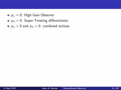
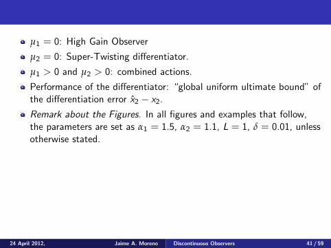
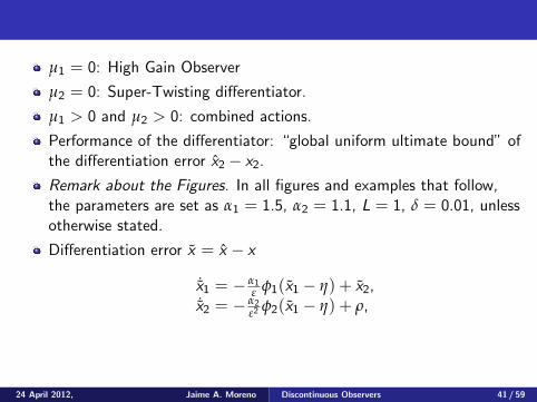
µ1 = 0: High Gain Observer

µ2 = 0: Super-Twisting differentiator.

µ1 > 0 and µ2 > 0: combined actions.

Performance of the differentiator: “global uniform ultimate bound” ofthe differentiation error x2 − x2.

Remark about the Figures. In all figures and examples that follow,the parameters are set as α1 = 1.5, α2 = 1.1, L = 1, δ = 0.01, unlessotherwise stated.

Differentiation error x = x − x

˙x1 = − α1ε φ1(x1 − η) + x2,

˙x2 = − α2ε2 φ2(x1 − η) + ρ,








˙x1 = − α1ε φ1(x1 − η) + x2,

˙x2 = − α2ε2 φ2(x1 − η) + ρ,








˙x1 = − α1ε φ1(x1 − η) + x2,

˙x2 = − α2ε2 φ2(x1 − η) + ρ,








˙x1 = − α1ε φ1(x1 − η) + x2,

˙x2 = − α2ε2 φ2(x1 − η) + ρ,








˙x1 = − α1ε φ1(x1 − η) + x2,

˙x2 = − α2ε2 φ2(x1 − η) + ρ,








˙x1 = − α1ε φ1(x1 − η) + x2,

˙x2 = − α2ε2 φ2(x1 − η) + ρ,


The performance of linear and ST differentiators.

0 0.1 0.2 0.3 0.4 0.5 0.6 0.7 0.8 0.90

0.1

0.2

0.3

0.4

0.5

0.6

gain ε

diffe

ren

tia

tio

n e

rro

r

0 0.5 1 1.5 2 2.5 3 3.5 40

1

2

3

4

5

6

7

gain ε

diffe

rentiation e

rror

0 1 2 3 4 5 6 7 80

0.5

1

1.5

2

2.5

3

gain ε

diffe

rentiation e

rror

Figure: Ultimate bound of the differentiation error as a function of ε. Solid: linearcase µ1 = 0, µ2 = 1; dashed: pure ST case µ1 = 1, µ2 = 0. Left: parametersL = 1, δ = 0.01; middle: parameters L = 1, δ = 1; right: parametersL = 0.1, δ = 1.


0 1 2 3 4 5 6 7 80

0.1

0.2

0.3

0.4

0.5

0.6

gain ε

steady

state

err

or

0 0.2 0.4 0.6 0.8 1 1.2 1.4 1.6 1.8 20

0.1

0.2

0.3

0.4

0.5

0.6

0.7

0.8

0.9

1

gain ε

ste

ad

y st

ate

err

or

Figure: Steady state error in the differentiation versus the gain fromL = 1, δ = 0.01 to L = 0.001, δ = 0.01. The figure on the right is a zoom of theleft figure. Solid: linear case µ1 = 0, µ2 = 1; dashed: pure ST caseµ1 = 1, µ2 = 0.


Advantages of the GST

0 0.1 0.2 0.3 0.4 0.5 0.6 0.70.3

0.4

0.5

0.6

0.7

0.8

0.9

gain ε

diffe

ren

tia

tio

n e

rro

r

Figure: Ultimate bound of the differentiation error as a function of ε, for L = 1and δ = 0.01. Solid: linear case µ1 = 0, µ2 = 1; dashed: pure ST caseµ1 = 1, µ2 = 0; dotted: two experiments µ1 = 0.8, µ2 = 0.2 andµ1 = 0.5, µ2 = 0.5 (with circles).24 April 2012, Jaime A. Moreno Discontinuous Observers 44 / 59

The sensitivity to variations in the noise amplitude

0 0.01 0.02 0.03 0.04 0.05 0.06 0.07 0.08 0.09 0.10

0.5

1

1.5

2

2.5

noise amplitude δ

diffe

rentiation e

rror

0 0.01 0.02 0.03 0.04 0.05 0.06 0.07 0.08 0.09 0.10

0.5

1

1.5

noise amplitude δ

diffe

rentiation e

rror

Figure: The differentiation error as a function of the noise amplitude. Solid:linear case µ1 = 0, µ2 = 1; dashed: pure ST case µ1 = 1, µ2 = 0; dotted: GSTcase with µ1 = µ2 = 0.5. Dash-dot: the nominal noise 0.01 for which theoptimal gains are selected. Left: for L = 1, Right: for L = 0.


Sensitivity to variations in the perturbation amplitude.

0 0.2 0.4 0.6 0.8 1 1.2 1.4 1.6 1.8 2

0

0.1

0.2

0.3

0.4

0.5

0.6

0.7

0.8

perturbation amplitude L

diffe

rentiation e

rror

Figure: The differentiation error as a function of the perturbation amplitude, forδ = 0.01. Solid: linear µ1 = 0, µ2 = 1; dashed: ST µ1 = 1, µ2 = 0; dotted: GSTµ1 = µ2 = 0.5. Dash-dotted: the nominal perturbation L = 1 for which theoptimal gains are selected.24 April 2012, Jaime A. Moreno Discontinuous Observers 46 / 59

0 5 10 15 20 25 30 35 40 45 501

1.5

2

2.5

3

3.5

4

4.5

5

Time (sec)

Sta

tet x

2

0 5 10 15 20 25 30 35 40 45 50−0.5

−0.4

−0.3

−0.2

−0.1

0

0.1

0.2

0.3

0.4

0.5

Time (sec)E

stim

ation e

rror

e2

Linear Observer

Nonlinear Observer

Figure: Behavior of Linear and ST Observers under noise and perturbation.


Overview

1 Introduction





6 Conclusions


Background

Super Twisting-Algorithm

Applications: Differentiator [Levant, 1998], [Levant, 2003], Controller[Levant, 2003], Observer [Davila et al., 2005] and as an observer andparameter estimator [Davila et al., 2006].

[Moreno, 2009], (Generalized Super-Twisting Algorithm).

Adaptive Systems

Some documents that summarize several techniques are[Narendra and Annaswamy, 1989], [Sastry and Bodson, 1989],[Ioannou and Sun, 1996] and [Ioannou and Findan, 2006] among others.

Finite-Time Parameter Estimation

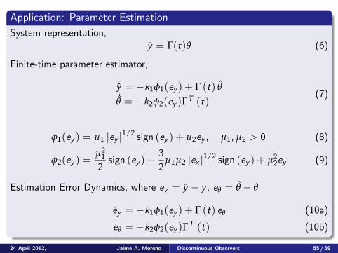
Finite-Time Parameter Estimator ([Adetola and Guay, 2008])


Overview

1 Introduction





6 Conclusions


[Morgan and Narendra, 1977]

x1 = A(t)x1 + B(t)x2

x2 = −BT (t)P(t)x1(2)

where xi ∈ Rni , i = 1, 2, A(t), B(t) are matrices of bounded piecewisecontinuous functions.

There exist a symmetric, positive definite matrix P(t), which satisfies

P(t) + AT (t)P(t) + P(t)A(t) = −Q(t)

Persistence of Excitation Conditions: B(t) is smooth,∣∣B(t)

∣∣ isuniformly bounded, there exist T > 0, ε > 0 such that for any unitvector w ∈ Rn2 ∫ t+T

t‖B(τ)w‖ dτ ≥ ε (3)

Then x(t)→ 0 exponentially.


Application: Parameter Estimation

Linearly parametrized System

y = α(x , t) + Γ(t)θ

Parameter Estimation Algorithm

˙y = α(x , t) + Γ(t)θ − kyey˙θ = −kθΓT (t)ey

Defining errors as ey = y − y and eθ = θ − θ.Error Dynamics

ey = −kyey + Γ(t)eθ˙θ = −kθΓT (t)ey


Overview

1 Introduction





6 Conclusions


x1 = A(t)φ1(x1) + B(t)x2

x2 = −BT (t)P(t)φ2(x1)+δ (t)(4)

where

φ1(x1) = µ1 |x1|1/2 sign (x1) + µ2x1, µ1, µ2 > 0

φ2(x1) =µ2

12 sign (x1) +

23 µ1µ2 |x1|1/2 sign (x1) + µ2

2x1

where x1 ∈ Rn1 , x2 ∈ Rn2 , n1 = 1, n2 ≥ 1, µ1 > 0 y µ2 ≥ 0

There exist a symmetric, positive definite matrix P(t), which satisfies

P(t) + AT (t)P(t) + P(t)A(t) = −Q(t)

Persistence of Excitation Conditions (PE): There exist T0, ε0, δ0,with t2 ∈ [t, t + T ] such that for any unit vector w ∈ Rn2∥∥∥∥ 1

T0

∫ t2+δ0

t2

B(τ)w dτ

∥∥∥∥ ≥ ε0 (5)


Finite-Time Convergence

Under PE conditions, if δ(t) = 0 then x(t)→ 0 in Finite-Time.

Robustness

Under PE conditions, if δ(t) is bounded then x(t) is bounded (ISS).Under some extra conditions it converges in finite time.


Case (µ1, µ2, p, q)

Linear (0,1,–,1)

STA (1,0,1/2,–)

GSTA (1,1,1/2,q)


Idea of the Proof

Under PE conditions it is possible to construct a strict Lyapunov function[Moreno, 2009]

V (t, x) = ζT Π(t)ζ

ζT =[ζ1 ζT2

]=[φ1(x1) xT

2

]V ≤ −γ1V 1/2 − γ2V


Application: Parameter Estimation

System representation,y = Γ(t)θ (6)

Finite-time parameter estimator,

˙y = −k1φ1(ey ) + Γ (t) θ˙θ = −k2φ2(ey )ΓT (t)

(7)

φ1(ey ) = µ1 |ey |1/2 sign (ey ) + µ2ey , µ1, µ2 > 0 (8)

φ2(ey ) =µ2

1

2sign (ey ) +

3

2µ1µ2 |ex |1/2 sign (ey ) + µ2

2ey (9)

Estimation Error Dynamics, where ey = y − y , eθ = θ − θ

ey = −k1φ1(ey ) + Γ (t) eθ (10a)

eθ = −k2φ2(ey )ΓT (t) (10b)


Example: A simple pendulum

x1 = x2 (11a)

x2 =1

Ju − Mgl

2Jsin x1 −

Vs

Jx2 (11b)

x1 angular position, x2 angular velocity, M mass, g gravity, L rope’slength mass and J = ML2 mass inertia.Parameter’s estimator

˙x2 = −k1φ1(ex2) + Γθ (12a)

˙θ = −k2φ2(ex2)ΓT (12b)

ex2 = x2 − x2 velocity’s error, Γ =[x2 sin x1 u

]regressor,

θ =[− Vs

J− Mg L

J1J

]vector of unknown parameters, φ1(·) and φ2(·)

are given as in the GSTA.24 April 2012, Jaime A. Moreno Discontinuous Observers 56 / 59

Parameter’s estimation

0 10 20 30 40 50−2.5

−2

−1.5

−1

−0.5

0

0.5

Time (sec)θ 1

andθ 1

θ1

θ1 with linear algorithm

θ1 with nonlinear algorithm

0 10 20 30 40 50−12

−10

−8

−6

−4

−2

0

Time (sec)

θ 2an

dθ 2

θ2θ2 with linear algorithmθ2 with nonlinear algorithm

0 10 20 30 40 50−1

−0.5

0

0.5

1

1.5

2

2.5

Time (sec)

θ 3an

dθ 3

θ3



Figure: Parameter estimation of θ1, θ2 and θ3 with GSTA and with linearalgorithm.


Parameter’s estimation, with perturbation in θ1 = −0.2 + 0.2sin(t)

0 10 20 30 40 50−2

−1.5

−1

−0.5

0

0.5

Time (sec)θ 1

andθ 1

θ1



0 10 20 30 40 50−12

−10

−8

−6

−4

−2

0

2

Time (sec)

θ 2an

dθ 2

θ2θ2 with linear algorithmθ2 with nonlinear algorithm

0 10 20 30 40 50−1

−0.5

0

0.5

1

1.5

2

Time (sec)

θ 3an

dθ 3

θ3



Figure: Parameter estimation of θ1, θ2 and θ3 with GSTA and with linearalgorithm.


Overview

1 Introduction





6 Conclusions


Conclusions

1 The GSTO is an observer that isRobust: it converges despite of unknown inputs/uncertaintiesExact: it converges in finite-timePreassigned Convergence time for any initial condition.But there is no free lunch!

2 It can be extended to estimate parameters in finite time withapplications in Adaptive Control

3 Applications for Bioreactors seem to be attractive due to:Robustness against uncertaintiesPossibility of reconstructing uncertainties, e.g. reaction rates

4 Lyapunov functions for Higher Order algorithms is an ongoing work.

5 Useful for control, reaction rate parameters (functional form)estimation, ...


Thank you!


Overview

7 Some ApplicationsFinite-Time, robust MRAC


Overview

7 Some ApplicationsFinite-Time, robust MRAC


Introduction

Direct Model Reference Adaptive Control (MRAC) is a well-knownapproach for adaptive control of linear and some nonlinear systems.

If Plant has relative degree n∗ = 1 and the reference model is StrictlyPositive Real (SPR), the controller is particularly simple toimplement, and to design.

The Adjustment Mechanism of the MRAC is basically a parameterestimation algorithm.

Our objective: Modify the Adjustment Mechanism of the classicalDirect MRAC by adding the Super-Twisting-Like nonlinearities, so asto achieve the finite-time convergence and robustness properties.


Introduction






Introduction






Introduction






MRAC with relative degree n∗ = 1

Figure: General structure of MRAC scheme.


SISO Plant: yp = Gp(s)up = kpZp(s)Rp(s)

, Relative degree n∗ = 1.

Reference model: ym = Wm(s)r = kmZm(s)Rm(s)

Hypothesis:

A1 An upper bound n of the degree np of Rp(s) is known.A2 The relative degree n∗ = np −mp of Gp(s) is one, i.e.

n∗ = 1.A3 Zp(s) is a monic Hurwitz polynomial of degree

mp = np − 1.A4 The sign of the high frequency gain kp is known.B1 Zm(s), Rm(s) are monic Hurwitz polynomials of degree

qm, pm, respectively, where pm ≤ n.B2 The relative degree n∗m = pm − qm of Wm is the same

as that of Gp(s), i.e., n∗m = n∗ = 1.B3 Wm(s) is designed to be Strictly Positive Real (SPR).


Solution of the MRC problem for known parameters:

w1 = Fw1 + gup, w1(0) = 0 (13a)

w2 = Fw2 + gyp, w2(0) = 0 (13b)

up = θ∗Tw (13c)

w =[wT

1 wT2 yp r

]T, θ∗ =

[θ∗T1 θ∗T2 θ∗T3 c∗0

]T(14)

For unknown parameters the control law is

up = θT (t)w (15)

θ (t) = −Γe1w sign (ρ∗) , (16)

e1 = yp − ym , sign (ρ∗) = sign

(kpkm

), Γ = ΓT > 0 . (17)


Classical MRAC

Theorem

The MRAC scheme guarantees that:

1 All signals in the closed-loop plant are bounded and the tracking errore1 converges to zero asymptotically for any reference input r ∈ L∞ .

2 If r is sufficiently rich of order 2n, r ∈ L∞ and Zp(s), Rp(s) arerelatively coprime, then the parameter error |θ| = |θ − θ∗| and thetracking error e1 converge to zero exponentially fast.


Modified MRAC

Modified adaptive control law

up =θT (t)w − k1φ1 (e1) sign (ρ∗)

θ (t) =− Γφ2 (e1)w sign (ρ∗) ,

φ1 (e1) = µ1 |e1|1/2 sign (e1) + µ2e1

φ2 (e1) =µ2

12 sign (e1) +

32 µ1µ2 |e1|1/2 sign (e1) + µ2

2e1

(18)

and µ1 > 0, µ2 > 0.


Theorem

The modified MRAC scheme guarantees that:

1 All signals in the closed-loop plant are bounded and the tracking errore1 converges to zero asymptotically for any reference input r ∈ L∞ .

2 If r is sufficiently rich of order 2n, r ∈ L∞ and Zp(s), Rp(s) arerelatively coprime, then the parameter error |θ| = |θ − θ∗| and thetracking error e1 converge to zero in finite time.

3 If PE is satisfied then algorithm is robust (ISS)


Example

Second order plant yp = (s+1)s2−3s+1

up .

Reference model ym = 1s+1 r .

Nominal controller

w1 = −2w1 + up, w1(0) = 0w2 = −2w2 + yp, w2(0) = 0up = θ1w1 + θ2w2 + θ3yp + c0r ,

(19)

θ =[θ1 θ2 θ3 c0

]T, w =

[w1 w2 yp r

]T, and

Nominal parameter values:

θ∗ =[θ∗1 θ∗2 θ∗3 c∗0

]T=[0 , 6 , −5 , 1

]T.

Three simulation scenarios will be presented.


Example


up .


Nominal controller


(19)

θ =[θ1 θ2 θ3 c0

]T, w =

[w1 w2 yp r

]T, and


θ∗ =[θ∗1 θ∗2 θ∗3 c∗0

]T=[0 , 6 , −5 , 1

]T.



Example


up .


Nominal controller


(19)

θ =[θ1 θ2 θ3 c0

]T, w =

[w1 w2 yp r

]T, and


θ∗ =[θ∗1 θ∗2 θ∗3 c∗0

]T=[0 , 6 , −5 , 1

]T.



Example


up .


Nominal controller


(19)

θ =[θ1 θ2 θ3 c0

]T, w =

[w1 w2 yp r

]T, and


θ∗ =[θ∗1 θ∗2 θ∗3 c∗0

]T=[0 , 6 , −5 , 1

]T.



Example


up .


Nominal controller


(19)

θ =[θ1 θ2 θ3 c0

]T, w =

[w1 w2 yp r

]T, and


θ∗ =[θ∗1 θ∗2 θ∗3 c∗0

]T=[0 , 6 , −5 , 1

]T.



Persistence of Excitation conditions, without perturbations

0 5 10 15 20 25−6

−4

−2

0

2

4

6

8

Time (sec)

y mandy p

Model reference output

Plant output

Figure: Model ym (continuous line) and the Plant’s output yp (dotted line) withthe classical MRAC scheme with reference signal r = 5 cos (t) + 10 cos (5t).


0 5 10 15 20 25−6

−4

−2

0

2

4

6

Time (sec)

y pandy m


Plant output

Figure: Model ym (continuous line) and the Plant’s output yp (dotted line) withthe nonlinear MRAC scheme with reference signal r = 5 cos (t) + 10 cos (5t).


0 5 10 15 20 25−4

−3

−2

−1

0

1

2

3

4

Time (sec)

Error

0 5 10 15 20 25−4

−3

−2

−1

0

1

2

3

4

Time (sec)

Error

Figure: Tracking error e1 = yp − ym for the classical (left) and the proposed(right) MRAC schemes with reference signal r = 5 cos (t) + 10 cos (5t).


0 5 10 15 20 25−40

−30

−20

−10

0

10

20

30

Time (sec)

Control

Linear control

Nonlinear control

Figure: Control variable up for the classical MRAC (continuous line) and theproposed nonlinear MRAC (dotted line) with reference signalr = 5 cos (t) + 10 cos (5t).


0 5 10 15 20 25 30 35 40−10

0

10

Time (sec)

A)

0 5 10 15 20 25 30 35 40−10

0

10

Time (sec)

B)

0 5 10 15 20 25 30 35 40−10

0

10

Time (sec)

C)

0 5 10 15 20 25 30 35 40−5

0

5

Time (sec)

D)

linear estimation

nonlinear estimation

original value

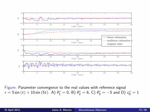
Figure: Parameter convergence to the real values with reference signalr = 5 sin (t) + 10 sin (5t). A) θ∗1 = 0, B) θ∗2 = 6, C) θ∗3 = −5 and D) c∗0 = 1


Persistence of Excitation conditions, with perturbations

0 5 10 15 20 25−4

−3

−2

−1

0

1

2

3

4

Time (sec)

Err

or

0 5 10 15 20 25 30 35 40−4

−3

−2

−1

0

1

2

3

4

Time (sec)

Error

Figure: Tracking error e1 = yp − ym for the classical (left) and the proposed(right) MRAC schemes with reference signal r = 5 cos (t) + 10 cos (5t), withperturbation p (t) = 5 sin (6t).


0 5 10 15 20 25 30 35 40−10

0

10

Time (sec)

0 5 10 15 20 25 30 35 40−10

0

10

Time (sec)

0 5 10 15 20 25 30 35 40−20

0

20

Time (sec)

0 5 10 15 20 25 30 35 40−10

0

10

Time (sec)

Linear estimation

Nonlinear estimation

Real value

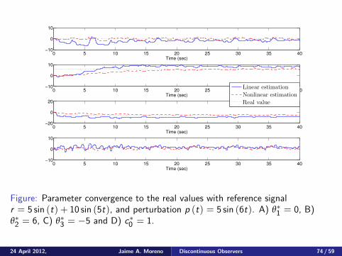
Figure: Parameter convergence to the real values with reference signalr = 5 sin (t) + 10 sin (5t), and perturbation p (t) = 5 sin (6t). A) θ∗1 = 0, B)θ∗2 = 6, C) θ∗3 = −5 and D) c∗0 = 1.


Lack of Persistence of Excitation conditions

0 5 10 15−2

−1

0

1

2

3

4

5

6

7

Time (sec)

ypan

dy m


Plant output

Figure: Model ym (continuous line) and the Plant’s output yp (dotted line) withthe classical MRAC scheme with constant reference signal r = 6.


0 5 10 15−1

0

1

2

3

4

5

6

Time (sec)

y pandy m


Plant output

Figure: Model ym (continuous line) and the Plant’s output yp (dotted line) withthe nonlinear MRAC scheme with reference signal r = 6.


0 5 10 15−15

−10

−5

0

5

10

15

20

Time (sec)

Control

Linear control

Nonlinear control

Figure: Control variable up for the classical MRAC (continuous line) and theproposed nonlinear MRAC (dotted line) with reference signal r = 6.


Adetola, V. and Guay, M. (2008).Finite-time parameter estimation in adaptive control of nonlinearsystems.IEEE Transactions on Automatic Control, 53(3):pp. 807–811.

Davila, J., Fridman, L., and Levant, A. (2005).Second order sliding-modes observer for mechanical systems.IEEE Transactions on Automatic Control, 50(11):pp. 2292–2299.

Davila, J., Fridman, L., and Poznyak, A. (2006).Observation and identification of mechanical systems via second ordersliding modes.Journal of Control., 79(10):pp. 1251–1262.

Ioannou, P. A. and Findan, B. (2006).Adaptive Control Tutorial.Society for Industrial and Applied Mathematics, 3600 University CityScience Center, Philadelphia.


Ioannou, P. A. and Sun, J. (1996).Robust Adaptive Control.Upper Saddle River, NJ.

Levant, A. (1998).Robust exact differentiation via sliding mode technique.Automatica, 34(3):379–384.

Levant, A. (2003).Higher-order sliding modes, differentiation and output-feedbackcontrol.International Journal of Control, 76(9/10):924–941.

Moreno, J. (2009).A linear framework for the robust stability analysis of a generalizedsuper-twisting algotihm.2009 6th International Conference on Electrical Engineering,Computing Science and Automatic Control (CCE 2009)(Formerlyknown as ICEEE), Toluca, Mexico:pp. 10–13.


Morgan, A. P. and Narendra, K. S. (1977).On the stability of nonautonomous differential equationsx = [a + b(t)]x , with skew symmetric matrix b(t).SIAM J. Control and Optimization., 15(1):163–176.

Narendra, K. S. and Annaswamy, A. (1989).Stable Adaptive Systems.Prentice Hall, Englewood Cliffs, NJ.

Sastry, S. and Bodson, M. (1989).Adaptive Control Stability. Convergence and Robustness.Prentice Hall, Englewood Cliffs, NJ.


G. Bastin and D. DochainOn-line estimation and adaptive control of bioreactors.Elsevier, 1990.

Moreno, J.A. and Alvarez, J. and Rocha-Cozatl, E. and Diaz-Salgado,J.Super-Twisting Observer-Based Output Feedback Control of a Classof Continuous Exothermic Chemical ReactorsProceedings of the 9th International Symposium on Dynamics andControl of Process Systems (DYCOPS 2010),Leuven, Belgium, July5-7, 2010,

Farza, M. and Busawon, K. and Hammouri, H.Simple nonlinear observers for on-line estimation of kinetic rates inbioreactorsAutomatica,Vol.34, Num.3, 1998, Elsevier ,


THANKS


Date post:	16-Feb-2022
Category:	Documents
Upload:	others
View:	1 times
Download:	0 times

Discontinuous Observers with strong convergence properties ...

Documents