Our visual world is extraordinarily varied and complex, but despite its rich-ness, the space of visual data may not be that astronomically large. We live in awell-structured, predictable world, where cars almost always drive on roads, sky isalways above the ground, and so on. As humans, the ability to learn this structurefrom prior experiences is essential to our visual perception. In fact, we effortlessly(and often unconsciously) employ this structure for perceiving and responding toour surroundings; a feat that still eludes our computational systems. In this dis-sertation, we propose to discover and harness this structure to improve large-scalevisual recognition systems.
In Part I, we present supervised recognition algorithms that can leverage theseunderlying regularities in our visual world. We propose effective models for objectrecognition that incorporate top-down contextual feedback and models that canleverage geometric-structure of objects. We also develop supervised learning andinference methods that exploit the structure offered by visual data and by a widerange of recognition tasks.
These supervised systems, limited by our ability to collect annotations, areconfined to curated datasets. Therefore, in Part II, we propose to overcome thislimitation by automatically discovering structure in large amounts of visual data andincorporating it as constraints in large-scale semi-supervised learning algorithms toimprove visual recognition systems.
i
Acknowledgments
There are many people, including advisors, collaborators, friends, and family,who have supported and guided me throughout, and to whom I owe deep gratitude.
First and foremost, I thank my advisor, Abhinav Gupta, for always providingme with the right balance of guidance and freedom, at the right time. I appreciatehis consistent support, the time and energy he put in, and above all his patience,during both successes and failures. Though it is impossible to justify his impact onmy growth in a few lines without being reductive; put simply, he has been a closefriend and a fantastic advisor over the last 7 years, and for that, I am immenselyand sincerely grateful.
I’d also like to thank my Masters’ advisors, Alyosha Efros and Martial Hebert,for taking a chance on a young and inexperienced student. They have, generouslyand selflessly, continued to serve as shadow advisors during my Ph.D. I cannotsummarize all that they have done for me; but I especially thank Alyosha for givingme my first break in the field, teaching me never to give up, always pushing meand insisting on excellence, spending long hours late at night helping me with talks,coining my alias ‘A2’, and introducing me to fine spirits; and Martial for teachingme the importance of putting ideas in broader research perspective, exposing me tohands-on real-world applications, trusting me to give demos and presentations tosenior leadership, and making sure that my scotch is without ice!
I cannot overstate the continued impact of Abhinav, Alyosha, and Martial inshaping my research career and outlook since the day I stepped into Carnegie Mellon.I cannot imagine my academic fate had I not been part of their labs, for which Iconsider myself undeservingly fortunate.
Thank you to my thesis committee members, Deva Ramanan and Jitendra Ma-lik, for enlightening discussions, valuable feedback, kind words of encouragement,and flexibility throughout the entire process. I thank David Forsyth for his support,critical insights into my work, and thoughtful suggestions. I am deeply grateful toRahul Sukthankar for his support and guidance all these years which have had aremarkable influence on my career.
iii
It was a pleasure learning from a diverse group of faculty in Smith Hall. I’despecially like to thank Kayvon Fatahalian, Takeo Kanade, Kris Kitani, SrinivasNarasimhan, Yaser Sheikh, and Fernando De la Torre for their time, guidance andencouragement. Thanks to Microsoft Research and Google Research for excellentinternship opportunities; especially Rahul Sukthankar, Mark Segal, Ross Girshick,and Larry Zitnick, for their incredible mentorship.
I owe much to the awesome atmosphere of Smith Hall and the vision andgraphics group members, for whom I have great respect and admiration. Thanksto Aayush Bansal, Nadine Chang, Xinlei Chen, Alvaro Collet, Shreyansh Daftry,Carl Doersch, Santosh Divvala, Ali Farhadi, David Fouhey, Dhiraj Gandhi, RohitGirdhar, Ed Hsiao, Eakta Jain, Hongwen Kang, Abhijeet Khanna, Natasha Khol-gade, Jean-François Lalonde, Yong-Jae Lee, Aravindh Mahendran, Tomasz Mal-isiewicz, Kenneth Marino, Narek Melik-Barkhudarov, Ishan Misra, Lekha Mohan,Yair Movshovitz-Attias, Dan Munoz, Adithya Murali, Ben Newman, Devi Parikh,Lerrel Pinto, Sentil Purushwalkam, Varun Ramakrishna, Olga Russakovsky, ScottSatkin, Gunnar Sigurdsson, Krishna Kumar Singh, Saurabh Singh, Anish Sinha,Ekaterina Taralova, Yuandong Tian, Jack Valmadre, Jacob Walker, Jiuguang Wang,Xiaolong Wang, Yuxiong Wang, Andreas Wendel, Tinghui Zhou, and Jun-Yan Zhu,for discussions, feedback, and friendship. Sincere thanks to my co-authors Ishan,Saurabh, Aayush, Chen, Xiaolong, Tomasz, Elissa, Xinlei, and Carl for their effortsand all those fun all-nighters. I’ve learned a lot from each of you.
Special thanks to: Jean-François, Tomasz, and Alvaro for their instruction dur-ing my early days; Derek, Jean-François, and Yuandong for their advice duringfellowship and job applications; Chen, Ishan, Saurabh, and Sean for a great in-ternship experience; Abhinav, David, Saurabh, and Ishan for making conferencesmemorable; David and Ishan for helping with talks and proof-reading; Abhinav,Bhavna, Dan, David, Dev, Dey, Ermine, Govind, Hatem, Ishan, Jack, Natasha,Nandita, Ravi, Saloni, Saurabh, Shannon, Shaurya, Swati, Varun, Varuni, and Zeelfor some unforgettable parties. Shout-out to the coffee gang (Abhinav, David, andIshan) and movie knights (Jiuguang, Dey, Natasha, Saurabh) for a great time!
The Robotics Institute and CMU provides an incredibly nurturing environmentfor a graduate student. Particular thanks to Rachel Burchin for being a friendand advisor and helping navigate the immigration maze, Suzanne Lyons Muth forkeeping me on track, Lynnetta Miller, Christine Downey, and Jessica Butterbaughfor all their help and patience, Byron Spice for helping with media outreach, SCSComputing Facilities (especially EdWalter and Bill Love) for maintaining the serversand keeping up with my untimely requests and unannounced meetings.
iv
I am also indebted to my late uncle, Abhay Shrivastava, without whose guidanceI would not have pursued a research career, and to my undergraduate mentor, SanjayGoel, for motivating me to pursue my passion. Thanks to all my teachers for theirkind words, encouragement, and support.
I’ve been incredibly lucky to be surrounded by many supportive friends, whohave kept me sane during some insane times. For being my family away from home,I’d like to thank: Ashima, Shannon, & Dey; Samhita, Harshita, & Saurabh; Saloni& Ishan; Skip, Swati, & Abhinav; Zeel & Ravi; Manali, Anubha, Akshat, Anurag,& Varun Saxena. Thanks to: Saurabh and Harshita for hosting and feeding meduring my Bay Area visits; David for hosting me at Berkeley; Virag Mama forLaphroaig 30, and much more, which made Bay Area visits particularly fun; friendsand colleagues in Bay Area (especially Varun Somani, Ridhima, Rashmi, Ashwath,Rishabh, Amrita, Sean, and Himanshu) for always finding time for me; dear friendselsewhere (Anubhav, Neha Kumar, Aparna, Kripi, Robin, Shalini, Adit, Ashmita,Saurabh Aswani, Sonal, and everyone else), for always being a phone call away, nomatter for how long we haven’t talked. Thanks to everyone who has ever served mecaffeine, wine, and scotch, for this dissertation was written in between sips. Specialthanks to Ishan, Dey, Saurabh, and Anubhav for always being there.
Finally, I’d like to thank my family and extended family, without whose supportI could not have finished this thesis. I thank my parents and sister for their never-ending love and support throughout all these years. Thank you, Mom and Dad,for your sacrifices and encouragement which enabled me to follow my dreams. Andlast, but certainly not the least, I thank my wife, Varuni, for selfless sacrifice, quietpatience, unwavering support, and unconditional love. Thank you, Varuni, for beingmy partner in crime, bearing with my erratic schedules, sticking with me throughthick and thin, and constantly motivating me to achieve more.
Thank you all for believing in me, even when I did not.
v
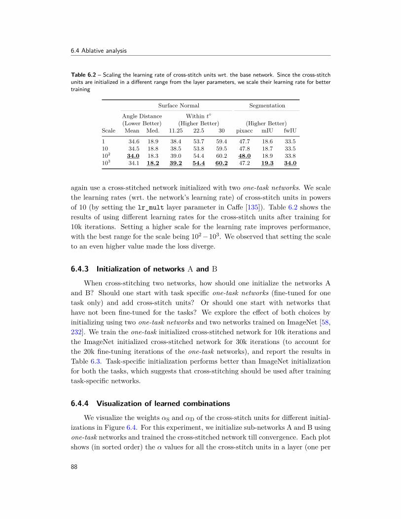
Credits. This work has been partially supported by a Microsoft Research PhD Fel-lowship, ONR grants: N000141010766, MURI N000141612007, MURI N000141010934,and MURI N000141612007, NSF grants IIS-1320083 and IIS-1065336, ARL grantCTA W911NF-10-2-0016, and gifts from Google and Bosch. We’d also like to thankYahoo! and NVIDIA for hardware donations. Image credits (Chapter 7): Char-alampos Laskaris, Carol Williams, Claudio Conforti, Eddie Wong, Edson Campos,Prof. Hall Groat II, Kathleen Brodeur, Moira Munro, Matt Wyatt, Keith Horn-blower, Don Amadio (Scrambled Eggz Productions), The Stephen Wilthsire Gallery,www.daydaypaint.com, The Art Renewal Center and Bundesarchiv. We thank theFlickr users who placed their work under Creative Commons License, researcherswho collected and released datasets and made their code available online.
We humans have the remarkable ability to perceive and operate in the visualworld around us. For example, recognizing our favorite cookie on a heavily cluttereddinner table is hardly a challenge for us. However, the same task is herculean fora robot, despite tremendous advancement in artificial intelligence over the years.This dissertation is about bringing computational systems closer to operating insuch real-world scenarios. Our primary focus is developing computation modelsand algorithms for Visual Recognition, the problem of identifying and reasoningabout concepts within an image, which is one of the key challenges in computervision and artificial intelligence.
Our visual world is extraordinarily varied and complex, but despite its rich-ness, the space of visual data may not be that astronomically large. We live in awell-structured, predictable visual world, where cars almost always drive on roads,plates are kept on dining-tables, sky is always above the ground, televisions andpaintings usually have rectangular fronts, beds and tables have horizontal surfaces,and so on. As humans, the ability to learn these regularities, or structure, fromprior experiences is essential to our visual perception [294]. This structure not onlyacts as top-down contextual feedback in our visual system, but also facilitates rea-soning when visual information is insufficient. In fact, we effortlessly (and oftenunconsciously [294]) employ this structure for perceiving and responding to our sur-roundings; a feat that still eludes our artificial systems. I firmly believe the better asystem is at discovering, learning, and exploiting this inherent structure, the better
1
1. Introduction
it will be at understanding and reacting to the visual world.
Driven by this hypothesis, this dissertation proposes to discover and harnessthis structure in the visual data to enable large-scale visual recognition.
The last decade has seen tremendous advances in visual recognition algorithms.This progress has been primarily fueled by massive efforts by researchers in thefield to collect human-annotations (in terms of labeled instances of scenes, objects,actions, attributes etc.) for large amounts of visual data available online (images,videos, etc.). This supervised learning paradigm is the backbone of today’s visualrecognition algorithms. Therefore, the first part of this dissertation is on:
I. Supervised Visual Recognition, where we propose computational modelsand learning algorithms that enable these supervised recognition systems toleverage the underlying regularities in our visual world. This includes:
(a) Models for object recognition; such as models that can incorpo-rate the visual structure using top-down contextual feedback and achievestate-of-the-art results on challenging benchmarks (Chapters 2 and 3),and models that leverage the 3D structure and provide a geometric un-derstanding of objects from 2D images (Chapter 5).
(b) Optimization and inference methodologies that utilize the struc-ture in visual data; such as algorithms that can effectively leverage task-specific problem structure (Chapter 4), underlying 3D structure of objects(Chapter 5), shared structure between multiple tasks (Chapter 6).
The two ingredients required by these supervised learning algorithms, visualdata and human-annotations, vary greatly in their availability and cost. While visualdata is abundant and cheap (due to increasingly inexpensive sensors, computation,and storage), human-provided labels, in comparison, are scant and expensive. Forexample, annotating one of the largest vision dataset (ImageNet), which contains∼1 million images with bounding-box labels, took over 5 years (using 19 man-years). This might seem impressive if it were not for the fact that ∼350 millionnew images are uploaded to Facebook daily and 300 hours of video are uploadedto YouTube every minute. In all likelihood, manual labeling cannot possibly scaleto the ever increasing amounts of visual data. Therefore, limited by our ability tocollect annotations, current systems are confined to curated datasets.
An obvious solution is to circumvent this labeling bottleneck and do the follow-ing: a) train supervised models using the already labeled data, b) use these models tofind similar concepts in unlabeled data and label it, and c) continue doing this untileverything is labeled. This is the classic semi-supervised learning paradigm, which
2
1.1 Overview
has been quite promising in several domains. However, semi-supervised approachesare often not reliable when applied to visual data. The primary reason is that oursupervised visual models are not perfect. Hence, the notion of similarity as capturedby these visual models (i.e., deciding if two images depict visually similar informa-tion or concept), which is a critical requirement for any semi-supervised method, isnot very reliable for visual data. This often leads to newly labeled examples strayingaway from the original meaning of the concept (semantic drift).
So, the key question is: how do we reduce the reliance of our recognition systemson carefully annotated datasets and enable them to harness the sea of unlabeledvisual data? To answer this, the second part of this dissertation focuses on:
II. Recognition beyond Extensive Supervision. We propose systems thatleverage the underlying structure in our visual data to overcome the limita-tions highlighted above and capitalize on large-scale unlabeled visual data.This includes learning frameworks (Chapters 7 and 8) that incorporate thisstructure as constraints, and systems that discover and learn this structurecontinuously from millions of images and videos (Chapter 9).
1.1 OverviewMost of the complex structures found in theworld are enormously redundant, and we canuse this redundancy to simplify their description.But to use it, to achieve the simplification,we must find the right representation.
Herbert A. Simon
The organization of this thesis follows the two-pronged strategy for discoveringand leveraging the regularities in our visual data. In Part I, we present supervisedrecognition models and learning algorithms, with various flavors of labeled data andtarget tasks. In Part II, we show how to reduce the reliance on extensive human-provided annotations and leverage large amounts of unlabeled data to improve visualrecognition systems. We describe the problem setup for each Chapter in both Partsand their key insights below.
Identifying and localizing objects in a scene, or Object Recognition, is at theheart of visual perception; and representations from bottom-up, feedforward Convo-lutional Networks (ConvNets) are the backbone of recent object recognition systems.However, studies in human perception suggest the importance of top-down informa-tion, context, and feedback for object recognition [154]. Drawing inspiration fromthis, in Chapters 2 and 3, we propose novel ConvNet representations with top-down
3
1.1 Overview
person
boat
person
dinningtable
person
personpersonperson
dinningtable
bottle
Figure 1.1 – Qualitative results from Chapter 2 (top row) and Chapter 3 (bottom row).
feedback that enable recognition systems to leverage contextual structure in visualdata. These models, originally introduced in [250, 254], are one of the first to reportsignificant quantitative improvements on various recognition tasks by incorporatingtop-down evidence.
In Chapter 2, we show how semantic segmentation outputs (per-pixel likeli-hood of objects) can be used as a proxy for top-down information. We argue that asegmentation output captures contextual relationships between objects (such as rel-ative likelihood, location, and size) and use it for contextual priming and providingfeedback. Our results indicate that such top-down priming improves the perfor-mance on object detection, semantic segmentation, and region proposal generation.Qualitative results on semantic segmentation are shown in Figure 1.1 (top row).Current recognition systems, including Chapter 2, rely on the high-level semanticrepresentations from ConvNets, which, by design, are invariant to low-level details.These fine details are often essential to recognize many objects; e.g., finding the‘remote’ in cluttered ‘livingroom’ in Figure 1.1 (bottom row). To address this, weintroduce top-down modulation network in Chapter 3, which utilizes top-down con-textual structure to modulate and select low-level finer details, and integrates themwith the high-level semantic representation for object recognition. The proposednetwork provides substantial gains in recognition rates for various ConvNet archi-tectures, yielding state-of-the-art results on the challenging COCO object detectiondataset (Qualitative detection results are shown in Figure 1.1 (bottom row)).
The object detection frameworks discussed in Chapters 2 and 3 are trainedusing techniques developed for object classification, where the goal is to identify thepresence of objects in an image, and not localize them. To adapt these techniquesfor localization, several heuristics and hyperparameters are used which are sub-optimal and costly to tune. These heuristics are primarily used to address the issuethat detection datasets contain an overwhelming number of easy examples and asmall number of hard examples. Instead of using costly heuristics, in Chapter 4, we
4
1.1 Overview
Input Image G-DPM Detection Predicted Geometry
Figure 1.2 – Qualitative result from Chapter 5.
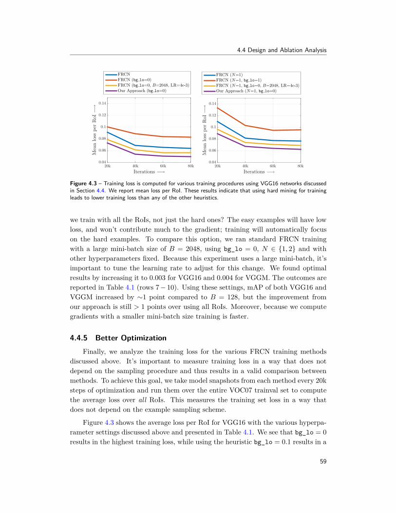
present a simple and intuitive online hard example mining algorithm that leveragesthe detection-specific problem structure when training ConvNet-based models ina principled way and enables automatic selection of these hard examples. Thisnot only simplifies the training procedure, but also makes it more effective andefficient. More importantly, it yields consistent and significant boosts in detectionperformance on benchmarks like PASCAL VOC 2007, 2012 and MS COCO. Thiswork, originally introduced in [253], is being used by the community for trainingstate-of-the-art systems for object detection, semantic and instance segmentation.
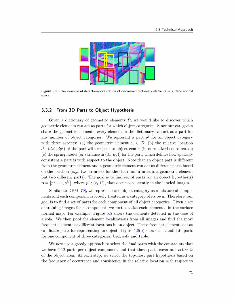
Next, we look at how we can use the underlying geometry of objects to imposestructure while training detection models in Chapter 5. The standard output ofobject recognition systems discussed so far is either a box around the localized object(detection) or per-pixel labels (segmentation). Though critical building blocks, theseoutputs offer a rather shallow understanding of the recognized object. In Chapter 5,we propose a system to infer 3D properties of objects from 2D images. Our modelfirst automatically discovers the geometric structure of an object and its parts usingmulti-model input (images + depth). During training, we enforce that the modelfollows this geometric structure. The model is trained only for 2D images, anddepth is only used to provide geometric constraints. Therefore, during inference, themodel only needs images (and no depth). These geometry-constrained deformablepart-based models (G-DPM), originally introduced in [249], provide state-of-the-artperformance on the NYUv2 dataset (Figure 1.2).
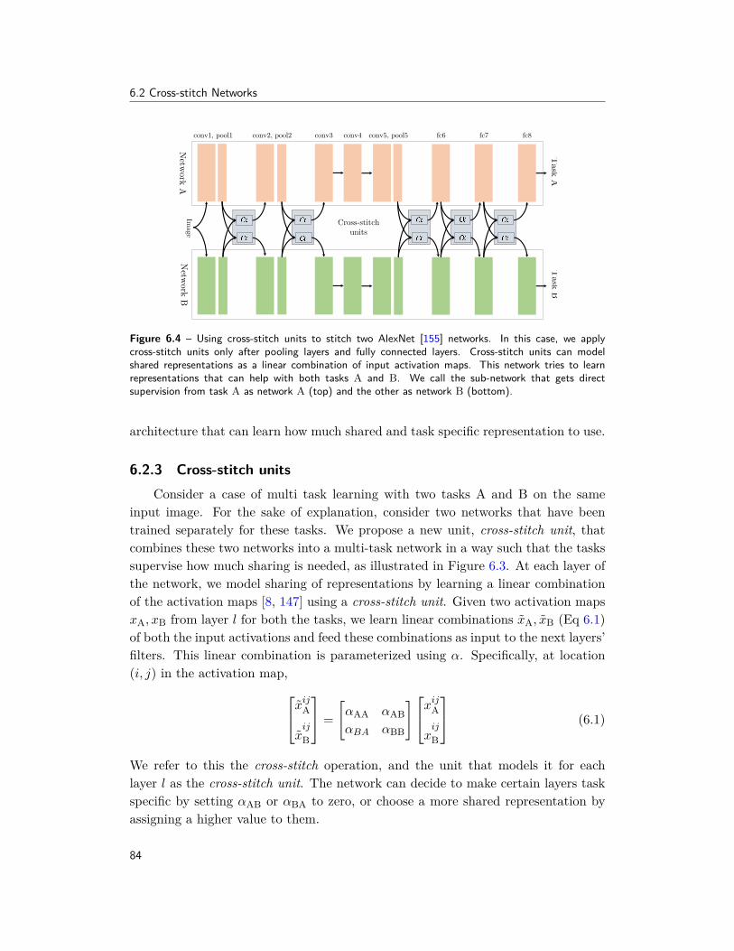
In Chapter 5, we proposed a model to better utilize images and depth dataduring training. Next, we look at a more generic setup of multi-task learning,where we jointly utilize multiple supervisory labels for training recognition models(e.g., labels for scenes, objects, attributes, depth, etc.). ConvNets trained usingmulti-task learning have been widely successful in the field of recognition, primarilybecause having multiple tasks forces the model to learn shared representation suit-able for both tasks. However, existing multi-task approaches rely on enumeratingmultiple ConvNet architectures, which are specific to the tasks at hand and do notgeneralize. In Chapter 6, we propose a principled approach to learn such sharedrepresentation, which automatically discovers optimal combination of shared and
5
1.1 Overview
task-specific representations via “cross-stitch” units. Our method generalizes acrossmultiple tasks and shows dramatically improved performance for categories withfew training examples. This work, originally presented in [193], highlights the im-portance of leveraging structure between tasks for learning shared representations.
So far, in Part I, we have seen how to improve supervised recognition models byleveraging the structure in visual data. In Part II, we present methods for discoveringthis structure automatically from large-amounts of visual data, and leveraging it toimprove recognition algorithms. Towards this, we develop systems that utilize datawith varying granularity of labeling, such as weak and noisy labels (Chapter 9),sparse and partial labels (Chapters 8 and 9), or no labels at all (Chapter 7).
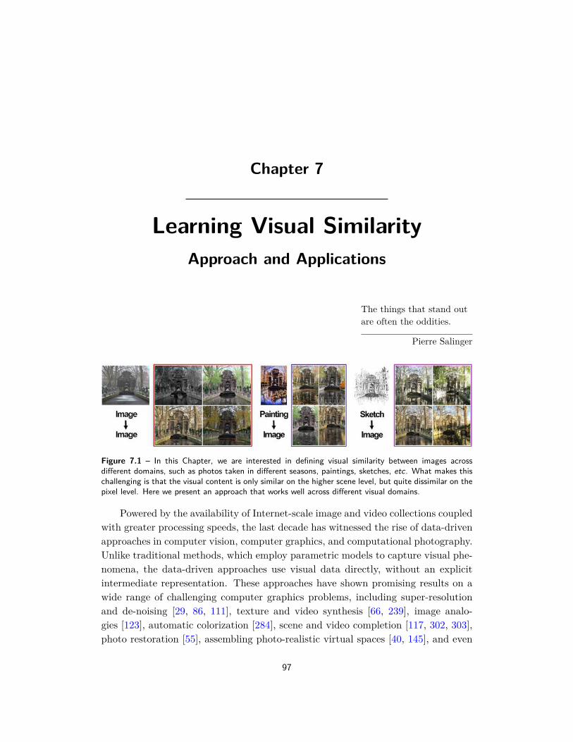
In Chapter 7, we start with the simplest setting, where we are given only a singlelabeled instance of a concept, without any explicit negatives (or images without anyconcepts labeled), and the goal is to learn a good visual similarity metric. A criticalcomponent of finding recurring patterns in ‘big visual data’ is matching images, orparts thereof, with each other. However, this is surprisingly challenging because thenotion of similarity, required for matching, is ill-defined. We present a simple visualsimilarity metric based on notion of “data-driven uniqueness,” which estimates therelative importance of different features of an image based on what best distinguishesit from the statistical structure of millions of images. This visual similarity showsgood performance on a number difficult cross-domain visual tasks, e.g., matchingpaintings or sketches to real photographs.
In Section 7.4, we briefly discuss applications of this improved visual similarity,such as Internet Re-photography and Painting2GPS in Section A1, organization andexploration of unordered large-scale visual data in Section A2, and finally discoveringobject instances and their segmentation masks from weakly-supervised and noisyweb data in Section A3. These works were originally presented in [42, 186, 251].
Finally, in Chapters 8 and 9, we tackle the problem of effectively utilizing largeamounts of unlabeled data along with a small amount of labeled data, i.e., thesemi-supervised learning (SSL) paradigm. We present recognition algorithms thatdiscover the visual structure from labeled data and use it as constraints in an SSLframework, to capitalize on large amounts of unlabeled visual data. These workswere originally presented in [41, 192, 252].
In Chapter 8, we begin with a case study of a proof-of-concept system, wherewe study how to incorporate different types of constraints, and their importance, inan SSL framework. We start with a small list of scene categories and manually pro-vide annotated instances and associated constraints. The constraints are providedin the form of attribute and comparative attribute labels for the scenes. To incor-
6
1.1 Overview
Input Painting Estimated Geo-locationGoogle’s Top Matches
Figure 1.3 – Qualitative results from Part II. (a) Image retrieval results using similarity metric (Chap-ter 7); (b) Painting2GPS (Chapter 7 Section A1); (c) Learned object recognition priors from weakly-supervised and noisy web data (Chapter 7 Section A3); (d) Learned visual relationships (Chapter 9).
porate these constraints, we propose a mathematical framework ‘constrained-SSL,’which can train good recognition models even when starting from just two labeledinstances; while the standard SSL approaches suffer severe semantic drift. Thiswork, presented in [252], was one of the first to reliably utilize SSL for large-scalerecognition (with an unlabeled dataset of millions of images).
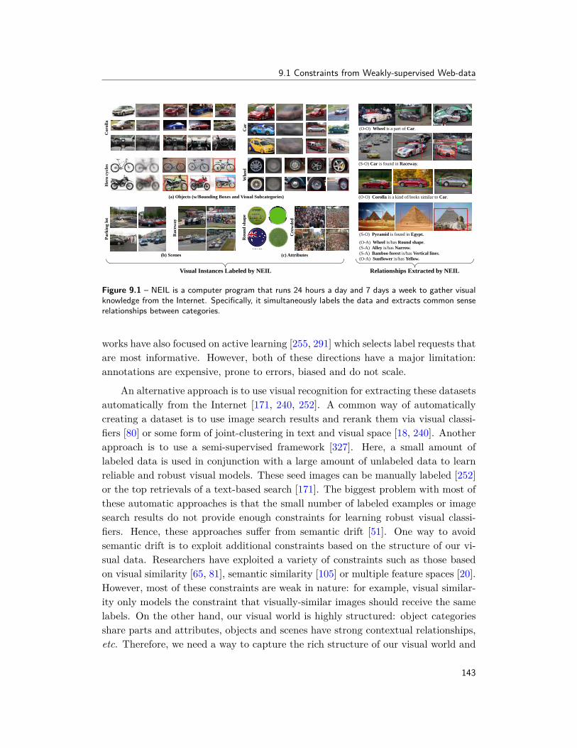
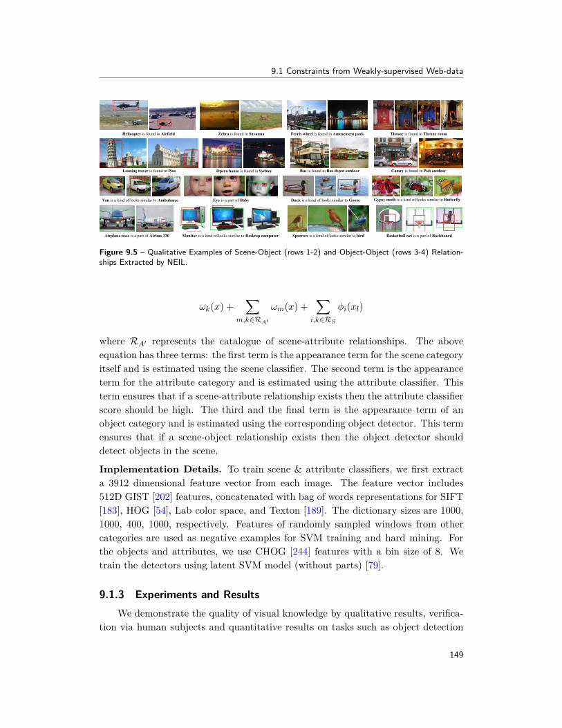
In Chapter 9, we propose to apply the ideas from this case study to real worldscenarios. In Section 9.1, we propose a system that can learn these constraints fromweakly-supervised, noisy web-data. We extend the list of concepts to scenes, objectsand attributes, and type of constraints to scene-object, object-object, scene-attributeand object-attribute relationships. We show that these automatically discoveredrelationships are good for constrained SSL. We only provided relevant details inSection 9.1, other details can be found in [41]. In Section 9.2, we demonstratehow constraints can be discovered and harnessed in large-scale videos, where onlya handful of frames are sparsely labeled with concepts. The proposed techniquehandles detection of multiple objects without assuming exhaustive labeling of objectinstances on any input frame; and starting with a handful of labeled examples, itcan label hundreds of thousands of new examples. The models trained with thesediscovered examples result in much better recognition rates, across multiple videodatasets. Again, we only provided relevant details in Section 9.2, other details canbe found in [192].
Finally, we summarize the contributions of this thesis, include a discussion onfuture directions it enables, and put this dissertation in the broader context of thefast-paced field of Visual Recognition.
7
Part I
Supervised Visual Recognition
Chapter 2
Contextual Priming & Feedback
The situation has provided a cue; this cue has giventhe expert access to information stored in memory,and the information provides the answer. Intuitionis nothing more and nothing less than recognition.
Herbert A. Simon
The field of object recognition has changed drastically over the past few years.We have moved from manually designed features [54, 79] to learned ConvNet fea-tures [96, 119, 155, 258]; from the original sliding window approaches [79, 292] toregion proposals [95, 96, 103, 223, 298]; and from pipeline based frameworks such asRegion-based CNN (R-CNN) [96] to more end-to-end learning frameworks such asFast [95] and Faster R-CNN [223]. The performance has continued to soar higher,and things have never looked better. There seems to be a growing consensus – pow-erful representations learned by ConvNets are well suited for this task, and designingand learning deeper networks lead to better performance.
Most recent gains in the field have come from bottom-up, feedforward frame-work of ConvNets. On the other hand, in the case of human visual system, thenumber of feedback connections significantly outnumber the feedforward connec-tions. In fact, many behavioral studies have shown the importance of context andtop-down information for the task of object detection. This raises a few importantquestions – Are we on the right path as we try to develop deeper and deeper, butonly feedforward networks? Is there a way we can bridge the gap between empiricalresults and theory, when it comes to incorporating top-down information, feedbackand/or contextual reasoning in object detection?
This Chapter investigates how we can break the feedforward mold in currentdetection pipelines and incorporate context, feedback and top-down information.
11
2. Contextual Priming & Feedback
Current detection frameworks have two components: the first component generatesregion proposals and the second classifies them as an object category or background.These region proposals seem to be beneficial because (a) they reduce the searchspace; and (b) they reduce false positives by focusing the ‘attention’ in right areas.In fact, this is in line with the psychological experiments that support the idea ofpriming (although note that while region proposals mostly use bottom-up segmen-tation [7, 103], top-down context provides the priming in humans [190, 287, 304]).So, as a first attempt, we propose to use top-down information in generating regionproposals. Specifically, we add segmentation as a complementary task and use it toprovide top-down information to guide region proposal generation and object detec-tion. The intuition is that semantic segmentation captures contextual relationshipsbetween objects (e.g., support, likelihood, size etc. [19]), and can guide the regionproposal module to focus attention in the right areas and learn detectors from them.
But contextual priming using top-down attention mechanism is only part of thestory. In case of humans, the top-down information provides feedback to the wholevisual pathway (as early as V1 [130, 154]). Therefore, we further explore providingtop-down feedback to the entire network in order to modulate feature extractionin all layers. This is accomplished by providing the semantic segmentation outputas input to different parts of the network and training another stage of our model.The hypothesis is that equipping the network with this top-down semantic feedbackwould guide the visual attention of feature extractors to the regions relevant for thetask at hand.
To summarize, we propose to revisit the architecture of a current state-of-the-art detector (Faster R-CNN [223]) to incorporate top-down information, feedbackand contextual information. Our new architecture includes:
• Semantic Segmentation Network: We augment Faster R-CNN with asemantic segmentation network. We believe this segmentation can be used toprovide top-down feedback to Faster R-CNN (as discussed below).
• Contextual Priming via Semantic Segmentation: In Faster R-CNN,both region proposal and object detection modules are feedforward. We pro-pose to use semantic segmentation to provide top-down feedback to thesemodules. This is analogous to contextual priming; in this case top-down se-mantic feedback helps propose better regions and learn better detectors.
• Iterative Top-Down Feedback: We also propose to use semantic segmen-tation to provide top-down feedback to low-level filters, so that they becomebetter suited for the detection problem. In particular, we use segmentation asan additional input to lower layers of a second round of Faster R-CNN.
12
2.1 Related Work
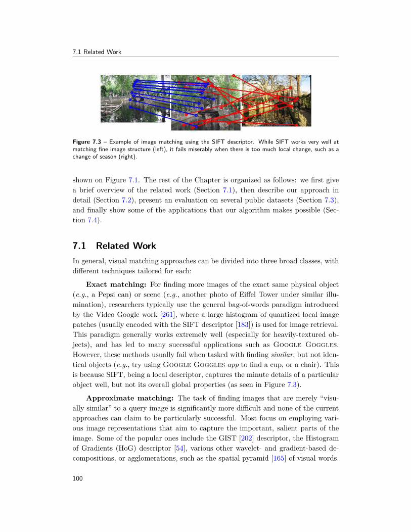
2.1 Related WorkObject detection was once dominated by the sliding window search paradigm [79,292]. Soon after the resurgence of ConvNets for image classification [58, 155, 167],there were attempts at using this sliding window machinery with ConvNets [71, 243,270]; but a key limitation was the computational complexity of brute-force search.
As a consequence, there was major paradigm shift in detection which com-pletely bypassed the exhaustive search in favor of region-based methods and objectproposals [4, 4, 7, 32, 69, 103, 288, 329]. By reducing the search space, it al-lowed us to use sophisticated (both manually designed [48, 83, 298] and learnedConvNet [16, 96, 115, 116, 120, 180, 223]) features. Moreover, this also helped fo-cus the attention of detectors to regions well supported by perceptual structures inthe image. However, recently, Faster R-CNN [223] showed that even these regionproposals can be generated by using ConvNet features. It removed segmentationfrom proposal pipeline by training a small network on top of ConvNet features thatproposes a few object candidates. This raises an important question: Do ConvNetfeatures already capture the structure that was earlier given by segmentation ordoes segmentation provide complementary information?
To answer this, we study the impact of using semantic segmentation in theregion proposal and object detection modules of Faster R-CNN [223]. In fact, therehas been a lot of interest in using segmentation in tandem with detection [42, 48,64, 83]; e.g., Fidler et al. [83] proposed to use segmentation proposals as additionalfeatures for DPM detection hypothesis. In contrast, we propose to use semanticsegmentation to guide/prime the region proposal generation itself. There is ampleevidence of the importance of similar top-down contextual priming in the humanvisual system [57, 190], and its utility in reducing areas to focus our attention onfor recognizing objects [287, 304].
This prevalence and success of region proposals is only part of the story. An-other key ingredient is the powerful ConvNet features [119, 155, 258]. ConvNetsare multi-layered hierarchical feature extractors, inspired by visual pathways in hu-mans [78, 154]. But so far, our focus has been on designing deeper [119, 258]feedforward architectures, even when there is a broad agreement on the importanceof feedback connections [47, 94, 130] and limitations of purely feedforward recogni-tion [161, 307] in human visual systems. Inspired by this, we investigate how canwe start incorporating top-down feedback in our current object detection architec-tures. There have been attempts earlier at exploiting feedback mechanisms; somewell known examples are auto-context [286] and inference machines [228]. Theseiteratively use predictions from a previous iteration to provide contextual features
13
2.2 Preliminaries: Faster R-CNN
to the next round of processing; however they do not trivially extend to ConvNetarchitectures. Closest to our goal are the contemporary works on using feedback tolearn selective attention [194, 265] and using top-down iterative feedback to improveat a task at hand [33, 89, 170]. In this work, we additionally explore using top-downfeedback from one task to another.
The discussion on using global top-down feedback to contextually prime objectrecognition is incomplete without relating it to ‘context’ in general, which has along history in cognitive neuroscience [19, 124, 127, 190, 203, 204, 287, 304] andcomputer vision [59, 88, 197, 219, 280, 281, 282, 314]. It is widely accepted thathuman visual inference of objects is heavily influenced by ‘context’, be it contextualrelationships [19, 124], priming for focusing attention [190, 287, 304] or importanceof scene context [57, 127, 203, 204]. These ideas have inspired lot of computervision research (see [59, 88] for survey). However, these approaches seldom lead tostrong empirical gains. Moreover, they are mostly confined to weaker visual features(e.g., [54]) and have not been explored much in ConvNet-based object detectors.
For region-based ConvNet object detectors, simple contextual features are slowlybecoming popular; e.g., computing local context features by expanding the re-gion [93, 195, 196, 328], using other objects (e.g., people) as context [110] and usingother regions [98]. In comparison, the use of context has been much more popularfor semantic segmentation. E.g., CRFs are commonly used to incorporate contextand post-process segmentation outputs [39, 241, 323] or to jointly reason about re-gions, segmentation and detection [158, 328]. More recently, RNNs have also beenemployed to either integrate intuitions from CRFs [174, 212, 323] in end-to-endlearning systems or to capture context outside the region [16]. But empirically, atleast for detection, such uses of context have mostly given feeble gains.
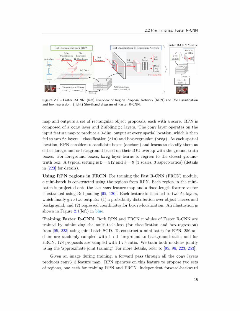
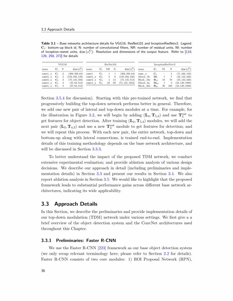
2.2 Preliminaries: Faster R-CNNWe first describe the two core modules of the Faster R-CNN [223] framework (Fig-ure 2.1). The first module takes an image as input and proposes rectangular regionsof interest (RoIs). The second module is the Fast R-CNN [95] (FRCN) detector thatclassifies these proposed regions. In this Chapter, both modules use the VGG16 [258]network, which has 13 convolutional (conv) and 2 fully connected (fc) layers. Bothmodules share all conv layers and branch out at conv5_3. Given an arbitrary sizedimage, the last conv feature map (conv5_3) is used as input to both the modulesas described below.
Region Proposal Network (RPN). The region proposal module (Figure 2.1(left)in green) is a small fully convolutional network that operates on the last feature
14
2.2 Preliminaries: Faster R-CNN
Convolutional Filters conv1_1 – conv4_3
Activation Maps(conv5_1 - conv5_3)
3x3 Conv
…
··
·
· ·
k Anchors 2k Scores 4k Coordinates
fg-bgClassification
BboxRegression
RoIPooling Layer
fcLayers
Cls. Loss
BboxReg. Loss
For each RoI
RoISampler
RoI Proposal Network (RPN) RoI Classification & Regression Network
Pool4, /2
conv5_1
conv5_2
conv5_3
RPNModule
RoI Cls& BReg
Conv5_3
conv1_1 –conv4_3
Pool4, /2
Faster R-CNN Module
Figure 2.1 – Faster R-CNN. (left) Overview of Region Proposal Network (RPN) and RoI classificationand box regression. (right) Shorthand diagram of Faster R-CNN.
map and outputs a set of rectangular object proposals, each with a score. RPN iscomposed of a conv layer and 2 sibling fc layers. The conv layer operates on theinput feature map to produce a D-dim. output at every spatial location; which is thenfed to two fc layers – classification (cls) and box-regression (breg). At each spatiallocation, RPN considers k candidate boxes (anchors) and learns to classify them aseither foreground or background based on their IOU overlap with the ground-truthboxes. For foreground boxes, breg layer learns to regress to the closest ground-truth box. A typical setting is D = 512 and k = 9 (3 scales, 3 aspect-ratios) (detailsin [223] for details).
Using RPN regions in FRCN. For training the Fast R-CNN (FRCN) module,a mini-batch is constructed using the regions from RPN. Each region in the mini-batch is projected onto the last conv feature map and a fixed-length feature vectoris extracted using RoI-pooling [95, 120]. Each feature is then fed to two fc layers,which finally give two outputs: (1) a probability distribution over object classes andbackground; and (2) regressed coordinates for box re-localization. An illustration isshown in Figure 2.1(left) in blue.
Training Faster R-CNN. Both RPN and FRCN modules of Faster R-CNN aretrained by minimizing the multi-task loss (for classification and box-regression)from [95, 223] using mini-batch SGD. To construct a mini-batch for RPN, 256 an-chors are randomly sampled with 1 : 1 foreground to background ratio; and forFRCN, 128 proposals are sampled with 1 : 3 ratio. We train both modules jointlyusing the ‘approximate joint training’. For more details, refer to [95, 96, 223, 253].
Given an image during training, a forward pass through all the conv layersproduces conv5_3 feature map. RPN operates on this feature to propose two setsof regions, one each for training RPN and FRCN. Independent forward-backward
15
2.3 Our Approach
passes are computed for RPN and FRCN using their region sets, gradients areaccumulated at conv5_3 and back-propagated through the conv layers.
Why Faster R-CNN? Apart from being the current state-of-the-art object de-tector, Faster R-CNN is also the first framework that learns where to guide the‘attention’ of an object detector along with the detector itself. This end-to-endlearning of proposal generation and object detection provides a principled testbedfor studying the proposed top-down contextual feedback mechanisms.
In the following Sections, we first describe how we add a segmentation moduleto Faster R-CNN (Section 2.3.1) and then present how we use segmentation fortop-down contextual priming (Section 2.3.2) and iterative feedback (Section 2.3.3).
2.3 Our ApproachWe propose to use semantic segmentation as a top-down feedback to the RPN andFRCN modules in Faster R-CNN, and iteratively to the entire network. We arguethat a raw segmentation output is a compact signal that captures the desired contex-tual information, such as relationships between objects, along with global structuresin the image; and hence is a good representation for top-down feedback.
2.3.1 Augmenting Faster R-CNN with SegmentationThe first step is to augment Faster R-CNN framework with an additional seg-
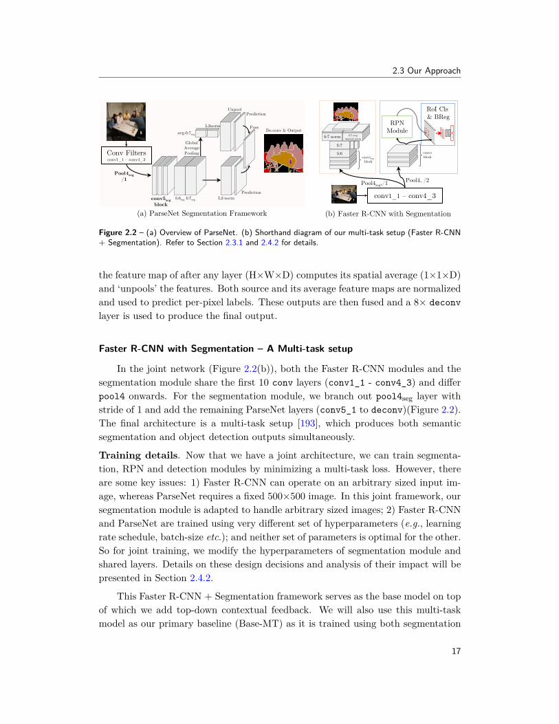
mentation module. This module should ideally: 1) be fast, so that we do not giveup the speed advantages of [95, 223]; 2) closely follow the network used by FasterR-CNN (VGG16 in this Chapter), for easy integration; and 3) use minimal (prefer-ably no) post-processing, so that we can train it jointly with Faster R-CNN. Outof several possible architectures [12, 39, 178, 180, 323], we choose the ParseNetarchitecture [178] because of the simplicity.
ParseNet [178] is a fully convolutional network [180] for segmentation. It isfast because it uses filter rarefication technique (a-trous algorithm) from [39]. Itsarchitecture is similar to VGG16. Moreover, it uses no post-processing; and insteadadds an average pooling layer to incorporate global context; which is shown to havesimilar benefits to using CRFs [39, 174].
Architecture details. An overview is shown in Figure 2.2(a). The key differencefrom standard VGG16 is that the pooling after conv4_3 (pool4seg) does no down-sampling, as opposed to the standard pool4 which down-samples by a factor of 2.After the conv5 block, it has two 1×1 conv layers with 1024 channels applied witha filter stride [39, 178]. Finally, it has a global average pooling step which given
16
2.3 Our Approach
Conv Filters conv1_1 – conv4_3
Pool4seg
/1
conv5seg
block
avg-fc7seg
GlobalAveragePooling
L2-norm
L2norm
UnpoolPrediction
FuseDe-conv & Output
Prediction
fc7segfc6seg
(a) ParseNet Segmentation Framework (b) Faster R-CNN with Segmentation
conv1_1 – conv4_3
Pool4seg,/1Pool4, /2
fc6
fc7
conv5seg
block
fc7 norm fc7-avgunpool-norm
conv5
block
RPNModule
RoI Cls& BReg
Figure 2.2 – (a) Overview of ParseNet. (b) Shorthand diagram of our multi-task setup (Faster R-CNN+ Segmentation). Refer to Section 2.3.1 and 2.4.2 for details.
the feature map of after any layer (H×W×D) computes its spatial average (1×1×D)and ‘unpools’ the features. Both source and its average feature maps are normalizedand used to predict per-pixel labels. These outputs are then fused and a 8× deconvlayer is used to produce the final output.
Faster R-CNN with Segmentation – A Multi-task setup
In the joint network (Figure 2.2(b)), both the Faster R-CNN modules and thesegmentation module share the first 10 conv layers (conv1_1 - conv4_3) and differpool4 onwards. For the segmentation module, we branch out pool4seg layer withstride of 1 and add the remaining ParseNet layers (conv5_1 to deconv)(Figure 2.2).The final architecture is a multi-task setup [193], which produces both semanticsegmentation and object detection outputs simultaneously.
Training details. Now that we have a joint architecture, we can train segmenta-tion, RPN and detection modules by minimizing a multi-task loss. However, thereare some key issues: 1) Faster R-CNN can operate on an arbitrary sized input im-age, whereas ParseNet requires a fixed 500×500 image. In this joint framework, oursegmentation module is adapted to handle arbitrary sized images; 2) Faster R-CNNand ParseNet are trained using very different set of hyperparameters (e.g., learningrate schedule, batch-size etc.); and neither set of parameters is optimal for the other.So for joint training, we modify the hyperparameters of segmentation module andshared layers. Details on these design decisions and analysis of their impact will bepresented in Section 2.4.2.
This Faster R-CNN + Segmentation framework serves as the base model on topof which we add top-down contextual feedback. We will also use this multi-taskmodel as our primary baseline (Base-MT) as it is trained using both segmentation
17
2.3 Our Approach
(a) Contextual Priming Model (b) Iterative Feedback Model
Append
RPNModule
Segmentation
conv1_1 – conv4_3
Norm/Pool
Segmentation Module
conv4_3
Seg.+conv4_3
RoI Cls. & BReg.
Seg.+Pool5
Pool5 fc6
conv5_3
Append
Norm/Pool
RPNModule
RoI Cls& BReg
Norm/Pool
Norm/Pool
conv1_1 – conv4_3
Segmentation Module
Segmentation
Image
Norm
AppendAppendAppend
Norm/Pool
conv1 blockconv2 block
conv3 block conv4 block
Append
conv1_1 – conv4_3
Segmentation Module
Image
Stage 1 Stage 2
RPNModule
RoI Cls& BReg
N/P
A
RPNModule
conv1_1 – conv4_3
Segmentation Module
RoI Cls& BReg
N/P
N/P
A
conv1_1 – conv4_3
Stage 1 Stage 2
A
N/P
A
N/P
A
N/P
A
A
RPNModule
Segmentation Module
RoI Cls& BReg
N/P
N/P
A
Filter dimensions different from VGG16
Feedback Connections
N/PNorm/Pool
L2 normalize andadaptive max-pool
Append AAppend inputs in depth/channel dim.
(c) Joint Model: Contextual Priming and Iterative Feedback
Figure 2.3 – Overview of the proposed models. (a) Contextual Priming via Segmentation (Sec-tion 2.3.2) uses segmentation as top-down feedback signal to guide the RPN and FRCN modules ofFaster R-CNN. (b) Iterative Feedback (Section 2.3.3) is a 2-unit model, where the Stage-1 providestop-down feedback for Stage-2 filters. (c) Joint Model (Section 2.3.4) uses (a) as the base unit in (b).
and detection labels but does not have contextual feedback.
2.3.2 Contextual Priming via SegmentationWe propose to use semantic segmentation as top-down feedback to the region
proposal and object detection modules of our base model. We argue that segmen-tation captures contextual information which will ‘prime’ the region proposal andobject detection modules to propose better regions and learn better detectors.
In our base multi-task model, the Faster R-CNN modules operate on the convfeature map from the shared network. To contextually prime these modules, theirinput is modified to be a combination of aforementioned conv features and the seg-mentation output. Both modules can now learn to guide their operations based onthe semantic segmentation of an image – it can learn to ignore background regions,find smaller objects or find large occluded objects (e.g., tables) etc. Specifically,we take the raw segmentation output and append it to the conv4_3 feature. Theconv5 block of filters operate on this new input (‘seg+conv4_3’) and their output isinput to the individual Faster R-CNN modules. Hence, a top-down feedback signalfrom segmentation ‘primes’ both Faster R-CNN modules. However, because of theRoI-pooling operation, the detection module only sees the segmentation signal localto a particular region. To provide a global context to each region, we also appendsegmentation to the fixed-length feature vector (‘seg+pool5’) before feeding it to
18
2.3 Our Approach
fc6. Overview in Figure 2.3(a).
This entire system (three modules with connections between them) is trainedjointly. After a forward pass through the shared conv layers and the segmentationmodule, their outputs are used as input to both Faster R-CNN modules. A forward-backward pass is performed for both RPN and FRCN. Next, the segmentationmodule does a backward pass using the gradients from its loss and from the othermodules. Finally, gradients are accumulated at conv4_3 from all three modules andbackward pass is performed for the shared conv layers.
Architecture details. Given an (HI × WI × 3) input, the conv4_3 produces a(Hc × Wc × 512) feature map, where (Hc, Wc) ≈ (HI/8, WI/8). Using this feature map,the segmentation module produces a (HI × WI × (K + 1)) output, which is a pixel-wise probability distribution over K + 1 classes. We ignore the background classand only use (HI × WI × K) output, which we refer to as S. Now, S needs to becombined with conv4_3 feature for the Faster R-CNN modules and each region’s(7× 7× K)-dim. pool5 feature map for FRCN, but there are 2 issues: 1) spatialdimensions of S does not match either, and 2) feature values from different layersare at drastically different scales [178]. To deal with the spatial dimension mis-match, we utilize the RoI/spatial-pooling layer from [95, 120]: We maxpool S usingan adaptive grid to produce two outputs Sc and Sp, which have the same spatialdimensions as conv4_3 and pool5 respectively. Now, we normalize and scale Sc toScN and Sp to SpN, such that their L2-norm [178] is of the same scale as the per-channel L2-norm of their corresponding features (conv4_3 and pool5 respectively).Now, we append ScN to conv4_3 and the resulting (Hc × Wc × (512 + K)) feature isthe input for Faster R-CNN. Finally, we append SpN with each region’s pool5 andthe resulting (7× 7× (512 + K)) feature is the input for fc6 of FRCN. This networkarchitecture is trained from a VGG16 initialized base model; and the additional Kchannels in conv5_3 and fc6 are initialized randomly using [100, 258]. Refer toFigure 2.3(a) for an overview.
2.3.3 Iterative Feedback via Segmentation
The architecture proposed in the previous Section provides top-down semanticfeedback and modulates only the Faster R-CNN module. We also propose to providetop-down information to the whole network, especially the shared conv layers, tomodulate low-level filters. The hypothesis is that this feedback will help the earlierconv layers to focus on areas likely to have objects. We again build from the Base-MT model (Section 2.3.1).
This top-down feedback is iterative in nature and will pass from one instanti-
19
2.3 Our Approach
ation of our base model to another. To provide this top-down feedback, we takethe raw segmentation output of our base model (Stage-1) and append it to the in-put of the conv layer to be modulated in the second model instance (Stage-2) (seeFigure 2.3(b)). E.g., to modulate the first conv layer of Stage-2, we append theStage-1 segmentation signal to the input image, and use this combination as thenew input to conv1_1. This feedback mechanism is trained stage-wise: the Stage-1model (Base-MT) is trained first; and then it is frozen and only the Stage-2 modelis trained. This iterative feedback is similar to [33, 170]; the key difference beingthat they only focus on iteratively improving the same task, whereas in this work,we also use feedback from one task to improve another.
Architecture details. Given the pixel-wise probability output of the Stage-1 seg-mentation module, the background class is ignored and the remaining output (S) isused as the semantic feedback signal. Again, S needs to be resized, rescaled and/ornormalized to match the spatial dimensions and the feature values scale of the inputto various conv layers. To append with the input image, S is re-scaled and centeredelement-wise to lie in [−127, 128]. This results in a new (HI × WI × (3 + K)) inputfor conv1_1. To modulate conv2_1, conv3_1 and conv4_1, we maxpool and L2-normalize S to match the spatial dimensions and the feature value scales of pool1,pool2 and pool3 features respectively (similar to Section 2.3.2). The filters corre-sponding to additional K channels in conv1_1, conv2_1, conv3_1 and conv4_1 areinitialized using [100].
2.3.4 Joint Model
So far, given our multi-task base model, we have proposed a top-down feedbackfor contextual priming of region proposal and object detection modules and aniterative top-down feedback mechanism to the entire architecture. Next, we putthese two pieces together in a single joint framework. Our final model is a 2-unitmodel: each individual unit being the contextual priming model (from Section 2.3.2),and both units being connected for iterative top-down feedback (Section 2.3.3). Wetrain this 2-unit model stage-wise (Section 2.3.3). Architecture details of the jointmodel follow from Section 2.3.2 and 2.3.3 (see Figure 2.3(c)).
Through extensive evaluation, presented in the following Sections, we show that:1) individually, both contextual priming and iterative feedback models are effectiveand improve performance; and 2) the joint model is better than both individualmodels, indicating their complementary nature. We would like to highlight thatour method is fairly general – both segmentation and detection modules can easilyutilize newer network architectures (e.g., [12, 119]).
20
2.4 Design and Ablation Analysis
Table 2.1 – Ablation analysis of modifying ParseNet training methodology (Section 2.4.2)
Notes Inputdim.
Learning Rates (LR) Batch-size #iter Normalize
Loss?mIOU
(12S val)Base LR Layer LR LR Policy
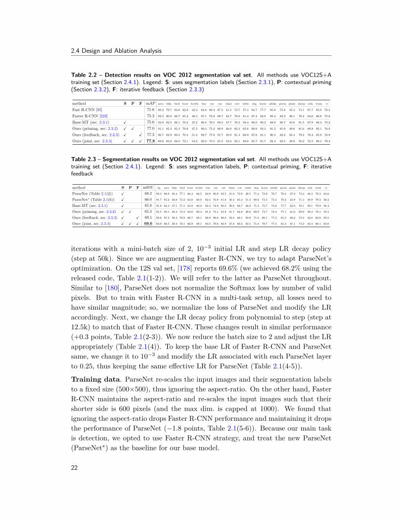
1) [178] (Original ParseNet) 500×500 10−8 1 poly 8 20k N 69.62) Reproducing [178]‡ (ParseNet) 500×500 10−8 1 poly 8 20k N 68.23) Faster R-CNN LR-policy, Norm. Loss 500×500 10−3 1 step 8 20k Y 68.54) Faster R-CNN batch-size, new LR 500×500 2.5×10⁻⁴ 1 step 2 80k Y 67.85) Faster R-CNN Base-LR 500×500 10−3 0.25 step 2 80k Y 67.86) Faster R-CNN input dim. (ParseNet∗) [600×1000]† 10−3 0.25 step 2 80k Y 66
†min dim. is 600, max dim. capped at 1000.‡https://github.com/weiliu89/caffe/tree/fcn
2.4 Design and Ablation AnalysisWe conduct experiments to better understand the impact of contextual priming anditerative feedback; and provide ablation analysis of various design decisions. Ourimplementation uses the Caffe [135] library.
2.4.1 Experimental setupFor ablation studies, we use the multi-task setup from Section 2.3.1 as our
baseline (Base-MT). We also compare our method to Faster R-CNN [223] andParseNet [178] frameworks. For quantitative evaluation, we use the standard meanaverage precision (mAP) [72] metric for object detection and mean intersection-over-union metric (mIOU) [72, 95] for segmentation.
Datasets. All models in this Section are trained on the PASCAL VOC12 [72]segmentation set (12S), augmented with the extra annotations (A) from [113] asis standard practice. Results are analyzed on VOC12 segmentation val set. Foranalysis, we chose the segmentation set, and not detection, because all images haveboth segmentation and bounding-box annotations; this helps us isolate the effects ofusing segmentation as top-down semantic feedback without worrying about missingsegmentation labels in the standard detection split. Results on the standard splitswill be presented in Section 2.5.
2.4.2 Base Model – Augmenting Faster R-CNN with SegmentationFaster R-CNN and ParseNet both use mini-batch SGD for training, however,
they follow different training methodologies. We first describe the implementationdetails and design decisions adopted to augment the segmentation module to FasterR-CNN and report baseline performances.
ParseNet Optimization. ParseNet is trained for 20k SGD iterations using aneffective mini-batch of 8 images, an initial learning rate (LR) of 10−8 and polynomialLR decay policy. Compare this to Faster R-CNN, which is trained for 70k SGD
iterations with a mini-batch size of 2, 10−3 initial LR and step LR decay policy(step at 50k). Since we are augmenting Faster R-CNN, we try to adapt ParseNet’soptimization. On the 12S val set, [178] reports 69.6% (we achieved 68.2% using thereleased code, Table 2.1(1-2)). We will refer to the latter as ParseNet throughout.Similar to [180], ParseNet does not normalize the Softmax loss by number of validpixels. But to train with Faster R-CNN in a multi-task setup, all losses need tohave similar magnitude; so, we normalize the loss of ParseNet and modify the LRaccordingly. Next, we change the LR decay policy from polynomial to step (step at12.5k) to match that of Faster R-CNN. These changes result in similar performance(+0.3 points, Table 2.1(2-3)). We now reduce the batch size to 2 and adjust the LRappropriately (Table 2.1(4)). To keep the base LR of Faster R-CNN and ParseNetsame, we change it to 10−3 and modify the LR associated with each ParseNet layerto 0.25, thus keeping the same effective LR for ParseNet (Table 2.1(4-5)).
Training data. ParseNet re-scales the input images and their segmentation labelsto a fixed size (500×500), thus ignoring the aspect-ratio. On the other hand, FasterR-CNN maintains the aspect-ratio and re-scales the input images such that theirshorter side is 600 pixels (and the max dim. is capped at 1000). We found thatignoring the aspect-ratio drops Faster R-CNN performance and maintaining it dropsthe performance of ParseNet (−1.8 points, Table 2.1(5-6)). Because our main taskis detection, we opted to use Faster R-CNN strategy, and treat the new ParseNet(ParseNet∗) as the baseline for our base model.
22
2.4 Design and Ablation Analysis
Table 2.4 – Ablation analysis of Contextual Priming and Iterative Feedback on VOC 12S val set. Allmethods use VOC 12S+A train set for training. (left) Evaluating Priming different layers; (right)Evaluating Iterative Feedback design decisions
mAP mIOU
Base-MT 75.6 65.8
Priming conv5_1 76.6 65.8Priming conv5_1, each fc6 77.0 65.3
Stage-2 Init. mAP mIOU
Base-MT - 75.6 65.8
Iterative Feedback to conv1_1ImageNet 76.5 69.3Stage-1 76.3 69.3
Iterative Feedback to conv{1,2,3,4}_1ImageNet 76.3 69.1Stage-1 77.3 69.5
Base Model Optimization. Following the changes mentioned above, our basemodel uses these standardized parameters: batch size of 2, 10−3 base LR, stepdecay policy (step at 50k), LR of 0.25 for segmentation and shared conv layers, and80k SGD iterations. This model serves as our multi-task baseline (Base-MT).
Baselines. For comparison, we re-train Fast [95] and Faster R-CNN [223] on VOC12S+A training set. We use ‘approximate joint training’ for Faster R-CNN, sameas our method [223]. Results of the Base-MT model for detection and segmentationare reported in Table 2.2 and 2.3 respectively. Performance increases by 0.3 mAPon detection and drops by 0.1 mIOU on segmentation. These results show that justadding another task for training does not effect either modules by much. This willbe our primary baseline, on top of which we will add contextual and feedback.
2.4.3 Contextual Priming
We evaluate the effects of using segmentation as top-down semantic feedbackto the region proposal generation and object detection modules. We follow thesame optimization hyperparameters as the Base-MT model, and report the resultsin Table 2.2 and 2.3. Table 2.2 shows that providing top-down feedback via primingto the Faster R-CNN modules improves its detection performance by 1.4 points overthe Base-MT model and 1.7 points over Faster R-CNN. Results in Table 2.3 showthat performance of segmentation drops slightly when it is used for priming.
Design Evaluation. In Table 2.4(left), we report the impact of providing seg-mentation signal to different modules. We see that just priming conv5_1 gives a 1
point boost over Bast-MT and adding the segmentation signal to each individualregion (‘seg+pool5’ to fc6) gives another 0.4 points boost. It is interesting thatthe segmentation performance is not affected when priming conv5_1, but it dropsby 0.5 mIOU when we prime each region. Our hypothesis is that gradients accu-mulated from all regions in the mini-batch start overpowering the gradients from
23
2.4 Design and Ablation Analysis
Table 2.5 – Detection results on VOC 2007 detection test set. All methods are trained on union ofVOC07 trainval and VOC12 trainval
method S mAP aero bike bird boat bottle bus car cat chair cow table dog horse mbike persn plant sheep sofa train tv
segmentation. To deal with this, methods like [193] can be used in the future.
2.4.4 Iterative FeedbackNext we study the impact of giving iterative top-down semantic feedback to
the entire network. In this 2-unit setup, the first unit (Stage-1) is a trained Base-MT model and the second unit (Stage-2) is a Stage-1 initialized Base-MT model(new filters are initialized randomly, see Section 2.4.4). During inference, we havethe option of using the outputs from both units or just the Stage-2 unit. Giventhat segmentation is used as feedback, it is supposed to self-improve across units,therefore we use the Stage-2 output as our final output (similar to [33, 170]). Fordetection, we combine the outputs from both units; because the Stage-2 unit ismodulated by segmentation, and the first unit is not, hence both might focus ondifferent regions.
This iterative feedback improves the segmentation performance (Table 2.3) by3.7 points over Base-MT (3.5 points over ParseNet∗). For detection, it improvesover the Base-MT model by 1.7 points (2 points over Faster R-CNN) (Table 2.2).
Design Evaluation. We study the impact of: (1) varying the degree of feedback tothe Stage-2 unit, and (2) different Stage-2 initializations. In Table 2.4(right), we seethat when initializing the Stage-2 unit with an ImageNet trained network, varyingiterative feedback does not have much impact; however, when initializing with aStage-1 model, providing more feedback leads to better performance. Specifically,iterative feedback to all shared conv layers improves both detection and segmenta-
tion by 1.7 mAP and 3.7 mIOU respectively, as opposed to feedback to just conv1_1(as in [33, 170]) which results in lower gains (Table 2.4,right). Our hypothesis isthat iterative feedback to a Stage-1 initialized unit allows the network to correct itsmistakes and/or refine its predictions; therefore, providing more feedback leads tobetter performance.
2.4.5 Joint ModelFinally, we evaluate our joint 2-unit model, where each unit is a model with
contextual priming, and both units are connected via segmentation feedback. Inthis setup, a trained contextual priming model is used as the Stage-1 unit as well asthe initialization for the Stage-2 unit. We remove the dropout layers from Stage-2unit. Inference follows the procedure described in Section 2.4.4.
As shown in Table 2.2, for detection, the joint model achieves 77.8% mAP(+2.2 points over Base-MT and +2.5 points over Faster R-CNN), which is betterthan both priming only and feedback only models. This suggests that both formsof top-down feedback are complementary for object detection. The segmentationperformance (Table 2.3) is similar to the feedback only model, which is expectedsince in both cases, the segmentation module receives similar feedback.
2.5 ResultsWe now report results on the PASCAL VOC and MS COCO [175] datasets. Wealso evaluate the region proposal generation on the proxy metric of average recall.
Experimental Setup. When training on the VOC datasets with extra data (Ta-ble 2.5, 2.6 and 2.7), we use 100k SGD iterations (other hyperparameters followSection 2.4); and for MS COCO, we use 490k SGD iterations with an initial LR of10−3 and decay step size of 200k, owing to a larger epoch size.
VOC07 and VOC12 Results. Table 2.5 shows that on VOC07, our joint prim-ing and feedback model improves the detection mAP by 1.7 points over Base-MTand 3.2 points over Faster R-CNN. Similarly, on VOC12 (Table 2.6), priming andfeedback lead to 1.5 points boost over Bast-MT (2.2 over Faster R-CNN). For
Figure 2.4 – Recall-to-IoU on VOC12 Segmentation val set (left) and VOC07 test set (right) (bestviewed digitally).
Table 2.8 – Detection results on MS COCO 2015 test-dev set. All methods use COCO trainval35kfor training and results were obtained from the online 2015 test-dev server. Legend: F: using iterativefeedback, P: using contextual priming, S: uses segmentation labels
Method S P FAP, IoU: AP, Area: AR, # Dets: AR, Area:
segmentation on VOC12 (Table 2.7), we see a huge 5 point boost in mIOU overBase-MT. We would like highlight that both Base-MT and our joint model use ex-actly the same annotations and hyperparameters; therefore the performance boostsare because of contextual priming and iterative feedback in our model.
Recall-to-IOU. Since our hypothesis is that priming and feedback lead to betterproposal generation, we also evaluate the recall of region proposals by the RPNmodule from various models, at different IOU thresholds. In Figure 2.4, we showthe results of using 2000 proposal per RPN module. Since feedback models have2 units, we report their number with both 4000 and top 2000 proposals (sorted bycls score). As can be seen priming, feedback and joint models all lead to higheraverage recall (shown in legend) over the baseline RPN module.
MS COCO Results. We also perform additional analysis of contextual primingon the COCO [175] dataset and report AP (averaged over classes, recall, and IoUlevels) in Table 2.8. Our priming model results in +1.2 AP points (+2.1 AP50)over Faster R-CNN and +0.8 AP points (+1.1 AP50) over Base-MT on the COCOtest-dev set [175]. On further analysis, we notice that the most performance gainsare for objects where context should intuitively help; e.g., +12.4 for ‘parking-meter’,+8.7 for ‘suitcase’, +8.3 for ‘umbrella’ etc. on AP50 wrt. to Faster R-CNN. Finally,our joint model achieves 27.5 AP points (+3 AP points over Faster R-CNN and
26
2.5 Results
+2.5 over Base-MT), further highlighting effectiveness of the proposed method.
Conclusion. We presented and investigated how we can incorporate top-downsemantic feedback in the state-of-the-art Faster R-CNN framework. We proposedto augment a segmentation network to Faster R-CNN, which is then used to providetop-down contextual feedback to the region proposal generation and object detectionmodules. We also use this segmentation network to provide top-down feedback to theentire Faster R-CNN network iteratively. Our results demonstrate the effectivenessof these top-down feedback mechanisms for the tasks of region proposal generation,object detection and semantic segmentation.
27
Chapter 3
Top-Down Modulation
Details are confusing. It is only by selection, by elimination,by emphasis, that we get at the real meaning of things.
Georgia O’Keeffe
Figure 3.1 – Detecting objects such as the bottle or remote shown above requires low-level finer detailsas well as high-level contextual information. In this Chapter, we propose a top-down modulation (TDM)network, which can be used with any bottom-up, feedforward ConvNet. We show that the featureslearnt by our approach lead to significantly improved object detection.
As we saw in the previous Chapter, ConvNet representations have revolutionizedthe field of object detection [16, 93, 95, 96, 223, 253, 270]. Most of these ConvNetsare bottom-up, feedforward architectures constructed using repeated convolutionallayers (with non-linearities) and pooling operations [119, 155, 258, 271, 272]. Theseconvolutional layers learn invariances and the spatial pooling increases the receptivefield of subsequent layers; thus resulting in a coarse, highly semantic representationat the final layer.
However, consider the images shown in Figure 3.1. Detecting and recognizing
29
3. Top-Down Modulation
an object like the bottle in the left image or remote in the right image requiresextraction of very fine details such as the vertical and horizontal parallel edges. Butthese are exactly the type of edges ConvNets try to gain invariance against in earlyconvolutional layers. One can argue that ConvNets can learn not to ignore suchedges when in context of other objects like table. However, objects such as table donot emerge until very late in feed-forward architecture. So, how can we incorporatethese fine details in object detection?
A popular solution is to use variants of ‘skip’ connections [16, 75, 116, 180,242, 310], that capture these finer details from lower convolutional layers with localreceptive fields. But simply incorporating high-dimensional skip features into de-tection does not yield significant improvements due to overfitting caused by curse ofdimensionality. What we need is a selection/attention mechanism that selects therelevant features from lower convolutional layers.
We believe the answer lies in the process of top-down modulation. In thehuman visual pathway, once receptive field properties are tuned using feedfor-ward processing, top-down modulations are evoked by feedback and horizontal con-nections [154, 162]. These connections modulate representations at multiple lev-els [90, 94, 211, 317, 318] and are responsible for their selective combination [47, 128].We argue that the use of skip connections is a special case of this process, where themodulation is relegated to the final classifier, which directly tries to influence lowerlayer features and/or learn how to combine them.
In this Chapter, we propose to incorporate the top-down modulation process inthe ConvNet itself. Our approach supplements the standard bottom-up, feedforwardConvNet with a top-down network, connected using lateral connections. Theseconnections are responsible for the modulation and selection of the lower layer filters,and the top-down network handles the integration of features.
Specifically, after a bottom-up ConvNet pass, the final high-level semantic fea-tures are transmitted back by the top-down network. Bottom-up features at inter-mediate depths, after lateral processing, are combined with the top-down features,and this combination is further transmitted down by the top-down network. Capac-ity of the new representation is determined by lateral and top-down connections, andoptionally, the top-down connections can increase the spatial resolution of features.These final, possibly high-res, top-down features inherently have a combination oflocal and larger receptive fields.
The proposed Top-Down Modulation (TDM) network is trained end-to-endand can be readily applied to any base ConvNet architecture (e.g., VGG [258],ResNet [119], Inception-Resnet [272] etc.). To demonstrate its effectiveness, we use
30
3.1 Related Work
T2 T3,2 T4,3
C1 C4 C5C3
T5,4
L4L3L2
ROI Classifier
ROI Proposal
Object Detector
C2I
Ci Bottom-up Blocks
Ti,j Top-down Modules
Li Lateral Modules
Forward Pass
Backprop
300 x 500 x k1600x1000x3 150 x 250 x k2
75x125 xk3 75x125 xk4
37x63xk5
75x125xa475x125 xa3
150 x 250 x a2
Described in Figure 3
Bottom-up Path
Top-down Path
Lateral P
ath
out
Figure 3.2 – The illustration shows an example of Top-Down Modulation (TDM) Network, which isintegrated with the bottom-up network with lateral connections. Ci are bottom-up, feedforward featureblocks, Li are the lateral modules which transform low level features for the top-down contextualpathway. Finally, Tj,i, which represent flow of top-down information from index j to i. Individualcomponents are explained in Figure 3.3 and 3.4.
the proposed network in the standard Faster R-CNN detection method [223] andevaluate on the challenging COCO benchmark [175]. We report a consistent andsignificant boost in performance on all metrics across network architectures. TDMnetwork increases the performance of vanilla Faster R-CNN with: (a) VGG16 from23.3 AP to 28.6 AP, (b) ResNet101 from 31.5 AP to 35.2 AP, and (c) InceptionRes-Netv2 from 34.7 AP to 37.2 AP. These are the best performances reported to-datefor these architectures without any bells and whistles (e.g., multi-scale features, it-erative box-refinement). Furthermore, we see drastic improvements in small objects(e.g., +4.5 AP) and in objects where selection of fine details using top-down contextis important.
Apart from how the architecture is designed, a difference from the previousChapter is that in TDM, we do not rely of semantic segmentation of an image toact as a proxy that provides this top-down contextual feedback.
3.1 Related WorkAfter the resurgence of ConvNets for image classification [58, 155], they have beensuccessfully adopted for a variety of computer vision tasks such as object detec-tion [95, 96, 223, 270], semantic segmentation [12, 39, 178, 180], instance segmen-tation [115, 116, 212], pose estimation [279, 285], depth estimation [67, 299], edgedetection [310], optical flow predictions [84, 220] etc. However, by construction, fi-nal ConvNet features lack the finer details that are captured by lower convolutionallayers. These finer details are considered necessary for a variety of recognition tasks,such as accurate object localization and segmentation.
31
3.1 Related Work
To counter this, ‘skip’ connections have been widely used with ConvNets. Thoughthe specifics of methods vary widely, the underlying principle is same: using or com-bining finer features from lower layers and coarse semantic features for higher layers.For example, [16, 75, 116, 242] combine features from multiple layers for the finalclassifier; while [16, 242] use subsampled features from finer scales, [75, 116] upsam-ple the features to the finest scale and use their combination. Instead of combiningfeatures, [178, 180, 310] do independent predictions at multiple layers and averagethe results. In our proposed framework, such upsampling, subsampling and fusionoperations can be easily controlled by the lateral and top-down connections.
The proposed TDM network is conceptually similar to the strategies exploredin other contemporary works [12, 176, 213, 220, 226]. All methods, including ours,propose architectures that go beyond the standard skip-connection paradigm and/orfollow a coarse-to-fine strategy when using features from multiple levels of thebottom-up feature hierarchy. However, different methods focus on different taskswhich guide their architectural design and training methodology.
Conv-deconv [198] and encoder-decoder style networks [12, 226] have been usedfor image segmentation to utilize finer features via lateral connections. These con-nections generally use the ‘unpool’ operation [319], which merely inverts the spatialpooling operation. Moreover, there is no modulation of bottom-up network. In com-parison, our formulation is more generic and is responsible for the flow of high-levelcontext features [211].
Pinheiro et al. [213] focus on refining class-agnostic object proposals by firstselecting proposals purely based on bottom-up feedforward features [212], and thenpost-hoc learning how to refine each proposal independently using top-down and lat-eral connections (due to the computational complexity, only a few proposals can beselected to be refined). We argue that this use of top-down and lateral connectionsfor refinement is sub-optimal for detection because it relies on the proposals selectedbased on feedforward features, which are insufficient to represent small and difficultobjects. This training methodology also limits the ability to update the feedforwardnetwork through lateral connections. In contrast to this, we propose to learn betterfeatures for recognition tasks in an end-to-end trained system, and these featuresare used for both proposal generation and object detection. Similar to the idea ofcoarse-to-fine refinement, Ranjan and Black [220] propose a coarse-to-fine spatialpyramid network, which computes a low resolution residual optical flow and itera-tively improves predictions with finer pyramid levels. This is akin to only using aspecialized top-down network, which is suited for low-level tasks (like optical flow)but not for recognition tasks. Moreover, such purely coarse-to-fine networks cannot
32
3.2 Top-Down Modulation (TDM)
utilize models pre-trained on large-scale datasets [58], which is important for recog-nition tasks [96]. Therefore, our approach learns representation using bottom-up(fine-to-coarse), top-down (coarse-to-fine) and lateral networks simultaneously, andcan use different pre-trained modules.
The proposed top-down network is closest to the recent work of Lin et al. [176],developed concurrently to ours, on feature pyramid network for object detection.Lin et al. [176] use bottom-up, top-down and lateral connections to learn a featurepyramid, and require multiple proposal generators and region classifiers on eachlevel of the pyramid. In comparison, the proposed top-down modulation focuses onusing these connections to learn a single final feature map that is used by a singleproposal generator and region classifier.
There is strong evidence of such top-down context, feedback and lateral pro-cessing in the human visual pathway [47, 90, 94, 128, 154, 161, 162, 211, 317,318]; wherein, the top-down signals are responsible for modulating low-level fea-tures [90, 94, 211, 317, 318] as well as act as attentional mechanism for selectionof features [47, 128]. In this Chapter, we propose a computation model that cap-tures some of these intuitions and incorporates them in a standard ConvNets, givingsubstantial performance improvements.
Our top-down framework is also related to the process of contextual feed-back [11]. To incorporate top-down feedback loop in ConvNets, contemporaryworks [33, 89, 170, 250], have used ‘unrolled’ networks (trained stage-wise). Evenin Chapter 6, we used semantic segmentation as a proxy for top-down feedback.The proposed top-down network with lateral connections explores a complemen-tary paradigm and can be readily combined with them. Contextual features havealso been used for ConvNets based object detectors; e.g., using other objects [110]or regions [98] as context. We believe the proposed top-down path can naturallytransmit these contextual features.
3.2 Top-Down Modulation (TDM)Our goal is to incorporate top-down modulation into current object detection frame-works. The key idea is to select/attend to fine details from lower level featuremaps based on top-down contextual features and select top-down contextual fea-tures based on the fine low-level details. We formalize this by proposing a simpletop-down modulation (TDM) network as shown in Figure 3.2.
The TDM network starts from the last layer of bottom-up feedforward net-work. For example, in the case of VGG16, the input to the first layer of the TDM
33
3.2 Top-Down Modulation (TDM)
CiH x W x ki
xiC
H x W x li
xiL
Li
Tj,i H x W x tj
xjT
2H x 2Wx ti
xiT
Figure 3.3 – The basic building blocks of Top-Down Modulation Network (detailed Section 3.2.1).
network is the conv5_3 output. Every layer of TDM network also gets the bottom-up features as inputs via lateral connections. Thus, the TDM network learns to:(a) transmit high-level contextual features that guide the learning and selection ofrelevant low-level features, and (b) use the bottom-up features to select the contex-tual information to transmit. The output of the proposed network captures bothpertinent finer details and high-level information.
3.2.1 Proposed Architecture
An overview of the proposed framework is illustrated in Figure 3.2. The stan-dard bottom-up network is represented by blocks of layers, where each block Ci hasmultiple operations. The TDM network hinges on two key components: a lateralmodule L, and a top-down module T (see Figure 3.3). Each lateral module Li takesin a bottom-up feature xC
i (output of Ci) and produces the corresponding lateralfeature xL
i . These lateral features xLi and top-down features xT
j are combined, andoptionally upsampled, by the Tj,i module to produce the top-down features xT
i .These modules, Tj,i and Li, control the capacity of the modulation network bychanging their output feature dimensions.
The feature from the last top-down module Touti is used for the task of object
detection. For example, in Figure 3.2, instead of xC5 , we use Tout
2 as input to ROIproposal and ROI classifier networks of the Faster R-CNN [223] detection system(discussed in Section 3.3.1). During training, gradient updates from the object detec-tor backpropagate via top-down and lateral modules to the Ci blocks. The lateralmodules L• learn how to transform low-level features and the top-down modulesT• learn what semantic or context information to preserve in the top-down featuretransmission as well as the selection of relevant low-level lateral features. Ultimately,the bottom-up features are modulated to adapt for this new representation.
34
3.2 Top-Down Modulation (TDM)
T3,2
2x
L23x3
Conv
1x1
Conv
T2
250l2
150
t3,2
Bottom-up Feature150 x 250 x k2
Top-downFeature
75 x 125 x t4,3150 x 250 x tout
OutputFeature
3x3
Conv
out
Figure 3.4 – An example with details of top-down modules and lateral connections. Please see Sec-tion 3.2.1 for details of the architecture.
Architecture details. The top-down and lateral modules described above areessentially small ConvNets, which can vary from a single or a hierarchy of convo-lutional layers to more involved blocks with Residual [119] or Inception [272] units.In this Chapter, we limit our study by using modules with a single convolutionallayer and non-linearity to analyze the impact of top-down modulation.
A detailed example of lateral and top-down modules is illustrated in Figure 3.4.The lateral module Li is a 3× 3 convolutional layer with ReLU non-linearity, whichtransforms an (Hi × Wi × ki) input xC
i , to (Hi × Wi × li) lateral feature xLi . The top-
down module Tj,i is also a 3× 3 convolutional layer with ReLU, that combines thislateral feature with (Hi × Wi × tj) top-down feature xT
j , to produce an intermediateoutput (Hi × Wi × ti). If the resolution of next lateral feature xL
i−1 is higher than theprevious lateral feature (e.g., Hi−1 = 2× Hi), then Tj,i also upsamples the interme-diate output to produce (Hi−1 × Wi−1 × ti) top-down feature xT
i . In Figure 3.2, wedenote ai = tj + li for simplicity. The final Tout
i module can additionally have a1 × 1 convolutional layer with ReLU to output a (Hi × Wi × kout) feature, which isused by the detection system.
Varying li, ti and kout controls the capacity of the top-down modulation systemand dimension of the output features. These hyperparameters are governed bythe base network design, detection system and hardware constraints (discussed inSection 3.3.3). Notice that the upsampling step is optional and depends on thecontent and arrangement of C blocks (e.g., no upsampling by T4 in Figure 3.2).Also, the first top-down module (T5 in the illustration) only operates on xC
5 (thefinal output of the bottom-up network).
Training methodology. Integrating top-down modulation framework into a bottom-up ConvNet is only meaningful when the latter can represent high-level concepts inhigher layers. Thus, we typically start with a pre-trained bottom-up network (see
35
3.3 Approach Details
Table 3.1 – Base networks architecture details for VGG16, ResNet101 and InceptionResNetv2. Legend:Ci: bottom-up block id, N: number of convolutional filters, NR: number of residual units, NI: numberof inception-resnet units, dim
(xCi
): Resolution and dimensions of the output feature. Refer to [119,
Section 3.5.4 for discussion). Starting with this pre-trained network, we find thatprogressively building the top-down network performs better in general. Therefore,we add one new pair of lateral and top-down modules at a time. For example, forthe illustration in Figure 3.2, we will begin by adding (L4,T5,4) and use Tout
4 toget features for object detection. After training (L4,T5,4) modules, we will add thenext pair (L3,T4,3) and use a new Tout
3 module to get features for detection; andwe will repeat this process. With each new pair, the entire network, top-down andbottom-up along with lateral connections, is trained end-to-end. Implementationdetails of this training methodology depends on the base network architecture, andwill be discussed in Section 3.3.3.
To better understand the impact of the proposed TDM network, we conductextensive experimental evaluation; and provide ablation analysis of various designdecisions. We describe our approach in detail (including preliminaries and imple-mentation details) in Section 3.3 and present our results in Section 3.4. We alsoreport ablation analysis in Section 3.5. We would like to highlight that the proposedframework leads to substantial performance gains across different base network ar-chitectures, indicating its wide applicability.
3.3 Approach DetailsIn this Section, we describe the preliminaries and provide implementation details ofour top-down modulation (TDM) network under various settings. We first give a abrief overview of the object detection system and the ConvNet architectures usedthroughout this Chapter.
3.3.1 Preliminaries: Faster R-CNNWe use the Faster R-CNN [223] framework as our base object detection system
(we only recap relevant terminology here; please refer to Section 2.2 for details).Faster R-CNN consists of two core modules: 1) ROI Proposal Network (RPN),
36
3.3 Approach Details
which takes an image as input and proposes rectangular regions of interests (ROIs);and 2) ROI Classifier Network (RCN), which is a Fast R-CNN [95] detector thatclassifies these proposed regions and learns to refine ROI coordinates. Given animage, Faster R-CNN first uses a ConvNet to extract features that are shared byboth RPN and RCN. RPN uses these features to propose candidate ROIs, which arethen classified by RCN. The RCN network projects each ROI onto the shared featuremap and performs the ‘ROI Pooling’ [95, 120] operation to extract a fixed lengthrepresentation. Finally, this feature is used for classification and box regression.See [95, 120, 129, 223] for details.
Due to lack of support for recent ConvNet architectures [119, 272] in the FasterR-CNN framework, we use our implementation in Tensorflow [1]. We follow thedesign choices outlined in [129]. In Section 3.4, we will provide performance numbersusing both the released code [223] as well as our implementation (which tends togenerally perform better). We use the end-to-end training paradigm for Faster R-CNN for all experiments [223]. Unless specified otherwise, all methods start withmodels that were pre-trained on ImageNet classification [58, 96].
3.3.2 Preliminaries: Base Network Architectures
In this Chapter, we use three standard ConvNet architectures: VGG16 [258],ResNet101 [119] and InceptionResNetv2 [272]. We briefly explain how they areincorporated in the Faster R-CNN framework (see [119, 129, 223] for details), andgive a quick overview of these architectures with reference to the bottom-up blocksC from Section 3.2.1.
We use the term ‘Base Network’ to refer to the part of ConvNet that is sharedby both RPN and RCN; and ‘Classifier Network’ to refer to the part that is usedas RCN. For VGG16 [223, 258], ConvNet till conv5_3 is used as the base network,and the following two fc layers are used as the classifier network. Similarly, forResNet101 [119, 223], base network is the ConvNet till conv4_x, and classifier net-work is the conv5_x block (with 3 residual units or 9 convolutional layers). ForInceptionResNet101v2 [129, 272], ConvNet till the ‘Block_20x’ is used as the basenetwork, and the remaining layers (‘Mixed_7a’ and ‘Block_9x’, with a total of11 inception-resnet units or 48 convolutional layers) are used as the classifier net-work. Following [129], we change the pooling stride of the penultimate convolutionalblock in ResNet101 and InceptionResNetv2 to 1 to maintain spatial resolution, anduse atrous [39, 178] convolution to recover the original field-of-view. Properties ofbottom-up blocks Ci, including number of layers, the output feature resolution andfeature dimension etc. are given in Table 3.1.
37
3.3 Approach Details
Table 3.2 – Top-Down Modulation network design for VGG16, ResNet101 and InceptionResNetv2.Notice that tout VGG16 is much smaller than 512, thus requiring fewer parameters in RPN and RCNmodules. Also note that it is important to keep tout fixed for ResNet101 and InceptionResNetv2 in orderto utilize pre-trained RPN and RCN modules
Table 3.3 – Object detection results on the COCO benchmark. Different methods use different networksfor region proposal generation (ROINet) and for region classification (ClsNet). Results for the topblock (except Faster R-CNN⋆) were directly obtained from their respective publications [119, 213, 223,250]. Faster R-CNN⋆ was reproduced by us. Middle block shows our implementation of Faster R-CNNframework, which is our primary baseline. Bottom block presents the main results of TDM network,with the state-of-the-art single-model performance (when [254] was published) highlighted
Method train test ROINet ClsNet AP AP50 AP75 APS APM APL AR1 AR10 AR100 ARS ARM ARL
To add the proposed TDM network to the ConvNet architectures describedabove, we need to decide the extent of top-down modulation, the frequency of lateralconnections and the capacity of T, L and Tout modules. We try to follow theseprinciples when making design decisions: (a) coarse semantic modules need largercapacity; (b) lateral and top-down connections should reduce feature dimensionalityin order to force selection; and (c) the capacity of Tout should be informed bythe Proposal (RPN) and Classifier (RCN) Network design. Finally, the hardwareconstraint that a TDM augmented ConvNet should fit on a standard GPU.
To build a TDM network, we start with a standard bottom-up model trainedon the detection task, and add (Ti,j ,Lj) progressively. The capacity for differentT, L, and Tout modules is given in Table 3.2. For the VGG16 network, we add top-down and lateral modules all the way to the conv1_x feature. Notice that the input
38
3.4 Results
feature dimension to RPN and RCN networks changes from 512 (for conv5_x) to256 (for Tout
4 ), therefore we initialize the fc layers in RPN and RCN randomly [100].However, since tout is same for the last three Tout modules, we re-use the RPN andRCN layers for these modules.
For the ResNet101 and InceptionResNetv2, we add top-down and lateral mod-ules for till conv1 and ‘Mixed_5b’ respectively. Similar to VGG16, their basenetworks are initialized with a model pre-trained on the detection task. However,as opposed to VGG16, where the RCN has just 2 fc layers, ResNet101 and Incep-tionResNetv2 models have an RCN with 9 and 48 convolutional layers respectively.This makes training RCN from random initialization difficult. To counter this, weensure that all Tout output feature dimensions (tout) are same, so that we can bereadily use pre-trained RPN and RCN. This is implemented using an additional1× 1 convolutional layer wherever (ti,j + lj) differs from tout (e.g., all Tout modulesin ResNet101, and the final Tout module in InceptionResNetv2).
We would like to highlight an issue with training of RPN at high-resolutionfeature maps. RPN is a fully convolutional module of Faster R-CNN, that generatesan intermediate 512 dimension representation which is of the same resolution asinput; and losses are computed at all pixel locations. This is efficient for coarsefeatures (e.g., last row in Table 3.1), but the training becomes prohibitively slowfor finer resolution features. To counter this, we apply RPN at a stride whichensures that computation remains exactly the same (e.g., using stride of 8 for Tout
1 inVGG16). Because of ‘ROI Pooling’ operations, RCN module still efficiently utilizesthe finer resolution features.
3.4 Results
In this Section, we evaluate our method on the task of object detection, and demon-strate consistent and significant improvement in performance when using featuresfrom the proposed TDM network.
Dataset and metrics. All experiments and analysis in this Chapter are per-formed on the COCO dataset [175]. All models were trained on 40k train and 32kval images (which we refer to as ‘trainval∗’ set). All ablation evaluations were per-formed on 8k val images (‘minival∗’ set) held out from the val set. We also reportquantitative results on the standard testdev2015 split. For quantitative evaluation,we use the AP averaged over classes, recall, and IoU levels.
39
3.4 Results
Experimental Setup. We conduct experiments with three standard ConvNetarchitectures: VGG16 [258], ResNet101 [119] and InceptionResNetv2 [272]. Allmodels (‘Baseline’ Faster R-CNN and ours) were trained with SGD for 1.5M mini-batch iterations, with batch size of 256 and 128 ROIs for RPN and RCN respectively.We start with an initial learning rate of 0.001 and decay it by 0.1 at 800k and 900kiterations.
Baselines. Our primary baseline is using vanilla VGG16, ResNet101 and Incep-tionResNetv2 features in the Faster R-CNN framework. However, due to lack ofimplementations supporting all three ConvNets, we opted to re-implement FasterR-CNN in Tensorflow [1]. The baseline numbers reported in Table 3.3(middle) areusing our implementation and training schedule and are generally higher than theones reported in [223, 250]. Faster R-CNN⋆ was reproduced by us using the officialimplementation [223]. All other results in Table 3.3(top) were obtained from theoriginal papers.
We also compare against models which use a single region proposal genera-tor and a single region classifier network. In particular, we compare with Sharp-Mask [213], because of its refinement modules with top-down and lateral connec-tions, and [250] because they also augment the standard VGG16 network with top-down information. Note that different methods use different networks and train/testsplits (see Table 3.3), making it difficult to do a comprehensive comparison. There-fore, for discussion, we will directly compare against our Faster R-CNN baseline(Table 3.3(middle)), and highlight that the improvements obtained by our approachare much bigger than the boosts by other methods.
3.4.1 COCO ResultsIn Table 3.3(bottom), we report results of the proposed TDM network on the
testdev2015 split of the COCO dataset. We see that the TDM network leads toa 5.3 AP point boost over the vanilla VGG16 network (28.6 AP vs. 23.3 AP),indicating that TDM learns much better features for object detection. Note thateven though our algorithm is trained on less data (trainval∗), we outperform allmethods with VGG16 architecture. For ResNet101, we improve the performance by3.7 points to 35.2 AP. InceptionResNetv2 [272] architecture was the cornerstone ofthe winning entry to COCO 2016 detection challenge [129]. The best single modelperformance used by this entry achieves 34.7 AP on the testdev split ([129]). UsingInceptionResNetv2 as base, our TDM network achieves 37.3 AP, which is currentlythe state-of-the-art single model performance on the testdev split without anybells and whistles (e.g., multi-scale, iterative box refinement, etc.). In fact, the
40
3.4 Results
TDM network outperforms the baselines (with same base networks) on almost allAP and AR metrics. Similarly, in Table 3.5, we observe that TDM achieves similarboosts across all network architectures on the minival∗ split as well.
Figure 3.5 shows change in AP from Faster R-CNN baseline to the TDM net-work (for the testdev split). When using VGG16, for all but one category, TDMfeatures improve the performance on object detection. In fact, more than 50% ofthe categories improve by 5 AP points or more, highlighting that the features aregood for small and big objects alike. Similar trends hold for ResNet101 and Incep-tionResNetv2.
In Table 3.4, we report AP results on the COCO testdev split for all classes.Results are reported for baseline Faster R-CNN and our TDM network with differ-ent base network architectures. The proposed TDM network results in substantialimprovement in AP across all network architectures and object categories. In partic-ular, we see significant improvements for small objects and on stricter AP75 metric.
Improved localization. In Table 3.3, we also notice that for VGG16, our methodperforms exceptionally well on the AP75 metric, improving the baseline Faster R-CNN by 8.9 AP75 points, which is much higher than the 3.5 point AP50 boost. Webelieve that using contextual features to select and integrate low-level finer detailsis they key reason for this improvement. Similarly for ResNet101 and InceptionRes-Netv2, we see 4.8 AP75 and 3.1 AP75 boost respectively.
Improvement for small objects. In Table 3.3, for VGG16, ResNet101 and In-ceptionResNetv2), we see 4.8, 3 and 3.6 point boost respectively for small objects(APS) highlighting the effectiveness of features with TDM. Moreover, small objectsare often on top of the list in Figure 3.5 (e.g., sportsball +13 AP point, mouse +10AP for VGG16). This is in line with other studies [110], which show that contextis particularly helpful for some objects. Similar trends hold for the minival∗ splitas well: 5.6, 7.4 and 8.5 APS boost for VGG16, ResNet101 and InceptionRes-Netv2 respectively. Also refer to Table 3.4 for per-category results for all networkarchitectures.
Qualitative Results. In Figure 3.6, we display qualitative results of the Top-down Modulation Network. Notice that the network can find small objects likeremote (second row, last column; fourth row, first column) and sportsball (secondrow, third and fourth column). Also notice the detection results in the presence ofheavy clutter.
41
3.4 Results
0 5 10 15
Change in AP →
hairdrierbookcake
toothbrushhotdog
appleorangespoon
bananacarrot
handbagbaseballbat
broccoliknife
scissorsbackpack
bearsuitcase
boatbench
sinkparkingmeter
pottedplantcellphone
toasterdogskis
firehydrantumbrella
diningtablechair
surfboardbed
sandwichovenbird
baseballglovesnowboard
vasemicrowave
cattv
pizzatennisracket
donuttie
bowllaptopbicycle
truckfork
teddybearremotecouchtoilet
keyboardmotorcycle
cupbottle
personskateboard
clockstopsign
frisbeeairplane
wineglasshorse
trafficlightsheep
giraffetraincowcar
refrigeratorelephant
kitezebra
mousebus
sportsball
VGG16
−4 0 4 8
Change in AP →
toasterhairdriercellphone
beardog
orangebanana
benchteddybear
birdpottedplant
bookbroccoli
cakehotdog
sandwichboat
parkingmeterdonutapple
catbackpack
ovenbed
toilethandbag
carrottoothbrush
clockbowltrain
airplaneremote
truckchairvase
zebragiraffehorse
bicyclemotorcycle
scissorssinkbus
spoonmicrowave
sheepdiningtable
skisumbrella
tvperson
tennisracketknifepizza
cupcar
bottlecowtie
mouserefrigerator
surfboardtrafficlight
elephantfrisbee
firehydrantwineglass
laptopsuitcase
skateboardfork
stopsignkeyboard
baseballglovesportsball
couchsnowboardbaseballbat
kite
ResNet101
−4 0 4 8
Change in AP →
hairdriertoaster
toiletcat
broccolisandwich
appletrain
teddybeardog
pizzamicrowave
bearbench
refrigeratorcake
orangetv
horsebananascissorsgiraffe
firehydrantcarrotlaptop
cellphonemotorcycle
busbackpack
bookspoon
hotdogovenbed
snowboardumbrella
toothbrushcouchchair
elephantdonut
vasepottedplantdiningtable
bowlzebraboatsink
parkingmetersurfboard
mousekeyboard
frisbeehandbag
birdskateboard
bicycleairplane
baseballbatclock
suitcasestopsign
trucktie
knifetennisracket
cowperson
cupskis
baseballglovetrafficlight
bottlefork
sheepkite
remotewineglass
carsportsball
InceptionResNetv2
Figure 3.5 – Improvement in AP over Faster R-CNN baseline. Base Networks: (left) VGG16, (middle)ResNet101, and (right) InceptionResNetv2. Improved performance for almost all categories emphasizethe effectiveness of Top-Down Modulation for object detection. (best viewed digitally)
42
3.4 Results
Figure 3.6 – Qualitative results of the proposed TDM network on randomly selected images from theminival∗ set (best viewed digitally).
43
3.4 Results
Table 3.4 – COCO testdev detection AP results for all classes using different network architectures.Results are reported for baseline Faster R-CNN (B) and our method (+TDM). All methods use trainval∗for training
Network → VGG16 Resnet101 InceptionResNetB +TDM B +TDM B +TDM
Table 3.5 – Ablation analysis on the COCO benchmark using the Faster R-CNN detection framework.All methods are trained on trainval∗ and evaluated on minival∗ set (Section 3.4). Methods are groupedbased on their base network, best results are highlighted in each group.
Method Net Featuresfrom: AP AP50 AP75 APS APM APL AR1 AR10 AR100 ARS ARM ARL
3.5 Design and Ablation AnalysisIn this Section, we perform control and ablative experiments to study the importanceof top-down and lateral modules in the proposed TDM network.
3.5.1 How low should the Top-Down Modulation go?In Section 3.3.3, we discussed the principles that we follow to add top-down and
lateral modules. We connected these modules till the lowest layer choosing designdecisions that hardware constraints would permit. However, is that overkill? Isthere an optimal layer, after which this modulation does not help or starts hurting?To answer these questions, we limit the layer till which the modulation processhappens, and use those features for Faster R-CNN.
Recall that the TDN network is built progressively, i.e., we add one pair oflateral and top-down module at a time. So for this control study, we simply leteach subsequent pair train for the entire learning schedule, treating the Tout as thefinal output. We report the results on minival∗ set in Table 3.5. As we can see,adding more top-down modulation helps in general. However, for VGG16, we seethat the performance saturates at Tout
2 , and adding modules till Tout1 do not seem to
help much. Deciding the endpoint criteria for top-down modulation is an interestingfuture direction.
3.5.2 No lateral modulesTo analyze the importance of lateral modules, and to control for the extra pa-
rameters added by the TDM network (Table 3.2), we train additional baselines with
45
3.5 Design and Ablation Analysis
Table 3.6 – Importance of lateral modules. (top block) ∼ Ti,j is a modified top-down module toaccount for more parameters in the TDM network. (bottom block) (Ti,j ,Lj) is the proposed top-downmodulation network. All methods use the VGG16 network
with L AP AP50 AP75 APS APM APL AR1 AR10 AR100 ARS ARM ARL
variants of VGG16 + TDM network. In particular, we remove the lateral modulesand use convolutional and upsampling operations from the top-down modules T totrain ‘deeper’ variants of VGG16 as baseline. To control for the extra parametersfrom lateral modules, we also increase the parameters in the convolutional layers.Note that for this baseline, we follow training methodology and design decisionsused for training TDM networks.
As shown in Table 3.6, even though using more depth increases the performanceslightly, the performance boost due to lateral modules is much higher. This high-lights the importance of dividing the capacity of TDM network amongst lateral andtop-down modules.
3.5.3 No top-down modules
Next we want to study the importance of the top-down path introduced by ourTDM network. We believe that this path is responsible for transmitting contextualfeatures and for selection of relevant finer details. Removing the top-down pathexposes the ‘skip’-connections from bottom-up features, which can be used for objectdetection. We follow the strategy from [16], where they ROI-pool features fromdifferent layers, L2-normalize and concatenate these features and finally scale themback to the original conv5_3 magnitude and dimension.
We tried many variants of the Skip-pooling baseline, and report the best resultsin Table 3.5 (Skip-pool). We see that performance for small objects (APS) increasesslightly, but overall the AP does not change much. This highlights the importanceof using high-level contextual features in the top-down path for the selection oflow-level features.
46
3.5 Design and Ablation Analysis
Table 3.7 – Impact of Pre-training. All methods use Resnet101 as the base network
pre-trainedon: AP AP50 AP75 APS APM APL AR1 AR10 AR100 ARS ARM ARL
3.5.4 Impact of Pre-trainingFinally, we study the impact of using a model pre-trained on the detection
task to initialize our base networks and ResNet101/InceptionResNetv2’s RPN andRCN networks vs. using only an image classification [58] pre-trained model. InTable 3.7, we see that initialization does not impact the performance by a hugemargin. However, pre-training on the detection task is consistently better thanusing the classification initialization.
Conclusion. This Chapter introduces the Top-Down Modulation (TDM) net-work, which leverages top-down contextual features and lateral connections to bottom-up features for object detection. The TDM network uses top-down context to selectlow-level finer details, and learns to integrate them together. Through extensiveexperiments on the challenging COCO dataset, we demonstrate the effectivenessand importance of features from the TDM network. We show empirically that theproposed representation benefits all objects, big and small, and is helpful for accu-rate localization. Even though we focused on the object detection, we believe thesetop-down modulated features will be helpful in a wide variety of computer visiontasks.
47
Chapter 4
Online Hard Example Mining
If you would only recognize that life is hard,things would be so much easier for you.
Louis Brandeis
The Object detection systems, including the ones discussed in the last twoChapters, are trained through a reduction that converts object detection into animage classification problem. This reduction introduces a new challenge that isnot found in natural image classification tasks: the training set is distinguishedby a large imbalance between the number of annotated objects and the number ofbackground examples (image regions not belonging to any object class of interest).In the case of sliding-window object detectors, such as the deformable parts model(DPM) [79], this imbalance may be as extreme as 100,000 background examples toevery one object. The recent trend towards object-proposal-based detectors [96, 288]mitigates this issue to an extent, but the imbalance ratio may still be high (e.g.,70:1). This challenge opens space for learning techniques that cope with imbalanceand yield faster training, higher accuracy, or both.
Unsurprisingly, this is not a new challenge and a standard solution, originallycalled bootstrapping (and now often called hard negative mining), has existed for atleast 20 years. Bootstrapping was introduced in the work of Sung and Poggio [268]in the mid-1990’s (if not earlier) for training face detection models. Their key ideawas to gradually grow, or bootstrap, the set of background examples by selectingthose examples for which the detector triggers a false alarm. This strategy leadsto an iterative training algorithm that alternates between updating the detectionmodel given the current set of examples, and then using the updated model to findnew false positives to add to the bootstrapped training set. The process typicallycommences with a training set consisting of all object examples and a small, random
49
4. Online Hard Example Mining
set of background examples.
Bootstrapping has seen widespread use in the intervening decades of objectdetection research. Dalal and Triggs [54] used it when training SVMs for pedes-trian detection. Felzenszwalb et al. [79] later proved that a form of bootstrappingfor SVMs converges to the global optimal solution defined on the entire dataset.Their algorithm is often referred to as hard negative mining and is frequently usedwhen training SVMs for object detection [96, 120, 288]. Bootstrapping was alsosuccessfully applied to a variety of other learning models, including shallow neu-ral networks [230] and boosted decision trees [62]. Even modern detection methodsbased on deep convolutional neural networks (ConvNets) [155, 166], such as R-CNN[96] and sppnet [120], still employ SVMs trained with hard negative mining.
It may seem odd then that the current state-of-the-art object detectors, embod-ied by Fast R-CNN [95] and its descendants [223], do not use bootstrapping. Theunderlying reason is a technical difficulty brought on by the shift towards purelyonline learning algorithms, particularly in the context of deep ConvNets trainedwith stochastic gradient descent (SGD) on millions of examples. Bootstrapping,and its variants in the literature, rely on the aforementioned alternation template:(a) for some period of time a fixed model is used to find new examples to add tothe active training set; (b) then, for some period of time the model is trained onthe fixed active training set. Training deep ConvNet detectors with SGD typicallyrequires hundreds of thousands of SGD steps and freezing the model for even a fewiterations at a time would dramatically slow progress. What is needed, instead, isa purely online form of hard example selection.
In this Chapter, we propose a novel bootstrapping technique called online hardexample mining1 (OHEM) for training state-of-the-art detection models based ondeep ConvNets. The algorithm is a simple modification to SGD in which trainingexamples are sampled according to a non-uniform, non-stationary distribution thatdepends on the current loss of each example under consideration. The methodtakes advantage of detection-specific problem structure in which each SGD mini-batch consists of only one or two images, but thousands of candidate examples. Thecandidate examples are subsampled according to a distribution that favors diverse,high loss instances. Gradient computation (backpropagation) is still efficient becauseit only uses a small subset of all candidates. We apply OHEM to the standard FastR-CNN detection method and show three benefits compared to the baseline trainingalgorithm:
1We use the term hard example mining, rather than hard negative mining, because our methodis applied in a multi-class setting to all classes, not just a “negative” class.
50
4.1 Related Work
• It removes the need for several heuristics and hyperparameters commonly usedin region-based ConvNets.
• It yields a consistent and significant boosts in mean average precision.
• Its effectiveness increases as the training set becomes larger and more difficult,as demonstrated by results on the MS COCO dataset.
Moreover, the gains from OHEM are complementary to recent improvementsin object detection, such as multi-scale testing [120] and iterative bounding-boxregression [93]. Combined with these tricks, OHEM gives state-of-the-art results of78.9% and 76.3% mAP on PASCAL VOC 2007 and 2012, respectively.
4.1 Related WorkObject detection is one of the oldest and most fundamental problems in computervision. The idea of dataset bootstrapping [230, 268], typically called hard negativemining in recent work [79], appears in the training of most successful object detec-tors [54, 62, 79, 93, 96, 120, 185, 230, 260]. Many of these approaches use SVMs asthe detection scoring function, even after training a deep convolutional neural net-work (ConvNet) [155, 166] for feature extraction. One notable exception is the FastR-CNN detector [95] and its descendants, such as Faster R-CNN [223]. Since thesemodels do not use SVMs, and are trained purely online with SGD, existing hard ex-ample mining techniques cannot be immediately applied. This work addresses thatproblem by introducing an online hard example mining algorithm that improves op-timization and detection accuracy. We briefly review hard example mining, modernConvNet-based object detection, and relationships to concurrent works using hardexample selection for training deep networks.
Hard example mining. There are two hard example mining algorithms in com-mon use. The first is used when optimizing SVMs. In this case, the training al-gorithm maintains a working set of examples and alternates between training anSVM to convergence on the working set, and updating the working set by removingsome examples and adding others according to a specific rule [79]. The rule removesexamples that are “easy” in the sense that they are correctly classified beyond thecurrent model’s margin. Conversely, the rule adds new examples that are hard inthe sense that they violate the current model’s margin. Applying this rule leads tothe global SVM solution. Importantly, the working set is usually a small subset ofthe entire training set.
The second method is used for non-SVMs and has been applied to a variety of
51
4.2 Preliminaries: Fast R-CNN
models including shallow neural networks [230] and boosted decision trees [62]. Thisalgorithm usually starts with a dataset of positive examples and a random set ofnegative examples. The machine learning model is then trained to convergence onthat dataset and subsequently applied to a larger dataset to harvest false positives.The false positives are then added to the training set and then the model is trainedagain. This process is usually iterated only once and does not have any convergenceproofs.
ConvNet-based object detection. In the last three years significant gains havebeen made in object detection. These improvements were made possible by thesuccessful application of deep ConvNets [155] to ImageNet classification [58]. TheR-CNN [96] and OverFeat [243] detectors lead this wave with impressive resultson PASCAL VOC [72] and ImageNet detection. OverFeat is based on the sliding-window detection method, which is perhaps the most intuitive and oldest searchmethod for detection. R-CNN, in contrast, uses region proposals [4, 7, 32, 43, 69,153, 288, 329], a method that was made popular by the selective search algorithm[288]. Since R-CNN, there has been rapid progress in region-based ConvNets, in-cluding sppnet [120], MR-CNN [93], and Fast R-CNN [95], which our work buildson.
Hard example selection in deep learning. There is recent work [181, 257, 297]concurrent to our own that selects hard examples for training deep networks. Similarto our approach, all these methods base their selection on the current loss for eachdatapoint. [257] independently selects hard positive and negative example froma larger set of random examples based on their loss to learn image descriptors.Given a positive pair of patches, [297] finds hard negative patches from a large setusing triplet loss. Akin to our approach, [181] investigates online selection of hardexamples for mini-batch SGD methods. Their selection is also based on loss, butthe focus is on ConvNets for image classification. Complementary to [181], we focuson online hard example selection strategy for region-based object detectors.
4.2 Preliminaries: Fast R-CNNWe first summarize the Fast R-CNN [95] (FRCN) framework. FRCN takes as inputan image and a set of object proposal regions of interest (RoIs). The FRCN networkitself can be divided into two sequential parts: a convolutional (conv) network withseveral convolution and max-pooling layers (Figure 4.1, “Convolutional Network”);and an RoI network with an RoI-pooling layer, several fully-connected (fc) layersand two loss layers (Figure 4.1, “RoI Network”).
52
4.2 Preliminaries: Fast R-CNN
Convolution Feature Maps
Last Conv.
Feature Map
Mini-batch Sampler
Selective-Search RoIs (R)
|R| ≈ 2000|Rsel| = Batch Size
Rsel𝑖
RoI Pooling Layer
FullyConnected
Layers
SoftmaxClassification
Loss
Soft-L1Bbox Reg.
Loss
For each R𝐬𝐞𝐥
Convolutional Network RoI Network
Figure 4.1 – Architecture of the Fast R-CNN approach (see Section 4.2 for details).
During inference, the conv network is applied to the given image to producea conv feature map, size of which depends on the input image dimensions. Then,for each object proposal, the RoI-pooling layer projects the proposal onto the convfeature map and extracts a fixed-length feature vector. Each feature vector is fed intothe fc layers, which finally give two outputs: (1) a softmax probability distributionover the object classes and background; and (2) regressed coordinates for bounding-box relocalization.
There are several reasons for choosing FRCN as our base object detector, apartfrom it being a fast end-to-end system. Firstly, the basic two network setup (convand RoI) is also used by other recent detectors like sppnet and MR-CNN; therefore,our proposed algorithm is more broadly applicable. Secondly, though the basic setupis similar, FRCN also allows for training the entire conv network, as opposed to bothsppnet and MR-CNN which keep the conv network fixed. And finally, both sppnetand MR-CNN require features from the RoI network to be cached for training aseparate SVM classifier (using hard negative mining). FRCN uses the RoI networkitself to train the desired classifiers. In fact, [95] shows that in the unified systemusing the SVM classifiers at later stages was unnecessary.
4.2.1 Training
Like most deep networks, FRCN is trained using stochastic gradient descent(SGD). The loss per example RoI is the sum of a classification log loss that encour-ages predicting the correct object (or background) label and a localization loss thatencourages predicting an accurate bounding box (see [95] for details).
To share conv network computation between RoIs, SGD mini-batches are cre-ated hierarchically. For each mini-batch, N images are first sampled from thedataset, and then B/N RoIs are sampled from each image. Setting N = 2 andB = 128 works well in practice [95]. The RoI sampling procedure uses severalheuristics, which we describe briefly below. One contribution of this Chapter is to
53
4.3 Our Approach
eliminate some of these heuristics and their hyperparameters.
Foreground RoIs. For an example RoI to be labeled as foreground (fg), itsintersection over union (IoU) overlap with a ground-truth bounding box should beat least 0.5. This is a fairly standard design choice, in part inspired by the evaluationprotocol of the PASCAL VOC object detection benchmark. The same criterion isused in the SVM hard mining procedures of R-CNN, sppnet, and MR-CNN. We usethe same setting.
Background RoIs. A region is labeled background (bg) if its maximum IoU withground truth is in the interval [bg_lo, 0.5). A lower threshold of bg_lo = 0.1 is usedby both FRCN and sppnet, and is hypothesized in [95] to crudely approximate hardnegative mining; the assumption is that regions with some overlap with the groundtruth are more likely to be the confusing or hard ones. We show in Section 4.4.4 thatalthough this heuristic helps convergence and detection accuracy, it is suboptimalbecause it ignores some infrequent, but important, difficult background regions. Ourmethod removes the bg_lo threshold.
Balancing fg-bg RoIs: To handle the data imbalance described in the beginningof this Chapter, [95] designed heuristics to rebalance the foreground-to-backgroundratio in each mini-batch to a target of 1 : 3 by undersampling the background patchesat random, thus ensuring that 25% of a mini-batch is fg RoIs. We found that thisis an important design decision for the training FRCN. Removing this ratio (i.e.randomly sampling RoIs), or increasing it, decreases accuracy by ∼3 points mAP.With our proposed method, we can remove this ratio hyperparameter with no illeffect.
4.3 Our ApproachWe propose a simple yet effective online hard example mining algorithm for trainingFast R-CNN (or any Fast R-CNN style object detector). We argue that the currentway of creating mini-batches for SGD (Section 4.2.1) is inefficient and suboptimal,and we demonstrate that our approach leads to better training (lower training loss)and higher testing performance (mAP).
4.3.1 Online Hard Example MiningRecall the alternating steps that define a hard example mining algorithm: (a)
for some period of time a fixed model is used to find new examples to add to the
54
4.3 Our Approach
Convolution Feature Maps
Selective-Search RoIs (R)
|R| ≈ 2000
|Rhard−sel| = Batch Size
Last Conv.
Feature Map
Rhard−sel𝑖
RoI Pooling Layer
FullyConnected
Layers
Each R𝑖
FullyConnected
Layers
For each RRead-only Layer
Order of Computation:1. Forward for Conv. Network
2. Forward for each R𝑖 ( )3. Selection of Rhard−sel
4. Forward-Backward for each Rhard−sel𝑖 ( )
5. Backward for Conv. Network
Backward Computation for:
1. Each Rhard−sel𝑖 ( )
2. Gradient Accumulation by RoI Pooling Layer
3. Conv. Network ( )
Convolutional Network RoI Network
Shared Weights
Forward for each R𝑖
Forward-Backward each R𝑖
Forward-Backward for each Image
(b)
(a)
SoftmaxClassification
Loss
Soft-L1Bbox Reg.
Loss
SoftmaxClassification
Loss
Soft-L1Bbox Reg. Loss
∑
Diverse & Hard RoI Sampler
For each Rhard−sel
Figure 4.2 – Architecture of the proposed training algorithm. Given an image, and selective searchRoIs, the conv network computes a conv feature map. In (a), the readonly RoI network runs a forwardpass on the feature map and all RoIs (shown in green arrows). Then the Hard RoI module uses theseRoI losses to select B examples. In (b), these hard examples are used by the RoI network to computeforward and backward passes (shown in red arrows).
active training set; (b) then, for some period of time the model is trained on thefixed active training set. In the context of SVM-based object detectors, such as theSVMs trained in R-CNN or sppnet, step (a) inspects a variable number of images(often 10’s or 100’s) until the active training set reaches a threshold size, and thenin step (b) the SVM is trained to convergence on the active training set. Thisprocess repeats until the active training set contains all support vectors. Applyingan analogous strategy to FRCN ConvNet training slows learning because no modelupdates are made while selecting examples from the 10’s or 100’s of images.
Our main observation is that these alternating steps can be combined with howFRCN is trained using online SGD. The key is that although each SGD iterationsamples only a small number of images, each image contains thousands of exampleRoIs from which we can select the hard examples rather than a heuristically sampledsubset. This strategy fits the alternation template to SGD by “freezing” the modelfor only one mini-batch. Thus the model is updated exactly as frequently as withthe baseline SGD approach and therefore learning is not delayed.
More specifically, the online hard example mining algorithm (OHEM) proceedsas follows. For an input image at SGD iteration t, we first compute a conv featuremap using the conv network. Then the RoI network uses this feature map and the allthe input RoIs (R), instead of a sampled mini-batch [95], to do a forward pass. Recallthat this step only involves RoI pooling, a few fc layers, and loss computation for each
55
4.3 Our Approach
RoI. The loss represents how well the current network performs on each RoI. Hardexamples are selected by sorting the input RoIs by loss and taking the B/N examplesfor which the current network performs worst. Most of the forward computation isshared between RoIs via the conv feature map, so the extra computation needed toforward all RoIs is relatively small. Moreover, because only a small number of RoIsare selected for updating the model, the backward pass is no more expensive thanbefore.
However, there is a small caveat: co-located RoIs with high overlap are likelyto have correlated losses. Moreover, these overlapping RoIs can project onto thesame region in the conv feature map, because of resolution disparity, thus lead-ing to loss double counting. To deal with these redundant and correlated regions,we use standard non-maximum suppression (NMS) to perform deduplication (theimplementation from [95]). Given a list of RoIs and their losses, NMS works byiteratively selecting the RoI with the highest loss, and then removing all lower lossRoIs that have high overlap with the selected region. We use a relaxed IoU thresholdof 0.7 to suppress only highly overlapping RoIs.
We note that the procedure described above does not need a fg-bg ratio fordata balancing. If any class were neglected, its loss would increase until it has ahigh probability of being sampled. There can be images where the fg RoIs are easy(e.g. canonical view of a car), so the network is free to use only bg regions in amini-batch; and vice-versa when bg is trivial (e.g. sky, grass etc.), the mini-batchcan be entirely fg regions.
4.3.2 Implementation details
There are many ways to implement OHEM in the FRCN detector, each withdifferent trade-offs. An obvious way is to modify the loss layers to do the hardexample selection. The loss layer can compute loss for all RoIs, sort them basedon this loss to select hard RoIs, and finally set the loss of all non-hard RoIs to 0.Though straightforward, this implementation is inefficient as the RoI network stillallocates memory and performs backward pass for all RoIs, even though most RoIshave 0 loss and hence no gradient updates (a limitation of current deep learningtoolboxes).
To overcome this, we propose the architecture presented in Figure 4.2. Ourimplementation maintains two copies of the RoI network, one of which is readonly.This implies that the readonly RoI network (Figure 4.2(a)) allocates memory onlyfor forward pass of all RoIs as opposed to the standard RoI network, which allocatesmemory for both forward and backward passes. For an SGD iteration, given the
56
4.4 Design and Ablation Analysis
Table 4.1 – Impact of hyperparameters on FRCN training
conv feature map, the readonly RoI network performs a forward pass and computesloss for all input RoIs (R) (Figure 4.2, green arrows). Then the hard RoI sam-pling module uses the procedure described in Section 4.3.1 to select hard examples(Rhard-sel), which are input to the regular RoI network (Figure 4.2(b), red arrows)).This network computes forward and backward passes only for Rhard-sel, accumulatesthe gradients and passes them to the conv network. In practice, we use all RoIs fromall N images as R, therefore the effective batch size for the readonly RoI networkis |R| and for the regular RoI network is the standard B from Section 4.2.1.
We implement both options described above using the Caffe [135] framework(see [95]). Our implementation uses gradient accumulation withN forward-backwardpasses of single image mini-batches. Following FRCN [95], we use N = 2 (whichresults in |R| ≈ 4000) and B = 128. Under these settings, the proposed architecture(Figure 4.2) has similar memory footprint as the first option, but is > 2× faster.Unless specified otherwise, the architecture and settings described above will beused throughout this Chapter.
4.4 Design and Ablation Analysis
This Section compares FRCN training with online hard example mining (OHEM)to the baseline heuristic sampling approach. We also compare FRCN with OHEMto a less efficient approach that uses all available example RoIs in each mini-batch,not just the B hardest examples.
57
4.4 Design and Ablation Analysis
4.4.1 Experimental SetupWe conduct experiments with two standard ConvNet architectures: VGG_CNN_M_1024
(VGGM, for short) from [36], which is a wider version of alexnet [155], and VGG16from [258]. All experiments in this Section are performed on the PASCAL VOC07dataset. Training is done on the trainval set and testing on the test set. Unlessspecified otherwise, we will use the default settings from FRCN [95]. We train allmethods with SGD for 80k mini-batch iterations, with an initial learning rate of0.001 and we decay the learning rate by 0.1 every 30k iterations. The baseline num-bers reported in Table 4.1 (row 1-2) were reproduced using our training scheduleand are slightly higher than the ones reported in [95].
4.4.2 OHEM vs. Heuristic SamplingStandard FRCN, reported in Table 4.1 (rows 1 − 2), uses bg_lo = 0.1 as a
heuristic for hard mining (Section 4.2.1). To test the importance of this heuristic,we ran FRCN with bg_lo = 0. Table 4.1 (rows 3 − 4) shows that for VGGM,mAP drops by 2.4 points, whereas for VGG16 it remains roughly the same. Nowcompare this to training FRCN with OHEM (rows 11−13). OHEM improves mAPby 2.4 points compared to FRCN with the bg_lo = 0.1 heuristic for VGGM, and 4.8
points without the heuristic. This result demonstrates the sub-optimality of theseheuristics and the effectiveness of our hard mining approach.
4.4.3 Robust Gradient EstimatesOne concern over using only N = 2 images per batch is that it may cause
unstable gradients and slow convergence because RoIs from an image may be highlycorrelated [273]. FRCN [95] reports that this was not a practical issue for theirtraining. But this detail might raise concerns over our training procedure becausewe use examples with high loss from the same image and as a result they may bemore highly correlated. To address this concern, we experiment with N = 1 in orderto increase correlation in an effort to break our method. As seen in Table 4.1 (rows5 − 6, 11), performance of the original FRCN drops by ∼1 point with N = 1, butwhen using our training procedure, mAP remains approximately the same. Thisshows that OHEM is robust in case one needs fewer images per batch in order toreduce GPU memory usage.
4.4.4 Why just hard examples, when you can use all?Online hard example mining is based on the hypothesis that it is important to
consider all RoIs in an image and then select hard examples for training. But what if
Figure 4.3 – Training loss is computed for various training procedures using VGG16 networks discussedin Section 4.4. We report mean loss per RoI. These results indicate that using hard mining for trainingleads to lower training loss than any of the other heuristics.
we train with all the RoIs, not just the hard ones? The easy examples will have lowloss, and won’t contribute much to the gradient; training will automatically focuson the hard examples. To compare this option, we ran standard FRCN trainingwith a large mini-batch size of B = 2048, using bg_lo = 0, N ∈ {1, 2} and withother hyperparameters fixed. Because this experiment uses a large mini-batch, it’simportant to tune the learning rate to adjust for this change. We found optimalresults by increasing it to 0.003 for VGG16 and 0.004 for VGGM. The outcomes arereported in Table 4.1 (rows 7− 10). Using these settings, mAP of both VGG16 andVGGM increased by ∼1 point compared to B = 128, but the improvement fromour approach is still > 1 points over using all RoIs. Moreover, because we computegradients with a smaller mini-batch size training is faster.
4.4.5 Better OptimizationFinally, we analyze the training loss for the various FRCN training methods
discussed above. It’s important to measure training loss in a way that does notdepend on the sampling procedure and thus results in a valid comparison betweenmethods. To achieve this goal, we take model snapshots from each method every 20ksteps of optimization and run them over the entire VOC07 trainval set to computethe average loss over all RoIs. This measures the training set loss in a way thatdoes not depend on the example sampling scheme.
Figure 4.3 shows the average loss per RoI for VGG16 with the various hyperpa-rameter settings discussed above and presented in Table 4.1. We see that bg_lo = 0
results in the highest training loss, while using the heuristic bg_lo = 0.1 results in a
59
4.5 Results
Table 4.2 – Computational statistics of training FRCN [95] and FRCN with OHEM (using an NvidiaTitan X GPU)
VGGM VGG16
FRCN Ours FRCN FRCN* Ours*
time (sec/iter) 0.13 0.22 0.60 0.57 1.00max. memory (G) 2.6 3.6 11.2 6.4 8.7*: uses gradient accumulation over two forward/backward passes
much lower training loss. Increasing the mini-batch size to B = 2048 and increasingthe learning rate lowers the training loss below the bg_lo = 0.1 heuristic. Ourproposed online hard example mining method achieves the lowest training loss ofall methods, validating our claims that OHEM leads to better training for FRCN.
4.4.6 Computational CostOHEM adds reasonable computational and memory overhead, as reported in
Table 4.2. OHEM costs 0.09s per training iteration for VGGM network (0.43s forVGG16) and requires 1G more memory (2.3G for VGG16). Given that FRCN [95] isa fast detector to train, the increase in training time is acceptable for most scenarios.
4.5 ResultsIn this Section, we evaluate our method on VOC 2012 [72] as well as the morechallenging MS COCO [175] dataset. We demonstrate consistent and significantimprovement in FRCN performance when using the proposed OHEM approach.Per-class results are also presented on VOC 2007 for comparison with prior work.
Experimental Setup. We use VGG16 for all experiments. When training onVOC07 trainval, we use the SGD parameters as in Section 4.4 and when using extradata (07+12 and 07++12, see Table 4.3 and 4.4), we use 200k mini-batch iterations,with an initial learning rate of 0.001 and decay step size of 40k. When training onMS COCO [175], we use 240k mini-batch iterations, with an initial learning rate of0.001 and decay step size of 160k, owing to a larger epoch size.
4.5.1 VOC 2007 and 2012 ResultsTable 4.3 shows that on VOC07, OHEM improves the mAP of FRCN from
67.2% to 69.9% (and 70.0% to 74.6% with extra data). On VOC12, OHEM leads toan improvement of 4.1 points in mAP (from 65.7% to 69.8%). With extra data, weachieve an mAP of 71.9% as compared to 68.4% mAP of FRCN, an improvement
60
4.6 Adding Bells and Whistles
Table 4.3 – VOC 2007 test detection average precision (%). All methods use VGG16. Trainingset key: 07: VOC07 trainval, 07+12: union of 07 and VOC12 trainval. All methods use bounding-box regression. Legend: M: using multi-scale for training and testing, B: multi-stage bbox regression.FRCN⋆ refers to FRCN [95] with our training schedule
method M B train set mAP aero bike bird boat bottle bus car cat chair cow table dog horse mbike persn plant sheep sofa train tv
of 3.5 points. Interestingly the improvements are not uniform across categories.Bottle, chair, and tvmonitor show larger improvements that are consistent acrossthe different PASCAL splits. Why these classes benefit the most is an interestingand open question.
4.5.2 MS COCO Results
To test the benefit of using OHEM on a larger and more challenging dataset,we conduct experiments on MS COCO [175] and report numbers from test-dev 2015evaluation server (Table 4.5). On the standard COCO evaluation metric, FRCN [95]scores 19.7% AP, and OHEM improves it to 22.6% AP.2 Using the VOC overlapmetric of IoU ≥ 0.5, OHEM gives a 6.6 points boost in AP50. It is also interestingto note that OHEM helps improve the AP of medium sized objects by 4.9 pointson the strict COCO AP evaluation metric, which indicates that the proposed hardexample mining approach is helpful when dealing with smaller sized objects. Notethat FRCN with and without OHEM were trained on MS COCO train set.
4.6 Adding Bells and WhistlesWe’ve demonstrated consistent gains in detection accuracy by applying OHEM toFRCN training. In this Section, we show that these improvements are orthogonalto recent bells and whistles that enhance object detection accuracy. OHEM withthe following two additions yields state-of-the-art results on VOC and competitiveresults on MS COCO.
2COCO AP averages over classes, recall, and IoU levels. See http://mscoco.org/dataset/#detections-eval for details.
Table 4.4 – VOC 2012 test detection average precision (%). All methods use VGG16. Trainingset key: 12: VOC12 trainval, 07++12: union of VOC07 trainval, VOC07 test, and VOC12 trainval,+COCO: a model trained on COCO trainval and fine-tuned on 07++12. Legend: M: using multi-scalefor training and testing, B: iterative bbox regression
method M B train set mAP aero bike bird boat bottle bus car cat chair cow table dog horse mbike persn plant sheep sofa train tv
Multi-scale (M). We adopt the multi-scale strategy from sppnet [120] (andused by both FRCN [95] and MR-CNN [93]). Scale is defined as the size of theshortest side (s) of an image. During training, one scale is chosen at random,whereas at test time inference is run on all scales. For VGG16 networks, we uses ∈ {480, 576, 688, 864, 900} for training, and s ∈ {480, 576, 688, 864, 1000} duringtesting, with the max dimension capped at 1000. The scales and caps were chosenbecause of GPU memory constraints.
Iterative bounding-box regression (B). We adopt the iterative localizationand bounding-box (bbox) voting scheme from [93]. The network evaluates eachproposal RoI to get scores and relocalized boxes R1. High-scoring R1 boxes are therescored and relocalized, yielding boxes R2. Union of R1 and R2 is used as the finalset RF for post-processing, where RNMS
F is obtained using NMS on RF with an IoUthreshold of 0.3 and weighted voting is performed on each box ri in RNMS
F usingboxes in RF with an IoU of ≥0.5 with ri (see [93] for details).
4.6.1 VOC 2007 and 2012 ResultsWe report the results on VOC benchmarks in Table 4.3 and 4.4. On VOC07,
FRCN with the above mentioned additions achieves 72.4% mAP and OHEM im-proves it to 75.1%, which is currently the highest reported score under this setting(07 data). When using extra data (07+12), OHEM achieves 78.9% mAP, surpass-ing the current state-of-the-art MR-CNN (78.2% mAP). We note that MR-CNNuses selective search and edge boxes during training, whereas we only use selectivesearch boxes. Our multi-scale implementation is also different, using fewer scalesthan MR-CNN. On VOC12 (Table 4.4), we consistently perform better than MR-CNN. When using extra data, we achieve state-of-the-art mAP of 76.3% (vs. 73.9%mAP of MR-CNN).
Ablation Analysis. We now study in detail the impact of these two additionsand whether OHEM is complementary to them, and report the analysis in Table 4.6.Baseline FRCN mAP improves from 67.2% to 68.6% when using multi-scale duringboth training and testing (we refer to this as M). However, note that there is only amarginal benefit of using it at training time. Iterative bbox regression (B) furtherimproves the FRCN mAP to 72.4%. But more importantly, using OHEM improvesit to 75.1% mAP, which is state-of-the-art for methods trained on VOC07 data (seeTable 4.3). In fact, using OHEM consistently results in higher mAP for all variantsof these two additions (see Table 4.6).
4.6.2 MS COCO ResultsMS COCO [175] test-dev 2015 evaluation server results are reported in Table 4.5.
Using multi-scale improves the performance of our method to 24.4% AP on thestandard COCO metric and to 44.4% AP50 on the VOC metric. This again shows
63
4.6 Adding Bells and Whistles
the complementary nature of using multi-scale and OHEM. Finally, we train ourmethod using the entire MS COCO trainval set, which further improves performanceto 25.5% AP (and 45.9% AP50). In the 2015 MS COCO Detection Challenge, avariant of this approach finished 4th place overall.
Conclusion We presented an online hard example mining (OHEM) algorithm,a simple and effective method to train region-based ConvNet detectors. OHEMeliminates several heuristics and hyperparameters in common use by automaticallyselecting hard examples, thus simplifying training. We conducted extensive exper-imental analysis to demonstrate the effectiveness of the proposed algorithm, whichleads to better training convergence and consistent improvements in detection accu-racy on standard benchmarks. We also reported state-of-the-art results on PASCALVOC 2007 and 2012 when using OHEM with other orthogonal additions. Thoughwe used Fast R-CNN throughout this Chapter, OHEM can be used for training anyregion-based ConvNet detector.
Our experimental analysis was based on the overall detection accuracy, howeverit will be an interesting future direction to study the impact of various trainingmethodologies on individual category performance.
64
Chapter 5
Geometric-structure fromMulti-modal Data
You can’t criticize geometry.It’s never wrong.
Paul Rand
Input Predicted GeometryG-DPM Detections
Figure 5.1 – Examples of object detection and surface normal prediction using the proposed G-DPMmodel. Our G-DPM not only improves the state of the art performance in object detection but it alsopredicts the surface normals with the detection. Legend for normals: blue: X; green: Y; red: Z.
The standard output of an object recognition systems discussed so far is eithera box around the localized object (detection) or per-pixel labels (segmentation).Though critical building blocks for perception, these outputs offer a rather shallowunderstanding of the recognized object. For example, they have no geometric un-derstanding that augmented reality and robotics applications might need. In thisChapter, we present a system to infer 3D properties of objects from 2D images.
We propose a geometry-driven deformable part-based model (G-DPM) that
65
5.1 Related Work
can be learned from a set of labeled RGBD images. In a G-DPM, object parts aredefined based on their physical properties (i.e., their geometry) rather than justtheir appearance. Our key hypothesis is that while the arrangement of parts mightvary across the instances of object categories, the constituent parts will still haveconsistent underlying 3D geometry. For example, every sofa has a L-shaped partthat is the intersection of a vertical surface and a horizontal surface for sitting.Therefore, the underlying 3D geometry can provide weak supervision to define andinitialize the parts. While the learning objective in case of G-DPM is still non-convex(similar to [79]), we show how the depth data can be used as weak supervision toimpose geometric constraints and guide latent updates at each step. Empirically thisleads to faster convergence, and a better model in terms of detection performance.But more importantly, because our parts have a 3D geometrical representation theycan be used to jointly detect objects and infer 3D properties from a single 2D image.Figure 5.1 shows two examples of objects detected by our G-DPM model and thepredicted surface normal geometry by the G-DPM. Notice how our approach predictsnicely aligned flat horizontal surface of the table within the bounding box and howthe approach predicts the horizontal and vertical surfaces of the couch.
Contributions. Our key contributions include: (1) We propose to marry de-formable part-based model with the geometric representation of objects by definingparts based on consistent underlying 3D geometry. (2) We demonstrate how the geo-metric representation can help us leverage depth data during training and constrainthe latent model learning problem. The underlying 3D geometry during traininghelps us guide the latent steps in the right direction. (3) Most importantly, a jointgeometric and appearance based representation not only allows us to achieve state-of-the results on object detection but also allows us to tackle the grand challenge ofunderstanding 3D objects from 2D images.
5.1 Related WorkThe idea of using geometric and physical representation for objects and their cate-gories has a rich history in computer vision [27, 182, 187]. While these approachesresulted in some impressive demos such as ACRONYM [28], these systems failedto generalize. That led us to the modern era in computer vision where instead ofrepresenting objects in 3D, the focus changed to representing objects using low-levelimage features such as HOG [54] and using machine learning to learn an appearancemodel of the object. The most successful approaches in this line of work are thedeformable part-based models [79] that extend the rigid template from [54] to alatent part-based model that is trained discriminatively. While there has been a lot
66
5.1 Related Work
of progress made over the last decade, the performance of these appearance basedapproaches seems to have been stagnated.
Therefore, recent research has now focused on developing richer representationsfor objects and effective ways of learning these representations. Most of the recentwork on improving deformable part models can be broadly divided in two maincategories:
(a) Better 2D Representations and Learning: The first and the most com-mon way is to design better representations using 2D image features. In this area,researchers have looked into using strongly-supervised models for parts [10, 26, 70,313], using key point annotations to search for parts [25] or discovering mid-levelparts in a completely unsupervised manner [260]. Other directions include usingsharing to increase data-size across categories [173] or finding visual subcategoriesbased on appearances before learning a part-based model [41, 60].
(b) Using 3D Geometry: The second direction that has been explored is to bringback the flavor of the past and develop rich models by representing 3D geometryexplicitly. One of the most common ways to encode viewpoint information is totrain a mixture of templates for different viewpoints [102]. An alternative approachis to explicitly consider the 3D nature of the problem and model objects as a col-lection of local parts that are connected across views [99, 237, 263, 309]. Anotherway to account for 3D representation is to explicitly model the 3D object in termsof planes [44, 82, 237, 308] or parts [209], and use a rigid template [121], springmodel [82] or a CRF [44].
Our approach lies at the intersection of two these directions. Unlike other ap-proaches which incorporate geometry in DPM via CAD models [209] or manually-labeled 3D cuboids [82, 121], our approach uses noisy depth data for training (similarto [85]). This allows us to access more and diverse data (hundreds of images com-pared to 40 or so CAD models). The scale at which we build 3D priors and dogeometric reasoning during latent learning allows us to obtain improvements of asmuch as 11% in some categories (previous approaches performed at-par or belowDPM). We would also like to point out that even though our approach uses depthinformation during training, it is used as a weak supervisory signal (and not as anextra input feature) to guide the training in the right direction. The discriminativemodel is only learned in the appearance space. Therefore, we do not require depthat test time and can use G-DPM to detect objects in RGB images. Most other workin object detection/recognition using RGBD [21, 159, 160] uses depth as an extrainput feature to learn an object model and therefore, also requires depth informationat test time.
67
5.2 Overview
5.2 OverviewAs input to the system, at training, we use RGB images of object instances alongwith their underlying geometry in terms of depth data. We convert the depth datainto surface normals using the standard procedure from [256]. Our goal is to learna deformable part-based model where the parts are defined based on their appear-ance and underlying geometry. We argue that using a geometric representation inconjunction with appearance based deformable parts model not only allows us tohave a better initialization but also provides additional constraints during the latentupdate steps. Specifically, our learning procedure ensures not only that the latentupdates are consistent in the appearance space but also that the geometry predictedby underlying parts is consistent with the ground truth geometry. Hence, the depthdata is not used as an extra feature, but instead provides weak supervision duringthe latent update steps.
In this Chapter, we present a proof-of-concept system for building G-DPM. Welimit our focus on man-made indoor rigid objects, such as bed, sofa etc., for three rea-sons: (1) These classes are primarily defined based on their physical properties, andtherefore learning a geometric model for these categories makes intuitive sense; (2)These classes have high intra-class variation and are challenging for any deformableparts model. We would like to demonstrate that a joint geometric and appearancebased representation gives us a powerful tool to model intra-class variations; (3)Finally, due to the availability of Kinect, data collection for these categories hasbecome simpler and efficient. In our case, we use the NYU v2 dataset [256], whichhas 1449 RGBD images.
5.3 Technical ApproachGiven a large set of training object instances in the form of RGBD data, our goalis to discover a set of candidate parts based on consistent underlying geometry, anduse these parts to learn a geometry-driven deformable part-based model (G-DPM).To obtain such a set of candidate parts, we first discover a dictionary of geometricelements based on their depth information (Section 5.3.1) in a category-free manner(pooling the data from all categories). A category-free dictionary allows us to sharethe elements across multiple object categories.
We use this dictionary to choose a set of parts for every object category basedon frequency of occurrence and consistency in the relative location with respect tothe object bounding-boxes. Finally, we use these parts to initialize and learn ourG-DPM using latent updates and hard mining. We exploit the geometric nature ofour parts and use them to enforce additional geometrical constraints at the latent
68
5.3 Technical Approach
Incr
easi
ng m
in (𝜎
,𝜎)
Good Clusters
Bad Clusters
Rejected
Figure 5.2 – A few elements from the dictionary after the initialization step. They are ordered tohighlight the over-completeness of our initial dictionary.
update steps (Section 5.3.3).
5.3.1 Geometry-driven Dictionary of 3D ElementsGiven a set of labeled training images and their corresponding surface normal
data, our goal is to discover a dictionary of elements capturing 3D information thatcan act as parts in DPM. Our elements should be: 1) representative: frequent amongthe object categories in question; 2) spatially consistent with respect to the object.(e.g., a horizontal surface always occurs on the top of a table and bed, while it occursat center of a chair and a sofa). To obtain a dictionary of candidate elements whichsatisfy these properties, we use a two step process: first we initialize our dictionaryby an over-complete set of elements, each satisfying the representativeness property;and then we refine the dictionary elements based on their relative spatial locationwith respect to the object.
Initializing the dictionary. We sample hundreds of thousands of patches, in 3
different aspect-ratios (AR), from the object bounding boxes in the training images(100−500 patches per object bounding box). We represent these patches in terms oftheir raw surface normal maps. To extract a representative set of elements for eachAR, we perform clustering using simple k-means (with k ∼ 1000), in raw surfacenormal space. This clustering process leads to an over-complete set of geometricelements. We remove any cluster with less than N members, for not satisfying thefrequency property. We represent every remaining cluster by an element which is thepixel-wise median of the nearest N patches to the cluster center. A few examples ofthis set of elements is shown in Figure 5.2. In practice, we use N = 25. As one cannotice from the figure, the dictionary is over-complete. To reject the clusters with
69
5.3 Technical Approach
Increasing min (𝜎 , 𝜎 ) Good Clusters Bad Clusters
Rejected
Figure 5.3 – Refinement: After creating an initial dictionary we do the refinement procedure where wefind the set of elements that occur at a consistently occur at same spatial location with respect to theobject center.
Incr
easi
ng m
in (𝜎
,𝜎)
Good Clusters
Bad Clusters
Rejected
Figure 5.4 – A few examples of resulting elements in dictionary after the refinement procedure.
bad (non-homogenous) members and to remove redundancy we follow this clusteringstep with a refinement procedure.
Refinement. Given the clusters from the initialization step, we first check eachcluster for spatial consistency, i.e., how consistent the cluster is with respect tothe center of the object. For this, we record the location of each member in thecluster relative to the object center as: (dxi, dyi) =
((pix−pox)
wo ,(piy−poy)
ho
), where po,
wo and ho are the object center, width and height respectively, and pi is the centerof element i. Examples of this voting scheme are given in Figure 5.3, where eachblue dot represents a vote from the cluster’s member, and red dot represents objectcenter. To capture consistency in relative locations, we sort the clusters based onmin(σ2x(dx), σ2y(dy)) (minimum variance of their relative x, y locations). Clusterslike the legs of furniture (consistently below the object and closer to the center) andsides of a bed (consistently near the center of object) rank much higher than noisycluster shown at the right. After pruning bad clusters by thresholding, we performa step of agglomerative clustering to merge good clusters which are close in featurespace (raw surface normals) as well as have consistent distribution of (dx, dy). Thisgives us a dictionary D of 3D elements. A few examples of resulting elements areshown in Figure 5.4.
70
5.3 Technical Approach
Figure 5.5 – An example of detection/localization of discovered dictionary elements in surface normalspace.
5.3.2 From 3D Parts to Object Hypothesis
Given a dictionary of geometric elements D, we would like to discover whichgeometric elements can act as parts for which object categories. Since our categoriesshare the geometric elements, every element in the dictionary can act as a part forany number of object categories. We represent a part pj for an object categorywith three aspects: (a) the geometric element ei ∈ D; (b) the relative locationlj : (dxj , dyj) of the part with respect to object center (in normalized coordinates);(c) the spring model (or variance in (dx, dy)) for the part, which defines how spatiallyconsistent a part is with respect to the object. Note that an object part is differentfrom the geometric element and a geometric element can act as different parts basedon the location (e.g., two armrests for the chair; an armrest is a geometric elementbut two different parts). The goal is to find set of parts (or an object hypothesis)p =
[p1, . . . , pN
], where pj : (ei, lj), that occur consistently in the labeled images.
Similar to DPM [79], we represent each object category as a mixture of compo-nents and each component is loosely treated as a category of its own. Therefore, ourgoal is to find a set of parts for each component of all object categories. Given a setof training images for a component, we first localize each element e in the surfacenormal map. For example, Figure 5.5 shows the elements detected in the case ofa sofa. We then pool the element localizations from all images and find the mostfrequent elements at different locations in an object. These frequent elements act ascandidate parts for representing an object. Figure 5.6(b) shows the candidate partsfor one component of three categories: bed, sofa and table.
We now use a greedy approach to select the final parts with the constraints thatwe have 6-12 parts per object component and that these parts cover at least 60%of the object area. At each step, we select the top-most part hypothesis based onthe frequency of occurrence and consistency in the relative location with respect to
71
5.3 Technical Approach
(a) Sample Objects (b) Frequent Parts (c) Selected Consistent Parts
Tabl
e B
ed
Sofa
Figure 5.6 – From 3D Parts to object hypothesis: (a) few examples images in the cluster; (b) all thegeometrically consistent candidate parts selected (before greedy selection); (c) final part hypothesis forinitializing G-DPM (after greedy selection)
the object. Therefore, if a geometric element occurs quite frequently at a particularlocation, then it is selected as a part for the object. Once we have selected a part,the next part is selected based on frequency and consistency of occurrence, andits overlap with the already selected parts (a part that overlaps a lot with alreadyselected parts is rejected).
5.3.3 Learning G-DPM
Once we have obtained a set of parts for a given object category, we can now useit to initialize the learning of our proposed G-DPM model. Following the generalframework of deformable part models [10, 70, 79, 313], we model an object by amixture of M components, each of which is a non-rigid star-shaped constellation ofparts. The key difference between learning the G-DPM and the original DPM liesin the scoring function. Unlike the original model which only captures appearanceand location of parts, we explicitly include a geometric consistency term in thescoring function used at the latent update step. This allows us to enforce geometricconsistency across the latent update steps and guide the latent updates in the rightdirection. We will now first discuss a few preliminaries about DPM and then discuss
72
5.3 Technical Approach
Table gDPM Model 1 Table gDPM Model 2 Table gDPM Model 3
Bed gDPM Model 3 Bed gDPM Model 2 Bed gDPM Model 1
Sofa gDPM Model 3 Sofa gDPM Model 2 Sofa gDPM Model 1
Figure 5.7 – Learned G-DPM models for classes bed, sofa and table. The first visualization in eachtemplate represents the learned appearance root filter, the second visualization contains learned partfilters super-imposed on the root filter, the third visualization is the surface normal map correspondingto each part and the fourth visualization is of the learned deformation penalty.
how we add the geometric consistency term to the scoring function.
DPM Preliminaries. For each mixture component, indexed by c ∈ {1, . . . ,M},the object hypothesis is specified by z = (l0, l1, . . . , lnc), where li = (ui, vi, si) denotesthe (u, v)-position of i-th filter (every part acts a filter) at level si in the featurepyramid (root is indexed at 0, and l0 corresponds to its bounding-box) and nc isnumber of parts in component c. Following [79], we enforce that each part is attwice the resolution of the root.
The score of a mixture component c, with model parameter βc, at any given z(root and part locations) in an image I is given by
S(I, z, βc) =
nc∑i=0
Fi · ϕ(I, li)−nc∑i=1
di · ψ(li − l0) + b (5.1)
where the first term scores appearance using image features ϕ(I, li) (HOG fea-tures in this case) and model’s appearance parameters (F0, . . . , Fnc). The secondterm enforces the deformation penalty using ψ(li − l0) = {dx, dy, dx2, dy2} where(dx, dy) = (lxi , l
yi ) − (2(lx0 , l
y0) − vi) and vi is the anchor position of the part. Thus,
each component’s model parameter is βc = {F0, . . . , Fnc , d1, . . . , dnc , b}.The final score of a DPM model for an object category on an image I at any z
is given by
S(I, z) = maxc∈{1...M}
S(I, z, βc), (5.2)
which is the maximum over scores of all the components. Thus, the final objectmodel parameter is β = (β1, . . . , βM ) which encapsulates allM mixture components.
73
5.3 Technical Approach
Enforcing Geometric Constraints & LearningGiven the training data {(xi, yi)}1,...,N , we aim to learn a discriminative G-
DPM. In our case, x = {I, IG, l}, where I denotes an RGB image, IG denotes thesurface normal map and l is location of the bounding box, and y ∈ {−1, 1}. Similarto [10, 70, 79, 313], we minimize the objective function:
LD(β) =1
2∥β∥2 + C
N∑i=1
max(0, 1− yifβ(xi)), (5.3)
fβ(x) = maxz
S(I, z) = maxz,c
S(I, z, βc). (5.4)
The latent variables, z (root and part locations) and c (mixture memberships),make (5.3) non-convex. [79] solves this optimization problem using a coordinate-descent based approach, which iterates between a latent update step and a parameterlearning step. In the latent update step, they estimate the latent variables, z andc, by relabeling each positive example. In the parameter learning step, they fixthe latent variables and estimate the model parameter β using stochastic gradientdescent (SGD).
The latent updates in [79] are made based on image appearance only. However,in our case, we also have a geometric representation of our parts and the underlyingdepth data for training images. We exploit this and constrain the latent updatestep such that the part geometry should match the underlying depth data. Intu-itively, depth data provides part-level geometric supervision to the latent updatestep. Thus, enforcing this constraint only affects the latent update step in the aboveoptimization. This is achieved by augmenting the scoring function S(I, z, βc) witha geometric consistency term:
fβ(x) = maxc∈{1...M},z
[S(I, z, βc) + λ
nc∑i=1
SG(ei, ω(IG, li))
](5.5)
where ei is the geometric element (raw surface normal) corresponding to i-th part,ω(IG, li) is the raw surface normal map extracted at location li, SG(·) is the geomet-ric similarity function between two raw surface normal maps and λ is the trade-offparameter, controlling how much we want the optimization to focus on geometricconsistency. We train our G-DPM models using a modified version of the LatentSVM solver from [79]. In our coordinate-descent approach, the latent update stepon positives uses fβ from (5.5) to estimate the latent variables; then we apply SGDto solve for β by using standard fβ (5.4) and hard-negative mining. At test time,we only use the standard scoring function (5.2) (which is also equivalent to settingλ = 0 in (5.5)).
74
5.4 Experiments
Table 5.1 – AP performance on the task of object detection
We now present experimental results to demonstrate the effectiveness of addinggeometric representation and constraints to a deformable part-based model. Wewill show how adding 3D parts and geometric constraints not only help improve theperformance of our object detector but also help us to develop 3D understanding ofthe object (in terms of surface normals). We perform our experimental evaluationon the NYU Depth v2 dataset [256]. We learn a G-DPM model for five objectcategories: bed, chair, monitor+TV (M.+TV), sofa and table. We use 3 componentsfor each object category and some of the learned models are shown in Figure 5.7.This dataset has 1,449 images; we use the train-test splits from [256] (795 trainingand 654 test images). We convert the object instance segmentation masks (providedby [256]) to bounding boxes for training and testing object detectors. For surfacenormal prediction for the object, we superimpose the surface normals correspondingto each part and take the pixel-wise median. We also use colorization from [256] toin-paint missing regions in the object for visualization.
Qualitative. Figure 5.8 shows the performance of G-DPM detector on a few ex-amples. Our G-DPM model not only localizes the object better but is also able topredict the surface normals for the detected objects. For example, in the first row,G-DPM not only predicts the flat sittable surface of the couch but it also predictsthe vertical backrest and the horizontal surface on the top of it. Similarly, in thesecond row, our approach is able to predict the horizontal surface of the small table.Figure 5.9 shows one of the false positives of our approach. In this case, a chair ispredicted as a sofa by G-DPM but notice the predicted surface normals by G-DPM.Even in the case of wrong category prediction, G-DPM does a reasonable job on thetask of predicting surface normals including the horizontal support surface of thechair.
Figure 5.9 – False Positives: Our sofa detector detecting chair. Notice that the geometry still looksplausible.
Quantitative. We now evaluate G-DPM quantitatively on the task of 2D objectdetection. As a baseline, we compare our approach against the standard DPMmodelwith and without parts. We also evaluate the performance of DPM by treating ourinitial part hypothesis as strong supervision (ground truth parts) and not doingany latent updates. Finally, we also evaluate the performance of our parts with thestandard latent updates which do not consider the geometric constraint based ondepth data. Table 5.1 shows the average precision (AP). Our approach improvesover the standard DPM by approximately 3.2% mean AP over 5 categories; and forcategories like bed and sofa, the improvement is as much as 11% and 4% respectively.We also evaluate our surface normal prediction accuracy in a small quantitativeexperiment. Against Geometric Context [126], our surface normal prediction is 2◦
better, in terms of median per-pixel error.
Conclusions. We proposed a novel part-based representation, geometry-drivendeformable part-based model (G-DPM), where the parts are defined based on their3D properties. G-DPM effectively leverages depth data to combine the power ofDPMs with the richness of geometric representation. We demonstrate how depthdata can be used to define parts and provide weak supervision during the latentupdate steps. This leads to a better model in terms of detection performance. Butmore importantly, a joint geometric and appearance based representation allowsus to jointly tackle the grand challenge of object detection and understanding 3Dobjects from 2D images.
77
Chapter 6
Cross-stitch Networksfor Multi-task Learning
The miracle is this: the more we share,the more we have.
Leonard Nimoy
DetectionAttributes
Has saddle Four legs Object location
Surface Normals Sem. Segmentation
Surface orientation Pixel labels
Figure 6.1 – Given an input image, one can leverage multiple related properties to improve performanceby using a multi-task learning framework. In this Chapter, we propose cross-stitch units, a principledway to use such a multi-task framework for ConvNets.
Visual data often has multiple supervisory labels for recognition tasks (e.g., la-bels for scenes, objects, attributes, depth, etc.). Jointly training models for relatedtasks, or multi-task learning, has been widely successful. One of the reasons forthis success is attributed to the inbuilt sharing mechanism, which allows ConvNets
Figure 6.2 – We train a variety of multi-task (two-task) architectures by splitting at different layers ina ConvNet [155] for two pairs of tasks. For each of these networks, we plot their performance on eachtask relative to the task-specific network. We notice that the best performing multi-task architecturedepends on the individual tasks and does not transfer across different pairs of tasks.
to learn representations shared across different categories. This insight naturallyextends to sharing between tasks (see Figure 6.1) and leads to further performanceimprovements, e.g., the gains in segmentation [115] and detection [93, 95]. A keytakeaway from these works is that multiple tasks, and thus multiple types of super-vision, helps achieve better performance with the same input. But unfortunately,the network architectures used by them for multi-task learning notably differ. Thereare no insights or principles for how one should choose ConvNet architectures formulti-task learning.
6.0.1 Multi-task sharing: an empirical studyHow should one pick the right architecture for multi-task learning? Does it de-
pend on the final tasks? Should we have a completely shared representation betweentasks? Or should we have a combination of shared and task-specific representations?Is there a principled way of answering these questions?
To investigate these questions, we first perform extensive experimental analysisto understand the performance trade-offs amongst different combinations of sharedand task-specific representations. Consider a simple experiment where we traina ConvNet on two related tasks (e.g., semantic segmentation and surface normalestimation). Depending on the amount of sharing one wants to enforce, there isa spectrum of possible network architectures. Figure 6.2(a) shows different waysof creating such network architectures based on AlexNet [155]. On one end of thespectrum is a fully shared representation where all layers, from the first convolution
80
6. Cross-stitch Networks for Multi-task Learning
(conv2) to the last fully-connected (fc7), are shared and only the last layers (twofc8s) are task specific. An example of such sharing is [95] where separate fc8 layersare used for classification and bounding box regression. On the other end of thesharing spectrum, we can train two networks separately for each task and there isno cross-talk between them. In practice, different amount of sharing tends to workbest for different tasks.
So given a pair of tasks, how should one pick a network architecture? Toempirically study this question, we pick two varied pairs of tasks:
• We first pair semantic segmentation (SemSeg) and surface normal prediction(SN). We believe the two tasks are closely related to each other since segmentationboundaries also correspond to surface normal boundaries. For this pair of tasks,we use NYU-v2 [256] dataset.
• For our second pair of tasks we use detection (Det) and Attribute prediction(Attr). Again we believe that two tasks are related: for example, a box labeledas “car” would also be a positive example of “has wheel” attribute. For thisexperiment, we use the attribute PASCAL dataset [72, 76].
We exhaustively enumerate all the possible Split architectures as shown in Fig-ure 6.2(a) for these two pairs of tasks and show their respective performance inFigure 6.2(b). The best performance for both the SemSeg and SN tasks is using the“Split conv4” architecture (splitting at conv4), while for the Det task it is usingthe Split conv2, and for Attr with Split fc6. These results indicate two things – 1)Networks learned in a multi-task fashion have an edge over networks trained withone task; and 2) The best Split architecture for multi-task learning depends on thetasks at hand.
While the gain from multi-task learning is encouraging, getting the most out ofit is still cumbersome in practice. This is largely due to the task dependent natureof picking architectures and the lack of a principled way of exploring them. Addi-tionally, enumerating all possible architectures for each set of tasks is impractical.This Chapter proposes cross-stitch units, using which a single network can captureall these Split-architectures (and more). It automatically learns an optimal com-bination of shared and task-specific representations. We demonstrate that such across-stitched network can achieve better performance than the networks found bybrute-force enumeration and search.
81
6.1 Related Work
6.1 Related WorkGeneric Multi-task learning [34, 264] has a rich history in machine learning. Theterm multi-task learning (MTL) itself has been broadly used [5, 74, 132, 225, 311,312] as an umbrella term to include representation learning and selection [8, 73,147, 199], transfer learning [205, 222, 315] etc. and their widespread applications inother fields, such as genomics [200], natural language processing [49, 50, 179] andcomputer vision [6, 63, 142, 147, 218, 283, 306, 321]. In fact, many times multi-task learning is implicitly used without reference; a good example being fine-tuningor transfer learning [222], now a mainstay in computer vision, can be viewed assequential multi-task learning [34]. Given the broad scope, in this Section we focusonly on multi-task learning in the context of ConvNets used in computer vision.
Multi-task learning is generally used with ConvNets in computer vision to modelrelated tasks jointly, e.g. pose estimation and action recognition [97], surface nor-mals and edge labels [299], face landmark detection and face detection [320, 322],auxiliary tasks in detection [95], related classes for image classification [276] etc.Usually these methods share some features (layers in ConvNets) amongst tasks andhave some task-specific features. This sharing or split-architecture (as explainedin Section 6.0.1) is decided after experimenting with splits at multiple layers andpicking the best one. Of course, depending on the task at hand, a different Splitarchitecture tends to work best, and thus given new tasks, new split architecturesneed to be explored. In this Chapter, we propose cross-stitch units as a principledapproach to explore and embody such Split architectures, without having to trainall of them.
In order to demonstrate the robustness and effectiveness of cross-stitch units inmulti-task learning, we choose varied tasks on multiple datasets. In particular, weselect four well established and diverse tasks on different types of image datasets: 1)We pair semantic segmentation [122, 247, 248] and surface normal estimation [67,85, 299], both of which require predictions over all pixels, on the NYU-v2 indoordataset [256]. These two tasks capture both semantic and geometric informationabout the scene. 2) We choose the task of object detection [79, 95, 96, 238] andattribute prediction [2, 77, 163] on web-images from the PASCAL dataset [72, 76].These tasks make predictions about localized regions of an image.
6.2 Cross-stitch NetworksIn this Chapter, we present a novel approach to multi-task learning for ConvNetsby proposing cross-stitch units. Cross-stitch units try to find the best shared repre-sentations for multi-task learning. They model these shared representations using
82
6.2 Cross-stitch Networks
Shared Task A
Shared Task B
Cross-stitch unitInputActivation Maps
Output Activation Maps
Task A
Task B
Figure 6.3 – We model shared representations by learning a linear combination of input activation maps.At each layer of the network, we learn such a linear combination of the activation maps from both thetasks. The next layers’ filters operate on this shared representation.
linear combinations, and learn the optimal linear combinations for a given set oftasks. We integrate these cross-stitch units into a ConvNet and provide an end-to-end learning framework. We use detailed ablative studies to better understandthese units and their training procedure. Further, we demonstrate the effectivenessof these units for two different pairs of tasks. To limit the scope of this Chapter, weonly consider tasks which take the same single input, e.g., an image as opposed tosay an image and a depth-map [109].
6.2.1 Split ArchitecturesGiven a single input image with multiple labels, one can design “Split architec-
tures” as shown in Figure 6.2. These architectures have both a shared representationand a task specific representation. ‘Splitting’ a network at a lower layer allows formore task-specific and fewer shared layers. One extreme of Split architectures issplitting at the lowest convolution layer which results in two separate networks al-together, and thus only task-specific representations. The other extreme is using“sibling” prediction layers (as in [95]), which allows for a more shared representa-tion. Thus, Split architectures allow for a varying amount of shared and task-specificrepresentations.
6.2.2 Unifying Split ArchitecturesGiven that Split architectures hold promise for multi-task learning, an obvious
question is – At which layer of the network should one split? This decision is highlydependent on the input data and tasks at hand. Rather than enumerating thepossibilities of Split architectures for every new input task, we propose a simple
83
6.2 Cross-stitch Networks
conv1, pool1 conv2, pool2
Cross-stitch units
conv3 conv4 conv5, pool5 fc6 fc7 fc8
Task
AT
ask
B
Netw
ork
BN
etwork
AIm
age
Figure 6.4 – Using cross-stitch units to stitch two AlexNet [155] networks. In this case, we applycross-stitch units only after pooling layers and fully connected layers. Cross-stitch units can modelshared representations as a linear combination of input activation maps. This network tries to learnrepresentations that can help with both tasks A and B. We call the sub-network that gets directsupervision from task A as network A (top) and the other as network B (bottom).
architecture that can learn how much shared and task specific representation to use.
6.2.3 Cross-stitch unitsConsider a case of multi task learning with two tasks A and B on the same
input image. For the sake of explanation, consider two networks that have beentrained separately for these tasks. We propose a new unit, cross-stitch unit, thatcombines these two networks into a multi-task network in a way such that the taskssupervise how much sharing is needed, as illustrated in Figure 6.3. At each layer ofthe network, we model sharing of representations by learning a linear combinationof the activation maps [8, 147] using a cross-stitch unit. Given two activation mapsxA, xB from layer l for both the tasks, we learn linear combinations x̃A, x̃B (Eq 6.1)of both the input activations and feed these combinations as input to the next layers’filters. This linear combination is parameterized using α. Specifically, at location(i, j) in the activation map,x̃ijA
x̃ij
B
=
[αAA αABαBA αBB
]xijAxij
B
(6.1)
We refer to this the cross-stitch operation, and the unit that models it for eachlayer l as the cross-stitch unit. The network can decide to make certain layers taskspecific by setting αAB or αBA to zero, or choose a more shared representation byassigning a higher value to them.
84
6.3 Design decisions for cross-stitching
Backpropagating through cross-stitch units. Since cross-stitch units are mod-eled as linear combination, their partial derivatives for loss L with tasks A,B arecomputed as
∂L
∂xijA
∂L
∂xijB
=
[αAA αBAαAB αBB
]∂L
∂x̃ijA
∂L
∂x̃ijB
(6.2)
∂L
∂αAB=
∂L
∂x̃ijBxijA ,
∂L
∂αAA=
∂L
∂x̃ijAxijA (6.3)
We denote αAB, αBA by αD and call them the different-task values becausethey weigh the activations of another task. Likewise, αAA, αBB are denoted byαS, the same-task values, since they weigh the activations of the same task. Byvarying αD and αS values, the unit can freely move between shared and task-specificrepresentations, and choose a middle ground if needed.
6.3 Design decisions for cross-stitchingWe use the cross-stitch unit for multi-task learning in ConvNets. For the sake ofsimplicity, we assume multi-task learning with two tasks. Figure 6.4 shows thisarchitecture for two tasks A and B. The sub-network in Figure 6.4(top) gets directsupervision from task A and indirect supervision (through cross-stitch units) fromtask B. We call the sub-network that gets direct supervision from task A as networkA, and correspondingly the other as B. Cross-stitch units help regularize both tasksby learning and enforcing shared representations by combining activation (feature)maps. As we show in our experiments, in the case where one task has less labelsthan the other, such regularization helps the “data-starved” tasks.
Next, we enumerate the design decisions when using cross-stitch units withnetworks, and in later Sections perform ablative studies on each of them.
Cross-stitch units initialization and learning rates: The α values of a cross-stitch unit model linear combinations of feature maps. Their initialization in therange [0, 1] is important for stable learning, as it ensures that values in the outputactivation map (after cross-stitch unit) are of the same order of magnitude as theinput values before linear combination. We study the impact of different initializa-tions and learning rates for cross-stitch units in Section 6.4.
85
6.4 Ablative analysis
Network initialization: Cross-stitch units combine together two networks asshown in Figure 6.4. However, an obvious question is – how should one initial-ize the networks A and B? We can initialize networks A and B by networks thatwere trained on these tasks separately, or have the same initialization and trainthem jointly.
6.4 Ablative analysisWe now describe the experimental setup in detail, which is common throughout theablation studies.
Datasets and Tasks: For ablative analysis we consider the tasks of semanticsegmentation (SemSeg) and Surface Normal Prediction (SN) on the NYU-v2 [256]dataset. We use the standard train/test splits from [85]. For semantic segmentation,we follow the setup from [108] and evaluate on the 40 classes using the standardmetrics from their work
Setup for Surface Normal Prediction: Following [299], we cast the problem ofsurface normal prediction as classification into one of 20 categories. For evaluation,we convert the model predictions to 3D surface normals and apply the Manhattan-World post-processing following the method in [299]. We evaluate all our methodsusing the metrics from [85]. These metrics measure the error in the ground truthnormals and the predicted normals in terms of their angular distance (measured indegrees). Specifically, they measure the mean and median error in angular distance,in which case lower error is better (denoted by ‘Mean’ and ‘Median’ error). Theyalso report percentage of pixels which have their angular distance under a threshold(denoted by ‘Within t◦’ at a threshold of 11.25◦, 22.5◦, 30◦), in which case a highernumber indicates better performance.
Networks: For semantic segmentation (SemSeg) and surface normal (SN) predic-tion, we use the Fully-Convolutional Network (FCN 32-s) architecture from [180]based on CaffeNet [135] (essentially AlexNet [155]). For both the tasks of SemSegand SN, we use RGB images at full resolution, and use mirroring and color dataaugmentation. We then finetune the network (referred to as one-task network) fromImageNet [58] for each task using hyperparameters reported in [180]. We fine-tunethe network for semantic segmentation for 25k iterations using SGD (mini-batchsize 20) and for surface normal prediction for 15k iterations (mini-batch size 20) asthey gave the best performance, and further training (up to 40k iterations) showedno improvement. These one-task networks serve as our baselines and initializationsfor cross-stitching, when applicable.
86
6.4 Ablative analysis
Table 6.1 – Initializing cross-stitch units with different α values, each corresponding to a convex com-bination. Higher values for αS indicate that we bias the cross-stitch unit to prefer task specific repre-sentations. The cross-stitched network is robust across different initializations of the units
Cross-stitching: We combine two AlexNet architectures using the cross-stitchunits as shown in Figure 6.4. We experimented with applying cross-stitch unitsafter every convolution activation map and after every pooling activation map, andfound the latter performed better. Thus, the cross-stitch units for AlexNet areapplied on the activation maps for pool1, pool2, pool5, fc6 and fc7. We maintainone cross-stitch unit per ‘channel’ of the activation map, e.g., for pool1 we have 96cross-stitch units.
6.4.1 Initializing parameters of cross-stitch unitsCross-stitch units capture the intuition that shared representations can be mod-
eled by linear combinations [147]. To ensure that values after the cross-stitch opera-tion are of the same order of magnitude as the input values, an obvious initializationof the unit is that the α values form a convex linear combination, i.e., the different-task αD and the same-task αS to sum to one. Note that this convexity is notenforced on the α values in either Equation 6.1 or 6.2, but serves as a reasonableinitialization. For this experiment, we initialize the networks A and B with one-tasknetworks that were fine-tuned on the respective tasks. Table 6.1 shows the resultsof evaluating cross-stitch networks for different initializations of α values.
6.4.2 Learning rates for cross-stitch unitsWe initialize the α values of the cross-stitch units in the range [0.1, 0.9], which is
about one to two orders of magnitude larger than the typical range of layer parame-ters in AlexNet [155]. While training, we found that the gradient updates at variouslayers had magnitudes which were reasonable for updating the layer parameters,but too small for the cross-stitch units. Thus, we use higher learning rates for thecross-stitch units than the base network. In practice, this leads to faster conver-gence and better performance. To study the impact of different learning rates, we
87
6.4 Ablative analysis
Table 6.2 – Scaling the learning rate of cross-stitch units wrt. the base network. Since the cross-stitchunits are initialized in a different range from the layer parameters, we scale their learning rate for bettertraining
again use a cross-stitched network initialized with two one-task networks. We scalethe learning rates (wrt. the network’s learning rate) of cross-stitch units in powersof 10 (by setting the lr_mult layer parameter in Caffe [135]). Table 6.2 shows theresults of using different learning rates for the cross-stitch units after training for10k iterations. Setting a higher scale for the learning rate improves performance,with the best range for the scale being 102−103. We observed that setting the scaleto an even higher value made the loss diverge.
6.4.3 Initialization of networks A and B
When cross-stitching two networks, how should one initialize the networks Aand B? Should one start with task specific one-task networks (fine-tuned for onetask only) and add cross-stitch units? Or should one start with networks thathave not been fine-tuned for the tasks? We explore the effect of both choices byinitializing using two one-task networks and two networks trained on ImageNet [58,232]. We train the one-task initialized cross-stitched network for 10k iterations andthe ImageNet initialized cross-stitched network for 30k iterations (to account forthe 20k fine-tuning iterations of the one-task networks), and report the results inTable 6.3. Task-specific initialization performs better than ImageNet initializationfor both the tasks, which suggests that cross-stitching should be used after trainingtask-specific networks.
6.4.4 Visualization of learned combinationsWe visualize the weights αS and αD of the cross-stitch units for different initial-
izations in Figure 6.4. For this experiment, we initialize sub-networks A and B usingone-task networks and trained the cross-stitched network till convergence. Each plotshows (in sorted order) the α values for all the cross-stitch units in a layer (one per
88
6.5 Experiments
Table 6.3 – We initialize the networks A, B (from Figure 6.4) from ImageNet, as well as task-specificnetworks. We observe that task-based initialization performs better than task-agnostic ImageNet ini-tialization
channel). We show plots for three layers: pool1, pool5 and fc7. The initializationof cross-stitch units biases the network to start its training preferring a certain typeof shared representation, e.g., (αS, αD) = (0.9, 0.1) biases the network to learn moretask-specific features, while (0.5, 0.5) biases it to share representations. Figure 6.4(second row) shows that both the tasks, across all initializations, prefer a more task-specific representation for pool5, as shown by higher values of αS. This is inlinewith the observation from Section 6.0.1 that Split conv4 performs best for these twotasks. We also notice that the surface normal task prefers shared representations ascan be seen by Figure 6.4(b), where αS and αD values are in similar range.
6.5 ExperimentsWe now present experiments with cross-stitch networks for two pairs of tasks: se-mantic segmentation and surface normal prediction on NYU-v2 [256], and objectdetection and attribute prediction on PASCAL VOC 2008 [72, 76]. We use theexperimental setup from Section 6.4 for semantic segmentation and surface normalprediction, and describe the setup for detection and attribute prediction below.
Dataset, Metrics and Network: We consider the PASCAL VOC 20 classes forobject detection, and the 64 attribute categories data from [76]. We use the PASCALVOC 2008 [72, 76] dataset for our experiments and report results using the standardAverage Precision (AP) metric. We start with the recent Fast-RCNN [95] methodfor object detection using the AlexNet [155] architecture.
Training: For object detection, Fast-RCNN is trained using 21-way 1-vs-all clas-sification with 20 foreground and 1 background class. However, there is a severedata imbalance in the foreground and background data points (boxes). To circum-vent this, Fast-RCNN carefully constructs mini-batches with 1 : 3 foreground-to-background ratio, i.e., at most 25% of foreground samples in a mini-batch. At-tribute prediction, on the other hand, is a multi-label classification problem with 64
89
6.5 Experiments
Table 6.4 – We show the sorted α values (increasing left to right) for three layers. A higher value ofαS indicates a strong preference towards task specific features, and a higher αD implies preference forshared representations. More detailed analysis in Section 6.4.4. Note that both αS and αD are sortedindependently, so the channel-index across them do not correspond
Segmentation Surface Normal Segmentation Surface Normal Segmentation Surface Normal
pool1
0 24 48 72 960.5
0.0
0.5
1.0
1.5
αS
αD
0 24 48 72 960.5
0.0
0.5
1.0
1.5
αS
αD
0 24 48 72 960.5
0.0
0.5
1.0
1.5
αS
αD
0 24 48 72 960.5
0.0
0.5
1.0
1.5
αS
αD
0 24 48 72 960.5
0.0
0.5
1.0
1.5
αS
αD
0 24 48 72 960.5
0.0
0.5
1.0
1.5
αS
αD
pool5
0 64 128 192 2560.5
0.0
0.5
1.0
1.5
αS
αD
0 64 128 192 2560.5
0.0
0.5
1.0
1.5
αS
αD
0 64 128 192 2560.5
0.0
0.5
1.0
1.5
αS
αD
0 64 128 192 2560.5
0.0
0.5
1.0
1.5
αS
αD
0 64 128 192 2560.5
0.0
0.5
1.0
1.5
αS
αD
0 64 128 192 2560.5
0.0
0.5
1.0
1.5
αS
αD
fc7
0 1024 2048 3072 40960.5
0.0
0.5
1.0
1.5
αS
αD
0 1024 2048 3072 40960.5
0.0
0.5
1.0
1.5
αS
αD
0 1024 2048 3072 40960.5
0.0
0.5
1.0
1.5
αS
αD
0 1024 2048 3072 40960.5
0.0
0.5
1.0
1.5
αS
αD
0 1024 2048 3072 40960.5
0.0
0.5
1.0
1.5
αS
αD
0 1024 2048 3072 40960.5
0.0
0.5
1.0
1.5
αS
αD
attributes, which only train using foreground bounding boxes. To implement bothtasks in the Fast R-CNN framework, we use the same mini-batch sampling strategy;and in every mini-batch only the foreground samples contribute to the attribute loss(and background samples are ignored).
Scaling losses: Both SemSeg and SN used same classification loss for training,and hence we were set their loss weights to be equal (= 1). However, since objectdetection is formulated as 1-vs-all classification and attribute classification as multi-label classification, we balance the losses by scaling the attribute loss by 1/64.
Cross-stitching: We combine two AlexNet architectures using the cross-stitchunits after every pooling layer as shown in Figure 6.4. In the case of object detectionand attribute prediction, we use one cross-stitch unit per layer activation map. Wefound that maintaining a unit per channel, like in the case of semantic segmentation,led to unstable learning for these tasks.
6.5.1 Baselines
We compare against four strong baselines for the two pairs of tasks and reportthe results in Table 6.5 and 6.6.
Single-task Baselines: These serve as baselines without benefits of multi-tasklearning. First we evaluate a single network trained on only one task (denotedby ‘One-task’) as described in Section 6.4. Since our approach cross-stitches twonetworks and therefore uses 2× parameters, we also consider an ensemble of twoone-task networks (denoted by ‘Ensemble’). However, note that the ensemble has
90
6.5 Experiments
Table 6.5 – Surface normal prediction and semantic segmentation results on the NYU-v2 [256] dataset.Our method outperforms the baselines for both the tasks
2× network parameters for only one task, while the cross-stitch network has roughly2× parameters for two tasks. So for a pair of tasks, the ensemble baseline uses ∼ 2×the cross-stitch parameters.
Multi-task Baselines: The cross-stitch units enable the network to pick an opti-mal combination of shared and task-specific representation. We demonstrate thatthese units remove the need for finding such a combination by exhaustive brute-forcesearch (from Section 6.0.1). So as a baseline, we train all possible “Split architec-tures” for each pair of tasks and report numbers for the best Split for each pair oftasks.
There has been extensive work in Multi-task learning outside of the computervision and deep learning community. However, most of such work, with publiclyavailable code, formulates multi-task learning in an optimization framework thatrequires all data points in memory [38, 74, 104, 164, 266, 324, 325]. Such requirementis not practical for the vision tasks we consider.
So as our final baseline, we compare to a variant of [2, 326] by adapting theirmethod to our setting and report this as ‘MTL-shared’. The original method treatseach category as a separate ‘task’, a separate network is required for each categoryand all these networks are trained jointly. Directly applied to our setting, thiswould require training 100s of ConvNets jointly, which is impractical. Thus, insteadof treating each category as an independent task, we adapt their method to ourtwo-task setting. We train these two networks jointly, using end-to-end learning, asopposed to their dual optimization to reduce hyperparameter search.
91
6.5 Experiments
-5
0
5
10
15
20Le
ath
er
Ho
rn S
ail
Pro
pel
ler
Sad
dle
Flo
wer
Mas
t R
ou
nd
En
gin
e J
et e
ngi
ne
Cle
ar R
ein
Ste
m/T
run
k P
edal
Wo
ol
Scr
een
Exh
aust
Lab
el P
ot
Lea
f B
eak
Veg
etat
ion
Tex
t R
ow
Win
d F
urn
. Arm
Han
dle
bar
s T
ailli
ght
Fe
ath
er
Ho
riz
Cyl
Fu
rn. L
eg W
ing
Sid
e m
irro
r F
urn
. Sea
t H
ead
ligh
t D
oo
r W
oo
d 2
D B
oxy
Gla
ss V
ert
Cyl
Fu
rn. B
ack
Tai
l P
last
ic S
no
ut
Fu
rry
Win
do
w W
hee
l 3
D B
oxy
Sh
iny
Fo
ot/
Sho
e H
and
Met
al M
ou
th N
ose
Fac
e H
air
Arm Ear
Leg
Eye
Ski
n C
loth
To
rso
Hea
d O
cclu
ded
Change
in p
erfo
rmance
Per class change in performance for attribute prediction and
Per class number of instances
0
1000
2000
3000
4000
No.
of in
stance
s
Figure 6.5 – Change in performance for attribute categories over the baseline is indicated by blue bars.We sort the categories in increasing order (from left to right) by the number of instance labels in thetrain set, and indicate the number of instance labels by the solid black line. The performance gain forattributes with lesser data (towards the left) is considerably higher compared to the baseline. We alsonotice that the gain for categories with lots of data is smaller.
6.5.2 Semantic Segmentation and Surface Normal Prediction
Table 6.5 shows the results for semantic segmentation and surface normal pre-diction on the NYUv2 dataset [256]. We compare against two one-task networks, anensemble of two networks, and the best Split architecture (found using brute forceenumeration). The sub-networks A, B (Figure 6.4) in our cross-stitched network areinitialized from the one-task networks. We use cross-stitch units after every pool-ing layer and fully connected layer (one per channel). Our proposed cross-stitchednetwork improves results over the baseline one-task networks and the ensemble.Note that even though the ensemble has 2× parameters compared to cross-stitchednetwork, the latter performs better. Finally, our performance is better than thebest Split architecture network found using brute force search. This shows that thecross-stitch units can effectively search for optimal amount of sharing in multi-tasknetworks.
6.5.3 Data-starved categories for segmentation
Multiple tasks are particularly helpful in regularizing the learning of sharedrepresentations[34, 74, 276]. This regularization manifests itself empirically in theimprovement of “data-starved” (few examples) categories and tasks.
For semantic segmentation, there is a high mismatch in the number of labelsper category (see the black line in Figure 6.6). Some classes like wall, floor havemany more instances than other classes like bag, whiteboard etc. Figure 6.6 alsoshows the per-class gain in performance using our method over the baseline one-task network. We see that cross-stitch units considerably improve the performanceof “data-starved” categories (e.g., bag, whiteboard).
92
6.5 Experiments
-4
-3
-2
-1
0
1
2
3
4
bag
bat
htu
bw
hit
eb
oar
dsi
nk
nig
ht-
stan
dla
mp
pe
rso
nto
ilet
tow
el
sho
wer
-cu
rtai
np
aper
bo
xre
frid
gera
tor
bo
oks
tele
visi
on
flo
or-
mat
ceili
ng
curt
ain
clo
thes
pill
ow
mir
ror
dre
sser
de
sksh
elve
sb
lind
sco
un
ter
pic
ture
do
or
bo
oks
he
lfw
ind
ow
oth
erfu
rnit
ure
oth
erst
ruct
ure
tab
leso
fab
ed
chai
ro
ther
pro
pca
bin
etfl
oo
rw
all
Change
in p
erfo
rmance
Per class change in performance for semantic segmentation and
Per class number of pixel labels
0
10
20
30
40
No.
of pix
el lab
els
(million
s)
Figure 6.6 – Change in performance (meanIU metric) for semantic segmentation categories over thebaseline is indicated by blue bars. We sort the categories (in increasing order from left to right) by thenumber of pixel labels in the train set, and indicate the number of pixel labels by a solid black line.The performance gain for categories with lesser data (towards the left) is more when compared to thebaseline one-task network.
6.5.4 Object detection and attribute prediction
We train a cross-stitch network for the tasks of object detection and attributeprediction. We compare against baseline one-task networks and the best split ar-chitectures per task (found after enumeration and search, Section 6.0.1). Table 6.6shows the results for object detection and attribute prediction on PASCAL VOC2008 [72, 76]. Our method shows improvements over the baseline for attribute pre-diction. It is worth noting that because we use a background class for detection,and not attributes (described in ‘Scaling losses’ in Section 6.5), detection has manymore data points than attribute classification (only 25% of a mini-batch has at-tribute labels). Thus, we see an improvement for the data-starved task of attributeprediction. It is also interesting to note that the detection task prefers a sharedrepresentation (best performance by Split fc7), whereas the attribute task prefersa task-specific network (best performance by Split conv2).
6.5.5 Data-starved categories for attribute prediction
Following a similar analysis to Section 6.5.3, we plot the relative performanceof our cross-stitch approach over the baseline one-task attribute prediction networkin Figure 6.5. The performance gain for attributes with smaller number of trainingexamples is considerably large compared to the baseline (4.6% and 4.3% mAP forthe top 10 and 20 attributes with the least data respectively). This shows that ourproposed cross-stitch method provides significant gains for data-starved tasks bylearning shared representations.
93
6.5 Experiments
Table 6.6 – Object detection and attribute prediction results on the attribute PASCAL [76] 2008 dataset
Method Detection (mAP) Attributes(mAP)
One-task 44.9 -- 60.9
Ensemble 46.1 -- 61.1
Split conv2 44.6 61.0Split fc7 44.8 59.7
MTL-shared 42.7 54.1
Cross-stitch [ours] 45.2 63.0
Conclusion. We present cross-stitch units which are a generalized way of learningshared representations for multi-task learning in ConvNets. Cross-stitch units modelshared representations as linear combinations, and can be learned end-to-end ina ConvNet. These units generalize across different types of tasks and eliminatethe need to search through several multi-task network architectures on a per taskbasis. We show detailed ablative experiments to see effects of hyperparameters,initialization etc. when using these units. We also show considerable gains over thebaseline methods for data-starved categories. Studying other properties of cross-stitch units, such as where in the network should they be used and how should theirweights be constrained, is an interesting future direction.
94
Part II
Recognition Beyond ExtensiveSupervision
Chapter 7
Learning Visual SimilarityApproach and Applications
The things that stand outare often the oddities.
Pierre Salinger
Figure 7.1 – In this Chapter, we are interested in defining visual similarity between images acrossdifferent domains, such as photos taken in different seasons, paintings, sketches, etc. What makes thischallenging is that the visual content is only similar on the higher scene level, but quite dissimilar on thepixel level. Here we present an approach that works well across different visual domains.
Powered by the availability of Internet-scale image and video collections coupledwith greater processing speeds, the last decade has witnessed the rise of data-drivenapproaches in computer vision, computer graphics, and computational photography.Unlike traditional methods, which employ parametric models to capture visual phe-nomena, the data-driven approaches use visual data directly, without an explicitintermediate representation. These approaches have shown promising results on awide range of challenging computer graphics problems, including super-resolutionand de-noising [29, 86, 111], texture and video synthesis [66, 239], image analo-gies [123], automatic colorization [284], scene and video completion [117, 302, 303],photo restoration [55], assembling photo-realistic virtual spaces [40, 145], and even
97
7. Learning Visual Similarity: Approach and Applications
making CG imagery more realistic [136], to give but a few examples.
The central element common to all the above approaches is searching a largedataset to find visually similar matches to a given query – be it an image patch, afull image, or a spatio-temporal block. However, defining a good visual similaritymetric to use for matching can often be surprisingly difficult. Granted, in manysituations where the data is reasonably homogeneous (e.g., different patches withinthe same texture image [66], or different frames within the same video [239]), asimple pixel-wise sum-of-squared-differences (L2) matching works quite well. Butwhat about the cases when the visual content is only similar on the higher scenelevel, but quite dissimilar on the pixel level? For instance, methods that use scenematching e.g., [55, 117] often need to match images across different illuminations,different seasons, different cameras, etc. Likewise, retexturing an image in the styleof a painting [66, 123] requires making visual correspondence between two verydifferent domains – photos and paintings. Cross-domain matching is even morecritical for applications such as Sketch2Photo [40] and CG2Real [136], which aimto bring domains as different as sketches and CG renderings into correspondencewith natural photographs. In all of these cases, pixel-wise matching fares quitepoorly, because small perceptual differences can result in arbitrarily large pixel-wise differences. What is needed is a visual metric that can capture the importantvisual structures that make two images appear similar, yet show robustness to small,unimportant visual details. This is precisely what makes this problem so difficult –the visual similarity algorithm somehow needs to know which visual structures areimportant for a human observer and which are not.
Currently, the way researchers address this problem is by using various imagefeature representations (SIFT [183], GIST [202], HoG [54], wavelets, etc.) thataim to capture the locally salient (i.e., high gradient and high contrast) parts ofthe image, while downplaying the rest. Such representations have certainly beenvery helpful in improving image matching accuracy for a number of applications(e.g., [55, 117, 136, 145]). However, what these features encode are purely localtransformations – mapping pixel patches from one feature space into another, in-dependent of the global image content. The problem is that the same local featuremight be unimportant in one context but crucially important in another. Consider,for example, the painting in Figure 7.2. In local appearance, the brush-strokes onthe alleyway on the ground are virtually the same as the brush-strokes on the sky.Yet, the former are clearly much more informative as to the content of the imagethan the latter and should be given a higher importance when matching (Figure 7.2).To do this algorithmically requires not only considering the local features within thecontext of a given query image, but also having a good way of estimating the impor-
98
7. Learning Visual Similarity: Approach and Applications
Figure 7.2 – In determining visual similarity, the central question is which visual structures are importantfor a human observer and which are not. In the painting above, the brush-strokes in the sky are as thickas those on the ground, yet are perceived as less important. In this Chapter, we propose a simple, data-driven learning method for determining which parts of a given image are more informative for visualmatching.
tance of each feature with respect to the particular scene’s overall visual impression.
What we present in this Chapter is a very simple, yet surprisingly effectiveapproach to visual matching which is particularly well-suited for matching imagesacross different domains. We do not propose any new image descriptors or featurerepresentations. Instead, given an image represented by some features (we will beusing the spatially-rigid HoG [54] descriptor for most of this Chapter), the aimis to focus the matching on the features that are the most visually important forthis particular image. The central idea is the notion of “data-driven uniqueness”.We hypothesize, following [22], that the important parts of the image are thosethat are more unique or rare within the visual world (represented here by a largedataset). For example, in Figure 7.2, the towers of the temple are very unique,whereas the wispy clouds in the sky are quite common. However, since the samelocal features could represent very different visual content depending of context,unlike [22], our notion of uniqueness is scene-dependent i.e., each query image decideswhat is the best way to weight its constituent parts. Figure 7.2 demonstrates thedifference between image matching using a standard uniform feature weighting vs.our uniqueness-based weighting.
We operationalize this data-driven uniqueness by using ideas from machinelearning – training a discriminative classifier to discover which parts of an image aremost discriminative in relationship to the rest of the dataset. This simple approachresults in visual matching that is surprisingly versatile and robust. By focusingon the globally salient parts of the image, the approach can be successfully usedfor generic cross-domain matching without making any domain-specific changes, as
99
7.1 Related Work
Figure 7.3 – Example of image matching using the SIFT descriptor. While SIFT works very well atmatching fine image structure (left), it fails miserably when there is too much local change, such as achange of season (right).
shown on Figure 7.1. The rest of the Chapter is organized as follows: we first givea brief overview of the related work (Section 7.1), then describe our approach indetail (Section 7.2), present an evaluation on several public datasets (Section 7.3),and finally show some of the applications that our algorithm makes possible (Sec-tion 7.4).
7.1 Related WorkIn general, visual matching approaches can be divided into three broad classes, withdifferent techniques tailored for each:
Exact matching: For finding more images of the exact same physical object(e.g., a Pepsi can) or scene (e.g., another photo of Eiffel Tower under similar illu-mination), researchers typically use the general bag-of-words paradigm introducedby the Video Google work [261], where a large histogram of quantized local imagepatches (usually encoded with the SIFT descriptor [183]) is used for image retrieval.This paradigm generally works extremely well (especially for heavily-textured ob-jects), and has led to many successful applications such as Google Goggles.However, these methods usually fail when tasked with finding similar, but not iden-tical objects (e.g., try using Google Goggles app to find a cup, or a chair). Thisis because SIFT, being a local descriptor, captures the minute details of a particularobject well, but not its overall global properties (as seen in Figure 7.3).
Approximate matching: The task of finding images that are merely “visu-ally similar” to a query image is significantly more difficult and none of the currentapproaches can claim to be particularly successful. Most focus on employing vari-ous image representations that aim to capture the important, salient parts of theimage. Some of the popular ones include the GIST [202] descriptor, the Histogramof Gradients (HoG) descriptor [54], various other wavelet- and gradient-based de-compositions, or agglomerations, such as the spatial pyramid [165] of visual words.
100
7.1 Related Work
Also related is the vast field of Content-Based Image Retrieval (CBIR) (see [56] foroverview). However, in CBIR the goals are somewhat different: the aim is to re-trieve semantically-relevant images, even if they do not appear to be visually similar(e.g., a steam-engine would be considered semantically very similar to a bullet traineven though visually there is little in common). As a result, most modern CBIRmethods combine visual information with textual annotations and user input.
Cross-domain matching: A number of methods exists for matching be-tween particular domains, such as sketches to photographs (e.g., [40, 68]), draw-ings/paintings to photographs (e.g., [235]), or photos under different illuminants(e.g., [46]), etc. However these typically present very domain-specific solutionsthat do not easily generalize across multiple domains. Of the general solutions, themost ambitious is work by Shechtman and Irani [246], which proposes to describean image in terms of local self-similarity descriptors that are invariant across vi-sual domains. This work is complementary to ours since it focuses on the designof a cross-domain local descriptor, while we consider relative weighting between thedescriptors for a given image, so it might be interesting to combine both.
Within the text retrieval community, the tf-idf normalization [14] used in thebag-of-words approaches shares the same goals as our work – trying to re-weight thedifferent features (words in text, or “visual words” in images [261]) based on theirrelative frequency. The main difference is that in tf-idf, each word is re-weightedindependently of all the others, whereas our method takes the interactions betweenall of the features into account.
Most closely related to ours are approaches that try to learn the statisticalstructure of natural images by using large unlabeled image sets, as a way to definea better visual similarity. In the context of image retrieval, Hoiem et al. [125]estimate the unconditional probability density of images off-line and use it in aBayesian framework to find close matches; Tieu and Viola [277] use boosting atquery-time to discriminatively learn query-specific features. However, these systemsrequire multiple positive query images and/or user guidance, whereas most visualmatching tasks that we are interested in need to work automatically and with onlya single input image. Fortunately, recent work in visual recognition has shown thatit’s possible to train a discriminative classifier using a single positive instance anda large body of negatives [185, 305], provided that the negatives do not containany images similar to the positive instance. In this Chapter, we adapt this idea toimage retrieval, where one cannot guarantee that the “negative set” will not containimages similar to the query (on the contrary, it most probably will!). What we showis that, surprisingly, this assumption can be relaxed without adversely impacting
101
7.2 Our Approach
the performance.
7.2 Our ApproachThe problem considered in this Chapter is the following: how to compute visualsimilarity between images which would be more consistent with human expectations.One way to attack this is by designing a new, more powerful image representation.However, we believe that existing representations are already sufficiently powerful,but that the main difficulty is in developing the right similarity distance function,which can “pick” which parts of the representation are most important for matching.In our view, there are two requirements for a good visual similarity function: 1) Ithas to focus on the content of the image (the “what”), rather that the style (the“how”) e.g., the images on Figure 7.1 should exhibit high visual similarity despitelarge pixel-wise differences. 2) It should be scene-dependent, that is, each imageshould have its own unique similarity function that depends on its global content.This is important since the same local feature can represent vastly different visualcontent, depending on what else is depicted in the image.
7.2.1 Data-driven Uniqueness
The visual similarity function that we propose is based on the idea of “data-driven uniqueness”. We hypothesize that what humans find important or salientabout an image is somehow related to how unusual or unique it is. If we could re-weight the different elements of an image based on how unique they are, the resultingsimilarity function would, we argue, answer the requirements of the previous Section.However, estimating “uniqueness” of a visual signal is not at all an easy task, since itrequires a very detailed model of our entire visual world, since only then we can knowif something is truly unique. Therefore, instead we propose to compute uniquenessin a data-driven way — against a very large dataset of randomly selected images.
The basic idea behind our approach is that the features of an image that exhibithigh “uniqueness” will also be the features that would best discriminate this image(the positive sample) against the rest of the data (the negative samples). That is, weare able to map the highly complex question of visual similarity into a fairly standardproblem in discriminative learning. Given some suitable way of representing animage as a vector of features, the result of the discriminative learning is a set ofweights on these features that provide for the best discrimination. We can thenuse these same weights to compute visual similarity. Given the learned, query-dependent weight vector wq, the visual similarity between a query image Iq and any
102
7.2 Our Approach
other image/sub-image Ii can be defined simply as:
S(Iq, Ii) = wqTxi (7.1)
where xi is Ii’s extracted feature vector.
To learn the feature weight vector which best discriminates an image from alarge “background” dataset, we employ the linear Support Vector Machine (SVM)framework. We set up the learning problem following [185] which has demonstratedthat a linear SVM can generalize even with a single positive example, providedthat a very large amount of negative data is available to “constrain the solution”.However, whereas in [185] the negatives are guaranteed not to be members of thepositive class (that is why they are called negatives), here this is not the case.The “negatives” are just a dataset of images randomly sampled from a large Flickrcollection, and there is no guarantee that some of them might not be very similar tothe “positive” query image. Interestingly, in practice, this does not seem to hurt theSVM, suggesting that this is yet another new application where the SVM formalismcan be successfully applied.
The procedure described above should work with any sufficiently powerful imagefeature representation. For the majority of our experiments in this Chapter, we havepicked the Histogram of Oriented Gradients (HOG) template descriptor [54], dueto its good performance for a variety of tasks, its speed, robustness, adaptability tosliding window search, and popularity in the community at the time of this work.We also show how our learning framework can be used with Dense-SIFT (D-SIFT)template descriptor in Section 7.2.4.
To visualize how the SVM captures the notion of data-driven uniqueness, weperformed a series of experiments with simple, synthetic data. In the first exper-iment, we use simple synthetic figures (a combination of circles and rectangles)as visual structures on the query image side. Our negative world consists of justrectangles of multiple sizes and aspect ratios. If everything works right, using theSVM-learned weights should downplay the features (gradients in HoG representa-tion) generated from the rectangle and increase the weights of features generatedby the circle, since they are more unique. We use the HoG visualization introducedby [54] which displays the learned weight vector as a gradient distribution image.As Figure 7.4(a) shows, our approach indeed suppresses the gradients generated bythe rectangle.
One of the key requirements of our approach is that it should be able to extractvisually important regions even when the images are from different visual domains.
103
7.2 Our Approach
Figure 7.4 – Synthetic example of learning data-driven “uniqueness”. In each case, our learned similaritymeasure boosts the gradients belonging to the circle because they are more unique with respect to asynthetic world of rectangle images.
We consider this case in our next experiment, shown on Figure 7.4(b). Here the setof negatives includes two domains – black-on-white rectangles and white-on-blackrectangles. By having the negative set include both domains, our approach shoulddownplay any domain-dependent idiosyncrasies both from the point of view of thequery and target domains. Indeed, as Figure 7.4(b) shows, our approach is againable to extract the unique structures corresponding to circles while downplaying thegradients generated due to rectangles, in a domain-independent way.
We can also observe this effect on real images. The Venice bridge paintingshown in Figure 7.5 initially has high gradients for building boundaries, the bridgeand the boats. However, since similar building boundaries are quite common, theyoccur a lot in the randomly sampled negative images and hence, their weights arereduced.
7.2.2 Algorithm Description
We set up the learning problem using a single positive and a very large negativeset of samples similar to [185]. Each query image (Iq) is represented with a rigidgrid-like HoG feature template (xq). We perform binning with sizing heuristicswhich attempt to limit the dimensionality of (xq) to roughly 4−5K, which amountsto ∼ 150 cells for HoG template. To add robustness to small errors due to imagemisalignment, we create a set of extra positive data-points, P, by applying smalltransformations (shift, scale and aspect ratio) to the query image Iq, and generating
104
7.2 Our Approach
xi for each sample. Therefore, the SVM classifier is learned using Iq and P aspositive samples, and a set containing millions of sub-images N (extracted from10, 000 randomly selected Flickr images), as negatives. Learning the weight vectorwq amounts to minimizing the following convex objective function:
L(wq) =∑
xi∈P∪Iq
h(wTq xi) +
∑xj∈N
h(−wTq xj) + λ||wq||2 (7.2)
We use LIBSVM [35] for learning wq with a common regularization parameter λ =
100 and the standard hinge loss function h(x) = max(0, 1 − x). The hinge-lossallows us to use the hard-negative mining approach [54] to cope with millions ofnegative windows because the solution only depends on a small set of negativesupport vectors. In hard-negative mining, one first trains an initial classifier usinga small set of training examples, and then uses the trained classifier to search thefull training set exhaustively for false positives (‘hard examples’). Once sufficientnumber of hard negatives are found in the training set, one retrains the classifierwq using this set of hard examples. We alternate between learning wq given acurrent set of hard-negative examples, and mining additional negative examplesusing the current wq as in [54]. For all experiments in this Chapter, we use 10
iterations of hard-mining procedure; with each iteration requiring more time thanthe previous one because it becomes harder to find hard-negatives as the classifierimproves. Empirically, we found that more than 10 iterations did not provide enoughimprovement to justify the run-time cost.
The standard sliding window setup [54] is used to evaluate all the sub-windowsof each image. For this, the trained classifier is convolved with the HoG featurepyramid at multiple scales for each image in the database. The number of pyramidlevels controls the size of possible detected windows in the image. We use simplenon-maxima suppression to remove highly-overlapping redundant matches. Whilethe use of sub-window search is expensive, we argue that it is crucial to good imagematching for the following reasons. First, it allows us to see millions of negative ex-amples during training from a relatively small number of images (10, 000). But moreimportantly, as argued by [125], sub-window search is likely to dramatically increasethe number of good matches over the traditional full-image retrieval techniques.
7.2.3 Relationship to Saliency
We found that our notion of data-driven uniqueness works surprisingly well as aproxy for predicting image saliency (“where people look”) – a topic of considerableinterest to computer graphics. We ran our algorithm on the human gaze dataset from
105
7.3 Experimental Validation on Cross-domain Matching
Figure 7.5 – Learning data-driven uniqueness: Our approach down-weighs the gradients on the buildingssince they are not as rare as the circular gradients from the bridge.
Judd et al. [141], using a naive mapping from learned HoG weights to predicted pixelsaliency by spatially summing these weights followed by normalization. Figure 7.6compares our saliency prediction against standard saliency methods (summarizedin [141]). While our score of 74% (mean area under ROC curve) is below [141] whoare the top performers at 78% (without center prior), we beat most classic saliencymethods such as Itti et al. [131] who only obtained 62%. After incorporating asimple gaussian center prior, our score raises to 81.9%, which is very close to 83.8%of [141].
7.2.4 Other FeaturesOur framework should be able to work with any rigid grid-like image represen-
tation where the template captures feature distribution in some form of histogram ofhigh-enough dimensionality. We performed preliminary experiments using the denseSIFT (D-SIFT) template descriptor (similar to [165]) within our framework for thetask of Sketch-to-Image Matching (Section 7.3.2). The query sketch (Iq) was repre-sented with a feature template (xq) of D-SIFT and sizing heuristics (Section 7.2.2)produced ∼ 35 cells for the template (128 dimensions per cell). Figure 7.10 demon-strates the results of these preliminary experiments, where our learning frameworkimproves the performance of D-SIFT baseline (without learning) indicating that ouralgorithm can be adapted to a different feature representation.
7.3 Experimental Validation on Cross-domain MatchingTo demonstrate the effectiveness of our approach, we performed a number of imagematching experiments on different image datasets, comparing against the following
106
7.3 Experimental Validation on Cross-domain Matching
Figure 7.6 – The concept of data-driven uniqueness can also be used as a proxy to predict saliencyfor an image. Our approach performs better than individual features (such as Itti et al. and Tor-ralba/Rosenholtz, see [141]) and comparable to Judd et al. [141].
popular baseline methods:
Tiny Images: Following [284], we re-size all images to 32x32, stack them into3072-D vectors, and compare them using Euclidean distance.
GIST: We represent images with the GIST [202] descriptor, and compare themwith the Euclidean distance.
BoW: We compute a Bag-of-Words representation for each image using vector-quantized SIFT descriptors [183] and compare the visual word histograms (withtf-idf normalization) as in [261].
Spatial Pyramid: For each image, we compute spatial pyramid [165] repre-sentation with 3 pyramid levels using Dense-SIFT descriptors of 16x16 pixel patchescomputed over a grid with spacing of 8 pixels. We used vocabulary of 200 visualwords. The descriptors are compared using histogram intersection pyramid match-ing kernels as described in [165].
Normalized-HoG (N-HoG): We represent each image using the same HoGdescriptor as our approach, but instead of learning a query-specific weight vector,we match images directly in a nearest-neighbor fashion. We experimented withdifferent similarity metrics and found a simple normalized HoG (N-HoG) to give thebest performance. The N-HoG weight vector is defined as a zero-centered versionof the query’s HoG features wq = xq − mean(xq). Matching is performed usingEquation 7.1, by replacing the learned weight vector with N-HoG weight vector.
In addition, we also compare our algorithm to Google’s recently released Search-by-Image feature. It should be noted that the retrieval dataset used by Google isorders of magnitude larger than the tens of thousands of images typically used in
107
7.3 Experimental Validation on Cross-domain Matching
Table 7.1 – Instance retrieval in Holidays dataset + Flickr1M. We report the mean true positive ratefrom the top-k image matches as a function of increasing dataset size (averaged across a set of 50Holidays query images)
our datasets, so this comparison is not quite fair. But while Google’s algorithm(at the time of this work) shows a reasonable performance in retrieving landmarkimages with similar illumination, season and viewpoint, it does not seem to adaptwell to photos taken under different lighting conditions or photos from differentvisual domains such as sketches and paintings (see Figure 7.9).
7.3.1 Image-to-Image MatchingWhile image retrieval is not the goal of this Chapter, the CBIR community has
produced a lot of good datasets that we can use for evaluation. Here we considerthe instance retrieval setting using the INRIA Holidays dataset introduced by Jégouet al. [133] and one million random distractor Flickr images from [117] to evaluateperformance. The goal is to measure the quality of the top matching images when theexact instances are present in the retrieval dataset. For evaluation, we follow [133]and measure the quality of rankings as the true positive rate from the list of topk = 100matches as a function of increasing dataset size. Since the average number oftrue positives is very small for the Holidays dataset, we also perform the evaluationwith smaller k. We compare our approach against GIST, Tiny Images and SpatialPyramid baselines described in Section 7.3 on 50 random Holidays query imagesand evaluate the top 5 and 100 matches for the same dataset sizes used in [133].
Table 7.1 demonstrates the robustness of our algorithm to adding distractorimages – the true positives rate only drops from 69% to 62% when we add 1Mdistractors (which is of similar order as in [133]), outperforming the state-of-artspatial pyramid matching [165]. It is important to note that even after drasticallyreducing the ranks under consideration from the top 100 to just the top 5, our rateof true positives drops by only 3% (which attests to the quality of our rankings).For a dataset of one million images and a short-list of 100, [133] return 62% truepositives which is only slightly better than our results; however, their algorithm isdesigned for instance recognition, whereas our approach is applicable to a broadrange of cross-domain visual tasks.
108
7.3 Experimental Validation on Cross-domain Matching
Figure 7.7 – Qualitative comparison of our approach against baselines for Sketch-to-Image and Painting-to-Image matching.
Figure 7.8 – A few more qualitative examples of top-matches for sketch and painting queries.
7.3.2 Sketch-to-Image MatchingMatching sketches to images is a difficult cross-domain visual similarity task.
While most current approaches use specialized methods tailored to sketches, herewe apply exactly the same procedure as before, without any changes. We collected adataset of 50 sketches (25 cars and 25 bicycles) to be used as queries (our dataset in-cludes both amateur sketches from the internet as well as freehand sketches collectedfrom non-expert users). The sketches were used to query into the PASCAL VOCdataset [72], which is handy for evaluation since all the car and bicycle instanceshave been labeled. Figure 7.8(top) show some example queries and the correspond-ing top retrieval results for our approach and the baselines. It can be seen that ourapproach not only outperforms all of the baselines, but returns images showing thetarget object in a very similar pose and viewpoint as the query sketch.
109
7.3 Experimental Validation on Cross-domain Matching
Figure 7.9 – Qualitative comparison of our approach with Google’s ‘Search–by–Image’ feature. Whileour approach is robust to illumination changes and performs well across different visual domains, Googleimage search fails completely when the exact matches are not in the database.
For quantitative evaluation, we compared how many car and bicycle images wereretrieved in the top-K images for car and bicycle sketches respectively. We used thebounded mean Average Precision (mAP) metric used by [133] 1. We evaluated theperformance of our approach (using HoG and D-SIFT) as a function of dataset sizeand compare it with the multiple baselines, showing the robustness of our approachto the presence of distractors. For each query, we start with all images of the targetclass from the dataset, increase the dataset size by adding 1000, 5000 images andfinally the entire PASCAL VOC 2007 dataset. Figure 7.10(a) and (b) show mAPas a function of dataset size for cars and bicycles, respectively. For the top 150
matches, we achieve a mAP of 67% for cars and 54% for bicycles (for Learnt-HoG).We also ran our algorithm on the Sketch-Based Image Retrieval (SBIR) BenchmarkDataset [68]. For the top 20 similar images ranked by users, we retrieve 51% ofimages as top 20 matches, compared 63% using a sketch-specific method of [68]
7.3.3 Painting-to-Image MatchingAs another cross-domain image matching evaluation, we measured the perfor-
mance of our system on matching paintings to images. Retrieving images similar topaintings is an extremely difficult problem because of the presence of strong localgradients due to brush strokes (even in the regions such as sky). For this experi-ment, we collected a dataset of 50 paintings of outdoor scenes in a diverse set ofpainting styles geographical locations. The retrieval set was sub-sampled from the6.4M GPS-tagged Flickr images of [118]. For each query, we created a set of 5, 000images randomly sampled within a 50 mile radius of each painting’s location (to
1Maximum recall is bounded by the number of images being retrieved. For example, if weconsider only top-150 matches the maximum true positives would be 150 images
110
7.4 Applications of Data-driven Similarity
2000 4000 6000 8000 100000
0.2
0.4
0.6
0.8
1
Database Size
mA
P(T
op
−[1
:15
0]
Re
trie
va
ls)
(a) mAP for Car Sketches
2000 4000 6000 8000 100000
0.2
0.4
0.6
0.8
1
Database Size
mA
P(T
op
−[1
:15
0]
Re
trie
va
ls)
(b) mAP for Bicycle Sketches
Figure 7.10 – Sketch-to-Image evaluation. We match car/bicycle sketches to sub-images in the PASCALVOC 2007 dataset and measure performance as the number of distractors increases.
make sure to catch the most meaningful distractors), and 5, 000 random images.Qualitative examples can be seen in Figure 7.7.
7.4 Applications of Data-driven SimilarityOur data-driven visual similarity measure can be used to improve many existingmatching-based application, as well as facilitate new ones. First, we briefly discussa few direct applications of improved visual similarity, such as Scene Completion,Internet Re-photogrpahy and Painting2GPS in Section A1. Next, we will discusshow a robust visual similarity opens the door to organising unordered, large visualdata. In particular, one can construct a visual memex graph ([184]), whose nodesare images/sub-images, and edges are various types of associations, such as visualsimilarity, context, etc. We will show how this graph facilitates exploring a largecollection of unordered visual data (Section A2); and even enables discovering objectinstances and their segmentation masks from weakly-supervised and noisy web data(Section A3).
A1 Improved Image Matching and its ApplicationsBetter Scene Matching for Scene Completion
Data-driven Scene Completion has been introduced by [117]. However, theirscene matching approach (using the GIST descriptor) is not always able to find thebest matches automatically. Their solution is to present the user with the top 20matches and let him find the best one to be used for completion. Here we proposeto use our approach to automate scene completion, removing the user from the loop.To evaluate the approach, we used the 78 query images from the scene completion
111
7.4 Applications of Data-driven Similarity
Figure 7.11 – Qualitative examples of scene completion using our approach and [117].
Figure 7.12 – Internet Re-photography. Given an old photograph, we harness the power of large Internetdatasets to find visually similar images. For each query we show the top 4 matches, and manually selectone of the top matches and create a manual image alignment.
test set [117] along with the top 160 results retrieved by them. We use our algorithmto re-rank these 160 images and evaluate both the quality of scene matches and scenecompletions against [117].
Figure 7.11 shows a qualitative result for the top match using our approach ascompared to the top match from the GIST+ features used by [117]. To computequantitative results, we performed two small user studies. In the first study, foreach query image participants were presented with the best scene match using ourapproach, [117] and tiny-images [284]. Participants were asked to select the clos-est scene match out of the three options. In the second study, participants werepresented with automatically completed scenes using the top matches for all threealgorithms, and were asked to select the most convincing/compelling completion.The order of presentation of queries as well as the order of the three options wererandomized. Overall, for the first task of scene matching, the participants preferredour approach in 51.4% cases as opposed 27.6% for [117] and 21% for Tiny-Images.For the task of automatic scene completion, our approach was found to be more con-vincing in 47.3% cases as compared to 27.5% for [117] and 25.2% for Tiny-Images.The standard-deviation of user responses for most of the queries were surprisinglylow.
Internet Re-photography
We were inspired by the recent work on computational re-photography [13],which allows photographers to take modern photos that match a given historicalphotograph. However, the approach is quite time-consuming, requiring the photog-
112
7.4 Applications of Data-driven Similarity
Figure 7.13 – Painting2GPS Qualitative Examples. In these two painting examples (Tower Bridge inLondon and the Sydney Opera House), we display estimated GPS location of the painting as a densitymap overlaid onto Google-map, and the top matching image.
Figure 7.14 – Typical failure cases. (Left): relatively small dataset size, compared to Google. (Right):too much clutter in the query image.
rapher to go “on location” to rephotograph a particular scene. What if, insteadof rephotographing ourselves, we could simply find the right modern photographonline? This seemed like a perfect case for our cross-domain visual matching, sinceold and new photographs look quite different and would not be matched well byexisting approaches.
We again use the 6.4M geo-tagged Flickr images of [117], and given an oldphotograph as a query, we use our method to find its top matches from a pre-filtered set of 5, 000 images closest to the old photograph’s location (usually at leastthe city or region is known). Once we have an ordered set of image matches, theuser can choose one of the top five matches to generate the best old/new collage.Re-photography examples can be seen in Figure 7.12.
Painting2GPS
Wouldn’t it be useful if one could automatically determine from which loca-tion a particular painting was painted? Matching paintings to real photos from alarge GPS-tagged collection allows us to estimate the GPS coordinates of the inputpainting, similar to the approach of [118]. We call this application painting2GPS.We use painting-to-image matching as described in Section 7.3.3, and then find theGPS distribution using the algorithm in [118]. Qualitative painting2GPS examplesoverlayed onto Google-map can be seen in Figure 7.13.
113
7.4 Applications of Data-driven Similarity
Figure 7.15 – Visual Scene Exploration. (Top): Given an input image, we show the top matches,aligned by the retrieved sub-window. The last image shows the average of top 20 matches. (Bottom):A visualization of the memex-graph tour through the photos of the Medici Fountain.
A2 Exploring Large, Un-ordered Visual DataHaving a robust visual similarity opens the door to interesting ways of ex-
ploring and reasoning about large visual data. In particular, one can construct avisual memex graph (using the terminology from [184]), whose nodes are images/sub-images, and edges are various types of associations, such as visual similarity, context,etc. By visually browsing this memex graph, one can explore the dataset in a waythat makes explicit the ways in which the data is interconnected. Such graph brows-ing visualizations have been proposed for several types of visual data, such as photosof a 3D scene [262], large collections of outdoor scenes [145], and faces [150]. Here weshow how our visual similarity can be used to align photos of a scene and constructa movie. Given a set of 200 images automatically downloaded from Flickr usingkeyword search (e.g., “Medici Fountain Paris”), we compute an all-to-all matrixof visual similarities that represents our visual memex graph. Note that becausewe are using scanning window matching on the detection side, a zoomed-in scenedetail can still match to a wide-angle shot as seen on Figure 7.15 (top). Otherside-information can also be added to the graph, such as the relative zoom factor,or similarity in season and illumination (computed from photo time-stamps). Onecan now interactively browse through the graph, or create a visual memex movieshowing a particular path from the data, as shown on Figure 7.15 (bottom), and insupplementary videos available at the project page.
(b) Discovered Visual Subcategories and Learned Priors/ModelsExample Images Example Images
Average Image
Learned Prior
Learned Detector
Average Image
Learned Prior
Learned Detector
(c) Our Segmentation Results
Figure 7.16 – We propose an approach to discover objects and perform segmentation in noisy Internetimages (a). Our approach builds upon the advances in discriminative object detection to discover visualsubcategories and build top-down priors for segmentation (b). These top-down priors, discriminativedetectors and bottom-up cues are finally combined to obtain segmentations (c).
A3 Object Discovery and Segmentation
In this Section, we focus on automatically discovering object instance and theirsegmentation masks given a large collection of noisy Internet images of some objectclass (say “car”). We will only present the details directly relevant to the applicationof data-driven visual similarity (other details of this work can be found in the originalmanuscript [42]). The central idea behind our method is to learn top-down priorsand use these priors to perform joint segmentation. Approaches such as Class-cut [3], Collect-cut [168] and [156] develop top-down priors based on semantic classes:i.e., they build appearance models for semantic classes such as cars, airplanes etc.and use them in a graph-based optimization formulation. However, high intra-class variations within a semantic class leads to weak priors and these priors fail tosignificantly improve performance.
Interestingly, similar problems have been faced by object detection communityas well. Due to high-intra class and pose variations, most approaches find it ex-tremely difficult to learn a single (object vs. background) classifier that can general-ize. Therefore, to relieve the classifier of this task, many approaches have consideredreorganizing the data into clusters (called visual subcategories) and train a differentclassifier for each cluster. While some approaches have clustered the data using ex-tra ground-truth annotations (e.g., viewpoint, which may not be available for manylarge datasets) [102], visual similarity [41, 60] and heuristics (e.g., aspect-ratio [79],that fail to generalize to a large number of categories). Motivated by these recent ap-
115
7.4 Applications of Data-driven Similarity
proaches, we propose to automatically discover discriminative visual sub-categoriesand learn top-down segmentation priors based on these sub-categories.
In particular, we will use the notion of data-driven visual similarity to builda graph between images or image patches to which will enable us to discover visualsubcategories which have well-aligned instances of objects. These visual subcate-gories are then exploited to build strong top-down priors which are combined withimage-based likelihoods to perform segmentation on multiple images simultaneously.Figure 7.16 shows how our approach can extract aligned visual subcategories anddevelop strong priors for segmentation. Our experimental results indicate that gen-erating priors via visual subcategories indeed leads to state-of-the-art performancein joint segmentation of an object class on standard datasets [231].
This work is closely related to co-segmentation, where the task is to simultane-ously segment visually similar objects from multiple images at the same time [15,139, 152, 229, 231, 290]. Most of these approaches assume that all images havevery similar objects with distinct backgrounds, and they try to learn a common ap-pearance model to segment these images. However, the biggest drawback with theseapproaches is that they are either susceptible to noisy data or assume that an objectof interest is present in every image of the dataset. The most relevant related workto our approach is the work of [231], which proposes to use a pixel correspondence-based method for object discovery. They model the sparsity and saliency propertiesof the common object in images, and construct a large-scale graphical model tojointly infer an object mask for each image. Instead of using pairwise similarities,our approach builds upon recent success of discriminative models and exploits vi-sual subcategories. Our discriminative machinery allows us to localize the objectin the scene and the strong segmentation priors help us achieve state-of-the-artperformance on the benchmark dataset. Finally, we believe our approach is morescalable than other co-segmentation approaches (including [231]) since we never at-tempt to solve a global joint segmentation problem, but instead only perform jointsegmentation on subsets of the data.
Approach
Our goal is to extract objects and their segments from large, noisy image col-lections in an unsupervised2 manner. We assume that the collection is obtained asa query result from search engines, photo albums, etc. and therefore, a majority ofthese images contain the object of interest. However, we still want to reject the
2The image collection itself is weakly-supervised. The term ‘unsupervised’ is used to refer to nohuman-input for segmentation
images which are noisy and do not have the object instance. While one can useapproaches like graph-cut with center prior to discover the object segments, suchan approach fails due to the weak center prior in case of Internet images. What weneed is some top-down information, which can be obtained by jointly segmenting thewhole collection. Most approaches build class-based appearance models from theentire image collection to guide the segmentation of individual instances. However,in this work, we argue that due to high intra-class and pose variations such priorsare still weak and do not improve the results significantly. Instead, we build priorsbased on visual subcategories where each subcategory corresponds to a ‘visually ho-mogeneous’ cluster in the data (low intra-class variations) [60]. For example, for anairplane, some of the visual subcategories could be commercial plane in front view,passenger plane in side view, fighter plane in front view etc. But how does one seedsegmentations for these visual subcategories before learning segmentation priors?
In this work, instead of directly discovering disjoint visual subcategories, wefirst cluster the visual data into overlapping and redundant clusters (an instancecan belong to one or more clusters). The notion of data-driven visual similarityis used to build these overlapping clusters. In particular, we use faster and improvedversion [114] of ideas presented previously in this Section to train instance baseddetectors and then using these detectors to find similar instances in the training data.Because we use sliding-window detectors, our clusters have nicely aligned visualinstances. Exploiting the fact that images in these clusters are well aligned, we runa joint co-segmentation algorithm on each cluster by introducing an extra constraintthat pixels in the same location should have similar foreground-background labels.Introducing this extra constraint in conjunction with high-quality clusters leads to
117
7.4 Applications of Data-driven Similarity
Figure 7.18 – (Top) Examples of strongly aligned and visually coherent clusters that we discovered.(Bottom) We also show the result of our modified co-segmentation approach on these clusters.
clean segmentation labels for the images.
Our clusters are tight (low recall, high precision) with very few instances, andtherefore some of the clusters are noisy, which capture the repetition in the noisyimages. For example, 5 motorbikes in the car collection group together to form acluster. To clean-up the noisy clusters, we merge these overlapping and redundantclusters to form visual sub-categories. The subcategories belonging to the underlyingcategories find enough repetition in the data that they can be merged together. Onthe other hand, the noisy clusters fail to cluster together and are dropped. Once wehave these large subcategories, we pool in the segmentation results from the previousstep to create top-down segmentation priors. We also train a discriminative Latent-SVM detector [79] for each of the cluster. These trained detectors are then used todetect instances of object across all the images. We also generate a segmentationmask for each detection by simply transferring the average segmentation for eachvisual subcategory. Finally, these transferred masks are used as the top-down priorand a graph-cut algorithm is applied to extract the final segment for each image.The outline of our approach is shown in Figure 7.17.
Discovering Aligned and Homogeneous Clusters
To build segmentation priors, we first need to initialize and segment a fewimages in the collection. We propose to discover strongly coherent and visuallyaligned clusters (high precision, low recall). Once we have visually homogeneousand aligned clusters, we propose to run a co-segmentation approach with strongco-location constraints and obtain seed segments in the dataset.
To discover visually coherent and aligned clusters, we first build a graph usingeach image as a node, and connecting it with other image patches using a visualsimilarity metric (similar to the ones presented previous applications). Specifically,we train an eLDA exemplar detector [114] (which captures the notion of data-drivenvisual similarity by training a detector using natural world statistics) based on Color-HOG (CHOG) features [244]. Once we have an eLDA detector for each croppedimage, we use this detector to detect similar objects on all the images in the collectionand select the top k detections with highest scores. Since CHOG feature focuses on
118
7.4 Applications of Data-driven Similarity
shapes/contours, the resulting clusters are well aligned, which serves as the basis forthe following joint segmentation and subcategory discovery step. Note that sincewe develop a cluster for each image and some images are noisy (do not contain anyobjects), some of the clusters tend to be noisy as well. Figure 7.18(top) shows someexamples of the well aligned clusters extracted using the above approach.
Generating Seed Segmentations
The discovered visually coherent and overlapping clusters in the previous stepare aligned due to sliding window search, and they are aligned up to the level of aCHOG grid cell. We can use this strong alignment to constrain the co-segmentationproblem and jointly segment the foreground in all images, in the same cluster, usinga graph-cut based approach. Notice that objects can occur in different environ-ments and have backgrounds with various conditions. The benefits of segmentingall the images at once is that some instances can be more easily segmented out (e.g.,product images with clean, uniformly colored background), and those segmentationscan help in segmenting the hard images (e.g., images taken with a low-resolutioncamera, real-world images with multiple objects, overlaps and occlusions). Themathematical formulation of seed segmentation generation can be found in [42].Figure 7.18(bottom) shows some examples of segmentations obtained for the visu-ally coherent clusters.
From Clusters to Visual Subcategories
In the last step, we used a standard co-segmentation approach to segment theobject of interest in strongly aligned clusters. While one can pool-in results from allsuch clusters to compute final segmentations, this naïve approach will not work be-cause internet data is noisy, especially for images returned by search engines whichare still mainly dependent on text-based information retrieval. Therefore, some clus-ters still correspond to noise (e.g., a bike cluster is created from car data). But moreimportantly, our initial clustering operates in the high-precision, low-recall regimeto generate very coherent clusters. In this regime, the clustering is strongly discrim-inative and focuses on using only part of the data. Therefore, as a next step wecreate larger clusters which will increase the recall of bounding boxes. Specifically,we merge these aligned clusters and create visual subcategories which are still visu-ally homogeneous but avoid over fitting and allow better recall. This clustering stepalso helps to get rid of noise in the data as the smaller and less consistent (noisy)clusters find it difficult to group and create visual subcategories. One way to mergeclusters would be based on similarity of cluster members. However, in our case,we represent each cluster in terms of the detector and create the signature of the
119
7.4 Applications of Data-driven Similarity
detector based on the detector score on randomly sampled patches (following [191]).More details on using detection signatures for clustering can be found in [42, 191].Finally, we learn a LSVM detector for each merged cluster.
Generating Segmentations from Subcategories
In the final step, we bring together the discriminative visual subcategory detec-tors, the top-down segmentation priors learned for each subcategory and the localimage evidence to create final segmentation per image. Given the discovered visualsubcategories we learn a LSVM detector without the parts [79] for each subcat-egory. We use these trained detectors to detect objects throughout the dataset.Finally, we transfer the pooled segmentation mask for each subcategory to initializethe grab-cut algorithm. The result of the grab-cut algorithm is the final segmenta-tion of each instance. The experiments demonstrate that this simple combinationis quite powerful and leads to state-of-the-art results on the challenging InternetDataset [231].
Experimental Results
We now present experimental results to demonstrate the effectiveness of our ap-proach on both standard datasets and Internet scale data. Traditional co-segmentationdatasets like [15] are too small and clean; however our algorithm is specifically suitedfor large datasets (1000 images or more per-class). Therefore, we use the new chal-lenging Internet dataset [231] for evaluation. This dataset consists of images auto-matically downloaded from the Internet with query expansion. It has thousands ofnoisy images for three categories: airplane, horse, and car, with large variations onpose, scale, view angle, etc. Human labeled segmentation masks are also providedfor quantitative evaluation.
Figure 7.20 shows some qualitative results. Notice how our approach can extractnice segments even from cluttered scenarios such as cars. Also, our approach canseparately detect multiple instances of the categories in the same image. The lastrow in each category shows some failure cases which can be attributed to weird posesand rotations that are not frequent in the dataset.
Quantitative Evaluation
We now quantitatively evaluate the performance of our approach and compareagainst the algorithm of [231]. Note that most co-segmentation algorithms cannotscale to extremely large datasets and hence we focus on comparing against [231].
120
7.4 Applications of Data-driven Similarity
Example Images from a Few Visual Subcategories Learned Model Average Image Learned Prior
Figure 7.19 – Examples of visual subcategories obtained after merging clusters. We show few instances,the average images, learned Latent SVM model and the segmentation prior for each subcategory.
121
7.4 Applications of Data-driven Similarity
Figure 7.20 – Qualitative results on discovering objects and their segments from noisy Internet images.We show results on three categories: car, horse, and airplane. The last row in each result shows somefailure cases.
122
7.4 Applications of Data-driven Similarity
Table 7.2 – Evaluation on the entire InternetDataset [231]
Figure 7.21 – Qualitative results on discovering objects and their segments in NEIL [41]. The lastcolumn shows some failure cases.
For our evaluation metric, we use Precision (P) (the average number of pixels cor-rectly labeled) and Jaccard similarity (J) (average intersection-over-union for theforeground objects). Table 7.2 shows the result on the entire dataset. Our algo-rithm substantially outperforms the state-of-the-art algorithm [231] on segmentingInternet images.
Our algorithm hinges upon the large dataset size and therefore, as our finalexperiment, we want to observe the behavior of our experiment as the amount ofdata decreases. We would like a graceful degradation in this case. For this we usea subset of 100 images used in [231]. This experiment also allows us to compareagainst the other co-segmentation approaches. Table 7.3 summarizes the perfor-mance comparison. Our algorithm shows competitive results in terms of precision.This indicates that our algorithm not only works best with a large amount of data,but also degrades gracefully. We also outperform most existing approaches for co-segmentation both in terms of Precision and Jaccard measurement. Finally, wewould like to point out that while our approach improves the performance with
123
7.4 Applications of Data-driven Similarity
increasing size of data, [231] shows almost no improvement with dataset size. Thissuggests that the quantitative performance of our approach is more scalable withrespect to the dataset size.
124
Chapter 8
Structure-constrainedSemi-Supervised Learning
A Case Study
Creativity is allowing yourself to make mistakes.Art is knowing which ones to keep.
Scott Adams
How do we exploit the sea of visual data available online? Most supervised com-puter vision approaches (including the ones discussed in Part I) are still impeded bytheir dependence on manual labeling, which, for rapidly growing datasets, requiresan incredible amount of manpower. The popularity of Amazon Mechanical Turkand other online collaborative annotation efforts [234, 293] has eased the process ofgathering more labeled data, but it is still unclear whether such an approach canscale up with the available data. This is exacerbated by the heavy-tailed distributionof objects in the natural world [284]: a large number of objects occur so sparselythat it would require significant amount of labeling to build reliable models. Inaddition, human-labeling has a practical limitation in that it suffers from semanticand functional bias. For example, humans might label an image of “Christ”/“Cross”as “Church” due to high-level semantic connections between the two concepts.
An alternative way to exploit a large amount of unlabeled data is semi-supervisedlearning (SSL). A classic example is the “bootstrapping” method: start with a smallnumber of labeled examples, train initial models using those examples, then usethe initial models to label the unlabeled data. The model is retrained using theconfident self-labeled examples in addition to original examples. However, mostsemi-supervised approaches, including bootstrapping, have often exhibit low and
125
8. Structure-constrained Semi-Supervised Learning: A Case Study
Figure 8.1 – Standard Bootstrapping vs. Constrained Bootstrapping: We propose to learn multipleclassifiers (auditorium and amphitheater) jointly by exploiting similarities (e.g., both are indoor and haveseating) and dissimilarities (e.g, amphitheater has more circular structures than auditorium) betweenthe two. We show that joint learning constrains the SSL, thus avoiding semantic drift.
unacceptable accuracy because the limited number of initially labeled examples areinsufficient to constrain the learning process. This often leads to the well knownproblem of “semantic drift” [51], where newly added examples tend to stray awayfrom the original meaning of the concept. The problem of semantic drift is more evi-dent in the field of visual categorization because intra-class variation is often greaterthan inter-class variation. For example, “electric trains” resemble “buses” more than“steam engines” and many “auditoriums” appear very similar to “amphitheaters”.
This Chapter shows that we can avoid semantic drift and significantly improveperformance of bootstrapping approach by imposing additional constraints. Webuild upon the recent work in information extraction [30], and propose a novelsemi-supervised image classification framework where instead of each classifier se-lecting its own set of images, we jointly select images for each classifier by enforcingdifferent types of constraints. We show that coupling scene categories via attributesand comparative attributes1 provides us with the constraints necessary for a ro-bust bootstrapping framework. For example, consider the case shown in Figure 8.1.In the case of the naïve bootstrapping approach, the initial “amphitheater” and
1Comparative attributes are special forms of attributes that are used to compare and expressrelationships between two nouns. For example, “banquet halls” are bigger than “bedrooms”;“amphitheaters” are more circular than “auditoriums”.
126
8.1 Related Work
“auditorium” classifiers select self-labeled images independently which leads to in-correct instances being selected (outlined in red). However, if we couple the scenecategories and jointly label all the images in the dataset, then we can use the audi-torium images to clean the amphitheater images, since the latter should have morecircular structures compared to the former. We demonstrate that the joint labelingindeed makes the data selection robust and improves the performance significantly.While we only explore the application of these new constraints to bootstrappingapproaches, we believe they are generic and can be applied to other semi-supervisedapproaches as well.
Contributions. We present a framework for coupled bootstrap learning and ex-plore its application to the field of image classification. The input to our system isan ontology which defines the set of target categories to be learned, the relationshipsbetween those categories and a handful of initial labeled examples. We show thatgiven these initial labeled examples and millions of unlabeled images, our approachcan obtain much higher accuracy by coupling the labeling of all the images usingmultiple classifiers. The key contributions of this Chapter are: (a) a semi-supervisedimage classification framework which jointly learns multiple classifiers, (b) demon-strating that sharing information across categories via attributes [76, 163] is crucialto constrain the semi-supervised learning problem, (c) extending the notion of shar-ing across categories and showing that information sharing can also be achieved bycapturing dissimilarities between categories. Here we build upon the recent workon relative attributes [207] and comparative adjectives [107] to capture differencesacross categories. As opposed to image-level labeling, specifying attribute and com-parative attribute relationships are significantly cheaper as they scale with numberof categories (not with number of images). Note that the attributes need not besemantic at all [221]. However, the general benefit of using semantic attributes isthat they are human-communicable [215] and we can obtain them automaticallyusing other sources of data such as text [31].
8.1 Related WorkDuring the past decade, computer vision has seen some major successes due tothe increasing amount of data on the web. Therefore, leveraging more and moredata from the web has received considerable interest in the community. Whileusing big data is a promising direction, it is still unclear how we should exploitsuch a large amount of data. There is a spectrum of approaches based on theamount of human labeling required to use this data. On one end of the spectrumare supervised approaches that use as much hand-labeled data as possible. These
127
8.1 Related Work
approaches have focused on using the power of crowds to generate hand-labeledtraining data [234, 293]. Recent works have also focused on active learning [138,148, 215, 217, 255, 291], to minimize human effort by selecting label requests that aremost informative. On the other end of the spectrum are completely unsupervisedapproaches, which use no human supervision and rely on clustering techniques todiscover image categories [146, 233].
In this work, we explore the intermediate range of the spectrum; the domain ofsemi-supervised approaches. Semi-supervised learning (SSL) techniques use a smallamount of labeled data in conjunction with a large amount of unlabeled data to learnreliable and robust visual models. There is a large literature on semi-supervisedtechniques. For brevity, we only discuss closely related works and refer the readerto recent survey on the subject [327]. The most commonly used semi-supervisedapproach is the “bootstrapping” method, also known as self-training. However,bootstrapping typically suffers from semantic drift [51] – that is, after many iter-ations, errors in labeling tend to accumulate. To avoid semantic drift, researchershave focused on several approaches such as using multi-class classifiers [224] or usingco-training methods to exploit conditionally independent feature spaces [20]. An-other alternative is to use graph-based methods, such as the graph Laplacian, forSSL. These methods capture the manifold structure of the data and encourage sim-ilar points to share labels [65]. In computer vision, efficient graph based methodshave been used for labeling of images as well [81]. The biggest limitation with graphbased approaches is the need for similarity measures that create graphs with nointer-class connections. In the visual world, it is very difficult to learn such a goodvisual similarity metric. Often, intra-class variations are larger than inter-class vari-ations, which make pair-wise similarity based methods of little utility. To overcomethis difficulty, researchers have focused on text based features for better estimationof visual similarity [105].
In this work, we argue that there exists a richer set of constraints in the visualworld that can help us constrain the SSL-based approaches. We present an approachto combine a variety of such constraints in a standard bootstrapping framework. Ourwork is inspired by works from the textual domain [30] that try to couple learning ofcategory and relation classifiers. However, in our case, we build upon recent advancesin the field of visual attributes [76, 163] and comparative attributes [107, 207] andpropose a set of domain-specific visual constraints to model the coupling betweenscene categories.
128
8.2 Constrained Bootstrapping Framework
8.2 Constrained Bootstrapping FrameworkOur goal is to use the initial set of labeled seed examples (L) and large unlabeleddataset (U) to learn robust image classifiers. Our method iteratively trains classifiersin a self-supervised manner. It starts by training classifiers using a small amountof labeled data and then uses these classifiers to label unlabeled data. The mostconfident new labels are “promoted” and added to the pool of data used to train themodels, and the process repeats. The key difference from the standard bootstrappingapproach is the set of constraints that restrict which data points are promoted tothe pool of labeled data.
In this work, we focus on learning scene classifiers for image classification. Werepresent these classifiers as functions (f : X → Y ) which, given input image featuresx, predict some label y. Instead of learning these classifiers separately, we proposean approach which learns these classifiers jointly. Our central contribution is theformulation of constraints in the domain of image classification. Specifically, weexploit the recently proposed attribute-based approaches [76, 163] to provide anotherview of the same data and enforce multi-view agreement constraints. We also buildupon the recent framework of comparative adjectives [107] to formulate pair-wiselabeling constraints. Finally, we use introspection to perform an additional step ofself-refinement to weed out false positives included in the training set. We describeall the constraints below.
8.2.1 Output Constraint: Mutual Exclusion (ME)Classification of a single datapoint by multiple scene classifiers is not an inde-
pendent process. We can use this knowledge to enforce certain constraints on thefunctions learned for the classifiers. Mathematically, if we know some constraint onoutput values of two classifiers f1 : X → Y1 and f2 : X → Y2 for an input x, then wecan require the learned functions to satisfy these. One such output constraint is themutual exclusion constraint (ME). In mutual exclusion, positive classificationby one classifier immediately implies negative classification for the other classifiers.For example, an image classified as “restaurant” can be used as an negative examplefor “barn”, “bridge” etc.
Current semi-supervised approaches enforce mutual exclusion by learning amulti-class classifier where a positive example of one class is automatically treatedas a negative example for all other classes. However, the multi-class classifier formu-lation is too rigid for a learning algorithm. Consider, for example, “banquet hall”and “restaurant”, which are very similar and likely to be confused by the classifier.For such classes, the initial classifier learned from a few seed examples is not reli-
129
8.2 Constrained Bootstrapping Framework
able enough; hence, adding the mutual exclusion constraint causes the classifier tooverfit.
We propose an adaptive mutual exclusion constraint. The basic idea is thatduring initial iterations, we do not want to enforce mutual exclusion between similarclasses (y1 and y2), since this is likely to confuse the classifier. Therefore, we relaxthe ME constraint for similar classes – a candidate added to the pool of one is notused as a negative example for the other. However, after a few iterations, we adaptour mutual exclusion constraints and enforce these constraints across similar classesas well.
8.2.2 Sharing Commonalities: Binary-Attribute Constraint (BA)For the second constraint, we exploit the commonalities shared by scene cat-
egories. For example, both “amphitheaters” and “auditoriums” have large seatingcapacity; “bedrooms” and “conference rooms” are indoors and man-made. We pro-pose to model these shared properties via attributes [76, 163]. Modeling visualattributes helps us enforce a constraint that the promoted instances must also sharethese properties.
Formally, we model this constraint similar to multi-view settings [20]. For afunction f : X → Y , we partition X into views (Xa, Xb) and learn two classifiers faand fb which can both predict Y . In our case, fa : Xa → Y is the original classifierwhich uses low-level features to predict the scene classes. We model the sharingbetween multiple classes via fb. fb is a compositional function (fb : Xb → A → Y )which uses low-level features to predict attributes A and then uses them to predictscene classes. It should be noted that even though we use multi-view settings tomodel sharing, it is quite a powerful constraint. In case of sharing, the functionfb updates at each iteration by learning a new attribute classifier, Xb → A, whichcollects large amounts of data from multiple scene classes (e.g., the indoor attributeclassifier picks up training instances from restaurant, bedroom, conference-roometc.). Also, note that the mapping from attribute space to scene class, A → Y ,remains fixed in our case.
8.2.3 Pairwise Constraint: Comparative Attributes (CA)The above two constraints are unary in nature: these constraints still assume
that the labeling procedures for two instances X1 and X2 should be completelyindependent of each other. Graph-based approaches [81, 327] have focussed onconstraining labels of instances X1, X2 based on similarity – that is, if two imagesare similar they should have same labels. However, learning semantic similarity using
130
8.3 Mathematical Formulation: Putting it together
image features is an extremely difficult problem specifically because of high intra-class variations. In this Chapter, we model stronger and richer pairwise constraintson labeling of unlabeled images using comparative attributes. For example, if animage X1 is labeled as “auditorium”, then another image X2 can be labeled as“amphitheater” if and only if it has more circular structures than X1.
Formally, for a given pair of scene classes, f1 : X1 → Y1 and f2 : X2 → Y2,we model the pairwise constraints using a function f c : (X1, X2) → Yc and enforcethe constraint that f c should produce a consistent triplet (y1, y2, yc) for a given pairof images (x1, x2) . Some examples of consistent triplets in our case would include(field, barn, more open space) and (church, cemetery, has larger structures) whichmean ‘field has more open space than barn’ and ‘church has larger structures thancemetery’.
8.2.4 Introspection or Self-Cleaning
In iterative semi-supervised approaches, a classifier should ideally become betterand better with each iteration. Empirically, these classifiers tend to make moremistakes in the earlier iterations as they are trained on very small amount of data.Based on these two observations, we introduce an additional step of introspectionwhere after every five iterations, starting at fifteen, we use the full framework to scorealready included training data (instead of the unlabeled data) and drop positivesthat receive very low scores. This results in further performance improvement ofthe learned classifiers.
8.3 Mathematical Formulation: Putting it togetherWe now describe how we incorporate the constraints described above in a boot-strapping semi-supervised approach. Figure 8.2 shows the outline of our approach.We have a set of binary scene classifiers f1...fN , attribute classifiers fa1 ...faK andcomparative attribute classifiers f c1 ...f cM . Initially, these classifiers are learned us-ing seed examples but are updated at each iteration using new labeled data. Ateach iteration, we would like to label the large unlabeled corpus (U) and obtainthe confidence of each labeling. Instead of labeling all images separately, we labelthem jointly using our constraints. We represent all images in U as nodes in a fullyconnected graph. The most likely assignment of each image (node) in the graphcan be posed as minimizing the following energy function E(y) over class labelsassignments y = {y1, .., y|U|}:
131
8.3 Mathematical Formulation: Putting it together
Banq
uet(
Bedroo
m(
Labeled'Data'(L )'Node'Pruning'
has(more(space(
Compara7ve'A:ribute'Classifiers'
ƒr1()(
more(space(
larger(structures(
ƒrK()(
Scene%Classifiers%ƒ1()%
Bedroo
m%
Banq
uet%
ƒn()%
A"ribute)Classifiers)ƒa1()&
Indo
or&
has&g
rass&
ƒaM()&
Compara've*A,ribute*Classifiers*
ƒr1()&
more&space&
larger&structures&
ƒrK()&
Φ(()(
ψ(()(
has(larger(structures(
Unlabeled'Data'(U )'
Training'Pairwise'Data'
Conference(Room( Banquet(Hall(Promoted'Instances'
Figure 8.2 – Overview of the proposed Constrained Bootstrapping Framework
E(y) = −
[ ∑xi∈U
Φ(xi, yi) + λ∑
(xi,xj)∈U2
Ψ(xi, xj , yi, yj)
](8.1)
where Φ(xi, yi) is the unary node potential for image i with features xi and itscandidate label yi and Ψ(xi, xj , yi, yj) is the edge potential for labels yi and yj ofpair of images i and j. It should be noted that yi denotes assigned label to image iwhich can take {c1....cn} possible label assignments.
The unary term Φ(xi, yi) is the confidence in assigning label yi to image i bythe combination of scene and attribute classifier scores. Specifically, if fj(xi) is theraw score of jth scene classifier on xi and fak(xi) is the raw score of kth attributeclassifier on xi, then the unary potential is given by:
Φ(xi, yi = cj) = σ(fj(xi)) + λ1∑ak∈A
(−1)1xi,yi (ak)ρ(fak(xi)) (8.2)
132
8.3 Mathematical Formulation: Putting it together
The first term takes in the raw scene classifier scores and converts these scoresinto potentials using the sigmoid function (σ(t) = exp(γt)/(1 + exp(γt))) [278].The second term uses a weighted voting scheme for agreement between scene andattribute classifiers (λ1 is the normalization factor). Here, A is the set of binaryattributes, 1xi,yi(ak) is an indicator function which is 1 if the attribute ak is detectedin the image i but ak is not a property of scene class yi (and vice versa). ρ() denotesthe confidence in prediction for attribute classifier2. Intuitively, this second termvotes positive if both the attribute classifier and scene classifier agree in terms ofclass-attribute relationships. Otherwise, it votes negative where the vote is weightedin terms of the confidence of prediction.
The binary term Ψ(xi, xj , yi, yj) between images i and j with labels yi and yjrepresents comparative-attribute relations between labeled classes.
Ψ(xi, xj , yi, yj) =∑ck∈C
1ck(yi, yj) log(σ(f ck(xi, xj))) (8.3)
where C denotes the set of comparative attributes, 1ck(yi, yj) denotes if a givencomparative attribute ck exists between pairs of classes yi and yj and f ck(xi, xj) isthe score of comparative-attribute classifier for the pair of images xi, xj . Intuitively,this term boosts the labels yi and yj if a comparative attribute ck scores high onpairwise features. For example, if instances i, j are labeled “conference-room” and“bedroom”, their scores get boosted if the comparative attribute “has more space”scores high on pairwise features (since “conference rooms” have more space than“bedrooms”).
Promoting Instances. Typically in the semi-supervised problem, |U| varies fromtens of thousand images to millions. Estimating the most likely label for each imagein U necessitates minimizing Eq.(1) which is computationally intractable in general.Since our goal is to find a few very confident images to add to the labeled set L wedo not need to minimize Eq.(1) over the entire U . Instead, we follow the standardpractice of pruning the image nodes which have low probability of being classifiedas one of the n scene classes. Specifically, we evaluate the unary term (Φ), thatrepresents the confidence of assigning label to an image, for the entire U and useit to prune out and keep only the top-N candidate images for each class. In ourexperiments, we set N to 3 times the number of instances to be promoted.
While pruning image nodes reduces the search space, exact inference still re-mains intractable. However, approximate inference techniques like loopy belief prop-
2The confidence in prediction is defined as: ρ(fak (xi)) = max(σ(fak (xi)), 1− σ(fak (xi)))
133
8.3 Mathematical Formulation: Putting it together
Table 8.1 – Vocabulary of 15 Scene categories used in this Chapter and their shorthand notation
Scene CategoriesAmphitheater (Am) Auditorium (Au) Banquet Hall (BH) Barn (Bn)Bedroom (Be) Bowling Alley (BA) Bridge (Br) Casino Indoor (CI)Cemetery (Ce) Church Outdoor (CO) Coast (C) Conference Room (CR)Desert Sand (DS) Field Cultivated (FC) Restaurant (R)
agation or Gibbs sampling can be used to find the most likely assignments. In thiswork, we compute the marginals at each node by running one iteration of loopybelief propagation on the reduced graph. This approximate inference gives us theconfidence of candidate class labeling for each image incorporating scene, attributeand comparative-attribute constraints. Now we select C most confidently labeledimages for each class (U l), add them to (L∪U l) → L (and remove from (U\U l) → U)and re-train our classifiers.
8.3.1 Scene, Attribute and Comparative Attribute Classifiers
We now describe the classifiers used for scenes, attributes and comparativeattributes.
Scene & Attribute classifier: Our scene category classifiers as well as attributeclassifier are trained using boosted decision trees [126]. We use 20 boosted treeswith 8 internal nodes for scene classifier and 40 boosted trees with 8 internal nodesfor training our attributes. These classifiers were trained on the 2049 dimensionalfeature vector from [117]. Our image feature includes 960D GIST [202] features,75D RGB features (image is resized to 5 × 5) [284], 30D histogram of line lengths,200D histogram of orientation of lines and 784D 3D-histogram Lab color space(14× 14× 4).
Comparative attribute classifier: Given a pair of images (xi, xj), the goal ofcomparative attributes classifier is to predict whether the pair satisfies comparativerelationships such as “more circular” and “has more indoor space”. To model andincorporate comparative attributes, we follow the approach proposed in [107] andtrain classifiers over differential features (xi − xj). We train the comparative at-tribute classifiers using ground truth pair of images that follow such relationshipsand for the negative data we use random pair of images and inverse relationships.We used the boosted decision tree classifier with 20 trees and 4 internal nodes.
134
8.4 Experiments
Table 8.2 – Binary Class-Attribute constraints (BA) used in this Chapter (• stands for the attributebeing present for a class.)
Am Au BH Bn Be BA Br CI Ce CO C CR DS FC R
Horizon Visible • • •Indoor • • • • • • •Has Water • •Has Building • • •Has Seat Rows • •Has People • • • •Has Grass • • •Has Clutter • •Has Chairs & Tables • • • •Is Man Made • • • • • • • • • • •Eating Place • •Fun Place • •Made of Stone • • • •Formal Meeting Place • •Livable •Part of House •Relaxing Place •Animal-Related Places •Crowd-Related Places • • • •
8.4 Experiments
We now present experimental results to demonstrate the effectiveness of constraintsin bootstrapping based approach. We first present a detailed experimental analysisof our approach using the fully labeled SUN dataset [309]. Using a completelylabeled dataset allows us to evaluate the quality of unlabeled images being addedto our classifiers and how it affects the performance of our system. Finally, weevaluate our complete system on a large scale dataset which uses approximately 1million unlabeled images to improve the performance of scene classifiers. For all theexperiments we use a fixed vocabulary of scene classes, attributes and comparativeattributes as described below.
Vocabulary: We evaluate the performance of our coupled bootstrapping approachin learning 15 scene categories randomly chosen from from SUN dataset (see Ta-ble 8.1. We used 19 attributes and 10 comparative attributes, and the relationshipbetween scene category and attributes were defined using a human annotator (seeTable 8.2 and 8.3 for the list).
Baselines: The goal of this Chapter is to show the importance of additional con-straints in semi-supervised domain. We believe these constraints should improve theperformance irrespective of the choice of a particular approach. Therefore, as a base-line, we compare the performance of our constrained bootstrapping approach with
135
8.4 Experiments
Table 8.3 – Comparative-Attribute constraints (CA) used in our experiments. ’≻’ is an operator thatinduces partial ordering using the corresponding comparative attributes. For example, Is more Open —’Br ≻ Ce’ means that Bridge is more open then Cemetery (some relations are coupled in groups in thistable for compact display)
Is More Open AM≻{Bn, CO}, Br≻Ce, C≻{Am, Bn, Br, CO, Ce},DS≻{Am, Bn, Br, Ce, CO}, FC≻{Bn, CO, Ce}
Has More Open Space (Outdoor) FC≻{Am, Bn, Ce}, C≻{Am, Bn, Br, Ce, FC}, DS≻{Am, Bn, Br, Ce, FC}Has More Open Space (Indoor) Au≻{BH, Be, CI, CR, R}, BH≻Be, BA≻Be, CI≻Be, R≻BeHas More Seating Space Au≻{BH, Be, CR, R}, CR≻Be, BH≻{Be, R}Has Larger Structures {Am, Bn, Br, CO}≻Ce, Ce≻FCHas Taller Structures Bn≻Ce, CO≻CeHas Horizontally Longer Structures Br≻{Bn, Ce, CO}, Am≻{Ce, Bn, CO}Has more water Br≻{Am, Bn, Ce, CO, DS, FC}, C≻{Bn, Br, Ce, DS, FC}Has more sand DS≻{Am, Bn, CO, Ce, C, FC}Has more greenery Bn≻CO, FC≻{Am, Bn, Br, Ce, CO, C, DS}
two versions of standard bootstrapping approach: one uses independent multiplebinary classifiers and the other uses multi-class scene classifiers.
For our first set of experiments, we also compare our constrained bootstrappingframework to the state-of-the-art SSL technique for image classification based oneigen functions [81]. Following experimental settings from [81], we map the GISTdescriptor for each image down to a 32D space using PCA, use k = 64 eigen functionswith λ = 50 and ϵ = 0.2 for computing the Laplacian (see [81] for details).
Evaluation Metric: We evaluate the performance of our approach using twometrics. Firstly, we evaluate the performance of our trained classifier in termsof Average-Precision (AP) at each iteration on a held-out test dataset. Secondly,for the small-scale experiments (Sections 5.1 and 5.2), we also evaluate purity of thepromoted instances in terms of the fraction of correctly labeled images.
8.4.1 Using pre-trained attribute classifiersWe first evaluate the performance of our approach on SUN dataset. We train
the 15 scene classifiers using 2 images each (labeled set). We want to observe theeffect of these constraints when the attribute and comparative attribute classifiersare not retrained at each iteration. Therefore, in this case, we used fixed pre-trainedattribute classifiers and relative attribute classifiers. These classifiers were trainedon 25 examples each (from a held-out dataset). Our unlabeled dataset consists of18,000 images from SUN dataset. Out of these 18K images, 8.5K images are fromthese 15 categories and the remainder are randomly sampled from the rest of thedataset. At each iteration, we add 5 images per category from the unlabeled datasetto the classifier.
Figure 8.3 shows examples of how each constraint helps to select better in-
136
8.4 Experiments
Boots
tra
ppin
g
BA
Constr
ain
ts
Amphitheatre
Bridge
Ou
r A
pp
roa
ch
(B
A+
CA
+M
E)
Ou
r A
pp
roa
ch
(BA
+C
A+
ME
) B
A C
onstr
ain
ts
Boots
tra
ppin
g
Figure 8.3 – Qualitative Results: We demonstrate how Binary Attribute (middle row) constraints andComparative Attribute (bottom row) constraints help us promote better instances as compared to naïveBootstrapping (top row).
stances that should be added to the classifier. The bootstrapping approach clearlyfaces semantic drift, as it adds “bridge”, “coastal” and “park” images to the “am-phitheater” classifier. It is the presence of binary attributes such as ‘has water’ and‘has greenery’ that help us to reject these bad candidates. While binary attributesdo help to prune lot of bad instances, they sometimes promote bad instances likethe “cemetery” image (3rd in 2nd row). However, comparative attributes help usclean such instances. For example, the “cemetery” image is rejected since it hasless circular structure. Similarly, the “church” image is rejected since it does nothave the long horizontal structures compared to other bridge images. Interestingly,our approach does not overfit to the seed examples and can indeed cover a greaterdiversity, thus increasing recall. For example, in Figure 8.5, the seed examples forbanquet hall include close-view of tables but as iterations proceed we incorporatedistant views of banquet hall (eg., 3rd image in iteration 1 and 40).
Next, we quantitatively evaluate the importance of each constraint in termsof performance on held-out test data. Figure 8.4(a) shows the performance of ourapproach with different combinations of constraints. Our system shows significant
137
8.4 Experiments
0 20 40 60 80 100
0.1
0.2
0.3
0.4
0.5
Number of Iterations →
Mean
Avera
ge−
Pre
cis
ion
→
ME
ME+10BA
ME+19BA
ME+19BA+CA (No Introspection)
Our Approach
0 20 40 60 80 1000
0.1
0.2
0.3
0.4
0.5
0.6
0.7
Number of Iterations →
Mean
Avera
ge−
Pre
cis
ion
→
Upper−bound
Self−learning (binary)
Self−learning (multi−class)
Eigen Functions
BA only (no scene)
Our Approach
0 20 40 60 80 1000.1
0.2
0.3
0.4
0.5
0.6
0.7
0.8
0.9
1
Number of Iterations →
Pu
rity
of
Lab
ele
d S
et
(L)
→
Self−learning (binary)
Self−learning (multi−class)
Eigen Functions
Our Approach
(a) Evaluating Constraints (b) Comparisons with Baselines (c) Purity based Comparison
Figure 8.4 – Quantitative Evaluations: (a) We first evaluate importance of each constraint in our systemusing control experiments. (b) and (c) Show the comparison of our approach against standard baselinesin terms of performance on held-out test data and purity of added instances respectively.
improvement in performance by adding attribute-based constraints. Infact, using arandomly chosen set of ten attributes (ME+10BA) seems to provide enough con-straints to avoid semantic drift. Adding another nine attributes to the system doesprovide some improvement during the initial iterations (ME+19BA). However, atlater stages, the effect of these attributes saturate. Finally, we evaluate the impor-tance of comparative attributes by comparing the performance of our system withand without CA constraint. Adding CA constraint does provides significant boost(6-7%) in performance. Figure 8.4(b) shows the comparison of our full system withother baseline approaches. Our approach shows significant improvement over allthe baselines which include self-learning approaches based on independent binaryclassifiers, self-learning based on multi-class classifier and Eigen-functions [81]. Wealso show the upper-bound on the performance of our approach, which is achievedif all the unlabeled data is manually labeled and used to train the scene classifiers.Since the binary attribute classifiers are pre-trained on some other data, it would beinteresting to analyze the performance of these classifiers alone (and without sceneclassifiers). Our approach performs significantly better than just using attributesalone. This indicates that coupling does provide constraints and help in better la-beling of unlabeled data. We also compare the performance of our full system interms of purity of added instances (See Figure 8.4(c)).
8.4.2 Co-training attributes and comparative attributesIn the previous experiment we showed how each constraint is useful in improving
the performance of the semi-supervised approach. To isolate the reasons behind theperformance boost, we used fixed pre-trained attribute and comparative attributeclassifiers. In this experiment, we train our own attribute and comparative attributeclassifiers. These classifiers are trained using the same 30 images (15 categories×2 images) which were used to train the initial scene classifiers. Now, we use
138
8.4 Experiments
Ite
rati
on
1
Ite
rati
on
40
Ba
nq
ue
t H
all
Ite
rati
on
90
It
era
tio
n 1
0
Co
nfe
ren
ce
Ro
om
Ite
rati
on
1
Ite
rati
on
40
Ite
rati
on
90
It
era
tio
n 1
0
Ch
urc
h O
utd
oo
r
Ite
rati
on
1
Ite
rati
on
40
Ite
rati
on
90
It
era
tio
n 1
0
Figure 8.5 – Qualitative results showing selected candidates for our approach at iteration 1, 10, 40 and90. Notice that during the final iterations, there are errors such as bedroom images being added toconference rooms etc.
Initial Seeds
Be
dro
om
Iteration-1 Iteration-60
Co
as
t Bo
ots
tap
pin
g
Ou
r A
pp
roac
h
Bo
ots
tap
pin
g
Ou
r A
pp
roac
h
Bo
ots
tap
pin
g
Ou
r A
pp
roac
h
Bo
ots
tap
pin
g
Ou
r A
pp
roac
h
Figure 8.6 – Selected candidates for baseline and our approach at iterations 1 and 60.
the co-training setup where we retrain these attribute and comparative attributeclassifiers at each iteration using the new images from unlabeled dataset.
Figure 8.6 shows qualitative results of image instances which are added to theclassifiers at iterations 1 and 60. The qualitative results show how the baseline ap-proach suffers from semantic drift and adds “auditorium” to “bedrooms” and “field”to “coast”. On the other hand, our approach is more robust and even at 60th iter-ation adds good instances to the classifier. Figure 8.7 shows the comparison of ourapproach against baselines. Notice that our approach outperforms all the baselinessignificantly even though in this case we used the same seed examples to train theattribute classifier. This shows that attribute classifiers can pool information from
139
8.4 Experiments
0 20 40 60 80 100
0.1
0.2
0.3
Number of Iterations →
Mean
Avera
ge−
Pre
cis
ion
→
Self−learning (binary)
Self−learning (multi−class)
Eigen Functions
Our Approach
0 20 40 60 80 1000.1
0.2
0.3
0.4
0.5
0.6
0.7
0.8
0.9
1
Number of Iterations →
Pu
rity
of
La
be
led
Se
t (L
) →
Self−learning (binary)
Self−learning (multi−class)
Eigen Functions
Our Approach
Figure 8.7 – Quantitative Evaluations: We evaluate our approach against standard baselines in termsof (a) mean AP over all scene classes, (b) purity of added instances.
Table 8.4 – Quantitative Results on Large Scale Semi-Supervised Learning (AP Scores)
Amphitheater Auditorium Banquet Barn Bedroom Bowling Bridge Casino Cemetery Church Coast Conference Desert Field Restaurant MeanHall Alley indoor outdoor Room Sand Cultivated
8.4.3 Large scale semi-supervised learningIn the two experiments discussed above, we demonstrated the importance and
effectiveness of adding different constraints to the bootstrapping framework. As afinal experiment, we now demonstrate the utility of such constraints for large scalelearning. We start with 25 seed examples from SUN dataset for each of the 15
categories. Our unlabeled dataset consists of one million images selected from theimagenet dataset [58]. At each iteration, we add 10 images per category from un-labeled dataset to the classifier. Table 8.4 shows the performance of learned sceneclassifiers after 100 iterations. The constrained bootstrapping approach not onlyimproves the performance by 2.3% but also outperforms all the baselines signifi-cantly.
Conclusion. We have presented an approach to constrain semi-supervised learn-ing and reduce semantic drift using binary attributes and comparative attributes.We demonstrate the effectiveness of our approach through extensive experimentsincluding results on a very large dataset of one million images. We believe thatour approach can easily scale with categories and in fact its performance wouldbe significantly because increasing the number of classes will add more constraintsand enforce extensive sharing which is exactly what our approach exploits. Wedemonstrate this behaviour in the following Chapters.
140
Chapter 9
Discovering and EmployingConstraints in the Wild
The true delight is in the finding outrather than in the knowing.
Isaac Asimov
In the previous Chapter, we demonstrated how constraints can be used in asemi-supervised learning framework to reduce semantic drift. We confined the casestudy to a small list scene categories and manually provided annotated instancesand associated constraints. In this Chapter, we propose to apply the ideas from thiscase study to real world scenarios.
In Section 9.1, we propose a system that can learn these constraints from weakly-supervised, noisy web-data. We extend the list of concepts to scenes, objects andattributes, and type of constraints to scene-object, object-object, scene-attributeand object-attribute relationships. Collectively, discovered instances of conceptsand relationships are referred to as Visual Knowledge-base. We show that theseautomatically discovered relationships are good for constrained SSL, and the newlylabeled instances lead to better recognition models. We will only provided relevantdetails in Section 9.1, other details can be found in the technical report [41].
In Section 9.2, we demonstrate how constraints can be discovered and harnessedin large-scale videos, where only a handful of frames are sparsely labeled with con-cepts. We study constraints like decorrelated errors, reliable tracking and diverseselection, and show that they are effective in arresting semantic drift in videos. Theproposed technique handles detection of multiple objects without assuming exhaus-tive labeling of object instances on any input frame; and starting with a handful oflabeled examples, it can label hundreds of thousands of new examples which also
141
9.1 Constraints from Weakly-supervised Web-data
improve object detectors. We will only provided relevant details in Section 9.2, otherdetails can be found in the technical report [192].
9.1 Constraints from Weakly-supervised Web-dataRecent successes in computer vision can be primarily attributed to the ever increas-ing size of visual knowledge in terms of labeled instances of scenes, objects, actions,attributes, and the contextual relationships between them. But as we move for-ward, a key question arises: how will we gather this structured visual knowledge ona vast scale? Recent efforts such as ImageNet [58] and Visipedia [210] have tried toharness human intelligence for this task. However, we believe that these approacheslack both the richness and the scalability required for gathering massive amounts ofvisual knowledge.
In this Section, we consider an alternative approach of automatically extractingvisual knowledge from Internet scale data. The feasibility of extracting knowledgeautomatically from images and videos will itself depend on the state-of-the-art incomputer vision. While we have witnessed significant progress on the task of detec-tion and recognition, we still have a long way to go for automatically extracting thesemantic content of a given image. So, is it really possible to use existing approachesfor gathering visual knowledge directly from web data?
NEIL – Never Ending Image Learner. We propose NEIL, a constrained semi-supervised learning (SSL) system that exploits the big scale of visual data to auto-matically extract common sense relationships and then uses these relationships tolabel visual instances of existing categories. Specifically, NEIL can use web datato extract: (a) Labeled examples of object categories with bounding boxes; (b) La-beled examples of scenes; (c) Labeled examples of attributes; (d) Visual subclassesfor object categories; and (e) Common sense relationships about scenes, objects andattributes like “Corolla is a kind of/looks similar to Car”, “Wheel is a part of Car”,etc. (See Figure 9.1). NEIL jointly discovers both labeling of instances as wellas relationships amongst them at a gigantic scale, which provides constraints forsemi-supervised learning.
9.1.1 Related WorkRecent work has only focused on extracting knowledge in the form of large
datasets for recognition and classification [58, 171, 210]. One of the most commonlyused approaches to build datasets is using manual annotations by motivated teamsof people [210] or the power of crowds [58, 293]. To minimize human effort, recent
142
9.1 Constraints from Weakly-supervised Web-data
Coro
lla
Visual Instances Labeled by NEIL
(a) Objects (w/Bounding Boxes and Visual Subcategories)
Relationships Extracted by NEIL
Car
Her
o c
ycl
es
Wh
eel
(O-O) Wheel is a part of Car.
(O-O) Corolla is a kind of/looks similar to Car.
(S-O) Pyramid is found in Egypt.
(O-A) Wheel is/has Round shape.
(S-A) Alley is/has Narrow.
(S-A) Bamboo forest is/has Vertical lines.
(O-A) Sunflower is/has Yellow.
(S-O) Car is found in Raceway.
(b) Scenes
Park
ing l
ot
Race
way
(c) Attributes
Rou
nd
sh
ap
e
Cro
wd
edFigure 9.1 – NEIL is a computer program that runs 24 hours a day and 7 days a week to gather visualknowledge from the Internet. Specifically, it simultaneously labels the data and extracts common senserelationships between categories.
works have also focused on active learning [255, 291] which selects label requests thatare most informative. However, both of these directions have a major limitation:annotations are expensive, prone to errors, biased and do not scale.
An alternative approach is to use visual recognition for extracting these datasetsautomatically from the Internet [171, 240, 252]. A common way of automaticallycreating a dataset is to use image search results and rerank them via visual classi-fiers [80] or some form of joint-clustering in text and visual space [18, 240]. Anotherapproach is to use a semi-supervised framework [327]. Here, a small amount oflabeled data is used in conjunction with a large amount of unlabeled data to learnreliable and robust visual models. These seed images can be manually labeled [252]or the top retrievals of a text-based search [171]. The biggest problem with most ofthese automatic approaches is that the small number of labeled examples or imagesearch results do not provide enough constraints for learning robust visual classi-fiers. Hence, these approaches suffer from semantic drift [51]. One way to avoidsemantic drift is to exploit additional constraints based on the structure of our vi-sual data. Researchers have exploited a variety of constraints such as those basedon visual similarity [65, 81], semantic similarity [105] or multiple feature spaces [20].However, most of these constraints are weak in nature: for example, visual similar-ity only models the constraint that visually-similar images should receive the samelabels. On the other hand, our visual world is highly structured: object categoriesshare parts and attributes, objects and scenes have strong contextual relationships,etc. Therefore, we need a way to capture the rich structure of our visual world and
143
9.1 Constraints from Weakly-supervised Web-data
(1) Visual ClusterDiscovery
(3) R
elat
ions
hip
Dis
cove
ry
(4) Add New Instances
(2) Train Detectors
(5) RetrainDetectors
(0) Seed ImagesD
eskt
op C
ompu
ter
Mon
itor
Key
boar
d
Des
ktop
Com
pute
r
Mon
itor
Tele
visi
on • Monitor is a part of Desktop Computer• Keyboard is a part of Desktop Computer• Television looks similar to Monitor
exploit this structure during semi-supervised learning.
In recent years, there have been huge advances in modeling the rich structureof our visual world via contextual relationships [76, 184, 208, 219, 267]. Some ofthese relationships include: Scene-Object [267], Object-Object [184, 219], Object-Attribute [76, 163, 207], Scene-Attribute [208]. All these relationships can providea rich set of constraints which can help us improve SSL [30]. But the big questionis: how do we obtain these relationships? One way to obtain such relationships isvia text analysis [31, 107]. However, as [293] points out that the visual knowledgewe need to obtain is so obvious that no one would take the time to write it downand put it on web.
In this work, we argue that, at a large-scale, one can jointly discover relation-ships and constrain the SSL problem for extracting visual knowledge and learningvisual classifiers and detectors. Motivated by a never ending learning algorithm fortext [31], we propose a never ending visual learning algorithm that cycles betweenextracting global relationships, labeling data and learning classifiers/detectors forbuilding visual knowledge from the Internet. Our work is also related to attributediscovery [221, 245] since these approaches jointly discover the attributes and re-lationships between objects and attributes simultaneously. However, in our case,we only focus on semantic attributes and therefore our goal is to discover semanticrelationships and semantically label visual instances.
144
9.1 Constraints from Weakly-supervised Web-data
9.1.2 Technical ApproachOur goal is to extract visual knowledge from the pool of visual data on the web.
We define visual knowledge as any information that can be useful for improvingvision tasks such as image understanding and object/scene recognition. One formof visual knowledge would be labeled examples of different categories or labeledsegments/boundaries. Labeled examples helps us learn classifiers or detectors andimprove image understanding. Another example of visual knowledge would be re-lationships. For example, spatial contextual relationships can be used to improveobject recognition. In this Section, we represent visual knowledge in terms of labeledexamples of semantic categories and the relationships between those categories. Ourknowledge base consists of labeled examples of: (1) Objects (e.g., Car, Corolla); (2)Scenes (e.g., Alley, Church); (3) Attributes (e.g., Blue, Modern). Note that forobjects we learn detectors and for scenes we build classifiers; however for the rest ofthis Section we will use the term detector and classifier interchangeably. Our knowl-edge base also contains relationships of four types: (1) Object-Object (e.g., Wheelis a part of Car);(2) Object-Attribute (e.g., Sheep is/has White); (3) Scene-Object(e.g., Car is found in Raceway); (4) Scene-Attribute (e.g., Alley is/has Narrow).
The outline of our approach is shown in Figure 9.2. We use text-based imagesearch to download thousands of images for each object, scene and attribute cat-egory. Our method then uses an iterative approach to clean the labels and traindetectors/classifiers in a semi-supervised manner. For a given concept (e.g., car),we first discover the latent visual sub-categories and bounding boxes for these sub-categories using an exemplar-based clustering approach similar to the one describedpreviously in Section A3. We then train multiple detectors for a concept (one foreach sub-category) using the clustering and localization results. These detectorsand classifiers are then used for detections on millions of images to learn relation-ships based on co-occurrence statistics (Section 9.1.2). Here, we exploit the factthe we are interested in macro-vision and therefore build co-occurrence statisticsusing only confident detections/classifications. Once we have relationships, we usethem in conjunction with our classifiers and detectors to label the large set of noisyimages (Section 9.1.2. The most confidently labeled images are added to the poolof labeled data and used to retrain the models, and the process repeats itself. Atevery iteration, we learn better classifiers and detectors, which in turn help us learnmore relationships and further constrain the semi-supervised learning problem.
Seeding Classifiers via Web-data. The first step in our semi-supervised algo-rithm is to build classifiers for visual categories. One way to build initial classifiersis via a few manually labeled seed images. Here, we take an alternative approach
145
9.1 Constraints from Weakly-supervised Web-data
(b) Sub-category Discovery(a) Google Image Search for “tricycle”
Figure 9.3 – An example of how clustering handles polysemy, intra-class variation and outlier removal.(a) Initial image search results. (b) Clusters discovered by our method.
and use text-based image retrieval systems to provide seed images for training ini-tial detectors. For scene and attribute classifiers we directly use these retrievedimages as positive data. However, such an approach fails for training object andattribute detectors because of four reasons (Figure 9.3(a)) – (1) Outliers: Due tothe imperfectness of text-based image retrieval, the downloaded images usually haveirrelevant images/outliers; (2) Polysemy: In many cases, semantic categories mightbe overloaded and a single semantic category might have multiple senses (e.g., applecan mean both the company and the fruit); (3) Visual Diversity: Retrieved imagesmight have high intra-class variation due to different viewpoint, illumination etc.;(4) Localization: In many cases the retrieved image might be a scene without abounding-box and hence one needs to localize the concept before training a detec-tor. Therefore, to discover object sub-categories, we propose to use the techniquepresented in Section A3. Figure 9.3 shows an example of discovered clusters.
Discovering Relationships
Once we have initialized object detectors, attribute detectors, attribute classi-fiers and scene classifiers, we can use them to extract relationships automaticallyfrom the data. The key idea is that we do not need to understand each and everyimage downloaded from the web but instead understand enough images to learn thestatistical pattern of detections and classifications at a large scale. These patternscan be used to select the top-N relationships at every iteration. Specifically, weextract four different kinds of relationships:
Object-Object Relationships. The first kind of relationship we extract areobject-object relationships which include: (1) Partonomy relationships such as “Eyeis a part of Baby”; (2) Taxonomy relationships such as “BMW 320 is a kind of Car”;and (3) Similarity relationships such as “Swan looks similar to Goose”. To extractthese relationships, we first build a co-detection matrix O0 whose elements representthe probability of simultaneous detection of object categories i and j. Intuitively,
146
9.1 Constraints from Weakly-supervised Web-data
the co-detection matrix has high values when object detector i detects objects insidethe bounding box of object j with high detection scores. To account for detectorsthat fire everywhere and images which have lots of detections, we normalize thematrix O0. The normalized co-detection matrix can be written as: N− 1
21 O0N
− 12
2 ,where N1 and N2 are out-degree and in-degree matrix and (i, j) element of O0 rep-resents the average score of top-detections of detector i on images of object categoryj. Once we have selected a relationship between pair of categories, we learn itscharacteristics in terms of mean and variance of relative locations, relative aspectratio, relative scores and relative size of the detections, and use these characteristicsto label the type of relationship.
Object-Attribute Relationships. The second type of relationship we extractis object-attribute relationships such as “Pizza has Round Shape”, ”Sunflower isYellow” etc. To extract these relationships we use the same methodology where theattributes are detected in the labeled examples of object categories. These detectionsand their scores are then used to build a normalized co-detection matrix which isused to find the top object-attribute relationships.
Scene-Object Relationships. The third type of relationship extracted by ouralgorithm includes scene-object relationships such as “Bus is found in Bus depot”and “Monitor is found in Control room”. For extracting scene-object relationships,we use the object detectors on randomly sampled images of different scene classes.The detections are then used to create the normalized co-presence matrix (similarto object-object relationships) where the (i, j) element represents the likelihood ofdetection of instance of object category i and the scene category class j.
Scene-Attribute Relationships. The fourth and final type of relationship ex-tracted by our algorithm includes scene-attribute relationships such as “Ocean isBlue”, “Alleys are Narrow”, etc. Here, we follow a simple methodology for extract-ing scene-attribute relationships where we compute co-classification matrix such thatthe element (i, j) of the matrix represents average classification scores of attributei on images of scene j. The top entries in this co-classification matrix are used toextract scene-attribute relationships.
Labeling instances for Constrained SSL
Once we have the initial set of classifiers/detectors and the set of relationships,we can use them to find new instances of different objects and scene categories.These new instances are then added to the set of labeled data and we retrain newclassifiers/detectors using the updated set of labeled data. These new classifiers arethen used to extract more relationships which in turn are used to label more data
147
9.1 Constraints from Weakly-supervised Web-data
Nilgai Yamaha Violin
F-18 Bass
Figure 9.4 – Qualitative Examples of Bounding Box Labeling done by NEIL
and so on. One way to find new instances is directly using the detector itself. Forinstance, using the car detector to find more cars. However, this approach leads tosemantic drift. Following our case study, to avoid semantic drift, we use the richset of relationships we extracted and ensure that the new labeled instances of carsatisfy the extracted relationships (e.g., has wheels, found in raceways etc.)
Mathematically, let RO, RA and RS represent the set of object-object, object-attribute and scene-object relationships at iteration t. If ϕi(·) represents the poten-tial from object detector i, ωk(·) represents the scene potential, and ψi,j(·) representthe compatibility function between two object categories i, j, then we can find thenew instances of object category i using the contextual scoring function
ϕi(x) +∑
i,j∈RO∪
RA
ϕj(xl)ψi,j(x, xl) +∑
i,k∈RS
ωk(x)
where x is the window being evaluated and xl is the top-detected window of relatedobject/attribute category. The above equation has three terms: the first term isappearance term for the object category itself and is measured by the score ofthe SVM detector on the window x. The second term measures the compatibilitybetween object category i and the object/attribute category j if the relationship(i, j) is part of the catalogue. For example, if “Wheel is a part of Car” exists inthe catalogue then this term will be the product of the score of wheel detector andthe compatibility function between the wheel window (xl) and the car window (x).The final term measures the scene-object compatibility. Therefore, if the knowledgebase contains the relationship “Car is found in Raceway”, this term boosts the “Car”detection scores in the “Raceway” scenes.
At each iteration, we also add new instances of different scene categories. Wefind new instances of scene category k using the contextual scoring function
148
9.1 Constraints from Weakly-supervised Web-data
Zebra is found in Savanna Ferris wheel is found in Amusement park
Camry is found in Pub outdoor Opera house is found in Sydney Bus is found in Bus depot outdoor
Helicopter is found in Airfield
Leaning tower is found in Pisa
Throne is found in Throne room
Van is a kind of/looks similar to Ambulance Eye is a part of Baby Duck is a kind of/looks similar to Goose Gypsy moth is a kind of/looks similar to Butterfly
Monitor is a kind of/looks similar to Desktop computer Sparrow is a kind of/looks similar to bird Basketball net is a part of Backboard Airplane nose is a part of Airbus 330
Figure 9.5 – Qualitative Examples of Scene-Object (rows 1-2) and Object-Object (rows 3-4) Relation-ships Extracted by NEIL.
ωk(x) +∑
m,k∈RA′
ωm(x) +∑
i,k∈RS
ϕi(xl)
where RA′ represents the catalogue of scene-attribute relationships. The aboveequation has three terms: the first term is the appearance term for the scene categoryitself and is estimated using the scene classifier. The second term is the appearanceterm for the attribute category and is estimated using the attribute classifier. Thisterm ensures that if a scene-attribute relationship exists then the attribute classifierscore should be high. The third and the final term is the appearance term of anobject category and is estimated using the corresponding object detector. This termensures that if a scene-object relationship exists then the object detector shoulddetect objects in the scene.
Implementation Details. To train scene & attribute classifiers, we first extracta 3912 dimensional feature vector from each image. The feature vector includes512D GIST [202] features, concatenated with bag of words representations for SIFT[183], HOG [54], Lab color space, and Texton [189]. The dictionary sizes are 1000,1000, 400, 1000, respectively. Features of randomly sampled windows from othercategories are used as negative examples for SVM training and hard mining. Forthe objects and attributes, we use CHOG [244] features with a bin size of 8. Wetrain the detectors using latent SVM model (without parts) [79].
9.1.3 Experiments and ResultsWe demonstrate the quality of visual knowledge by qualitative results, verifica-
tion via human subjects and quantitative results on tasks such as object detection
149
9.1 Constraints from Weakly-supervised Web-data
Table 9.1 – mAP performance for scene classification on 12 categories
mAP
Seed Classifier (15 Google Images) 0.52Bootstrapping (without relationships) 0.54NEIL Scene Classifiers 0.57NEIL (Classifiers + Relationships) 0.62
and scene recognition.
NEIL Statistics. While NEIL’s core algorithm uses a fixed vocabulary, we usenoun phrases from NELL [31] to grow NEIL’s vocabulary. So far, NEIL has down-loaded more than 2.2 million images, and learned an ontology of 2702 concepts with8685 visual concepts (including sub-categories). It has labeled more than 1 millionbounding boxes, 517k segmentations and 4695 relationships. For bootstrapping thissystem, we used a few seed images from ImageNet [58], SUN [309] or the top-imagesfrom Google image search. The current visual knowledge base can be browsed atwww.neil-kb.com.
Qualitative Results. We first show some qualitative results in terms of extractedvisual knowledge by NEIL. Figure 9.4 shows the extracted visual sub-categoriesalong with a few labeled instances belonging to each sub-category. It can be seenfrom the figure that NEIL effectively handles the intra-class variation and polysemyvia the clustering process. The purity and diversity of the clusters for different con-cepts indicate that contextual relationships help make our system robust to semanticdrift and ensure diversity.
Figure 9.5 shows some of the qualitative examples of scene-object and object-object relationships extracted by NEIL. It is effective in using a few confident detec-tions to extract interesting relationships. Figure 9.6 shows some of the interestingscene-attribute and object-attribute relationships extracted by NEIL.
Evaluating Quality via Human Subjects Next, we want to evaluate the qual-ity of extracted visual knowledge by NEIL. It should be noted that an extensiveand comprehensive evaluation for the whole NEIL system is an extremely difficulttask. It is impractical to evaluate each and every labeled instance and each andevery relationship for correctness. Therefore, we randomly sample the 500 visualinstances and 500 relationships, and verify them using human experts. By iteration6, 79% of the relationships extracted by NEIL are correct, and 98% of the visual
data labeled by NEIL has been labeled correctly. We also evaluate the per iterationcorrectness of relationships: At iteration 1, more than 96% relationships are correctand by iteration 3, the system stabilizes and 80% of extracted relationships are cor-rect. We also evaluate the quality of bounding-boxes generated by NEIL. For thiswe sample 100 images randomly and label the ground-truth bounding boxes. On thestandard intersection-over-union metric, NEIL generates bounding boxes with 0.78overlap on average with ground-truth. To give context to the difficulty of the task,the standard Objectness algorithm [4] produces bounding boxes with 0.59 overlapon average.
Using Knowledge for Vision Tasks. Finally, we want to demonstrate the use-fulness of the visual knowledge learned by NEIL on standard vision tasks such asobject detection and scene classification. Here, we will also compare several aspectsof our approach: (a) We first compare the quality of our automatically labeleddataset. As baselines, we train classifiers/detectors directly on the seed imagesdownloaded from Google Image Search. (b) We compare NEIL against a standardbootstrapping approach which does not extract/use relationships. (c) Finally, wewill demonstrate the usefulness of relationships by detecting and classifying new testdata with and without the learned relationships.
Scene Classification. First we evaluate our visual knowledge for the task of sceneclassification. We build a dataset of 600 images (12 scene categories) using Flickrimages. We compare the performance of our scene classifiers against the scene clas-sifiers trained from top 15 images of Google Image Search (our seed classifier). Wealso compare the performance with standard bootstrapping approach without usingany relationship extraction. Table 9.1 shows the results. We use mean average pre-cision (mAP) as the evaluation metric. As the results show, automatic relationship
151
9.1 Constraints from Weakly-supervised Web-data
Monitor is found in Control room!Washing machine is found in Utility room!Siberian tiger is found in Zoo!Baseball is found in Butters box!Bullet train is found in Train station platform!Cougar looks similar to Cat!Urn looks similar to Goblet!Samsung galaxy is a kind of Cellphone!Computer room is/has Modern!Hallway is/has Narrow!Building facade is/has Check texture!Trading floor is/has Crowded!!
Umbrella looks similar to Ferris wheel!Bonfire is found in Volcano!
Figure 9.6 – Examples of extracted common sense relationships.
extraction can be used for constrained SSL since the learned classifiers give muchbetter performance.
Object Detection: We also evaluate our extracted visual knowledge for the taskof object detection. We build a dataset of 1000 images (15 object categories) usingFlickr data for testing. We compare the performance against object detectors traineddirectly using (top-50 and top-450) images from Google Image Search. We alsocompare the performance of detectors trained after aspect-ratio, HOG clustering andour proposed clustering procedure. Table 9.2 shows the detection results. Using 450images from Google image search decreases the performance due to noisy retrievals.While other clustering methods help, the gain by our clustering procedure is muchlarger. Finally, our detectors trained perform better than standard bootstrapping.
152
9.2 Constraints from Sparsely-supervised Videos
9.2 Constraints from Sparsely-supervised Videos
Sparse labeled examples Unlabeled Videos
Learn
Learned Examples Automatically labeled examples
Watch
Label
Figure 9.7 – We present a novel formulation of semi-supervised learning for automatically learningobject detectors from videos. Our method works with long video to automatically learn bounding boxlevel annotations for multiple object instances. It does not assume exhaustive labeling of every objectinstance in the input videos, and from a handful of labeled instances can automatically label hundredsof thousands of instances.
The availability of large labeled image datasets [54, 58] has been one of thekey factors for advances in recognition. These datasets, which have been largelycurated from internet images, have not only helped boost performance [79, 96], buthave also fostered the development of new techniques [96, 155]. However, comparedto images, videos seem like a more natural source of training data because of theadditional temporal continuity they offer for both learning and labeling. So ideallywe should have large labeled internet video datasets.
Consider the scale of internet videos – YouTube has 100 hours of video (10million frames) uploaded every minute. It seems unlikely that human per-imagelabeling will scale to this amount of data. Given this scale of data and the associ-ated annotation problems [201, 316], which are more pronounced in videos, it is nosurprise that richly annotated large video recognition datasets are hard to find. Infact, the available video datasets [149, 151, 188, 201] lack the kind of annotationsoffered by benchmark image datasets [54, 58, 175].
One way to tackle the labeling problem is using semi-supervised learning (SSL),as proposed previously in this Chapter. In this Section, we present an approach toconstrain the semi-supervised learning process [252] in videos. Our technique con-strains the SSL process by using multiple weak cues - appearance, motion, temporaletc., in video data and automatically learns diverse new examples.
153
9.2 Constraints from Sparsely-supervised Videos
Intuitively, algorithms dealing with videos should use appearance and temporalcues using detection and tracking, respectively. One would expect a simple com-bination of detection and tracking to constitute a semi-supervised framework thatwould prevent drift since both of these processes would ideally cancel each others’errors. However, as we show in our experiments (Sec. 9.2.4), a naïve combination ofthese two techniques performs poorly. In the long run, the errors in both detectionand tracking are amplified in a coupled system. We can also consider pure detectionapproaches or pure tracking approaches for this problem. However, pure detectionignores temporal information while pure tracking tends to stray away over a longduration.
We present a scalable framework that discovers objects in video using SSL (seeFigure 9.7). It tackles the challenging problem of localizing new object instancesin long videos starting from only a few labeled examples. In addition, we presentour algorithm in a realistic setting of “sparse labels” [201], i.e., in the few initial“labeled” frames, not all objects are annotated. This setting relaxes the assumptionthat in a given frame, all object instances have been exhaustively annotated. Itimplies that we do not know if any unannotated region in the frame belongs to theobject category or the background, and thus cannot use any region from our input asnegative data. While much of the past work has ignored this type of sparse labeling(and lack of explicit negatives), we show ways to overcome this handicap. Figure 9.8presents an overview of our algorithm. Our proposed algorithm is different from therich body of work on tracking-by-detection. Firstly, we do not attempt to solve theproblem of data association. Our framework does not try to identify whether it hasseen a particular instance before. Secondly, since it works in the regime of sparseannotations, it does not assume that negative data can be sampled from aroundthe current box. Thirdly, we limit expensive computation to a subset of the inputframes to scale to a million frames.
Contributions. We present an SSL framework that localizes multiple unknownobjects in videos. Starting from few sparsely labeled objects, it iteratively labelsnew and useful training examples in the videos. Our key contributions are: 1) Wetackle the SSL problem for discovering multiple objects in sparsely labeled videos;2) We present an approach to constrain SSL by combining multiple weak cues invideos and exploiting decorrelated errors by modeling in multiple feature spaces.We demonstrate its effectiveness as compared to traditional tracking-by-detectionapproaches; 3) Given the redundancy in videos, the method needs to automaticallydetermine the relevance of training examples to the target detection task. We presenta way to include relevance and diversity of the training examples in each iterationof SSL, leading to a scalable incremental learning algorithm.
154
9.2 Constraints from Sparsely-supervised Videos
Feat
ure 1
Feature 2
(a) Sparse labeled frames
(b) Unlabeled videos (c) Decorrelated Errors
(d) Reliable Tracking (e) New labeled examples (f) Selected Positives
Object detection Object
Detectors
Figure 9.8 – Our approach selects samples by iteratively discovering new boxes by a careful fusion ofdetection, robust tracking, relocalization and multi-view modeling of positive data. It shows how aninterplay between these techniques can be used to learn from large scale unlabeled video corpora.
9.2.1 Related Work
The availability of web scale image and video data has made semi-supervisedlearning more popular in recent years. In the case of images, many methods [52,81] rely on image similarity measures, and try to assign similar labels to close-by unlabeled images. However, in the case of real-world images, obtaining goodimage similarity is hard and hence the simple approaches become less applicable.One major body of work (including previous Sections of this Chapter) [41, 45, 61,157, 252] tries to overcome this difficulty by leveraging the use of a set of pre-defined attributes for image classes [45, 252] and additionally web-supervision andtext [41, 61]. While these methods have good performance for images, they arenot well-suited for videos mainly because they treat each image independently anddo not use video constraints. One major reason for the success of attribute basedmethods for SSL was the relatively cheap supervision required for attributes (per-image level tag). In the same spirit, weakly-supervised video approaches use tagsavailable with internet videos.
Weakly-supervised video algorithms have gained popularity largely due to theabundance of video level tags on the internet. The input is a set of videos withvideo level tags (generally a video belongs to an object category), and the algorithmdiscovers the object (if present) in the video. These methods, while effective, assumea maximum of one dominant object per video [177, 216, 274, 296]. Some of themadditionally assume dominant motion [216] or appearance saliency [169, 177, 216,274, 296] for the object of interest. The methods of video co-segmentation [37, 87,106, 137] can be considered a subset of weakly supervised methods. They make astrong assumption that multiple videos contain the exact same object in majorityof the frames. This assumption of at most one salient object in a video is rarelysatisfied by internet or real world videos. When this assumption does not hold,
155
9.2 Constraints from Sparsely-supervised Videos
methods cannot strongly rely on motion based foreground/background clusteringor on appearance saliency. Our proposed work deals with multiple objects and caneven discover static object instances without strongly relying on motion/appearancesaliency. However, we do require richer bounding box annotations by way of a fewsparsely labeled instances. A concurrent work [172] utilizes weakly labeled video forimproving detection.
A relevant thread of work which also uses bounding box annotations is that oftracking-by-detection. It has a long and rich history in computer vision and thereader is referred to [206] for a survey. The tracking-by-detection algorithms startwith bounding box annotation(s) of the object(s) to track the object(s) over a longperiod of time. The underlying assumption is that negative data can be sampledfrom around the object [9, 101, 112, 143, 236, 269, 275] to distinguish between theobject and background. This is not valid in the case of sparsely labeled videos becausethe unmarked regions may contain more instances of the same object, rather thanbackground.
Other tracking-by-detection methods [17, 92, 214] do not sample negative datafrom the input video. They do so at the cost of using a detector trained on additionaltraining data, e.g., [214] uses a DPM [79] trained on images from PASCAL [54]. Incontrast, we do not use such additional training data for our method. This allowsus to work on object categories which are not in standard datasets.
Multi-object tracking-by-detection approaches also focus on solving the prob-lem of data association - given object locations across multiple frames, determinewhich locations belong to the same object. Data association is critical for long termtracking, and is also very challenging [17]. In contrast, our goal is not to track overlong periods, but to get short and reliable tracking. Moreover, we do not requirethese short tracklets to be associated with each other, and thus have minimal needfor data association.
To summarize, our SSL framework operates in a less restrictive domain com-pared to existing work in weakly-labeled object discovery and tracking-by-detection.The key differences are: 1) We localize multiple objects in a single frame as opposedto zero or one objects. 2) We do not assume strong motion or appearance saliencyof objects, thus discovering static object instances as well. 3) We operate in theregime of sparsely labeled videos. Thus, in any given frame, all the unmarked re-gion may contain instances of the object. This does not allow using negative datafrom the input frame. 4) We do not need explicit negative data or any pre-trainedobject models. 5) Finally, the aim of our approach is very different from trackingapproaches. We do not want to track objects over a long period of time, but want
156
9.2 Constraints from Sparsely-supervised Videos
Figure 9.9 – Sparsely labeled positives (as shown in the top row) are used to train Exemplar detec-tors [185]. Since we do not assume exhaustive labeling of each instance in the image, we cannot samplenegative data from around the input boxes. When these detectors (trained without domain negatives)are used, they may learn background features (like the co-occuring yellow stripes or road divider) andgive high confidence false positives (bottom row). We address this issue by exploiting decorrelated errors(Section 9.2.3).
short reliable tracklets.
9.2.2 Approach OverviewThere are two ways to detect objects in videos – either using detection in indi-
vidual frames or tracking across frames. In a semi-supervised framework, detectionplays the role of constraining the system by providing an appearance prior for theobject, while tracking generalizes by providing newer views of the object. So onecould imagine a detection and tracking combination, in which one tracks from confi-dent detections and then updates the detector using the tracked samples. However,as we show in our experiments (Section 9.2.4), such a naïve combination does notimpose enough constraints for SSL. In contrast, our approach builds on top of thisbasic combination of detection and tracking to correct their mistakes.
Our algorithm starts with a few sparsely annotated video frames (L) and it-eratively discovers new instances in the large unlabeled set of videos (U). Simplyput, we first train detectors on annotated objects, followed by detection on inputvideos. We determine good detections (removing confident false positives) whichserve as starting points for short-term tracking. The short-term tracking aims tolabel new and unseen examples reliably. Amongst these newly labeled examples, weidentify good and diverse examples which are used to update the detector withoutre-training from scratch. We iteratively repeat this fusion of tracking and detectionto label new examples. We now describe our algorithm and the constraints we use(illustrated in Figure 9.8).
Sparse Annotations (lack of explicit negatives). We start with a few sparselyannotated frames in a random subset of U . Sparse labeling implies that unlike other
157
9.2 Constraints from Sparsely-supervised Videos
approaches [143], we do not assume exhaustively annotated input, and thus cannotsample negatives from the vicinity of labeled positives. We use random imagesfrom the internet as negative data for training object detectors on these sparselabels [251]. We use these detectors to detect objects on a subset of the video, e.g.,every 30 frames. Training on a few positives without domain negatives can result inhigh confidence false positives as shown in Figure 9.9. Removing such false positivesis important because if we track them, we will add more bad training examples, thusdegrading the detector’s performance over iterations.
Temporally consistent detections. We first remove detections that are tempo-rally inconsistent using a smoothness prior on the motion of detections.
Decorrelated errors. To remove high confidence false positives (see Figure 9.9),we rely on the principle of decorrelated errors (similar to multi-view SSL [227, 259]).The intuition is that the detector makes mistakes that are related to its featurerepresentation [295], and a different feature representation would lead to differenterrors. Thus, if the errors in different feature spaces are decorrelated, one can correctthem and remove false positives. This gives us a filtered set of detections.
Reliable tracking. We track these filtered detections to label new examples. Ourfinal goal is not to track the object over a long period. Instead, our goal is to trackreliably and label new and hopefully diverse examples for the object detector. Toget such reliable tracks we design a conservative short-term tracking algorithm thatidentifies tracking failures. Traditional tracking-by-detection approaches [92, 214]rely heavily on the detection prior to identify tracking failures. In contrast, the goalof our tracking is to improve the (weak) detector itself. Thus, heavily relying oninput from the detector defeats the purpose of using tracking in our case.
Selection of diverse positives for updating the detector. The reliable track-lets give us a large set of automatically labeled boxes which we use to update ourdetector. Previous work [216] temporally subsamples boxes from videos, treatingeach box with equal importance. However, since these boxes come from videos, alarge number of them are redundant and do not have equal importance for train-ing our detector. Additionally, the relevance of an example added at the currentiteration i depends on whether similar examples were added in earlier iterations.One would ideally want to train (make an incremental update) only on new anddiverse examples, rather than re-train from scratch on thousands of largely redun-dant boxes. We address this issue by selection and show a way of training only ondiverse, new boxes. After training detectors on diverse examples, we repeat the SSLprocess to iteratively label more examples.
Stopping criterion of SSL. It is desirable to have SSL algorithms which auto-
158
9.2 Constraints from Sparsely-supervised Videos
matically determine when they should stop. We stop our SSL once our selectionalgorithm indicates that it does not have any good candidates to select.
9.2.3 Approach DetailsWe start with a small sparsely labeled set L0 of bounding boxes and unlabeled
input videos U . At each iteration i, using models trained on Li−1, we want to labelnew boxes in the input videos U , add them to our labeled set L = L ∪ Li, anditeratively repeat this procedure. The two key components of this constrained SSLalgorithm are detecting outliers using decorrelated errors, and performing reliabletracking. Finally, to we bias our selection to add diverse samples.
Detections with decorrelated errors
We train object detectors on our initial set of examples using random imagesfrom Flickr as negatives [251] (Chapter 7). We detect on a uniformly sampled sub-set of the video frames and remove the temporally inconsistent detections. Sincethe negative data for training the detectors comes from a different domain thanthe positives, we still get consistent false positive detections because the detectorlearns the wrong concept (see Figures 9.9 and 9.11). To remove such false positives,we perform outlier removal in a feature space different from that of the detector.The intuition is that the errors made by learning methods are correlated with theirunderlying feature representation, and thus using decorrelated feature spaces mighthelp correct them. For outlier removal, we use unconstrained Least Squares Impor-tance Fitting (uLSIF) [144]. These final filtered detections serve as starting pointsfor reliable short term tracking.
Reliable Tracking
We formulate a scalable tracking procedure that effectively capitalizes on priorsavailable from detection, color/texture consistency, objectness [4, 289] and opticalflow. More importantly, our tracking procedure is very good at identifying its ownfailures. This property is vital in our semi-supervised framework since any trackingfailure will add wrong examples to the labeled set leading to quick semantic drift(see Figure 9.11). The short-term tracking produces a set of labeled examples Li.
Our single object tracking computes sparse optical flow using Pyramidal LucasKanade [24] on Harris feature points. Since we start with a small set of labeledexamples, and do not perform expensive per-frame detection, our detection prior isweak. To prevent tracking drift in such cases we incorporate color/texture consis-tency by using object proposal bounding boxes [289] obtained from a region around
159
9.2 Constraints from Sparsely-supervised Videos
the tracked box. We address two failure modes of tracking:
Drift due to spurious motion: This occurs while computing optical flow onfeature points which are not on the object, e.g., points on a moving background orocclusion. To correct this, we first divide each tracked box into four quadrants andcompute the mean flow in each quadrant. We weigh points in each quadrant bytheir agreement with the flow in the other quadrants. The final dominant motiondirection for the box is the weighted mean of the flow for each point. This simpleand efficient scheme helps correct the motion of feature points not on the object.
Drift due to appearance change: This is incorporated by object detection boxesand object proposal bounding boxes in the trellis graph formulation described below.
We formulate the tracking problem as finding the min-cost path in a graphG. At each frame we incorporate priors in terms of bounding boxes, i.e., detectionbounding boxes, tracked boxes and object proposal bounding boxes. These boxesare the nodes in our graph and we connect nodes in consecutive frames with edgesforming a trellis graph. The edge weights are a linear combination of the differencein dominant motions of the boxes (described above), spatial proximity and areachange. Tracking through this trellis graph G is the equivalent of finding the singlemin-cost path, and is efficiently computed using Dynamic-Programming [17, 214].As post-processing, we cut the path as soon as the total cost exceeds a set threshold.
Selection algorithm
After we label thousands of boxes Li for the current iteration, we use them forimproving our object detectors. Since video data is highly redundant, we label fewdiverse examples and many redundant ones. Training a category detector on thesethousands of (redundant) boxes, from scratch, in every iteration is suboptimal.We prefer an incremental training approach that makes incremental updates tothe detector, i.e., trains only on newly added and diverse examples rather thaneverything. This is especially important to prevent drift because even if we labelthousands of wrong but redundant boxes, our method picks only a few of them. Wefind the exemplar detectors [114, 185] suitable for incremental learning as they aretrained per bounding box.
For each labeled bounding box in Li, we compute a detection signature [134,191, 301] using our exemplar detectors. Boxes where our current set of detectorsdo not give a high response correspond to examples which are not explained wellby the existing set of detectors. Training on these boxes increases the coverageof our detectors. Thus, we compute similarity in this detection signature space togreedily select a set of boxes that are neither similar to our current detectors, nor
160
9.2 Constraints from Sparsely-supervised Videos
0 10 20 30 400
0.1
0.2
0.3
0.4
Iterations →
Avera
ge P
uri
ty →
ESVM Average Purity across iterations
5 10 15 20 25 30 35 400
0.1
0.2
0.3
0.4
Iterations →
Recall →
ESVM Recall across iterations
BootBoot+SelDet+TrackO w/o SelO w/o OutlierOurs
Figure 9.10 – We measure the detection performance of the ESVMs from each ablation method on ourtest set by computing (left) Average Purity and (right) Recall.
amongst themselves. At each iteration, we limit the number of boxes selected to 10.When this selection approach is unable to find new boxes, we conclude that we havereached the saturation point of our SSL. This serves as our stopping criterion.
9.2.4 Experiments and Results
Our algorithm has a fair number of components interacting with each otheracross iterations. It is difficult to characterize the importance of each componentby using the whole system at once. For such component-wise characterization, wedivide our experiments in two sets. Our first set of ablative experiments is on asmall subset of videos from VIRAT [201]. In the second set of experiments, wedemonstrate the scalability of our approach to a million frames from [201]. We alsoshow the generalization of our method to a different dataset (KITTI [91]). In boththese cases we evaluate the automatically labeled data in terms of quality, coverage(recall), diversity and relevance to training an object detector. We now describe theexperimental setup which is common across all our experiments.
Datasets: Due to limited availability of large video datasets with bounding boxannotations, we picked car as our object of interest, and two video datasets with alarge number of cars and related objects like trucks, vans etc. We chose the VIRAT2.0 Ground [201] dataset for its large number of frames, and sparsely annotatedbounding boxes over all the frames. This dataset consists of long hours of surveil-lance videos (static camera) of roads and parking lots. It has 329 videos (∼1 millionframes, and ∼6.5 million annotated bounding boxes (partial ground truth) of cars.We also evaluate on videos from the KITTI [91] dataset which were collected by acamera mounted on a moving car. We use the set 37 videos (∼12,500 frames) whichhave partial ground truth boxes (∼41,000 boxes, small cars are not annotated).
Dataset characteristics: We chose these datasets with very different character-
161
9.2 Constraints from Sparsely-supervised Videos
Table 9.3 – Comparison of our method with baselines as explained in Section 9.2.4. We train anLSVM [79] on all the automatically labeled data and compute its detection performance on a held-out,fully annotated test set (AP for IOU 0.5)
Automatic Labeling (LSVM) Ground Truth
Iteration Boot. Boot.+Sel. Det+Track O w/o Sel O w/o Outlier Ours Pascal LSVM Pascal DPM VIRAT LSVM
istics (motion, size of object etc.) to test the generalization of our method. TheVIRAT and KITTI datasets both consist of outdoor scene videos with a static andmoving camera respectively. The VIRAT dataset captures surveillance videos ofmultiple cars in parking lots. The cars in this dataset are small compared to theframe size, tightly packed together and viewed from a distance (thus no drastic per-spective effects). The KITTI dataset on the other hand, consists of videos taken bya vehicle mounted camera. It has high motion, large objects, and perspective effects.Figure 9.9 shows examples from both the datasets demonstrating their differences.
Detectors: We use the Exemplar-SVM (ESVM) [185] detectors with 5000 randomimages from Flickr as negatives [251]. Since per frame detection is expensive, wedetect once every 30th frame for VIRAT, and every 10th frame for KITTI. Wethreshold detections at SVM score of −0.75.
Multiple feature spaces for false positive removal: We use the uLSIF [144]algorithm on Pyramidal HOG (PHOG) [23] and color histogram (LAB color with32 × 16 × 16 bins) features computed on a resized box of 200 × 300 px. We setthe kernel bandwidth for uLSIF by computing the 75th percentile distance betweenrandom pairs of points.
Object proposal windows: We obtain 2000 windows per image using selectivesearch [289].
Ablative Analysis of each constraint
To tease apart the contributions of each component described in Section 9.2.2,we design a set of algorithms using only a subset of the components.
Bootstrapping (Boot): In this vanilla form of SSL, we train object detectors onthe initial labeled set and perform detection. The confident detections are used astraining examples for the next iteration detectors.
Bootstrapping with Selection (Boot+Sel): This algorithm builds upon thebootstrapping approach described above. However, diverse examples are selected
Figure 9.11 – (a) We look at a subset of the bounding boxes used to train ESVMs across iteration.Each row corresponds to an ablation method. The top row shows the randomly chosen initial positivebounding boxes (same for each method). The other methods diverge quickly across iterations, thusshowing that constraints are very important for maintaining purity.
(Section 9.2.3) from confident detections to train new detectors.
Detection, Tracking and Clustering (Det+Track): In this algorithm, we usea basic combination of detection and tracking. We start tracking from the confidentESVM detections to label new examples. We then use WHO (or ELDA) [114]clustering [191] on these boxes to select training examples for the new detectors.For clustering, we use WHO features on labeled boxes after resizing, followed byk-means. We choose the best k in the range (5, 10).
Ours without outlier (O w/o Outlier): This setup uses our entire algorithmexcept outlier removal (Section 9.2.3). It can roughly be thought of as Detec-tion+Tracking+Selection.
Ours without selection (O w/o Sel): This algorithm uses our algorithm exceptselection (Section 9.2.3). It uses WHO clustering for selection like Det+Track.
Ours: We use our full algorithm as detailed in Sections 9.2.2.
Ablation dataset: For these set of experiments we use an input set of 25 videos(∼170,000 frames) and a separate test set of 17 videos (∼105,000 frames) whichwe fully annotated. All methods start with the same sparse labels (only 21 boxesspread across different videos). We run them iteratively till 30 iterations.
Qualitative Results. Figure 9.11 shows a random set of boxes labeled by eachablation method (and used to train ESVMs for that method), along with the initialset of 21 positive examples. We notice that as iterations proceed, the labeling quality(especially “tightness” of the boxes) for all methods degrades. More importantly, theother methods like Boot, Det+Track etc. show semantic drift (Figure 9.11 columns 2-5 at iteration 20). We also notice the importance of selection, as Ours w/o Selectionloses good localization ability fairly quickly (Figure 9.11 column 6 at iterations10-30). We believe methods like [53] can be used to further improve the labelingquality.
163
9.2 Constraints from Sparsely-supervised Videos
0 10 20 30 400
0.1
0.2
0.3
0.4
Iterations →
Avera
ge P
uri
ty →
ESVM Average Purity across iterations
Boot
Eigen Functions
Detect+Track
Ours
(a) Purity on KITTI
0 10 20 30 400
0.1
0.2
0.3
0.4
Iterations →
Re
ca
ll →
ESVM Recall across iterations
Boot
Eigen Functions
Detect+Track
Ours
(b) Recall on KITTI
5 10 15 200
0.1
0.2
0.3
0.4
0.5
Iterations →
Avera
ge P
uri
ty →
ESVM Average Purity across iterations
Boot
Eigen Functions
Detect+Track
Ours
(c) Purity on VIRAT
5 10 15 200
0.1
0.2
0.3
0.4
0.5
Iterations →
Re
ca
ll →
ESVM Recall across iterations
Boot
Eigen Functions
Detect+Track
Ours
(d) Recall on VIRAT
Figure 9.12 – We measure the detection performance of the labeled boxes for our large scale experiments.We test the ESVMs trained at each iteration on the held out test set and compute Average Purityand Recall. Our method outperforms the baselines by a significant margin. It maintains purity whilesubstantially increasing recall.
ESVM Detection performance. For the input videos, we cannot measure la-beling purity because of partial ground truth. Instead, we measure the relevanceof labeled boxes to detection. We consider detection performance on the test setas a proxy for good labeling. We test the ESVMs selected and trained by eachmethod across iterations on the held out test set. A good labeling would result inan increased detection performance. Figure 9.10 shows Average Purity vs. Recallacross iterations for the various methods on the test set. We use Average Purity,which is same as Average Precision [54] but does not penalize double-detections,since we are more interested in whether the ESVMs are good detectors individually,rather than as an ensemble.We consider an instance correctly labeled (or pure) if itsIntersection-Over-Union (IOU) with any ground-truth instance is greater than 0.3.Our method shows a higher purity and recall, pointing towards meaningful labelingand selection of the input data. It also shows that every component of our methodis crucial for getting good performance. We stop our method at iteration 40 becauseof our stopping criterion (Section 9.2.3). We got a 2 point drop in purity from it-eration 40 to 45, proving the validity of our stopping criterion. This is importantsince our algorithm would rather saturate than label noisy examples.
Training on all the automatically labeled data. In this Section, we evaluatethe effectiveness of all our labeled data. For each algorithm, we train an LSVM [79](only root filters, mixtures and positive latent updates of DPM [79]) on the data itlabeled, and test it on the held-out test set. Since it is computationally expensiveto train an LSVM on the thousands of boxes, we subsample the labeled boxes (5000boxes in total for each method using k-means on WHO [114] features). We samplemore boxes from the earlier iterations of each method, because their labeling puritydecreases across iterations (Figure 9.10). We use the same domain independentnegatives [251] for all these LSVMs (left side in Table 9.3). Table 9.3 shows thedetection AP performance of all LSVMs (measured at IOU of 0.5 [54]) for the
Figure 9.13 – We look at the selected positives for each baseline method across iterations for bothKITTI and VIRAT datasets. We notice that the purity of the labeled set drops significantly as iterationsproceed. This indicates that constraints specific to video are needed to learn meaningfully over iterations.
data labeled at iteration 10 and 30. We see that LSVM trained on our labeleddata outperforms all other LSVMs. Our performance is close to that of an LSVMtrained on the PASCAL VOC 2007 dataset [54]. This validates the high quality ofour automatically labeled data.
We also note that the performance of an LSVM trained on the ground truthboxes (VIRAT-LSVM) (5000 boxes from ∼1 million ground truth boxes using thesame k-means as above) achieves twice the performance. The fact that all LSVMs(except the ones from PASCAL) are trained with the same domain-independentnegatives, indicates that the lack of domain-negatives is not the major cause ofthis limitation. This suggests that automatic labeling has limitations compared tohuman annotations. On further scrutiny of the LSVM trained on our automaticallylabeled data, we found that the recall saturates after iteration 30. However, theprecision was within a few points of VIRAT-LSVM. Since we work with only theconfident detections/tracklets in the high precision/low recall regime, this behavioris not unexpected. This is also important since our algorithm would rather saturatethan label noisy positives.
Large scale experimentsIn this Section, we evaluate the scalability of our algorithm to millions of frames
and object instances. We also test its generalization on two datasets with widelydifferent characteristics - VIRAT (static camera, small cars tightly packed) andKITTI (moving camera, high motion, large cars with perspective effects). We use theBoot and Ours methods described in Section 9.2.4. As we described in Section 9.2.1,most of the existing approaches make additional assumptions that are not applicablein our setting, or do not have publicly available code. To make a fair comparisonagainst existing methods, we adapt them to our setting.
Baseline - Dense detection and association (Detect + Track): This algo-rithm is inspired by Geiger et al. [92] which has state-of-the-art results on KITTI.The original algorithm uses per-frame detections, followed by a Kalman filter anddata association. We make two changes - 1) To have a comparable detector across
165
9.2 Constraints from Sparsely-supervised Videos
1
2
3
4
30
210
60
240
90
270
120
300
150
330
180 0
(a) Initial boxes
10
20
30
40
50
30
210
60
240
90
270
120
300
150
330
180 0
(b) Bootstrapping
50
100
150
30
210
60
240
90
270
120
300
150
330
180 0
(c) Eigen Functions
50
100
150
200
30
210
60
240
90
270
120
300
150
330
180 0
(d) Detect+Track
50
100
150
200
250
30
210
60
240
90
270
120
300
150
330
180 0
(e) Ours
2000
4000
6000
8000
30
210
60
240
90
270
120
300
150
330
180 0
(f) Ground truth
Figure 9.14 – Pose variation in automatic labeling of the KITTI dataset. For each algorithm, we plotthe 3D pose distribution of all the boxes it labels after 30 iterations. The first and last plots show posedistribution for the initial labeled boxes and all boxes in ground truth respectively. The distribution ofboxes labeled by our method is close to the ground truth distribution.
methods, we do not use a pre-trained DPM on PASCAL VOC 2007. We substituteit with the ESVMs we have at the current iteration. 2) We do not use a Kalmanfilter and use data association over a short term (maximum 300 frames). We selectpositives for the ESVMs by k-means on WHO features [191].
Baseline - Eigen Functions: We modify the Eigen functions [81] method whichwas originally designed for image classification. This method uses distances overmanifolds to label unlabeled data. We use basic detection and short term trackingto get a set of bounding boxes and use eigen functions to classify them as positiveor background. The boxes from previous iterations on which we trained ESVMsare used as positives and random images from Flickr [251] as negative data. Weuse color histogram (32 × 16 × 16 LAB space) and PHOG [23] as input to eigenfunctions.
Datasets: Our input set consists of 312 videos (∼820,000 frames) from VIRAT. Wetake a held out test set of 17 videos (∼105,000 frames) which we fully annotated.As input, all algorithms start with the same sparse labels consisting of 43 randomlychosen bounding boxes across different videos. For the KITTI dataset we use 30videos (∼10,000 frames) as our input and 7 videos (∼2000 frames) for testing. All
166
9.2 Constraints from Sparsely-supervised Videos
methods start with the same sparse labels (25 boxes from different videos).
Qualitative Results: We first present qualitative results in Figure 9.13. We noticethe same trends as we did in the ablation analysis, namely, bounding boxes tend toget less tight across iterations. For the baseline methods, we notice quick divergenceas an increasing number of background patches are classified as car.
ESVM Detection Performance: Following the approach outlined in Section 9.2.4,we compute the detection performance of the ESVMs on the held out test set. Thishelps us measure the relevance of our labeling to the detection task. Figure 9.12shows the results of these experiments. We notice that our method outperforms thebaselines on both the metrics (Average Purity and Recall). This reinforces the factthat our constraints help arrest semantic drift.
Diversity of labeling: The KITTI dataset provides the 3D pose associated witheach labeled car. We use this 3D pose as a proxy for estimating the diversity of ourlabeled set. In this experiment, we compute the pose of the examples labeled byall methods. Figure 9.14 demonstrates that our labeling procedure covers a diverserange of poses as opposed to baseline methods. The pose distribution of our labelingis closer to the ground truth distribution, while that of the baselines prefers the more“popular” poses, i.e., front/back of cars. Combined with the results of Figure 9.12,this points towards a diverse, and high quality labeling of the data.
167
Conclusion and Discussion
This dissertation follows a two-pronged strategy for discovering and leveragingthe structure in visual data. We demonstrate that it is beneficial to design compu-tational algorithms for visual recognition from the perspective of what underlyingstructure they can capture, and that explicitly utilizing this structure is essential inleveraging large-scale visual data without large-scale human-annotations.
In Part I of this dissertation, we focus on supervised visual recognition, wherewe demonstrate that models and learning algorithms that are better at capturingand leveraging visual structure are better at recognition. Taking inspiration fromthe human visual pathway, Chapters 2 and 3 propose computation models that in-corporate context, feedback, and top-down information for recognition. These worksare initial attempts at incorporating top-down structure in bottom-up, feedforwardConvNet-based models, and provide a direction of future inquiry. For training theseConvNet-based object recognition systems, in Chapter 4, we propose a novel opti-mization method that leverages recognition-specific problem structure. This methodresults in better training convergence and consistent improvements in recognitionrates. We believe that developing supervised learning algorithms, which lead to bet-ter generalizations or higher accuracy, will remain important in the future. In [300],we are also exploring adversarial training strategies for such recognition systemsthat generalize better to uncommon occlusions and deformations of objects.
Moving beyond the standard setup for object recognition, Chapter 5 looks athow the underlying geometry of an object can help impose structure while trainingrecognition models and how this structure can be used for deeper 3D understandingof objects just from 2D images. We believe that depth, as a source of information,has been under-appreciated in the current generation of recognition systems, andfuture research needs to explore ways of better utilizing depth. An example isproposed in Chapter 6, which focuses on the generic multi-task learning setup. Itprovides a glimpse of how we can design better architectures that can utilize the
169
Conclusion and Discussion
shared structure between multiple tasks (e.g., between semantic understanding andgeometric understanding).
In Part II, we venture beyond the standard supervised recognition regime. Weshow that from large amounts of visual data it is possible to discover the underlyingstructure automatically, and exploiting this structure is an essential ingredient indeveloping large-scale recognition algorithms without requiring large-scale humanannotation efforts. In Chapter 7, we begin with the simplest setting of only having asingle exemplar for each concept and propose a similarity metric induced by the low-level structure in large amounts of unlabeled images. We show that this metric canbe used for better image matching/retrieval across domains, exploring large imagecollections, and discovering object categories from weakly-supervised web images. Itwill be interesting to explore more ways of exploiting this low-level structure in thefuture (e.g., for improving initializations and training of ConvNet-based models).
Finally, we tackle the problem of effectively utilizing large amounts of unlabeleddata along with a small amount of labeled data, i.e., the semi-supervised learning(SSL) paradigm. We propose a constrained-SSL framework in Chapter 8, whichuses the semantic structure in visual data as constraints to reliably utilize millionsof unlabeled images. In Chapter 9, we use this framework to develop large-scalesystems for visual recognition that can automatically discover and exploit usefulstructure from millions of images (Section 9.1) and videos (Section 9.2). We believethat videos, as a source for understanding the visual structure, are still underutilized;and future research should pursue discovery of richer structure (such as actions,causal relationships) from internet-scale videos, as well as videos from real-worldrobotics applications (e.g., self-driving cars, drones).
In general, Part II is only scratching the surface of the potential of utilizinglarge-scale, unlabeled visual data. One of the major driving forces behind rapidsuccess on the supervised recognition paradigm (cf . Part I) was the availability ofstandardized apparatus – datasets, benchmarks, and tools for analysis. Movingforward, other learning paradigms for recognition (unsupervised, semi-supervised,weakly-supervised, noisily-supervised, etc.) will also require similar benchmarks andanalysis tools. This will include testbeds for comparing improvements in recognitionsystems with varying amounts of unlabeled data and tools to analyze key aspectsof various learning paradigms (e.g., for SSL we studied extent and categorization ofsemantic drift, coverage, and diversity in Chapters 8 and 9). We believe this will becritical for rapid and reproducible advancements in large-scale visual recognition.
170
Conclusion and Discussion
Today the world changes so quickly that ingrowing up we take leave not just of youthbut of the world we were young in.
Sir Peter Medawar
Broader Context. It is also important to consider ideas in this dissertation inthe broader context of the field. The field of Visual Recognition has changed dra-matically and rapidly over the duration of this thesis, a fact that was both excitingand frustrating. Consider the computational systems used throughout thesis, wheredifferent Chapters use different recognition models each of which was state-of-the-art when the work was being conducted (DPM [79] in Chapters 5 and 9, FastR-CNN [95] in Chapters 4 and 6, Faster R-CNN [223] in Chapters 2 and 3, etc.).As the field moves forward, these methods will, inevitably, be replaced by newerand better variants. We believe that the ideas presented in this thesis (such asincorporating structure via top-down contextual information and feedback, enforc-ing structure using other modalities, learning and utilizing knowledge) will provideguidance in developing future generations of recognition systems.
In conclusion, this thesis highlights the importance of consciously leveragingstructure of our visual world while developing computational models for visual recog-nition. It is our hope that this thesis will inspire others, and provide them with theinsights and tools required to develop better recognition methods.
Now this is not the end.It is not even the beginning of the end.But it is, perhaps, the end of the beginning.
Sir Winston Churchill
171
Bibliography
[1] M. Abadi, A. Agarwal, P. Barham, E. Brevdo, Z. Chen, C. Citro, G. S.Corrado, A. Davis, J. Dean, M. Devin, et al. Tensorflow: Large-scalemachine learning on heterogeneous distributed systems. arXiv preprintarXiv:1603.04467, 2016.
[2] A. H. Abdulnabi, G. Wang, J. Lu, and K. Jia. Multi-task CNN model forattribute prediction. IEEE Multimedia, 17, 2015.
[3] B. Alexe, T. Deselaers, and V. Ferrari. Classcut for unsupervised class seg-mentation. In European Conference on Computer Vision, 2010.
[4] B. Alexe, T. Deselaers, and V. Ferrari. Measuring the objectness of imagewindows. IEEE Transactions on Pattern Analysis and Machine Intelligence,2012.
[5] Y. Amit, M. Fink, N. Srebro, and S. Ullman. Uncovering shared structuresin multiclass classification. In International Conference on Machine Learning,2007.
[6] V. S. Anastasia Pentina and C. H. Lampert. Curriculum learning of multipletasks. In IEEE Conference on Computer Vision and Pattern Recognition,2015.
[7] P. Arbeláez, J. Pont-Tuset, J. T. Barron, F. Marques, and J. Malik. Multiscalecombinatorial grouping. In IEEE Conference on Computer Vision and PatternRecognition, 2014.
[8] A. Argyriou, T. Evgeniou, and M. Pontil. Convex multi-task feature learning.Journal of Machine Learning Research, 73, 2008.
[9] S. Avidan. Ensemble tracking. In IEEE Conference on Computer Vision andPattern Recognition, 2005.
173
[10] H. Azizpour and I. Laptev. Object detection using strongly-supervised de-formable part models. In European Conference on Computer Vision, 2012.
[11] T. Bachmann. A hidden ambiguity of the term “feedback” in its use as anexplanatory mechanism for psychophysical visual phenomena. Feedforwardand Feedback Processes in Vision, 2015.
[12] V. Badrinarayanan, A. Kendall, and R. Cipolla. Segnet: A deep convolu-tional encoder-decoder architecture for image segmentation. arXiv preprintarXiv:1511.00561, 2015.
[13] S. Bae, A. Agarwala, and F. Durand. Computational rephotography. ACMTrans. Graph., 2010. ISSN 0730-0301. doi: http://doi.acm.org/10.1145/1805964.1805968.
[14] R. A. Baeza-Yates and B. Ribeiro-Neto. Modern Information Retrieval.Addison-Wesley Longman Publishing, 1999.
[15] D. Batra, A. Kowdle, D. Parikh, J. Luo, and T. Chen. iCoseg: Interactiveco-segmentation with intelligent scribble guidance. In IEEE Conference onComputer Vision and Pattern Recognition, 2010.
[16] S. Bell, C. L. Zitnick, K. Bala, and R. Girshick. Inside-outside net: Detectingobjects in context with skip pooling and recurrent neural networks. In IEEEConference on Computer Vision and Pattern Recognition, 2015.
[17] J. Berclaz, F. Fleuret, E. Turetken, and P. Fua. Multiple object tracking usingk-shortest paths optimization. IEEE Transactions on Pattern Analysis andMachine Intelligence, 2011.
[18] T. Berg and D. Forsyth. Animals on the web. In IEEE Conference on Com-puter Vision and Pattern Recognition, 2006.
[19] I. Biederman. On the semantics of a glance at a scene. Lawrence Erlbaum,1981.
[20] A. Blum and T. Mitchell. Combining labeled and unlabeled data with co-training. In COLT, 1998.
[21] L. Bo, K. Lai, X. Ren, and D. Fox. Object recognition with hierarchical kerneldescriptors. In IEEE Conference on Computer Vision and Pattern Recognition,2011.
174
[22] O. Boiman and M. Irani. Detecting irregularities in images and in video. InInternational Journal of Computer Vision, 2007.
[23] A. Bosch, A. Zisserman, and X. Munoz. Representing shape with a spatialpyramid kernel. In IEEE Conference on Computer Vision and Pattern Recog-nition, 2007.
[24] J.-Y. Bouget. Pyramidal implementation of the lucas kanade feature tracker:Description of the algorithm, 2000.
[25] L. Bourdev and J. Malik. Poselets: Body part detectors trained using 3Dhuman pose annotations. In IEEE International Conference on ComputerVision, 2009.
[26] S. Branson, S. Belongie, and P. Perona. Strong supervision from weak anno-tation: Interactive training of deformable part models. In IEEE InternationalConference on Computer Vision, 2011.
[27] R. Brooks. Symbolic reasoning among 3D models and 2D images. ArtificialIntelligence, 1981.
[28] R. Brooks, R. Creiner, and T. Binford. The acronym model-based visionsystem. IJCAI, 1978.
[29] A. Buades, B. Coll, and J.-M. Morel. A non-local algorithm for image de-noising. In IEEE Conference on Computer Vision and Pattern Recognition,2005.
[30] A. Carlson, J. Betteridge, E. R. H. Jr., and T. M. Mitchell. Coupling semi-supervised learning of categories and relations. In NAACL HLT Workskop onSSL for NLP, 2009.
[31] A. Carlson, J. Betteridge, B. Kisiel, B. Settles, E. R. H. Jr., and T. M. Mitchell.Toward an architecture for never-ending language learning. In AAAI, 2010.
[32] J. Carreira and C. Sminchisescu. Constrained parametric min-cuts for au-tomatic object segmentation. In IEEE Conference on Computer Vision andPattern Recognition, 2010.
[33] J. Carreira, P. Agrawal, K. Fragkiadaki, and J. Malik. Human pose estimationwith iterative error feedback. In IEEE Conference on Computer Vision andPattern Recognition, 2016.
[34] R. Caruana. Multitask learning. Machine learning, 28, 1997.
175
[35] C.-C. Chang and C.-J. Lin. LIBSVM: A library for support vector machines.ACM Transactions on Intelligent Systems and Technology, 2011.
[36] K. Chatfield, K. Simonyan, A. Vedaldi, and A. Zisserman. Return of the devilin the details: Delving deep into convolutional nets. In British Machine VisionConference, 2014.
[37] D.-J. Chen, H.-T. Chen, and L.-W. Chang. Video object cosegmentation. InACM MM, 2012.
[38] J. Chen, J. Zhou, and J. Ye. Integrating low-rank and group-sparse structuresfor robust multi-task learning. In SIGKDD, 2011.
[39] L.-C. Chen, G. Papandreou, I. Kokkinos, K. Murphy, and A. L. Yuille. Se-mantic image segmentation with deep convolutional nets and fully connectedcrfs. In ICLR, 2015.
[40] T. Chen, M.-M. Cheng, P. Tan, A. Shamir, and S.-M. Hu. Sketch2photo:internet image montage. ACM Trans. Graph., 28, 2009.
[41] X. Chen, A. Shrivastava, and A. Gupta. NEIL: Extracting visual knowledgefrom web data. In IEEE International Conference on Computer Vision, 2013.
[42] X. Chen, A. Shrivastava, and A. Gupta. Enriching visual knowledge bases viaobject discovery and segmentation. In IEEE Conference on Computer Visionand Pattern Recognition, 2014.
[43] M.-M. Cheng, Z. Zhang, W.-Y. Lin, and P. H. S. Torr. BING: Binarizednormed gradients for objectness estimation at 300fps. In IEEE Conference onComputer Vision and Pattern Recognition, 2014.
[44] H. Chiu, L. Kaelbling, and T. Lozano-Perez. Virtual training for multi-viewobject class recognition. In IEEE Conference on Computer Vision and PatternRecognition, 2007.
[45] J. Choi, M. Rastegari, A. Farhadi, and L. Davis. Adding unlabeled samplesto categories by learned attributes. In IEEE Conference on Computer Visionand Pattern Recognition, 2013.
[46] H. Chong, S. Gortler, and T. Zickler. A perception-based color space forillumination-invariant image processing. In Proceedings of SIGGRAPH, 2008.
[47] M. M. Chun and Y. Jiang. Top-down attentional guidance based on implicitlearning of visual covariation. Psychological Science, 1999.
176
[48] R. G. Cinbis, J. Verbeek, and C. Schmid. Segmentation driven object detectionwith Fisher vectors. In IEEE International Conference on Computer Vision,2013.
[49] R. Collobert and J. Weston. A unified architecture for natural language pro-cessing: Deep neural networks with multitask learning. In International Con-ference on Machine Learning, 2008.
[50] R. Collobert, J. Weston, L. Bottou, M. Karlen, K. Kavukcuoglu, and P. Kuksa.Natural language processing (almost) from scratch. Journal of Machine Learn-ing Research, 12, 2011.
[51] J. R. Curran, T. Murphy, and B. Scholz. Minimising semantic drift withmutual exclusion bootstrapping. In Conference of the Pacific Association forComputational Linguistics, 2007.
[52] D. Dai and L. Van Gool. Ensemble projection for semi-supervised imageclassification. In IEEE International Conference on Computer Vision, 2013.
[53] Q. Dai and D. Hoiem. Learning to localize detected objects. In IEEE Confer-ence on Computer Vision and Pattern Recognition, 2012.
[54] N. Dalal and B. Triggs. Histograms of oriented gradients for human detection.In IEEE Conference on Computer Vision and Pattern Recognition, 2005.
[55] K. Dale, M. K. Johnson, K. Sunkavalli, W. Matusik, and H. Pfister. Imagerestoration using online photo collections. In IEEE International Conferenceon Computer Vision, 2009.
[56] R. Datta, D. Joshi, J. Li, and J. Z. Wang. Image retrieval: Ideas, influences,and trends of the new age. ACM Comput. Surv., 2008.
[57] J. L. Davenport and M. C. Potter. Scene consistency in object and backgroundperception. Psychological Science, 2004.
[58] J. Deng, W. Dong, R. Socher, L.-J. Li, K. Li, and L. Fei-Fei. Imagenet: Alarge-scale hierarchical image database. In IEEE Conference on ComputerVision and Pattern Recognition, 2009.
[59] S. Divvala, D. Hoiem, J. H. Hays, A. A. Efros, and M. Hebert. An empiricalstudy of context in object detection. In IEEE Conference on Computer Visionand Pattern Recognition, 2009.
177
[60] S. Divvala, A. Efros, and M. Hebert. How important are ‘deformable parts’ inthe deformable parts model? In European Conference on Computer Vision,Parts and Attributes Workshop, 2012.
[61] S. Divvala, A. Farhadi, and C. Guestrin. Learning everything about anything:Webly-supervised visual concept learning. In IEEE Conference on ComputerVision and Pattern Recognition, 2014.
[62] P. Dollár, Z. Tu, P. Perona, and S. Belongie. Integral channel features. InBritish Machine Vision Conference, 2009.
[63] J. Donahue, Y. Jia, O. Vinyals, J. Hoffman, N. Zhang, E. Tzeng, and T. Dar-rell. Decaf: A deep convolutional activation feature for generic visual recog-nition. arXiv preprint arXiv:1310.1531, 2013.
[64] J. Dong, Q. Chen, S. Yan, and A. Yuille. Towards unified object detectionand semantic segmentation. In 2014, 2014.
[65] S. Ebert, D. Larlus, and B. Schiele. Extracting structures in image collectionsfor object recognition. In European Conference on Computer Vision, 2010.
[66] A. A. Efros and W. T. Freeman. Image quilting for texture synthesis andtransfer. In SIGGRAPH, Computer Graphics Proceedings, Annual ConferenceSeries, 2001.
[67] D. Eigen and R. Fergus. Predicting depth, surface normals and semantic labelswith a common multi-scale convolutional architecture. In IEEE InternationalConference on Computer Vision, 2015.
[68] M. Eitz, K. Hildebrand, T. Boubekeur, and M. Alexa. Sketch-based imageretrieval: benchmark and bag-of-features descriptors. IEEE TVCG, 2010.
[69] I. Endres and D. Hoiem. Category independent object proposals. In EuropeanConference on Computer Vision, 2010.
[70] I. Endres, V. Srikumar, M.-W. Chang, and D. Hoiem. Learning shared body-plans. In IEEE Conference on Computer Vision and Pattern Recognition,2012.
[71] D. Erhan, C. Szegedy, A. Toshev, and D. Anguelov. Scalable object detectionusing deep neural networks. In IEEE Conference on Computer Vision andPattern Recognition, 2014.
178
[72] M. Everingham, L. Van Gool, C. K. I. Williams, J. Winn, and A. Zisserman.The PASCAL Visual Object Classes (VOC) Challenge. International Journalof Computer Vision, 2010.
[73] A. Evgeniou and M. Pontil. Multi-task feature learning. Conference on NeuralInformation Processing Systems, 19:41, 2007.
[74] T. Evgeniou and M. Pontil. Regularized multi–task learning. In SIGKDD,2004.
[75] C. Farabet, C. Couprie, L. Najman, and Y. LeCun. Learning hierarchical fea-tures for scene labeling. IEEE Transactions on Pattern Analysis and MachineIntelligence, 2013.
[76] A. Farhadi, I. Endres, D. Hoiem, and D. Forsyth. Describing objects by theirattributes. In IEEE Conference on Computer Vision and Pattern Recognition,2009.
[77] A. Farhadi, I. Endres, and D. Hoiem. Attribute-centric recognition for cross-category generalization. In IEEE Conference on Computer Vision and PatternRecognition, 2010.
[78] D. J. Felleman and D. C. Van Essen. Distributed hierarchical processing inthe primate cerebral cortex. Cerebral cortex, 1991.
[79] P. Felzenszwalb, R. Girshick, D. McAllester, and D. Ramanan. Object detec-tion with discriminatively trained part-based models. IEEE Transactions onPattern Analysis and Machine Intelligence, 2010.
[80] R. Fergus, P. Perona, and A. Zisserman. A visual category filter for Googleimages. In European Conference on Computer Vision, 2004.
[81] R. Fergus, Y. Weiss, and A. Torralba. Semi-supervised learning in giganticimage collections. In Conference on Neural Information Processing Systems,2009.
[82] S. Fidler, S. Dickinson, and R. Urtasun. 3D object detection and viewpointestimation with a deformable 3D cuboid model. In Conference on NeuralInformation Processing Systems, 2012.
[83] S. Fidler, R. Mottaghi, A. Yuille, and R. Urtasun. Bottom-up segmentationfor top-down detection. In IEEE Conference on Computer Vision and PatternRecognition, 2013.
179
[84] P. Fischer, A. Dosovitskiy, E. Ilg, P. Hausser, C. Hazirbas, V. Golkov,P. van der Smagt, D. Cremers, and T. Brox. Flownet: Learning optical flowwith convolutional networks. arXiv preprint arXiv:1504.06852, 2015.
[85] D. F. Fouhey, A. Gupta, and M. Hebert. Data-driven 3D primitives for singleimage understanding. In IEEE International Conference on Computer Vision,2013.
[86] W. T. Freeman, T. R. Jones, and E. C. Pasztor. Example-based super-resolution. IEEE Computer Graphics Applications, 2002.
[87] H. Fu, D. Xu, B. Zhang, and S. Lin. Object-based multiple foreground videoco-segmentation. In IEEE Conference on Computer Vision and Pattern Recog-nition, 2014.
[88] C. Galleguillos and S. Belongie. Context based object categorization: A criticalsurvey. CVIU, 2010.
[89] C. Gatta, A. Romero, and J. van de Veijer. Unrolling loopy top-down semanticfeedback in convolutional deep networks. In CVPR Workshops, 2014.
[90] A. Gazzaley and A. C. Nobre. Top-down modulation: bridging selective at-tention and working memory. Trends in cognitive sciences, 2012.
[91] A. Geiger, P. Lenz, and R. Urtasun. Are we ready for autonomous driving?the kitti vision benchmark suite. In IEEE Conference on Computer Visionand Pattern Recognition, 2012.
[92] A. Geiger, P. Lenz, C. Stiller, and R. Urtasun. Vision meets robotics: Thekitti dataset. IJRR, 2013.
[93] S. Gidaris and N. Komodakis. Object detection via a multi-region & semanticsegmentation-aware cnn model. In IEEE International Conference on Com-puter Vision, 2015.
[94] C. D. Gilbert and M. Sigman. Brain states: top-down influences in sensoryprocessing. Neuron, 2007.
[95] R. Girshick. Fast R-CNN. In IEEE International Conference on ComputerVision, 2015.
[96] R. Girshick, J. Donahue, T. Darrell, and J. Malik. Rich feature hierarchies foraccurate object detection and semantic segmentation. In IEEE Conference onComputer Vision and Pattern Recognition, 2014.
180
[97] G. Gkioxari, B. Hariharan, R. Girshick, and J. Malik. R-CNNs for poseestimation and action detection. arXiv preprint arXiv:1406.5212, 2014.
[98] G. Gkioxari, R. Girshick, and J. Malik. Contextual action recognition withRCNN. In IEEE International Conference on Computer Vision, 2015.
[99] D. Glasner, M. Galun, S. Alpert, R. Basri, and G. Shakhnarovich. Viewpoint-aware object detection and pose estimation. In IEEE International Conferenceon Computer Vision, 2011.
[100] X. Glorot and Y. Bengio. Understanding the difficulty of training deep feed-forward neural networks. In AISTATS, 2010.
[101] H. Grabner, C. Leistner, and H. Bischof. Semi-supervised on-line boosting forrobust tracking. In European Conference on Computer Vision, 2008.
[102] C. Gu and X. Ren. Discriminative mixture-of-templates for viewpoint classi-fication. In European Conference on Computer Vision, 2010.
[103] C. Gu, J. J. Lim, P. Arbeláez, and J. Malik. Recognition using regions. InIEEE Conference on Computer Vision and Pattern Recognition, 2009.
[104] Q. Gu and J. Zhou. Learning the shared subspace for multi-task clusteringand transductive transfer classification. In ICDM, 2009.
[105] M. Guillaumin, J. Verbeek, and C. Schmid. Multimodal semi-supervised learn-ing for image classification. In IEEE Conference on Computer Vision andPattern Recognition, 2010.
[106] J. Guo, Z. Li, L.-F. Cheong, and S. Z. Zhou1. Video co-segmentation formeaningful action extraction. In IEEE Conference on Computer Vision andPattern Recognition, 2013.
[107] A. Gupta and L. S. Davis. Beyond nouns: Exploiting prepositions and com-parative adjectives for learning visual classifiers. In European Conference onComputer Vision, 2008.
[108] S. Gupta, P. Arbelaez, and J. Malik. Perceptual organization and recognitionof indoor scenes from rgb-d images. In IEEE Conference on Computer Visionand Pattern Recognition, 2013.
[109] S. Gupta, R. Girshick, P. Arbeláez, and J. Malik. Learning rich features fromrgb-d images for object detection and segmentation. In European Conferenceon Computer Vision, 2014.
181
[110] S. Gupta, B. Hariharan, and J. Malik. Exploring person context and localscene context for object detection. arXiv preprint arXiv:1511.08177, 2015.
[111] Y. HaCohen, R. Fattal, and D. Lischinski. Image upsampling via texturehallucination. In ICCP, 2010.
[112] S. Hare, A. Saffari, and P. Torr. Struck: Structured output tracking withkernels. In IEEE International Conference on Computer Vision, 2011.
[113] B. Hariharan, P. Arbeláez, L. Bourdev, S. Maji, and J. Malik. Semantic con-tours from inverse detectors. In IEEE International Conference on ComputerVision, 2011.
[114] B. Hariharan, J. Malik, and D. Ramanan. Discriminative decorrelation forclustering and classification. In European Conference on Computer Vision,2012.
[115] B. Hariharan, P. Arbeláez, R. Girshick, and J. Malik. Simultaneous detectionand segmentation. In European Conference on Computer Vision, 2014.
[116] B. Hariharan, P. Arbeláez, R. Girshick, and J. Malik. Hypercolumns for objectsegmentation and fine-grained localization. In IEEE Conference on ComputerVision and Pattern Recognition, 2015.
[117] J. Hays and A. A. Efros. Scene completion using millions of photographs.ACM Transactions on Graphics (SIGGRAPH), 2007.
[118] J. Hays and A. A. Efros. im2gps: estimating geographic information from asingle image. In IEEE Conference on Computer Vision and Pattern Recogni-tion, 2008.
[119] K. He, X. Zhang, S. Ren, and J. Sun. Deep residual learning for image recog-nition. arXiv preprint arXiv:1512.03385, 2015.
[120] K. He, X. Zhang, S. Ren, and J. Sun. Spatial pyramid pooling in deep convolu-tional networks for visual recognition. IEEE Transactions on Pattern Analysisand Machine Intelligence, 2015.
[121] V. Hedau, D. Hoiem, and D. Forsyth. Thinking inside the box: Using appear-ance models and context based on room geometry. In European Conferenceon Computer Vision, 2010.
[122] G. Heitz and D. Koller. Learning spatial context: Using stuff to find things.In European Conference on Computer Vision, 2008.
182
[123] A. Hertzmann, C. Jacobs, N. Oliver, B. Curless, and D. Salesin. Image analo-gies. In SIGGRAPH, 2001.
[124] H. S. Hock, G. P. Gordon, and R. Whitehurst. Contextual relations: theinfluence of familiarity, physical plausibility, and belongingness. Perception &Psychophysics, 1974.
[125] D. Hoiem, R. Sukthankar, H. Schneiderman, and L. Huston. Object-basedimage retrieval using the statistical structure of images. In IEEE Conferenceon Computer Vision and Pattern Recognition, 2004.
[126] D. Hoiem, A. A. Efros, and M. Hebert. Recovering surface layout from animage. International Journal of Computer Vision, 2007.
[127] A. Hollingworth. Does consistent scene context facilitate object perception?Journal of Experimental Psychology: General, 1998.
[128] J. B. Hopfinger, M. H. Buonocore, and G. R. Mangun. The neural mechanismsof top-down attentional control. Nature neuroscience, 2000.
[129] J. Huang, V. Rathod, C. Sun, M. Zhu, A. Korattikara, A. Fathi, I. Fischer,Z. Wojna, Y. Song, S. Guadarrama, and K. Murphy. Speed/accuracy trade-offs for modern convolutional object detectors. IEEE Conference on ComputerVision and Pattern Recognition, 2016.
[130] J. Hupe, A. James, B. Payne, S. Lomber, P. Girard, and J. Bullier. Corticalfeedback improves discrimination between figure and background by v1, v2and v3 neurons. Nature, 1998.
[131] L. Itti and C. Koch. A saliency-based search mechanism for overt and covertshifts of visual attention. Vision Research, 2000.
[132] A. Jalali, S. Sanghavi, C. Ruan, and P. K. Ravikumar. A dirty model formulti-task learning. In Conference on Neural Information Processing Systems,2010.
[133] H. Jégou, M. Douze, and C. Schmid. Hamming embedding and weak geometricconsistency for large scale image search. In European Conference on ComputerVision, 2008.
[134] L. Jia, H. Su, E. P. Xing, and L. Fei-fei. Object bank: A high-level imagerepresentation for scene classification & semantic feature sparsification. InConference on Neural Information Processing Systems, 2010.
183
[135] Y. Jia, E. Shelhamer, J. Donahue, S. Karayev, J. Long, R. Girshick, S. Guadar-rama, and T. Darrell. Caffe: Convolutional architecture for fast feature em-bedding. arXiv preprint arXiv:1408.5093, 2014.
[136] M. K. Johnson, K. Dale, S. Avidan, H. Pfister, W. T. Freeman, and W. Ma-tusik. CG2real: Improving the realism of computer generated images using alarge collection of photographs. IEEE TVCG, 2010.
[137] A. L. Jose C. Rubio, Joan Serrat. Video cosegmentation. In ACCV, 2012.
[138] A. Joshi, F. Porikli, and N. Papanikolopoulos. Multi-class active learning forimage classification. In IEEE Conference on Computer Vision and PatternRecognition, 2009.
[139] A. Joulin, F. Bach, and J. Ponce. Discriminative clustering for image co-segmentation. In IEEE Conference on Computer Vision and Pattern Recog-nition, 2010.
[140] A. Joulin, F. Bach, and J. Ponce. Multi-class cosegmentation. In IEEE Con-ference on Computer Vision and Pattern Recognition, 2012.
[141] T. Judd, K. Ehinger, F. Durand, and A. Torralba. Learning to predict wherehumans look. In IEEE International Conference on Computer Vision, 2009.
[142] J. Jung, H. Yim, B. Yoo, C. Choi, D. Park, and J. Kim. Rotating yourface using multi-task deep neural network. In IEEE Conference on ComputerVision and Pattern Recognition, 2015.
[143] Z. Kalal, K. Mikolajczyk, and J. Matas. Tracking-learning-detection. IEEETransactions on Pattern Analysis and Machine Intelligence, 2012.
[144] T. Kanamori, S. Hido, and M. Sugiyama. A least-squares approach to directimportance estimation. Journal of Machine Learning Research, 2009.
[145] B. Kaneva, J. Sivic, A. Torralba, S. Avidan, and W. T. Freeman. Infinite im-ages: Creating and exploring a large photorealistic virtual space. Proceedingsof the IEEE, 2010.
[146] H. Kang, M. Hebert, and T. Kanade. Discovering object instances from scenesof daily living. In IEEE International Conference on Computer Vision, 2011.
[147] Z. Kang, K. Grauman, and F. Sha. Learning with whom to share in multi-taskfeature learning. In International Conference on Machine Learning, 2011.
184
[148] A. Kapoor, K. Grauman, R. Urtasun, and T. Darrell. Active learning withgaussian processes for object categorization. In IEEE International Conferenceon Computer Vision, 2007.
[149] A. Karpathy, G. Toderici, S. Shetty, T. Leung, R. Sukthankar, and L. Fei-Fei.Large-scale video classification with convolutional neural networks. In IEEEConference on Computer Vision and Pattern Recognition, 2014.
[150] I. Kemelmacher-Shlizerman, E. Shechtman, R. Garg, and S. M. Seitz. Explor-ing photobios. In ACM Transactions on Graphics (SIGGRAPH), 2011.
[151] A. R. Z. Khurram Soomro and M. Shah. Ucf101: A dataset of 101 humanaction classes from videos in the wild. Technical report, CRCV-TR-12-01,2012.
[152] G. Kim, E. P. Xing, L. Fei-Fei, and T. Kanade. Distributed Cosegmentationvia Submodular Optimization on Anisotropic Diffusion. In IEEE InternationalConference on Computer Vision, 2011.
[153] P. Krähenbühl and V. Koltun. Geodesic object proposals. In European Con-ference on Computer Vision, 2014.
[154] D. J. Kravitz, K. S. Saleem, C. I. Baker, L. G. Ungerleider, and M. Mishkin.The ventral visual pathway: an expanded neural framework for the processingof object quality. Trends in cognitive sciences, 2013.
[155] A. Krizhevsky, I. Sutskever, and G. E. Hinton. Imagenet classification withdeep convolutional neural networks. In Conference on Neural InformationProcessing Systems, 2012.
[156] D. Kuettel, M. Guillaumin, and V. Ferrari. Segmentation propagation inimagenet. In European Conference on Computer Vision, 2012.
[157] S. Lad and D. Parikh. Interactively guiding semi-supervised clustering viaattribute-based explanations. In European Conference on Computer Vision,2014.
[158] L. Ladickỳ, P. Sturgess, K. Alahari, C. Russell, and P. H. Torr. What, whereand how many? combining object detectors and crfs. In European Conferenceon Computer Vision, 2010.
[159] K. Lai, L. Bo, X. Ren, and D. Fox. A scalable tree-based approach for jointobject and pose recognition. In AAAI, 2011.
185
[160] K. Lai, L. Bo, X. Ren, and D. Fox. Sparse distance learning for object recog-nition combining RGB and depth information. In ICRA, 2011.
[161] V. A. Lamme and P. R. Roelfsema. The distinct modes of vision offered byfeedforward and recurrent processing. Trends in neurosciences, 2000.
[162] V. A. Lamme, H. Super, and H. Spekreijse. Feedforward, horizontal, andfeedback processing in the visual cortex. Current opinion in neurobiology,1998.
[163] C. H. Lampert, H. Nickisch, and S. Harmeling. Learning to detect unseenobject classes by between-class attribute transfer. In IEEE Conference onComputer Vision and Pattern Recognition, 2009.
[164] M. Lapin, B. Schiele, and M. Hein. Scalable multitask representation learningfor scene classification. In IEEE Conference on Computer Vision and PatternRecognition, 2014.
[165] S. Lazebnik, C. Schmid, and J. Ponce. Spatial pyramid matching. In Ob-ject Categorization: Computer and Human Vision Perspectives. CambridgeUniversity Press, 2009.
[166] Y. LeCun, B. Boser, J. S. Denker, D. Henderson, R. E. Howard, W. Hub-bard, and L. D. Jackel. Backpropagation applied to handwritten zip coderecognition. Neural computation, 1989.
[167] Y. LeCun, L. Bottou, Y. Bengio, and P. Haffner. Gradient-based learningapplied to document recognition. IEEE, 1998.
[168] Y. J. Lee and K. Grauman. Collect-cut: Segmentation with top-down cuesdiscovered in multi-object images. In IEEE Conference on Computer Visionand Pattern Recognition, 2010.
[169] Y. J. Lee, J. Ghosh, and K. Grauman. Discovering important people andobjects for egocentric video summarization. In IEEE Conference on ComputerVision and Pattern Recognition, 2012.
[170] K. Li, B. Hariharan, and J. Malik. Iterative instance segmentation. arXivpreprint arXiv:1511.08498, 2015.
[171] L.-J. Li, G. Wang, and L. Fei-Fei. OPTIMOL: Automatic object picturecollection via incremental model learning. In IEEE Conference on ComputerVision and Pattern Recognition, 2007.
186
[172] X. Liang, S. Liu, Y. Wei, L. Liu, L. Lin, and S. Yan. Computational babylearning. arXiv preprint, 2014.
[173] J. Lim, R. Salakhutdinov, and A. Torralba. Transfer learning by borrowingexamples for multiclass object detection. In Conference on Neural InformationProcessing Systems, 2011.
[174] G. Lin, C. Shen, I. Reid, et al. Efficient piecewise training of deep structuredmodels for semantic segmentation. arXiv preprint arXiv:1504.01013, 2015.
[175] T.-Y. Lin, M. Maire, S. Belongie, J. Hays, P. Perona, D. Ramanan, P. Dollar,and C. L. Zitnick. Microsoft COCO: Common objects in context. In EuropeanConference on Computer Vision, 2014.
[176] T.-Y. Lin, P. Dollar, R. Girshick, K. He, B. Hariharan, and S. Belongie. Fea-ture pyramid networks for object detection. arXiv preprint arXiv:1612.03144,2016.
[177] D. Liu, G. Hua, and T. Chen. A hierarchical visual model for video objectsummarization. IEEE Transactions on Pattern Analysis and Machine Intelli-gence, 2010.
[178] W. Liu, A. Rabinovich, and A. C. Berg. Parsenet: Looking wider to see better.arXiv preprint arXiv:1506.04579, 2015.
[179] X. Liu, J. Gao, X. He, L. Deng, K. Duh, and Y.-Y. Wang. Representationlearning using multi-task deep neural networks for semantic classification andinformation retrieval. NAACL, 2015.
[180] J. Long, E. Shelhamer, and T. Darrell. Fully convolutional networks for se-mantic segmentation. In IEEE Conference on Computer Vision and PatternRecognition, 2015.
[181] I. Loshchilov and F. Hutter. Online batch selection for faster training of neuralnetworks. arXiv preprint arXiv:1511.06343, 2015.
[182] D. Lowe. Three-dimensional object recognition from single two-dimensionalimages. Artificial Intelligence, 1987.
[183] D. Lowe. Distinctive image features from scale-invariant keypoints. Interna-tional Journal of Computer Vision, 2004.
187
[184] T. Malisiewicz and A. A. Efros. Beyond categories: The visual memex modelfor reasoning about object relationships. In Conference on Neural InformationProcessing Systems, 2009.
[185] T. Malisiewicz, A. Gupta, and A. A. Efros. Ensemble of exemplar-svms forobject detection and beyond. In IEEE International Conference on ComputerVision, 2011.
[186] T. Malisiewicz, A. Shrivastava, A. Gupta, and A. A. Efros. Exemplar-svmsfor visual ob ject detection, label transfer and image retrieval. In InternationalConference on Machine Learning (Invited), 2012.
[187] D. Marr and H. Nishihara. Representation and recognition of the spatialorganization of three-dimensional shapes. Proc. Roy. Soc., 1978.
[188] M. Marszałek, I. Laptev, and C. Schmid. Actions in context. In IEEE Con-ference on Computer Vision and Pattern Recognition, 2009.
[189] D. Martin, C. Fowlkes, and J. Malik. Learning to detect natural image bound-aries using local brightness, color, and texture cues. IEEE Transactions onPattern Analysis and Machine Intelligence, 2004.
[190] Y. Meng, X. Ye, and B. D. Gonsalves. Neural processing of recollection,familiarity and priming at encoding: Evidence from a forced-choice recognitionparadigm. Brain research, 2014.
[191] I. Misra, A. Shrivastava, and M. Hebert. Data-driven exemplar model se-lection. In IEEE Winter Conference on Applications of Computer Vision,2014.
[192] I. Misra, A. Shrivastava, and M. Hebert. Watch and learn: Semi-supervisedlearning of object detectors from videos. In IEEE Conference on ComputerVision and Pattern Recognition, 2015.
[193] I. Misra*, A. Shrivastava*, A. Gupta, and M. Hebert. Cross-stitch Networksfor Multi-task Learning. In IEEE Conference on Computer Vision and PatternRecognition, 2016.
[194] V. Mnih, N. Heess, A. Graves, et al. Recurrent models of visual attention. InConference on Neural Information Processing Systems, 2014.
[195] M. Mostajabi, P. Yadollahpour, and G. Shakhnarovich. Feedforward seman-tic segmentation with zoom-out features. In IEEE Conference on ComputerVision and Pattern Recognition, 2015.
188
[196] R. Mottaghi, X. Chen, X. Liu, N.-G. Cho, S.-W. Lee, S. Fidler, R. Urtasun,and A. Yuille. The role of context for object detection and semantic segmen-tation in the wild. In IEEE Conference on Computer Vision and PatternRecognition, 2014.
[197] K. Murphy, A. Torralba, W. Freeman, et al. Using the forest to see the trees:a graphical model relating features, objects and scenes. Conference on NeuralInformation Processing Systems, 2003.
[198] H. Noh, S. Hong, and B. Han. Learning deconvolution network for semanticsegmentation. In IEEE International Conference on Computer Vision, 2015.
[199] G. Obozinski, B. Taskar, and M. Jordan. Multi-task feature selection. Statis-tics Department, UC Berkeley, Tech. Rep, 2006.
[200] G. Obozinski, B. Taskar, and M. I. Jordan. Joint covariate selection andjoint subspace selection for multiple classification problems. Statistics andComputing, 20, 2010.
[201] S. Oh, A. Hoogs, A. Perera, N. Cuntoor, C.-C. Chen, J. T. Lee, S. Mukherjee,J. K. Aggarwal, H. Lee, L. Davis, E. Swears, X. Wang, Q. Ji, K. Reddy,M. Shah, C. Vondrick, H. Pirsiavash, D. Ramanan, J. Yuen, A. Torralba,B. Song, A. Fong, A. Roy-Chowdhury, and M. Desai. A large-scale benchmarkdataset for event recognition in surveillance video. In IEEE Conference onComputer Vision and Pattern Recognition, 2011.
[202] A. Oliva and A. Torralba. Building the gist of a scene: the role of global imagefeatures in recognition. Progress in Brain Research, 2006.
[203] A. Oliva and A. Torralba. The role of context in object recognition. Trendsin cognitive sciences, 2007.
[204] S. E. Palmer. The effects of contextual scenes on the identification of objects.Memory & Cognition, 1975.
[205] S. J. Pan and Q. Yang. A survey on transfer learning. Knowledge and DataEngineering, IEEE Transactions on, 22(10):1345–1359, 2010.
[206] Y. Pang and H. Ling. Finding the best from the second bests - inhibiting sub-jective bias in evaluation of visual tracking algorithms. In IEEE InternationalConference on Computer Vision, 2013.
[207] D. Parikh and K. Grauman. Relative attributes. In IEEE International Con-ference on Computer Vision, November 2011.
189
[208] G. Patterson and J. Hays. SUN attribute database: Discovering, annotating,and recognizing scene attributes. In IEEE Conference on Computer Visionand Pattern Recognition, 2012.
[209] B. Pepik, M. Stark, P. Gehler, and B. Schiele. Teaching 3D geometry todeformable part models. In IEEE Conference on Computer Vision and PatternRecognition, 2012.
[210] P. Perona. Visions of a Visipedia. Proceedings of IEEE, 2010.
[211] V. Piëch, W. Li, G. N. Reeke, and C. D. Gilbert. Network model of top-down influences on local gain and contextual interactions in visual cortex.Proceedings of the National Academy of Sciences, 2013.
[212] P. O. Pinheiro, R. Collobert, and P. Dollar. Learning to segment object can-didates. In Conference on Neural Information Processing Systems, 2015.
[213] P. O. Pinheiro, T.-Y. Lin, R. Collobert, and P. Dollar. Learning to refineobject segments. arXiv preprint arXiv:1603.08695, 2016.
[214] H. Pirsiavash, D. Ramanan, and C. C. Fowlkes. Globally-optimal greedyalgorithms for tracking a variable number of objects. In IEEE Conference onComputer Vision and Pattern Recognition, 2011.
[215] A. Prakash and D. Parikh. Attributes for classifier feedback. In EuropeanConference on Computer Vision, 2012.
[216] A. Prest, C. Leistner, J. Civera, C. Schmid, and V. Ferrari. Learning ob-ject class detectors from weakly annotated video. In IEEE Conference onComputer Vision and Pattern Recognition, 2012.
[217] G.-J. Qi, X.-S. Hua, Y. Rui, J. Tang, and H.-J. Zhang. Two-dimensional activelearning for image classification. In IEEE Conference on Computer Vision andPattern Recognition, 2008.
[218] A. Quattoni, M. Collins, and T. Darrell. Transfer learning for image classifica-tion with sparse prototype representations. In IEEE Conference on ComputerVision and Pattern Recognition, 2008.
[219] A. Rabinovich, A. Vedaldi, C. Galleguillos, E. Wiewiora, and S. Belongie.Objects in context. In IEEE International Conference on Computer Vision,2007.
190
[220] A. Ranjan and M. J. Black. Optical flow estimation using a spatial pyramidnetwork. arXiv preprint arXiv:1611.00850, 2016.
[221] M. Rastegari, A. Farhadi, and D. Forsyth. Attribute discovery via predictablediscriminative binary codes. In European Conference on Computer Vision,2012.
[222] A. S. Razavian, H. Azizpour, J. Sullivan, and S. Carlsson. CNN features off-the-shelf: an astounding baseline for recognition. In CVPR Workshop, 2014.
[223] S. Ren, K. He, R. Girshick, and J. Sun. Faster R-CNN: Towards real-timeobject detection with region proposal networks. In Conference on NeuralInformation Processing Systems, 2015.
[224] E. Riloff and R. Jones. Learning dictionaries for information extraction bymulti-level bootstrapping. In AAAI, 1999.
[225] B. Romera-Paredes, A. Argyriou, N. Berthouze, and M. Pontil. Exploitingunrelated tasks in multi-task learning. In Proceedings of Machine LearningResearch, 2012.
[226] O. Ronneberger, P. Fischer, and T. Brox. U-net: Convolutional networksfor biomedical image segmentation. In International Conference on MedicalImage Computing and Computer-Assisted Intervention, 2015.
[227] C. Rosenberg, M. Hebert, and H. Schneiderman. Semi-supervised self-trainingof object detection models. In IEEE Winter Conference on Applications ofComputer Vision, 2005.
[228] S. Ross, D. Munoz, M. Hebert, and J. A. Bagnell. Learning message-passinginference machines for structured prediction. In IEEE Conference on Com-puter Vision and Pattern Recognition, 2011.
[229] C. Rother, T. Minka, A. Blake, and V. Kolmogorov. Cosegmentation of imagepairs by histogram matching - incorporating a global constraint into MRFs.In IEEE Conference on Computer Vision and Pattern Recognition, 2006.
[230] H. Rowley, S. Baluja, and T. Kanade. Neural network-based face detection.IEEE Transactions on Pattern Analysis and Machine Intelligence, 1998.
[231] M. Rubinstein, A. Joulin, J. Kopf, and C. Liu. Unsupervised joint object dis-covery and segmentation in internet images. In IEEE Conference on ComputerVision and Pattern Recognition, 2013.
191
[232] O. Russakovsky, J. Deng, H. Su, J. Krause, S. Satheesh, S. Ma, Z. Huang,A. Karpathy, A. Khosla, M. Bernstein, A. C. Berg, and L. Fei-Fei. ImageNetLarge Scale Visual Recognition Challenge. International Journal of ComputerVision, 115, 2015.
[233] B. Russell, W. Freeman, A. Efros, J. Sivic, and A. Zisserman. Using multiplesegmentations to discover objects and their extent in image collections. InIEEE Conference on Computer Vision and Pattern Recognition, 2006.
[234] B. C. Russell, A. Torralba, K. P. Murphy, and W. T. Freeman. Labelme: Adatabase and web-based tool for image annotation. International Journal ofComputer Vision, 2009.
[235] B. C. Russell, J. Sivic, J. Ponce, and H. Dessales. Automatic alignment ofpaintings and photographs depicting a 3d scene. In 3D Representation andRecognition (3dRR), 2011.
[236] A. Saffari, C. Leistner, M. Godec, and H. Bischof. Robust multi-view boostingwith priors. In European Conference on Computer Vision, 2010.
[237] S. Savarese and L. Fei-Fei. 3D generic object categorization, localization andpose estimation. In IEEE International Conference on Computer Vision, 2007.
[238] H. Schneiderman and T. Kanade. Object detection using the statistics ofparts. International Journal of Computer Vision, 56, 2004.
[239] A. Schodl, R. Szeliski, D. H. Salesin, and I. Essa. Video textures. In SIG-GRAPH, 2000.
[240] F. Schroff, A. Criminisi, and A. Zisserman. Harvesting image databases fromthe web. In IEEE International Conference on Computer Vision, 2007.
[241] A. G. Schwing and R. Urtasun. Fully connected deep structured networks.arXiv preprint arXiv:1503.02351, 2015.
[242] P. Sermanet, K. Kavukcuoglu, S. Chintala, and Y. LeCun. Pedestrian detec-tion with unsupervised multi-stage feature learning. In IEEE Conference onComputer Vision and Pattern Recognition, 2013.
[243] P. Sermanet, D. Eigen, X. Zhang, M. Mathieu, R. Fergus, and Y. LeCun.Overfeat: Integrated recognition, localization and detection using convolu-tional networks. In ICLR, 2015.
192
[244] F. Shahbaz Khan, R. Anwer, J. van de Weijer, A. Bagdanov, M. Vanrell,and A. Lopez. Color attributes for object detection. In IEEE Conference onComputer Vision and Pattern Recognition, 2012.
[245] V. Sharmanska, N. Quadrianto, and C. H. Lampert. Augmented attributerepresentations. In European Conference on Computer Vision, 2012.
[246] E. Shechtman and M. Irani. Matching local self-similarities across images andvideos. In IEEE Conference on Computer Vision and Pattern Recognition,June 2007.
[247] J. Shi and J. Malik. Normalized cuts and image segmentation. IEEE Trans-actions on Pattern Analysis and Machine Intelligence, 22, 2000.
[248] J. Shotton, J. Winn, C. Rother, and A. Criminisi. Textonboost: Joint ap-pearance, shape and context modeling for multi-class object recognition andsegmentation. In European Conference on Computer Vision, 2006.
[249] A. Shrivastava and A. Gupta. Building Part-based Object Detectors via 3DGeometry. In IEEE International Conference on Computer Vision, 2013.
[250] A. Shrivastava and A. Gupta. Contextual priming and feedback for FasterR-CNN. In European Conference on Computer Vision, 2016.
[251] A. Shrivastava, T. Malisiewicz, A. Gupta, and A. A. Efros. Data-driven visualsimilarity for cross-domain image matching. ACM Trans. on Graphics, 2011.
[252] A. Shrivastava, S. Singh, and A. Gupta. Constrained semi-supervised learn-ing using attributes and comparative attributes. In European Conference onComputer Vision, 2012.
[253] A. Shrivastava, A. Gupta, and R. Girshick. Training region-based objectdetectors with online hard example mining. In IEEE Conference on ComputerVision and Pattern Recognition, 2016.
[254] A. Shrivastava, R. Sukthankar, J. Malik, and A. Gupta. Beyond Skip Connec-tions: Top-Down Modulation for Object Detection. arXiv:1612.06851, 2016.
[255] B. Siddiquie and A. Gupta. Beyond active noun tagging: Modeling contextualinteractions for multi-class active learning. In IEEE Conference on ComputerVision and Pattern Recognition, 2010.
193
[256] N. Silberman, D. Hoiem, P. Kohli, and R. Fergus. Indoor Segmentation andSupport Inference from RGBD Images. In European Conference on ComputerVision, 2012.
[257] E. Simo-Serra, E. Trulls, L. Ferraz, I. Kokkinos, and F. Moreno-Noguer. Frack-ing deep convolutional image descriptors. arXiv preprint arXiv:1412.6537,2014.
[258] K. Simonyan and A. Zisserman. Very deep convolutional networks for large-scale image recognition. In ICLR, 2015.
[259] V. Sindhwani and P. Niyogi. A co-regularized approach to semi-supervisedlearning with multiple views. In International Conference on Machine Learn-ing Workshop, 2005.
[260] S. Singh, A. Gupta, and A. Efros. Unsupervised discovery of mid-level dis-criminative patches. In European Conference on Computer Vision, 2012.
[261] J. Sivic and A. Zisserman. Video google: A text retrieval approach to objectmatching in videos. In IEEE International Conference on Computer Vision,2003.
[262] N. Snavely, R. Garg, S. M. Seitz, and R. Szeliski. Finding paths through theworld’s photos. ACM Transactions on Graphics (SIGGRAPH), 2008.
[263] M. Stark, M. Goesele, and B. Schiele. Back to the future: Learning shapemodels from 3D CAD data. In British Machine Vision Conference, 2010.
[264] C. Stein et al. Inadmissibility of the usual estimator for the mean of a multi-variate normal distribution. In Proceedings of the Third Berkeley symposiumon mathematical statistics and probability, volume 1, 1956.
[265] M. F. Stollenga, J. Masci, F. Gomez, and J. Schmidhuber. Deep networkswith internal selective attention through feedback connections. In Conferenceon Neural Information Processing Systems, 2014.
[266] C. Su et al. Multi-task learning with low rank attribute embedding for personre-identification. In IEEE International Conference on Computer Vision, 2015.
[267] E. Sudderth, A. Torralba, W. T. Freeman, and A. Wilsky. Learning hierar-chical models of scenes, objects, and parts. In IEEE International Conferenceon Computer Vision, 2005.
194
[268] K.-K. Sung and T. Poggio. Learning and Example Selection for Object andPattern Detection. In MIT A.I. Memo No. 1521, 1994.
[269] J. S. Supancic III and D. Ramanan. Self-paced learning for long-term tracking.In IEEE Conference on Computer Vision and Pattern Recognition, 2013.
[270] C. Szegedy, A. Toshev, and D. Erhan. Deep neural networks for object detec-tion. In Conference on Neural Information Processing Systems, 2013.
[271] C. Szegedy, W. Liu, Y. Jia, P. Sermanet, S. Reed, D. Anguelov, D. Erhan,V. Vanhoucke, and A. Rabinovich. Going deeper with convolutions. In IEEEConference on Computer Vision and Pattern Recognition, 2015.
[272] C. Szegedy, S. Ioffe, and V. Vanhoucke. Inception-v4, inception-resnet and theimpact of residual connections on learning. arXiv preprint arXiv:1602.07261,2016.
[273] M. Takáč, A. Bijral, P. Richtárik, and N. Srebro. Mini-batch primal and dualmethods for svms. arXiv preprint arXiv:1303.2314, 2013.
[274] K. Tang, R. Sukthankar, J. Yagnik, and L. Fei-Fei. Discriminative segmentannotation in weakly labeled video. In IEEE Conference on Computer Visionand Pattern Recognition, 2013.
[275] A. Teichman and S. Thrun. Tracking-based semi-supervised learning. In RSS,2011.
[276] P. Teterwak and L. Torresani. Shared Roots: Regularizing Deep Neural Net-works through Multitask Learning. Technical Report TR2014-762, DartmouthCollege, Computer Science, 2014.
[277] K. Tieu and P. Viola. Boosting image retrieval. International Journal ofComputer Vision, 2004.
[278] J. Tighe and S. Lazebnik. Understanding scenes on many levels. In IEEEInternational Conference on Computer Vision, 2011.
[279] J. J. Tompson, A. Jain, Y. LeCun, and C. Bregler. Joint training of a con-volutional network and a graphical model for human pose estimation. InConference on Neural Information Processing Systems, 2014.
[280] A. Torralba. Contextual priming for object detection. International Journalof Computer Vision, 2003.
195
[281] A. Torralba and P. Sinha. Statistical context priming for object detection. InIEEE International Conference on Computer Vision, 2001.
[282] A. Torralba, K. P. Murphy, W. T. Freeman, and M. A. Rubin. Context-based vision system for place and object recognition. In IEEE InternationalConference on Computer Vision, 2003.
[283] A. Torralba, K. P. Murphy, and W. T. Freeman. Sharing visual features formulticlass and multiview object detection. IEEE Transactions on PatternAnalysis and Machine Intelligence, 29, 2007.
[284] A. Torralba, R. Fergus, and W. T. Freeman. 80 million tiny images: a largedatabase for non-parametric object and scene recognition. IEEE Transactionson Pattern Analysis and Machine Intelligence, 2008.
[285] A. Toshev and C. Szegedy. Deeppose: Human pose estimation via deep neuralnetworks. In IEEE Conference on Computer Vision and Pattern Recognition,2014.
[286] Z. Tu and X. Bai. Auto-context and its application to high-level vision tasksand 3d brain image segmentation. IEEE Transactions on Pattern Analysisand Machine Intelligence, 2010.
[287] E. Tulving and D. L. Schacter. Priming and human memory systems. Science,1990.
[288] J. Uijlings, K. van de Sande, T. Gevers, and A. Smeulders. Selective searchfor object recognition. International Journal of Computer Vision, 2013.
[289] K. E. A. van de Sande, J. R. R. Uijlings, T. Gevers, and A. W. M. Smeulders.Segmentation as selective search for object recognition. International Journalof Computer Vision, 2011.
[290] S. Vicente, C. Rother, and V. Kolmogorov. Object cosegmentation. In IEEEConference on Computer Vision and Pattern Recognition, 2011.
[291] S. Vijayanarasimhan and K. Grauman. Large-scale live active learning: Train-ing object detectors with crawled data and crowds. In IEEE Conference onComputer Vision and Pattern Recognition, 2011.
[292] P. Viola and M. Jones. Robust real-time object detection. International Jour-nal of Computer Vision, 2001.
196
[293] L. von Ahn and L. Dabbish. Labeling images with a computer game. InSIGCHI conference on Human factors in computing systems, 2004.
[294] H. von Helmholtz. Helmholtz’s treatise on physiological optics (1910). OpticalSociety of America, 1925.
[295] C. Vondrick, A. Khosla, T. Malisiewicz, and A. Torralba. HOGgles: Visualiz-ing Object Detection Features. IEEE International Conference on ComputerVision, 2013.
[296] L. Wang, G. Hua, R. Sukthankar, J. Xue, and N. Zheng. Video object dis-covery and co-segmentation with extremely weak supervision. In EuropeanConference on Computer Vision, 2014.
[297] X. Wang and A. Gupta. Unsupervised learning of visual representations usingvideos. In IEEE International Conference on Computer Vision, 2015.
[298] X. Wang, M. Yang, S. Zhu, and Y. Lin. Regionlets for generic object detection.In IEEE International Conference on Computer Vision, 2013.
[299] X. Wang, D. Fouhey, and A. Gupta. Designing deep networks for surfacenormal estimation. In IEEE Conference on Computer Vision and PatternRecognition, 2015.
[300] X. Wang, A. Shrivastava, and A. Gupta. A-Fast-RCNN: Hard Positive Gener-ation via Adversary for Object Detection. In IEEE Conference on ComputerVision and Pattern Recognition, 2017.
[301] Y.-X. Wang and M. Hebert. Model recommendation: Generating object detec-tors from few samples. In IEEE Conference on Computer Vision and PatternRecognition, 2015.
[302] Y. Wexler, E. Shechtman, and M. Irani. Space-time completion of video. IEEETransactions on Pattern Analysis and Machine Intelligence, 2007.
[303] O. Whyte, J. Sivic, and A. Zisserman. Get out of my picture! internet-basedinpainting. In British Machine Vision Conference, 2009.
[304] G. S. Wig, S. T. Grafton, K. E. Demos, and W. M. Kelley. Reductions inneural activity underlie behavioral components of repetition priming. Natureneuroscience, 2005.
[305] L. Wolf, T. Hassner, and Y. Taigman. The one-shot similarity kernel. In IEEEInternational Conference on Computer Vision, 2009.
197
[306] J. Wright, Y. Ma, J. Mairal, G. Sapiro, T. S. Huang, and S. Yan. Sparserepresentation for computer vision and pattern recognition. Proceedings of theIEEE, 98(6):1031–1044, 2010.
[307] D. Wyatte, T. Curran, and R. O’Reilly. The limits of feedforward vision:Recurrent processing promotes robust object recognition when objects aredegraded. Journal of Cognitive Neuroscience, 2012.
[308] Y. Xiang and S. Savarese. Estimating the aspect layout of object categories.In IEEE Conference on Computer Vision and Pattern Recognition, 2012.
[309] J. Xiao, J. Hays, K. Ehinger, A. Oliva, and A. Torralba. Sun database: Largescale scene recognition from abbey to zoo. In IEEE Conference on ComputerVision and Pattern Recognition, 2010.
[310] S. Xie and Z. Tu. Holistically-nested edge detection. arXiv preprintarXiv:1504.06375, 2015.
[311] Y. Xue, X. Liao, L. Carin, and B. Krishnapuram. Multi-task learning for clas-sification with dirichlet process priors. Journal of Machine Learning Research,8, 2007.
[312] Y. Yang and T. M. Hospedales. A unified perspective on multi-domain andmulti-task learning. arXiv preprint arXiv:1412.7489, 2014.
[313] Y. Yang and D. Ramanan. Articulated pose estimation with exible mixtures-of-parts. In IEEE Conference on Computer Vision and Pattern Recognition,2011.
[314] J. Yao, S. Fidler, and R. Urtasun. Describing the scene as a whole: Jointobject detection, scene classification and semantic segmentation. In IEEEConference on Computer Vision and Pattern Recognition, 2012.
[315] J. Yosinski, J. Clune, Y. Bengio, and H. Lipson. How transferable are featuresin deep neural networks? In Conference on Neural Information ProcessingSystems, 2014.
[316] J. Yuen, B. C. Russell, C. Liu, and A. Torralba. Labelme video: Building avideo database with human annotations. In IEEE International Conferenceon Computer Vision, 2009.
[317] T. P. Zanto, M. T. Rubens, J. Bollinger, and A. Gazzaley. Top-down mod-ulation of visual feature processing: the role of the inferior frontal junction.Neuroimage, 2010.
198
[318] T. P. Zanto, M. T. Rubens, A. Thangavel, and A. Gazzaley. Causal role ofthe prefrontal cortex in top-down modulation of visual processing and workingmemory. Nature neuroscience, 2011.
[319] M. D. Zeiler, D. Krishnan, G. W. Taylor, and R. Fergus. Deconvolutionalnetworks. In IEEE Conference on Computer Vision and Pattern Recognition,2010.
[320] C. Zhang and Z. Zhang. Improving multiview face detection with multi-taskdeep convolutional neural networks. In Applications of Computer Vision ,2014 IEEE Winter Conference on, pages 1036–1041. IEEE, 2014.
[321] T. Zhang, B. Ghanem, S. Liu, and N. Ahuja. Robust visual tracking via struc-tured multi-task sparse learning. International journal of computer vision, 101(2):367–383, 2013.
[322] Z. Zhang, P. Luo, C. C. Loy, and X. Tang. Facial landmark detection bydeep multi-task learning. In European Conference on Computer Vision, pages94–108. Springer, 2014.
[323] S. Zheng, S. Jayasumana, B. Romera-Paredes, V. Vineet, Z. Su, D. Du,C. Huang, and P. H. Torr. Conditional random fields as recurrent neuralnetworks. In IEEE International Conference on Computer Vision, 2015.
[324] J. Zhou, J. Chen, and J. Ye. MALSAR: Multi-tAsk Learning via StructurAlRegularization. ASU, 2011.
[325] J. Zhou, J. Liu, V. A. Narayan, and J. Ye. Modeling disease progression viafused sparse group lasso. In SIGKDD, 2012.
[326] Q. Zhou, G. Wang, K. Jia, and Q. Zhao. Learning to share latent tasks foraction recognition. In IEEE International Conference on Computer Vision,2013.
[328] Y. Zhu, R. Urtasun, R. Salakhutdinov, and S. Fidler. segdeepm: Exploitingsegmentation and context in deep neural networks for object detection. InIEEE Conference on Computer Vision and Pattern Recognition, 2015.
[329] C. L. Zitnick and P. Dollar. Edge boxes: Locating object proposals from edges.In European Conference on Computer Vision, 2014.