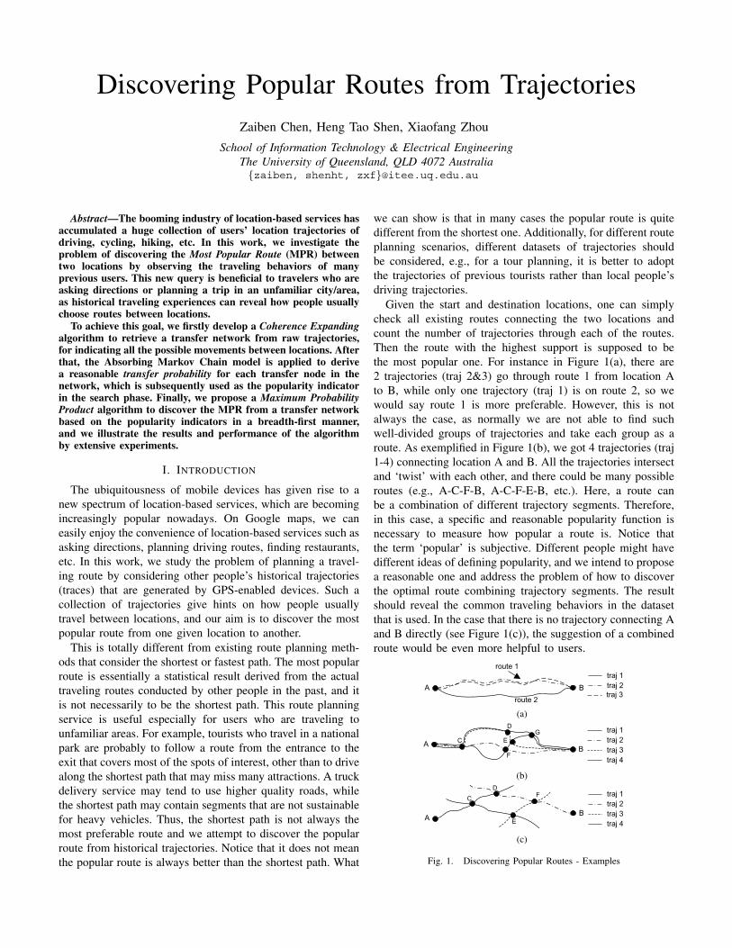
Discovering Popular Routes from TrajectoriesZaiben Chen, Heng Tao Shen, Xiaofang Zhou

School of Information Technology & Electrical EngineeringThe University of Queensland, QLD 4072 Australia{zaiben, shenht, zxf}@itee.uq.edu.au

Abstract—The booming industry of location-based services hasaccumulated a huge collection of users’ location trajectories ofdriving, cycling, hiking, etc. In this work, we investigate theproblem of discovering the Most Popular Route (MPR) betweentwo locations by observing the traveling behaviors of manyprevious users. This new query is beneficial to travelers who areasking directions or planning a trip in an unfamiliar city/area,as historical traveling experiences can reveal how people usuallychoose routes between locations.

To achieve this goal, we firstly develop a Coherence Expandingalgorithm to retrieve a transfer network from raw trajectories,for indicating all the possible movements between locations. Afterthat, the Absorbing Markov Chain model is applied to derivea reasonable transfer probability for each transfer node in thenetwork, which is subsequently used as the popularity indicatorin the search phase. Finally, we propose a Maximum ProbabilityProduct algorithm to discover the MPR from a transfer networkbased on the popularity indicators in a breadth-first manner,and we illustrate the results and performance of the algorithmby extensive experiments.

I. INTRODUCTION

The ubiquitousness of mobile devices has given rise to anew spectrum of location-based services, which are becomingincreasingly popular nowadays. On Google maps, we caneasily enjoy the convenience of location-based services such asasking directions, planning driving routes, finding restaurants,etc. In this work, we study the problem of planning a travel-ing route by considering other people’s historical trajectories(traces) that are generated by GPS-enabled devices. Such acollection of trajectories give hints on how people usuallytravel between locations, and our aim is to discover the mostpopular route from one given location to another.

This is totally different from existing route planning meth-ods that consider the shortest or fastest path. The most popularroute is essentially a statistical result derived from the actualtraveling routes conducted by other people in the past, and itis not necessarily to be the shortest path. This route planningservice is useful especially for users who are traveling tounfamiliar areas. For example, tourists who travel in a nationalpark are probably to follow a route from the entrance to theexit that covers most of the spots of interest, other than to drivealong the shortest path that may miss many attractions. A truckdelivery service may tend to use higher quality roads, whilethe shortest path may contain segments that are not sustainablefor heavy vehicles. Thus, the shortest path is not always themost preferable route and we attempt to discover the popularroute from historical trajectories. Notice that it does not meanthe popular route is always better than the shortest path. What

we can show is that in many cases the popular route is quitedifferent from the shortest one. Additionally, for different routeplanning scenarios, different datasets of trajectories shouldbe considered, e.g., for a tour planning, it is better to adoptthe trajectories of previous tourists rather than local people’sdriving trajectories.

Given the start and destination locations, one can simplycheck all existing routes connecting the two locations andcount the number of trajectories through each of the routes.Then the route with the highest support is supposed to bethe most popular one. For instance in Figure 1(a), there are2 trajectories (traj 2&3) go through route 1 from location Ato B, while only one trajectory (traj 1) is on route 2, so wewould say route 1 is more preferable. However, this is notalways the case, as normally we are not able to find suchwell-divided groups of trajectories and take each group as aroute. As exemplified in Figure 1(b), we got 4 trajectories (traj1-4) connecting location A and B. All the trajectories intersectand ‘twist’ with each other, and there could be many possibleroutes (e.g., A-C-F-B, A-C-F-E-B, etc.). Here, a route canbe a combination of different trajectory segments. Therefore,in this case, a specific and reasonable popularity function isnecessary to measure how popular a route is. Notice thatthe term ‘popular’ is subjective. Different people might havedifferent ideas of defining popularity, and we intend to proposea reasonable one and address the problem of how to discoverthe optimal route combining trajectory segments. The resultshould reveal the common traveling behaviors in the datasetthat is used. In the case that there is no trajectory connecting Aand B directly (see Figure 1(c)), the suggestion of a combinedroute would be even more helpful to users.

BA

traj 1traj 2traj 3

route 1

route 2

(a)

AB

C

D

E

F

G traj 1traj 2traj 3traj 4

(b)

BA

C

D

E

F traj 1traj 2traj 3traj 4

(c)

Fig. 1. Discovering Popular Routes - Examples

Route planning/prediction by driving patterns [1], [2], [3],[4] is more or less similar to our work in analyzing users’traveling behaviors, but they mainly focus on mining thesequential patterns of objects’ trajectories. The sequential pat-terns may help in suggesting a drive turn at some intersectionin a general case, but they are not sufficient and accurateto discover a popular route to some specified destination.For example, we postulate that A-C-D in Figure 1(c) is asequence of locations with high support (i.e. many trajectoriesgo through A-C-D), thus we say A-C-D is a driving pattern.However, people who drive following A-C-D might go to anylocation else rather than our destination B. It is possible thatpeople usually go to B through A-C-E-F, even though thesupport of A-C-E-F is not that high. Therefore, the patternA-C-D is not accurate to reflect users’ behaviors with respectto the destination B, and we have to define new indicatorsto summarize the users’ behaviors with the presence of aspecified destination.

As mentioned above, simply counting the number of tra-jectories is not enough to discover the popular route betweentwo locations, due to the large number of possible routes andthe difficulty in combining trajectory segments. Our basic ideais to construct a transfer network from raw trajectories as anintermediate result to capture the moving behaviors betweenlocations and to facilitate the search of the popular route.Each node in a transfer network is considered as a ‘significantlocation’. We derive the probability of transferring from every‘significant location’ to the destination based on the historicaltrajectories, and the transfer probability is used as an indicatorof popularity. Subsequently, the popularity of a route to thedestination is defined as the product of transfer probabilitiesof all ‘significant locations’ on the route. Thus we focus onusing trajectories to create a general view of traffic which canbe used in a wide range of applications, rather than focusingon common traffic which are of quite limited application only.

To achieve the goal, we propose to tackle a few problems asstated below. (1) Firstly, we need to retrieve a transfer networkfrom a trajectory database to summarize users’ movements.For example in Figure 1(b), the transfer network is comprisedof a set of nodes A to G, which are intersections where peoplebranch off, or the end points of trajectories. We define thesenodes as transfer nodes which are the ‘significant locations’.For any two nodes, if there is any contiguous trajectoryconnecting them without any other nodes in-between, thenthere is a transfer edge between them. So we need to discoverall the transfer nodes and transfer edges as a pre-processingprocedure. Here a Coherence Expanding algorithm that con-siders directional information is developed for mining thetransfer network. (2) The indicators of popularity for transfernodes and routes need to be established. Here we can nolonger use the count number of trajectories as a measurement.The information of the given destination should be consideredas well. We use the Absorbing Markov Chain [5] methodto deduce the transfer probability for each transfer node.By doing so, we provide a reasonable way to measure thepopularity of a route towards the destination, and importantly

the transfer probability of each transfer node supplies a criteriafor the search of the most popular route. (3) Finally, combiningtransfer edges to form the optimal route with respect to thepopularity function is the target we expect to achieve. Basedon the transfer network as well as the transfer probabilities,we propose a Maximum Probability Product algorithm for thesearch of popular routes and briefly prove the accuracy. Thealgorithm shares the same spirit with the Dijkstra’s algorithm[6], and the result route is a path consists of a series of transfernodes that maximizes the product of transfer probabilities.

As a summary, the essence of the route planning approachin this paper is to ‘learn’ from history, and suggest a routeby mining the most popular path from a trajectory databasewhich is modeled as a transfer network. We mainly make thefollowing contributions:

∙ We present a new route planning approach that givesanother option for users other than existing shortest pathbased methods.

∙ We develop an algorithm to establish the transfer networkmodel of a collection of historical trajectories, and utilizethe Absorbing Markov Chain model to derive the transferprobability for transfer nodes.

∙ We propose a reasonable popularity function as well asthe search algorithm for discovering the most popularroute over a transfer network.

∙ We demonstrate the results by extensive experiments.The remainder of the paper is organized as follows. In

section II, the related work is discussed. The mining algorithmfor establishing a transfer network is introduced in section III,and we derive the transfer probabilities in section IV. Thesearch algorithm for discovering the most popular route isstudied in V. Finally we examine the approach in VI and drawa conclusion in section VII. A partial list of the notations usedin this paper are summarized in Table I.

II. RELATED WORK

The search of popular routes in light of past movementsis highly relevant to trajectory processing/querying issues,including pattern mining [7], [2], [1], [8], trajectory clustering[9], [10], hot route discovery [11], [12], trajectory prediction[3], [4], [13], etc. However, none of them addresses theproblem of discovering the most popular route/path from onegiven location to another. Our work is mainly regarding routeplanning issues, while the vast majority of existing work isdealing with a general mining/prediction problem.

The discovery of hot routes in [11] and [12] are themost similar ones to our work in identifying routes that arefrequently visited by users. In [12], Li et al. propose a density-based algorithm FlowScan to extract hot routes according tothe definition of ‘traffic density-reachable’. It is essentially atrajectory clustering algorithm based on traffic density, whichshares the same idea with [9] and [10] that cluster trajectoriesby line segment density. An on-line algorithm is also devel-oped by Sacharidis et al. in [11] for searching and maintaininghot motion paths that are traveled by at least a certain numberof moving objects. Yet, these two work are tailored for mining

paths that are frequently visited from the whole map, whileour work is designed to search the frequently visited path fora query with a start location and a destination.

Mining trajectory patterns [7], [2], [1], [8] could potentiallyhelp in finding a popular route. Giannotti et al. study in [2]the problem of mining T-pattern, which is a sequence oftemporally annotated points, and the target to find out all T-patterns whose support is not less than a support threshold.A T-pattern can naturally be seen as a driving pattern thatindicates a popular movement through a sequence of points.Hence, if the given start and end locations are just right onthe sequence, we may suggest the sequence to the user as arecommended route. However, not every pair of start and endlocations are able to match with an existing pattern, so thisapproach does not work for the planning of a route betweentwo arbitrary locations. Besides, region of interest (ROI) isused for approximating a trajectory as a sequence of symbols,which is not accurate enough in showing detailed directionsfor route planning purpose. Similarly in [1] and [8], existingsequential pattern mining algorithms are adopted to explorefrequent path segments or sequences of points. In [7], miningperiodic movements through regions is investigated as well.

In the pre-processing phase of our solution, a coherenceexpanding algorithm is developed for retrieving all road in-tersections from raw trajectories, and subsequently the wholetransfer network. The rationale of this algorithm is similarto the density-based clustering algorithm DBSCAN in [14],which expands a cluster from a seed point. However, weuse a different connectivity function and different settings forcapturing the specific features of road intersections, comparedwith merely the density of points used in DBSCAN. In [15],Cao et al. also propose an approach to retrieve a road networkfrom trajectories. However, their method is mainly designedfor identifying edges while road intersections are not elegantlyclarified. The work in [16] is particularly designed for discov-ering road intersections, but they require an underlying roadmap available in advance for training a classifier, while in ouralgorithm, the trajectories may be un-constraint and the roadmap availability is not assumed.

Other related work includes path planning by consideringtraffic uncertainty [17], searching similar trajectories [18],[19], [20], [21], [22], shortest path [6], [23], shortest pathon time-dependent networks [24], finding the fastest path byspeed patterns [25], etc. Nevertheless, all the work above isnot able to address the problem of capturing and deriving thepopularity of a route between two given locations.

III. MINING TRANSFER NETWORK

In order to systematically analyze the users’ traveling behav-iors through GPS trajectories, first of all we establish a transfernetwork from raw trajectories. The transfer network is ineffect a directional graph 𝐺(𝑁,𝐸) indicating the movementsbetween locations. Here 𝑁 is a set of transfer nodes, whichcan be an intersection of trajectories or just the end locationsof a trajectory. An intersection is physically a small region thattrajectories from/to different directions come across, and these

TABLE IA LIST OF NOTATIONS

Notation Explanation𝑐𝑜ℎ(𝑝, 𝑞) The coherence between point 𝑝 and 𝑞𝛿 The scaling factor𝜃 The angle of difference between two mov-

ing directions𝛼, 𝛽 The tuning parameters𝜏, 𝜑 The coherence and the group size thresholds𝑝⊖ 𝑞 𝑝 is directly coherence-connected with 𝑞𝑝⊘ 𝑞 𝑝 is coherence-connected with 𝑞𝑃𝑟(𝑛𝑖 → 𝑛𝑗) The turning probability of moving from 𝑛𝑖

to 𝑛𝑗

𝑃𝑟𝑑(𝑛𝑖 → 𝑛𝑗) The turning probability of moving from 𝑛𝑖

to 𝑛𝑗 w.r.t. a destination 𝑑𝑝𝑡𝑛𝑖,𝑛𝑗

The probability of first arrival at 𝑛𝑗 , startingfrom 𝑛𝑖, in exactly 𝑡 steps

𝑃𝑟𝑡(𝑛𝑖 → 𝑑) The transfer probability of going from 𝑛𝑖

to 𝑑 within 𝑡 steps𝑉 The column vector of transfer probabilities

for all nodes𝑅 A route𝜌(𝑅) The popularity of route 𝑅

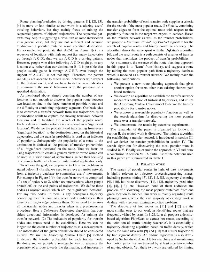
locations are supposed to be ‘significant’ in our model sincethey are the positions where people can make a turn. 𝐸 is acollection of transfer edges connecting transfer nodes. We saythere exists an edge 𝑒 from node 𝐴 to 𝐵 if there is at least onecontiguous trajectory from 𝐴 to 𝐵 without any other transfernodes in-between. Besides, for trajectories that move in thesame direction between two adjacent nodes, we group theminto the same edge. Consequently, we transform trajectoriesinto a routable directional network. As illustrated in Figure 2,we aim to acquire the network (refer to Figure 2(b)) from aset of raw trajectories as plotted in Figure 2(a). In Figure 2(b),a dot represents a transfer node and a line indicates a transferedge. Notice that if there is a road map available, we can findout the transfer network by map-matching [26] trajectories,but here we attempt to make this work compatible with bothconstraint and un-constraint trajectories. Typically, traces ofhiking, boating, walking, and many out-door activities are notconstrained by a road network, and most maps that peoplethink of as free actually have legal or technical restrictions ontheir use [27], [28], which hold back people from using themin creating new applications.

(a) Distribution of Trajectory Points (b) Transfer Network

Fig. 2. Mining Transfer Network (trajectory end points not shown)

The problem arising here is how to detect the intersectionsof trajectories if there is no map available. Firstly, let’s repre-sent a GPS trajectory by a series of points {𝑝1, 𝑝2, ⋅ ⋅ ⋅ , 𝑝𝑛},where 𝑝𝑖 indicates a recorded position (𝑙𝑜𝑛𝑔𝑖𝑡𝑢𝑑𝑒, 𝑙𝑎𝑡𝑖𝑡𝑢𝑑𝑒),and the moving direction of 𝑝𝑖 is −−−−→𝑝𝑖𝑝𝑖+1. We have thefollowing observations upon trajectory intersections:

1) Within an intersection region, the density of trajectorypoints is normally higher, in comparison with the densityof points on an incoming/outgoing road edge, becauseit is the place where trajectories join together or driversslow down to make a turn. If we consider an intersectionas a group of points, then the size of the group shouldbe greater than some threshold.

2) A number of trajectories change moving direction at anintersection, as some people make turns. The movingdirections of trajectory points from/to different roadedges are likely to be orthogonal (i.e., angle of differencetends to 𝜋/2). Within a small distance, points whosemoving directions differ by 0 or 𝜋 (i.e., in the sameor opposite direction) are probably on the same road,while points with direction difference > 0 and < 𝜋are possibly moving to different road branches of anintersection. The closer the angle of difference tends to𝜋/2, the higher possibility that an intersection exists.

Thus the intuition is that we can find intersections bymining groups (clusters) of points that satisfy both densityand direction conditions. However, for point density, it candiffer greatly at different intersections since there may betens of thousands of points recorded at a hot intersectionwhile only a few points at an un-popular one. Therefore, wemerely set group size threshold as a post-filtering parameterand the mining algorithm mainly distinguishes intersectionsby the moving direction information. Before describing ouralgorithm, we firstly list some definitions.

Definition 1: Coherence. Given two trajectory points 𝑝 and𝑞, the coherence 𝑐𝑜ℎ between them is defined as:

𝑐𝑜ℎ(𝑝, 𝑞) = exp(−(𝑑𝑖𝑠𝑡(𝑝, 𝑞)

𝛿

)𝛼

) ⋅ ∣ sin 𝜃∣𝛽 (1)

Here 𝑑𝑖𝑠𝑡(𝑝, 𝑞) is the Euclidean distance between 𝑝 and𝑞. 𝛿 is a scaling factor. 𝜃 is the angle of difference between𝑝 and 𝑞’s moving directions, which ranges from 0 to 𝜋. 𝛼and 𝛽 are tuning parameters, and we will discuss setting𝛼, 𝛽 in the experiment section. In Equation 1, the partexp(−(𝑑𝑖𝑠𝑡(𝑝,𝑞)𝛿 )𝛼) scores the coherence by distance, and itdecreases exponentially as 𝑑𝑖𝑠𝑡(𝑝, 𝑞) goes up. sin 𝜃, on theother hand, specifies that only points with 𝜃 → 𝜋/2 canretain a strong coherence. Obviously, points on an transferedge have a low coherence as they move in a similar direction(sin 𝜃 → 0), and only points that are close to each other at anintersection and towards different directions will have a strongcoherence.

Definition 2: Directly Coherence-Connected. Given a co-herence threshold 𝜏 , a point 𝑝 is directly coherence-connectedwith another point 𝑞 w.r.t. 𝜏 if and only if 𝑐𝑜ℎ(𝑝, 𝑞) ≥ 𝜏 , andwe denote this relation by 𝑝⊖ 𝑞.

It is straightforward that the relation of Directly Coherence-Connected is symmetric for any pair of points, since𝑐𝑜ℎ(𝑝, 𝑞) = 𝑐𝑜ℎ(𝑞, 𝑝). However, it is not transitive, whichmeans (𝑝⊖ 𝑞 ∧ 𝑞 ⊖ 𝑟) does not imply 𝑝⊖ 𝑟.

Definition 3: Coherence-Connected. A point 𝑝 iscoherence-connected with a point 𝑞 w.r.t. 𝜏 if there is a chainof points 𝑝1, 𝑝2, ⋅ ⋅ ⋅ , 𝑝𝑛, 𝑝1 = 𝑝, 𝑝𝑛 = 𝑞, such that 𝑝𝑖 ⊖ 𝑝𝑖+1.We denote this relation by 𝑝⊘ 𝑞.

12

2

1

Fig. 3. Coherence-Connected

Considering the example in Figure 3, the coherence between𝑝1 and 𝑝2 on 𝑡𝑟𝑎𝑗 1 is very low as the 𝜃 between their movingdirections is about 0, thus they are not directly coherence-connected. However, 𝑞2 on 𝑡𝑟𝑎𝑗 2 (in a very different direc-tion) is directly coherence-connected with both 𝑝1 and 𝑝2,(i.e., 𝑝1⊖ 𝑞2 & 𝑞2⊖ 𝑝2), thus 𝑝1⊘ 𝑝2. Obviously, Coherence-Connected is a symmetric and transitive relation. We have𝑝 ⊘ 𝑞 → 𝑞 ⊘ 𝑝, and 𝑝 ⊘ 𝑞 ∧ 𝑞 ⊘ 𝑟 → 𝑝 ⊘ 𝑟. Importantly, byusing the coherence-connected relation, we are able to definea cluster as a set of coherence-connected trajectory points.The rationale is similar to that of the DBSCAN clustering[14]. Such a cluster contains a group of points sticked togetherby coherence, which typically appears only at an intersection(road cross or turning corner) where direction changes canhappen. Note that GPS errors may also cause direction changesand that is why we clean the dataset first before clustering.

Definition 4: Cluster. Assume 𝑂 is the complete set oftrajectory points. Given the coherence threshold 𝜏 and thecluster size threshold 𝜑, a cluster 𝐶 w.r.t. 𝜏 and 𝜑 is a subsetof 𝑂 satisfying the following conditions:

1) If a point 𝑝 ∈ 𝐶 and 𝑝 is coherence-connected with 𝑞w.r.t. 𝜏 , then 𝑞 ∈ 𝐶. (Maximality)

2) For any pair of 𝑝, 𝑞 ∈ 𝐶 (𝑝 ∕= 𝑞), 𝑝 and 𝑞 are coherence-connected w.r.t. 𝜏 . (Connectivity)

3) The size of 𝐶 ≥ 𝜑.This definition looks similar to the density-connected cluster

[14], but here we apply a different connectivity function forclustering intersections other than finding groups of densepoints. Any two points 𝑝, 𝑞 in a cluster 𝐶 are coherence-connected, which means there are always a series of points𝑝1, 𝑝2, ⋅ ⋅ ⋅ , 𝑝𝑛, (𝑝1 = 𝑝, 𝑝𝑛 = 𝑞), such that 𝑝𝑖 and 𝑝𝑖+1

are directly coherence-connected. Therefore, we are able toexplore from any 𝑝 to any 𝑞 through the Directly Coherence-Connected relation. Intuitively, given a point 𝑝 in 𝐶 as a seedof the cluster, we can discover the cluster by expanding from𝑝 outwards through exploring surrounding points that are di-rectly coherent-connected with the seed. The new found pointsare then used as seeds for finding more directly coherent-connected points. This is also the basic idea of our CoherenceExpanding algorithm.

Lemma 1: Let 𝑝, 𝑞 ∈ 𝑂 be any two points that arecoherence-connected, 𝐶1 = {𝑜∣𝑜 ∈ 𝑂 ∧ 𝑜 ⊘ 𝑝}, and 𝐶2 ={𝑜∣𝑜 ∈ 𝑂 ∧ 𝑜⊘ 𝑞}, then we have 𝐶1 = 𝐶2.

Proof: For any point 𝑜 ∈ 𝐶1, we have 𝑜⊘𝑝. Since ⊘ is atransitive relation and 𝑝⊘𝑞, it is clear that for any 𝑜 ∈ 𝐶1, wealso have 𝑜⊘𝑞. Consequently, all points in 𝐶1 are included in𝐶2 according to the definition of 𝐶2, (i.e. 𝐶1 ⊆ 𝐶2). Similarlywe can prove that 𝐶2 ⊆ 𝐶1. Therefore, we have 𝐶1 = 𝐶2.

Lemma 1 tells that the expanding results of any twocoherence-connected points are exactly the same. For findinga cluster, we can arbitrarily choose any point of the cluster asa seed and expand for the whole set of points of the cluster.This also means that a cluster is uniquely determined by anyof it’s points.

Lemma 2: Let 𝑝 ∈ 𝑂 be any point of a cluster 𝐶. We have𝐶 = {𝑜∣𝑜 ∈ 𝑂 ∧ 𝑜⊘ 𝑝}.

Lemma 2 is a straightforward conclusion according toLemma 1 and Definition 4. Based on Lemma 2, we develop theCoherence Expanding algorithm for clustering intersections.

Algorithm 1: Coherence Expandinginput : A set of trajectory points 𝑃 ; Threshold 𝜏, 𝜑;output: clusters[]for each point 𝑝 ∈ 𝑃 do1

if p.classified=false then2

𝑝.classified ← true;3

cluster = expand(𝑝);4

if cluster.size ≥ 𝜑 then5

clusters.add(cluster);6

return clusters;7

In Algorithm 1, we simply check each trajectory point in 𝑃sequentially. If it has not been classified to any cluster yet, wetry to expand it by using the Directly Coherence-Connectedrelation at line 4. After that if the size of the returned setof points exceeds or is equal to the threshold 𝜑, then the setis stored as a valid cluster. By doing so, eventually all validclusters will be found, since once we start checking any pointof a cluster, all the other points of the cluster will be retrievedin the expanding procedure. For those points not belonging toany valid cluster, we just skip them.

Algorithm 2: expand(𝑝)input : A point 𝑝output: A set of points 𝑟𝑒𝑠𝑢𝑙𝑡Queue seeds ← new Queue();1

seeds.add(𝑝);2

𝑟𝑒𝑠𝑢𝑙𝑡.add(𝑝);3

while seeds ∕= 𝑛𝑢𝑙𝑙 do4

𝑠𝑒𝑒𝑑 ← seeds.pop();5

points ← rangeQuery(𝑠𝑒𝑒𝑑, 𝑟𝑎𝑑𝑖𝑢𝑠);6

for i=0 ; i < points.size ; i++ do7

𝑝𝑡 ← points.get(𝑖);8

if 𝑝𝑡.classified=false ∧ 𝑐𝑜ℎ(𝑠𝑒𝑒𝑑, 𝑝𝑡) ≥ 𝜏 then9

seeds.add(𝑝𝑡);10

𝑟𝑒𝑠𝑢𝑙𝑡.add(𝑝𝑡);11

return 𝑟𝑒𝑠𝑢𝑙𝑡;12

In the expanding procedure as shown in Algorithm 2, wemaintain a queue of seeds, which contains only the given point𝑝 initially (line 1-2). Then we go to the 𝑤ℎ𝑖𝑙𝑒 loop to checkeach of the seeds and search for more surrounding points asseeds by a range query centered at 𝑠𝑒𝑒𝑑 with a given 𝑟𝑎𝑑𝑖𝑢𝑠at line 6. Here, the range query is conducted over an R-tree[29] index of all trajectory points. After that, we examine eachof the points that fall in range. If a point 𝑝𝑡 is not classifiedyet and is directly coherence-connected with the 𝑠𝑒𝑒𝑑 fromwhich 𝑝𝑡 is discovered by the range query (line 9), we add itto the queue as a new seed and append it to the result set (line10-11). In such a way, we expand the result set from 𝑝 until nomore directly coherence-connected points can be found, andreturn the set as a final complete cluster (intersection).

Regarding the 𝑟𝑎𝑑𝑖𝑢𝑠 of the range query at line 6 inAlgorithm 2, if it is too small, we may miss some directlycoherence-connected points. If it is too large, extra effort isneeded to examine un-qualified points. Hence we set the radiusas the largest distance 𝑑𝑖𝑠𝑡 satisfying 𝑐𝑜ℎ𝑒𝑟𝑒𝑛𝑐𝑒 ≥ 𝜏 . That is:

exp(−(𝑑𝑖𝑠𝑡𝛿

)𝛼) ⋅ (sin 𝜃)𝛽 ≥ 𝜏

Let 𝜃 = 𝜋/2. By solving the inequation above, the maximalvalue of 𝑑𝑖𝑠𝑡 is found out to be:

𝑑𝑖𝑠𝑡 = 𝛿 ⋅ 𝛼√− ln(𝜏)

For points with a larger distance than 𝑑𝑖𝑠𝑡 from a 𝑠𝑒𝑒𝑑, theymust have a coherence less than 𝜏 , and thus 𝑑𝑖𝑠𝑡 is a safedistance to include all possible cluster points.

In practice, as GPS data is more or less dirty, we firstreduce outlier points that suddenly jump away by consideringphysical limits on vehicle speed, before running the clusteringalgorithm. Besides, linear interpolation is conducted for lowsampling-rate trajectories to reduce the possibility that theyare missed at some intersections that they do pass through.Direction smoothing is also carried out to alleviate the effect ofposition fluctuation caused by GPS inaccuracy. This cleaningprocedure is mainly based on common sense, and it is just forproviding a higher quality dataset.

After discovering all the clusters (intersections), we treateach of them as a transfer node whose location is approximatedby the average coordinate, while transfer edges are constructedby checking trajectories between nodes. As exemplified inFigure 2, we group 292,394 trajectory points into a transfernetwork with 424 nodes (end points of trajectories are notshown here). The benefits of clustering are two-fold. Firstlyit summarizes movements by a network which is easier toanalyze, and secondly it significantly reduces the numberof nodes that need to be considered in the analyzing step.The complexity of the Coherence Expanding algorithm isobviously: number of points × cost of a range query.

IV. DERIVING TRANSFER PROBABILITY

Through the Coherence Expanding algorithm, we can re-trieve a directional transfer network 𝐺(𝑁,𝐸) from raw trajec-tories. In this section, we analyze the users’ traveling behaviors

on a network, and deduce the transfer probabilities of nodesw.r.t. a given destination. The aim is to find out which transfernode is more likely to lead a user to the destination, and thisprobability will serve as a popularity indicator.

At a transfer node 𝑛𝑖, a simple way of observing users’historical behaviors is to enumerate all adjacent edges thatstart from 𝑛𝑖 and check how many people ever passed eachof them. The turning probability of moving from 𝑛𝑖 to anoutgoing edge 𝑒 = (𝑛𝑖, 𝑛𝑗) will then be:

𝑃𝑟(𝑛𝑖 → 𝑛𝑗) =number of trajectories on (𝑛𝑖, 𝑛𝑗)

number of trajectories on all outgoing edges

However, this statistics of user behaviors is just for a generalcircumstance without the consideration of destination. That is,this statistics is purely about how people generally make turnsat 𝑛𝑖, and people might just go to any destination. Therefore,when asking about the turning probability at a node w.r.t. agiven destination, we should further consider if the historicaltrajectories that the node contains are (approximately) headingthe destination or not to define a more reasonable probabilityfunction. We modify the previous equation and define theturning probability w.r.t. a destination 𝑑 as follows:

𝑃𝑟𝑑(𝑛𝑖 → 𝑛𝑗) =

∑𝑡𝑟𝑎𝑗∈(𝑛𝑖,𝑛𝑗)

𝑓𝑢𝑛𝑐(𝑡𝑟𝑎𝑗, 𝑑)∑𝑡𝑟𝑎𝑗∈all outgoing edges 𝑓𝑢𝑛𝑐(𝑡𝑟𝑎𝑗, 𝑑)

(2)

The only difference here is that we use a function𝑓𝑢𝑛𝑐(𝑡𝑟𝑎𝑗, 𝑑) to score how likely a trajectory 𝑡𝑟𝑎𝑗 mightsuggest a correct route to 𝑑. We have confidence that atrajectory approximately heading the destination will probablygive a correct hint on how to take the next edge to go. Weestimate this likelihood by:

𝑓𝑢𝑛𝑐(𝑡𝑟𝑎𝑗, 𝑑) = exp (−𝑑𝑖𝑠𝑡𝑠(𝑡𝑟𝑎𝑗, 𝑑))where 𝑑𝑖𝑠𝑡𝑠(𝑡𝑟𝑎𝑗, 𝑑) is the shortest Euclidean/network dis-tance between 𝑑 and the front part of 𝑡𝑟𝑎𝑗 that starts from𝑛𝑖. Apparently, if the front part of 𝑡𝑟𝑎𝑗 passes through 𝑑exactly, the distance is 0 and thus the likelihood is 1. The largerdistance 𝑡𝑟𝑎𝑗 deviates from 𝑑, the lower likelihood it willbe assigned. Consequently, outgoing edges with trajectoriesclose to the destination are associated with higher turningprobability, compared with those edges that keep away from𝑑. Therefore, in Equation 2, we provide a simple way to definethe probability indicating how users made turns at a transfernode for the purpose of going to a given destination, byconsidering both the number of trajectories and their distancesto the destination, which addresses the problems discussed inFigure 1(a) and 1(c) in the introduction section.

Furthermore, we can consider a travel on such a transfernetwork based on the turning probability as a Random Walk[30] on a directed graph with the transition probability fromnode 𝑛𝑖 to 𝑛𝑗 equals to 𝑃𝑟𝑑(𝑛𝑖 → 𝑛𝑗). If we conduct sucha random walk on a transfer network following the turningprobability, we will probably reach the destination as wealways tend to select an edge that is most likely to lead tothe destination. However, one question is that:

If we conduct such a random walk, what is the exactprobability that, starting from a node 𝑛𝑖, we will eventuallyreach the destination 𝑑 within 𝑡 steps?

We call this probability the transfer probability which takes𝑡 following transfers into account. In this way, we furtherconsider all possible connecting edges within 𝑡 steps afterleaving 𝑛𝑖, which solves the problem raised in Figure 1(b).Apparently, the larger transfer probability a node 𝑛𝑖 holds,the higher confidence we have that 𝑛𝑖 will lead us to thedestination. Denote by 𝑁𝑡 the node that we arrive at after𝑡 transfers, and by 𝑝𝑡𝑛𝑖,𝑛𝑗

the probability that, starting at node𝑛𝑖, we first arrive at node 𝑛𝑗 in exactly 𝑡 steps. We have:

𝑝𝑡𝑛𝑖,𝑛𝑗= 𝑃𝑟(𝑁𝑡 = 𝑛𝑗 and, for 1 ≤ 𝑙 < 𝑡,𝑁𝑙 ∕= 𝑛𝑗 ∣𝑁0 = 𝑛𝑖)

(3)In Equation 3, 𝑝𝑡𝑛𝑖,𝑛𝑗

is defined as the probabilitythat, starting from 𝑁0 = 𝑛𝑖, all the intermediate nodes𝑁1, 𝑁2, ⋅ ⋅ ⋅ , 𝑁𝑡−1 are not 𝑛𝑗 , and we arrive at 𝑛𝑗 at exactlythe 𝑡𝑡ℎ step. The transfer probability 𝑃𝑟𝑡(𝑛𝑖 → 𝑑) of goingfrom any 𝑛𝑖 to destination 𝑑 within 𝑡 steps is in fact the sumof probability that we first arrive at 𝑑 in 1, 2, ⋅ ⋅ ⋅ , 𝑡 step.Consequently, we have:

𝑃𝑟𝑡(𝑛𝑖 → 𝑑) =

𝑡∑𝑗=1

𝑝𝑗𝑛𝑖,𝑑(4)

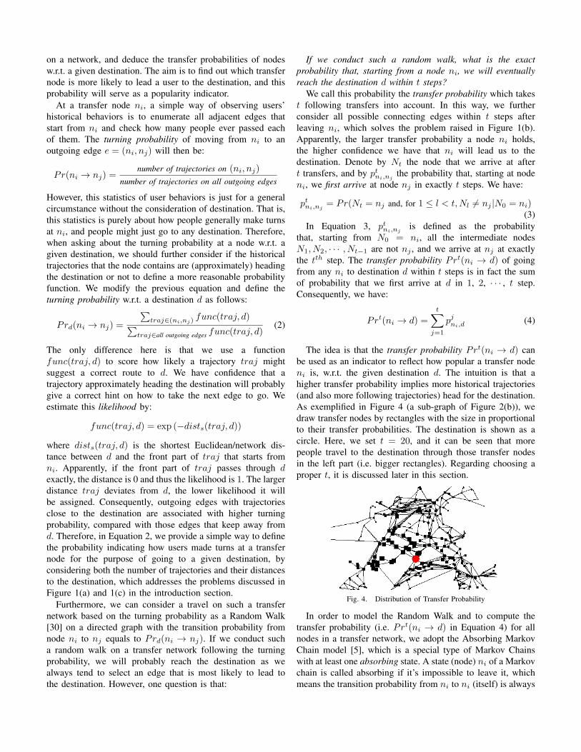
The idea is that the transfer probability 𝑃𝑟𝑡(𝑛𝑖 → 𝑑) canbe used as an indicator to reflect how popular a transfer node𝑛𝑖 is, w.r.t. the given destination 𝑑. The intuition is that ahigher transfer probability implies more historical trajectories(and also more following trajectories) head for the destination.As exemplified in Figure 4 (a sub-graph of Figure 2(b)), wedraw transfer nodes by rectangles with the size in proportionalto their transfer probabilities. The destination is shown as acircle. Here, we set 𝑡 = 20, and it can be seen that morepeople travel to the destination through those transfer nodesin the left part (i.e. bigger rectangles). Regarding choosing aproper 𝑡, it is discussed later in this section.

Fig. 4. Distribution of Transfer Probability

In order to model the Random Walk and to compute thetransfer probability (i.e. 𝑃𝑟𝑡(𝑛𝑖 → 𝑑) in Equation 4) for allnodes in a transfer network, we adopt the Absorbing MarkovChain model [5], which is a special type of Markov Chainswith at least one absorbing state. A state (node) 𝑛𝑖 of a Markovchain is called absorbing if it’s impossible to leave it, whichmeans the transition probability from 𝑛𝑖 to 𝑛𝑖 (itself) is always

1, while those non-absorbing states are called transient states.In our directional transfer network, the destination node 𝑑 istreated as an absorbing state, since whenever we arrive, we juststay there and we don’t consider a route to 𝑑 that passes thedestination more than once. Additionally, those end points oftrajectories without any outgoing edges are also considered asabsorbing states since one can not move from them to anothernode in a directional network. All other transfer nodes areconsidered as transient states. The transition matrix 𝑃 for 𝑚transfer nodes can be represented by:

𝑃 =

𝑛1 𝑛2 ⋅ ⋅ ⋅ 𝑛𝑚

𝑛1 𝑃 (1, 1) 𝑃 (1, 2) ⋅ ⋅ ⋅ 𝑃 (1,𝑚)𝑛2 𝑃 (2, 1) 𝑃 (2, 2) ⋅ ⋅ ⋅ 𝑃 (2,𝑚)...

......

. . ....

𝑛𝑚 𝑃 (𝑚, 1) 𝑃 (𝑚, 2) ⋅ ⋅ ⋅ 𝑃 (𝑚,𝑚)

where the entry 𝑃 (𝑖, 𝑗) denotes the transition probability ofmoving from node 𝑛𝑖 to 𝑛𝑗 as defined in Equation 5.

𝑃 (𝑖, 𝑗) =

{1 if 𝑛𝑖 is an absorbing state & 𝑖 = 𝑗𝑃𝑟𝑑(𝑛𝑖 → 𝑛𝑗) if 𝑛𝑖 is a transient state & 𝑖 ∕= 𝑗0 otherwise

(5)For absorbing states, they transfer to themselves with prob-ability 1, while transient states make transitions to adjacentnodes according to the turning probability determined byEquation 2. The purpose of adopting the Absorbing MarkovChain model to represent a transfer network is for figuringout the probability of the first arrival to 𝑑 (i.e., 𝑝𝑡𝑛𝑖,𝑑

), andconsequently 𝑃𝑟𝑡(𝑛𝑖 → 𝑑).

Assume there are totally 𝑥 absorbing states, and 𝑦 transientstates (𝑥+ 𝑦 = 𝑚). We group absorbing states into ABS andtransient states into TR, then the transition matrix 𝑃 can bere-organized in the following canonical form [5]:

𝑃 =TR ABS

TR Q SABS 0 I

(6)

I is a 𝑥− 𝑏𝑦−𝑥 identity matrix, 0 is a 𝑥− 𝑏𝑦−𝑦 zero matrix,𝑄 is a 𝑦 − 𝑏𝑦 − 𝑦 matrix indicating the transition probabilitybetween transient states, and 𝑆 is a 𝑦−𝑏𝑦−𝑥 matrix indicatingthe transition probability from transient states to absorbingstates. To acquire the transition probability from node 𝑛𝑖 to𝑛𝑗 in exactly 𝑡 steps, we take the 𝑡𝑡ℎ power of 𝑃 and we get:

𝑃 𝑡 =TR ABS

TR Q𝑡 ∗ABS 0 I

(7)

where 𝑄𝑡 is the 𝑡𝑡ℎ power of 𝑄, and ∗ is a 𝑦− 𝑏𝑦− 𝑥 matrixwritten in terms of 𝑄 and 𝑆. From the Markov Chain theory,we know that the (𝑖, 𝑗)𝑡ℎ entry 𝑃 𝑡(𝑖, 𝑗) of the matrix 𝑃 𝑡 is theprobability of being at the state 𝑛𝑗 after 𝑡 steps, starting from𝑛𝑖. Nevertheless, 𝑃 𝑡(𝑖, 𝑗) is not equal to the 𝑝𝑡𝑛𝑖,𝑛𝑗

definedin Equation 3, as 𝑝𝑡𝑛𝑖,𝑛𝑗

has to be the probability of thefirst arrival while 𝑃 𝑡(𝑖, 𝑗) does not guarantee this condition.However, we don’t need to know 𝑝𝑡𝑛𝑖,𝑛𝑗

for all 𝑛𝑗 , but just

𝑝𝑡𝑛𝑖,𝑑for the destination 𝑑 that is an absorbing state. This

makes the problem simpler, and we have the following lemma.Lemma 3: A route that first visits the destination in exactly

(𝑡 > 0) steps (transfers), must start from a transient state, andthe state at 𝑡 = 1, 2, ⋅ ⋅ ⋅ , 𝑡− 1 step is also a transient state.

Proof: If we start from or visit any absorbing state otherthan the destination before arriving at the destination node,we are not able to get to the destination as an absorbing statealways transfers to itself. Therefore, the lemma is proved.

Since the 1𝑠𝑡 to (𝑡 − 1)𝑡ℎ states of a route are transient, aroute must transfer between transient states for 𝑡−1 times andfinally jump from a transient state to the destination at the 𝑡𝑡ℎ

step. For the first (𝑡− 1)-step transfer, it’s probability can beacquired from 𝑄𝑡−1, while the probability of moving from atransient state to the destination is given in 𝑆. Consequently,the 𝑝𝑡𝑛𝑖,𝑑

for a given 𝑛𝑖 can be computed in the following way:

𝑝𝑡𝑛𝑖,𝑑 =∑

𝑛𝑘∈TR

(𝑃 𝑡−1(𝑖, 𝑘) ⋅ 𝑃 (𝑘, 𝑑)

)(8)

where 𝑃 𝑡−1(𝑖, 𝑘) is the probability of transferring from 𝑛𝑖 toanother transient state 𝑛𝑘 in exactly 𝑡 − 1 steps, and 𝑃 (𝑘, 𝑑)is the probability of transferring from 𝑛𝑘 to the destination 𝑑in one step. Apparently, 𝑃 𝑡−1(𝑖, 𝑘) is an entry of 𝑄𝑡−1 in theupper-left block of the matrix 𝑃 𝑡−1 (refer to the canonicalform in Equation 7), and 𝑃 (𝑘, 𝑑) is an entry of 𝑆 in theupper-right block of the matrix 𝑃 in Equation 6. Therefore,by combining Equation 4 and 8, the transfer probability of agiven node 𝑛𝑖 w.r.t. 𝑑 and 𝑡 is determined by:

𝑃𝑟𝑡(𝑛𝑖 → 𝑑) =∑𝑡

𝑗=1 𝑝𝑗𝑛𝑖,𝑑

=∑𝑡

𝑗=1

∑𝑛𝑘∈TR

(𝑃 𝑗−1(𝑖, 𝑘) ⋅ 𝑃 (𝑘, 𝑑)

)(9)

Note that when 𝑗 = 1, it goes from a transient state 𝑛𝑘 to𝑑 directly in one step and we set 𝑃 0(𝑖, 𝑘) = 1. To computethe transfer probability for each transfer node that belongs totransient states, we may conduct the computation by matrixmultiplications. Assume 𝑛1, 𝑛2, ⋅ ⋅ ⋅ , 𝑛𝑙 are the transient nodesin TR. We suppose to derive the column vector:

𝑉 =[𝑃𝑟𝑡(𝑛1 → 𝑑), 𝑃 𝑟𝑡(𝑛2 → 𝑑), ⋅ ⋅ ⋅ , 𝑃 𝑟𝑡(𝑛𝑙 → 𝑑)

]𝑇for a given destination 𝑑 and parameter 𝑡. Now we have 𝑄 and𝑆 from Equation 6, and 𝑑 is included in ABS. Let’s denoteby 𝐷 the column vector corresponding to node 𝑑 in the sub-matrix 𝑆 (i.e., 𝐷 = 𝑆[∗, 𝑑]). The result 𝑉 is calculated by:

𝑉 = 𝐷 +𝑄 ⋅𝐷 +𝑄2 ⋅𝐷 + ⋅ ⋅ ⋅+𝑄𝑡−1 ⋅𝐷 (10)

An example result of 𝑉 has been shown in Figure 4where we show the transfer probability of transfer nodes byrectangles in different sizes. Since each node can potentiallybe the destination, we pre-compute the vector 𝑉 for eachtransfer node assuming it as the destination, and record all 𝑉for the purpose of searching the most popular route. Totally, itconsumes 𝑂(𝑚2) space for storing the pre-computed vectors,if there are 𝑚 transfer nodes. The computation involves 𝑡− 1matrix multiplications of 𝑄 that causes 𝑂(𝑡×𝑚3) complexity

in CPU time. Algorithm 3 lists the procedures for deriving thetransfer probabilities for a transfer network 𝐺(𝑁,𝐸).

Algorithm 3: Deriving Transfer Probability

input : A transfer network 𝐺(𝑁,𝐸)output: A vector 𝑉 for each node ∈ 𝑁for each transfer node 𝑛𝑖 ∈ 𝑁 do1

set 𝑛𝑖 as the destination;2

construct the transition matrix 𝑃 by Equation 5;3

re-organize 𝑃 in a canonical form;4

acquire 𝑄, 𝑆 from 𝑃 ;5

derive 𝑉 by Equation 10;6

store 𝑉 ;7

Choosing a proper 𝑡 is also important in the derivationof transfer probabilities. It specifies the maximum step wetake into account, and the length of the longest route thatwe consider. For a route whose length is excessively large,it does not make any sense as people would not take such aroute to travel. On the other hand, if 𝑡 is small, for example,even smaller than the step number of the shortest route tothe destination, then we fail to discover a route for the userbecause there is no route that can reach the destination within𝑡 steps (i.e., transfer probability = 0). Considering the twofactors, we set 𝑡 as the diameter of the transfer network inour experiments, which guarantees at least one route can befound between any two nodes and also avoids consideringthose excessively long routes.

If a user starts from a trajectory end point that belongs toabsorbing states, then no route exists in the directional net-work. An alternative solution is to extend the transfer networkto an un-directional one with minor additional changes.

V. SEARCHING THE MOST POPULAR ROUTE

Through mining transfer network and the derivation oftransfer probabilities, we acquire a directional transfer network𝐺(𝑁,𝐸) with a set of transfer probability vectors (𝑉 ) indi-cating how possible a transfer node would lead one to his/herdestination 𝑑. We take the transfer probability of a transfernode 𝑛𝑖 w.r.t. 𝑑 as the popularity indicator:

𝑛𝑖.𝑝𝑜𝑝𝑢𝑙𝑎𝑟𝑖𝑡𝑦(𝑑) = 𝑃𝑟𝑡(𝑛𝑖 → 𝑑)

If 𝑛𝑖 = 𝑑, we assume 𝑛𝑖.𝑝𝑜𝑝𝑢𝑙𝑎𝑟𝑖𝑡𝑦(𝑑) = 1, and if 𝑛𝑖 is atrajectory end point that belongs to absorbing states, we set𝑛𝑖.𝑝𝑜𝑝𝑢𝑙𝑎𝑟𝑖𝑡𝑦(𝑑) = 0. Each transfer node 𝑛𝑖 maintains 𝑚 in-dicators: 𝑛𝑖.𝑝𝑜𝑝𝑢𝑙𝑎𝑟𝑖𝑡𝑦(𝑛1), ⋅ ⋅ ⋅ , 𝑛𝑖.𝑝𝑜𝑝𝑢𝑙𝑎𝑟𝑖𝑡𝑦(𝑛𝑚), for all𝑚 nodes in the transfer network which are potential destina-tions. An indicator conveys the popularity that people take thetransfer node for going to the corresponding destination. In thefollowing we study how to discover the most popular route inlight of the node popularity indicators. Firstly, we have somedefinitions:

Definition 5: Route. A route 𝑅 is defined as a consecu-tive sequence of transfer nodes 𝑛1 → 𝑛2 → ⋅ ⋅ ⋅𝑛𝑖, where(𝑛𝑗 , 𝑛𝑗+1), (1 ≤ 𝑗 < 𝑖), is an existed transfer edge.

Definition 6: Route Popularity. The popularity 𝜌(𝑅) of aroute 𝑅 = 𝑛1 → 𝑛2 → ⋅ ⋅ ⋅𝑛𝑖 w.r.t. a given destination 𝑑,is defined as the product of the popularity indicator of eachtransfer node w.r.t. 𝑑.

𝜌(𝑅) =

𝑖∏𝑗=1

𝑛𝑗 .𝑝𝑜𝑝𝑢𝑙𝑎𝑟𝑖𝑡𝑦(𝑑) (11)

Notice that when talking about the popularity of a route, adestination must be specified, and 𝜌(𝑅) is just a relative valuereflecting the popularity of 𝑅 w.r.t. going to 𝑑. 𝜌(𝑅) is notthe accurate value of the actual probability that people travelthrough 𝑅. When a route is long, 𝜌(𝑅) may be very small.

Definition 7: The Most Popular Route (MPR). The MPRfrom a start node 𝑠 to a destination node 𝑑 is the route 𝑅 =

𝑛1 → 𝑛2 → ⋅ ⋅ ⋅𝑛𝑖, (𝑛1 = 𝑠, 𝑛𝑖 = 𝑑), such that the value 𝜌(𝑅) ismaximized among all possible routes from 𝑠 to 𝑑.

Obviously, the number of possible routes between two nodescan be very large in a transfer network, and the enumerationof all combinations of transfer edges that constitute a routecan be computationally inefficient. However, we have thefollowing observation which enables us to develop a breadth-first search algorithm that is similar to the Dijkstra’s shortestpath approach [6].

Lemma 4: If a route 𝑅 = 𝑛1 → 𝑛2 → ⋅ ⋅ ⋅ → 𝑛𝑖 is theMPR from 𝑠 to 𝑑, (𝑠 = 𝑛1, 𝑑 = 𝑛𝑖), then for any sub-route𝑆𝑅 = 𝑛𝑗 → 𝑛𝑗+1 → ⋅ ⋅ ⋅𝑛𝑘, (1 ≤ 𝑗 < 𝑘 ≤ 𝑖), the product 𝜌(𝑆𝑅)

of 𝑛𝑗 , 𝑛𝑗+1 ⋅ ⋅ ⋅ , 𝑛𝑘’s popularity indicators is also maximizedamong all possible routes from 𝑛𝑗 to 𝑛𝑘.

Proof: Suppose on the contrary that the product 𝜌(𝑆𝑅) ofthe sub-route 𝑆𝑅 = 𝑛𝑗 → 𝑛𝑗+1 → ⋅ ⋅ ⋅𝑛𝑘 is not maximized, thenthere exists another route 𝑆𝑅

′from 𝑛𝑗 to 𝑛𝑘 that produces a

larger product of popularity indicators, i.e., 𝜌(𝑆𝑅′) > 𝜌(𝑆𝑅).

Thus, we can construct a new route 𝑅∗ from 𝑛1 to 𝑛𝑖 through𝑆𝑅

′, (𝑅∗ = 𝑛1 → ⋅ ⋅ ⋅𝑛𝑗−1 → 𝑆𝑅

′ → 𝑛𝑘+1 ⋅ ⋅ ⋅ → 𝑛𝑖), such that𝜌(𝑅∗) > 𝜌(𝑅), which contradicts with the assumption that 𝑅is the MPR from 𝑛1 to 𝑛𝑖.

Lemma 4 implies that the popularity of any sub-route ofthe MPR is also maximized. This poses a clue that we canconstruct the MPR between two nodes by conquering thesub-problems of finding it’s sub-routes that also produce themaximum 𝜌() value. Indicate by 𝑅(𝑛𝑖) the route from 𝑠 = 𝑛1

to another transfer node 𝑛𝑖 (𝑖 = 1, 2, ⋅ ⋅ ⋅ ,𝑚) that maximizesthe 𝜌() value w.r.t. the destination 𝑑. We sort the 𝑚 routes𝑅(𝑛𝑖), (𝑖 = 1, 2, ⋅ ⋅ ⋅ ,𝑚), in the descending order of 𝜌() value,as follows:

𝑅(𝑛𝑖1) ≻ 𝑅(𝑛𝑖2) ≻ 𝑅(𝑛𝑖3) ⋅ ⋅ ⋅ ≻ 𝑅(𝑛𝑖𝑚)

where 𝑛𝑖1 (𝑖1 = 1) is the start node 𝑠, and for any 1 ≤ 𝑘 <𝑙 ≤ 𝑚 we have 𝜌(𝑅(𝑛𝑖𝑘)) ≥ 𝜌(𝑅(𝑛𝑖𝑙)). Apparently, if 𝑘 < 𝑙,𝑅(𝑛𝑖𝑙) must not be a sub-route of 𝑅(𝑛𝑖𝑘) because a route’spopularity must not be larger than it’s sub-route’s popularity.Therefore, for discovering any route 𝑅(𝑛𝑖𝑙), we can firstlyconquer all 𝑅(𝑛𝑖𝑘), (𝑘 < 𝑙), as shown in the following:

𝜌(𝑅(𝑛𝑖𝑙)) =

max𝑘<𝑙∧(𝑛𝑖𝑘,𝑛𝑖𝑙

) exists{𝜌(𝑅(𝑛𝑖𝑘 ))} × 𝑛𝑖𝑙 .𝑝𝑜𝑝𝑢𝑙𝑎𝑟𝑖𝑡𝑦(𝑑)(12)

Here 𝑑 is the destination. Equation 12 means that a route𝑅(𝑛𝑖𝑙) is comprised of the sub-route 𝑅(𝑛𝑖𝑘), (𝑘 < 𝑙 and(𝑛𝑖𝑘 , 𝑛𝑖𝑙) is an existed transfer edge), that maximizes thepopularity 𝜌() value, plus the node 𝑛𝑖𝑙 itself. Consequently,the idea is that we can search from the start node 𝑠 and expandoutwards in the descending order of the 𝜌() value. Once all𝑅(𝑛𝑖𝑘) (𝑘 < 𝑙) are discovered, 𝑅(𝑛𝑖𝑙) can be extended fromone of them. This is similar to the Dijkstra’s shortest pathalgorithm that constructs a shortest path tree from the startnode by expanding in a breadth-first way. Based on Equation12, we propose the Maximum Probability Product Algorithmfor the discovery of MPR as demonstrated in Algorithm 4.

Algorithm 4: Maximum Probability Productinput : A transfer network 𝐺(𝑁,𝐸),

𝑁 = {𝑛1, 𝑛2, ⋅ ⋅ ⋅ , 𝑛𝑚};Start node 𝑠; Destination node 𝑑

output: The most popular route MPRFor all 𝑛𝑖 ∈ 𝑁 , label 𝐿(𝑛𝑖)← 0;1

𝐿(𝑠)← 1;2

Priority Queue 𝑃𝑄 ← 𝑛𝑢𝑙𝑙;3

Scanned Nodes 𝑆𝑁 ← 𝑛𝑢𝑙𝑙;4

𝑃𝑄.enqueue(𝑠);5

while PQ ∕= 𝑛𝑢𝑙𝑙 do6

𝑢 ← 𝑃𝑄.extractMax();7

if 𝑢 = 𝑑 then8

return MPR;9

𝑆𝑁 .add(𝑢);10

for each 𝑣 ∈ 𝑢.adjacentNodes do11

if 𝐿(𝑣) < 𝐿(𝑢)× 𝑣.𝑝𝑜𝑝𝑢𝑙𝑎𝑟𝑖𝑡𝑦(𝑑) then12

𝐿(𝑣)← 𝐿(𝑢)× 𝑣.𝑝𝑜𝑝𝑢𝑙𝑎𝑟𝑖𝑡𝑦(𝑑);13

𝑣.predecessor ← 𝑢;14

𝑃𝑄.add(𝑣);15

In the Maximum Probability Product Algorithm, we recordthe maximum 𝜌() value of the route from the start node 𝑠 tonode 𝑛𝑖 by a label 𝐿(𝑛𝑖) which is initialized to be 0 and only𝐿(𝑠) is set to be 1 (line 1-2). A max priority queue 𝑃𝑄 isutilized to determine the node with the maximum 𝜌() labelvalue from un-scanned nodes. At the beginning, all nodes areun-scanned, so 𝑆𝑁 is null, and 𝑃𝑄 just contains the startnode 𝑠. Then in the while loop (from line 6), we extract thenode 𝑢 with the maximum label from 𝑃𝑄, and update thelabels of it’s adjacent nodes ((𝑢, 𝑣) is an existed transfer edge)in line (11-15). If 𝐿(𝑣) < 𝐿(𝑢) × 𝑣.𝑝𝑜𝑝𝑢𝑙𝑎𝑟𝑖𝑡𝑦(𝑑), whichmeans that we find a more popular route to 𝑣 through node 𝑢,then we update 𝑣’s label and take 𝑢 as 𝑣’s predecessor in theroute. Besides, all discovered nodes are added to the priorityqueue for further examination. Once the destination 𝑑 is popout from the queue (line 8), the most popular route from 𝑠to 𝑑 is discovered, and we can retrieve the whole route byfollowing the predecessor link of each node from 𝑑.

The complexity of Algorithm 4 is the same as that of theDijkstra’s algorithm, which is 𝑂(∣𝐸∣+∣𝑁 ∣ log ∣𝑁 ∣), where ∣𝐸∣is the number of edges and ∣𝑁 ∣ is the number of nodes. The

proof of the correctness of the Algorithm is by an inductive-hypothesis method that tries to prove that for any node 𝑛𝑖, thefinal 𝐿(𝑛𝑖) label value is maximized among all possible cases,which is similar to the proof of the Dijkstra’s algorithm [31].

In practice, if a user starts from a position on an transferedge other than from a transfer node exactly, we may find outthe MPRs from both end nodes of the edge to the destinationand take the one with larger 𝜌() value as the result. Moreover,a future work may also take the length of an edge intoaccount to design another popularity function for the search,and Algorithm 4 can still be used without any change. Noticethat, in a directional transfer network, a route to the destinationmight not exist in some cases. It is straightforward to solvethe problem by extending to an un-directional network.

One may ask why we do not simply use the turning proba-bility 𝑃𝑟𝑑(𝑛𝑖 → 𝑛𝑗) in Equation 2 as the popularity indicatorfor each transfer edge, and then the popularity of a route canbe defined as the product of the turning probabilities of alledges on it. By doing so, we achieve a similar definition ofroute popularity as the one in Equation 11, and the MaximumProbability Product algorithm can still be used in a similarway. However, a problem with this alternative option is thatthe search algorithm just considers the local information of thecurrent node other than 𝑡 steps further, which possibly causesan incorrect result. We will demonstrate this alternative option(denoted by ‘MPR-alternative’) as well in the experiments.

VI. EXPERIMENTS

In this section, we conduct experiments on a real trajectorydataset1 that consists of 276 truck trajectories in the Athenscity. After interpolation, the dataset contains totally 292,394trajectory points and the distance between any two consecutivepoints is guaranteed to be no more than 100 meters. Theprevious Figure 2(a) illustrates the distribution of the datasetby plotting all trajectory points, which has already illustratedthe city’s road network. In our work, the size of a dataset ismuch less critical than in many other performance-orientedexperiments, as long as the truck dataset can reveal enoughclues about how the truck traffic flows in the city. Certainly,if a larger dataset is available, then more precise results canbe delivered, as a more complete description of the users’movements benefits our algorithms.

The Coherence Expanding algorithm and the MaximumProbability Product algorithm are implemented in Java andexamined on a windows platform with Intel Core 2 CPU(2.13GHz) and 1.0GB Memory. The mining of transfer net-work and the derivation of transfer probabilities are executedoff-line, so they are one-off pre-computation processes. Thetransfer network is maintained by adjacency lists, and thesearch of MPR is carried out in real time.

A. Mining Transfer Network

Firstly, when mining a transfer network from trajectories,the Coherence Expanding algorithm is sensitive to the coher-ence generated between points, which is susceptible to the

1http://www.rtreeportal.org/

(a) 1𝑠𝑡 query, Shortest Path (b) 1𝑠𝑡 query, MPR (c) 1𝑠𝑡 query, MPR-alternative

(d) 2𝑛𝑑 query, Shortest Path (e) 2𝑛𝑑 query, MPR (f) 2𝑛𝑑 query, MPR-alternative

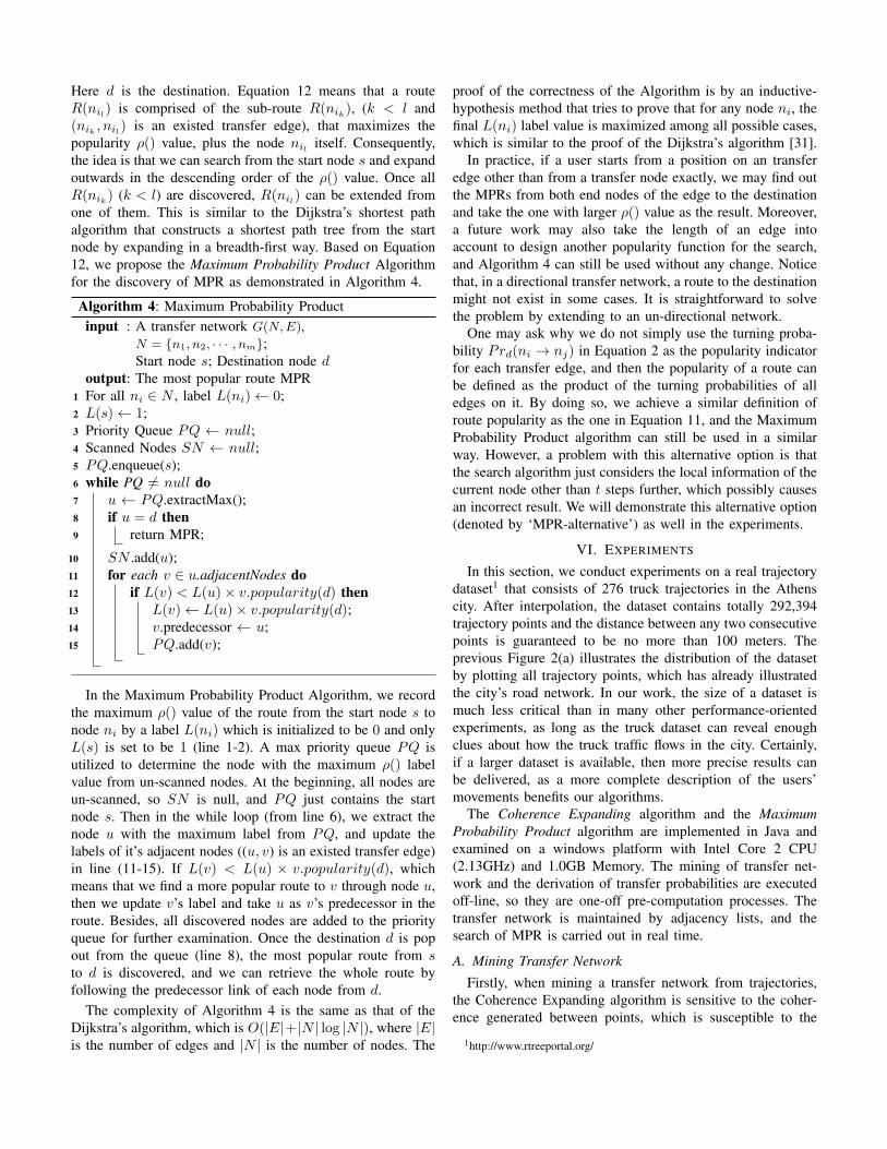
Fig. 6. Illustration of Example Queries (Start Node: 𝐴, End Node: 𝐵)

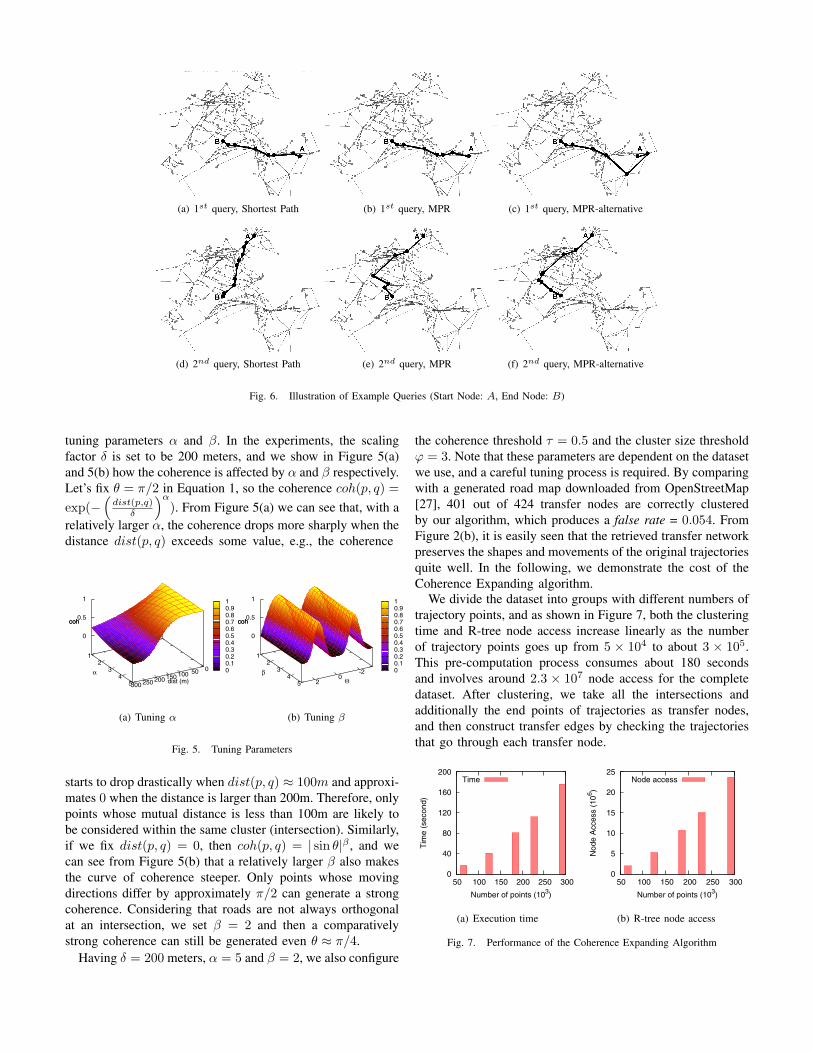
tuning parameters 𝛼 and 𝛽. In the experiments, the scalingfactor 𝛿 is set to be 200 meters, and we show in Figure 5(a)and 5(b) how the coherence is affected by 𝛼 and 𝛽 respectively.Let’s fix 𝜃 = 𝜋/2 in Equation 1, so the coherence 𝑐𝑜ℎ(𝑝, 𝑞) =

exp(−(

𝑑𝑖𝑠𝑡(𝑝,𝑞)𝛿

)𝛼

). From Figure 5(a) we can see that, with arelatively larger 𝛼, the coherence drops more sharply when thedistance 𝑑𝑖𝑠𝑡(𝑝, 𝑞) exceeds some value, e.g., the coherence

0 0.1 0.2 0.3 0.4 0.5 0.6 0.7 0.8 0.9 1

0 50 100 150 200 250 300

1 2

3 4

5

0

0.5

1

coh

dist (m)α

coh

(a) Tuning 𝛼

0 0.1 0.2 0.3 0.4 0.5 0.6 0.7 0.8 0.9 1

-2 0

2

1 2

3 4

5

0

0.5

1

coh

Θβ

coh

(b) Tuning 𝛽

Fig. 5. Tuning Parameters

starts to drop drastically when 𝑑𝑖𝑠𝑡(𝑝, 𝑞) ≈ 100𝑚 and approxi-mates 0 when the distance is larger than 200m. Therefore, onlypoints whose mutual distance is less than 100m are likely tobe considered within the same cluster (intersection). Similarly,if we fix 𝑑𝑖𝑠𝑡(𝑝, 𝑞) = 0, then 𝑐𝑜ℎ(𝑝, 𝑞) = ∣ sin 𝜃∣𝛽 , and wecan see from Figure 5(b) that a relatively larger 𝛽 also makesthe curve of coherence steeper. Only points whose movingdirections differ by approximately 𝜋/2 can generate a strongcoherence. Considering that roads are not always orthogonalat an intersection, we set 𝛽 = 2 and then a comparativelystrong coherence can still be generated even 𝜃 ≈ 𝜋/4.

Having 𝛿 = 200 meters, 𝛼 = 5 and 𝛽 = 2, we also configure

the coherence threshold 𝜏 = 0.5 and the cluster size threshold𝜑 = 3. Note that these parameters are dependent on the datasetwe use, and a careful tuning process is required. By comparingwith a generated road map downloaded from OpenStreetMap[27], 401 out of 424 transfer nodes are correctly clusteredby our algorithm, which produces a false rate = 0.054. FromFigure 2(b), it is easily seen that the retrieved transfer networkpreserves the shapes and movements of the original trajectoriesquite well. In the following, we demonstrate the cost of theCoherence Expanding algorithm.

We divide the dataset into groups with different numbers oftrajectory points, and as shown in Figure 7, both the clusteringtime and R-tree node access increase linearly as the numberof trajectory points goes up from 5 × 104 to about 3 × 105.This pre-computation process consumes about 180 secondsand involves around 2.3 × 107 node access for the completedataset. After clustering, we take all the intersections andadditionally the end points of trajectories as transfer nodes,and then construct transfer edges by checking the trajectoriesthat go through each transfer node.

0

40

80

120

160

200

50 100 150 200 250 300

Tim

e (s

econ

d)

Number of points (103)

Time

(a) Execution time

0

5

10

15

20

25

50 100 150 200 250 300

Nod

e A

cces

s (1

06 )

Number of points (103)

Node access

(b) R-tree node access

Fig. 7. Performance of the Coherence Expanding Algorithm

0

2

4

6

8

10

12

14

4 6 8 10 12

Num

ber

of N

odes

Length of SP

Shortest PathMPR

MPR-alternative

(a)

0

5000

10000

15000

20000

25000

4 6 8 10 12

Dis

tanc

e (m

eter

)

Length of SP

Shortest PathMPR

MPR-alternative

(b)

0

30

60

90

120

150

4 6 8 10 12

Que

ry T

ime

(ms)

Length of SP

Shortest PathMPR

MPR-alternative

(c)

0

30

60

90

120

150

4 6 8 10 12

Num

ber

of V

isite

d N

odes

Length of SP

Shortest PathMPR

MPR-alternative

(d)

Fig. 8. The Shortest Path vs. The MPR

B. Deriving Transfer Probability

For figuring out the transfer probability and derive the vector𝑉 (see Equation 10) for each of the transfer nodes, we firstof all calculate the transition probability w.r.t. each node byEquation 5. Here we simply enumerate every trajectory thatgoes through a transfer node and compute the probability byEquation 2. Then we acquire the transition matrix 𝑃 for eachtransfer node, and the calculation of vector 𝑉 in Equation 10is conducted using Matlab off-line. After that, we attach thetransfer probabilities in 𝑉 as indicators to the correspondingtransfer nodes. The details of this part are skipped as the matrixoperations involved here are straightforward.

C. Illustration of the MPR

In the following, we illustrate the search results of ourMaximum Probability Product algorithm and compare theresults with the corresponding shortest paths using two ex-ample queries, and study the average performance of thealgorithms. Additionally, we demonstrate the search results ofthe alternative solution mentioned in subsection V, in whichthe turning probability defined in Equation 2 is used as thepopularity indicator, and we show that this simple alternativeoption may lead to not accurate enough results. Notice that the‘goodness’ of a search result is hard to be measured by someground truth, and here we just present the results virtuallyfrom which we can have an intuitive impression.

Let’s denote the search output of our algorithm by ‘MPR’,the result of the alternative solution by ‘MPR-alternative’,and the shortest path by ‘shortest path’. In the first examplequery, the most popular route (Figure 6(b)) is almost thesame as the corresponding shortest path (Figure 6(a)), wherethe destination is drawn as a rectangle. However, if we usethe alternative solution for finding a popular route, it leadsto a route that moves oppositely in the beginning and thenwinds around to the destination as shown in Figure 6(c),which is intuitively not a good choice for truck deliveries.Consequently, we would say this alternative solution may failto find a globally popular route as it looks at the turningprobabilities of the immediately adjacent edges only, whileour algorithm further considers 𝑡 steps forward. Nevertheless,in many other cases, the MPR and the MPR-alternative maystill be very similar, as we can see in Figure 6(e) and Figure6(f) that are the results of the second example query.

Even though the MPR and the corresponding shortest pathare nearly the same in the first query, we can still find a lotscenarios that the MPR is very different from the shortestpath since drivers may not always follow the shortest pathfor truck deliveries. An example is in Figure 6(e) wherethe MPR deviates to the left, while the shortest path goesstraight down to the destination in Figure 6(d). To explainthis phenomenon, we may have a look at how trajectoriesconnect to the destination exactly. Figure 9(a) depicts all thetrajectories that go to the destination 𝐵, and the summary ofthe trajectory distribution is shown in Figure 9(b). There aretotally 14 trajectories go to the destination from the left partwhile only 2 trajectories go straight down to the destination.Therefore, more truck drivers prefer the route through the leftpart and that is the reason why the MPR and also the MPR-alternative are found out to follow a different way from theshortest path. Furthermore, this example demonstrates that apreferable MPR is not necessarily to be the shortest path.

B

(a) Trajectories

\

14

2

3

7B

(b) Summary

Fig. 9. Statistics of Trajectories

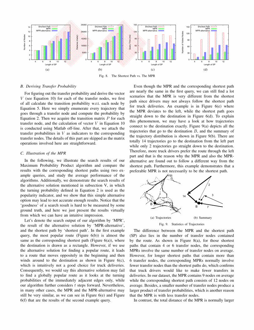
The difference between the MPR and the shortest path(SP) also lies in the number of transfer nodes containedby the route. As shown in Figure 8(a), for those shortestpaths that contain 4 or 6 transfer nodes, the correspondingMPRs involve the same number of transfer nodes on average.However, for longer shortest paths that contain more than6 transfer nodes, the corresponding MPRs normally involvefewer transfer nodes than the shortest paths do, which confirmsthat truck drivers would like to make fewer transfers indeliveries. In our dataset, the MPR contains 9 nodes on averagewhile the corresponding shortest path consists of 12 nodes onaverage. Besides, a smaller number of transfer nodes produce alarger product of transfer probabilities, which is another reasonthat the MPR is with less transfer nodes.

In contrast, the total distance of the MPR is normally larger

than that of the corresponding shortest path as illustrated inFigure 8(b). Compared to a shortest path that contains 12nodes and with a length of 18km, the corresponding MPRis about 1/4 longer on average, which implies the fact thatthe shortest path is not always the most favorite one anddrivers may take a slightly longer route in order to usehigher quality roads, or to avoid traffic, or to maximizedelivery efficiency, etc. Importantly, the driver behaviors canbe partially discovered by searching the most popular routes.

D. The Efficiency of Searching the MPR

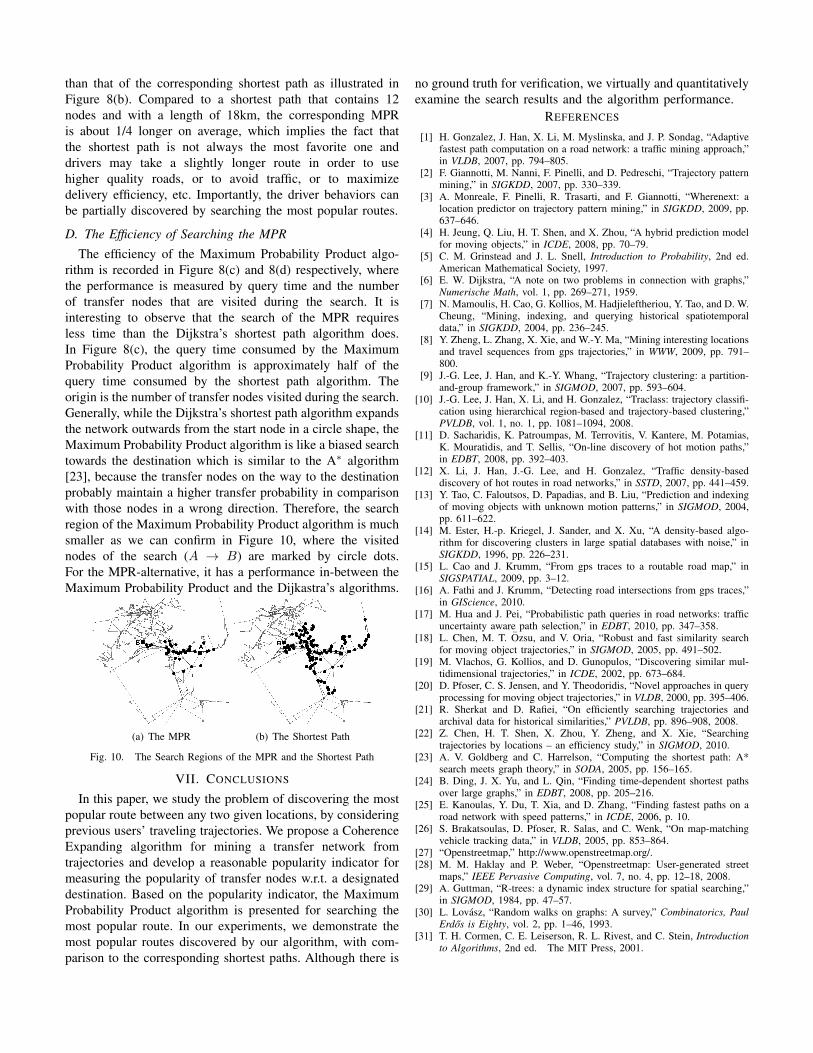
The efficiency of the Maximum Probability Product algo-rithm is recorded in Figure 8(c) and 8(d) respectively, wherethe performance is measured by query time and the numberof transfer nodes that are visited during the search. It isinteresting to observe that the search of the MPR requiresless time than the Dijkstra’s shortest path algorithm does.In Figure 8(c), the query time consumed by the MaximumProbability Product algorithm is approximately half of thequery time consumed by the shortest path algorithm. Theorigin is the number of transfer nodes visited during the search.Generally, while the Dijkstra’s shortest path algorithm expandsthe network outwards from the start node in a circle shape, theMaximum Probability Product algorithm is like a biased searchtowards the destination which is similar to the A∗ algorithm[23], because the transfer nodes on the way to the destinationprobably maintain a higher transfer probability in comparisonwith those nodes in a wrong direction. Therefore, the searchregion of the Maximum Probability Product algorithm is muchsmaller as we can confirm in Figure 10, where the visitednodes of the search (𝐴 → 𝐵) are marked by circle dots.For the MPR-alternative, it has a performance in-between theMaximum Probability Product and the Dijkastra’s algorithms.

(a) The MPR (b) The Shortest Path

Fig. 10. The Search Regions of the MPR and the Shortest Path

VII. CONCLUSIONS

In this paper, we study the problem of discovering the mostpopular route between any two given locations, by consideringprevious users’ traveling trajectories. We propose a CoherenceExpanding algorithm for mining a transfer network fromtrajectories and develop a reasonable popularity indicator formeasuring the popularity of transfer nodes w.r.t. a designateddestination. Based on the popularity indicator, the MaximumProbability Product algorithm is presented for searching themost popular route. In our experiments, we demonstrate themost popular routes discovered by our algorithm, with com-parison to the corresponding shortest paths. Although there is

no ground truth for verification, we virtually and quantitativelyexamine the search results and the algorithm performance.

REFERENCES

[1] H. Gonzalez, J. Han, X. Li, M. Myslinska, and J. P. Sondag, “Adaptivefastest path computation on a road network: a traffic mining approach,”in VLDB, 2007, pp. 794–805.

[2] F. Giannotti, M. Nanni, F. Pinelli, and D. Pedreschi, “Trajectory patternmining,” in SIGKDD, 2007, pp. 330–339.

[3] A. Monreale, F. Pinelli, R. Trasarti, and F. Giannotti, “Wherenext: alocation predictor on trajectory pattern mining,” in SIGKDD, 2009, pp.637–646.

[4] H. Jeung, Q. Liu, H. T. Shen, and X. Zhou, “A hybrid prediction modelfor moving objects,” in ICDE, 2008, pp. 70–79.

[5] C. M. Grinstead and J. L. Snell, Introduction to Probability, 2nd ed.American Mathematical Society, 1997.

[6] E. W. Dijkstra, “A note on two problems in connection with graphs,”Numerische Math, vol. 1, pp. 269–271, 1959.

[7] N. Mamoulis, H. Cao, G. Kollios, M. Hadjieleftheriou, Y. Tao, and D. W.Cheung, “Mining, indexing, and querying historical spatiotemporaldata,” in SIGKDD, 2004, pp. 236–245.

[8] Y. Zheng, L. Zhang, X. Xie, and W.-Y. Ma, “Mining interesting locationsand travel sequences from gps trajectories,” in WWW, 2009, pp. 791–800.

[9] J.-G. Lee, J. Han, and K.-Y. Whang, “Trajectory clustering: a partition-and-group framework,” in SIGMOD, 2007, pp. 593–604.

[10] J.-G. Lee, J. Han, X. Li, and H. Gonzalez, “Traclass: trajectory classifi-cation using hierarchical region-based and trajectory-based clustering,”PVLDB, vol. 1, no. 1, pp. 1081–1094, 2008.

[11] D. Sacharidis, K. Patroumpas, M. Terrovitis, V. Kantere, M. Potamias,K. Mouratidis, and T. Sellis, “On-line discovery of hot motion paths,”in EDBT, 2008, pp. 392–403.

[12] X. Li, J. Han, J.-G. Lee, and H. Gonzalez, “Traffic density-baseddiscovery of hot routes in road networks,” in SSTD, 2007, pp. 441–459.

[13] Y. Tao, C. Faloutsos, D. Papadias, and B. Liu, “Prediction and indexingof moving objects with unknown motion patterns,” in SIGMOD, 2004,pp. 611–622.

[14] M. Ester, H.-p. Kriegel, J. Sander, and X. Xu, “A density-based algo-rithm for discovering clusters in large spatial databases with noise,” inSIGKDD, 1996, pp. 226–231.

[15] L. Cao and J. Krumm, “From gps traces to a routable road map,” inSIGSPATIAL, 2009, pp. 3–12.

[16] A. Fathi and J. Krumm, “Detecting road intersections from gps traces,”in GIScience, 2010.

[17] M. Hua and J. Pei, “Probabilistic path queries in road networks: trafficuncertainty aware path selection,” in EDBT, 2010, pp. 347–358.

[18] L. Chen, M. T. Ozsu, and V. Oria, “Robust and fast similarity searchfor moving object trajectories,” in SIGMOD, 2005, pp. 491–502.

[19] M. Vlachos, G. Kollios, and D. Gunopulos, “Discovering similar mul-tidimensional trajectories,” in ICDE, 2002, pp. 673–684.

[20] D. Pfoser, C. S. Jensen, and Y. Theodoridis, “Novel approaches in queryprocessing for moving object trajectories,” in VLDB, 2000, pp. 395–406.

[21] R. Sherkat and D. Rafiei, “On efficiently searching trajectories andarchival data for historical similarities,” PVLDB, pp. 896–908, 2008.

[22] Z. Chen, H. T. Shen, X. Zhou, Y. Zheng, and X. Xie, “Searchingtrajectories by locations – an efficiency study,” in SIGMOD, 2010.

[23] A. V. Goldberg and C. Harrelson, “Computing the shortest path: A*search meets graph theory,” in SODA, 2005, pp. 156–165.

[24] B. Ding, J. X. Yu, and L. Qin, “Finding time-dependent shortest pathsover large graphs,” in EDBT, 2008, pp. 205–216.

[25] E. Kanoulas, Y. Du, T. Xia, and D. Zhang, “Finding fastest paths on aroad network with speed patterns,” in ICDE, 2006, p. 10.

[26] S. Brakatsoulas, D. Pfoser, R. Salas, and C. Wenk, “On map-matchingvehicle tracking data,” in VLDB, 2005, pp. 853–864.

[27] “Openstreetmap,” http://www.openstreetmap.org/.[28] M. M. Haklay and P. Weber, “Openstreetmap: User-generated street

maps,” IEEE Pervasive Computing, vol. 7, no. 4, pp. 12–18, 2008.[29] A. Guttman, “R-trees: a dynamic index structure for spatial searching,”

in SIGMOD, 1984, pp. 47–57.[30] L. Lovasz, “Random walks on graphs: A survey,” Combinatorics, Paul

Erdos is Eighty, vol. 2, pp. 1–46, 1993.[31] T. H. Cormen, C. E. Leiserson, R. L. Rivest, and C. Stein, Introduction

to Algorithms, 2nd ed. The MIT Press, 2001.