31
Computer Science, Informatik 4 Communication and Distributed Systems Simulation “Discrete-Event System Simulation” Dr. Mesut Güneş

Computer Science, Informatik 4 Communication and Distributed Systems
Simulation
“Discrete-Event System Simulation”
Dr. Mesut Güneş

Computer Science, Informatik 4 Communication and Distributed Systems
Chapter 6
Random-Variate Generation
Dr. Mesut Güneş
Computer Science, Informatik 4 Communication and Distributed Systems
3Chapter 6. Random-Variate Generation
Purpose & Overview
Develop understanding of generating samples from a specified distribution as input to a simulation model.
Illustrate some widely-used techniques for generating random variates.• Inverse-transform technique• Acceptance-rejection technique• Special properties

Dr. Mesut Güneş
Computer Science, Informatik 4 Communication and Distributed Systems
4Chapter 6. Random-Variate Generation
Preparation
It is assumed that a source of uniform [0,1] random numbers exists.• Linear Congruential Method
Random numbers R, R1, R2, … with• PDF
• CDF
⎩⎨⎧ ≤≤
=otherwise0
101)(
xxfR
⎪⎩
⎪⎨
⎧
>≤≤
<=
1110
00)(
xxx
xxFR

Dr. Mesut Güneş
Computer Science, Informatik 4 Communication and Distributed Systems
5Chapter 6. Random-Variate Generation
Inverse-transform Technique
The concept:• For CDF function: r = F(x)• Generate r from uniform (0,1), a.k.a U(0,1)• Find x,
x = F-1(r)
r1
x1
r = F(x)
x
F(x)
1
r1
x1
r = F(x)
x
F(x)
1

Dr. Mesut Güneş
Computer Science, Informatik 4 Communication and Distributed Systems
6Chapter 6. Random-Variate Generation
Inverse-transform Technique
The inverse-transform technique can be used in principle for any distribution.Most useful when the CDF F(x) has an inverse F -1(x) which is easy to compute.
Required steps1. Compute the CDF of the desired random variable X.2. Set F(X)=R on the range of X.3. Solve the equation F(X)=R for X in terms of R.4. Generate uniform random numbers R1, R2, R3, … and compute
the desired random variate by Xi = F-1(Ri)

Dr. Mesut Güneş
Computer Science, Informatik 4 Communication and Distributed Systems
7Chapter 6. Random-Variate Generation
Exponential Distribution
Exponential Distribution• PDF
• CDF
To generate X1, X2, X3 …
xexf λλ −=)(
xexF λ−−=1)(
)(
)1ln(
)1ln()1ln(
11
1 RFX
RX
RX
RXRe
ReX
X
−
−
−
=
−−=
−−
=
−=−−=
=−
λ
λ
λ
λ
λ
Simplification
• Since R and (1-R) are uniformly distributed on [0,1]
λ)ln(RX −=

Dr. Mesut Güneş
Computer Science, Informatik 4 Communication and Distributed Systems
8Chapter 6. Random-Variate Generation
Exponential Distribution
Figure: Inverse-transform technique for exp(λ = 1)

Dr. Mesut Güneş
Computer Science, Informatik 4 Communication and Distributed Systems
9Chapter 6. Random-Variate Generation
Example: Generate 200 variates Xi with distribution exp(λ= 1)• Generate 200 Rs with U(0,1), the histogram of Xs become:
• Check: Does the random variable X1 have the desired distribution?
Exponential Distribution
)())(()( 00101 xFxFRPxXP =≤=≤
0
0,1
0,2
0,3
0,4
0,5
0,6
0,7
0,5 1 1,5 2 2,5 3 3,5 4 4,5 5 5,5 6 6,5 7
Empirical Histogram Theor. PDF
Dr. Mesut Güneş
Computer Science, Informatik 4 Communication and Distributed Systems
10Chapter 6. Random-Variate Generation
Other Distributions
Examples of other distributions for which inverse CDF works are:• Uniform distribution• Weibull distribution• Triangular distribution

Dr. Mesut Güneş
Computer Science, Informatik 4 Communication and Distributed Systems
11Chapter 6. Random-Variate Generation
Uniform Distribution
Random variable X uniformly distributed over [a, b]
)()(
)(
abRaXabRaX
RabaX
RXF
−+=−=−
=−−
=

Dr. Mesut Güneş
Computer Science, Informatik 4 Communication and Distributed Systems
12Chapter 6. Random-Variate Generation
Weibull Distribution
The Weibull Distribution is described by
• CDF
The variate is
( )βαx
eXF −−=1)(
( )
( )
( )
β
β β
ββ
β
β
βα
α
α
αα
βα
βα
)1ln(
)1ln(
)1ln(
)1ln(
)1ln(
1
1
)(
RX
Rx
RX
RX
R
Re
Re
RXF
X
X
X
−−⋅=
−⋅−=
−⋅−=
−−=
−=−
−=
=−
=
−
−
( )βαββαβ x
exxf −−= 1)(

Dr. Mesut Güneş
Computer Science, Informatik 4 Communication and Distributed Systems
13Chapter 6. Random-Variate Generation
Triangular Distribution
The CDF of a Triangular Distribution with endpoints (0, 2) is given by
X is generated by2
)2(1
21for and2
10For
2
2
XR
X
XR
X
−−=
≤≤
=
≤≤
⎪⎪⎪
⎩
⎪⎪⎪
⎨
⎧
>
≤<−
−
≤<
≤
=
21
212
)2(1
102
00
)( 2
2
x
xx
xxx
xF
⎪⎩
⎪⎨⎧
≤<−−≤≤
=1)1(22
02
21
21
RRRR
X
Dr. Mesut Güneş
Computer Science, Informatik 4 Communication and Distributed Systems
14Chapter 6. Random-Variate Generation
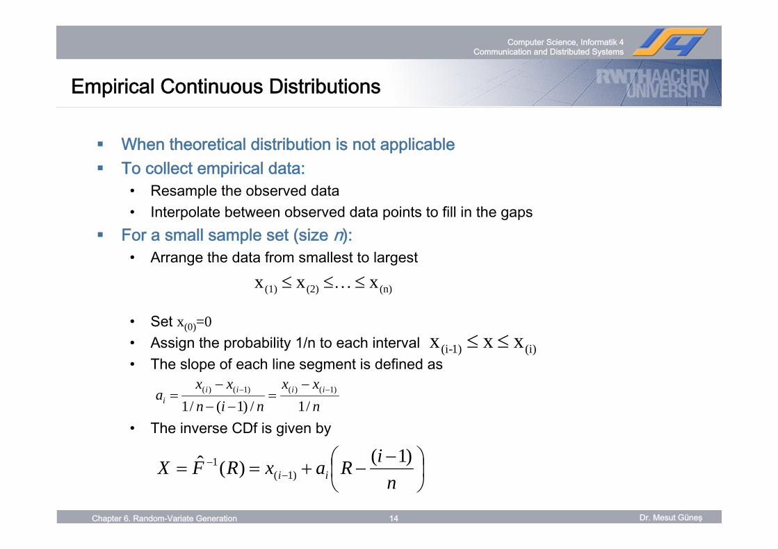
Empirical Continuous Distributions
When theoretical distribution is not applicableTo collect empirical data:
• Resample the observed data• Interpolate between observed data points to fill in the gaps
For a small sample set (size n):• Arrange the data from smallest to largest
• Set x(0)=0• Assign the probability 1/n to each interval • The slope of each line segment is defined as
• The inverse CDf is given by
(n)(2)(1) x x x ≤…≤≤
(i)1)-(i x x x ≤≤
⎟⎠⎞
⎜⎝⎛ −
−+== −−
niRaxRFX ii
)1()(ˆ)1(
1
nxx
ninxx
a iiiii /1/)1(/1
)1()()1()( −− −=
−−
−=

Dr. Mesut Güneş
Computer Science, Informatik 4 Communication and Distributed Systems
15Chapter 6. Random-Variate Generation
Empirical Continuous Distributions
4.651.00.21.83 < x ≤2.765
1.900.80.21.45 < x ≤ 1.834
1.050.60.21.24 < x ≤ 1.453
2.200.40.20.8 < x ≤ 1.242
4.000.20.20.0 < x ≤ 0.81
Slope aiCumulative ProbabilityProbabilityIntervali
66.1)6.071.0(90.145.1
)/)14((71.0
14)14(1
1
=−+=
−−+==
− nRaxXR

Dr. Mesut Güneş
Computer Science, Informatik 4 Communication and Distributed Systems
16Chapter 6. Random-Variate Generation
Empirical Continuous Distributions
What happens for large samples of data• Several hundreds or tens of thousand
First summarize the data into a frequency distribution with smaller number of intervalsAfterwards, fit continuous empirical CDF to the frequency distributionSlight modifications• Slope
• The inverse CDf is given by
1
)1()(
−
−
−
−=
ii
iii cc
xxa
( )1)1(1 )(ˆ
−−− −+== iii cRaxRFX
ci cumulative probability of the first i intervals

Dr. Mesut Güneş
Computer Science, Informatik 4 Communication and Distributed Systems
17Chapter 6. Random-Variate Generation
Empirical Continuous Distributions
Example: Suppose the data collected for 100 broken-widget repair times are:
iInterval (Hours) Frequency
Relative Frequency
Cumulative Frequency, c i
Slope, a i
1 0.25 ≤ x ≤ 0.5 31 0.31 0.31 0.812 0.5 ≤ x ≤ 1.0 10 0.10 0.41 5.03 1.0 ≤ x ≤ 1.5 25 0.25 0.66 2.04 1.5 ≤ x ≤ 2.0 34 0.34 1.00 1.47
Consider R1 = 0.83:
c3 = 0.66 < R1 < c4 = 1.00
X1 = x(4-1) + a4(R1 – c(4-1))= 1.5 + 1.47(0.83-0.66)= 1.75
Dr. Mesut Güneş
Computer Science, Informatik 4 Communication and Distributed Systems
18Chapter 6. Random-Variate Generation
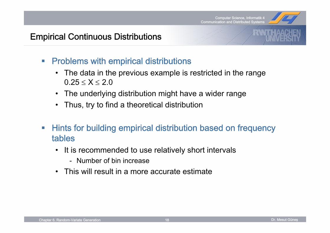
Empirical Continuous Distributions
Problems with empirical distributions• The data in the previous example is restricted in the range
0.25 ≤ X ≤ 2.0• The underlying distribution might have a wider range• Thus, try to find a theoretical distribution
Hints for building empirical distribution based on frequency tables• It is recommended to use relatively short intervals
- Number of bin increase• This will result in a more accurate estimate

Dr. Mesut Güneş
Computer Science, Informatik 4 Communication and Distributed Systems
19Chapter 6. Random-Variate Generation
Discrete Distribution
All discrete distributions can be generated via inverse-transform techniqueMethod: numerically, table-lookup procedure, algebraically, or a formulaExamples of application:• Empirical• Discrete uniform• Gamma
Dr. Mesut Güneş
Computer Science, Informatik 4 Communication and Distributed Systems
20Chapter 6. Random-Variate Generation
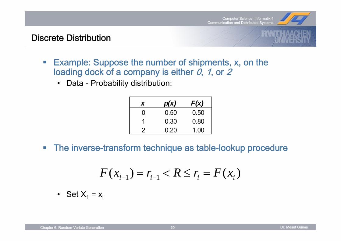
Discrete Distribution
Example: Suppose the number of shipments, x, on the loading dock of a company is either 0, 1, or 2• Data - Probability distribution:
The inverse-transform technique as table-lookup procedure
• Set X1 = xi
x p(x) F(x)0 0.50 0.501 0.30 0.802 0.20 1.00
)()( 11 iiii xFrRrxF =≤<= −−

Dr. Mesut Güneş
Computer Science, Informatik 4 Communication and Distributed Systems
21Chapter 6. Random-Variate Generation
Discrete Distribution
Consider R1 = 0.73:F(xi-1) < R <= F(xi)F(x0) < 0.73 <= F(x1)
Hence, x1 = 1
0.18.08.05.0
5.0
,2,1,0
≤<≤<
≤
⎪⎩
⎪⎨
⎧=
RR
Rx
Method - Given R, the generation scheme becomes:
21.0310.8200.51
Output xiInput rii
Table for generating the discrete variate
X

Dr. Mesut Güneş
Computer Science, Informatik 4 Communication and Distributed Systems
22Chapter 6. Random-Variate Generation
Acceptance-Rejection technique
Useful particularly when inverse cdf does not exist in closed form, a.k.a. thinningIllustration: To generate random variates, X ~ U(1/4, 1)
R does not have the desired distribution, but R conditioned (R’) on the event {R ≥ ¼} does.Efficiency: Depends heavily on the ability to minimize the number of rejections.
Procedures:Step 1. Generate R ~ U[0,1]Step 2a. If R >= ¼, accept X=R.Step 2b. If R < ¼, reject R, return
to Step 1
Generate R
Condition
Output R’
yes
no

Dr. Mesut Güneş
Computer Science, Informatik 4 Communication and Distributed Systems
23Chapter 6. Random-Variate Generation
Poisson Distribution
PMF of a Poisson Distribution
Exactly n arrivals during one time unit
Since interarrival times are exponentially distributed we can set
• Well known, we derived this generator in the beginning of the class
αα −== en
nNPn
!)(
12121 1 +++++<≤+++ nnn AAAAAAA LL
α)ln( i
iRA −
=

Dr. Mesut Güneş
Computer Science, Informatik 4 Communication and Distributed Systems
24Chapter 6. Random-Variate Generation
Poisson Distribution
Substitute the sum by
Simplify by• multiply by -α, which reverses the inequality sign• sum of logs is the log of a product
Simplify by eln(x) = x
∏∏+
=
−
=
>≥1
11
n
ii
n
ii ReR α
∑∑+
==
−<≤
− 1
11
)ln(1)ln( n
i
in
i
i RRαα
∏∑∑∏=
+
===
=>−≥=n
ii
n
ii
n
ii
n
ii RRRR
1
1
111
ln)ln()ln(ln α

Dr. Mesut Güneş
Computer Science, Informatik 4 Communication and Distributed Systems
25Chapter 6. Random-Variate Generation
Poisson Distribution
Procedure of generating a Poisson random variate N is as follows1. Set n=0, P=12. Generate a random number Rn+1, and replace P by P x Rn+1
3. If P < exp(-α), then accept N=n- Otherwise, reject the current n, increase n by one, and return to
step 2.

Dr. Mesut Güneş
Computer Science, Informatik 4 Communication and Distributed Systems
26Chapter 6. Random-Variate Generation
Poisson Distribution
Example: Generate three Poisson variates with mean α=0.2• exp(-0.2) = 0.8187
Variate 1• Step 1: Set n=0, P=1• Step 2: R1 = 0.4357, P = 1 x 0.4357• Step 3: Since P = 0.4357 < exp(- 0.2), accept N = 0
Variate 2• Step 1: Set n=0, P=1• Step 2: R1 = 0.4146, P = 1 x 0.4146• Step 3: Since P = 0.4146 < exp(-0.2), accept N = 0
Variate 3• Step 1: Set n=0, P=1• Step 2: R1 = 0.8353, P = 1 x 0.8353• Step 3: Since P= 0.8353 > exp(-0.2), reject n=0 and return to Step 2 with n=1• Step 2: R2 = 0.9952, P = 0.8353 x 0.9952 = 0.8313• Step 3: Since P= 0.8313 > exp(-0.2), reject n=1 and return to Step 2 with n=2• Step 2: R3 = 0.8004, P = 0.8313 x 0.8004 = 0.6654• Step 3: Since P = 0.6654 < exp(-0.2), accept N = 2
Dr. Mesut Güneş
Computer Science, Informatik 4 Communication and Distributed Systems
27Chapter 6. Random-Variate Generation
Poisson Distribution
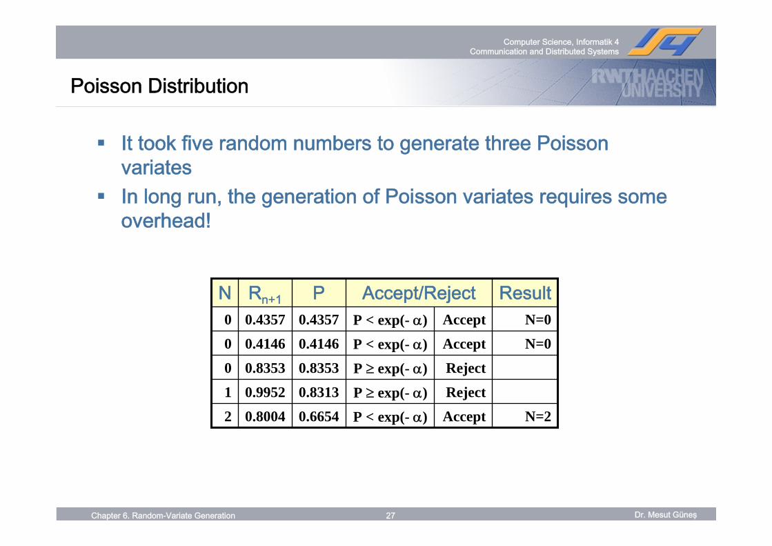
It took five random numbers to generate three Poisson variatesIn long run, the generation of Poisson variates requires some overhead!
N=2AcceptP < exp(- α)0.66540.80042
RejectP ≥ exp(- α)0.83130.99521
RejectP ≥ exp(- α)0.83530.83530
N=0AcceptP < exp(- α)0.41460.41460
N=0AcceptP < exp(- α)0.43570.43570
ResultAccept/RejectPRn+1N

Dr. Mesut Güneş
Computer Science, Informatik 4 Communication and Distributed Systems
28Chapter 6. Random-Variate Generation
Special Properties
Based on features of particular family of probability distributionsFor example:• Direct Transformation for normal and lognormal distributions• Convolution• Beta distribution (from gamma distribution)

Dr. Mesut Güneş
Computer Science, Informatik 4 Communication and Distributed Systems
29Chapter 6. Random-Variate Generation
Approach for N(0,1):• Consider two standard normal random variables, Z1 and Z2, plotted as a
point in the plane:
• B2 = Z21 + Z2
2 ~ χ2 distribution with 2 degrees of freedom = Exp(λ = 2). Hence,
• The radius B and angle φ are mutually independent.
Direct Transformation
2/1)ln2( RB −=
In polar coordinates:Z1 = B cos(φ)Z2 = B sin(φ)
)2sin()ln2(
)2cos()ln2(
22/1
2
22/1
1
RRZ
RRZ
π
π
−=
−=

Dr. Mesut Güneş
Computer Science, Informatik 4 Communication and Distributed Systems
30Chapter 6. Random-Variate Generation
Direct Transformation
Approach for N(μ,σ2):• Generate Zi ~ N(0,1)
Approach for Lognormal(μ,σ2):• Generate X ~ N((μ,σ2)
Yi = eXi
Xi = μ + σ Zi

Dr. Mesut Güneş
Computer Science, Informatik 4 Communication and Distributed Systems
31Chapter 6. Random-Variate Generation
Summary
Principles of random-variate generation via• Inverse-transform technique• Acceptance-rejection technique• Special properties
Important for generating continuous and discrete distributions


