Discrete Multiscale Vector Field Decomposition Yiying Tong USC Santiago Lombeyda Caltech Anil N. Hirani Caltech Mathieu Desbrun USC Figure 1: Decomposing Vector Fields: the tangential component of a wind field interacting with an ear (left, LIC visualization [ 5]) reveals its curl free component (middle) and divergence-free component (right) after decomposition. In this paper, simple computational tools are introduced to produce such a decomposition, for discrete 2D and 3D vector fields defined on irregular grids,even on curved manifolds. Abstract While 2D and 3D vector fields are ubiquitous in computational sci- ences, their use in graphics is often limited to regular grids, where computations are easily handled through finite-difference methods. In this paper, we propose a set of simple and accurate tools for the analysis of 3D discrete vector fields on arbitrary tetrahedral grids. We introduce a variational, multiscale decomposition of vec- tor fields into three intuitive components: a divergence-free part, a curl-free part, and a harmonic part. We show how our discrete ap- proach matches its well-known smooth analog, called the Helmotz- Hodge decomposition, and that the resulting computational tools have very intuitive geometric interpretation. We demonstrate the versatility of these tools in a series of applications, ranging from data visualization to fluid and deformable object simulation. Keywords: Vector fields, Variational approaches, Hodge decom- position, Scale-space description, Animation, Visualization 1 Introduction Discrete multivalued fields such as vector and tensor fields are ubiq- uitous in computational sciences. In Computer Graphics, they are used in a large number of applications ranging from fluid and de- formable object simulation to the analysis of MRI data for medical prognosis. Due to the sheer complexity of these nonscalar fields, their numerical processing is most often performed on regular grids, due to a lack of simple and accurate tools for irregular grids. Yet, arbitrary grids are more efficient and flexible at discretizing 2D and 3D regions, whether they are in Euclidean spaces or on curved man- ifolds. The goal of this paper is to present a simple and accurate approach to vector field processing on arbitrary tetrahedral grids, to catalyze the development of algorithms and implementations of such rich data in computer graphics. Most of the work done so far on discrete vector field analysis has tried to mimic well-known differential properties of vector fields dating back to Poincar´ e (1854-1912). Globus et al. [ 11] for instance described a methodology for vector field analysis by examining the eigenvalues of the jacobian matrix of a velocity field trilinearly in- terpolated on curvilinear grids. They also created a discrete topol- ogy of vector fields by connecting critical points through stream- lines. This notion of topology can be used to not only analyze, but also to describe vector fields, even noisy ones that can be smoothed while preserving [29] or simplifying [27, 14] their topology. An al- ternative for computing the singularities of three dimensional flow fields was shown in [16] using Clifford algebra. It can not only find and classify point singularities, but also line and surface singulari- ties. However, the approach is so far restricted to regular grid data; moreover, the computations involved provide topological informa- tion only, and often return false positives. This is actually a com- mon problem: since most vector field feature detections are based on very local estimates (often using the jacobian or the winding number), inevitable noise in the data often leads to poor numerical quality of the approximants, and thus inaccurate feature detection. As we will see, we use instead a variational approach to offer a more global solution to feature detection that does not suffer from such sensitivity to noise. Smoothing vector fields has also been proposed as an efficient way to simplify complex datasets, and render the analysis more tractable [29, 4]: for instance, [24, 9] use anisotropic nonlinear dif- fusion methods to clean “noise” (small-scale features) from 2D and 3D fluid flows. This general idea is essential when dealing with very complex data sets issued from large simulation on supercom- puters: the native resolution of the data prevents any global pro- cessing without prior simplification. We will also provide, in con- junction with a vector field decomposition, a multiscale description of vector fields to allow for a multiresolution probing of the data. 1.1 Hodge Decomposition for Smooth Fields For smooth data, there is a well known way to decompose a vec- tor field into both intuitive and useful components: it is called the Helmholtz-Hodge decomposition [ 1]. First, recall that ∇ = (∂/∂x, ∂/∂y , ∂/∂z) t is the gradient, ∇· = ∂/∂x + ∂/∂y + ∂/∂z is the divergence operator, and ∇ × is the curl operator (also called rota- tional). With this notation, for a smooth 3D vector field ξ defined in a region T , there exists a unique decomposition satisfying the following properties: ξ = ∇u + ∇ ×v + h (1) where: u is a scalar potential field; note that ∇ ×(∇u)= 0, v is a vector potential field; note that ∇ · (∇ ×v)= 0, and 1
Transcript
Discrete Multiscale Vector Field Decomposition
Yiying TongUSC
Santiago LombeydaCaltech
Anil N. HiraniCaltech
Mathieu DesbrunUSC
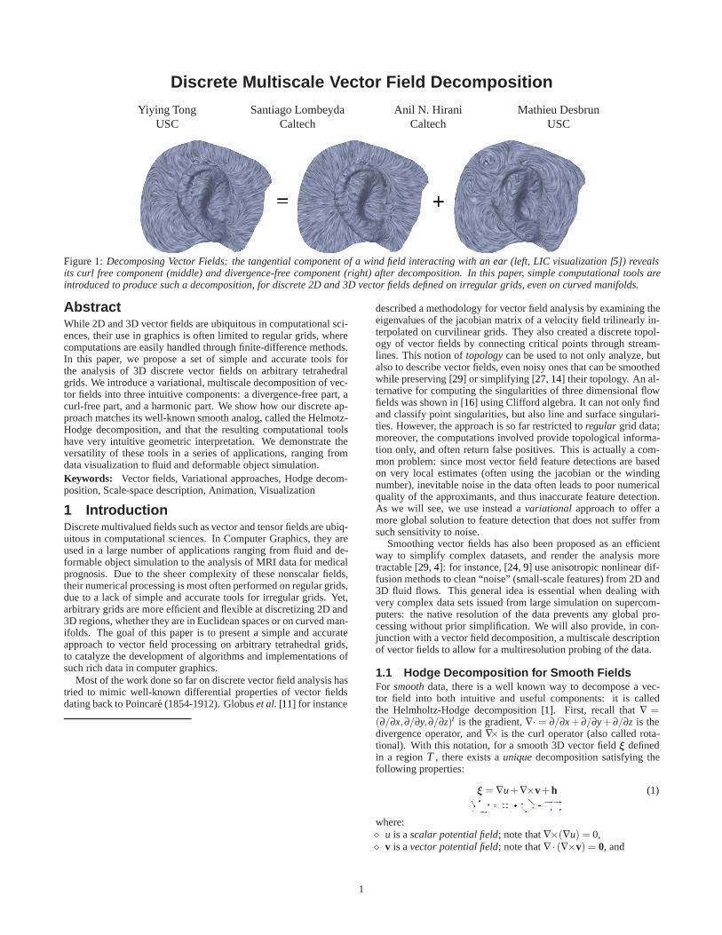
Figure 1: Decomposing Vector Fields: the tangential component of a wind field interacting with an ear (left, LIC visualization [5]) revealsits curl free component (middle) and divergence-free component (right) after decomposition. In this paper, simple computational tools areintroduced to produce such a decomposition, for discrete 2D and 3D vector fields defined on irregular grids, even on curved manifolds.
AbstractWhile 2D and 3D vector fields are ubiquitous in computational sci-ences, their use in graphics is often limited to regular grids, wherecomputations are easily handled through finite-difference methods.In this paper, we propose a set of simple and accurate tools forthe analysis of 3D discrete vector fields on arbitrary tetrahedralgrids. We introduce a variational, multiscale decomposition of vec-tor fields into three intuitive components: a divergence-free part, acurl-free part, and a harmonic part. We show how our discrete ap-proach matches its well-known smooth analog, called the Helmotz-Hodge decomposition, and that the resulting computational toolshave very intuitive geometric interpretation. We demonstrate theversatility of these tools in a series of applications, ranging fromdata visualization to fluid and deformable object simulation.Keywords: Vector fields, Variational approaches, Hodge decom-position, Scale-space description, Animation, Visualization
1 IntroductionDiscrete multivalued fields such as vector and tensor fields are ubiq-uitous in computational sciences. In Computer Graphics, they areused in a large number of applications ranging from fluid and de-formable object simulation to the analysis of MRI data for medicalprognosis. Due to the sheer complexity of these nonscalar fields,their numerical processing is most often performed on regular grids,due to a lack of simple and accurate tools for irregular grids. Yet,arbitrary grids are more efficient and flexible at discretizing 2D and3D regions, whether they are in Euclidean spaces or on curved man-ifolds. The goal of this paper is to present a simple and accurateapproach to vector field processing on arbitrary tetrahedral grids,to catalyze the development of algorithms and implementations ofsuch rich data in computer graphics.
Most of the work done so far on discrete vector field analysis hastried to mimic well-known differential properties of vector fieldsdating back to Poincare (1854-1912). Globus et al. [11] for instance
described a methodology for vector field analysis by examining theeigenvalues of the jacobian matrix of a velocity field trilinearly in-terpolated on curvilinear grids. They also created a discrete topol-ogy of vector fields by connecting critical points through stream-lines. This notion of topology can be used to not only analyze, butalso to describe vector fields, even noisy ones that can be smoothedwhile preserving [29] or simplifying [27, 14] their topology. An al-ternative for computing the singularities of three dimensional flowfields was shown in [16] using Clifford algebra. It can not only findand classify point singularities, but also line and surface singulari-ties. However, the approach is so far restricted to regular grid data;moreover, the computations involved provide topological informa-tion only, and often return false positives. This is actually a com-mon problem: since most vector field feature detections are basedon very local estimates (often using the jacobian or the windingnumber), inevitable noise in the data often leads to poor numericalquality of the approximants, and thus inaccurate feature detection.As we will see, we use instead a variational approach to offer amore global solution to feature detection that does not suffer fromsuch sensitivity to noise.
Smoothing vector fields has also been proposed as an efficientway to simplify complex datasets, and render the analysis moretractable [29, 4]: for instance, [24, 9] use anisotropic nonlinear dif-fusion methods to clean “noise” (small-scale features) from 2D and3D fluid flows. This general idea is essential when dealing withvery complex data sets issued from large simulation on supercom-puters: the native resolution of the data prevents any global pro-cessing without prior simplification. We will also provide, in con-junction with a vector field decomposition, a multiscale descriptionof vector fields to allow for a multiresolution probing of the data.
1.1 Hodge Decomposition for Smooth FieldsFor smooth data, there is a well known way to decompose a vec-tor field into both intuitive and useful components: it is calledthe Helmholtz-Hodge decomposition [1]. First, recall that ∇ =(∂/∂x,∂/∂y,∂/∂z)t is the gradient, ∇· = ∂/∂x +∂/∂y+∂/∂z is thedivergence operator, and ∇× is the curl operator (also called rota-tional). With this notation, for a smooth 3D vector field ξ definedin a region T , there exists a unique decomposition satisfying thefollowing properties:
ξ = ∇u+∇×v+h (1)
where:� u is a scalar potential field; note that ∇×(∇u) = 0,� v is a vector potential field; note that ∇ · (∇×v) = 0, and
1
� h is the so-called ”harmonic” vector field; note that ∇ ·h = 0 and∇×h = 0.
The uniqueness requires proper boundary conditions as well: ∇umust be normal to the boundary ∂T of T , while ∇×v must be tan-gential to it. Due to the properties of the potential fields, ∇u iscalled the curl-free component (∇×(∇u) = 0), while ∇×v is calledthe divergence-free component (∇ · (∇×v) = 0). This decompo-sition is particularly interesting for extraction of the features andsingularities of a flow. For instance, in 2D fields, the curl-free term∇u contains only sources and sinks, while the divergence free term∇×v contains only vortices (see Figure 3). Therefore, in additionto the intrinsic mathematical values of this decomposition, thesecomponents correspond to our intuition about what is a flow.
This natural decomposition is, alas, only well defined for dif-ferential vector fields. One has to extend this smooth definitionto the discrete setting for computational purposes, and this is notrivial matter as even the notion of divergence or curl needs tobe properly defined for discrete data. Discrete Helmholtz-Hodgedecomposition on regular grids has already been used in graph-ics (see [25, 10] for instance) and is relatively straightforward toimplement with a finite-difference approach. It is, however, muchharder to design a practical and accurate method for arbitrary grids.Several mathematical methods have been proposed to solve this is-sue for piecewise-linear vector fields(see [3]). Recently, Polthierand Preuß have successfully derived a technique for 2D discretepiecewise-constant vector fields in [22, 23]1 that is particularly sim-ple to implement, and has the attractive feature of preserving mostof the continuous properties of its differential counterpart. Thus, wepropose to extend this technique to 3D, as well as combine it witha multiscale decomposition to provide a complete set of convenienttools for vector fields.
1.2 Outline and ContributionsIn this paper, we first propose in Section 2 a discrete 3D Helmholtz-Hodge decomposition for irregular 3D grids, that both extends pre-vious work [22, 23, 25] and matches its well-known differentialanalog. Our projection of a vector field into three unique vectorfield components (a curl-free field, a divergence-free field and aharmonic field) preserves all the natural smooth properties in thediscrete sense. In developing our discrete decomposition, we willintroduce two discrete operators Div and Curl with definitions de-rived from a simple variational approach. These discrete versionsof the smooth operators divergence and curl have intuitive physi-cal meaning that matches their smooth counterparts. We then in-troduce in Section 3 a multiscale representation of the projected
1Another attempt to define such a decomposition was also proposedin [26], but in a different context.
Figure 2: Piecewise-constant Vector Fields: A 3D example of a vec-tor field used in a scientific simulation; the vector field is assumedconstant within each tetrahedron.
fields, where fine-scale details are successively suppressed whilemain features are preserved. Such a hierarchical decomposition isparticularly interesting for visualization purposes, as complex flowscan be represented at multiple scales to heighten the user’s intuitionand understanding of the global and local phenomena present inthe data. The resulting multiscale vector field decomposition is aversatile computational tool: several applications are discussed anddemonstrated in Section 4, from a vector field processing and visu-alization toolbox, to the animation of fluids and elastic objects onirregular grids.
2 3D Vector Field DecompositionIn this section, we introduce a discrete vector field decompositionthat guarantees a proper and unique separation of a discrete vec-tor field into a curl-free, a divergence-free and a harmonic field.We show that this discrete treatment closely parallels the smoothHelmholtz-Hodge decomposition (described in Section 1.1), pre-serving all the fundamental differential properties while resultingin a very simple implementation. Moreover, the geometric inter-pretations behind each of the different step of this technique aresimple and intuitive.
2.1 Setup and DefinitionsOur basic setup is largely inspired by [23], and extended to 3D vec-tor fields.
Domain The finite domain on which the vector analysis needs tobe performed is given in the form of a tetrahedralization T . We willmake no assumption on the shape of the tetrahedra, or on the genusof the region: they can be arbitrary. However, for clarity’s sake,we will assume in this section that our domain is a region of the“flat” 3D (Euclidean) space. It will be shown later (in Section 4.2.2)how straightforward it is to extend our discrete Helmholtz-Hodgedecomposition to arbitrary embedding (for 3D volumes embeddedin nD, as in space-time simulations for instance).
Discrete Vector Fields On this domain, we will assume theinput discrete vector field ξ to be cell-centered: inside each tetrahe-dron Tk of the domain, the vector field is supposed to be constant,and is represented by a vector ξk. If the input vector field is not cell-centered (as in finite element computations for instance), the fieldcan be averaged over each tetrahedron or simply sampled at thebarycenter to create the appropriate cell-centered representation.
Discrete Potential Fields Our goal is to mimic the smoothHodge decomposition. We thus need to define two potentials (resp.u and v) such that their derivatives (resp. gradient and curl) repre-sent the curl-free and divergence-free components of an input fieldξ. Given our choice of input vector fields, it is natural to definethese potential fields as being linear on each tetrahedron of T , i.e.,defined at vertices (also called nodes) of the domain and linearly in-terpolated within each tetrahedron. The gradient or the curl of anynode-based linear function will then be constant within any giventetrahedron, defining a proper cell-centered vector field. Notice thatthis is reminiscent of the staggered grid approach commonly usedfor regular grids [25] due to its superior numerical qualities: thevector field and the potentials are not collocated, but instead, liveon dual grids. In our case, the primal potential field defined usinglinear finite elements naturally induces a dual vector field, constantin each grid cell. This is also the traditional setup of what is some-times called the mixed finite-volume/finite-element method [17].
Definitions In order to avoid confusion, we will always use theindex i to refer to a node of the tetrahedralization T at a spatialposition xi and use the index k for a tetrahedron Tk ∈ T . We nowdefine the function spaces we will be working with.
2
� We will call L the (primal) space of piecewise-linear potentialfields. A potential (scalar or vector) field f ∈ L is expressed as:
f (x) = ∑i
φi(x) fi,
with φi being the piecewise-linear basis function valued 1 at nodexi, and 0 at all other nodes of T , and fi being the value of f atxi. Due to the local support of the basis functions φi, the valueof f within a tetrahedron defined by (xi1 ,xi2 ,xi3 ,xi4 ) is simply:f = φi1 fi1 +φi2 fi2 +φi3 fi3 +φi4 fi4 . We will also use the notationφik to refer to the function φi restricted to tetrahedron Tk.
� We will call C the (dual) space of piecewise-constant vec-tor fields. A vector field w ∈ C can expressed as: w(x) =∑k ψk(x)wk, with ψk being the piecewise-constant basis functionvalued 1 inside tetrahedron Tk and 0 anywhere else. The vectorfield w is therefore valued wk inside the tetrahedron Tk. Noticethat both the gradient (resp. the curl) of a primal scalar (resp.vector) potential field in L is a dual vector field, i.e., a memberof C , since a piecewise-linear field has piecewise-constant firstderivatives.
The discrete vector field decomposition we present next cantherefore be formulated as follows:
For a vector field ξ ∈ C , find the two potential fields u ∈ Land v ∈ L , and the vector field h ∈ C , such that a Hodge-type decomposition (Eq. 1) can be formulated for ξ.
Next, we define the discrete notions of divergence-free and curl-free components of a vector field, and propose a discrete decom-position that satisfies the uniqueness property for proper boundaryconditions.
2.2 Curl-free ComponentUsing the smooth Hodge decomposition as a guide, we wish to finda piecewise-linear function u such that its spatial gradient ∇u cap-tures the curl-free part of the original vector field ξ. In the smoothcase, this component corresponds to the L2 projection of ξ onto thespace of curl-free fields [1]. Therefore a natural, globally-optimalfield u satisfying this property can be defined as minimizing the fol-lowing quadratic functional [23]:
F(u) =12
∫T
(∇u−ξ)2 dV (2)
A necessary condition for a potential u to be a minimizer ofthis function is to satisfy, for each node i, the linear equation∂F(u)/∂ui = 0. In the Appendix A, we show that these linear equa-tions can be expressed as:
∀i,∫
T∇φi ·∇u dV =
∫T
∇φi ·ξ dV. (3)
2.2.1 Solving for the PotentialThe optimality conditions being linear, it is straightforward to findthe potential u by solving the linear system in Eq. 3, which can berewritten at each node as a simple sum over the neighboring tets:
∀i, ∑Tk∈N (i)
∇φik · (∇u)k |Tk| = ∑Tk∈N (i)
∇φik ·ξk |Tk| (4)
where N (i) is the set of all tetrahedra immediately adjacent to thenode i, and |Tk| is the volume of tetrahedron Tk. The locality ofthese conditions leads to a sparse matrix. Forming this matrix isa simple matter of computing the non-zero coefficients involved;rewriting (∇u)k as a function of the local basis functions indicatesthat these coefficients are of the form ∇φik ·∇φ jk. To facilitate theimplementation, we note that ∇φik is simply the vector orthogonalto the face fik opposite to i in the tet Tk, pointing towards i and with
a magnitude of |∇φik| = area( fik)3 |Tk| . Using this geometric definition
Figure 3: Vector Field Decomposition (visualized using LIC [5]):a 2D field (top, left) is decomposed into its curl-free part (middle,left) and its divergence-free part (bottom, left). Right: the same de-composition after a non-linear smoothing of the potentials. Noticethat only the small vortices have disappeared as can be seen fromthe superimposed features (top).
of the terms involved, the coefficients of the matrix of this linearsystem can then be computed easily.
To guarantee uniqueness we also need to specify boundary con-ditions. We choose to set u|∂T = 0: this results in ∇u being orthog-onal to each face on the boundary which is a required condition foruniqueness in the smooth Hodge decomposition [1]. Notice thatany other constant value at the boundary could be used, reflectingthe fact that the potential u is defined up to a constant. Given theseboundary conditions the sparse linear system can now be solvedefficiently using a conventional conjugate gradient technique.
2.2.2 Discrete DivergenceEq. (3) suggests the introduction of a discrete operator Div. For avector field w ∈ C and a node xi, we define:
(Div w)(xi) = ∑Tk∈N (i)
∇φik ·w |Tk| . (5)
Indeed, with this definition, Eq. 4 can be directly expressed as adiscrete equivalent of the Poisson equation:
Div(∇u) = Div ξ. (6)
Notice that in the smooth case, u satisfies the same Poisson equa-tion, but with the smooth divergence operator ∇·, as can be seen by
3
applying ∇· to both sides of Eq. 1. Note also that Div(∇u) is thediscrete Laplacian defined for 2D in [20], and for 3D in [18]: ouroperator is therefore in agreement with previous work, as alreadynoticed for the 2D case in [22, 21].
The Div operator defined in Eq. (5) has a very natural physicalinterpretation, similar to the 2D formula found in [23]: since thegradient inside a tet of a node’s linear basis function is orthogonalto the opposite face (see Section 2.2.1), this operator simply sumsthe “flux” of the vector field through the one-ring region around avertex. Additionally, in Appendix C we prove that Div(∇×w) = 0for any vector field w ∈ L . Thus Div satisfies an identity analogousto a vector calculus identity satisfied by the usual divergence oper-ator. All these analogies with the differential divergence operatorjustify the name Div for this discrete operator.
2.3 Divergence-free Component
Still keeping the smooth Hodge decomposition in mind for guid-ance, we now wish to find a piecewise-linear node-based vectorfield v such that its curl captures the divergence-free part of theoriginal vector field ξ. Following the differential definition of ∇×vas being the L2 projection of ξ onto the space of divergence-freefields, we define an energy G as:
G(v) =12
∫T
(∇×v−ξ)2 dV (7)
The divergence-free component ∇×v of ξ can now be definedas the minimizer of this quadratic functional. The global criticalpoint of G must satisfy the following linear equations, as proven inAppendix B:
∀i,∫
T∇φi × (∇×v) dV =
∫T
∇φi ×ξ dV (8)
2.3.1 Solving for the PotentialThe above optimality conditions can, once again, be written as alocal sum over neighboring tetrahedra. Therefore, solving for vamounts to solve the sparse, linear system defined by:
∀i, ∑Tk∈N (i)
∇φik × (∇×v)k |Tk| = ∑Tk∈N (i)
∇φik ×ξk |Tk|. (9)
Since ∇×(∑i φi vi) = ∑i(∇φi ×vi), the non-zero coefficients of thematrix of this linear system are now related to the cross products∇φik ×∇φ jk. Their evaluation is simple to perform using the geo-metric interpretation of ∇φik (see Section 2.2.1): it will reduce to ascaled version of the cross product between normals to two adjacentfaces.
In the smooth case a sufficient boundary condition to ensureuniqueness of the Hodge decomposition is that the divergence-freepart be tangential to the boundary. In our discrete setting, a suffi-cient condition to ensure this condition is that v|∂T = 0 which en-sures that ∇×w is tangential to the boundary. Given these boundaryconditions the sparse linear system can be solved efficiently usinga conventional conjugate gradient technique.
2.3.2 Discrete Curl
The condition in Eq. 9 suggests the definition of a discrete Curloperator. For every w ∈ C and a given node xi, we define:
(Curl w)(xi) = ∑Tk∈N (i)
(∇φik ×wk) |Tk| (10)
Therefore, the critical point v of G satisfies the condition Curl(∇×v) = Curl ξ as in the smooth case. Notice, that, here again, thisdiscrete equation is valid in the differential case: it corresponds toEq. (1) after we apply the curl operator to each side of the equality.
This discrete Curl operator at a node xi is the volume-weightedsum of intuitive terms: each cross product within a tetrahedron rep-resents the vorticity of the component of the input vector field tan-gent to the face opposite to xi. This vorticity indicates the directionand magnitude of a small paddle wheel that would create this vec-tor field locally. Finally, we prove in Appendix C that Curl(∇u) = 0for any scalar field u ∈ L . Again, this is the discrete analog of thecorresponding identity from vector calculus, further justifying thename Curl for the discrete operator just defined.
Figure 4: 3D Vector Field Decomposition: A 3D field (left, hedge-hog visualization) reveals very simple curl-free (middle) anddivergence-free (right, line vortex) fields after processed by our dis-crete decomposition; in this particular case, the harmonic part is alarge, almost constant vector field.
2.4 Complete Decomposition
Once the divergence-free part and the curl-free part have beenuniquely defined, the original field can be uniquely rewritten as asum of three components: ξ = ∇u+∇×v+h, matching the smoothHelmholtz-Hodge decomposition (Eq. 1). The last cell-centeredvector field h is easily found by subtracting ∇u and ∇×v from theinitial field ξ on a per-tetrahedron basis. This field h is traditionallycalled harmonic in the smooth case, as it is both divergence andcurl free. Interestingly, this discrete vector field is also divergence-free and curl-free in the discrete sense. Indeed, if we apply ourDiv operator to Eq. 1, we obtain Divξ = Div(∇u)+ Div(h) sinceDiv is linear and the discrete divergence of a rotational field is nullas shown in Appendix C. Since u satisfies Eq. 6 at every node ofthe domain T , we conclude that Divh = 0. Similarly, by apply-ing Curl to Eq. 1, we obtain: Curl h = 0. Thus, our decompositionsatisfies all the fundamental properties of the smooth Helmholtz-Hodge decomposition: our discrete operators are consistent withtheir smooth counterparts.
This discrete harmonic term h contains the non-integrable com-ponent of the field, i.e., the part that can not be expressed as derivingfrom potential fields: this corresponds to an incompressible, irrota-tional flow, and is often in practice a small or near constant vectorfield when fluid flows issued from fluid mechanics simulations areused. Notice however that this term can be rather large for flows onhigh-genus volumes.
Notice finally that our 3D results can also be used for 2D flows,but it then reduces to the 2D decomposition method proposedin [23], where the curl operator is particularly simpler (the curl isjust a scalar in 2D, while it is a vector in 3D). We use this 2D de-composition in some of our figures to exemplify the characteristicsof our decomposition, as it provides a much simpler visual under-standing.
Limitations Although the implementation of our method withina tet mesh library is straightforward, it is not without limitations.First, our decomposition requires solving a global, linear system.Conjugate gradient solvers with good preconditioners being readilyavailable, this is not a numerical issue in practice (although the con-dition number of our linear system increases if the tets are degen-erated) as it only takes less than a second for a datasize of severalthousand nodes. Nevertheless, this is more computationally inten-sive than a purely local method such as [11]. As already pointed out
4
Figure 5: Feature Detection and Smoothing. The leftmost vector field (visualized with LIC) is filtered linearly (middle): the small featuresdo disappear, but the remaining ones have been significantly attenuated and displaced by the isotropic smoothing. On the other hand, ournon-linear smoothing (right) does preserve the major features intact, while still removing the noise: this will provide a better scale-space.
for 2D vector fields [22], there is however a significant advantagein finding a varationally-motivated decomposition: the global na-ture of this approach makes it very robust to both the irregularity ofthe 3D mesh, and the vector field noise. Since all the main smoothproperties are also preserved, we argue that the extra computationalcost is well spent.
3 Multiscale Vector Field DescriptionWhile breaking down a discrete vector field into intuitive, simplercomponents is helpful, complex flows can however be overwhelm-ingly intricate with phenomena happening at all scales. For an ac-curate analysis and visualization of such flows, as well as for anefficient handling of their inherent complexity, we need to developadequate tools that highlight the major phenomena present in thedata. In this section, we propose a simple technique to provide amultiscale description of an arbitrary vector field to remedy this sit-uation, while being compatible with the previous decomposition.
3.1 Necessity of Multiscale DescriptionA visual depiction of complex vector fields often fails to conveythe general “trend” of the flow at first sight: multiple tiny vorticesor other local phenomena creates visual noise in the visualizationof what could otherwise be a fairly steady flow. Macroscopic ma-nipulation of vector field data, for visualization for instance, canalso be seriously impaired by the sheer size of data, even if ex-tremely small-scale phenomena are often not relevant. These issuesare traditionally addressed by multiscale methods in graphics. Re-search in vision has been also focusing on the development, basedon empirical studies of our visual system, of the closely-related no-tion of scale space [15] for object recognition and segmentation ofimages. In order to facilitate the analysis and visualization of com-plex vector fields, we present next a multiscale representation thathelps separating small-scale phenomena from large-scale features.Combined with the discrete Hodge decomposition, this provides apowerful and intuitive tool for vector field analysis.
3.2 Smoothing Potential FieldsThe key idea to obtain a multiscale representation is to perform fil-tering of the potentials, instead of the vector field itself as was donein [24, 8, 9, 29, 18, 4]. Indeed, if we were to smooth the potentialfield u, its gradient would still represent a curl-free field, where thesmall scale sources and sinks would have been simply eliminated.Likewise, the curl of a smoothed out field v would always representa divergence-free field, where only the large-scale vortices remains.Thus, we are consistent with the initial decomposition all along thesmoothing process, preserving the fundamental decomposition ofthe flow even across scales.
Several smoothing techniques can be used for both potentials uand v. A linear scale-space [15] can be easily obtained by suc-cessive Laplace filtering of the potentials, as was proposed in [4].However, significant reduction of amplitude may happen due to thelinearity of the smoothing operator: small vortices do disappearduring filtering, but large vortices decreases in magnitude and getshifted (see Figure 5). To remedy this effect, non-linear filtering canbe used instead as it better preserves salient features [9]. A largenumber of anisotropic and/or non-linear smoothing have been pro-posed, mostly following initial work in image processing by Peronaand Malik [19]. Any of these smoothing techniques can be appliedin our context [24, 18]. In the next section, we focus on the twosmoothing procedures we implemented.
3.3 ImplementationTo create a linear scale-space, we perform independent Laplaciansmoothing of both u and v, directly onto the irregular grid as in [6].This smoothing operation can be done very efficiently as we canreuse the discrete Laplacian matrix we already set up for the dis-crete Hodge decomposition (see Section 2.2). This amounts to aconvolution of the potential fields by a Gaussian [4], eliminatingthe small variations of the potentials, which in turn eliminates thesmall features of the original field. Mathematically, we are simplyintegrating four diffusion equations:
∂u∂t
= ku ∇2u
∂vx
∂t= kv ∇2vx
∂vy
∂t= kv ∇2vy
∂vz
∂t= kv ∇2vz
where ku and kv can be chosen independently. The boundary condi-tions (u|∂T = 0 and v|∂T = 0) are maintained during the smoothingto preserve the properties of the vector field decomposition.
We also offer the option of creating a multiscale description ofthe flow by performing non-linear smoothing of u and v directly onthe irregular grid too, using the methods developed in [8, 18]. Thiscan be done both in 2D and in 3D, and has the desired effect ofsmoothing out small-scale features fast while mostly preserving thelarge-scale phenomena as can be seen on Figure 5. The implemen-tation is straightforward as this technique is also based on the samediscrete Laplacian operator, additionally weighted locally to makethe diffusion non-linear.
In practice, having both tools available is particularly useful:Laplacian filtering can suppress small details extremely fast in mostflows without severely affecting the main features; there is howevera noticeable shift in the features’ location due to the isotropic diffu-sion process, as demonstrated in Figure 5. The non-linear filtering,on the other hand, is much needed when small-scale features withstrong amplitude (such as small, but powerful vortices) are present,
5
as these features may be the main interest of the flow. It is, however,more time consuming (a factor of ten is often observed). Comparedto previous smoothing techniques [9, 4], what we presented in thissection works conjunctly with the discrete decomposition, provid-ing an enhanced tool for vector field manipulation.
4 Applications and Results
The different computational tools we presented have a large vari-ety of applications in graphics. In this section, we show how themultiscale decomposition we propose and the discrete operators wederived are useful, with little or no extra work, for vector field pro-cessing, visualization, and even simulation.
4.1 Vector Field Processing ToolboxWith the multiscale decomposition described in the previous sec-tion, a vector field processing toolbox can easily be designed, byextending what was done for 3D geometry in [12]. Indeed, highfrequencies can be eliminated through smoothing, but could alsobe extracted or even amplified. For instance, if ξ is smoothedinto a new field ξ, the difference ξ − ξ will represent the detailsof the original signal. Simple linear combinations of this sort willallow us to extract and process any range of “frequencies” from ar-bitrary fields. Additionally, the Helmholtz-Hodge decompositionadds more degrees of freedom in the range of possible manipula-tion, since we can also target more specific signal components: ateach scale, we have the divergence-free and the curl-free compo-nent. It is a straightforward operation to, for example, remove thesmall-scale divergence-free component of a discrete vector field.Similarly, our tools allows to resample a divergence-free vectorfield on a different grid, while preserving its divergence-free na-ture. We show vector field processing in Figure 6 where a field isenhanced, amplifying the amount turbulence initially present in thedata.
Figure 6: Vector Field Processing: An initial flow (top left) is de-composed in divergence-free and curl-free components; these com-ponents are then enhanced (resp. bottom left and bottom right), andsummed back to create a new, more turbulent flow (top right).
4.2 Visualization ToolboxVisualization can be a very strong help in “understanding” a vec-tor field: van Wijk [28] for instance uses ink advection and decayto perturb an initial image according to the flow in a realtime 2Dsimulation/visualization, creating a very intuitive depiction of theflow characteristics. The conjunction of a multiscale descriptionand a decomposition of the vector field that we presented makesfor a very nice framework for developing additional visualizationtools. In this section, we explore some basic visualization tools thatwe have implemented in our framework.
4.2.1 Feature DetectionA lot of work has been targeted at finding critical points of vectorfields, as originally attempted in [11]. These critical points are of-ten classified depending on the eigenvalues of the matrix ∇ξ at apoint in space. In our case, however, critical points of the flow canbe found as critical points of the potentials as we describe next. No-tice that testing for critical points on potential fields (that have beenfound through a global, integral equation) is much less sensitive tonoise in the data. We will therefore be less likely to get false pos-itives, a serious problem often observed in previous local methods(see [16] for instance).
Sink and Source Detection A sink corresponds to a localmaximum of the potential u. Following what was done for 2Dfields in [22], we define a vertex of T to be a local maximum ifthe value of u at that vertex is larger that the neighbors’ values ofu. Conversely, a source is a local minimum, easy to define on a 3Dirregular grid by simply exploring the 1-ring neighbors. Addition-ally, a larger support can be used, along with a threshold, to pruneout all the minor details if needed. Figure 5 shows the sinks andsources for a given flow, and for its smoothed version.
Vortex Detection Each vector in the potential v represents adirection of vorticity and an amplitude of the local vorticity. Verysimilarly, we can also define vortices as local extrema of the scalarfield ||v||. One can also detect the vortices in a given direction dby finding local maxima of the field v ·d. Finally, one can track atube vortex (a curve around which a swirl is happening) by findinga local extremum in magnitude, then using the vorticity direction totrack the piecewise-linear curve of maximum vorticity.
Higher-order features One could also find more complex fea-tures, such as saddles and spiral saddles (where there is a vortexin a plane, and a source in the orthogonal direction to the plane),by finding higher-order critical points of the two potentials u andv. This idea, initially proposed by [23], can also be implementedrather simply in our context, as inflexion points and saddle pointscan be detected on discrete fields by local exploration again. Fur-ther work needs to be done to really provide the user with a wholecatalog of features, analogous to the types defined by Abraham andShaw [2].
4.2.2 Tangential 3D Vector Fields in Higher SpaceAlthough we presented both our Helmholtz-Hodge decompositionand our multiscale representation for 3D vector fields in 3D, we canextend it to 3D vector fields living on a 3-manifold embedded in ahigher dimensional space. The vector should be seen as living in thetangent space of this 3-manifold. All the derivations are still valid,as they were only using quantities intrinsic to the manifold. Theonly difference for the decomposition algorithm is that the bound-ary conditions have to changed to maintain uniqueness. However,just like in the 2D case [23], one can add the constraint that the vol-ume integral of the potentials u and v must be zero: this ensures aunique pair of potentials, and preserves the Helmholtz-Hodge de-composition qualities even for arbitrary embedding. Figure1 showsthe equivalent 2D decomposition for a surface embedded in 3D. The
6
3D equivalent can be used for space-time simulation, for example.Notice finally that the Laplacian smoothing turns into a Laplace-Beltrami smoothing for 3D non-flat manifolds, as previously usedin [7]: we can therefore still build a space-scale easily even forthese higher-dimensional cases. Developing feature-preserving al-gorithms for non-flat manifolds is however, still an active researchtheme.
Figure 7: 3D Vector Field Decomposition: The vector field of a3D dataset, showing turbulence behind a moving car, has beendecomposed using our technique. Left: we represent the purelydivergence-free part ∇×v of the vector field, evidenced by parti-cle tracing and a LIC cross-section of this component. Right: thistime, the potential v is represented. The false color cross-sectionsrepresent the magnitudes of these fields.
4.3 Vector Fields for AnimationOur discrete 3D vector field decomposition also has applications incomputer animation and simulation. We review a few connectionswe have explored so far.
Fluid AnimationOne of the most recognizable features of most fluid flows is thepresence of intricate swirls and complex turbulence. Fluid mechan-ics and recent work in computer graphics have been able to obtainvery convincing simulation when simulating incompressible fluidssuch as water. Keeping the flow divergence-free is essential in get-ting all the nice vortices we are accustomed to. As mentioned earlyon in this paper, most simulations use a projection to get rid of thecurl-free components that may appear during simulation via a finite-difference approach on regular grids [25]. Similarly, preventing thedamping of smoke vortices by detecting them and slightly increas-ing their energy has been proven important for the visual renderingof flows [10]. Our approach allows to extend these routine proce-dures to arbitrary grids, opening the possibilities for adaptive sim-ulation: arbitrary boundaries and arbitrary refinements can not beeasily dealt with regular grids, whereas arbitrary grids offer a muchneeded flexibility.
The previously-mentioned vector-field processing toolbox canalso be use for “flow design” in animation: a given wind field canbe edited and tweaked as wished using our computational tools. Ananimator can for instance sketch a vector field roughly, and our ma-chinery can turn this coarse field description into a purely vorticialfield, even adding small details if necessary.
Animation of Deformable ObjectsLinear elasticity is often used as a particularly simple model for de-formable object simulation. Internal forces are derived from the de-formation field, that is, from the displacements from the referenceshape. In particular, in Debunne et al. [6] for instance, Hooke’slaw is expressed as a linear combination of the Laplacian of the de-formation field ∇2d, representing the propagation of deformation(pure compression), and of the gradient of the divergence of the de-formation field, ∇(∇ ·d), representing a volume-preserving force.The numerical discretization of the Laplacian was exactly similar
to our discrete Laplacian (see Section 2.2). A derivation of the sec-ond operator was also proposed, but the numerical quality was farbelow threshold compared to the Laplacian. Our novel operatorsintroduced in this paper result in another discretization, fully com-patible with the Laplacian, therefore guaranteeing better numericalquality. Indeed, in the smooth as well as in the discrete case, thefollowing identity holds:
∇(∇ ·w) = ∇×(∇×w)+∇2w
This means that the volume preservation force can be computedusing the Laplacian and the Curl operator we defined, providing acoherent set of operators. Notice finally that we do not need thefull-blown decomposition, but only the local discrete operators wederived. We will exploit this application of Div and Curl for elas-ticity in a future paper.
5 Conclusion and DiscussionIn this paper, we have developed a discrete multiscale vector fielddecomposition, along with a number of computational tools to ma-nipulate and analyze vector fields. The computations involved arevery straightforward, and the properties exactly match the differen-tial analog known as the Helmholtz-Hodge decomposition. Further-more, the discrete operators developed along the way have a veryintuitive justification, as well as a solid variational foundation. Ascale-space can also be constructed by repeated smoothing, whilepreserving the initial decomposition across all scales. The result isa versatile, multi-purpose set of tools that can be used for severalvector field processing applications, such as visualization, analysis,or even animation.
Future Work We plan on further exploring the visualization pos-sibilities of our decomposition. Using such a multiscale decompo-sition on animated vector fields also seems like a natural contin-uation of our work. Finally, our decomposition is tightly relatedto the more general field of differential forms and exterior calcu-lus [1, 13], tying in nicely with the field of Clifford Algebra. Wewill also explore how our new results can be used in dynamics, forLie derivatives for instance.
Acknowledgements The authors are extremely grateful to PeterSchroder for support, Konrad Polthier for inspiration, Rudiger Westermanfor data, John McCorquodale for feedback, and Alain Bossavit and MelvinLeok for collaboration. This work was supported in part by the NSF (CCR-0133983, DMS-0221666, DMS-0221669, EEC-9529152).
References[1] ABRAHAM, R., MARSDEN, J., AND RATIU, T., Eds. Manifolds, Tensor
Analysis, and Applications. Applied Mathematical Sciences Vol. 75,Springer, 1988.
[2] ABRAHAM, R., AND SHAW, C., Eds. Dynamics: The Geometry of Be-havior. Ariel Press (Santa Cruz, CA), 1984.
[3] AMROUCHE, C., BERNARDI, C., DAUGE, M., AND GIRAULT, V. VectorPotentials in Three-Dimensional Non-smooth Domains. Math. Meth.Appl. Sci. 21 (1998), pp.823–864.
[4] BAUER, D., AND PEIKERT, R. Vortex Tracking in Scale-Space. Sympo-sium on Visualization (Joint Eurographics-IEEE TVCG) (2002).
[5] CABRAL, B., AND LEEDOM, L. C. Imaging Vector Fields Using LineIntegral Convolution. In Proceedings of SIGGRAPH (1993), pp.263–272.
[6] DEBUNNE, G., DESBRUN, M., CANI, M.-P., AND BARR, A. H. DynamicReal-Time Deformations Using Space & Time Adaptive Sampling. InProceedings of ACM SIGGRAPH (August 2001), pp.31–36.
[7] DESBRUN, M., MEYER, M., SCHRODER, P., AND BARR, A. H. ImplicitFairing of Arbitrary Meshes using Diffusion and Curvature Flow. InProceedings of ACM SIGGRAPH (1999), pp.317–324.
[8] DESBRUN, M., MEYER, M., SCHRODER, P., AND BARR, A. H. AnisotropicFeature-Preserving Denoising of Height Fields and Bivariate Data. InGraphics Interface (2000), pp.145–152.
7
[9] DIEWALD, U., PREUER, T., AND RUMPF, M. Anisotropic Diffusion inVector Field Visualization on Euclidean Domains and Surfaces. InIEEE Trans. on Vis. and Computer Graphics (2000), pp.139–149.
[10] FEDKIW, R., STAM, J., AND JENSEN, H. W. Visual Simulation of Smoke.In Proceedings of ACM SIGGRAPH (2001), pp.23–30.
[11] GLOBUS, A., LEVIT, C., AND LASINSKI, T. A Tool for Visualizing theTopology of Three-Dimensional Vector Fields. In Proceedings ofIEEE Visualization (1991), pp.33–40.
[12] GUSKOV, I., SWELDENS, W., AND SCHR ODER, P. Multiresolution SignalProcessing for Meshes. In Proceedings of ACM SIGGRAPH (August1999), pp.325–334.
[13] HIRANI, A. N. Discrete Exterior Calculus. PhD thesis, Caltech, 2003.[14] LEEUW, W. C. D., AND LIERE, R. V. Collapsing Flow Topology using
Area Metrics. In Proceedings of Visualization (1999), pp.349–354.[15] LINDEBERG, T. Scale-Space Theory: A Basic Tool for Analysing
Structures at Different Scales. Journal of Applied Statistics 21, 2(1994), pp.225–270.
[16] MANN, S., AND ROCKWOOD, A. Computing Singularities of 3D VectorFields with Geometric Algebra. In Proceedings of IEEE Visualization(2002), pp.283–289.
[17] MCCORMICK, S. F. Multilevel Adaptive Methods for Partial Differen-tial Equations — Chapter 2: The Finite Volume Method, vol. 6. SIAM,1989.
[18] MEYER, M., DESBRUN, M., SCHRODER, P., AND BARR, A. H. DiscreteDifferential-Geometry Operators for Triangulated 2-Manifolds. InProceedings of VisMath (2002).
[19] PERONA, P., AND MALIK, J. Scale-space and Edge Detection usingAnisotropic Diffusion. IEEE Transactions on Pattern Analysis andMachine Intelligence 12, 7 (1990), pp.629–639.
[20] PINKALL, U., AND POLTHIER, K. Computing Discrete Minimal Sur-faces. Experimental Mathematics 2, 1 (1993), pp.15–36.
[21] POLTHIER, K. Computational Aspects of Discrete Minimal Surfaces.Proceedings of the Clay Summer School on Global Theory of MinimalSurfaces (Hass, Hoffman, Jaffe, Rosenberg, Schoen, and Wolf Editors)(2002).
[22] POLTHIER, K., AND PREUSS, E. Variational Approach to Vector FieldDecomposition. Scientific Visualization, Springer Verlag (Proc. of Eu-rographics Workshop on Scientific Visualization) (2000).
[23] POLTHIER, K., AND PREUSS, E. Identifying Vector Fields Singularitiesusing a Discrete Hodge Decomposition. Visualization and Mathemat-ics III, Eds: H.C. Hege, K. Polthier, Springer Verlag (2002).
[24] PREUER, T., AND RUMPF, M. Anisotropic Nonlinear Diffusion in FlowVisualization. In Proceedings of Visualization (1999), pp.325–332.
[25] STAM, J. Stable fluids. In Proceedings of ACM SIGGRAPH (1999),pp.121–128.
[26] TAUBIN, G. Linear Anisotropic Mesh Filtering. Tech. Rep. IBM Re-serach Report RC2213, 2001.
[27] TRICOCHE, X., SCHEUERMANN, G., AND HAGEN, H. A Topology Sim-plification Method for 2D Vector Fields. In Proceedings of IEEE Vi-sualization (2000), pp.359–366.
[28] VAN WIJK, J. J. Image-based Flow Visualization. In Proceedings ofACM SIGGRAPH (2002), pp.745–754.
[29] WESTERMANN, R., JOHNSON, C., AND ERTL, T. A Level-set Method forVisualization. In Proceedings of Visualization (2000), pp.147–154.
A Divergence OperatorBelow we derive the necessary conditions for a discrete, piecewise-linearscalar potential field u to be the unique minimum of the quadratic energy:
F(u) =12
∫T
(∇u−ξ)2 dV
Using basic calculus and the fact that u(x) =∑i φi(x) ui, we can write:
∀i,∂F(u)
∂ui=
∫T
d ∇udui
(∇u−ξ) dV (11)
=∫
T∇φi · dui
dui(∇u−ξ) dV (12)
=∫
T∇φi · (∇u−ξ) dV (13)
Therefore the condition for u to be a critical point of F is:
∂F(u)∂ui
=∫
T∇φi · (∇u−ξ) dV = 0
This integral can now be rewritten as a direct sum over the tetrahedra di-rectly adjacent to the node i, since ∇φi is 0 everywhere else. Since ∇u andξ are constant inside each tetrahedron, Eq. (3) is thus easily verified, as wellas the correct expression for the discrete divergence operator Div.
B Curl OperatorNow we derive the conditions for a discrete, piecewise-linear vector poten-tial field v to be the unique minimum of the quadratic energy:
G(v) =12
∫T
(∇×v−ξ)2 dV
Using basic calculus and the fact that v(x) =∑i φi(x) vi, we can write:
∀i,dG(v)
dvi=
∫T
d ∇×vdvi
(∇×v−ξ) dV (14)
=∫
T∇φi × dvi
dvi(∇×v−ξ) dV (15)
=∫
T∇φi × (∇×v−ξ) dV (16)
where we also used the fact that, for any constant vector vi and for an arbi-trary function φi, ∇×(φi vi) = ∇φi × vi. Finally, the necessary condition ofminimality for G is simply:
dG(v)dvi
=∫
T∇φi × (∇×v−ξ) dV = 0
Here again, since ∇φi is 0 everywhere except on the tetrahedra adjacent tothe node i, and since ∇×v and ξ are constant inside each tetrahedron, wedirectly get Eq. 8, which in turn leads to the natural definition of the discretecurl operator Curl.
C Discrete Calculus IdentitiesHere we show that, away from the boundary, the discrete operators Div andCurl satisfy the following identities as in smooth vector calculus :
Div(∇×v) = 0 (17)
Curl(∇u) = 0 (18)
where u∈L and v ∈L are piecewise linear scalar and vector fields
a
b
e
f
in the domain T . First we need a simple resultabout volumes of tetrahedra. For a tetrahedron Tlet a,b be 2 of its vertices and let e be the edgevector that does not contain these vertices, ori-ented along the direction ∇φa ×∇φb. Then:
|T | ∇φa ×∇φb =e6
.
To see this let f be the face opposite to a, θe the dihedral angle at edge e, andha,hb the heights of vertices a and b above their respective opposite faces.Then
|T | ∇φa ×∇φb =13
area( f )ha1ha
1hb
sinθee
||e|| =e6
.
Now to prove (17) note that for any node xp:
(Div(∇×v))(xp) = ∑Tk∈N (p)
∇φpk · (∇×v)k |Tk| = ∑Tk∈N (p)
∇φpk ·[
∑i∈Tk
∇φik ×vi
]|Tk |
= ∑Tk∈N (p)
∑i∈Tk
vi · (∇φpk ×∇φik) |Tk| = ∑Tk∈N (p)
∑i∈Tk
vi · eip
6.
The third equality is from a basic identity about scalar triple products andthe last one is from the result about tetrahedral volume derived above. Thisresulting sum is null. Indeed, for each vertex i neighbor of p, the orientededges eip are opposite to the edge ip, and they form a closed loop around theedge ip: their sum is therefore zero. To prove (18) we use similar reasoningand show that: