• A random variablerandom variable is a function or rule thatassigns a numerical value to each outcome in thesample space of a random experiment.
Random VariablesRandom Variables
• Nomenclature:- Capital letters are used to representrandom variablesrandom variables (e.g., X, Y).
- Lower case letters are used to representvalues of the random variable (e.g., x, y).
• A discrete random variablediscrete random variable has a countablenumber of distinct values.
11/16/2017
2
6-3
Decision ProblemDecision ProblemDiscrete Random VariableDiscrete Random Variable
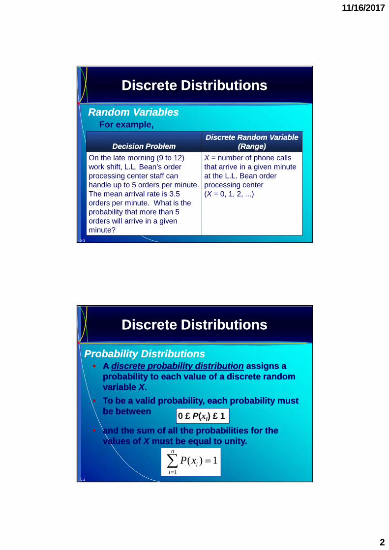
(Range)(Range)On the late morning (9 to 12)work shift, L.L. Bean’s orderprocessing center staff canhandle up to 5 orders per minute.The mean arrival rate is 3.5orders per minute. What is theprobability that more than 5orders will arrive in a givenminute?
X = number of phone callsthat arrive in a given minuteat the L.L. Bean orderprocessing center(X = 0, 1, 2, ...)
For example,
Discrete DistributionsDiscrete Distributions
Random VariablesRandom Variables
6-4
Probability DistributionsProbability Distributions•• AA discrete probability distributiondiscrete probability distribution assigns aassigns a
probability to each value of a discrete randomprobability to each value of a discrete randomvariablevariable XX..
•• To be a valid probability, each probability mustTo be a valid probability, each probability mustbe betweenbe between 0 P(xi) 1
•• and the sum of all the probabilities for theand the sum of all the probabilities for thevalues ofvalues of XX must be equal to unity.must be equal to unity.
1
( ) 1n
ii
P x
Discrete DistributionsDiscrete Distributions
11/16/2017
3
6-5
When you flip acoin three times,the sample spacehas eight equallylikely simple events.They are:
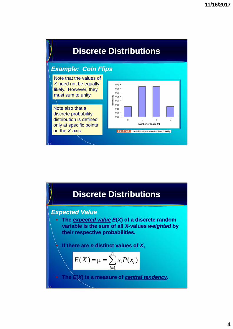
IfIf XX is the number of heads, thenis the number of heads, then XX is a random variableis a random variablewhose probability distribution is as follows:whose probability distribution is as follows:
Possible EventsPossible Events xx PP((xx))TTT 00 1/81/8HTT, THT, TTH 11 3/83/8HHT, HTH, THH 22 3/83/8HHH 33 1/81/8
Note that the values ofX need not be equallylikely. However, theymust sum to unity.
Note also that adiscrete probabilitydistribution is definedonly at specific pointson the X-axis.
Discrete DistributionsDiscrete Distributions
Example: Coin FlipsExample: Coin Flips
6-8
•• TheThe expected valueexpected value EE((XX) of a discrete random) of a discrete randomvariable is the sum of allvariable is the sum of all XX--valuesvalues weightedweighted bybytheir respective probabilities.their respective probabilities.
•• TheThe EE((XX) is a measure of) is a measure of central tendencycentral tendency..
•• If there areIf there are nn distinct values ofdistinct values of XX,,
1
( ) ( )n
i ii
E X x P x
Discrete DistributionsDiscrete Distributions
Expected ValueExpected Value
11/16/2017
5
6-9
The probability distribution of emergency serviceThe probability distribution of emergency servicecalls on Sunday by Ace Appliance Repair is:calls on Sunday by Ace Appliance Repair is:
What is the average or expectednumber of service calls?
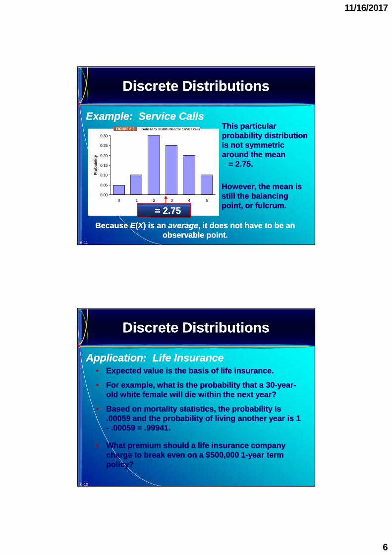
xx PP((xx))0 0.051 0.102 0.303 0.254 0.205 0.10
Total 1.00
Discrete DistributionsDiscrete Distributions
Example: Service CallsExample: Service Calls
6-10
The sum of theThe sum of the xPxP((xx))column is the expectedcolumn is the expectedvalue or mean of thevalue or mean of thediscrete distribution.discrete distribution.
This particularThis particularprobability distributionprobability distributionis not symmetricis not symmetricaround the meanaround the meanmm== 22..7575..
However, the mean isHowever, the mean isstill the balancingstill the balancingpoint, or fulcrum.point, or fulcrum.mm== 22..7575
BecauseBecause EE((XX) is an) is an averageaverage, it does not have to be an, it does not have to be anobservable point.observable point.
Discrete DistributionsDiscrete Distributions
Example: Service CallsExample: Service Calls
6-12
•• Expected value is the basis of life insurance.Expected value is the basis of life insurance.
•• For example, what is the probability that aFor example, what is the probability that a 3030--yearyear--old white female will die within the next year?old white female will die within the next year?
•• Based on mortality statistics, the probability isBased on mortality statistics, the probability is..0005900059 and the probability of living another year isand the probability of living another year is 11-- ..0005900059 = .= .9994199941..
•• What premium should a life insurance companyWhat premium should a life insurance companycharge to break even on a $charge to break even on a $500500,,000 1000 1--year termyear termpolicy?policy?
Discrete DistributionsDiscrete Distributions
Application: Life InsuranceApplication: Life Insurance
11/16/2017
7
6-13
LetLet XX be the amount paid by the company to settle thebe the amount paid by the company to settle thepolicy.policy.
Event x P(x) xP(x)Live 0 .99941 0.00Die 500,000 .00059 295.00
Total 1.00000 295.00Source: Centers for Disease Control and Prevention,National Vital Statistics Reports, 47, no. 28 (1999).
The total expectedThe total expectedpayout ispayout is
So, the premium should be $So, the premium should be $295295 plus whatever returnplus whatever returnthe company needs to cover administrative overheadthe company needs to cover administrative overhead
and profit.and profit.
Discrete DistributionsDiscrete Distributions
Application: Life InsuranceApplication: Life Insurance
6-14
•• Expected value can be applied to raffles andExpected value can be applied to raffles andlotteries.lotteries.
•• If it costs $If it costs $22 to buy a ticket in a raffle to win ato buy a ticket in a raffle to win anew car worth $new car worth $5555,,000000 andand 2929,,346346 raffle ticketsraffle ticketsare sold, what is the expected value of a raffleare sold, what is the expected value of a raffleticket?ticket?
•• If you buyIf you buy 11 ticket, what is the chance you willticket, what is the chance you will
•• Now, calculate theNow, calculate the EE((XX):):
E(X) = (value if you win)P(win) + (value if you lose)P(lose)
= (55,000) 129,346
+ (0) 29,34529,346
= (55,000)(.000034076) + (0)(.999965924) = $1.87
•• The raffle ticket is actually worth $The raffle ticket is actually worth $11..8787. Is it. Is itworth spending $worth spending $22..0000 for it?for it?
•• AnAn actuarially fairactuarially fair insurance program mustinsurance program mustcollect as much in overall revenue as it payscollect as much in overall revenue as it paysout in claims.out in claims.
•• Accomplish this by setting the premiums toAccomplish this by setting the premiums toreflect empirical experience with the insuredreflect empirical experience with the insuredgroup.group.
•• If the pool of insured persons is large enough,If the pool of insured persons is large enough,the total payout is predictable.the total payout is predictable.
Discrete DistributionsDiscrete Distributions
Actuarial FairnessActuarial Fairness
11/16/2017
9
6-17
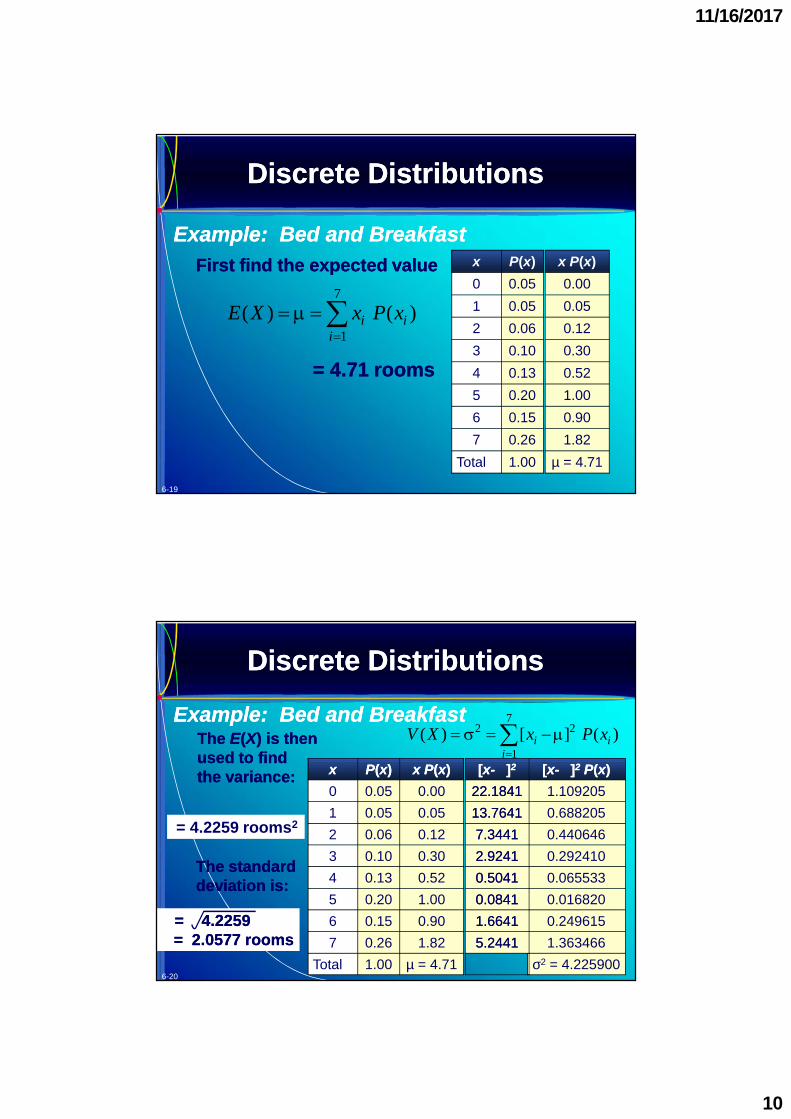
•• If there areIf there are nn distinct values ofdistinct values of XX, then the, then the variancevarianceof a discrete random variable is:of a discrete random variable is:
•• The variance is aThe variance is a weightedweighted average of theaverage of the dispersiondispersionabout the mean and is denoted either asabout the mean and is denoted either asss22 oror VV((XX).).
2 2
1
( ) [ ] ( )n
i ii
V X x P x
•• TheThe standard deviationstandard deviation is the square root of theis the square root of thevariance and is denotedvariance and is denotedss..
2 ( )V X
Discrete DistributionsDiscrete Distributions
Variance and Standard DeviationVariance and Standard Deviation
6-18
The probabilitydistribution ofroom rentals
during February is:
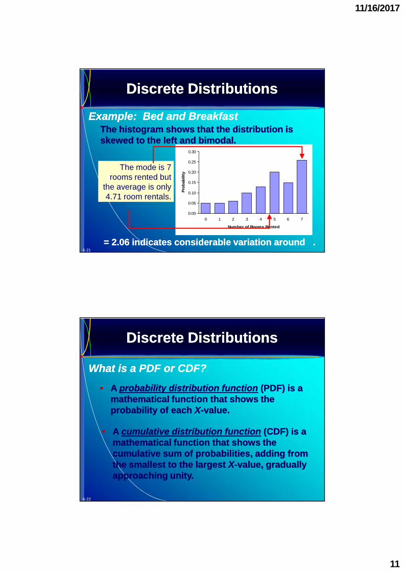
The Bay Street Inn is aThe Bay Street Inn is a 77--room bedroom bed--andand--breakfast inbreakfast inSanta Theresa, Ca.Santa Theresa, Ca.
x P(x)0 0.051 0.052 0.063 0.104 0.135 0.206 0.157 0.26
Total 1.00
Discrete DistributionsDiscrete Distributions
Example: Bed and BreakfastExample: Bed and Breakfast
11/16/2017
10
6-19
First find the expected valueFirst find the expected value x P(x)0 0.051 0.052 0.063 0.104 0.135 0.206 0.157 0.26
Total 1.00
7
1
( ) ( )i ii
E X x P x
= 4.71 rooms= 4.71 rooms
x P(x)0.000.050.120.300.521.000.901.82
µ = 4.71
Discrete DistributionsDiscrete Distributions
Example: Bed and BreakfastExample: Bed and Breakfast
6-20
TheThe EE((XX) is then) is thenused to findused to findthe variance:the variance: xx PP((xx)) x Px P((xx))
Example: Bed and BreakfastExample: Bed and Breakfast
6-22
•• AA probability distribution functionprobability distribution function (PDF) is a(PDF) is amathematical function that shows themathematical function that shows theprobability of eachprobability of each XX--value.value.
•• AA cumulative distribution functioncumulative distribution function (CDF) is a(CDF) is amathematical function that shows themathematical function that shows thecumulative sum of probabilities, adding fromcumulative sum of probabilities, adding fromthe smallest to the largestthe smallest to the largest XX--value, graduallyvalue, graduallyapproaching unity.approaching unity.
Discrete DistributionsDiscrete Distributions
What is a PDF or CDF?What is a PDF or CDF?
11/16/2017
12
6-23
0.00
0.05
0.10
0.15
0.20
0.25
0 1 2 3 4 5 6 7 8 9 10 11 12 13 14
Value of X
Prob
abili
ty
0.000.100.200.300.400.50
0.600.700.800.901.00
0 1 2 3 4 5 6 7 8 9 10 11 12 13 14
Value of X
Prob
abili
ty
Illustrative PDFIllustrative PDF(Probability Density Function)(Probability Density Function)
Cumulative CDFCumulative CDF(Cumulative Density Function)(Cumulative Density Function)
Consider the following illustrative histograms:Consider the following illustrative histograms:
The equations for these functions depend on theThe equations for these functions depend on theparameter(s)parameter(s) of the distribution.of the distribution.
Discrete DistributionsDiscrete Distributions
What is a PDF or CDF?What is a PDF or CDF?
6-24
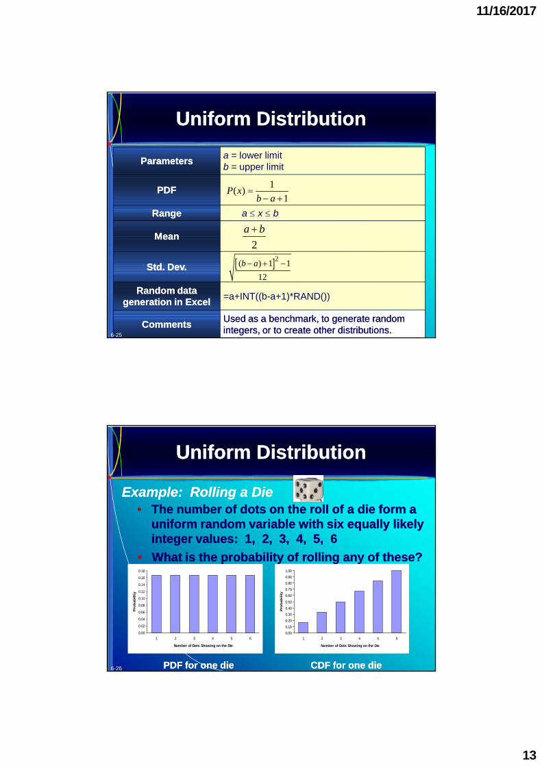
Characteristics of the Uniform DistributionCharacteristics of the Uniform Distribution•• TheThe uniform distributionuniform distribution describes a randomdescribes a random
variable with a finite number of integer valuesvariable with a finite number of integer valuesfromfrom aa toto bb (the only two parameters).(the only two parameters).
•• Each value of the random variable is equallyEach value of the random variable is equallylikely to occur.likely to occur.
•• Consider the following summary of theConsider the following summary of theuniform distribution:uniform distribution:
Uniform DistributionUniform Distribution
11/16/2017
13
ParametersParameters a = lower limitb = upper limit
PDFPDF
RangeRange a x b
MeanMean
Std. Dev.Std. Dev.
Random dataRandom datageneration in Excelgeneration in Excel =a+INT((b-a+1)*RAND())
CommentsComments Used as a benchmark, to generate randomUsed as a benchmark, to generate randomintegers, or to create other distributions.integers, or to create other distributions.
2( ) 1 1
12
b a
1( )
1P x
b a
2
a b
Uniform DistributionUniform Distribution
6-25
6-26
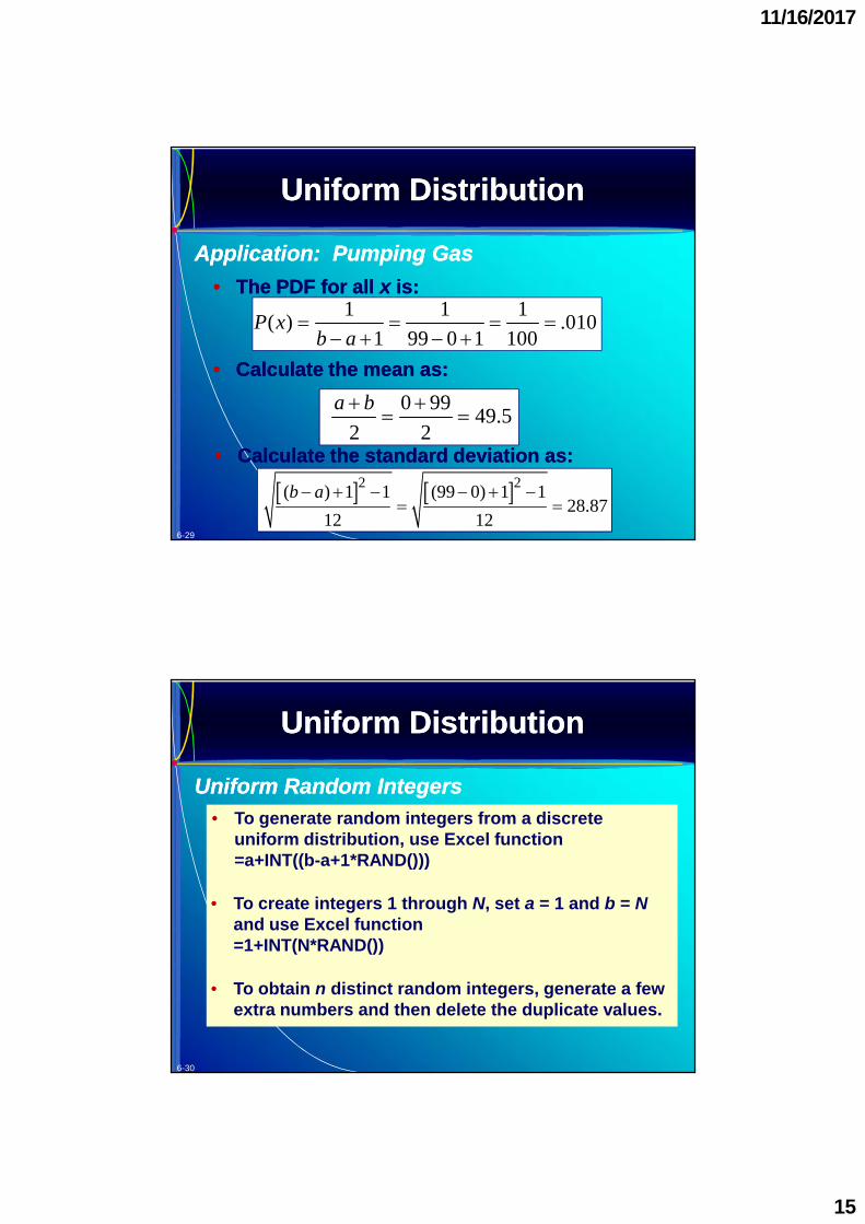
•• The number of dots on the roll of a die form aThe number of dots on the roll of a die form auniform random variable with six equally likelyuniform random variable with six equally likelyinteger values:integer values: 11,, 22,, 33,, 44,, 55,, 66
0.00
0.02
0.04
0.06
0.08
0.10
0.12
0.14
0.16
0.18
1 2 3 4 5 6
Number of Dots Showing on the Die
Pro
bab
ility
0.000.100.200.300.400.50
0.600.700.800.901.00
1 2 3 4 5 6
Number of Dots Showing on the Die
Pro
bab
ility
PDF for one diePDF for one die CDF for one dieCDF for one die
•• What is the probability of rolling any of these?What is the probability of rolling any of these?
Uniform DistributionUniform Distribution
Example: Rolling a DieExample: Rolling a Die
11/16/2017
14
6-27
•• The PDF for allThe PDF for all xx is:is:
•• Calculate the standard deviation as:Calculate the standard deviation as:
•• Calculate the mean as:Calculate the mean as:
1 1 1( )
1 6 1 1 6P x
b a
1 63.5
2 2
a b
2 2( ) 1 1 (6 1) 1 1
1.70812 12
b a
Uniform DistributionUniform Distribution
Example: Rolling a DieExample: Rolling a Die
6-28
On a gas pump, the last two digits (pennies)On a gas pump, the last two digits (pennies)displayed will be a uniform random integerdisplayed will be a uniform random integer(assuming the pump stops automatically).(assuming the pump stops automatically).
Application: Pumping GasApplication: Pumping Gas (Figure 6.9)
11/16/2017
15
6-29
•• The PDF for allThe PDF for all xx is:is:
•• Calculate the standard deviation as:Calculate the standard deviation as:
•• Calculate the mean as:Calculate the mean as:
1 1 1( ) .010
1 99 0 1 100P x
b a
0 9949.5
2 2
a b
2 2( ) 1 1 (99 0) 1 1
28.8712 12
b a
Uniform DistributionUniform Distribution
Application: Pumping GasApplication: Pumping Gas
6-30
• To generate random integers from a discreteuniform distribution, use Excel function=a+INT((b-a+1*RAND()))
• To obtain n distinct random integers, generate a fewextra numbers and then delete the duplicate values.
• To create integers 1 through N, set a = 1 and b = Nand use Excel function=1+INT(N*RAND())
Uniform DistributionUniform Distribution
Uniform Random IntegersUniform Random Integers
11/16/2017
16
6-31
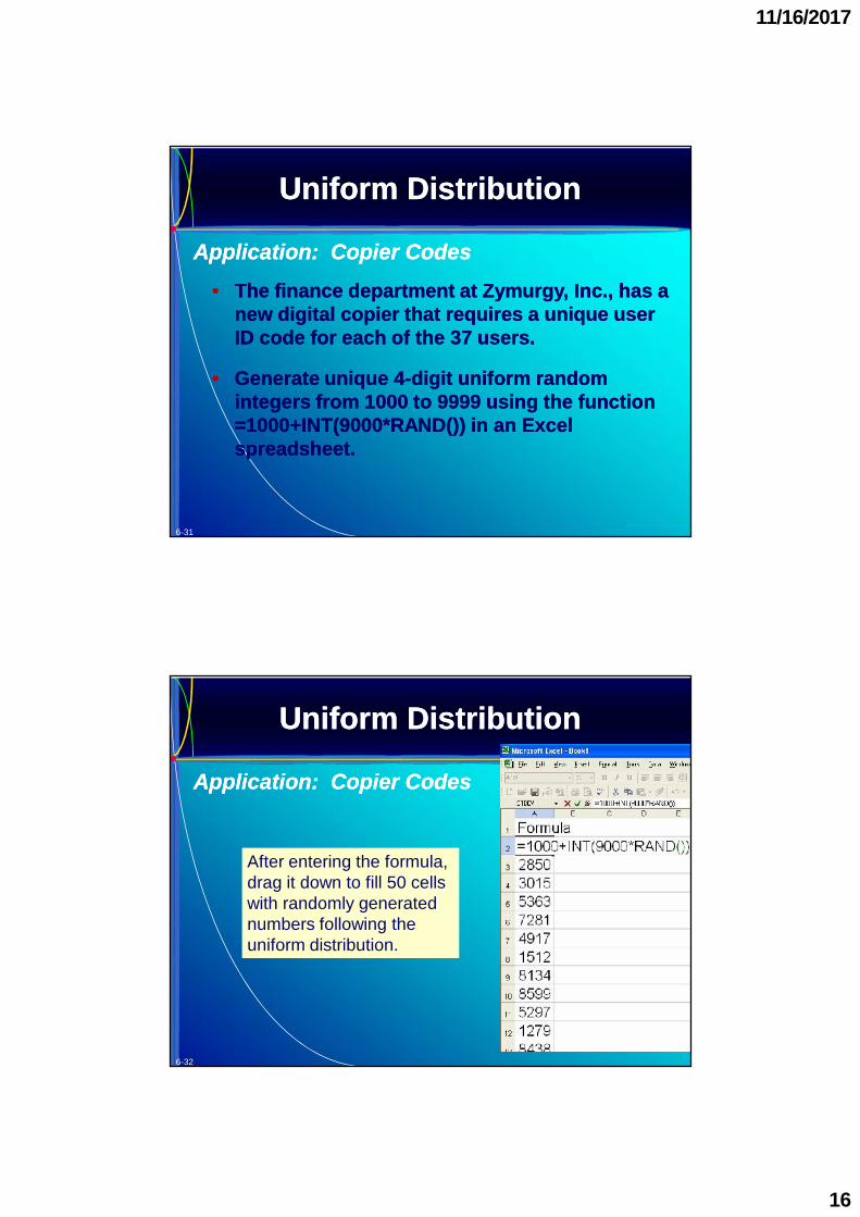
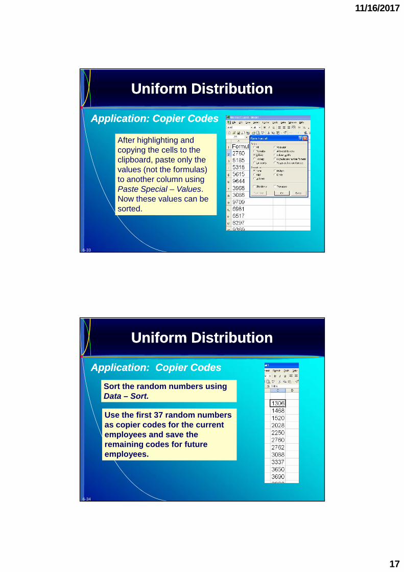
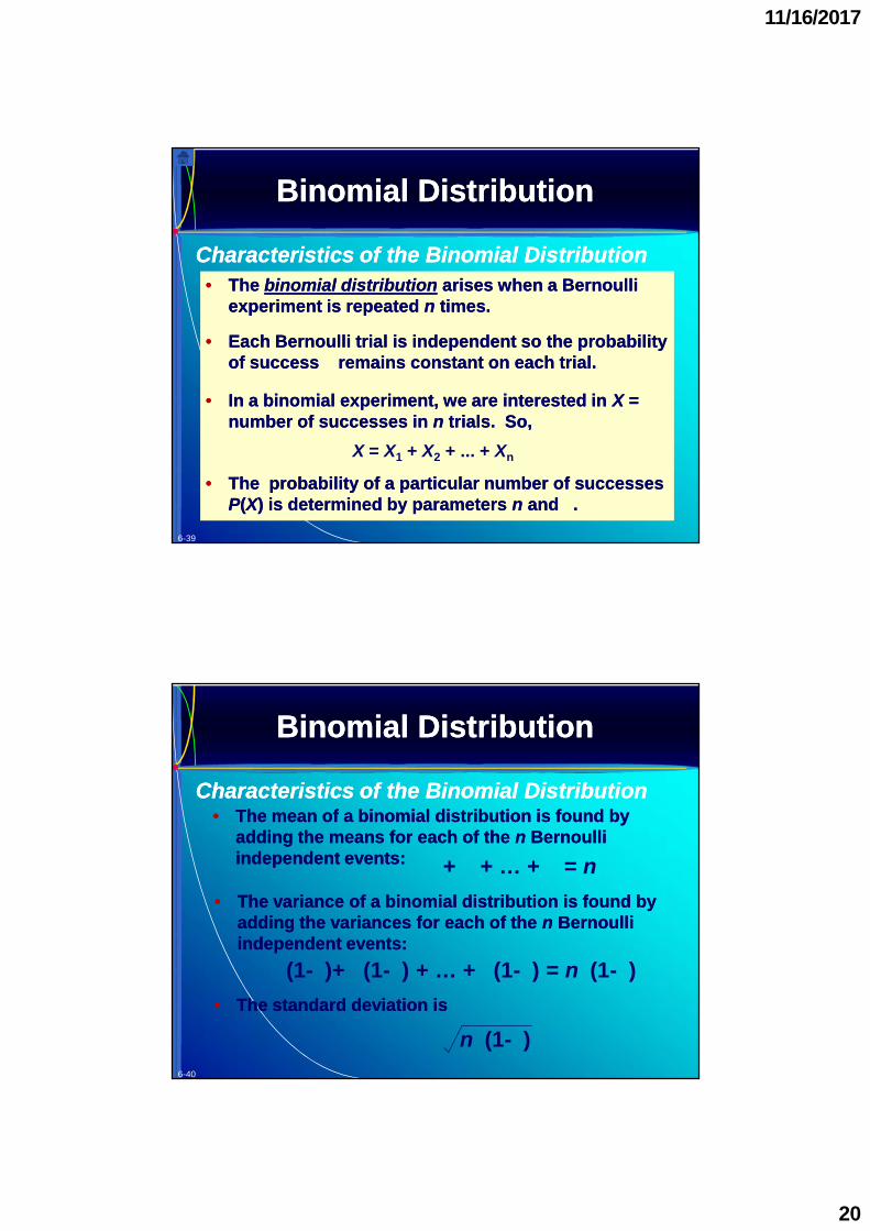
•• The finance department at Zymurgy, Inc., has aThe finance department at Zymurgy, Inc., has anew digital copier that requires a unique usernew digital copier that requires a unique userID code for each of theID code for each of the 3737 users.users.
•• Generate uniqueGenerate unique 44--digit uniform randomdigit uniform randomintegers fromintegers from 10001000 toto 99999999 using the functionusing the function==10001000+INT(+INT(90009000*RAND()) in an Excel*RAND()) in an Excelspreadsheet.spreadsheet.
After highlighting andcopying the cells to theclipboard, paste only thevalues (not the formulas)to another column usingPaste Special – Values.Now these values can besorted.
Here is theuniformdistribution for onedie fromLearningStats.
Uniform DistributionUniform Distribution
Uniform Model inUniform Model in LearningStatsLearningStats
6-36
•• A random experiment with onlyA random experiment with only 22 outcomes is aoutcomes is aBernoulli experimentBernoulli experiment..
•• One outcome is arbitrarily labeled aOne outcome is arbitrarily labeled a“success” (denoted“success” (denoted XX == 11) and the other a “failure”) and the other a “failure”(denoted(denoted XX == 00).).
•• “Success” is usually defined as the less likely“Success” is usually defined as the less likelyoutcome so thatoutcome so thatpp< .< .55 for convenience.for convenience.
Bernoulli ExperimentsBernoulli Experiments
Bernoulli DistributionBernoulli Distribution
11/16/2017
19
Bernoulli Experiment Possible Outcomes Probability of“Success”
Flip a coinFlip a coin 1 = heads0 = tails
π = .50
Consider the following Bernoulli experiments:Consider the following Bernoulli experiments:
Inspect a jet turbineInspect a jet turbinebladeblade
1 = crack found0 = no crack found
π = .001
Purchase a tank of gasPurchase a tank of gas 1 = pay by credit card0 = do not pay by credit
card
π = .78
Do a mammogram testDo a mammogram test 1 = positive test0 = negative test
π = .0004
Bernoulli ExperimentsBernoulli Experiments
Bernoulli DistributionBernoulli Distribution
6-37
6-38
2
2 2 2
1
( ) ( ) ( ) (0 ) (1 ) (1 ) ( ) (1 )i ii
V X x E X P x
•• The expected value (mean) of a Bernoulli experimentThe expected value (mean) of a Bernoulli experimentis calculated as:is calculated as:
2
1
( ) ( ) (0)(1 ) (1)( )i ii
E X x P x
•• The variance of a Bernoulli experiment is calculatedThe variance of a Bernoulli experiment is calculated
as:as:
•• The mean and variance are useful in developing theThe mean and variance are useful in developing thenext model.next model.
Bernoulli DistributionBernoulli Distribution
Bernoulli ExperimentsBernoulli Experiments
11/16/2017
20
6-39
•• TheThe binomial distributionbinomial distribution arises when a Bernoulliarises when a Bernoulliexperiment is repeatedexperiment is repeated nn times.times.
•• Each Bernoulli trial is independent so the probabilityEach Bernoulli trial is independent so the probabilityof successof successppremains constant on each trial.remains constant on each trial.
•• In a binomial experiment, we are interested inIn a binomial experiment, we are interested in XX ==number of successes innumber of successes in nn trials. So,trials. So,
X = X1 + X2 + ... + Xn
•• The probability of a particular number of successesThe probability of a particular number of successesPP((XX) is determined by parameters) is determined by parameters nn andandpp..
Binomial DistributionBinomial Distribution
Characteristics of the Binomial DistributionCharacteristics of the Binomial Distribution
6-40
•• The mean of a binomial distribution is found byThe mean of a binomial distribution is found byadding the means for each of theadding the means for each of the nn BernoulliBernoulliindependent events:independent events: p+p+ … +p= np
•• The variance of a binomial distribution is found byThe variance of a binomial distribution is found byadding the variances for each of theadding the variances for each of the nn BernoulliBernoulliindependent events:independent events:p(1-p)+ p(1-p) + … +p(1-p) = np(1-p)
•• The standard deviation isThe standard deviation is
np(1-p)
Binomial DistributionBinomial Distribution
Characteristics of the Binomial DistributionCharacteristics of the Binomial Distribution
11/16/2017
21
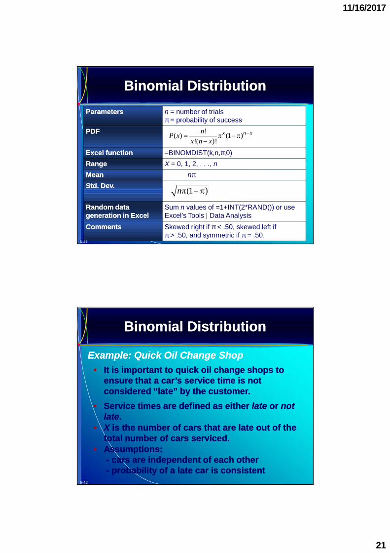
ParametersParameters n = number of trialsπ = probability of success
PDFPDF
Excel functionExcel function =BINOMDIST(k,n,π,0)RangeRange X = 0, 1, 2, . . ., nMeanMean nπStd. Dev.Std. Dev.
Random dataRandom datageneration in Excelgeneration in Excel
Sum n values of =1+INT(2*RAND()) or useExcel’s Tools | Data Analysis
CommentsComments Skewed right if π < .50, skewed left ifπ > .50, and symmetric if π = .50.
!( ) (1 )
!( )!x n xn
P xx n x
(1 )n
Binomial DistributionBinomial Distribution
6-41
6-42
•• It is important to quick oil change shops toIt is important to quick oil change shops toensure that a car’s service time is notensure that a car’s service time is notconsidered “late” by the customer.considered “late” by the customer.
•• Service times are defined as eitherService times are defined as either latelate oror notnotlatelate..
•• XX is the number of cars that are late out of theis the number of cars that are late out of thetotal number of cars serviced.total number of cars serviced.
•• Assumptions:Assumptions:-- cars are independent of each othercars are independent of each other-- probability of a late car is consistentprobability of a late car is consistent
•• What is the probability that exactly 2 of theWhat is the probability that exactly 2 of thenextnext nn = 10 cars serviced are late (= 10 cars serviced are late (PP((XX = 2))?= 2))?
•• PP(car is late) =(car is late) =pp= .= .1010
•• PP(car not late) = 1(car not late) = 1 --pp= .90= .90!
•• Alternatively, we could findAlternatively, we could find PP((XX == 22) using the Excel) using the Excelfunction =BINOMDIST(k,n,function =BINOMDIST(k,n,pp,,00) where) where
k = the number of “successes” in n trialsn = the number of independent trialsp= probability of
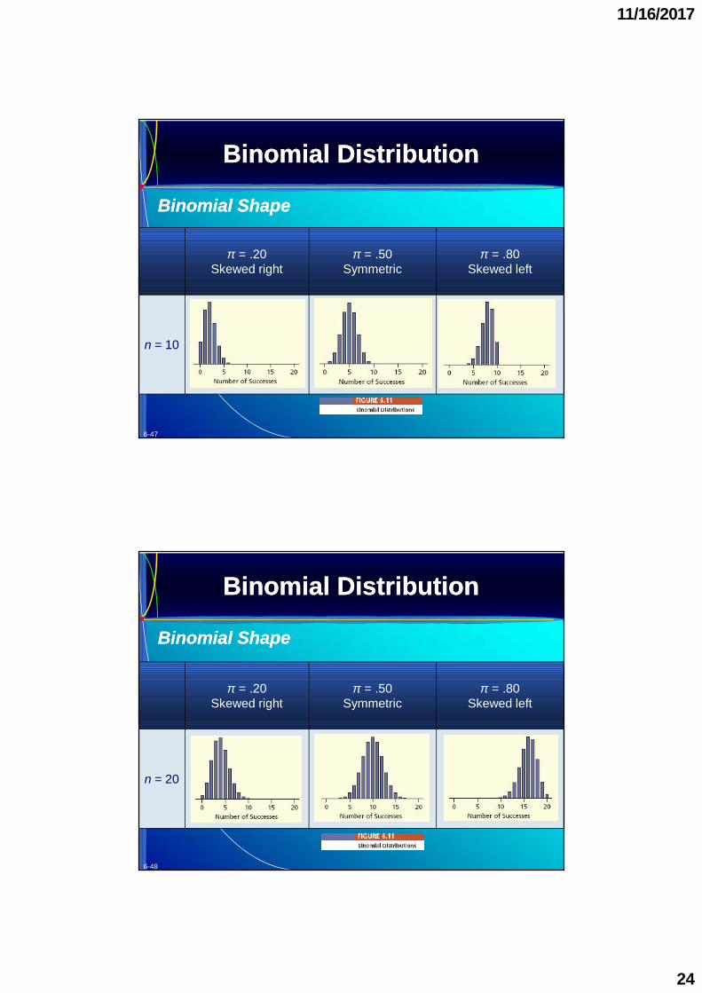
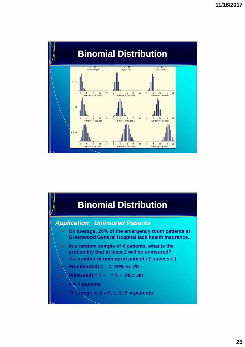
•• A binomial distribution isA binomial distribution isskewed right ifskewed right ifpp< .50,< .50,skewed left ifskewed left ifpp> .50,> .50,and symmetric ifand symmetric ifpp= .50= .50
•• SkewnessSkewness decreases asdecreases as nn increases,increases,regardless of the value ofregardless of the value ofpp..
•• To illustrate, consider the following graphs:To illustrate, consider the following graphs:
Binomial DistributionBinomial Distribution
Binomial ShapeBinomial Shape
6-46
π = .20Skewed right
π = .50Symmetric
π = .80Skewed left
n = 5
Binomial DistributionBinomial Distribution
Binomial ShapeBinomial Shape
11/16/2017
24
6-47
π = .20Skewed right
π = .50Symmetric
π = .80Skewed left
n = 10
Binomial DistributionBinomial Distribution
Binomial ShapeBinomial Shape
6-48
π = .20Skewed right
π = .50Symmetric
π = .80Skewed left
n = 20
Binomial DistributionBinomial Distribution
Binomial ShapeBinomial Shape
11/16/2017
25
Binomial DistributionBinomial Distribution
6-49
6-50
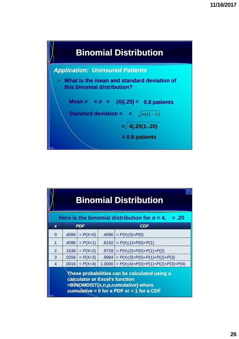
• On average, 20% of the emergency room patients atGreenwood General Hospital lack health insurance.
• In a random sample of 4 patients, what is theprobability that at least 2 will be uninsured?
• X = number of uninsured patients (“success”)•• PP(uninsured) =(uninsured) =pp== 2020% or .% or .2020
These probabilities can be calculated using aThese probabilities can be calculated using acalculator or Excel’s functioncalculator or Excel’s function=BINOMDIST(=BINOMDIST(x,n,p,cumulativex,n,p,cumulative) where) wherecumulativecumulative = 0 for a PDF or = 1 for a CDF= 0 for a PDF or = 1 for a CDF
Binomial probabilities can also be determined byBinomial probabilities can also be determined bylooking them up in a table (looking them up in a table (Appendix AAppendix A) for) forselected values ofselected values of nn (row) and(row) andpp(column).(column).
n X 0.01 0.02 0.05 0.10 0.15 0.20 0.30 0.40 0.50 0.60 0.70 0.80 0.85 0.90 0.95 0.98 0.99
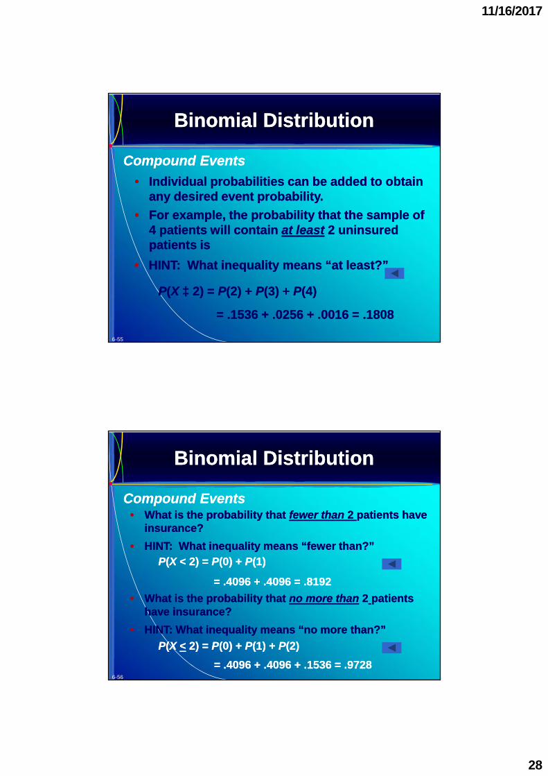
•• Individual probabilities can be added to obtainIndividual probabilities can be added to obtainany desired event probability.any desired event probability.
•• For example, the probability that the sample ofFor example, the probability that the sample of44 patients will containpatients will contain at leastat least 22 uninsureduninsuredpatients ispatients is
•• Use Excel’s Insert | Function menu to calculateUse Excel’s Insert | Function menu to calculatethe probability ofthe probability of xx == 6767 successes insuccesses in nn == 11,,024024trials with probabilitytrials with probabilitypp= .= .048048..
•• Or use =BINOMDIST(Or use =BINOMDIST(6767,,10241024,,00..048048,,00))
Binomial DistributionBinomial Distribution
Using Software: ExcelUsing Software: Excel
11/16/2017
30
6-59
•• Compute an entire binomial PDF for anyCompute an entire binomial PDF for any nn andandpp(e.g.,(e.g., nn== 1010,,pp= .= .5050) in) in MegaStatMegaStat..
Binomial DistributionBinomial Distribution
Using Software:Using Software: MegaStatMegaStat
6-60
MegaStatMegaStat also gives you the option to create aalso gives you the option to create agraph of the PDF:graph of the PDF:
5.000 expected value2.500 variance1.581 standard deviation
Binomial distribution (n = 10, p = 0.5)
0.00
0.05
0.10
0.15
0.20
0.25
0.30
0 1 2 3 4 5 6 7 8 9 10
X
p(X
)
Binomial DistributionBinomial Distribution
Using Software:Using Software: MegaStatMegaStat
11/16/2017
31
6-61
•• UsingUsing Visual StatisticsVisual Statistics ModuleModule 44, here is a binomial, here is a binomialdistribution fordistribution for nn == 1010 andandpp= .= .5050::
Copy and paste graphas a bitmap.Copy and pasteprobabilities intoExcel.
“Spin” n and π and super-impose a normal curve onthe binomial distribution.
Binomial DistributionBinomial Distribution
Using Software: Visual StatisticsUsing Software: Visual Statistics
6-62
Here,Here, nn == 5050 andandpp= .= .095095..
Spin buttonslet you vary nand π.
Binomial DistributionBinomial Distribution
Using Software:Using Software: LearningStatsLearningStats
11/16/2017
32
6-63
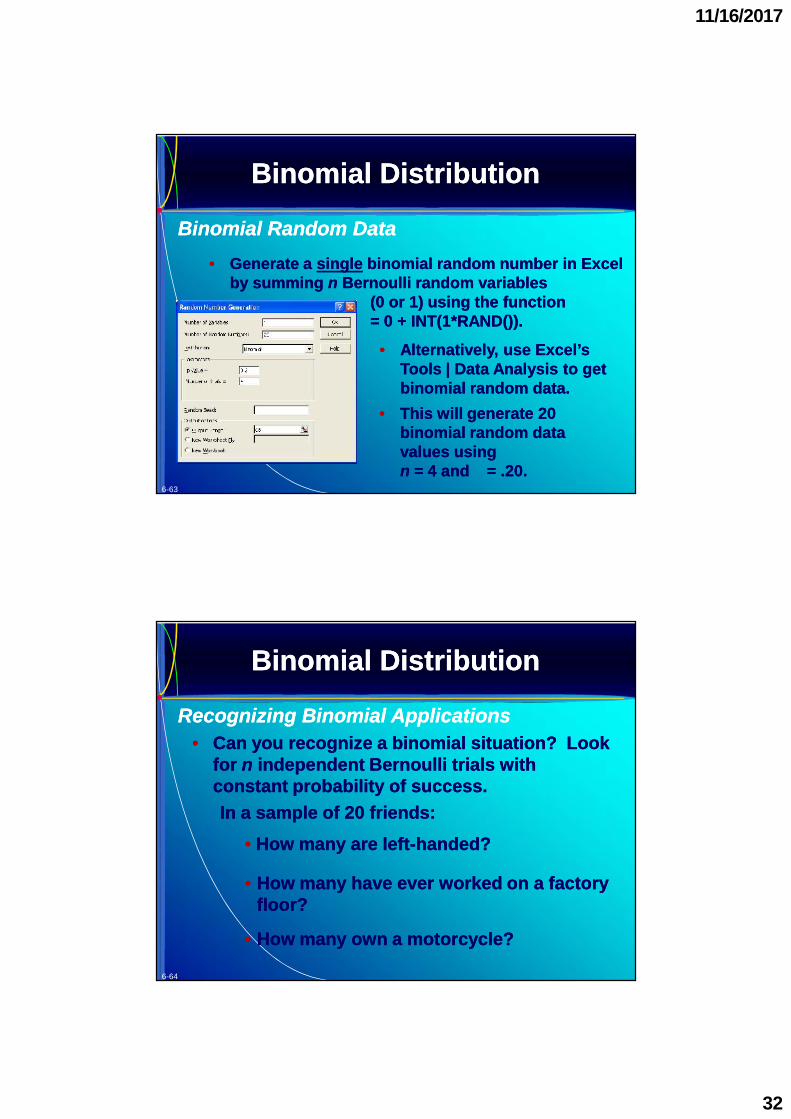
•• Generate aGenerate a singlesingle binomial random number in Excelbinomial random number in Excelby summingby summing nn Bernoulli random variablesBernoulli random variables
((00 oror 11) using the function) using the function== 00 + INT(+ INT(11*RAND()).*RAND()).
•• Alternatively, use Excel’sAlternatively, use Excel’sTools | Data Analysis to getTools | Data Analysis to getbinomial random data.binomial random data.
•• This will generateThis will generate 2020binomial random databinomial random datavalues usingvalues usingnn == 44 andandpp= .= .2020..
Binomial DistributionBinomial Distribution
Binomial Random DataBinomial Random Data
6-64
•• Can you recognize a binomial situation? LookCan you recognize a binomial situation? Lookforfor nn independent Bernoulli trials withindependent Bernoulli trials withconstant probability of success.constant probability of success.In a sample ofIn a sample of 2020 friends:friends:
•• How many are leftHow many are left--handed?handed?
•• How many have ever worked on a factoryHow many have ever worked on a factoryfloor?floor?
•• How many own a motorcycle?How many own a motorcycle?
•• Can you recognize a binomial situation?Can you recognize a binomial situation?In a sample ofIn a sample of 5050 cars in a parking lot:cars in a parking lot:
•• How many are parked endHow many are parked end--first?first?•• How many are blue?How many are blue?•• How many have hybrid engines?How many have hybrid engines?
In a sample ofIn a sample of 1010 emergency patients withemergency patients withchest pain:chest pain:
•• How many will be admitted?How many will be admitted?•• How many will need bypass surgery?How many will need bypass surgery?•• How many will be uninsured?How many will be uninsured?
•• TheThe Poisson distributionPoisson distribution was named forwas named forFrench mathematicianFrench mathematician SimSiméonéon Poisson (Poisson (17811781--18401840).).
•• The Poisson distribution describes theThe Poisson distribution describes thenumber of occurrences within a randomlynumber of occurrences within a randomlychosen unit of time or space.chosen unit of time or space.
•• For example, within a minute, hour,For example, within a minute, hour,day, square foot, or linear mile.day, square foot, or linear mile.
Poisson DistributionPoisson Distribution
Poisson ProcessesPoisson Processes
11/16/2017
34
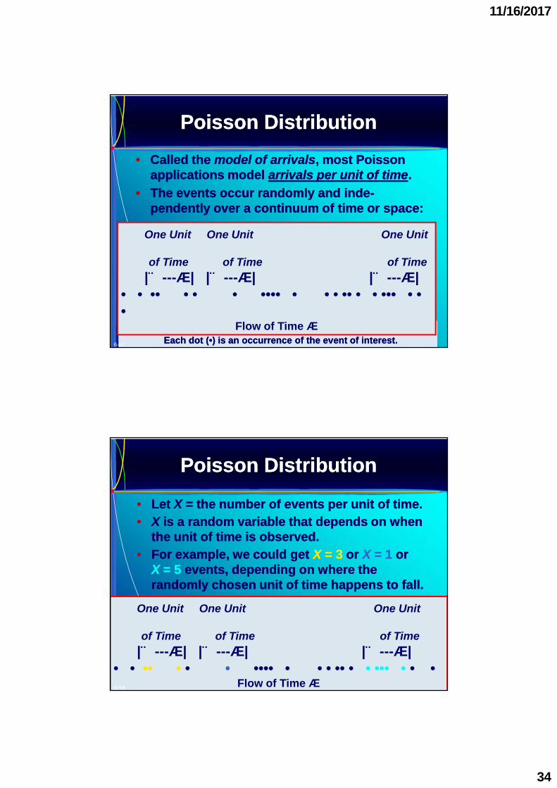
•• The events occur randomly andThe events occur randomly and indeinde--pendentlypendently over a continuum of time or space:over a continuum of time or space:
One Unit One Unit One Unit
of Time of Time of Time|---| |---| |---|
• • •• • • • •••• • • • •• • • ••• • ••
Flow of Time
•• Called theCalled the model of arrivalsmodel of arrivals, most Poisson, most Poissonapplications modelapplications model arrivals per unit of timearrivals per unit of time..
Each dot (Each dot (••) is an occurrence of the event of interest.) is an occurrence of the event of interest.
Poisson DistributionPoisson Distribution
6-67
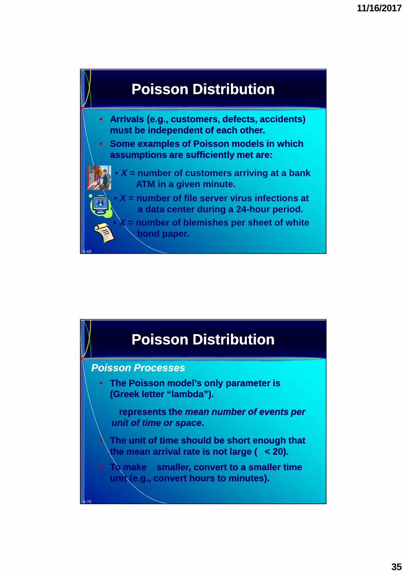
•• LetLet XX = the number of events per unit of time.= the number of events per unit of time.•• XX is a random variable that depends on whenis a random variable that depends on when
the unit of time is observed.the unit of time is observed.•• For example, we could getFor example, we could get XX == 33 oror XX == 11 oror
XX == 55 events, depending on where theevents, depending on where therandomly chosen unit of time happens to fall.randomly chosen unit of time happens to fall.
One Unit One Unit One Unit
of Time of Time of Time|---| |---| |---|
• • •• • • • •••• • • • •• • • ••• • • •Flow of Time
Poisson DistributionPoisson Distribution
6-68
11/16/2017
35
6-69
•• Arrivals (e.g., customers, defects, accidents)Arrivals (e.g., customers, defects, accidents)must be independent of each other.must be independent of each other.
•• Some examples of Poisson models in whichSome examples of Poisson models in whichassumptions are sufficiently met are:assumptions are sufficiently met are:
• X = number of customers arriving at a bankATM in a given minute.
• X = number of file server virus infections ata data center during a 24-hour period.
• X = number of blemishes per sheet of whitebond paper.
Poisson DistributionPoisson Distribution
6-70
llrepresents therepresents the mean number of events permean number of events perunit of time or spaceunit of time or space..
•• The unit of time should be short enough thatThe unit of time should be short enough thatthe mean arrival rate is not large (the mean arrival rate is not large (ll<< 2020).).
•• To makeTo makellsmaller, convert to a smaller timesmaller, convert to a smaller timeunit (e.g., convert hours to minutes).unit (e.g., convert hours to minutes).
•• The Poisson model’s only parameter isThe Poisson model’s only parameter isll(Greek letter “lambda”).(Greek letter “lambda”).
Poisson DistributionPoisson Distribution
Poisson ProcessesPoisson Processes
11/16/2017
36
6-71
•• The number of events that can occur in aThe number of events that can occur in agiven unit of time is not bounded, thereforegiven unit of time is not bounded, therefore XXhas no obvious limit.has no obvious limit.
•• However, Poisson probabilities taper offHowever, Poisson probabilities taper offtoward zero astoward zero as XX increases.increases.
•• The Poisson distribution is sometimes calledThe Poisson distribution is sometimes calledthethe model of rare eventsmodel of rare events..
Poisson DistributionPoisson Distribution
Poisson ProcessesPoisson Processes
6-72
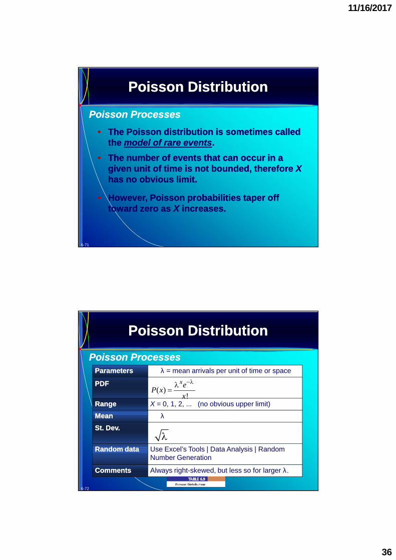
ParametersParameters λ = mean arrivals per unit of time or space
PDFPDF
RangeRange X = 0, 1, 2, ... (no obvious upper limit)
MeanMean λ
St. Dev.St. Dev.
Random dataRandom data Use Excel’s Tools | Data Analysis | RandomNumber Generation
CommentsComments Always right-skewed, but less so for larger λ.
Poisson distributions are always rightPoisson distributions are always right--skewedskewedbut become less skewed and more bellbut become less skewed and more bell--shapedshapedasasllincreases.increases.
Poisson DistributionPoisson Distribution
Poisson ProcessesPoisson Processes
11/16/2017
38
6-75
Example: Credit Union CustomersExample: Credit Union Customers
•• Find the PDF, mean and standard deviation:Find the PDF, mean and standard deviation:
PDF =1.7(1.7)
( )! !
x xe eP x
x x
Mean =l= 1.7 customers per minute.
Standard deviation =s == 11..77 = 1.304 cust/min
•• On Thursday morning betweenOn Thursday morning between 99 A.M. andA.M. and 1010 A.M.A.M.customers arrive and enter the queue at the Oxnardcustomers arrive and enter the queue at the OxnardUniversity Credit Union at a mean rate ofUniversity Credit Union at a mean rate of 11..77customers per minute.customers per minute.
Poisson DistributionPoisson Distribution
6-76
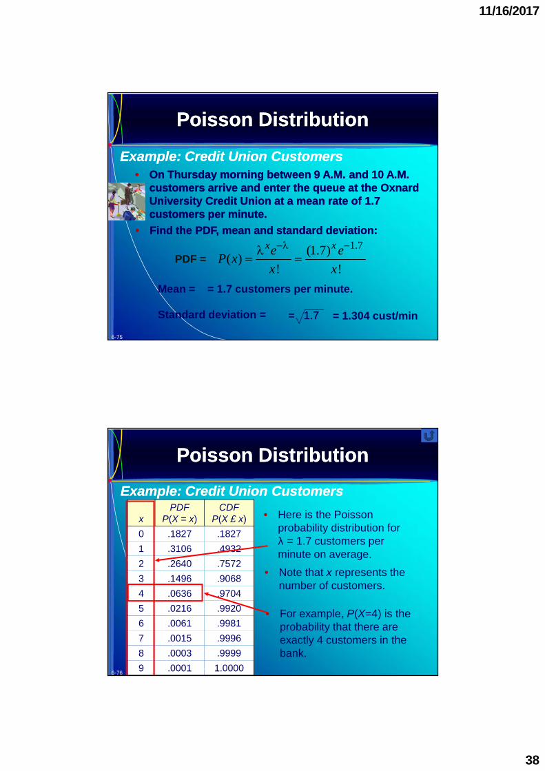
Example: Credit Union CustomersExample: Credit Union Customers• Here is the Poisson
probability distribution forλ = 1.7 customers perminute on average.
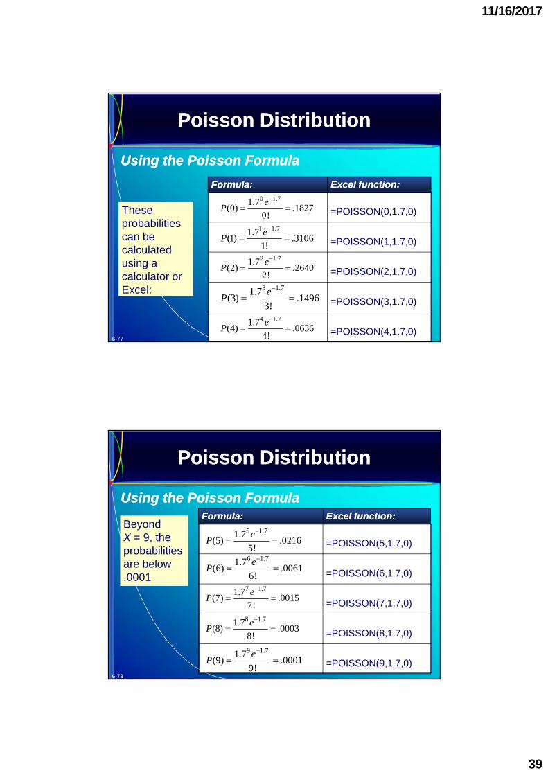
Using the Poisson FormulaUsing the Poisson Formula
6-78
Formula:Formula: Excel function:Excel function:
=POISSON(5,1.7,0)
=POISSON(6,1.7,0)
=POISSON(7,1.7,0)
=POISSON(8,1.7,0)
=POISSON(9,1.7,0)9 1.71.7
(9) .00019!
eP
8 1.71.7(8) .0003
8!
eP
7 1.71.7(7) .0015
7!
eP
6 1.71.7(6) .0061
6!
eP
5 1.71.7(5) .0216
5!
eP
BeyondX = 9, theprobabilitiesare below.0001
Poisson DistributionPoisson Distribution
Using the Poisson FormulaUsing the Poisson Formula
11/16/2017
40
6-79
•• Here are the graphs of the distributions:Here are the graphs of the distributions:
0.00
0.05
0.10
0.15
0.20
0.25
0.30
0.35
0 1 2 3 4 5 6 7 8 9
Number of Customer Arrivals
Prob
abili
ty
0.000.100.200.300.400.50
0.600.700.800.901.00
0 1 2 3 4 5 6 7 8 9
Number of Customer Arrivals
Prob
abili
ty
Poisson PDF forPoisson PDF forll== 11..77 Poisson CDF forPoisson CDF forll= 1.7= 1.7
•• The most likely event isThe most likely event is 11 arrival (arrival (PP((11)=.)=.31063106 oror3131..11% chance).% chance).
•• This will help the credit union schedule tellers.This will help the credit union schedule tellers.
Poisson DistributionPoisson Distribution
6-80
•• Cumulative probabilities can be evaluated byCumulative probabilities can be evaluated bysumming individualsumming individual XX probabilities.probabilities.
•• What is the probability that two or fewerWhat is the probability that two or fewercustomers will arrive in a given minute?customers will arrive in a given minute?
= .1827 + .3106 + .2640 = .7573
P(X < 2) = P(0) + P(1) + P(2)
Poisson DistributionPoisson Distribution
Compound EventsCompound Events
11/16/2017
41
6-81
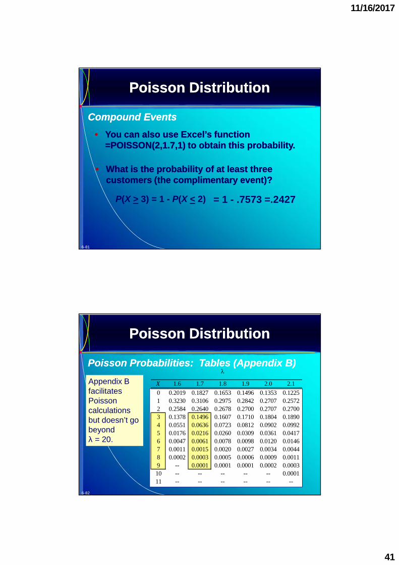
•• What is the probability of at least threeWhat is the probability of at least threecustomers (the complimentary event)?customers (the complimentary event)?
= 1 - .7573 =.2427P(X > 3) = 1 - P(X < 2)
•• You can also use Excel’s functionYou can also use Excel’s function=POISSON(2,1.7,1) to obtain this probability.=POISSON(2,1.7,1) to obtain this probability.
Poisson Probabilities: Tables (Appendix B)Poisson Probabilities: Tables (Appendix B)
11/16/2017
42
6-83
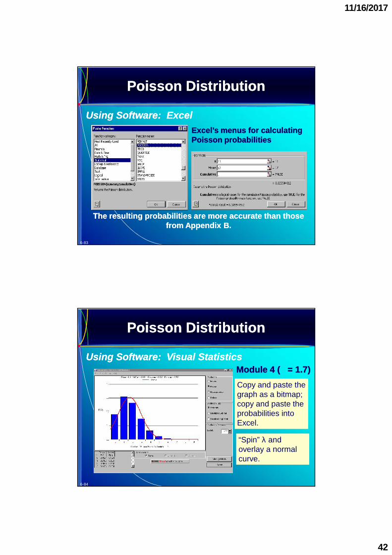
Excel’s menus for calculatingExcel’s menus for calculatingPoisson probabilitiesPoisson probabilities
The resulting probabilities are more accurate than thoseThe resulting probabilities are more accurate than thosefrom Appendix B.from Appendix B.
Poisson DistributionPoisson Distribution
Using Software: ExcelUsing Software: Excel
6-84
“Spin” λ andoverlay a normalcurve.
ModuleModule 44 ((ll== 11..77))Copy and paste thegraph as a bitmap;copy and paste theprobabilities intoExcel.
Poisson DistributionPoisson Distribution
Using Software: Visual StatisticsUsing Software: Visual Statistics
11/16/2017
43
6-85
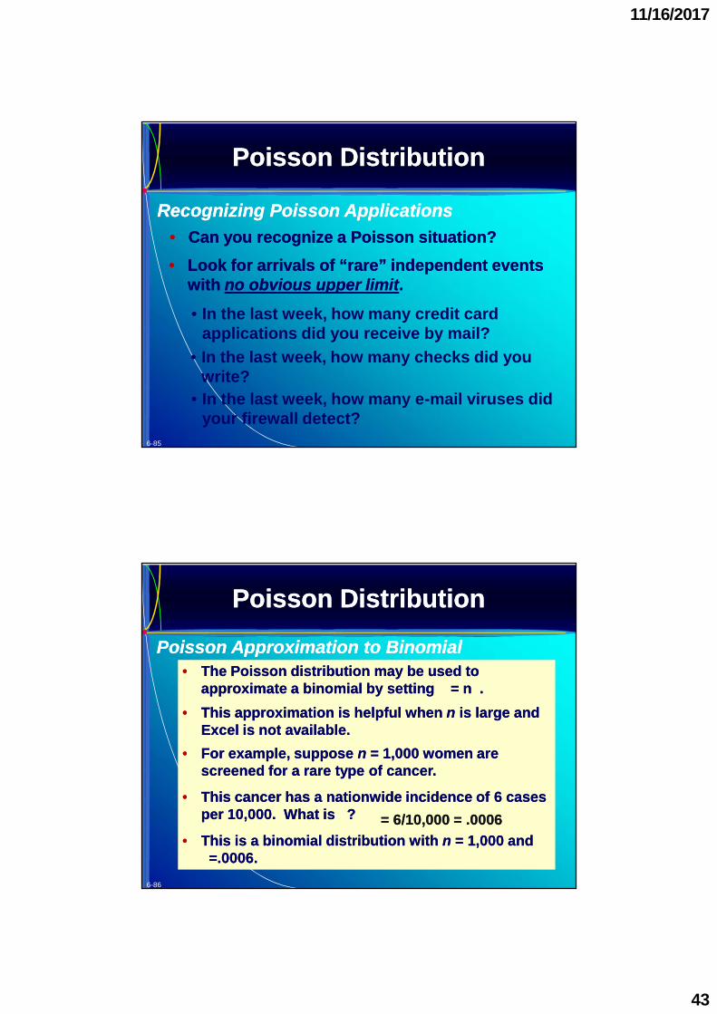
•• Can you recognize a Poisson situation?Can you recognize a Poisson situation?•• Look for arrivals of “rare” independent eventsLook for arrivals of “rare” independent events
withwith no obvious upper limitno obvious upper limit..
• In the last week, how many credit cardapplications did you receive by mail?
• In the last week, how many checks did youwrite?
• In the last week, how many e-mail viruses didyour firewall detect?
•• The Poisson distribution may be used toThe Poisson distribution may be used toapproximate a binomial by settingapproximate a binomial by settingll== nnpp..
•• This approximation is helpful whenThis approximation is helpful when nn is large andis large andExcel is not available.Excel is not available.
•• For example, supposeFor example, suppose nn == 11,,000000 women arewomen arescreened for a rare type of cancer.screened for a rare type of cancer.
•• This cancer has a nationwide incidence ofThis cancer has a nationwide incidence of 66 casescasesperper 1010,,000000. What is. What ispp?? pp== 66//1010,,000000 = .= .00060006
•• This is a binomial distribution withThis is a binomial distribution with nn == 11,,000000 andandpp=.=.00060006..
Poisson DistributionPoisson Distribution
Poisson Approximation to BinomialPoisson Approximation to Binomial
11/16/2017
44
6-87
•• SetSetll== nnpp
•• Since the binomial formula involves factorialsSince the binomial formula involves factorials(which are cumbersome as(which are cumbersome as nn increases), useincreases), usethe Poisson distribution as an approximation:the Poisson distribution as an approximation:
•• Now use Appendix B or the Poisson PDF toNow use Appendix B or the Poisson PDF tocalculate the probability ofcalculate the probability of xx successes. Forsuccesses. Forexample:example:
Poisson Approximation to BinomialPoisson Approximation to Binomial
6-88
Here is a comparison of Binomial probabilitiesHere is a comparison of Binomial probabilitiesand the respective Poisson approximations.and the respective Poisson approximations.
Poisson approximation:Poisson approximation: Actual Binomial probability:
P(0) = .60 e-0.6 / 0! = .5488 = .5487
P(1) = .61 e-0.6 / 1! = .3293 = .3294
P(2) = .62 e-0.6 / 2! = .0988 = .0988
2 1000 21000!(2) .0006 (1 .0006)
2!(1000 2)!P
1 1000 11000!(1) .0006 (1 .0006)
1!(1000 1)!P
0 1000 01000!(0) .0006 (1 .0006)
0!(1000 0)!P
Rule of thumb: the approximation is adequate ifRule of thumb: the approximation is adequate ifnn >> 20 and20 andpp<< .05..05.
Poisson DistributionPoisson Distribution
11/16/2017
45
6-89
•• TheThe hypergeometrichypergeometric distributiondistribution is similar tois similar tothe binomial distribution.the binomial distribution.
•• However, unlike the binomial, sampling isHowever, unlike the binomial, sampling iswithout replacementwithout replacement from a finite populationfrom a finite populationofof NN items.items.
•• TheThe hypergeometrichypergeometric distribution may bedistribution may beskewed right or left and is symmetric only ifskewed right or left and is symmetric only ifthe proportion of successes in the populationthe proportion of successes in the populationisis 5050%.%.
Characteristics of theCharacteristics of the HypergeometricHypergeometric Dist.Dist.
ParametersParameters N = number of items in the populationn = sample sizes = number of “successes” in population
PDFPDF
RangeRange X = max(0, n-N+s) x min(s, n)MeanMean nπ where π = s/N
St. Dev.St. Dev.
CommentsComments Similar to binomial, but sampling is without replacementfrom a finite population. Can be approximated by binomialwithπ = s/N if n/N < 0.05 (i.e., less than 5% sample).
Characteristics of theCharacteristics of the HypergeometricHypergeometric Dist.Dist.TheThe hypergeometrichypergeometric PDF uses the formula for combinations:PDF uses the formula for combinations:
nN
xnsNxs
C
CCxP )(
xs C
xnsN C
nN C6-91
6-92
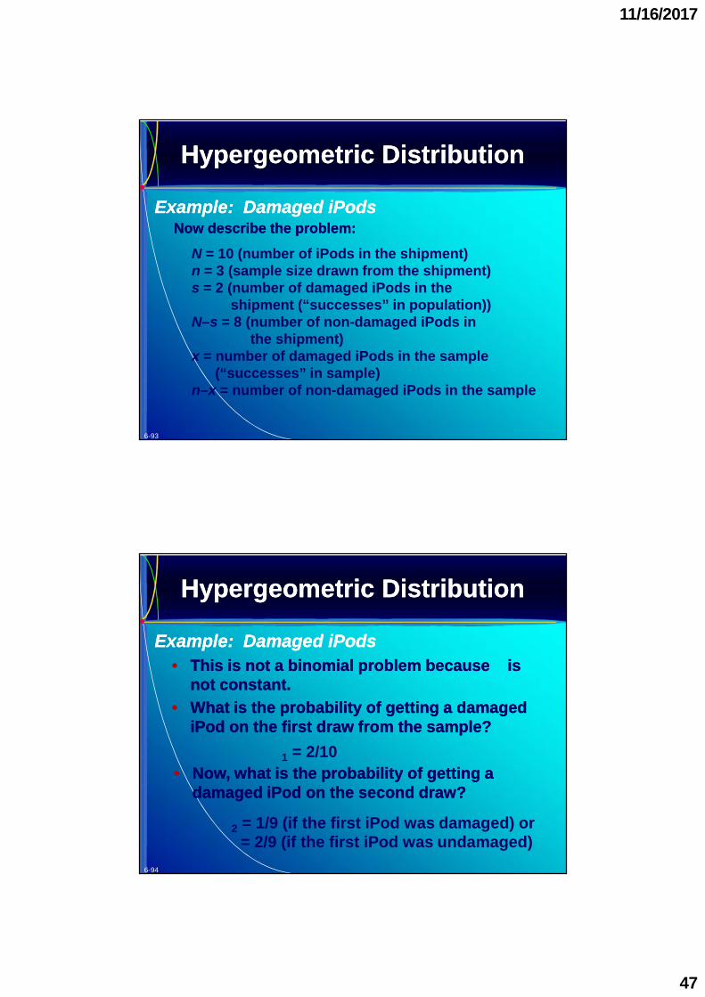
•• In a shipment ofIn a shipment of 1010 iPods,iPods, 22 were damagedwere damagedandand 88 are good.are good.
•• The receiving department at Best Buy tests aThe receiving department at Best Buy tests asample ofsample of 33 iPods at random to see if they areiPods at random to see if they aredefective.defective.
•• Let the random variableLet the random variable XX be the number ofbe the number ofdamaged iPods in the sample.damaged iPods in the sample.
•• This is not a binomial problem becauseThis is not a binomial problem becauseppisisnot constant.not constant.
•• What is the probability of getting a damagedWhat is the probability of getting a damagediPod on the first draw from the sample?iPod on the first draw from the sample?
p1 = 2/10•• Now, what is the probability of getting aNow, what is the probability of getting a
damaged iPod on the second draw?damaged iPod on the second draw?
p2 = 1/9 (if the first iPod was damaged) or= 2/9 (if the first iPod was undamaged)
Since there are onlySince there are only 22 damaged iPods in the population, thedamaged iPods in the population, theonly possible values ofonly possible values of xx areare 00,, 11, and, and 22. Here are the. Here are theprobabilities:probabilities:
= .= .46674667
= .= .46674667
= .= .06670667
=HYPGEOMDIST(0,3,2,10)
=HYPGEOMDIST(1,3,2,10)
=HYPGEOMDIST(2,3,2,10)
PDF FormulaPDF Formula Excel Function
HypergeometricHypergeometric DistributionDistributionUsing theUsing the HypergeometricHypergeometric FormulaFormula
11/16/2017
49
Since theSince the hypergeometrichypergeometric formula and tables areformula and tables aretedious and impractical, use Excel’stedious and impractical, use Excel’shypergeometrichypergeometric function to find probabilities.function to find probabilities.
ModuleModule 44, the probabilities are given below the graph., the probabilities are given below the graph.Copy and pastegraph as a bitmap;copy and pasteprobabilities intoExcel.
Using Software:Using Software: LearningStatsLearningStats
Figure 6.29
6-100
•• Look for a finite populationLook for a finite population ((NN) containing a) containing aknown number of successes (known number of successes (ss) and) and samplingsamplingwithout replacementwithout replacement ((nn items in the sample).items in the sample).
•• Out ofOut of 4040 cars are inspected for Californiacars are inspected for Californiaemissions compliance,emissions compliance, 3232 are compliant butare compliant but88 are not. A sample ofare not. A sample of 77 cars is chosen atcars is chosen atrandom. What is the probability that all arerandom. What is the probability that all arecompliant? At leastcompliant? At least 55??
Using Software:Using Software: LearningStatsLearningStats
11/16/2017
51
6-101
•• Out ofOut of 500500 background checks for firearmsbackground checks for firearmspurchasers,purchasers, 5050 applicants are convictedapplicants are convictedfelons. Through a computer error,felons. Through a computer error, 1010applicants are approved without aapplicants are approved without abackground check. What is the probabilitybackground check. What is the probabilitythat none is a felon? At leastthat none is a felon? At least 22??
•• Out ofOut of 4040 blood specimens checked for HIV,blood specimens checked for HIV, 88actually contain HIV. A worker is accidentallyactually contain HIV. A worker is accidentallyexposed toexposed to 55 specimens. What is thespecimens. What is theprobability that none contained HIV?probability that none contained HIV?
Using Software:Using Software: LearningStatsLearningStats
6-102
•• Both the binomial andBoth the binomial and hypergeometrichypergeometric involveinvolvesamples of sizesamples of size nn and treatand treat XX as the number ofas the number ofsuccesses.successes.
•• The binomial samplesThe binomial samples withwith replacement while thereplacement while thehypergeometrichypergeometric samplessamples withoutwithout replacement.replacement.
Rule of ThumbRule of ThumbIf n/N < 0.05 it is safe to use the binomial approximation to
the hypergeometric, using sample size n and successprobability π = s/N.
Binomial Approximation to theBinomial Approximation to the HypergeometricHypergeometric
11/16/2017
52
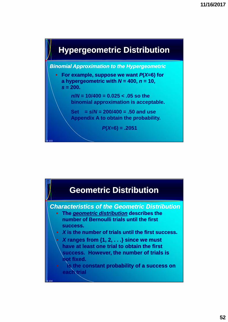
6-103
•• For example, suppose we wantFor example, suppose we want PP((XX==66) for) foraa hypergeometrichypergeometric withwith NN == 400400,, nn == 1010,,ss == 200200..
n/N = 10/400 = 0.025 < .05 so thebinomial approximation is acceptable.
Setp= s/N = 200/400 = .50 and useAppendix A to obtain the probability.
Binomial Approximation to theBinomial Approximation to the HypergeometricHypergeometric
6-104
•• TheThe geometric distributiongeometric distribution describes thedescribes thenumber of Bernoulli trials until the firstnumber of Bernoulli trials until the firstsuccess.success.
•• XX is the number of trials until the first success.is the number of trials until the first success.•• XX ranges from {ranges from {11,, 22, . . .} since we must, . . .} since we must
have at least one trial to obtain the firsthave at least one trial to obtain the firstsuccess. However, the number of trials issuccess. However, the number of trials isnot fixed.not fixed.
Geometric DistributionGeometric Distribution
Characteristics of the Geometric DistributionCharacteristics of the Geometric Distribution
•• ppis the constant probability of a success onis the constant probability of a success oneach trialeach trial
11/16/2017
53
6-105
The geometric distribution is always skewed to the right.The geometric distribution is always skewed to the right.ParametersParameters pp= probability of success= probability of successPDF P(x) = π(1π)x1
Range X = 1, 2, ...Mean 1/πSt. Dev.
Comments Describes the number of trials before thefirst success. Highly skewed.
2
1
The mean and standard deviation are nearly the sameThe mean and standard deviation are nearly the samewhenwhenppis small.is small.
Geometric DistributionGeometric Distribution
Characteristics of the Geometric DistributionCharacteristics of the Geometric Distribution
6-106
•• At Faber University,At Faber University, 1515% of the alumni make a% of the alumni make adonation or pledge during the annualdonation or pledge during the annual telefundtelefund..
•• What isWhat ispp??
•• What is the probability that the first donationWhat is the probability that the first donationwill not come until thewill not come until the 77thth call?call?
pp= .= .1515
•• The PDF is:The PDF is: PP((xx) =) =pp((11––pp))xx11
P(7) = .15(1–.15)71 = .15(.85)6 = .0566
Geometric DistributionGeometric Distribution
Example:Example: TelefundTelefund CallingCalling
11/16/2017
54
6-107
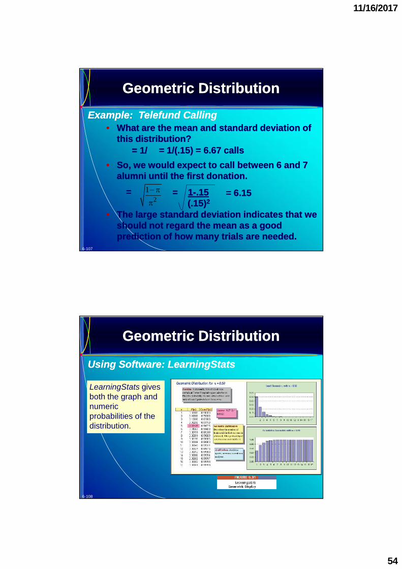
•• What are the mean and standard deviation ofWhat are the mean and standard deviation ofthis distribution?this distribution?mm== 11//pp
•• So, we would expect to call betweenSo, we would expect to call between 66 andand 77alumni until the first donation.alumni until the first donation.
== 11/(./(.1515) =) = 66..6767 callscalls
ss==2
1
== 66..1515== 11--..1515
(.(.1515))22
•• The large standard deviation indicates that weThe large standard deviation indicates that weshould not regard the mean as a goodshould not regard the mean as a goodprediction of how many trials are needed.prediction of how many trials are needed.
Geometric DistributionGeometric Distribution
Example:Example: TelefundTelefund CallingCalling
6-108
LearningStats givesboth the graph andnumericprobabilities of thedistribution.
Geometric DistributionGeometric Distribution
Using Software:Using Software: LearningStatsLearningStats
•• AA linear transformationlinear transformation of a random variableof a random variable XXis performed by adding a constant oris performed by adding a constant ormultiplying by a constant.multiplying by a constant.
Rule 1: maX+b = amX + b (mean of a transformedvariable)
Rule 2: saX+b = asX (standard deviation of atransformed variable)
Transformations of RandomTransformations of RandomVariablesVariables
Linear TransformationsLinear Transformations
11/16/2017
56
6-111
Rule 3: mX+Y =mX +mY (mean of a two randomvariables X and Y)
Rule 4: sX+Y = (standard deviation of sumif X and Y are independent)
Transformations of RandomTransformations of RandomVariablesVariables