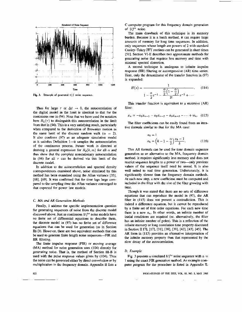
Discrete simulation of colored noise and stochastic processes … · · 2008-05-25Discrete...

Discrete Simulation of Colored Noise and Stochastic Processes and llf" Power Law Noise Generation

~ ~

N. JEREMY U S D I N , MEMBER, IEEE

This paper discusses techniques for generating digital sequences of noise which simulate processes with certain known properties or describing equations. Part I of the paper presents a review of stochastic processes and spectral estimation (with some new results) and a tutorial on simulating continuous noise processes with a known autospectral density or autocorrelation function. In defining these techniques for computer generating sequences, it also defines the necessary accuracy criteria. These methods are compared to some of the common techniques for noise generation and the problems, or advantages, of each are discussed. Finally, Part I presents results on simulating stochastic differential equations. A Runge-Kutta (RK) method is presented for numerically solving these equations.

Part I1 of the paper discusses power law, or 1/ f a, noises. Such noise processes occur frequently in nature and, in many cases, with nonintegral values for a. A review of 1/ f noises in devices and systems is followed by a discussion of the most common continuous 1/ f noise models. The paper then presents a new dim1 model for power law noises. This model allows for very accurate and efficient computer generation of l /f" noises for any a. Many of the statistical properties of this model are discussed and compared to the previous continuous models. Lastly, a number of approximate techniques for generating power law noises are presented for rapid or real time simulation.

I. INTRODUCTION

The need for accurate simulation of stochastic processes and stochastic differential equations arises across almost all disciplines of science and engineering. Mechanical and aerospace engineers often simulate complex, nonlinear models of dynamic systems acted upon by noise. In electrical engineering and physics it is common to simulate various types of colored noises as models for sensors and actuators. There are numerous nonlinear systems arising in all areas of physics that require techniques for simulating stochastic differential equations. And the timing community has a long history of simulation for modeling phase and frequency noise in oscillators [2], [4], [5], [8],

Manuscript received August 9, 1993; revised January 30, 1995. This work was supported by NASA Contract NAS8-36125.

The author is with the W. W. Hansen Experimental Physics Laboratory, Relativity MissiodGravity Probe B, Stanford University, Stanford, CA 94305-4085 USA.

IEEE Log Number 9410317.

[lo], [121-[14], [271, 1341, P71, [391, [411, [441, [531, [541, [571, [581, [@I, 1681, [@I, [731-[751, [771, [791.

This paper discusses the theory and mechanics of generating digital, pseudorandom sequences on a computer as simulations of known stochastic processes. In other words, given the autospectral density or autocorrelation of a process or a differential equation describing a system, methods are presented for producing digital sequences with the "correct" discrete spectrum or correlations. The precise meaning of correct is discussed but can vary depending upon the specific application. Though many new results are reported, particularly in the area of nonlinear differential equation integration and power law noise simulation, this paper is also intended as a tutorial on colored noise analysis and generation. Thus the detailed proofs or derivations are omitted or referred to cited works.

The paper is divided into two parts. The first discusses the general problem of simulating stochastic processes on a computer. Some time is spent defining what is meant by a stochastic simulation and criteria are presented for evaluating the effectiveness of a generation method. Some past techniques, particularly those involving direct simulation in the frequency domain from given spectra, are reviewed with an eye toward pointing out some of their deficiencies. Part I presents two techniques for simulating noise with a given spectra or autocorrelation function-a time domain and frequency domain method. In addition, a RK algorithm for simulating general, nonlinear, inhomogeneous stochastic differential equations is reviewed.

The second part focuses on the problem of generating sequences of power law or l / f " noises (also often called fractal processes). This is a remarkably ubiquitous problem spanning innumerable fields, from music and art to hydrology and low temperature physics. Countless devices and systems have been seen to produce noises with an autospectral density proportional to f-" with f the cyclic frequency and a a real number between 0 and 2. Many models and techniques have been proposed in the past to simulate these noises. Because the spectrum is not rational, it is impossible to use standard linear system

0018-9219/95$04.00 0 1995 IEEE

PROCEEDINGS OF THE IEEE, VOL. 83, NO. 5 , MAY 1995 802

-

theory and differential equation models to simulate the noise via the techniques in Part I. Thus in Part 11, after a review of past generation techniques, a new model is proposed. This model, first proposed by Hosking [31] and later independently by the author, can be used to generate digital sequences of l/fa noise. The properties of this model are discussed in some detail as well as the advantages it has as a generating mechanism over previous methods. In particular, it can be used over a frequency band of arbitrary size and it is strictly scale invariant.

Because noise simulation spreads over so many diverse disciplines, it is difficult to find a notation agreeable to all participants. This paper, therefore, uses common engineering notation and methodology for the stochastic process and system theory discussions. This notation is consistent with that used in [9], [14], [33], [52], [62]. Discussions of discrete system theory and the a-transform can be found in [231, 1511, [521.

PART I: STOCHASTIC PROCESS SIMULATION

11. REVIEW AND DEFINITIONS

Before embarking on the detailed discussion of noise simulation, it is useful to review some fundamentals of stochastic process theory and noise measurements. This section presents background information and definitions as well as some new, and important, results in stochastic process analysis and spectral measurement and estimation that will form the foundation for the simulation techniques discussed in Section 111. The review material in this section follows the presentation in [52]. Further reading can be found in [9], [26], [62], [70], [74]. Much of the information on spectral density measurements and estimation can also be found in [9].

A. Stochastic Processes It is assumed that the reader is familiar with the funda-

mental axioms of probability and basic random variables. If we are given the probability space ( R , 7 , F), then the stochastic process z ( t ) is defined in [52] as follows:

"z( t , C) is a stochastic process when the random variable z represents the value of the outcome < of an experiment 7 for every time t," where R represents the sample space, 7 the event space or sigma algebra, and F the probability measure [26].

Normally, the dependence upon the event space, C, is omitted and the stochastic process is written as z(t) . If the probability distribution function for z is given by F ( z ) , then we can define the general nth order, time-varying, joint distribution function, F(z1,. . . , z,; tl, . , tn) , for the random variables z ( t l ) , . . . , z(tn). The joint probability density function is then given by

In most cases, and all those in this paper, only the first and second order properties of the process are desired rather than the complete joint distribution function. For Gaussian processes, these second order properties completely define the process distribution. These properties are defined via the following equations:

J -00

where q is the mean value of the process and the notation E{ } refers to the expected value operation taken over the ensemble of processes {z(t , C)}.

The two-time autocorrelation of the process is given by

The autocovariance is defined by

(Note that all processes in this paper are real). Thus, the variance of the process, a2(t) , is given by

C( t , t). For this paper, all processes will be assumed zero mean so that the autocorrelation and autocovariance are identical.

In general, the moments of a stochastic process defined in (2) and (3) vary with time. However, a stationary process is defined as one whose density function is invariant to time shifts and thus independent of the times t l , t z , . . . , t,. Such a process is called strict-sense stationary. A wide- sense stationary process is one whose first and second order properties only are independent of time, that is, q(t) = q,

For stationary processes the autocorrelation function def- and R(t1,tz) = R(t1 - t z ) .

inition is often written in the asymmetric form:

The variance of the process is then given by R(0). Since we will be dealing with many nonstationary and

transient processes, it is more convenient to use a symmetric definition of the autocorrelation function:

For stationary processes, (6) and (5) give the same result. However, when we later compute spectra and other properties of nonstationary processes, (6) will be necessary in order to achieve consistent and accurate results.

This distinction is important as we consider noise generation. In simulation, we must be concerned with the transients of processes, thus implying that all signals under consideration for simulation will be nonstationary. How- ever, we can define an asymptotically stationary process as

KASDIN DISCRETE SIMULATION OF COLORED NOISE AND STOCHASTIC PROCESSES

~ - __ - ~~

803

one whose autocorrelation function satisfies:

lim R ( ~ , T ) = R(T). t+m

(7)

Many of the process models used for simulation will be asymptotically stationary.

Lastly, it is useful to have a measure of the “memory” of a process. The correlation time, for a zero mean process, is defined in [52]:

B. Example Processes Introduced here are three fundamental stochastic pro-

cesses. These processes form the basis of all the analysis and simulation that follows.

1) Markov Process: The first process of interest is the exponential correlation (or first-order Markov) process (often called low pass white noise for reasons we will see later). This process is stationary and zero mean with autocorrelation function:

This process has a correlation time, by (8), of a. 2 ) Brownian Motion: The second, and immensely impor-

tant, process is the Wiener process or Brownian motion. Brownian motion was first experimentally discovered in 1827 by Robert Brown when he observed the erratic motion of particles trapped in the pollen of plants which resulted from the interaction of the particles with the molecules of the liquid. The first rigorous and quantitative analysis of Brownian motion was performed by Albert Einstein in 1905, where he presented the first estimate of Avogadro’s number. Later, P. LRvy and N. Wiener developed a more mathematical treatment of the associated stochastic process [29]. Here, only a brief introduction to Brownian motion is presented. A good mathematical description of the process can be found in E291 and a more general discussion in [30],

The Brownian motion process, B(t) , is defined as a zero mean stochastic process that satisfies the following three properties [30], [52]:

[521.

a) B(0) = 0. b) B( t ) - B(s) is stationary and normal with mean 0

and variance cx It - S I for s 5 t.

are independent for tl 5 tz 5 . . . t,. c) B(t2) - B(tl), B(t3) - B(t2), “ . 7 B(t,) - B(tn-1)

Properties b) and c) are often used to point out that the process has independent and stationary increments. These three properties can be used to derive the autocorrelation function for Brownian motion [30], [52]:

(10) min(t, s) for t , s > 0

for t , s 5 0 RB(t, s) = { where Q is a constant of proportionality in definition b.

804

It is straightforward to show from this that Brown- ian motion is a nonstationary process with symmetric autocorrelation:

RB(t,r) = Q(1- 7) . Using (8) it can be seen that the correlation time of

Brownian motion is undefined. Frequently, Brownian motion is said to have infinite memory-that is, it retains correlation with values infinitely far back in time.

Papoulis [52] has an alternative derivation of the Wiener process as the continuous time limit of a random walk. A random walk is defined as a discrete step .process where at each time step At the value of the process is increased or decreased (with probability 1/2) by a fixed amount. In the limit as At + 0 the Wiener process is formed and can be shown to satisfy the three properties above. For this paper, it is more convenient to use the conventional continuous definition above with the random walk being derived, in Section 111, as a discrete approximation of Brownian motion in order to simulate it.

3) White Noise: The last process of interest is the derivative of the Brownian motion-white noise. The concept of white noise arose as Langevin tried to develop a dynamical description of Brownian motion [74]. The result was a first order linear differential equation driven by a white noise process (that is, a process with uniform spectral density) known as the Langevin equation. In order to produce pure Brownian motion (with no retarding term), white noise then becomes defined as the derivative of Brownian motion [26], [301, [521, W21, [701, W I :

a d w(t) = -B(t) d t

or, alternatively, Brownian motion becomes modeled as the integral of white noise.

Unfortunately, this definition raises some difficulties as the Wiener process is everywhere nondifferentiable. This implies that white noise does not exist as a stochastic process by itself, which will be evident when we examine its second order properties. Rather, white noise as defined in (12) is given meaning by its behavior as a functional in stochastic integrals of the form:

lb f ( t ) w ( t ) dt = f ( t ) dB(t). (13) lb The stochastic integral in (13) can be defined in a number of ways. The most common definition is due to Ito and the resulting integral is known as the Ito integral. In essence, the Ito definition provides an interpretation of the integral in (13) that also results in the necessary Brownian motion properties when f ( t ) G 1. In addition, it allows certain stochastic processes to be modeled as linear systems that result in the measurable autocorrelation functions of Section 11-D. The drawback is that the usual rules of calculus (such

PROCEEDINGS OF THE IEEE, VOL. 83, NO. 5, MAY 1995

as the chain rule) must be modified for stochastic processes’ [301, [701, [741.

While the It0 equation will be discussed a bit further in Section IV when simulation of general nonlinear stochastic differential equations is discussed, it is beyond the scope of this work to discuss the details and subtleties surrounding white noise and the definitions of stochastic integration and differentiation. Excellent discussions can be found in [30], [70], [74], [75]. For the purposes here, white noise can be treated as a stochastic process with second order properties that result in solutions of integrals such as (13) consistent with the rules and properties of the It0 calculus and that, upon integration, result in a Brownian motion satisfying the previous definition. We must only remember that white noise does not exist as a bona fide physical process but only as an intermediate tool to the solution of stochastic integral and differential equations. This will prove very useful in Section I11 as we model and simulate stochastic processes.

Following this procedure, it can be shown that white noise can be interpreted as a zero mean stochastic process with values w(ti ) and w ( t j ) that are uncorrelated for every ti and t j # t; [52]. The autocorrelation of white noise can then be taken as

where Q(t ) is an arbitrary scaling constant and 6 ( t ) is the Dirac delta function. Using the usual rules for the delta distribution, the correct properties of the Ito integral can be shown. This should come as no surprise-just as white noise is defined only by its behavior as a functional in integrals such as (13), so is the delta function defined [ 111. This also illustrates the difficulty in interpreting white noise as a process, since the delta function (and thus its variance) is undefined at zero. Note that stationary white noise has Q(t) = Q.

C. Spectra An additional measure of a stochastic process is the

autospectral density. The autospectral density (or simply spectral density)2 of a wide sense stationary stochastic process is defined by the Fourier transform of the autocorrelation function:

03

(15) s ( w ) = R(7)e-jW7 dT.

This holds as long as the autocorrelation is absolutely integrable:

A L 03

(16)

‘The other most common definition for the stochastic integral is the Stratonovich Integral. This definition has the property that the usual rules of calculus apply. Further properties of this definition will not be pursued in this paper.

2This is also often called the mean square spectral density or power spectral density.

Because R(r) is real and even, this can be simplified to the Fourier Cosine transform:

S(w) = 2 /U R(T) cos w r d r . (17)

Thorough discussions of the spectral density and its properties can be found in [9], [ l l ] , [12], [51], [521.

Using (17), the spectral density of the exponential correlation process can be computed:

The spectral density of stationary white noise is a constant, &. This lends apparent the name “white noise”-the process contains equal information at all frequencies.

The use of the spectral density as a description of a nonstationary process’s second order properties is more difficult. Equation (16) is not normally satisfied and thus the spectral density does not formally exist. This problem is significant since, as discussed earlier, most simulated processes are nonstationary unless we allow for decay of transients ([37] mentions a way to avoid this problem by careful selection of initial conditions). In addition, in Part I1 we will be generating power law noises (generalizations of Brownian motion) that are also always nonstationary. There has been some discussions [9], [46], [51] of the problem of defining the spectral density for nonstationary processes, but most fall short as a tool for developing simulation techniques.

This dilemma is resolved by examining the spectral measurement and estimation process. The true usefulness of the spectral density is in computing the second order statistical properties of a measured stochastic process. In addition, noise generation is frequently based upon the desire to simulate a process with a spectral density modeled after a measured one. Therefore, in the remainder of this paper, we consider only spectra obtained via Fourier analysis of measured signals (called the sampled spectrum or periodogram [9], [51], [52]). References [51] and [52] have discussions of other spectral estimation procedures, most based upon the use of an autocorrelation estimate (which is difficult to obtain in practice).

To derive the sample spectrum, first, the finite Fourier transform is computed for a segment of the process from to to to + T [91,

I have deviated from the standard here by allowing a time shift to such that the experimental data is an arbitrary segment from the given process (this, for example, allows us to wait for the decay of any transients).

An initial estimate of the spectral density is made via [9]:

A 1 S ( w ) = -\X(wIT)l2. T

KASDIN DISCRETE SIMULATlON OF COLORED NOISE AND STOCHASTIC PROCESSES

_ _ _

805

This estimate of the spectrum is both biased and in- consistent. In fact, the error in the estimate can be as large as 100% for all T. In practice, the variance in the estimate is reduced by averaging a large number, nd, of the estimated spectra from different segments of the process (see [9], [51], and [52] for more details on periodogram smoothing, spectral averaging, and windowing). Here, the estimate is made consistent by equivalently considering the expected value of (20). Using the definition of the symmetric autocorrelation function, a formula can then be found for the sampled spectrum of an arbitrary segment of a process:

S ( w ) e E { S ( w ) }

R(t ,r) dt e-iwr d 7 1 1

0 t , + T + ~ / 2

= L [ h L2 + 1’ [ R ( ~ , T ) dt e-jwT d7.

(21) Again, this formula differs from most standard texts because of the use of t, to allow arbitrary segments and the use of R(t, 7) to allow for nonstationary processes.

For an asymptotically stationary process (and thus large to), (21) reduces to [9]:

t , + T - ~ / 2

S ( W ) = E { S ( w ) }

(22) Note that this estimate is biased. However, for large T , the sample spectrum converges to the correct spectral density resulting in an asymptotically unbiased estimate. This bias, due to the finite length of the process, is addressed in more detail below.

Normally, the spectra of processes under consideration are presented based upon (15) or the linear systems tools presented in Section 11-D. However, the result in (21) c~ now be used to compute the expected sample spectrum, S, for any process, including nonstationary ones. For example, using the autocorrelation function given in (1 l), the spectral estimate for Brownian motion is computed to be

cos wT 2 - 2 - sin wT. (:) w2 Tw3

(23) For the usual discrete frequency steps, w = 2alc/T, or

for T much larger than to, this reduces to 2

W 2 S B ( W ) = -.

This spectral estimate was taken using the most convenient of windows-a rectangular one. However, it is known that such a time window can cause significant distortions to the spectrum, both at specific frequencies [9], [51],

[52] and as a broad-band bias [ S I . It is very common to use alternative time windows that improve the spectral estimate. For example, using a Hanning window [9] (with normalization 8/3) on the Brownian motion process, the new spectral estimate is (simplified for t, = 0):

S B ( W ) = -

80a4 - 24.rr2T2w2 + T4w4 + T 4 ( 4 a 2 / T 2 - w2)3

}. (25) 48.rr2Tw sin wT - 4T3w3 sin wT

+ T 4 ( 4 a 2 / T 2 - w ’ ) ~

For large T this converges to 1/w2. This difference is a surprising and very intriguing result

and particularly remarkable in that the error is precisely a factor of The obvious question is which represents the “true” spectral density of the Brownian motion? Since the formal spectral density of Brownian motion doesn’t exist, the better question is which provides the most accurate information about the second order properties and possible linear models (see Section 11-D) for Brownian motion?

No clear answer to these questions has been provided. However, consistency would suggest that the Hanning windowed result is closer to the “correct” estimate. One would expect that a nonnormalized Markov process should converge point-wise to the Brownian motion as the correlation time becomes very long (i.e., much longer than the time window of observation). This observation would suggest a 1/w2 form for the Brownian spectral density (see 18). This 1/w2 form also agrees with the transfer function model for Brownian motion when viewed as the integral of a white noise (see Section 11-D). It is this author’s belief that the factor of two in (24) is an error due to a broad-band bias introduced by the rectangular window.

The formula in (21) and the results that follow will prove to be very useful in the next section when we discuss linear systems.

D. Linear Systems For the majority of applications, including those in this

paper, the desired processes can be modeled by Gaussian white noise into a linear system. The advantage of this modeling approach is that the resulting system can often be easily converted into a form that allows digital simulation. Section I11 describes that process in detail. In this section, a brief review of linear system theory is presented.

The output process, z ( t ) , of a linear system driven by white noise is represented by the convolution integral:

z ( t ) = h(P)w(t - P ) d P (26) I’ where h(t) is the causal impulse response function of the system and w(t) is Gaussian white noise with

31t turns out that for power law noises described in Part II this bias changes with the power of the autospectral density.

806 PROCEEDINGS OF THE IEEE, VOL. 83, NO. 5, MAY 1995

autocorrelation function Q ~ ( T ) and the integration is defined in the sense of Ito.

Note that (26) differs slightly from the usual convolution integral that has limits of negative and positive infinity. While that definition makes computing the second order properties of stationary processes very convenient, it is of little value in noise simulation and modeling. A lower limit of minus infinity implies a noncausal system while an upper limit of infinity eliminates transient information necessary in any numerical implementation. Rather, the formula in (26) is a transient representation of a causal, realizable system [85].

Using (26) we can find an expression for the symmetric, nonstationary autocorrelation function for the linear system in terms of the impulse response h(t):

t 2 7 - 2 0

t 2 7 - 2 0

Because of the transient nature of the linear systems being considered, it is most convenient to use the Laplace transform of the system in (26) for computing spectra. Thus

X ( s ) = H ( s ) W ( s ) (29)

where H ( s ) is the transfer function of the system (the Laplace transform of the impulse response). The Laplace version of the spectral density is then given (assuming a spectral density for the white noise of Q):

S(s) = QH(s )H*(s ) . (30)

For stationary noises, the spectral density can be found by substituting j w for s in (30) (see, e.g., [9]):

S ( W ) = Q H ( j w ) H ( - j w ) . (31)

As an example, we examine the linear system description for the first-order Markov process. This system has impulse response and transfer function:

Using (27) the autocorrelation function of this process is

(33)

For large t , this process is asymptotically stationary with an exponential autocorrelation equal to that given in (9). The spectral density via (31) is the same as that given for the exponential process in (18). If instead we use the nonstationary transient form of the autocorrelation in (21), we find the spectral estimate:

e-' /"(a/T)(l - a2w2) cos wT + - 2e-'/"(a/T) sin wT + ae-2t,/a

( 1 + a2w2)

(1 + a"2) T 1

COS WT - - 2 ( 1 + e-2r /a ) ] } . (34)

Observe that for large T, where the process approaches stationarity, this spectrum converges to that in (18). This is true even when to = 0 and all the transient details are included in the sample spectrum computation.

Note that, operationally, we can perform the substitution in (31) even for nonstationary noises, despite the fact that the Fourier transform of the original autocorrelation does not exist and thus the spectral density has no meaning. The obvious question is whether the resulting function agrees with the computed spectral estimate via (21). Or, asked the other way, can we use the computed spectral density estimate from (21) to postulate a linear system model for the process with impulse response h(t) and transfer function H ( s ) even though that process is nonstationary (that is, h(t) represents an unstable or marginally stable system)?

The answer to that question is often yes, as can be seen by examining Brownian motion. From (12) Brownian motion is given as the integral of white noise. Its impulse response function is thus the unit step function and its transfer function is

(35)

From (27) the autocorrelation can be computed and shown to be the same as presented in (1 1). The spectral density, using (35), is thus:

1 H B ( S ) = -.

s

Q W 2

SB(W) = -.

This spectral density is the same as the computed spectral estimate using the Hanning window in (25). As discussed earlier, the spectral estimate with a rectangular window results in the correct form but with a factor of two bias Again, it is this analysis in part that supported the conclu- sion that the rectangular window result is biased. Only the windowed result, 1/w2, can be used for a consistent linear system model to produce a process with the correct second order properties. In summary, the spectral estimate, even of a nonstationary process, is, in many cases, a legitimate basis for formulating linear system models for the stochastic

KASDIN. DISCRETE SIMULATION OF COLORED NOISE AND STOCHASTIC PROCESSES

~ ~- -

807

process. This point will take on great importance in Part I1 of this paper when we develop models and generating techniques for power law noises.

E. Discrete Linear Systems For discrete linear systems, the convolution integral in

(26) is replaced by the discrete convolution sum:

systems here provided the tools for computer generation. The first few sections of Section I11 discuss first how to relate this discrete model to the continuous one and presents the proper criteria for evaluating accurate simulations.

111. DISCRETE, LINEAR SIMULATION

(37) e=o

where we is an independent and identically distributed (IID) noise sequence with autocorrelation Ewmwl = QJml. Note that, unlike white noise, w here is a well defined discrete time process.

Similarly to the continuous case, the discrete, symmetric autocorrelation function is given by

I kfmI2-l

or

f k-ml2--1

Here, for wide-sense stationary noises, the spectral density function, s d ( W ) , is the Discrete Fourier Transform (DlT) of Rd(m). Using the discrete linear system model and z-transform theory, this discrete spectrum is given by

where H ( z ) is the discrete transfer function or z-transform of the discrete pulse response hk.

The frequency spectrum is found by substituting ejwAt for z. References [9], 1231, [51], [52] have more details on the discrete spectral density calculation. It short, this involves computing the periodogram rather than the sample spectrum by using a sampled version of (19). It is shown in these references that this process, using the DFT, produces an accurate estimate of the expected sample spectrum in (21) (for bandlimited spectra and with the proper cautions about aliasing). In order to obtain the correct scaling to convert &(U) into an estimate of the continuous spectral density (implying that Rd(m) resulted from samples of an observed process) it is necessary to multiply s d ( W ) by At

The next section presents a detailed description of methods for simulating stochastic processes of the type described in Section 11. Essentially, the brief discussion of discrete

[91, [111.

A. Criteria and Dejnitions Before discussing in detail the mechanics of generating

digital sequences of colored noise, it is important to define the criteria for an accurate noise simulation. Since in this section only the linear system models described in Section I are considered, a mean square definition of a stochastic simulation is appropriate. This is done as Definition 1.

Dejnition I : A zero-mean, discrete, Gaussian stochastic process, X k l is said to “simulate” the continuous, Gaussian stochastic process, x ( t , <), if the discrete, symmetric autocorrelation function, Rd(k, m ) , is equal to samples of the continuous autocorrelation, R(t, T ) . That is,

& ( k , m ) = R(kAt, m a t ) . (41)

Since we are limiting ourselves to zero mean, Gauss- ian processes, it is a fact that a simulation that satisfies Definition 1 also has the property that the probability mass distribution of X k is equivalent to samples of the joint probability distribution of x ( t ) . Such a simulation will be called strict-sense. For cases where x ( t ) is non- Gaussian distributed such that only Definition 1 is satisfied but the probability distributions do not correspond, then the simulation will be called wide-sense. Kloeden and Platen [74] also point out these two possible ways to simulate the solution to a random differential equation of which the linear systems in Section I1 are special cases. There, they refer to the scrict-sense simulation as a strong simulation where a single member of the ensemble of random processes, { x ( t , <)}, is simulated. That is, the discrete simulation process is a sampled sequence from one of the (bandlimited) members of the ensemble { x ( t , <)}. Wide sense simulations, where only the first and second order properties of the process are reproduced, are referred to as weak simulations. Again, it is a fact that for Gaussian random processes these two approaches are identical. More will be said on this subject as well as on nonlinear stochastic differential equations in Section IV.

This distinction is more important than it may seem, as it is possible to generate many non-Gaussian processes that are quite different but have identical autocorrelation functions. An example in [12], [52] illustrates this, where the random telegraph signal (non-Gaussian) is shown to possess the same autocorrelation functions as a first order Gauss-Markov process. Also, many shot-noise processes have very similar statistics to the Gaussian counterparts with the same impulse response function but, for low arrival rates, can have very different probability densities [86]. This


paper only considers Gaussian processes or high rate shot noise processes that, by the central limit theorem, approach Gaussian distribution.

It is very important to point out here that satisfaction of Definition 1 is not equivalent to generating noise with a discrete autospectral density that samples the continuous autospectral density function. Many authors [ 101, [19], [S3], [67] have attempted noise generation by creating discrete random spectra (modeled as samples of the continuous one) and inverting the complex Fourier series to the time domain. This is a particularly attractive approach for processes with nonrational spectral density functions (such as l/f" noises). In fact, rarely is the autocorrelation available or even estimated in practice. Most often, the measured noise sequence is converted directly into a periodogram (via (20)), from which a continuous form is inferred.

This approach also seems justified as it is fairly straightforward to compute the moments of X ( f ) (the Fourier transform of x ( t ) ) . These are then used to randomize the frequency shaped spectral components X R ( f ) and X I ( f ) (see, for example, [lo], [19], [S31, [671).

This method of generation, however, ignores the distortions to the autospectral density produced by sampling and windowing. Returning to Definition 1, suppose a continuous autocorrelation function of a wide-sense stationary process, R(T), with corresponding spectral density, S(w), is sampled, resulting in &(mat). The resulting discrete autospectral density can then be found by taking the DFT of a length N segment of Rd(mAt). More commonly, the approach of Section 11-C is used to find the sampled spectrum. This discrete density function, Sd(w), only ap- proximates S(w) and approaches it exactly only as At ---f 0 and N * oc. The effects of windowing have already been discussed and exist even for continuous processes. There are two remaining distortions due to sampling effects and causality.

The sampling of R(T) to produce Rd(m) results in aliasing of the high frequency content below the Nyquist frequency (1/2At). That is, the spectrum of &(m) is periodic. The original function R(T) can be found from this sample only for perfectly bandlimited spectra, an impossibility in practice.

As discussed in Section 11-D, it is essential when generating noise that the system producing it be causal. This implies that the real and imaginary parts of the Fourier transform of the process (19) are a Hilbert transform pair.

In theory, it is possible to generate noise in the frequency domain by considering these effects when shaping the random spectral density. However, this is extremely difficult in practice. If, instead, the discrete spectrum is shaped based solely on the assumed continuous function, ignoring these distortions (as is frequently done in the literature), then the autocorrelation function of the resulting sequence after inversion will be distorted and not satisfy Definition 1.

The next sections describe more precise methods for generating noises that do not suffer from these problems. These techniques use the discrete linear system models

described in Section 11-E to produce noise sequences that simulate continuous processes. To do so, there are two questions that must be answered: 1) How does one find hk when given h( t ) (and thus R ( ~ , T ) ) , or, equivalently, S(w), of the continuous process, so that Definition 1 is satisfied? and 2) how can (37) be used to generate noise when hk is known?

B. Batch Frequency Domain Simulation We answer question (2) first and defer until the next

section a discussion of finding the proper hk. Here we assume that some hk is provided such that the autocorrelation in (38) is equivalent to samples of the continuous autocorrelation given by (27), as required by Definition 1.

The first, and most straightforward, method to generate the time sequence in (37) is to simply perform the discrete convolution; that is, treat (37) as a moving average (FIR) filter with an infinite number of coefficients. (It is important to perform linear convolution rather than circular convolution, that is, to assume that h k and W k are causal sequences with zero value for indices less than zero [Sl].) Though this technique benefits from being able to generate any number of points, it is extremely slow. Rather, it is more efficient to use the common practice of replacing convolution by multiplication in the frequency domain.

The convohition in (37) is implemented much more rapidly by multiplying in the frequency domain. Causality is assured by generating a zero-padded, IID sequence, wk, and a zero padded sequence of pulse response values, hk (guar- anteeing linear rather than circular convolution). These are then transformed, multiplied, and inverse transformed using commonly available FFT routines to produce the simulated sequence. The variance of the IID noise, Q d , is chosen to match amplitudes with the continuous autocorrelation function or, equivalently, an unbiased autospectral density estimate.

This technique's main drawback is its memory burden. Because it is a batch method, it can require large amounts of memory for long time sequences. In addition, only sequences whose lengths are powers of 2 can be generated in reasonable time. Section 111-D will describe the more efficient recursive algorithms for real time generation that can be applied to time-invariant linear systems.

Note the difference between this batch, frequency domain method and the direct one described earlier. In the references cited, the random spectrum was generated in the frequency domain directly. Here, the pulse response and white noise input are generated in the time domain first. Transformation to the frequency domain is only used to rapidly compute the convolution by replacing it with multiplication, taking advantage of the rapid FFT algorithms.

C. Selecting hk The second question asked above addresses how to select

the proper hk given h( t ) , R(t,.r), or S(w), to ensure that R(lc,m) is equal to samples of R(t,.r). In general there is no definitive formula or technique for choosing hk. In Part 11, for example, when l / f" noise is considered, an

KASDIN: DISCRETE SIMULATION OF COLORED NOISE AND STOCHASTIC PROCESSES 809

H ( z ) is postulated, an hk computed, and later they are shown to possess the desired properties.

It would be convenient if hk could be computed by sampling h(t) for the process being simulated; unfortunately, this is only true when H ( s ) is a rational function of s. This can be shown by discretizing the first half of (27) for T > 0. Sampling R(t,T) in (27) results in:

k-mI2-1 ( n + l p t

R(kat, mat) = Q / h(p )qp + mat) dp. n=O nAt

Let 17 equal p - nat:

R(kAt, mat) = Qk-m/f-llAt

n=O h(v + nAt)h(v + nAt + mat) dv .

(43)

In general, this cannot be solved for an h k to reproduce (39). For certain linear systems, however, with rational transfer functions (in particular, those with a single pole and no zero), it is true that h(t + T ) = h(t)h(.r). For this special case,

k-m/2-1

R(kat,mat)=Qd hnhn+m (4) n=O

where

hn = h(nAt) (45)

and At

Q d = Q I h2(v) dv. (46)

Thus it is here possible to simulate the colored noise (as per Definition 1) using the discrete convolution in (39) by simply sampling the continuous impulse response function and choosing the discrete IID noise variance using (46). For systems with irrational transfer functions or multiple poles and zeros, the discrete pulse response must be found by some other method (for example, that of Section 111-D below).

An alternative approach for many rational systems is to find hk by direct system identification 1371, [831, 1841. Here, R(k, m) is estimated from measured data (rather than assumed a priori) and the coefficients of an ARMA model are computed directly from the Yule-Walker equations (see Section 111-D). This avoids the need to assume a function for R(t, T ) or S(w) but does require the process to be well fit by an ARMA model.

D. Rational Spectra ana' Linear, Stochastic Differential Equations

As mentioned above, when H ( s ) is a certain rational function of s, hk can be found exactly by sampling h(t). However, there is an easier method for generating the

noise in this case. For linear systems with rational transfer functions, the output can be written as the solution of the following inhomogeneous, linear stochastic differential equation with constant coefficients:

( ( t ) =F<(t ) + G w ( t ) 4t) = C<(t) (47)

where w( t ) is a vector of white noise processes with spectral density matrix Q , H ( s ) = C(s1 - F ) - l G , and the order n of the matrix F is the same as the number of poles in a minimal realization of H(s ) . (There are many excellent books on linear systems that discuss this subject in much more detail. See, for example, 1121, [131,[221, [231, [33], [62]). Note that, as mentioned in Section 11-B, (47) is a special case of the nonlinear It0 stochastic differential equation that will be discussed in slightly more detail in Section IV.

Reference [36] has a derivation of RK type integration methods for simulating systems described by (47). However, while a numerical integration would produce a sequence with autocorrelation function only approximating the continuous one, in this linear case, the system can be solved exactly. The equations below show how to produce a sequence with autocorrelation exactly sampling the continuous one. Further discussion of R-K methods is deferred until Section IV.

References [52] and [74] discuss in some detail the properties of the autocorrelation function and autospectral density for solutions to the system in (47). It is also proven that samples X k of the process x ( t ) are guaranteed to have an autocorrelation that samples R(T). For brevity, these analyses will not be reproduced here. Instead, the equations below show how to solve (47) at the points 2 ( t k ) . 'The resulting sequence is thus a sampling of z ( t ) and therefore, by the proof in [52], satisfies Definition 1. Note that while these derivations can be performed in a very rigorous manner using the definition of the Ito integral (see, for example, [74]), here they will be solved using a more standard systems approach and the delta function description of white noise.

The solution to (47) can be found in many texts on linear systems [13], [33], [62]. This solution is given by

<(t) = @(t, O)<(O) + it @(t, ~ ) G ( T ) ~ ( T ) d~ (48)

where @(t, T ) is the state transition matrix and equals, for linear, rational systems, @ ( t ) @ - l ( T ) . @(t) is the solution of the matrix differential equation:

(49) d dt -@(t) = F(t )@(t ) .

Note that we have generalized (47) to include time varying systems where it is impossible to define a transfer function. For the time invariant case, @(t, T ) = @(t--7) and

@(t) = L - l { ( s l - F ) - l } eFt. (50)

810 PROCEEDINGS OF THE IEEE, VOL. 83, NO. 5 , MAY 1995

To develop a simple, recursive formula for noise generation, we solve (47) over an interval At to find:

For time invariant linear systems (51) and (52) simplify to

(53) t k + 1 = @(At )& f wk

and At

Q d = @(T)GQGTaT(T) dT. (54)

This equation for Q d can be solved using an algorithm due to Van Loen 1651. (See Appendix I) Note that this is the matrix equivalent of an ARMA model for the process. The matrix equation (53) can be converted into an ARMA time series using simple z-transform theory 1231, 1331, [51].

Equation (51) or (53) can be used for very fast and efficient noise generation to simulate noises given by rational transfer functions (and thus linear, time invariant differential equations) or by linear, time varying differential equations of the form (47).

E. Example Simulations I now return to the three sample processes and show

how the methods of the previous subsections can be used to simulate two of them: the Markov process and Brownian motion. Because white noise is undefined in practice (it has an infinite variance) it is not possible to simulate it. How- ever, the next section will discuss useful approximations for simulating uncorrelated measurement noise.

The first order Markov process given in (32) can be represented by the stochastic differential equation:

i + bx = bw(t) (55)

where b = l /a. This can be discretized, for a time step At, using (48)-(54) to the following difference equation:

(56) - A t l a xk+l = e xk + W k

where W k is an IID process with variance:

This difference equation is then very easily simulated on a computer using any standard pseudorandom number generator and normal distribution algorithm.

We can also examine the discrete autocorrelation and spectral density of this discrete process. The autocorrelation can be found by substituting the pulse response for (56),

Spectral Density of Continuous and Discrete uarkov Roccss

IO' 100 10' 102 1041 ' ' " ' " " ' ' " " " ' ' ' " " " ' ' * , , , - .

10 * Frequency (ridsec)

Fig. 1. Spectral density of continuous (solid) and discrete (dashed) Markov process.

h k = e C k A t f a , into (39). The result is found using standard formulas for finite sums:

Upon substituting for Q d from (57), this becomes

I . (59) &(k,m) = -[[e Q -mAt /a - e - 2 k A t / a

2a

Equation (59) is precisely equal to samples of the continuous autocorrelation for the first order Markov process as given in (33). Thus the discrete process satisfies the fundamental requirement of Definition 1 for an accurate simulation.

Finally, the discrete spectral density can be found most easily via (40) by squaring the transfer function of (56):

The resulting spectral density is

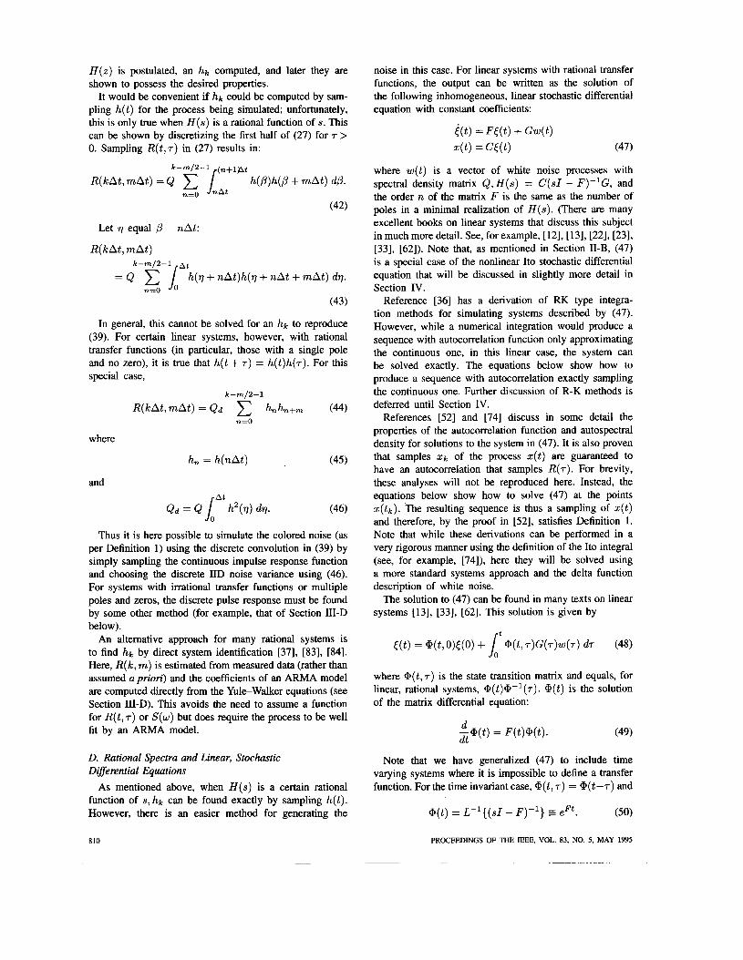
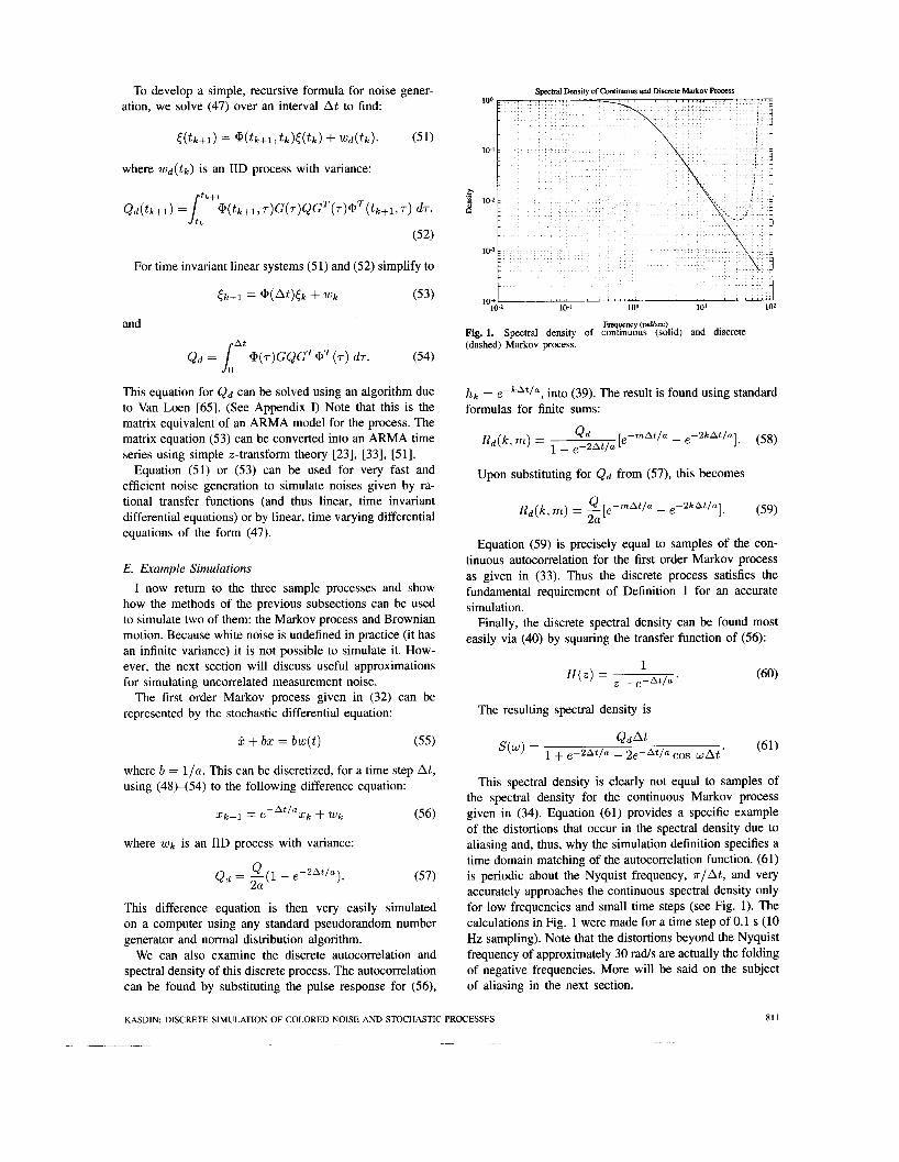
This spectral density is clearly not equal to samples of the spectral density for the continuous Markov process given in (34). Equation (61) provides a specific example of the distortions that occur in the spectral density due to aliasing and, thus, why the simulation definition specifies a time domain matching of the autocorrelation function. (61) is periodic about the Nyquist frequency, r /A t , and very accurately approaches the continuous spectral density only for low frequencies and small time steps (see Fig. 1). The calculations in Fig. 1 were made for a time step of 0.1 s (10 Hz sampling). Note that the distortions beyond the Nyquist frequency of approximately 30 rads are actually the folding of negative frequencies. More will be said on the subject of aliasing in the next section.

KASDIN, DISCRETE SIMULATION OF COLORED NOISE AND STOCHASTIC PROCESSES

~- .. ~

811

Brownian motion can be discretely modeled in a similar way. Here, we will use a slightly different approach and take the direct integration of white noise and convert it into a sum:

This can be written as a difference equation:

x k + 1 = xk -k w k

where W k is an IID process with variance &At. This is the standard random walk formula [52].

We can take the z-transform of (63) to find the discrete transfer function:

(63)

This results in the spectral density:

Again, the spectral density for a random walk is periodic and does not sample the Brownian motion function. However, for low frequency, this approximately equals:

This is the desired form of the spectral density given by (36).

F. Sensor Noise, Aliasing, and Prejiltering Finally, a few words should be said about the aliasing

phenomena seen in the last section. All of the approaches to simulation above have contained a hidden assumption-that the simulated discrete process includes the integrated effect of the noise acting upon the linear system during the simulation time step. This is significant and important when the simulation is modeling a dynamic system with random inputs described by a set of stochastic differential equations (that is, a driven linear system). In that case, an accurate representation of the state of the system at each time step is desired including the action of all inputs during the interval.

This is not true when modeling sensor noise. Frequently, the goal is to simulate the sampling of a measured random process with a given spectral density or autocorrelation. In that case, the integrated effect of driving noise on the model described in Section 111 is equivalent to aliasing the sampled process. That is, if we directly sample the continuous autocorrelation function then the resulting discrete spectral density is given by [9], [23], [51], [52]:

where w, is the sampling rate of 27tlAt. The discrete spectral density includes contributions from all the shifted

812

spectra due to aliasing. This accounts precisely for the distortions in the spectra seen in Section 111-E. In fact, numerical calculation of (67) using the continuous spectral density for the first order Markov process exactly repro- duces (61).

Normally, aliasing is avoided during measurements by first prefiltering with a high order low pass filter. To correctly simulate the desired process including sampling, the prefilter must be added to the linear system model before applying the methods of this section. This would, for example, remove the increase in the spectral density of (61) near the Nyquist frequency.

We can now approximately simulate a measured “white noise” process. If the process being measured has a very high frequency bandwidth compared to the sample rate, then the resulting sampled sequence can be well approximated by an uncorrelated IID process. If we assume a very sharp cutoff analog prefilter, then the variance of the noise can be easily computed. For a perfectly rectangular filter (noncausal and impossible in practice) with cutoff at the Nyquist frequency, the autocorrelation function is

Thus the variance of the approximate white noise process is given by R(0) or Qd = & / A t . We can also compute the variance for a realizable filter. For example, an Mth order Butterworth filter has spectral density:

where B is the filter cutoff frequency, or Nyquist frequency, of 1/2At. The discrete variance can then be computed via ParseVal’s Theorem [9] by integrating the spectral density in (69) to find:

For high order filters (large M ) , this is well approximated by the same result as the perfect low pass filter, Qd = &I A t .

Iv. NUMERICAL INTEGRATION OF STOCHASTIC DIFFERENTIAL EQUATIONS

A. Introduction It was mentioned in Sections I1 and 111 that the linear

systems described there were special cases of the more general, nonlinear Ito stochastic differential equation:

d dt - X ( t , C) = F ( X ( t , C), t ) + G ( X ( t , Cl, t ) w ( t , Cl. (71)

In this section the problem of simulating the solution to (71) is addressed. Unlike in the previous section, where the simulation was intended to generate sequences with second order properties that reproduced those of the process being modeled, here, (71) is assumed a priori as a model of the dynamics of a system driven by noise. The objective is to


numerically “solve” the stochastic differential equation as a simulation of the modeled system.

The stochastic differential equation (71) commonly oc- curs throughout science and engineering, most frequently as a dynamic model of a physical system driven by random forces or an electrical network with random voltage or current inputs. Again, one of the earliest forms was the Langevin equation used to describe Brownian motion [74], [75]. Before looking at simulation methods, it is worth briefly asking what is meant by (71) and how an a priori determination of such an equation may come about. There are two interpretations of the Ito equation given in (71). The first is simply as a stochastic differential equation driven by white noise as described in Section 11. There are two sources of this interpretation. The first is in using the linear form of (71) to model stochastic processes with known (or determined) autocorrelation functions (or spectral density). The Ito interpretation of white noise and corresponding solution can be used to create processes with the desired second order properties (autocorrelation and autospectral density). Secondly, equations of the form in (7 1) are often derived directly through dynamic descriptions of systems driven by random forcing functions. If these functions are considered to be independent processes, then in the continuous limit it is natural to assume a differential equation driven by white noise. Such equations arise in mechanics and electrical engineering extremely often and are the basis for much of modern control theory.

There is an altemative interpretation of (71) due primarily to Wong [70]. In contrast to the above Ito description, the white noise driving term is considered as an approximation of a very wide band but smooth process. In this case, the differential equation can be solved exactly for each sample path of the smooth process using classical calculus. Unlike the solutions above, which are nowhere differentiable due to the white noise, here the resulting sample paths are smooth. The obvious question is whether the solution to such an equation converges to the It0 solution of (71) as the low-pass driving noise approaches white. The Wong-Zakai theorem shows that process does converge to the solution of a stochastic differential equation, but in the sense of Stratonovich rather than Ito [74]. That is, a correction term must be added to (71) for an It0 solution to be equal to the convergent sample paths of the approximation [74], [75]. In other words, the Stratonovich interpretation of (7 1) is more appropriate when the white noise is taken as an idealization of a smooth, wide band noise process [74]. Grigoriu [77] has some discussion of the Wong-Zakai theorem and uses it to simulate stochastic processes under this interpretation but with only a simple Euler integrator.

It is interesting to point out that in the vector formulation of (71), the second interpretation can be converted to the first by the use of linear filtering. That is, rather than idealize the bandlimited process by white noise, it is reproduced by the methods of Section I1 using a linear It0 model driven by white noise. This is then added to the vector system in (71) to produce a larger It0 differential equation driven by white noise. Such an approach provides a link between the

Stratonovich interpretation of Wong and the more common (and useful) Ito interpretation. Wong and Hajek [70] have some discussion of the vector solution, but it is an open question whether the It0 solution of this larger system is the same as the Stratonovich solution (It0 system with correction term) of the smaller system.

As mentioned, the linear systems methods in Section I1 and the remainder of this paper examine only the It0 interpretation of (71). This is primarily due to the convenient treatment of white noise by a delta function and the many useful mathematical properties of the It0 equation. In addition, it is the Ito interpretation that is typically used in the control and dynamics work using stochastic differential equations. Should the interpretation of Wong and Zakai be more appropriate for a particular problem, the Stratonovich equation can be converted to an Ito one using the correction term described in [70] or [74] or the system can be augmented as described above.

It is beyond the scope of this paper to delve into the subtleties and mathematical details of stochastic differential equations. There is a large body of work on the properties and solutions of It0 (and Stratonovich) differential equations of the form in (71). The reader is directed to [61], [70], [73], [74] for examples of such treatments. Rather, this section expands upon the generation methods of the previous sections to examine techniques for simulating nonlinear stochastic differential equations. In particular, some recent work on a RK numerical solution approach is summarized. A detailed discussion and derivation of this technique is in [36].

There are many commercial packages available for simulation of dynamic systems described by continuous differential equations. Many now use graphical, block diagram interfaces for building the simulation. These packages must be used with care, however, on systems with random inputs such as that in (71). None of the available packages correctly accounts for the randomness in their solution methods. There are two main difficulties: 1) how to evaluate in real time the accuracy of the solution and, if possible, perform step-size control and 2) how to pick the mean and variance of the random input sequence to satisfy some appropriate criteria (see [58]) . To avoid these difficulties, the problem is often simplified in two ways. Sometimes, a simple, first order Euler integration is performed, because the properties of this integrator are easily examined and the driving noise covariance matrix is easily computed to be QD = &/At (this is directly related to the result for bandlimited white noise in Section 111-F). More frequently, a higher order method is used but with only a single call to the input noise generator per step. That is, while there may be numerous function evaluations to compute a single integration step (F(X, t) and G ( X , t) above), the input noise is only computed once at the beginning of the step and given the Euler value, &/At. This is equivalent to a zero order hold on the input noise and is particularly convenient when using commercial simulation software that allows external inputs to be applied to a block diagram simulation. This second approach is referred to as the “classical”


method in [36]. It is shown there that, independent of the order of the integration method, accuracy is lost by using this approach for the input noise.

It is not hard to see that most standard variable step and multistep methods are inappropriate for stochastic simulation. Multi-step methods rely upon assumptions regarding the smoothness of the solution-assumptions that are incorrect for the random sample sequences (recall that sample processes of the solution set of (71) are nowhere differentiable). In addition, the local error criteria normally used for determining step size variation do not apply to a stochastic simulation as a very accurate solution can still have large changes between steps, even for small step size.

References [73] and [74] have excellent discussions of both implicit and explicit solution methods for stochastic differential equations, both strict-sense and wide-sense. These methods, however, are exclusively low order Taylor series approaches. For more complicated systems it can be very unwieldy to find the Jacobian and higher order derivatives of the functions in (71). Reference [36] therefore presents an explicit, single-step, RK method for numerically solving (71). At present, the derivation has been performed only for the linear version of (71) where closed form solutions for the covariance exist. It is believed that under certain restrictions the same method can be generalized for nonlinear systems.

Before presenting the method, however, it is necessary to slightly modify Definition 1. Recall that for linear, Gaussian systems strict and wide sense simulations are the same. However, for nonlinear systems described by (71), this is no longer true and it is difficult, if not impossible, to derive an autocorrelation function in general. It is possible, however, to describe the time-varying covariance of the solution, X ( t , < ) , of (71). (See [36], [61] for a clear description of the Fokker-Planck equation used to derive the covariance solution). While in [74], [75] both strict and wide sense solutions are discussed, this work only examines wide sense methods. Current research is directed at strict-sense RK simulations.

Therefore, for general nonlinear or time varying systems we use the restricted Definition 2 for stochastic simulation.

Dejnition 2: A zero-mean, discrete stochastic process, X k , is said to "simulate" the continuous stochastic process given by (71), X ( t ) , if the discrete covariance matrix, Pk, is equal to samples of the continuous covariance matrix, P( t ) , within the error of the integration routine. That is,

The most general linear form of the stochastic differential equation is given by [74], [75]:

d - X ( t ) dt = ( F ( t ) X ( t ) + a@)) + G(t )w( t )

The differential equations for the mean and covariance of (73) can be found using the It0 formula for the chain rule [74]:

d dt -m(t) = F(t)m(t) + a ( t )

m d dt -P = F( t )P + PF(t)T + Bl(t)PB"t)T

1=1

+ a(t)m(t)T m + m(t)a(t)T + G(t)QG(t )T

+ (t)m(t)QIT G" t)T 1=1

+ Gl ( t )Q'm(t)TBl ( t )T ) . (74)

It is more common to examine linear equations without the driving term a ( t ) (zero mean) and without the bilinear matrix term B(t) . It is this form that is worked in this paper and in [36]. For these linear stochastic differential equations, as given by (47), the covariance matrix solves the matrix differential equation [14], [36], [61], [62]:

P ( t ) = F( t )P( t ) + P( t )F( t ) + G(t )Q( t )GT( t ) . (75)

Though it will not be studied in this paper, it is possible to develop a more general expression for the covariance using the Fokker-Plank equation for the nonlinear system in (71). This equation is [36], [61]:

P ( t ) = E { F ( X ( t ) , t ) X T ( t ) } + E { X ( t ) F T ( X ( t ) , t ) } + E { G ( X ( t ) , t ) Q ( t ) G T ( X ( t ) , t ) ) . (76)

The next section presents a RK algorithm for solving (71) such that Definition 2 is satisfied.

B. Runge-Kutta (RK) Solution Method The'RK method is a simple, and probably the most

commonly used, single step numerical integration routine for solving differential equations. There are many different RK type routines of different orders available. The general RK integration algorithm is given as follows:

If z(t) is the solution of the differential equation,

4 t ) = f(z, t ) (77)

then z(t) is simulated at time t k + l by the following set of equations:

zk+l = z k + aik i + azkz + . . . + a&, kl = h f ( t k , z k )

kj = hf t k 4- C j h , z k + ajiki)

j - 1

(78) ( i= l

where h is the step size. These equations are an order n RK integrator. The

coefficients ai, c i , and aji are chosen to ensure that z k

simulates the solution z(t) to order hn+l. That is,

z ( t k ) = zk + o(hn+'). (79)

The coefficients in (78) are found by Taylor expanding both (77) and (78) to order h" and matching coefficients.


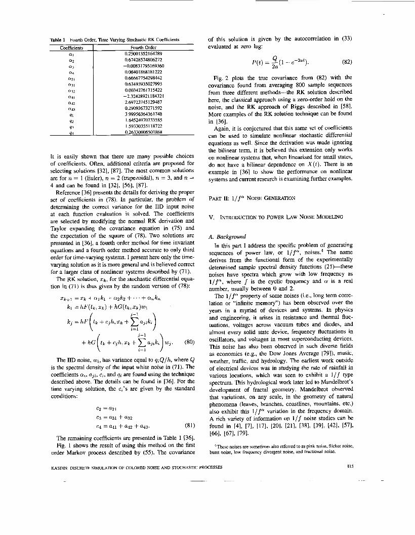
Table 1 Fourth Order, Time Varying Stochastic RK Coefficients

f f l 0.25001 352 164789 a2

a 3

ff4

ff2l

ff31

0.32

f fd l ff42

a 4 3

91 92 4 3

0.67428574806272 -0.OO831795169360 0.08401 868 18 1222 0.66667754298442 0.63493935027993 0.00342761715422

2.69723745 129487 0.29093673271592 3.99956364361748 1.64524970733585 1.593303551 18722 0.26330006501 868

-2.32428921 184321

It is easily shown that there are many possible choices of coefficients. Often, additional criteria are proposed for selecting solutions [32], [87]. The most common solutions are for n = 1 (Euler), n = 2 (trapezoidal), n = 3, and n = 4 and can be found in [321, [561, [871.

Reference [36] presents the details for deriving the proper set of coefficients in (78). In particular, the problem of determining the correct variance for the IID input noise at each function evaluation is solved. The coefficients are selected by modifying the normal RK derivation and Taylor expanding the covariance equation in (75) and the expectation of the square of (78). Two solutions are presented in [36], a fourth order method for time invariant equations and a fourth order method accurate to only third order for time-varying systems. 1 present here only the time- varying solution as it is more general and is believed correct for a larger class of nonlinear systems described by (71).

The RK solution, xk, for the stochastic differential equation in (71) is thus given by the random version of (78):

2 ~ + 1 = x k + ~ r l k l + a2k2 + . . . + ank, k i = hF(tk, x k ) + hG(tk, xk)wi

The IID noise, wi, has variance equal to qiQ/h, where Q is the spectral density of the input white noise in (71). The coefficients ai, aj;, ci, and qi are found using the technique described above. The details can be found in [36]. For the time varying solution, the ci's are given by the standard conditions:

c2 =a21

c3 =a31 + a32

c4 = a41 + a42 + a43- (81)

The remaining coefficients are presented in Table 1 [36]. Fig. 1 shows the result of using this method on the first

order Markov process described by (55). The covariance

of this solution is given by the autocorrelation in (33) evaluated at zero lag:

Q P ( t ) = - (1- 2a

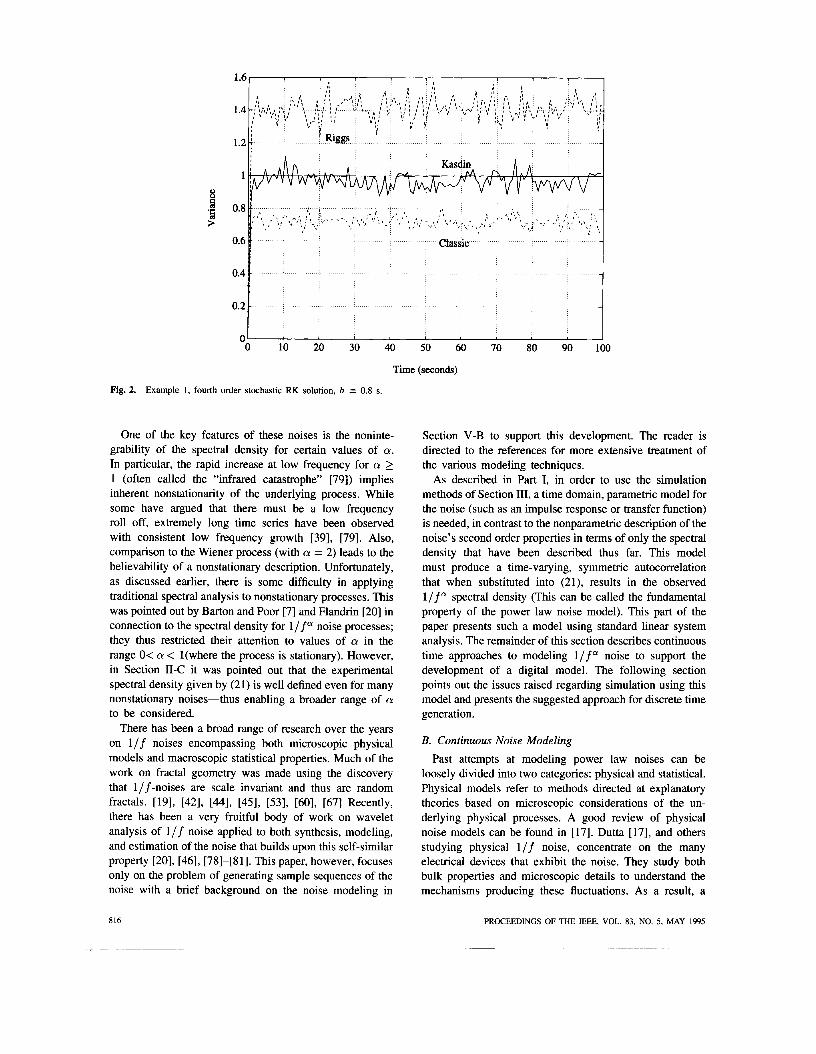
Fig. 2 plots the true covariance from (82) with the covariance found from averaging 800 sample sequences from three different methods-the RK solution described here, the classical approach using a zero-order hold on the noise, and the RK approach of Eggs described in [58]. More examples of the RK solution technique can be found in [36].

Again, it is conjectured that this same set of coefficients can be used to simulate nonlinear stochastic differential equations as well. Since the derivation was made ignoring the bilinear term, it is believed this extension only works on nonlinear systems that, when linearized for small states, do not have a bilinear dependence on X ( t ) . There is an example in [36] to show the performance on nonlinear systems and current research is examining further examples.

PART 11: l/f" NOISE GENERATION

v. INTRODUCTION TO POWER LAW NOISE MODELING

A. Background In this part I address the specific problem of generating

sequences of power law, or l/f", noise^.^ The name derives from the functional form of the experimentally determined sample spectral density functions (21)-these noises have spectra which grow with low frequency as l/f", where f is the cyclic frequency and a is a real number, usually between 0 and 2.

The l/f" property of some noises (i.e., long term correlation or "infinite memory") has been observed over the years in a myriad of devices and systems. In physics and engineering, it arises in resistance and thermal fluctuations, voltages across vacuum tubes and diodes, and almost every solid state device, frequency fluctuations in oscillators, and voltages in most superconducting devices. This noise has also been observed in such diverse fields as economics (e.g., the Dow Jones Average [79]), music, weather, traffic, and hydrology. The earliest work outside of electrical devices was in studying the rate of rainfall in various locations, which was seen to exhibit a l / f type spectrum. This hydrological work later led to Mandelbrot's development of fractal geometry. Mandelbrot observed that variations, on any scale, in the geometry of natural phenomena (leaves, branches, coastlines, mountains, etc.) also exhibit this l / fa variation in the frequency domain. A rich variety of information on l / f noise studies can be found in [4], 171, 1171, [201, [211, 1381, [391, E421, [571, 1661, 1671, [791.

4These noises are sometimes also referred to as pink noise, flicker noise, burst noise, low frequency divergent noise, and fractional noise.


-0 10 20 30 40 50 60 70 80 90 100

Time (seconds)

Fig. 2. Example 1 , fourth order stochastic RK solution, h = 0.8 s.

One of the key features of these noises is the nonintegrability of the spectral density for certain values of a. In particular, the rapid increase at low frequency for a 2 1 (often called the “infrared catastrophe” [79]) implies inherent nonstationarity of the underlying process. While some have argued that there must be a low frequency roll off, extremely long time series have been observed with consistent low frequency growth [39], [79]. Also, comparison to the Wiener process (with a = 2) leads to the believability of a nonstationary description. Unfortunately, as discussed earlier, there is some difficulty in applying traditional spectral analysis to nonstationary processes. This was pointed out by Barton and Poor [7] and Flandrin [20] in connection to the spectral density for l / fQ noise processes; they thus restricted their attention to values of a in the range O< a < l(where the process is stationary). However, in Section 11-C it was pointed out that the experimental spectral density given by (21) is well defined even for many nonstationary noises-thus enabling a broader range of a to be considered.

There has been a broad range of research over the years on 1 / f noises encompassing both microscopic physical models and macroscopic statistical properties. Much of the work on fractal geometry was made using the discovery that l/f-noises are scale invariant and thus are random fractals. [19], [42], 1441, [45], [53], [60], [67] Recently, there has been a very fruitful body of work on wavelet analysis of l/f noise applied to both synthesis, modeling, and estimation of the noise that builds upon this self-similar property [20], [46], [78]-[81]. This paper, however, focuses only on the problem of generating sample sequences of the noise with a brief background on the noise modeling in

816

Section V-B to support this development. The reader is directed to the references for more extensive treatment of the various modeling techniques.

As described in Part I, in order to use the simulation methods of Section 111, a time domain, parametric model for the noise (such as an impulse response or transfer function) is needed, in contrast to the nonparametric description of the noise’s second order properties in terms of only the spectral density that have been described thus far. This model must produce a time-varying, symmetric autocorrelation that when substituted into (21), results in the observed l / fa spectral density (This can be called the fundamental property of the power law noise model). This part of the paper presents such a model using standard linear system analysis. The remainder of this section describes continuous time approaches to modeling l / f” noise to support the development of a digital model. The following section points out the issues raised regarding simulation using this model and presents the suggested approach for discrete time generation.

B. Continuous Noise Modeling Past attempts at modeling power law noises can be

loosely divided into two categories: physical and statistical. Physical models refer to methods directed at explanatory theories based on microscopic considerations of the underlying physical processes. A good review of physical noise models can be found in [17]. Dutta [17], and others studying physical l/f noise, concentrate on the many electrical devices that exhibit the noise. They study both bulk properties and microscopic details to understand the mechanisms producing these fluctuations. As a result, a


wide variety of equations have been put forth to describe the noise production process. As Dutta explains, however, “the most general models are poorly correlated with experience, whereas the most successful theories are the ones with the most specific applications” [ 171. In other words, each theory is specific to the device being considered, often under certain simplifying approximations.

Statistical modeling refers to a more phenomenological approach. This method is best exemplified by the work of Barnes and Allan [4], Mandelbrot [42], [44], Voss [66], [67], Feder [19], Barton and Poor [7], Flandrin [20], [211, and Wornell [78]-[80]. The approach does not look at the detailed event space of each device or system, but views the phenomenon itself as universal, independent of the specific generating mechanisms. A simple, statistical model is then pursued that can produce the observed (or assumed) properties of the phenomena. Gray [26] calls the probability space associated with the statistical model a “canonical description of the random variable.”

There have been a number of general approaches to modeling 1/ f -noises over the years. The most common fall into three categories-ARMA based models, fractional integration, and wavelet analysis. The earliest approaches to modeling assume an ARMA form for the system generating the noise that fits, in some sense, the 1 / f a spectral form. In other words, they approximate a 1 / sa l2 transfer function by a finite number of time-invariant, linear systems. The most common approximation is to fit this transfer function by a sum of first order Gauss-Markov processes (also called a “superposition of Lorentzian spectra” [791) [4]-[61, [17], [38], [39], [54], [57], [59]. (An equivalent model is the truncated RC line with white noise at its input that uses alternating poles and zeros [271, [381, [391, [791.) By properly choosing the process pole locations and their number, the l / ~ ” / ~ transfer function can be fit to arbitrary accuracy. Mathematically, this approach can be expressed:

There are three problems with this model. The first is its inherent coarseness in describing the spectrum. An infinite number of poles are necessary to exactly reproduce the l / f ” form, and, since any digital mapping must consist of a finite number of poles, errors are incurred when developing a generation technique (though admittedly very small). Mandelbrot refers to this as the “distributed relaxation times panacea” [42].

The second problem with the Gauss-Markov method arises when trying to model the low frequency divergent behavior. As longer sequences are generated, additional poles must continually be added, quickly resulting in an unwieldy model. If the number of poles is truncated, the frequency spectrum will become constant below some limiting frequency, resulting in a stationary process and incorrect spectral density.

Finally, the model is not scale-invariant. The pole locations are inherently functions of time-scale. More is said about scale invariance below.

As mentioned, there has been much work recently on wavelet based models of l/f-noise [78]. As in the Gauss-Markov approach, these models have the property that they can be made to fit the spectrum with arbitrary accuracy. In other words, by selecting the proper basis, the proper coefficients, and using a large enough set of terms in the wavelet expansion, the spectral density of the wavelet based process satisfies [781:

k l k2 - < S ( W ) 5 -. 14” - IWI“ (84)

This property is identical that of the ARMA based models above. In addition, the wavelet approach has the advantage of preserving the scale invariance of the modeled process (since wavelets are a time-frequency expansion they are naturally invariant to dilations and translations of the time axis). Unfortunately, for any finite number of terms, the resulting spectrum still has ripple about the l/f form [78]-[80]. It is also more challenging to relate the wavelet based model to a more physical systems approach for generation as in Part I.

In the remainder of this paper I use the third statistical approach to modeling due to Mandelbrot and Van Ness [45]. As pointed out by Wornell [78], this can be viewed as further development of the work of Barnes and Allan [4]. This model is developed by observing the obvious simil-ty between 1 / f“ noise and Brownian motion, where S 0; l / f ” Mandelbrot generalized this concept by introducing his definition of fractional Brownian motion (FBM). In this case, the Wiener process is simply a special case of the FBM for a = 2. Fractional Brownian motion can thus be defined exactly as Brownian motion in Section 11-B except with a slight modification to property b. The Fractional Brownian motion process, B(t) , is defined as a zero mean stochastic process that satisfies the following

properties:

B(0) = 0.

B(t2) - B(tl), B(t3) - B(t2), ’ . . , B(tn) - B(L-1)

B f ( t ) - B f (s) is stationary and normal with mean 0 and variance C( It - sla-’ for s 5 t.

are independent for tl 5 t 2 5 . . . 5 tn. In addition to this generalization, Mandelbrot

added a fourth property of fractional Brownian motion. He used a variety of experimental and observational evidence to justify his claim that l / f a noise is a fundamental property of nature. As mentioned, his study of power law ubiquity led directly to his development of fractal geometry for describing nature and thus classifying 1 /fa noise as a type of random fractal [191, [421, [441, [451, [53], [601, [67]. This description produces the fourth property of the FBM model: The FBM B f ( t ) is self-similar (or scale invariant and thus is a random fractal).


Scale invariance refers to the independence of the model from the scale of observation. The fact that l/f noises (and Brownian motion) are scale invariant is suggested by their autospectral densities. If the frequency scale is changed, the original amplitude scaling can be obtained by simply multiplying by an appropriate constant. It was Mandelbrot's observation of the universality of scale invariance that led to this elevation as a fundamental property. In fact, it can be argued that it is this property that is universal and accounts for the proliferation of power law noises throughout nature.

To be more precise, the l/f" random process is self- affine. Feder [19] defines a self-affine random process by the scale-invariance of its time-varying probability density function:

[19] where the new time scale, 5, has been scaled from the old one by the factor b. Note that a self-similar (rather than self-affine) process is one where the power, H, is unity.

Here, this definition is referred to as strictly self-affine. As in the stationarity and simulation definitions, the self- affine property can be made more general by defining a wide-sense self-affine process as one where only the first and second order moments are scale-invariant. That is, the autocorrelation function has the property:

R(bt, bT) = b - H R ( t , T ) . (86)

In the sequel, we only require that the noise models satisfy (86). However, for Gaussian noise processes (such as those considered here), wide sense scale-invariance is equivalent to strict scale-invariance.

C. Fractional Brownian Motion Unlike for standard Brownian motion (a = 2), it is

difficult to derive from the above definition an unambiguous autocorrelation function that can lead to a generation model for l / f a noises. Instead, Mandelbrot [40]-[45] used the approach of Barnes and Allan [4] and suggested extending this Wiener process generalization to the Laplace domain by assuming a transfer function of the form l/sa/', and then invoking the fractional calculus. Thus just as white noise is the derivative of Brownian motion, we define l/fa noise via the fractional derivative:

where a is a real number, normally between 0 and 2. There a many texts on the fractional calculus [16], [49], [50] and it is beyond the scope of this paper to discuss the existence details of (87). It can be shown, however, that the anti-derivative corresponding to (87) is given by the Riemann-Liouville fractional integral [50] :

z ( t ) = - f ( t - T)"/"-'w(r) d r . (88) r(Q/2) 0

This is equivalent to a linear system driven by white noise with impulse response function:

whose Laplace transform is l/s"/' as desired [18]. As we'll see, this definition of FBM has some problems.

For Q < 1 it is difficult to define h(t) at t = 0 (this results in the lack of a well defined variance). The model also does not, in general, produce stationary and independent increments satisfying property 2) above. Mandelbrot, and later Barton and Poor and Flandrin, tried to correct this problem by modifying the fractional Brownian motion integral as follows:

This definition, however, does not solve the problem for noise generation as it does not represent a causal, time- invariant linear system (there is no well defined impulse response function). Instead, I will use in this section the traditional definition proposed by Barnes and Allan [4] in (88). It will be shown that asymptotically the model possesses the desired properties. The problem at t = 0 will be corrected in Section VI when a digital model for generation is introduced.

Note that many of these problems have been recognized before. This is particularly true in the cases where the fractional integration model in (90) is used as a definition of l / f noise. In fact, Wornell [79] avoids them by proposing a different, frequency based definition for the l/f process and shows that Fractional Brownian Motion satisfies that definition as well as his wavelet based model to some desired accuracy. However, the value of a time based definition was explained in Part I, particularly regarding the development of correlation properties to be used in developing generation models. It is believed that the fractional Brownian motion definition given above is the most general and provides the most direct connection to the Wiener process. The fractional integration equations are shown to satisfy this definition in some limits. The fact that they do not satisfy the definition in all cases does point out problems with the model, but they provide a convenient avenue to developing the discrete model in Section VI that is used to generate l/f-noises and that does satisfy all the desired properties of a FBM.

Given the convolution integral and impulse response function in (88) and (89), the autocorrelation function can be computed using (27). These integrals, however, must be solved separately for Q = 1 and cy not equal to 1. These cases can all be solved via integrals in [25]. For Q = 1, this becomes


and, for a # 1:

where zFl(a, /3; y; z ) is the hypergeometric function. As mentioned, it is impossible in general to use (92)

to show that the process has independent and stationary increments satisfying condition b. It is also impossible to use (92) in (21) to produce the desired l/f" form of S. We therefore examine the asymptotic autocorrelations for t >> r:

(93) Q R(t,T) E -(log 4t - log 1.1) 27r

for a = 1, and

R(t, r ) Z Q { r(l - a);in(7ra/2) Jrla-'

(94)

for a # 1. Thus for a < 1 , the process is stationary-the time

dependence in (94) goes to zero for large t. However, the variance is undefined as T approaches zero (and as t gets small). This problem has been called the "high frequency (or ultraviolet) catastrophe" [39], [42], [79] and results from the nonintegrability of the spectral density at high frequency as well as low frequency for a < 1. The high frequency problem has manifested itself for Q: < 1 in two ways-the inability to determine h(t) for t = 0 and the nonexistence of a well defined variance.

For a > 1, the autocorrelation in (94) shows that, like Brownian motion, the process is nonstationary. Though it has been claimed that eventually the power must flatten at low frequency (possibly due to a second process taking over), for many values of a the growth is so slow that, on the observation time scales of interest, nonstationary behavior cannot be ruled out (see also [38], [39]). In fact, such a low frequency cutoff has never been observed experimentally, despite extensive attempts at obtaining very long time sequences.

This asymptotic expansion of the autocorrelation for large t can be substituted into (21) to show that the measured spectral density of a sample sequence for large time does result in the desired form (l/w"), proving that the model asymptotically satisfies the fundamental property. In addition, these autocorrelation functions are self-affine, satisfying property d. Finally these autocorrelation functions can be used to show that the model results, asymptotically, in stationary increments with the form required by property b. For a > 1 and large t , the variance of the increments is

lAtl"-' (95) 2r(2 - a) sin(7ra/2)

7r(a - 1) ff; r

where 0; is equal to E{IBf ( t ) - Bf(s ) l } and At = t - s.

Unfortunately, for a < 1, it is impossible to show that the increment property is satisfied because of the high frequency difficulties (that is, an undefined variance). There- fore, in the next section a new discrete model is proposed that, among other advantages, alleviates this high frequency problem.

VI. DISCRETE GENERATION METHOD In this section methods are discussed for simulating 1 /fa

power law noises. In Section VI-A the past techniques are reviewed with an arrow toward some of their difficulties. Then, in Section VI-B, a new method is presented to generate power law noise that satisfies the requirements of the fractional Brownian motion definition. This is done by postulating a pulse response function that can be used in (37) and can be shown to satisfy the definition of an accurate simulation-that is, of sampling the autocomlation function. Lastly, in Section VI-E, this approach is simplified with two approximate techniques for generating power law noise that result in the desired spectral density only over a finite frequency range.

A. Past Methods A difficulty arises in trying to simulate 1 /fa noises using

the methods of Section I11 because there is no well defined set of differential equations (or rational transfer functions) that can be used for time domain modeling. Most past work on simulation, therefore, has focused on methods that approximate the l/f" spectrum to some level of accuracy. In fact, Voss [67], Feder [19], and Peitgen [53] produce l/f" sequences by generating random spectra directly as described in Section 111-A (this technique is frequently used for generating fractal landscapes in two and three dimensions). The difficulties associated with this method have already been described.

A number of researchers have attempted time domain simulation using the fractional integration model given by (88) or (90). In particular, they use the technique described in Section 111-B and replace the convolution integral in (88) with a convolution sum. They determine the pulse response by simply sampling the impulse response function given in (89). Examples of this approach can be found in [191, [531, [401, 1411.

Section I11 has already described the errors in this generating method when h(t) is not found from a rational transfer function. In addition to these errors, there is the high frequency problem-for a < 2, h(0) = CO. How, then, does one select h(O)? Most often, this ambiguity is avoided by using a value of either 0 or 1 [57]. Radeka [57] argues that physically there must be some high frequency cutoff and therefore a limit on h(t) before some time S is reasonable. Unfortunately, this problem is deeper than the mere technical difficulty of sampling h(t). As described earlier, the autocorrelation function shows a fundamental error at high frequency inherent in the model of (88).

KASDIN DISCRETE SIMULATION OF COLORED NOISE AND STOCHASTIC PROCESSES

~ -~ _ _ __

819

Most other time domain approaches use the approximate models described in Section V-B (Gauss-Markov (ARMA) fits) and then apply the methods of Section I11 for generation. In fact, Barnes finds the coefficients of the discrete, linear filter directly by ARMA identification techniques on noise sequences. While the generation techniques for such models are well established, the problems with the models themselves have already been discussed.

The next section presents an alternative approach first proposed by Hosking [31] to digital simulation that avoids these problems and produces a noise sequence with all the desired properties. Its attractiveness lies in its direct relationship to the Laplace transform model of Fractional Brownian Motion and its satisfaction of the FBM definition. It is hoped that by studying some of the limit properties of the model, more can be learned about the difficulties in the continuous FBM model of Section V-C.

B. Digital Noise Model As shown in Section 111-E, it is straightforward to find a

discrete simulation model for the Wiener process (a = 2). This was given in (64):

1 H(z) = ~ 1 - z-l ' z > l .

This corresponds to a pulse response equal to the unit step (in this special case, equivalent to samples of the continuous impulse response). Again, with this pulse response, the method of Section 111-B can be used to generate the noise.

As mentioned in Section IT-B, this discrete model for the Wiener process is often used in an alternative derivation of Brownian motion that removes some of the theoretical difficulties in defining white noise. That is, Brownian motion is defined by the limit of the discrete random walk as At + 0. Papoulis [52] has an excellent derivation where he shows that all of the properties in Section 11-B follow from this limiting procedure. Since the random walk describes a process of independent random increments at each step, the limiting definition has the intuitive advantage that it follows from our physical understanding of the process.

This leads to the conjecture for a discrete power law noise model. Just as the continuous fractional Brownian motion model described in Sections V-B and V-C was proposed as a generalization of the continuous Wiener process using fractional integration, a generalization of the random walk of (96) is proposed as the digital model:

z > l . (97)

This model was independently put forth by Hosking [31] and called fractional differen~ing.~ The conjecture is that

SHosking used a statistical, time series analysis approach in his definition. He therefore used the backward difference operator to define fractional differencing via:

an improved continuous model for power law noise can be derived as the limit of (97) for small time.

This model resolves all of the difficulties with other generation methods. The problems with discrete modeling of a pure 1 / ~ " / ~ filter are solved because the windowing and Nyquist frequency issues are implicitly part of the model in (97). As we'll see, the high frequency problems are solved because the transfer function in (97) results in a well defined pulse response for all times. The process defined by (97) is nonstationaxy (for a 2 1) and self- affine-there is no explicit time step in (97). The discrete transfer function in (97) is the same for all time steps-as At is varied, only the amplitude changes. This scale- invariance is made clear by examining the spectral density associated with (97). As described in Part I, the discrete spectral density is found via s d = A@dH(z)H(z-l) with

r91: = @At

where Qd is the variance of the IID input noise process.

well approximated by For frequencies below the Nyquist frequency, this can be

(99)

As described in Section 111-F, the distortion near the Nyquist frequency in (98) is due to sampling and aliasing-that is, the model in (98) implicitly assumes a l/f" process that has been sampled without prefiltering. It is very difficult to build into the simulation process discussed below the effects of prefilters to reduce the distortion near Nyquist. However, as discussed in Section VI-E, normally this noise is summed with high frequency white noise (generated by the approximation described in Section 111-F) that dominates the portion of the spectra near Nyquist. Thus the small distortion in the spectral density due to aliasing is usually unimportant.

This model produces an experimental spectral density proportional to l/f" as seen in (99). Equation (99) clearly points out the self-affine nature of the model. In fact, it also indicates the method for choosing Qd. Since a simulated process is desired with spectral density Q/(27rf)", (99) shows that Qd should be chosen via:

The digital pulse response associated with the model in (97) is found by the power series expansion of the transfer function:

This results in a pulse response, by the definition of the z-transform, as the coefficients of this series. That is

k

h k = - n=l

k! for real, noninteger d.


where (a/2)k is known as Pochhammer's symbol [l] and is a notation for the geometric series given by the kth numerator in (101) or, equivalently, the lcth derivative of 1/(1 - x ) ~ / ' evaluated at x = 0. Using [ l ] this is equal to

These pulse response values can be easily computed using the following recursive algorithm:

ho 1

Again, the discrete model has solved the high frequency problem-hk is well defined and equal to one at zero for all values of a.

An expression for the increment process of FBM can be found using this model and the pulse response given above. Expressing the first differences of the process as AXk = x k + l - Xk:

This is an asymptotically stationary process with variance (in the limit of large k):

00

1 + (; - 1)' A} (m + 1) (106) m=O

where u2\ is the discrete variance of the increment equivalent to 0: in (95).

Thus the increment process has the correct dependence upon time (Ata-l) as required by the definition. It also results in a defined variance for 0 < a < 1, unlike the continuous model. Note that the expression in (106) converges very fast. For a = 1, it reaches a relative accuracy of 5 x lo6 in 25 steps.

Finally, we can use (38) to find the discrete autocorrelation function associated with the noise. In general, there is no closed form solution for Rd(k,m) as the noise is nonstationary. However, for (Y < 1, the process is stationary and the autocorrelation can be examined in the large t limit as in Section V for the continuous model.6 Hosking [31] shows this using the inverse Fourier transform on (98). An alternative approach in the time domain uses (38) to find:

6Hosking [31] points out that for values of a > 1 the process can be considered as equivalent to the integration of the stationary process with power law behavior f'-". This argument must be used with care, however. A straightforward application to the steady state system would compute a linearly increasing variance-learly incorrect from (5.16). The error is in neglecting the transient in the variance for a < 1 that decreases as l/t". When multiplied by the random walk the transient does not decay but increases as t l p U .

Or, upon solving the sum:

Using [l], the definition of Pochhammer's symbol, and fundamental properties of the gamma function this can be simplified to

where, as stated earlier, Qd = QatQ-', so the self- similar property holds. This can be further simplified, using fundamental properties of the gamma function, or found directly using the frequency domain approach [31], to be

As mentioned earlier, (84) shows that the variance is undefined for the continuous, fractional integration form and (Y < 1-indicating an underlying difficulty with the model. The discrete model proposed here results in a well defined and computable variance for values of a < 1. Setting m = 0 in (108):

Finally, it was claimed earlier that the discrete model in (97) produces an improved continuous llf" noise model in the limit as At -+ 0. One consistency check is to examine the autocorrelation function, for a < 1, in (109) in this limit and compare to the continuous model autocorrelation function for large T (94). This can be done by multiplying and dividing (109) by At"-', letting At -+ 0 while keeping Qd/At"-' = Q constant, letting mat -+ r, and using the formula:

2b-a r (Z + r ( z + b)

( a - b) (a + b - 1) 22 -+ 1 +

2'00

1 + ; ( a b ) ( 3 ( . + b - 1)' - a + b - 1)- 22 + . . .

from [I]. This results in the following formula for the continuous autocorrelation in the limit as At -+ 0 and for large lag (m or 7):

Qr(1- a ) sin(m/2) 7.r

R L ( T ) =

KASDIN: DISCRETE SIMULATION OF COLORED NOISE AND STOCHASTIC PROCESSES

____ ~~

82 1

Simulated I/f Noise Smuence 4 , 1

-4-

-5 200 400 600 800 lo00 1200

TUIE

Fig. 3. Example of generated l/f noise sequence.

Thus for large T or At + 0, the autocorrelation of the digital model in the limit is identical to that for the continuous one in (94). Note that we have used the notation here RL(T) to distinguish this autocorrelation in the limit from that in (94). This is a very satisfying result, particularly when compared to the derivation of Brownian motion as the same limit of the discrete random walk (a = 2). It also confirms (97) as an adequate simulation model as it satisfies Definition 1-it samples the autocorrelation of the continuous process. Future work is directed at deriving a general expression for Rd(k,m) for all a and thus show that the complete nonstationary autocorrelation in (94) for all T can be derived via this limit of the discrete model.

In addition to the autocorrelation and spectral density correspondences examined above, noise simulated by this method has been examined using the Allan variance [35], [68], [69]. It was confirmed that for time lags large compared to the sampling time the Allan variance converged to that expected for power law models.

C. MA and AR Generation Methods Finally, I address the specific implementation question

for generating sequences of noise from the discrete model discussed above. Just as continuous llf" noise models have no finite set of differential equations to describe them, the discrete model in (97) has no finite set of difference equations that can be used for generation (as in Section 111-D). However, there are two equivalent methods that can be used to generate finite length noise sequences-FIR and IIR filtering.

The finite impulse response (FIR) or moving average (MA) method for noise generation uses (104) directly for generating noise. That is, the method of Section 111-B is used with the pulse response values given by (104). Thus the noise can be generated either by direct convolution or by multiplication in the frequency domain. Appendix 11 lists a

C computer program for this frequency domain generation of llf" noise.

The main drawback of this technique is its memory burden. Because it is a batch method, it can require large amounts of memory for long time sequences. In addition, only sequences whose length are powers of 2 with standard Cooley-Tukey FFT routines can be generated in short times [5 11. Section VI-E describes two approximate methods for generating noise that requires less memory and time with minimal spectral distortion.

A second technique is analogous to infinite impulse response (IIR) filtering or autoregressive (AR) time series. Here, only the denominator of the transfer function in (97) is expanded:

. (114) 1 H ( z ) =

2

. (114) 1 H ( z ) =

2

This transfer function is equivalent to a recursive (AR) filter:

The filter coefficients can be easily found from an itera- tive formula similar to that for the MA case:

a0 = 1

This AR formula can be used for time domain sequence generation as an alternative to the MA, frequency domain method. It requires significantly less memory and does not restrict sequence lengths to a power of two-only previous values of the sequence itself need be stored. It is also well suited to real time generation. Unfortunately, it is significantly slower than the frequency domain methods. At each new step, a new coefficient must be computed and included in the filter with the size of the filter growing with time.

Though it was stated that there are no sets of difference equations that can reproduce the model in (97), the AR filter in (115) does not present a contradiction. This is indeed a difference equation, but it cannot be reproduced by a finite set of first order equations. For each new time there is a new a,. In other words, an infinite number of initial conditions are required (or, alternatively, the filter has an infinite number of poles). This is a reflection of the infinite memory or long correlation time property discussed in Section I1 [7], [17], [31], [38], [39], 1421, [43], [45]. The AR form in (1 15) provides an alternative interpretation of the infinite memory property than that represented by the slow decay of the autocorrelation.

D. Example Fig. 3 presents a simulated llf" noise sequence with a =

1 using the exact FIR generation method. An example computer program for the procedure is listed in Appendix 11.


Spectral Density of Simulated l/f Noise Sequences

Frequency (Hz)

Fig. 4. Autospectral density of generated l/f sequence.

Fig. 3 is the computed spectral density of the sequence. The dashed line is the exact spectral density from (98).

E. Approximate Generation Methods Lastly, it is useful to consider possible approximate

methods for generation. In these techniques, certain of the required properties are violated in favor of faster or more efficient generating algorithms. In particular, the noise has a llf" spectral density only over a finite range of frequencies-much as in the Gauss-Markov or ARMA generating method. However, unlike previous methods, the processes produced here remain self-affine. It should be noted that the wavelet based approximate models in [78]-[80] also provide very efficient means for generating sequences of noise. In addition, a good deal of work has been done (and continues) on the analysis and synthesis of llf noise using the wavelet model, particularly regarding estimation of signals and noise and signal processing. While this is an important problem, it is beyond the scope of this paper to discuss in any detail. The reader is directed to [79] and [80] for summaries of this work.

1) Truncation Method: The first technique involves truncation of the series of coefficients in (104) or (113). If a finite set of pulse response values is used, then the generating algorithm involves FIR filtering of the input noise. Alternatively, the series in (1 13) can be truncated to produce a finite length difference equation or IIR filter. In both cases, the spectrum has a l lf" form down to a

limiting frequency related to llNAt, where N is the length of the truncated coefficient series. Below this frequency the spectral density is flat-the noise is stationary for all a. This approximation is useful when only the high frequency llf" behavior is important. The FIR implementation is faster but with more distortions to the spectrum within the band of interest (due to windowing errors) than the IIR filter. In general, an IIR implementation is recommended. Fig. 5 shows the spectral density for a llf (a = 1) IIR filter (dashed), FIR filter with rectangular window (solid), and FIR filter with Kaiser window, /3 = 4 (dotted). Also shown is the exact l/f line (dot-dashed). Note that each of these approaches is self-affine-time enters only as an amplitude scaling.

2) Filtering Method: The main drawback to the truncation method is that the resulting sequence is stationary. In many applications, however, it is of great interest to observe the effects of the growing noise variance with time. Of less interest is the very high frequency (behavior above some limiting frequency). Normally, the apparatus being modeled has a white noise component which, when added to the power law noise, dominates the spectrum above this frequency. Thus the l lf" noise can be simulated using the techniques of Section VI-C at a slower rate determined by the high frequency limit of interest (At,). These noise values are held constant over the total interval covered by the faster simulation step (At = At,/n). The resulting sequence is processed with a high order low pass filter whose cutoff is at llAt,. The result is a noise process with

KASDIN: DISCRETE SIMULATION OF COLORED NOISE AND STOCHASTIC PROCESSES

~- - ~~ __

823

103

102

.L( E 5 101 n 2 8 3 9 100 4

U2

Fig. 5. Autospectral densities for truncation filters.

1/ f O1 behavior from zero to llAt, Hz and negligible power at higher frequencies. White noise can then be added at the appropriate magnitude to complete the simulation.

VII. CONCLUSIONS This paper was intended to serve two purposes. First, it

was meant as a tutorial and broad review on noise generation. Thus Part I presented a review of basic stochastic processes and linear systems applied to noise simulation. At the same time, this part presented a number of new results in spectral density computation, Brownian motion, and discrete stochastic processes. It critiqued some past methods for noise generation (particularly frequency domain techniques based on spectral density fitting) and presented a new definition for noise simulation. It presented a systematic approach to digital noise modeling and generation based on standard continuous and discrete linear system theory. It also presented a summary [36] of a new RK simulation technique for stochastic differential equations.

The second goal of this paper was to present an overview of past work on modeling of llf" power law noises and to use the methods of Part I for simulating these noises. Past llf noise generation techniques were reviewed and critiqued. The model first proposed by Hosking 1311, and independently by the author, was proposed not only as an effective means of generating the noise but also as an approach for continuous modeling in the limit that corrects some of the theoretical difficulties with past approaches. Two generation algorithms were presented based upon this

824

model and the techniques of Part I with sample code listed in the appendix. Some approximate techniques that require less memory and are more efficient were also discussed. The result is an efficient and accurate algorithm that can be easily implemented for simulating power law noises.

APPENDIX I VAN LOEN ALGORITHM

The Van Loen algorithm is a numerical technique developed by C. F. Van Loen [65] for solving the quadratic integral in (54). The solution is found by forming the matrix exponential:

[: z] =exp(CAt)

where C is a block upper triangular matrix:

There are numerous techniques for computing the matrix exponential [48]. The most straightforward is to find the eigenvalue decomposition and take the exponential of each eigenvalue.

The solution to the integral in (54), Q d , is then given by the matrix equation:

PROCEEDINGS OF THE IEEE, VOL. 83, NO. 5 , MAY 1995

void f-alpha(int n-pts, float X[],float Q-d, float alpha, int *idum)

int i,nn; float *hfa,*wfa; float ha,wr,wi; nn = n-pts+npts; ha= alpha/2.0 ; Q-d=sqrt (Q-d) ; / * find the deviation of the

hfa=vector(l,nn); wfa=vector(l,nn); hfa[ll=l.O; wfa [ 1 I =Q-d*gas-dev ( idum) ; for (i=2 ; i<=n-pts; i++) {

{

noise * /

/ * generate the coefficients hk * / hfa [il =hfa [i-ll* (ha+ (float)

(i-2) / ( (float) (i-1) ) ; / * fill the sequence wk with white noise * /

wfa [i] =Q-d*gas-dev (idum) ; 1

/ * pad the ends of the sequences with zeroes * / for(i=n-pts+I;i<=nn;i++) {

hfa[i] =O. 0; wfa [i] = O . 0;

1 / * perform the discrete Fourier transform * / realft (hfa,npts, 1) ; realft (wfa,n-pts, 1) ;

wfa[ll=wfa[ll *hfa[ll ; wfa [2 I =wfa [2 I *hfa [ 2 3 ; for(i=3;i<=nn;i+=2){

wr=wfa[i]; wi=wfa [i+l] ; wfa[il=wr*hfa[il-wi*hfa[i+ll ; wfa[i+l]=wr*hfa[i+ll+wi*hfa[i] ;

/ * multiply the two complex vectors * /

1 / * inverse Fourier transform the result * / realft (wfa,n-pts, -1) ; for (i=l; i<=n-pts; i++)

/ * add the final result to X[]*/ X[il+=wfa[i]/( (f1oat)n-pts);

free-vector (hfa, 1,nn) ; free-vector(wfa, 1,nn) ;

1

APPENDIX I1 l/f" NOISE GENERATION CODE

ACKNOWLEDGMENT The author would like to express his gratitude to Dr.

Todd Walter for his invaluable help and contributions to

the simulation program.

The is a program for generating a sequence this manuscript and for providing the C Code version of of llf" noise using the frequency domain, multiplication method (FIR technique) [35]. The routine is coded in C and makes use of algorithms from Numerical Recipes in C [56] (namely gas-dev( ) for Gaussian random number generation and ( for the discrete Fourier See the algorithm shown at the top of this page.

REFERENCES [ 11 M. Abramowitz and I. A. Stegun, Handbook of Mathematical

Functions. New York Dover. 1972.


[2] A. Ambrcjzy and L. B. Kiss, “llf noise generator,” in Proc. 8th Int. Con$ on Noise in Phys. Syst. and the 4th Int. Con$ on ‘1/ f Noise’, A. Diamico and P. Mazzetti, Eds., Rome, Sept. 1985. Amsterdam: North Holland, 1986, p. 445.

[3] F. T. Arecchi, R. Badii, and A. Politi, “l/ f spectra in nonlinear systems with many attractors,” Noise in Physical Systems and l/f Noise, M. Savelli, G. Lecoy, and J.-P. Nougier, Eds., Proc. 7th Int. Con$ on Noise in Phys. Syst. and the 3rd Int. Con$ on ‘ 1 8 Noise’, Montpellier, May 1983. Amsterdam: North Holland, 1983.

[4] J. A. Barnes and D. W. Allan, “A statistical model of flicker noise,” Proc. IEEE, vol. PROC-54, p. 176, Feb. 1966.

[5] J. A. Barnes and S. Jarvis, “Efficient numerical and analog modeling of flicker noise processes,” Tech. Note 604, Nat. Bur. Stands., 1971.

[6] J. A. Barnes, “Simulation of oscillator noise,” Austron, Inc., Austin, TX.

[7] R. J. Barton and H. V. Poor, “Signal detection in fractional Gaussian noise,” IEEE Trans. In$ Theory, vol. 34, Sept. 1988.

[8] T. H. Bell, Jr., “Representation of random noise by random pulses,” J. Appl. Phys., vol. 45, no. 4, 1974, p. 1902.

[9] J. S. Bendat and A. G. Piersol, Random Data: Analysis and Measurement Procedures.

[lo] K. Y. R. Billah and M. Shinozuka, “Numerical method for colored-noise generation and its application to a bistable system,” Phys. Rev. A, vol. 42, no. 12, pp. 7492-7495, Dec. 1990.

[ 111 R. N. Bracewell, The Fourier Transform and Its Applications. New York McGraw-Hill, 1986.

[12] R. G. Brown and P. Y. C. Hwang, Introduction to Random Signals and Applied Kalman Filtering. New York: Wiley, 1992.

[13] A. E. Bryson and D. E. Johansen, “Linear filtering for time- varying systems using measurements containing colored noise,” IEEE Trans. Auto& Contr., vol. AC-IO, p. 4, 1965.

[14] A. E. Bryson and Y. C. Ho, Applied Optimal Control. New York Hemisphere, 1975.

[15] S. D. Conte and C. de Boor, Elementary Numerical Analysis, An Algorithmic Approach.

[16] A. Dold, A. and B. Eckmann, Fractional Calculus and Its Applications. New York Springer-Verlag, 1975.

[17] P. Dutta, “Low frequency fluctuations in solids: l/f noise,” Revs. Modem Phys., vol. 53, no. 3, p. 497, 1981.

[ 181 A. Erdklyi, Tables of Integral Transforms, vol. 1. New York McGraw-Hill, 1954.

[19] J. Feder, Fractals. New York Plenum, 1988. [20] P. Flandrin, “On the spectrum of fractional Brownian motions,”

IEEE Trans. In$ Theory, vol. 35, Jan. 1989. [21] -, “Wavelet analysis and synthesis of fractional Brownian

motion,” IEEE Trans. In$ Theory, vol. 38, Mar. 1992. [22] G. F. Franklin, J. D. Powell, and A. Emami-Naeini, Feedback

Control of Dynamic Systems. Reading, MA: Addison-Wesley, 1986.

[23] G. F. Franklin, J. D. Powell, and M. L. Workman, Digital Control of Dynamic Systems. Reading, MA: Addison-Wesley, 1990.

[24] J. J. Gagnepain, J. Groslambert, and R. Brendel, “The fractal dimension of phase and frequency noises: Another approach to oscillator characterization,” in Proc. 39th Annu. Freq. Contr. Symp. 1985, 1985, p. 113.

[25] 1. S. Gradshteyn and I. M. Ryzhik, Table of Integrals, Series, and Products. New York Academic, 1965.

[26] R. M. Gray and L. D. Davisson, Random Processes: A Mathematical Approach for Engineers. Englewood Cliffs, NJ: Prentice-Hall, 1986.

[27] P. Gruber, “1/ f -noise generator,” Noise in Physical Systems and 1/ f Noise-1985. A. Diamico and P. Mazzetti, Eds., Proc. 8th Int. Con$ on ‘Noise in Phys. Syst. ’ and the 4th Int. Conf on ‘18 Noise’, Rome, Sept. 1985. Amsterdam: North Holland, 1986, p. 357.

[28] D. Halford, “A general mechanical model for I f ] “ spectral density random noise with special reference to flicker noise

[29] T. Hida, Brownian Motion. New York Springer-Verlag, 1980. [30] P. G. Hoel, S. C. Port, and C. J. Stone, Introduction to Stochastic

[31] J. R. M. Hosking, “Fractional differencing,” Biometrika, vol.

New York Wiley, 1984.

New York McGraw-Hill, 1980.

1/1 f 1,” P ~ o c . IEEE, vol. PROC-56, p. 251, Mar. 1968.

Processes. Boston: Houghton Mifflin, 1972.

68, no. 1, pp. 165-176, 1981.

[32] M. K. Jain, Numerical Methods for Scientific & Engineering Computation. New York: Wiley, 1985.

[33] T. Kailath, Linear Systems. Englewood Cliffs, NJ: Prentice Hall, 1980.

[34] P. Kartaschoff, “Computer simulation of the conventional clock model,” IEEE Trans. Instrum. Meas., vol. IM-28, pp. 193-197, 1979.

[35] N. J. Kasdin and T. Walter, “Discrete simulation of power law noise,” in Proc. 1992 IEEE Frequency Contr. Symp., Hershey, PA, May 1992, pp. 274-283.

[36] N. J. Kasdin, “A Runga-Kutta algorithm for the numerical integration of stochastic differential equations,” to be published in A I M J. Guidance, Control, and Dynamics.

[37] S. M. Kay, “Efficient generation of colored noise,” Proc. IEEE, vol. PROC-69, pp. 480481, 1981.

[38] M. S. Keshner, “Renewal process and diffusion models of l /f noise,” Sc.D. dissertation, Dept. EECS, MIT, 1979.

[39] -, “l/f noise,” Proc. IEEE, vol. PROC-70, p. 211, Mar. 1982.

[40] B. B. Mandelbrot, “A fast fractional Gaussian noise generator,” Water Resources Res., vol. 7, no. 3, June 1971.

[41] B. B. Mandelbrot and J. R. Wallis, “Computer experiments with fractional Gaussian noises. Part 1, averages and variances,” Water Resources Res., vol. 5 , no. 1, Feb. 1969.

[42] B. B. Mandelbrot and R. F. Voss, “Why is nature fractal and when should noises be. scaling?” Noise in Physical Systems and l /f Noise, M. Savelli, G. Lecoy, and J.-P. Nougier, Eds., in Proc. 7th Int. Con$ on ‘Noise in Phys. Syst.’ and the 3rd Int. Con$ on ‘I/fNoise’, Montpellier, May 1983. Amsterdam: North Holland, 1983.

[43] B. B. Mandelbrot, “Some noises with l /f spectrum and a bridge between direct current and white noise,” IEEE Trans. In$ Theory, vol. IT-13, p. 289, Feb. 1967.

[44] -, The Fractal Geometry of Nature. San Francisco: Free- man, 1977.

1451 B. B. Mandelbrot and J. W. Van Ness, “Fractional Brownian motions, fractional noises and applications,” SIAM Rev., vol. 10, no. 4, p. 422, 1968.

[46] W. Martin and P. Flandrin, “Wigner-Ville spectral analysis of nonstationary processes,” IEEE Trans. Acoust., Speech and Signal Process., vol. ASSP-33, Dec. 1985.

[47] N. C. Matalis and J. R. Wallis, “Statistical properties of multi- variate fractional noise processes,” Water Resources Res., vol. 7, no. 6, Dec. 1971.

[48] Matlabm, The Mathworks, Inc., S. Natick, MA, 1992. [49] A. C. McBride and G. F. Roach, Ed., Fractional Calculus.

Boston: Pitman, 1985. [50] K. B. Oldham and J. Spanier, The Fractional Calculus, Theory

and Applications of Differentiation and Integration to Arbitrary Order. New York: Academic, 1974.

[51] A. V. Oppenheim and R. W. Schafer, Discrete-ZIme Signal Processing.

[52] A. Papoulis, Probability, Random Variables, and Stochastic Processes. New York McGraw-Hill, 1984.

[53] H. 0. Peitgen and D. Saupe, Eds., The Science of Fractal Images. New York Springer-Verlag, 1988.

[54] B. Pellegrini, R. Saletti, B. Ner, and P. Terreni, “l/f7 noise generators,” Noise in Physical Systems and 1/ f Noise-1985. A. Diamico and P. Mazzetti, Eds., in Proc. 8th Int. Con$ on ’Noise in Phys. Syst. ’ and the 4th Int. Con$ on ‘IJNoise’, Rome, Sept. 1985. Amsterdam: North Holland, 1986, p. 425.

[55] D. B. Percival, “Characterization of frequency stability: Frequency-domain estimation of stability measures,” Proc. IEEE, vol. 79, June 1991.

[56] W. H. Press, B. P. Flannery, S. A. Teukolsky, and W. T. Vertterling, Numerical Recipes. Cambridge, UK Cambridge Univ. Press, 1986.

[57] V. Radeka, “l/lfl noise in physical measurements,” IEEE Trans. Nuclear Sci., vol. NS-16, p. 17, 1969.

[58] T. L. Riggs, Jr. and C. L. Phillips, “Modeling continuous noise sources in digital simulations,” Simulation, vol. 48, no. 1, Jan. 1987.

[59] R. Saletti, “A comparison between two methods to generate l/ f7 noise,” Proc. lEEE, vol. PROC-74, p. 1595, Nov. 1986.

[60] M. Schroeder, Fractals, Chaos, Power Laws, Minutes from an Infinite Paradise.

[61] T. T. Soong, Random Differential Equations in Science and Engineering. New York Academic, 1973.

Englewood Cliffs, NJ: Prentice Hall, 1989.

New York Freeman, 1991.

826 PROCEEDINGS OF THE IEEE, VOL. 83, NO. 5 , MAY 1995

1621 R. F. Stengel, Stochastic Optimal Control. New York: Wiley, 1986.

[63] V. J. Strasilla and M. J. 0. Strott, “Narrow-band variance noise,” J. Appl. Phys., vol. 45, no. 3, p. 1423, 1974.

[64] C. D. Tesche, “DC SQUIDS with low l/f noise,” Res. Rep., IBM T. J. Watson Res. Center, Yorktown Heights, NY, July 1985.

1651 C. F. Van Loen, “Computing integrals involving the matrix exponential,” IEEE Trans. Autom. Contr., vol. AC-23, Aug. 1978.

[66] R. F. Voss, “Linearity of l/f noise mechanisms,” Phys. Rev. Lett., vol. 40, no. 14, p. 913, 1978.

[67] -, “Random fractals: Characterization and measurement,” Scaling Phenomena in Disordered Systems, R. Pynn and A. Skjeltorp, Eds.

1681 T. Walter, “A multi-variance analysis in the time domain,” in Proc. 24th PTTI Appl. and Planning Meet., McLean, VA, Dec. 1992, pp. 413426.

[69] -, “Characterizing frequency stability: A continuous power law model with discrete sampling,” to be published.

[70] E. Wong and B. Hajek, Stochastic Processes in Engineering Systems. New York Springer-Verlag, 1985.

[71] C. K. Chui, An Introduction to Wavelets. San Diego: Aca- demic, 1992.

1721 A. Laine, Ed., Wavelet Theory and Application. Boston: Kluwer, 1993.

1731 S. K. Srinivasan and R. Vasudevan, Introduction to Random Differential Equations and their Applications. New York: El- sevier, 1971.

[74] P. E. Kloeden and E. Platen, Numerical Solution of Stochastic Differential Equations. Berlin: Springer-Verlag, 1992.

[75] P. E. Kloeden, E. Platen, and H. Schurz, Numerical Solution of SDE Through Computer Experiments. Berlin: Springer- Verlag, 1994.

[76] S. B. Lowen and M. C. Teich, “Power-law shot noise,” IEEE Trans. In$ Theory, vol. 36, Nov. 1990.

[77] M. Grigoriu, “Simulation of diffusion processes,” J. Eng. Me- chanics, vol. 116, no. 7, July 1990.

[78] G. W. Womell, “A Karhunen-Loeve-like expansion for l/f processes via wavelets,” IEEE Trans. Inj Theory, vol. 36, July 1990.

1791 -, “Wavelet-based representations for the l/f family of fractal processes,” Proc. IEEE, vol. 81, Oct. 1993.

New York: Plenum, 1985.

[80] G. W. Womell and A. V. Oppenheim, “Estimation of fractal signals from noisy measurements using wavelets,” IEEE Trans. Signal Process., vol. 40, Mar. 1993.

[81] A. H. Tewfik, “Correlation structure. of the discrete wavelet coefficients of fractional Brownian motion,” IEEE Trans. In$ Theory, vol. 38, pt. 2, Mar. 1992.

[82] L. Lapidus and J. H. Seinfeld, Numerical Solution of Ordinary Differential Equations. New York: Academic, 197 1.

[83] L. Ljung, System Identification, Theory for the User. Engle- wood Cliffs, NJ: Prentice-Hall, 1987.

[84] T. W. Anderson, The Statistical Analysis of Time Series. New York Wiley, 1971.

[85] R. H. Cannon, Dynamics of Physical Systems. New York McGraw-Hill, 1967.

[86] S. B. Lowen and M. C. Teich, “Power law shot noise,” IEEE Trans. In$ Theory, vol. 36, Nov. 1990.

[87] L. Lapidus and J. H. Seinfeld, Numerical Solution of Ordinary Differential Equations. New York Academic, 197 1.

N. Jeremy Kasdin (Member, IEEE) was born in Rochester, NY, on July 1, 1963. He received the B.S.E. degree in mechanical and aerospace engineering and engineering physics from Princeton University in 1985 and the M.S. and Ph.D. degrees in aeronautical and astronautical sci- ences, with a minor in electrical engineering, from Stanford University in 1987 and 1991, respectively.

He is currently the Chief Systems Engineer for the NASA Relativity Mission Satellite (also

known as Gravity Probe B) at Stanford University. From 1991 to 1993, he managed the Phase B studies for the Gravity Probe B spacecraft. His principal research interests are in stochastic process modeling, simulation, optimal estimation, digital control, and satellite attitude control. He is the author or coauthor of over 14 papers in the areas of satellite control, stochastic processes, simulation, and estimation theory.

Dr. Kasdin is a member of Sigma Xi, Tau Beta Pi, and Phi Beta Kappa.

KASDIN. DISCRETE SIMULATION OF COLORED NOISE AND STOCHASTIC PROCESSES

~ ~~ - 827

Date post:	26-May-2018
Category:	Documents
Upload:	nguyentuyen
View:	238 times
Download:	0 times

Discrete simulation of colored noise and stochastic processes … · · 2008-05-25Discrete...

Documents