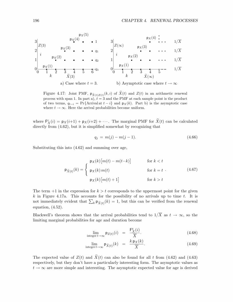
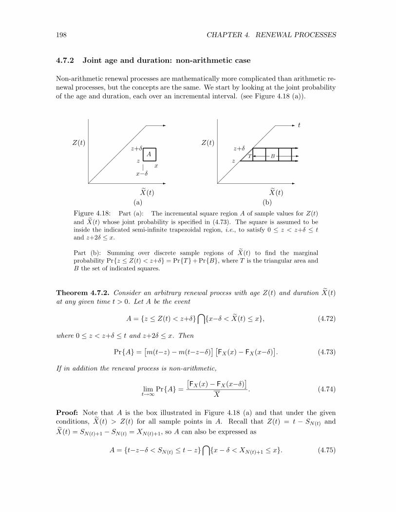
Discrete Stochastic Processes, Chapter 4: Renewal Processes · Chapter 4 RENEWAL PROCESSES 4.1...

Chapter 4

RENEWAL PROCESSES

4.1 Introduction

Recall that a renewal process is an arrival process in which the interarrival intervals are positive,1 independent and identically distributed (IID) random variables (rv’s). Renewal processes (since they are arrival processes) can be specified in three standard ways, first, by the joint distributions of the arrival epochs S1, S2, . . . , second, by the joint distributions of the interarrival times X1,X2, . . . , and third, by the joint distributions of the counting rv’s, N(t) for t > 0. Recall that N(t) represents the number of arrivals to the system in the interval (0, t].

The simplest characterization is through the interarrival times Xi, since they are IID. Each arrival epoch Sn is simply the sum X1 + X2 + + Xn of n IID rv’s. The characterization · · · of greatest interest in this chapter is the renewal counting process, {N(t); t > 0}. Recall from (2.2) and (2.3) that the arrival epochs and the counting rv’s are related in each of the following equivalent ways.

{Sn ≤ t} = {N(t) ≥ n}; {Sn > t} = {N(t) < n}. (4.1)

The reason for calling these processes renewal processes is that the process probabilistically starts over at each arrival epoch, Sn. That is, if the nth arrival occurs at Sn = τ , then, counting from Sn = τ , the jth subsequent arrival epoch is at Sn+j − Sn = Xn+1 + +· · · Xn+j . Thus, given Sn = τ , {N(τ + t) − N(τ); t ≥ 0} is a renewal counting process with IID interarrival intervals of the same distribution as the original renewal process. This interpretation of arrivals as renewals will be discussed in more detail later.

The major reason for studying renewal processes is that many complicated processes have randomly occurring instants at which the system returns to a state probabilistically equiva

1Renewal processes are often defined in a slightly more general way, allowing the interarrival intervals Xi

to include the possibility 1 > Pr{Xi = 0} > 0. All of the theorems in this chapter are valid under this more general assumption, as can be verified by complicating the proofs somewhat. Allowing Pr{Xi = 0} > 0 allows multiple arrivals at the same instant, which makes it necessary to allow N(0) to take on positive values, and appears to inhibit intuition about renewals. Exercise 4.3 shows how to view these more general renewal processes while using the definition here, thus showing that the added generality is not worth much.

156

157 4.1. INTRODUCTION

lent to the starting state. These embedded renewal epochs allow us to separate the long term behavior of the process (which can be studied through renewal theory) from the behavior within each renewal period.

Example 4.1.1 (Visits to a given state for a Markov chain). Suppose a recurrent finite-state Markov chain with transition matrix [P ] starts in state i at time 0. Then on the first return to state i, say at time n, the Markov chain, from time n on, is a probabilistic replica of the chain starting at time 0. That is, the state at time 1 is j with probability Pij , and, given a return to i at time n, the probability of state j at time n + 1 is Pij . In the same way, for any m > 0,

Pr{X1 = j, . . . ,Xm = k | X0 = i} = Pr{Xn+1 = j, . . . ,Xn+m = k | Xn = i} . (4.2)

Each subsequent return to state i at a given time n starts a new probabilistic replica of the Markov chain starting in state i at time 0, . Thus the sequence of entry times to state i can be viewed as the arrival epochs of a renewal process.

This example is important, and will form the key to the analysis of Markov chains with a countably infinite set of states in Chapter 5. At the same time, (4.2) does not quite justify viewing successive returns to state i as a renewal process. The problem is that the time of the first entry to state i after time 0 is a random variable rather than a given time n. This will not be a major problem to sort out, but the resolution will be more insightful after developing some basic properties of renewal processes.

Example 4.1.2 (The G/G/m queue:). The customer arrivals to a G/G/m queue form a renewal counting process, {N(t); t > 0}. Each arriving customer waits in the queue until one of m identical servers is free to serve it. The service time required by each customer is a rv, IID over customers, and independent of arrival times and servers. The system is assumed to be empty for t < 0, and an arrival, viewed as customer number 0, is assumed at time 0. The subsequent interarrival intervals X1,X2, . . . , are IID. Note that N(t) for each t > 0 is the number of arrivals in (0, t], so arrival number 0 at t = 0 is not counted in N(t).2

We define a new counting process, {N r(t); t > 0}, for which the renewal epochs are those particular arrival epochs in the original process {N(t); t > 0} at which an arriving customer sees an empty system (i.e., no customer in queue and none in service).3 We will show in Section 4.5.3 that {N r(t) t > 0} is actually a renewal process, but give an intuitive explanation here. Note that customer 0 arrives at time 0 to an empty system, and given a first subsequent arrival to an empty system, at say epoch S1

r > 0, the subsequent customer interarrival intervals are independent of the arrivals in (0, S1

r) and are identically distributed to those earlier arrivals. The service times after S1

r are also IID from those earlier. Finally, the conditions that cause queueing starting from the arrival to an empty system at t = S1

r

are the same as those starting from the arrival to an empty system at t = 0. 2There is always a certain amount of awkwardness in ‘starting’ a renewal process, and the assumption of

an arrival at time 0 which is not counted in N(t) seems strange, but simplifies the notation. The process is defined in terms of the IID inter-renewal intervals X1, X2, . . . . The first renewal epoch is at S1 = X1, and this is the point at which N(t) changes from 0 to 1.

3Readers who accept without question that {Nr (t) t > 0} is a renewal process should be proud of their probabilistic intuition, but should also question exactly how such a conclusion can be proven.

158 CHAPTER 4. RENEWAL PROCESSES

In most situations, we use the words arrivals and renewals interchangably, but for this type of example, the word arrival is used for the counting process {N(t); t > 0} and the word renewal is used for {N r(t); t > 0}. The reason for being interested in {N r(t); t > 0} is that it allows us to analyze very complicated queues such as this in two stages. First, {N(t); t > 0} lets us analyze the distribution of the inter-renewal intervals Xr ofn {N r(t); t > 0}. Second, the general renewal results developed in this chapter can be applied to the distribution on Xr to understand the overall behavior of the queueing system. n

Throughout our study of renewal processes, we use X and E [X] interchangeably to denote the mean inter-renewal interval, and use σ2 or simply σ2 to denote the variance of the X inter-renewal interval. We will usually assume that X is finite, but, except where explicitly stated, we need not assume that σ2 is finite. This means, first, that σ2 need not be calculated (which is often difficult if renewals are embedded into a more complex process), and second, since modeling errors on the far tails of the inter-renewal distribution typically affect σ2

more than X, the results are relatively robust to these kinds of modeling errors.

Much of this chapter will be devoted to understanding the behavior of N(t) and N(t)/t as t becomes large. As might appear to be intuitively obvious, and as is proven in Exercise 4.1, N(t) is a rv (i.e., not defective) for each t > 0. Also, as proven in Exercise 4.2, E [N(t)] < 1 for all t > 0. It is then also clear that N(t)/t, which is interpreted as the time-average renewal rate over (0,t], is also a rv with finite expectation.

One of the major results about renewal theory, which we establish shortly, concerns the behavior of the rv’s N(t)/t as t → 1. For each sample point ω ∈ ≠, N(t,ω)/t is a nonnegative number for each t and {N(t,ω); t > 0} is a sample path of the counting renewal process, taken from (0, t] for each t. Thus limt→1 N(t,ω)/t, if it exists, is the time-average renewal rate over (0, 1) for the sample point ω.

The strong law for renewal processes states that this limiting time-average renewal rate exists for a set of ω that has probability 1, and that this limiting value is 1/X. We shall often refer to this result by the less precise statement that the time-average renewal rate is 1/X. This result is a direct consequence of the strong law of large numbers (SLLN) for IID rv’s. In the next section, we first state and prove the SLLN for IID rv’s and then establish the strong law for renewal processes.

Another important theoretical result in this chapter is the elementary renewal theorem, which states that E [N(t)/t] also approaches 1/X as t →1. Surprisingly, this is more than a trival consequence of the strong law for renewal processes, and we shall develop several widely useful results such as Wald’s equality, in establishing this theorem.

The final major theoretical result of the chapter is Blackwell’s theorem, which shows that, for appropriate values of δ, the expected number of renewals in an interval (t, t + δ] approaches δ/X as t → 1. We shall thus interpret 1/X as an ensemble-average renewal rate. This rate is the same as the above time-average renewal rate. We shall see the benefits of being able to work with both time-averages and ensemble-averages.

There are a wide range of other results, ranging from standard queueing results to results that are needed in all subsequent chapters.

4.2. THE STRONG LAW OF LARGE NUMBERS AND CONVERGENCE WP1 159

4.2 The strong law of large numbers and convergence WP1

The concept of a sequence of rv’s converging with probability 1 (WP1) was introduced briefly in Section 1.5.6. We discuss this type of convergence more fully here and establish some conditions under which it holds. Next the strong law of large numbers (SLLN) is stated for IID rv’s (this is essentially the result that the partial sample averages of IID rv’s converge to the mean WP1). A proof is given under the added condition that the rv’s have a finite fourth moment. Finally, in the following section, we state the strong law for renewal processes and use the SLLN for IID rv’s to prove it.

4.2.1 Convergence with probability 1 (WP1)

Recall that a sequence {Zn; n ≥ 1} of rv’s on a sample space ≠ is defined to converge WP1 to a rv Z on ≠ if

Prnω ∈ ≠ : lim Zn(ω) = Z(ω)

o = 1,

n→1

i.e., if the set of sample sequences {Zn(ω); n ≥ 1} that converge to Z(ω) has probability 1. This becomes slightly easier to understand if we define Yn = Zn −Z for each n. The sequence {Yn; n ≥ 1} then converges to 0 WP1 if and only if the sequence {Zn; n ≥ 1} converges to Z WP1. Dealing only with convergence to 0 rather than to an arbitrary rv doesn’t cut any steps from the following proofs, but it simplifies the notation and the concepts.

We start with a simple lemma that provides a useful condition under which convergence to 0 WP1 occurs. We shall see later how to use this lemma in an indirect way to prove the SLLN.

Lemma 4.2.1. Let {Yn; n ≥ 1} be a sequence of rv’s, each with finite expectation. If P1n=1 E [|Yn|] < 1, then Pr{ω : limn→1 Yn(ω) = 0} = 1.

Proof: For any α, 0 < α < 1 and any integer m ≥ 1, the Markov inequality says that

( m

) Pm

PrX

|Yn| > α ≤ E [

Pmn

α =1 |Yn|] = n=1

α E [|Yn|]

. (4.3) n=1

Since |Yn| is non-negative, Pm |Yn| > α implies that

Pm+1 |Yn| > α. Thus the left side n=1 n=1 of (4.3) is nondecreasing in m and we can go to the limit

( m

) P1 E [ Yn ]lim Pr

X Yn > α n=1 | |

. m→1

n=1

| | ≤ α

Now let Am = {ω : Pm

n=1 |Yn(ω)| > α}. As seen above, the sequence {Am; m ≥ 1} is


nested, A1 ⊆ A2 · · · , so from property (1.9) of the axioms of probability,4

( m

) olim Pr

X Yn > α = Pr

n[1 Am

m→1 n=1

| | m=1

o= Pr

nω :

Xn

1

=1 |Yn(ω)| > α , (4.4)

where we have used the fact that for any given ω, P1

n=1 Yn(ω) > α if and only if Pmn=1 |Yn(ω)| > α for some m ≥ 1. Combining (4.3) with (4.4),

| |

1 P1 E [ Yn ]Pr

(

ω : X

(ω) > α

) n=1 | |

.|Yn | ≤ α

n=1

Looking at the complementary set and assuming α > P1

n=1 E [|Yn|],

1 P1 E [ Yn ]Pr

(

ω : X

|Yn(ω)| ≤ α

)

≥ 1 − n=1

α | |

. (4.5) n=1

For any ω such that P1 |Yn(ω)| ≤ α, we see that {|Yn(ω)|; n ≥ 1} is simply a sequence n=1

of non-negative numbers with a finite sum. Thus the individual numbers in that sequence must approach 0, i.e., limn→1 |Yn(ω)| = 0 for each such ω. It follows then that

1Pr

nω : lim |Yn(ω)| = 0

o ≥ Pr

(

ω : X

|Yn(ω)| ≤ α

)

. n→1

n=1

Combining this with (4.5),

Prnω : lim |Yn(ω)| = 0

o ≥ 1 −

P1n=1

α E [|Yn|]

. n→1

This is true for all α, so Pr{ω : limn→1 |Yn| = 0} = 1, and thus Pr{ω : limn→1 Yn = 0} = 1.

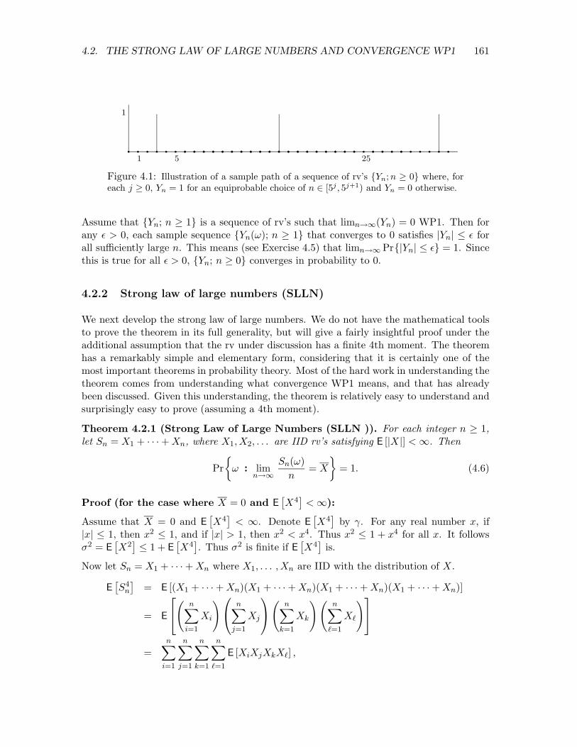
It is instructive to recall Example 1.5.1, illustrated in Figure 4.1, where {Yn; n ≥ 1} converges in probability but does not converge with probability one. Note that E [Yn] = 1/(5j+1 − 1) for n ∈ [5j , 5j+1). Thus limn→1 E [Yn] = 0, but

P1n=1 E [Yn] = 1. Thus

this sequence does not satisfy the conditions of the lemma. This helps explain how the conditions in the lemma exclude such sequences.

Before proceeding to the SLLN, we want to show that convergence WP1 implies convergence in probability. We give an incomplete argument here with precise versions both in Exercise 4.5 and Exercise 4.6. Exercise 4.6 has the added merit of expressing the set {ω : limn Yn(ω) = 0} explicitly in terms of countable unions and intersections of simple events involving finite sets of the Yn. This representation is valid whether or not the conditions of the lemma are satisfied and shows that this set is indeed an event.

4This proof probably appears to be somewhat nitpicking about limits. The reason for this is that the argument is quite abstract and it is difficult to develop the kind of intuition that ordinarily allows us to be somewhat more casual.

4.2. THE STRONG LAW OF LARGE NUMBERS AND CONVERGENCE WP1 161

1

q q q q q q q q q q q q q q q q q q q q q q q q qq q q q q q q q q q q q q q q q q q q q q q q qq q q q q q q q q1 5 25

Figure 4.1: Illustration of a sample path of a sequence of rv’s {Yn; n ≥ 0} where, for each j ≥ 0, Yn = 1 for an equiprobable choice of n ∈ [5j , 5j+1) and Yn = 0 otherwise.

Assume that {Yn; n ≥ 1} is a sequence of rv’s such that limn→1(Yn) = 0 WP1. Then for any ≤ > 0, each sample sequence {Yn(ω); n ≥ 1} that converges to 0 satisfies |Yn| ≤ ≤ for all sufficiently large n. This means (see Exercise 4.5) that limn→1 Pr{|Yn| ≤ ≤} = 1. Since this is true for all ≤ > 0, {Yn; n ≥ 0} converges in probability to 0.

4.2.2 Strong law of large numbers (SLLN)

We next develop the strong law of large numbers. We do not have the mathematical tools to prove the theorem in its full generality, but will give a fairly insightful proof under the additional assumption that the rv under discussion has a finite 4th moment. The theorem has a remarkably simple and elementary form, considering that it is certainly one of the most important theorems in probability theory. Most of the hard work in understanding the theorem comes from understanding what convergence WP1 means, and that has already been discussed. Given this understanding, the theorem is relatively easy to understand and surprisingly easy to prove (assuming a 4th moment).

Theorem 4.2.1 (Strong Law of Large Numbers (SLLN )). For each integer n ≥ 1, let Sn = X1 + · · · + Xn, where X1,X2, . . . are IID rv’s satisfying E [|X|] < 1. Then

Ω Sn(ω)

æPr ω : lim = X = 1. (4.6)

n→1 n

Proof (for the case where X = 0 and E £X4

§ < 1):

Assume that X = 0 and E £X4

§ < 1. Denote E

£X4

§ by ∞. For any real number x, if

|x| ≤ 1, then x2 ≤ 1, and if |x| > 1, then x2 < x4 . Thus x2 ≤ 1 + x4 for all x. It follows σ2 = E

£X2

§ ≤ 1 + E

£X4

§. Thus σ2 is finite if E

£X4

§ is.

Now let Sn = X1 + + Xn where X1, . . . ,Xn are IID with the distribution of X.· · ·

E £S4

§ = E [(X1 + + Xn)(X1 + + Xn)(X1 + + Xn)(X1 + + Xn)]n · · · · · · · · · · · ·

√ n

! n

√ n

!√ n

!

= E X

Xi X

Xj X

Xk

X X`

i=1 j=1 k=1 `=1

n n n n

= XXXX

E [XiXj XkX`] ,i=1 j=1 k=1 `=1


where we have multiplied out the product of sums to get a sum of n4 terms.

For each i, 1 ≤ i ≤ n, there is a term in this sum with i = j = k = `. For each such term, E [XiXj XkX`] = E

£X4

§ = ∞. There are n such terms (one for each choice of i, 1 ≤ i ≤ n)

and they collectively contribute n∞ to the sum E £Sn

4§. Also, for each i, k = i, there is a 6

term with j = i and ` = k. For each of these n(n − 1) terms, E [XiXiXkXk] = σ4 . There are another n(n − 1) terms with j =6 i and k = i, ` = j. Each such term contributes σ4 to the sum. Finally, for each i 6= j, there is a term with ` = i and k = j. Collectively all of these terms contribute 3n(n − 1)σ4 to the sum. Each of the remaining terms is 0 since at least one of i, j, k, is different from all the others, Thus we have

E £S4

§ = n∞ + 3n(n − 1)σ4 .n

Now consider the sequence of rv’s {Sn4/n4; n ≥ 1}.

1S4 ∏ 1

n∞ + 3n(n − 1)σ4X E

∑ØØØØ nn 4

ØØØØ = X

n4 < 1, n=1 n=1

where we have used the facts that the series P

n≥1 1/n2 and the series P

n≥1 1/n3 converge.

Using Lemma 4.2.1 applied to {S4/n4; n ≥ 1}, we see that limn→1 S4/n4 = 0 WP1. For n n

each ω such that limn→1 S4(ω)/n4 = 0, the nonnegative fourth root of that sequence of n

nonnegative numbers also approaches 0. Thus limn→1 |Sn/n| = 0 WP1.

The above proof assumed that E [X] = 0. It can be extended trivially to the case of an arbitrary finite X by replacing X in the proof with X − X. A proof using the weaker condition that σ2

X < 1 will be given in Section 7.9.1.

The technique that was used at the end of this proof provides a clue about why the concept of convergence WP1 is so powerful. The technique showed that if one sequence of rv’s ({Sn

4/n4; n ≥ 1}) converges to 0 WP1, then another sequence (|Sn/n|; n ≥ 1}) also converges WP1. We will formalize and generalize this technique in Lemma 4.3.2 as a major step toward establishing the strong law for renewal processes.

4.3 Strong law for renewal processes

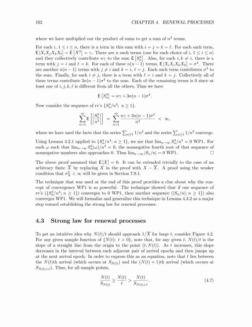
To get an intuitive idea why N(t)/t should approach 1/X for large t, consider Figure 4.2. For any given sample function of {N(t); t > 0}, note that, for any given t, N(t)/t is the slope of a straight line from the origin to the point (t,N(t)). As t increases, this slope decreases in the interval between each adjacent pair of arrival epochs and then jumps up at the next arrival epoch. In order to express this as an equation, note that t lies between the N(t)th arrival (which occurs at SN(t)) and the (N(t) + 1)th arrival (which occurs at SN(t)+1). Thus, for all sample points,

N(t) N(t) >

N(t) . (4.7)

SN(t) ≥

SN(t)+1 t

163 4.3. STRONG LAW FOR RENEWAL PROCESSES

✘✘✘✘✘✘✘✘✘✘✘✘✘✘✘✘✘✘✘✘❅

❅ ❅❘ ❄

Slope = N(t) t

Slope = N(t) SN(t)

Slope = N(t) SN(t)+1

❆ ❆❆

t

N(t)

0 S1 SN(t) SN(t)+1 N(t) N(t)Figure 4.2: Comparison of a sample function of N(t)/t with SN (t)

and SN(t)+1 for the

same sample point. Note that for the given sample point, N(t) is the number of arrivals up to and including t, and thus SN(t) is the epoch of the last arrival before or at time t. Similarly, SN(t)+1 is the epoch of the first arrival strictly after time t.

We want to show intuitively why the slope N(t)/t in the figure approaches 1/X as t → 1. As t increases, we would guess that N(t) increases without bound, i.e., that for each arrival, another arrival occurs eventually. Assuming this, the left side of (4.7) increases with increasing t as 1/S1, 2/S2, . . . , n/Sn, . . . , where n = N(t). Since Sn/n converges to X WP1 from the strong law of large numbers, we might be brave enough or insightful enough to guess that n/Sn converges to 1/X.

We are now ready to state the strong law for renewal processes as a theorem. Before proving the theorem, we formulate the above two guesses as lemmas and prove their validity.

Theorem 4.3.1 (Strong Law for Renewal Processes). For a renewal process with mean inter-renewal interval X < 1, limt→1 N(t)/t = 1/X WP1.

Lemma 4.3.1. Let {N(t); t > 0} be a renewal counting process with inter-renewal rv’s {Xn; n ≥ 1}. Then (whether or not X < 1), limt→1 N(t) = 1 WP1 and limt→1 E [N(t)] = 1.

Proof of Lemma 4.3.1: Note that for each sample point ω, N(t,ω) is a nondecreasing real-valued function of t and thus either has a finite limit or an infinite limit. Using (4.1), the probability that this limit is finite with value less than any given n is

lim Pr{N(t) < n} = lim Pr{Sn > t} = 1 − lim Pr{Sn ≤ t} . t→1 t→1 t→1

Since the Xi are rv’s, the sums Sn are also rv’s (i.e., nondefective) for each n (see Section 1.3.7), and thus limt→1 Pr{Sn ≤ t} = 1 for each n. Thus limt→1 Pr{N(t) < n} = 0 for each n. This shows that the set of sample points ω for which limt→1 N(t(ω)) < n has probability 0 for all n. Thus the set of sample points for which limt→1 N(t,ω) is finite has probability 0 and limt→1 N(t) = 1 WP1.

Next, E [N(t)] is nondecreasing in t, and thus has either a finite or infinite limit as t →1. For each n, Pr{N(t) ≥ n} ≥ 1/2 for large enough t, and therefore E [N(t)] ≥ n/2 for such t. Thus E [N(t)] can have no finite limit as t →1, and limt→1 E [N(t)] = 1.

The following lemma is quite a bit more general than the second guess above, but it will be useful elsewhere. This is the formalization of the technique used at the end of the proof of the SLLN.


Lemma 4.3.2. Let {Zn; n ≥ 1} be a sequence of rv’s such that limn→1 Zn = α WP1. Let f be a real valued function of a real variable that is continuous at α. Then

lim f(Zn) = f(α) WP1. (4.8) n→1

Proof of Lemma 4.3.2: First let z1, z2, . . . , be a sequence of real numbers such that limn→1 zn = α. Continuity of f at α means that for every ≤ > 0, there is a δ > 0 such that |f(z) − f(α)| < ≤ for all z such that |z − α| < δ. Also, since limn→1 zn = α, we know that for every δ > 0, there is an m such that |zn − α| ≤ δ for all n ≥ m. Putting these two statements together, we know that for every ≤ > 0, there is an m such that |f(zn)−f(α)| < ≤ for all n ≥ m. Thus limn→1 f(zn) = f(α).

If ω is any sample point such that limn→1 Zn(ω) = α, then limn→1 f(Zn(ω)) = f(α). Since this set of sample points has probability 1, (4.8) follows.

Proof of Theorem 4.3.1, Strong law for renewal processes: Since Pr{X > 0} = 1 for a renewal process, we see that X > 0. Choosing f(x) = 1/x, we see that f(x) is continuous at x = X. It follows from Lemma 4.3.2 that

n 1lim = WP1.

n→1 Sn X

From Lemma 4.3.1, we know that limt→1 N(t) = 1 with probability 1, so, with probability 1, N(t) increases through all the nonnegative integers as t increases from 0 to 1. Thus

N(t) n 1lim = lim = WP1. t→1 SN(t) n→1 Sn X

Recall that N(t)/t is sandwiched between N(t)/SN(t) and N(t)/SN(t)+1, so we can complete the proof by showing that limt→1 N(t)/SN(t)+1 = 1/X. To show this,

N(t) n n+1 n 1lim = lim = lim = WP1. t→1 SN(t)+1 n→1 Sn+1 n→1 Sn+1 n+1 X

We have gone through the proof of this theorem in great detail, since a number of the techniques are probably unfamiliar to many readers. If one reads the proof again, after becoming familiar with the details, the simplicity of the result will be quite striking. The theorem is also true if the mean inter-renewal interval is infinite; this can be seen by a truncation argument (see Exercise 4.8).

As explained in Section 4.2.1, Theorem 4.3.1 also implies the corresponding weak law of large numbers for N(t), i.e., for any ≤ > 0, limt→1 Pr

©|N(t)/t − 1/X| ≥ ≤

™ = 0). This

weak law could also be derived from the weak law of large numbers for Sn (Theorem 1.5.3). We do not pursue that here, since the derivation is tedious and uninstructive. As we will see, it is the strong law that is most useful for renewal processes.

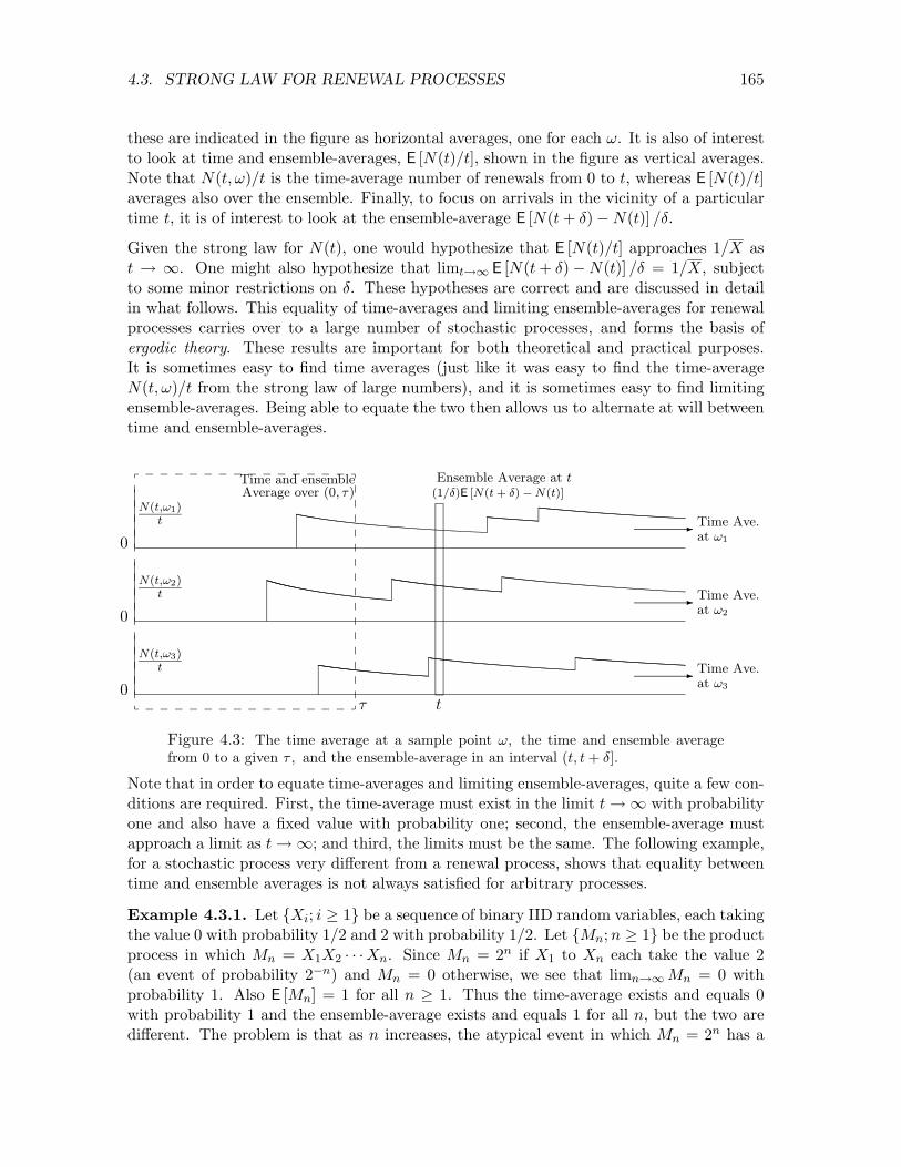
Figure 4.3 helps give some appreciation of what the strong law for N(t) says and doesn’t say. The strong law deals with time-averages, limt→1 N(t,ω)/t, for individual sample points ω;

165 4.3. STRONG LAW FOR RENEWAL PROCESSES

these are indicated in the figure as horizontal averages, one for each ω. It is also of interest to look at time and ensemble-averages, E [N(t)/t], shown in the figure as vertical averages. Note that N(t,ω)/t is the time-average number of renewals from 0 to t, whereas E [N(t)/t] averages also over the ensemble. Finally, to focus on arrivals in the vicinity of a particular time t, it is of interest to look at the ensemble-average E [N(t + δ) − N(t)] /δ.

Given the strong law for N(t), one would hypothesize that E [N(t)/t] approaches 1/X as t → 1. One might also hypothesize that limt→1 E [N(t + δ) − N(t)] /δ = 1/X, subject to some minor restrictions on δ. These hypotheses are correct and are discussed in detail in what follows. This equality of time-averages and limiting ensemble-averages for renewal processes carries over to a large number of stochastic processes, and forms the basis of ergodic theory. These results are important for both theoretical and practical purposes. It is sometimes easy to find time averages (just like it was easy to find the time-average N(t,ω)/t from the strong law of large numbers), and it is sometimes easy to find limiting ensemble-averages. Being able to equate the two then allows us to alternate at will between time and ensemble-averages.

0

0

0

N(t,ω1) t

N(t,ω2) t

N(t,ω3) t

Time and ensemble Average over (0, τ)

✲

✲

✲

Time Ave. at ω2

Time Ave. at ω1

Time Ave. at ω3

Ensemble Average at t (1/δ)E [N(t + δ) − N(t)]

τ t

Figure 4.3: The time average at a sample point ω, the time and ensemble average from 0 to a given τ , and the ensemble-average in an interval (t, t + δ].

Note that in order to equate time-averages and limiting ensemble-averages, quite a few conditions are required. First, the time-average must exist in the limit t →1 with probability one and also have a fixed value with probability one; second, the ensemble-average must approach a limit as t →1; and third, the limits must be the same. The following example, for a stochastic process very different from a renewal process, shows that equality between time and ensemble averages is not always satisfied for arbitrary processes.

Example 4.3.1. Let {Xi; i ≥ 1} be a sequence of binary IID random variables, each taking the value 0 with probability 1/2 and 2 with probability 1/2. Let {Mn; n ≥ 1} be the product process in which Mn = Xn. Since Mn = 2n if X1 to Xn each take the value 2 X1X2 · · · (an event of probability 2−n) and Mn = 0 otherwise, we see that limn→1 Mn = 0 with probability 1. Also E [Mn] = 1 for all n ≥ 1. Thus the time-average exists and equals 0 with probability 1 and the ensemble-average exists and equals 1 for all n, but the two are different. The problem is that as n increases, the atypical event in which Mn = 2n has a


probability approaching 0, but still has a significant effect on the ensemble-average.

Further discussion of ensemble averages is postponed to Section 4.6. Before that, we briefly state and discuss the central limit theorem for counting renewal processes and then introduce the notion of rewards associated with renewal processes.

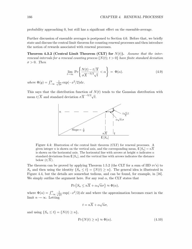
Theorem 4.3.2 (Central Limit Theorem (CLT) for N(t)). Assume that the inter-renewal intervals for a renewal counting process {N(t); t > 0} have finite standard deviation σ > 0. Then

(N(t) − t/X

)

lim Pr < α = Φ(α). (4.9)t→1 σX

−3/2√t

1where Φ(y) = R y exp(−x2/2)dx. −1

√2π

This says that the distribution function of N(t) tends to the Gaussian distribution with

mean t/X and standard deviation σX −3/2√

t.

✻❍ ❅ ❍ α

√n σ

n ✛ ✲❄❍■

❅ X

✟✟✟✟✟✟✟✟✟✟✟✟✟✟✟✟✟✟✟

α√

✟

n σ

Slope = 1 X

nX t E [Sn]

Figure 4.4: Illustration of the central limit theorem (CLT) for renewal processes. A given integer n is shown on the vertical axis, and the corresponding mean, E [Sn] = nX is shown on the horizontal axis. The horizontal line with arrows at height n indicates α standard deviations from E [Sn], and the vertical line with arrows indicates the distance below (t/X).

The theorem can be proved by applying Theorem 1.5.2 (the CLT for a sum of IID rv’s) to Sn and then using the identity {Sn ≤ t} = {N(t) ≥ n}. The general idea is illustrated in Figure 4.4, but the details are somewhat tedious, and can be found, for example, in [16]. We simply outline the argument here. For any real α, the CLT states that

Pr©Sn ≤ nX + α

√nσ

™ ≈ Φ(α),

1where Φ(α) = R α exp(−x2/2) dx and where the approximation becomes exact in the −1

√2π

limit n →1. Letting

t = nX + α√

nσ,

and using {Sn ≤ t} = {N(t) ≥ n},

Pr{N(t) ≥ n} ≈ Φ(α). (4.10)

167 4.4. RENEWAL-REWARD PROCESSES; TIME-AVERAGES

Since t is monotonic in n for fixed α, we can express n in terms of t, getting

t ασ√

n t n =

X −

X ≈

X − ασt1/2(X)−3/2 .

Substituting this into (4.10) establishes the theorem for −α, which establishes the theorem since α is arbitrary. The omitted details involve handling the approximations carefully.

4.4 Renewal-reward processes; time-averages

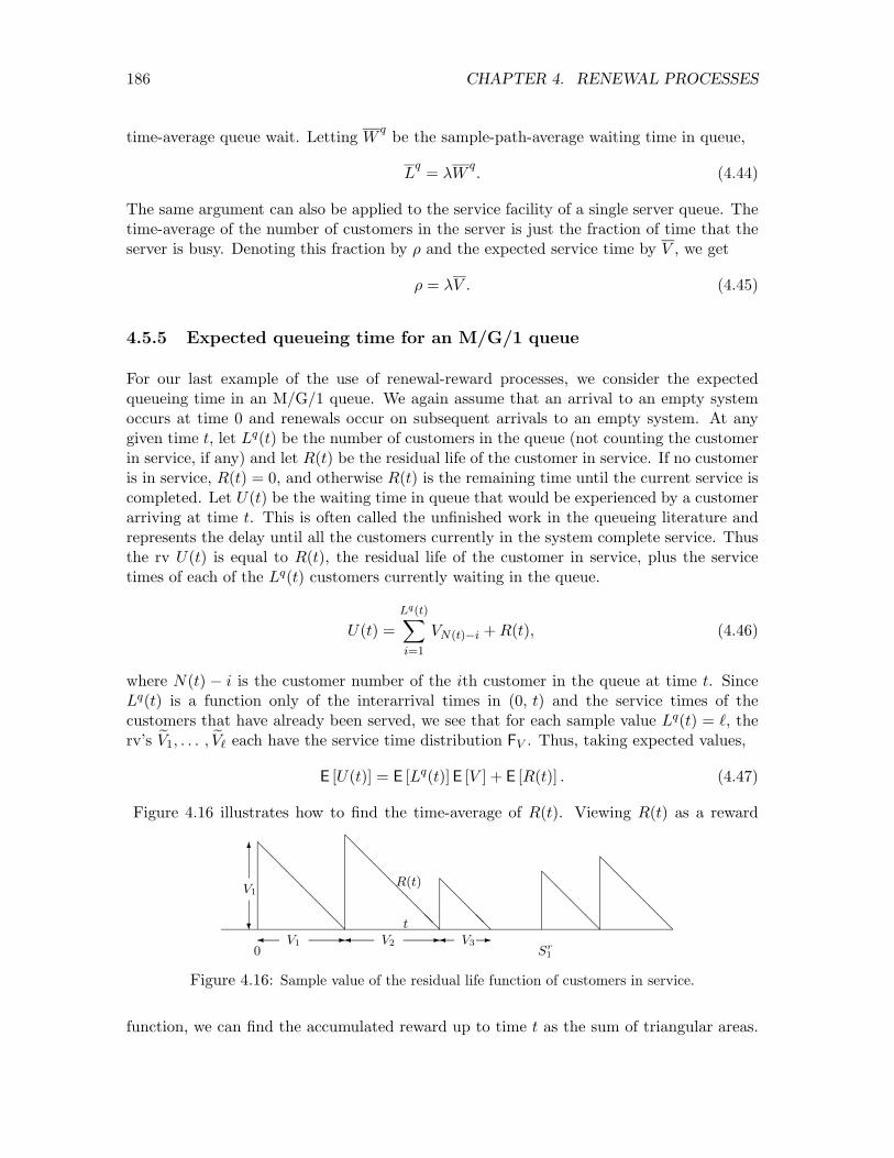
There are many situations in which, along with a renewal counting process {N(t); t > 0}, there is another randomly varying function of time, called a reward function {R(t); t > 0}. R(t) models a rate at which the process is accumulating a reward. We shall illustrate many examples of such processes and see that a “reward” could also be a cost or any randomly varying quantity of interest. The important restriction on these reward functions is that R(t) at a given t depends only on the location of t within the inter-renewal interval containing t and perhaps other random variables local to that interval. Before defining this precisely, we start with several examples.

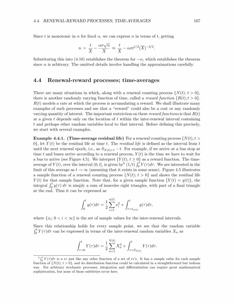
Example 4.4.1. (Time-average residual life) For a renewal counting process {N(t), t > 0}, let Y (t) be the residual life at time t. The residual life is defined as the interval from t until the next renewal epoch, i.e., as SN(t)+1 − t. For example, if we arrive at a bus stop at time t and buses arrive according to a renewal process, Y (t) is the time we have to wait for a bus to arrive (see Figure 4.5). We interpret {Y (t); t ≥ 0} as a reward function. The time-average of Y (t), over the interval (0, t], is given by5 (1/t)

R 0 t Y (τ)dτ . We are interested in the

limit of this average as t →1 (assuming that it exists in some sense). Figure 4.5 illustrates a sample function of a renewal counting process {N(t); t > 0} and shows the residual life Y (t) for that sample function. Note that, for a given sample function {Y (t) = y(t)}, the integral

R 0 t y(τ) dτ is simply a sum of isosceles right triangles, with part of a final triangle

at the end. Thus it can be expressed as

n(t)Z t

y(τ)dτ =1 X

x 2 i +

Z t

y(τ )dτ,20 i=1 τ=sn(t)

where {xi; 0 < i < 1} is the set of sample values for the inter-renewal intervals.

Since this relationship holds for every sample point, we see that the random variable R t Y (τ)dτ can be expressed in terms of the inter-renewal random variables Xn as

N(t)Z t

Y (τ)dτ =1 X

X2 + Z t

Y (τ )dτ.2 n

τ =0 n=1 τ =SN(t)

5R 0 t Y (τ)dτ is a rv just like any other function of a set of rv’s. It has a sample value for each sample

function of {N(t); t > 0}, and its distribution function could be calculated in a straightforward but tedious way. For arbitrary stochastic processes, integration and differentiation can require great mathematical sophistication, but none of those subtleties occur here.

0


X1

X2

N(t)

✲✛

S1 S2 S3 S4 S5 S6

X5❅

❅ ❅Y (t)X2 X4❅ ❅ ❅ X6❅ ❅X1 ❅ ❅ ❅ ❅ ❅X3 ❅ ❅ ❅ ❅ ❅ ❅ ❅ ❅ ❅ ❅ t ❅ ❅

S1 S2 S3 S4 S5 S6

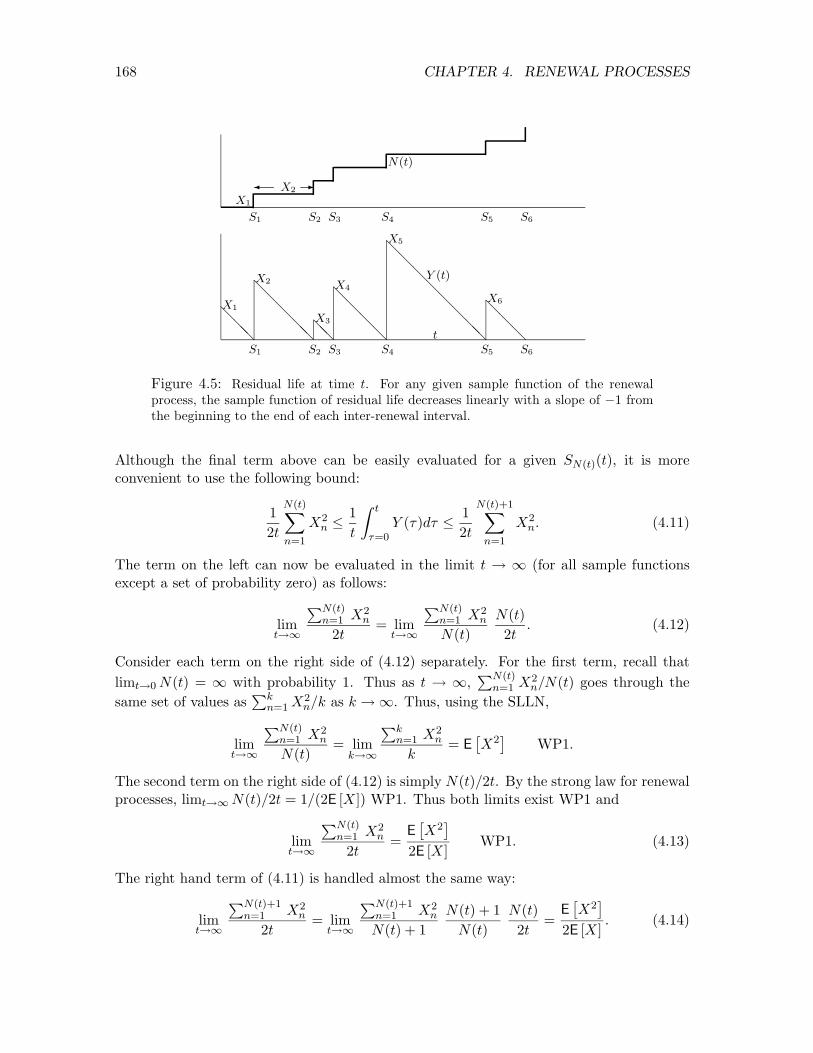
Figure 4.5: Residual life at time t. For any given sample function of the renewal process, the sample function of residual life decreases linearly with a slope of −1 from the beginning to the end of each inter-renewal interval.

Although the final term above can be easily evaluated for a given SN(t)(t), it is more convenient to use the following bound:

N(t) N(t)+11 X

X2 1 Z t

Y (τ)dτ ≤ 1 X

Xn2 . (4.11)

2t n ≤ t τ=0 2t

n=1 n=1

The term on the left can now be evaluated in the limit t → 1 (for all sample functions except a set of probability zero) as follows:

PN(t) X2 PN(t) X2 N(t)n=1 n n=1 nlim 2t

= lim N(t) 2t

. (4.12)t→1 t→1

Consider each term on the right side of (4.12) separately. For the first term, recall that PN(t)limt 0 N(t) = 1 with probability 1. Thus as t → 1, n=1 Xn2/N(t) goes through the →

same set of values as Pk

n=1 X2/k as k →1. Thus, using the SLLN, n

PN(t) X2 Pk X2 n=1 n n=1 n = E

£X2

§lim = lim WP1. t→1 N(t) k→1 k

The second term on the right side of (4.12) is simply N(t)/2t. By the strong law for renewal processes, limt→1 N(t)/2t = 1/(2E [X]) WP1. Thus both limits exist WP1 and

PN(t) X2 E £X2

§lim n=1 n = WP1. (4.13)t→1 2t 2E [X]

The right hand term of (4.11) is handled almost the same way: PN(t)+1 X2 PN(t)+1 X2 N(t) + 1 N(t) E

£X2

§lim n=1 n = lim n=1 n = (4.14)t→1 2t t→1 N(t) + 1 N(t) 2t 2E [X]

.

4.4. RENEWAL-REWARD PROCESSES; TIME-AVERAGES 169

Combining these two results, we see that, with probability 1, the time-average residual life is given by

R t E £X2

§lim τ=0 Y (τ) dτ

= (4.15)t→1 t 2E [X]

.

Note that this time-average depends on the second moment of X; this is X2 + σ2 ≥ X2 , so

the time-average residual life is at least half the expected inter-renewal interval (which is not surprising). On the other hand, the second moment of X can be arbitrarily large (even infinite) for any given value of E [X], so that the time-average residual life can be arbitrarily large relative to E [X]. This can be explained intuitively by observing that large inter-renewal intervals are weighted more heavily in this time-average than small inter-renewal intervals.

Example 4.4.2. As an example of the effect of improbable but large inter-renewal intervals, let X take on the value ≤ with probability 1 − ≤ and value 1/≤ with probability ≤. Then, for small ≤, E [X] ∼ 1, E

£X2

§ ∼ 1/≤, and the time average residual life is approximately 1/(2≤)

(see Figure 4.6).

❅❅❅❅❅❅❅❅❅

❅ ❅

❅ ❅

❅ ❅

❅ ❅

❅ ❅

❅ ❅❅❅❅❅❅

❅ ❅

❅ ❅

❅ ❅

1/≤

1/≤ ✲✛

Y (t)

✛✲ ≤

Figure 4.6: Average Residual life is dominated by large interarrival intervals. Each large interval has duration 1/≤, and the expected aggregate duration between successive large intervals is 1 − ≤

Example 4.4.3. (time-average Age) Let Z(t) be the age of a renewal process at time t where age is defined as the interval from the most recent arrival before (or at) t until t, i.e., Z(t) = t − SN(t). By convention, if no arrivals have occurred by time t, we take the age to be t (i.e., in this case, N(t) = 0 and we take S0 to be 0).

As seen in Figure 4.16, the age process, for a given sample function of the renewal process, is almost the same as the residual life process—the isosceles right triangles are simply turned around. Thus the same analysis as before can be used to show that the time average of Z(t) is the same as the time-average of the residual life,

R t Z(τ) dτ E £X2

§lim τ=0 = WP1. (4.16)t→1 t 2E [X]


° ° Z(t)°

° ° ° ° ° ° ° ° ° ° ° ° ° ° °

° ° °°° ° t ° S1 S2 S3 S4 S5 S6

Figure 4.7: Age at time t: For any given sample function of the renewal process, the sample function of age increases linearly with a slope of 1 from the beginning to the end of each inter-renewal interval.

Example 4.4.4. (time-average Duration) Let Xe(t) be the duration of the inter-renewal interval containing time t, i.e., X(t) = XN(t)+1 = SN(t)+1 − SN(t) (see Figure 4.8). It is e

clear that Xe(t) = Z(t) + Y (t), and thus the time-average of the duration is given by

lim

R τt =0 X

e(τ) dτ =

E £X2

§

WP1. (4.17)t→1 t E [X]

Again, long intervals are heavily weighted in this average, so that the time-average duration is at least as large as the mean inter-renewal interval and often much larger.

t

eX(t)

X5 ✲✛

S1 S2 S3 S4 S5 S6

Figure 4.8: Duration Xe(t) = XN(t) of the inter-renewal interval containing t.

4.4.1 General renewal-reward processes

In each of these examples, and in many other situations, we have a random function of time (i.e., Y (t), Z(t), or Xe(t)) whose value at time t depends only on where t is in the current inter-renewal interval (i.e., on the age Z(t) and the duration Xe(t) of the current inter-renewal interval). We now investigate the general class of reward functions for which the reward at time t depends at most on the age and the duration at t, i.e., the reward R(t) at time t is given explicitly as a function6 R(Z(t),Xe(t)) of the age and duration at t.

6This means that R(t) can be determined at any t from knowing Z(t) and X(t). It does not mean that R(t) must vary as either of those quantities are changed. Thus, for example, R(t) could depend on only one of the two or could even be a constant.

4.4. RENEWAL-REWARD PROCESSES; TIME-AVERAGES 171

For the three examples above, the function R is trivial. That is, the residual life, Y (t), is given by Xe(t) − Z(t) and the age and duration are given directly.

We now find the time-average value of R(t), namely, limt→1 1

R t R(τ) dτ . As in examples t 0 4.4.1 to 4.4.4 above, we first want to look at the accumulated reward over each inter-renewal period separately. Define Rn as the accumulated reward in the nth renewal interval,

Z Sn Z Sn

Rn = R(τ ) d(τ) = R[Z(τ),Xe(τ)] dτ. (4.18) Sn−1 Sn−1

For residual life (see Example 4.4.1), Rn is the area of the nth isosceles right triangle in Figure 4.5. In general, since Z(τ ) = τ − Sn−1,

Z Sn Z Xn

Rn = R(τ−Sn−1,Xn) dτ = R(z,Xn) dz. (4.19) Sn−1 z=0

Note that Rn is a function only of Xn, where the form of the function is determined by R(Z,X). From this, it is clear that {Rn; n ≥ 1} is essentially7 a set of IID random variables. For residual life, R(z,Xn) = Xn − z, so the integral in (4.19) is X2/2, as calculated by n

inspection before. In general, from (4.19), the expected value of Rn is given by

xZ 1 Z E [Rn] = R(z, x) dz dFX (x). (4.20)

x=0 z=0

Breaking R 0 t R(τ) dτ into the reward over the successive renewal periods, we get

Z t Z S1 Z S2

Z SN(t) Z t

R(τ) dτ = R(τ) dτ + R(τ) dτ + + R(τ) dτ + R(τ)dτ· · · 0 0 S1 SN(t)−1 SN(t)

N(t) Z t

= X

Rn + R(τ ) dτ. (4.21) n=1 SN(t)

The following theorem now generalizes the results of Examples 4.4.1, 4.4.3, and 4.4.4 to general renewal-reward functions.

Theorem 4.4.1. Let {R(t); t > 0} ≥ 0 be a nonnegative renewal-reward function for a renewal process with expected inter-renewal time E [X] = X < 1. If E [Rn] < 1, then with probability 1

t1 Z

E [Rn]lim R(τ) dτ = . (4.22)

τ=0t→1 t X

Proof: Using (4.21), the accumulated reward up to time t can be bounded between the accumulated reward up to the renewal before t and that to the next renewal after t,

PN(t) Rn R t R(τ) dτ

PN(t)+1 Rn . (4.23)n=1 τ=0 n=1

t ≤

t ≤

t 7One can certainly define functions R(Z, X) for which the integral in (4.19) is infinite or undefined for

some values of Xn, and thus Rn becomes a defective rv. It seems better to handle this type of situation when it arises rather than handling it in general.


The left hand side of (4.23) can now be broken into

PN(t) Rn PN(t) Rn N(t)n=1

t = n

N=1

(t) t. (4.24)

Each Rn is a given function of Xn, so the Rn are IID. As t →1, N(t) →1, and, thus, as we have seen before, the strong law of large numbers can be used on the first term on the right side of (4.24), getting E [Rn] with probability 1. Also the second term approaches 1/X by the strong law for renewal processes. Since 0 < X < 1 and E [Rn] is finite, the product of the two terms approaches the limit E [Rn] /X. The right-hand inequality of (4.23) is handled in almost the same way,

PN(t)+1 Rn PN(t)+1 Rn N(t) + 1 N(t)n=1 = n=1 . (4.25)

t N(t) + 1 N(t) t

It is seen that the terms on the right side of (4.25) approach limits as before and thus the term on the left approaches E [Rn] /X with probability 1. Since the upper and lower bound in (4.23) approach the same limit, (1/t)

R 0 t R(τ) dτ approaches the same limit and

the theorem is proved.

The restriction to nonnegative renewal-reward functions in Theorem 4.4.1 is slightly artificial. The same result holds for non-positive reward functions simply by changing the directions of the inequalities in (4.23). Assuming that E [Rn] exists (i.e., that both its positive and negative parts are finite), the same result applies in general by splitting an arbitrary reward function into a positive and negative part. This gives us the corollary:

Corollary 4.4.1. Let {R(t); t > 0} be a renewal-reward function for a renewal process with expected inter-renewal time E [X] = X < 1. If E [Rn] exists, then with probability 1

t1 Z

E [Rn]lim R(τ) dτ = . (4.26)t→1 t τ=0 X

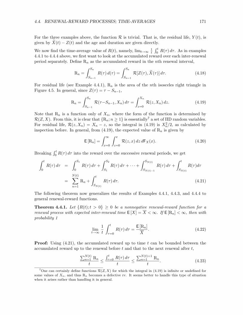
Example 4.4.5. (Distribution of Residual Life) Example 4.4.1 treated the time-average value of the residual life Y (t). Suppose, however, that we would like to find the time-average distribution function of Y (t), i.e., the fraction of time that Y (t) ≤ y as a function of y. The approach, which applies to a wide variety of applications, is to use an indicator function (for a given value of y) as a reward function. That is, define R(t) to have the value 1 for all t such that Y (t) ≤ y and to have the value 0 otherwise. Figure 4.9 illustrates this function for a given sample path. Expressing this reward function in terms of Z(t) and Xe(t), we have

( 1 ; X(t) − Z(t) ≤ y

R(t) = R(Z(t),Xe(t)) = e

. 0 ; otherwise

Note that if an inter-renewal interval is smaller than y (such as the third interval in Figure4.9), then R(t) has the value one over the entire interval, whereas if the interval is greater

173 4.4. RENEWAL-REWARD PROCESSES; TIME-AVERAGES

0 S1 S2 S3 S4

y

X3 ✲ ✛

✲✛ y ✲✛ y ✲✛

Figure 4.9: Reward function to find the time-average fraction of time that {Y (t) ≤ y}. For the sample function in the figure, X1 > y, X2 > y, and X4 > y, but X3 < y

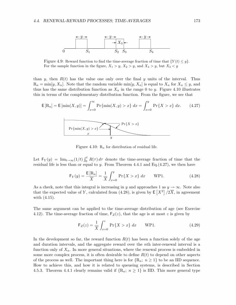
than y, then R(t) has the value one only over the final y units of the interval. Thus Rn = min[y,Xn]. Note that the random variable min[y,Xn] is equal to Xn for Xn ≤ y, and thus has the same distribution function as Xn in the range 0 to y. Figure 4.10 illustrates this in terms of the complementary distribution function. From the figure, we see that

Z 1 Z y

E [Rn] = E [min(X, y)] = Pr{min(X, y) > x} dx = Pr{X > x} dx. (4.27) x=0 x=0

Pr{X > x}Pr{min(X, y) > x} °°✠

✛ °°✒ ✲

x y

Figure 4.10: Rn for distribution of residual life.

Let FY (y) = limt→1(1/t) R t R(τ) dτ denote the time-average fraction of time that the0

residual life is less than or equal to y. From Theorem 4.4.1 and Eq.(4.27), we then have

E [Rn] 1 Z y

FY (y) = = Pr{X > x} dx WP1. (4.28)X X x=0

As a check, note that this integral is increasing in y and approaches 1 as y →1. Note also that the expected value of Y , calculated from (4.28), is given by E

£X2

§ /2X, in agreement

with (4.15).

The same argument can be applied to the time-average distribution of age (see Exercise 4.12). The time-average fraction of time, FZ (z), that the age is at most z is given by

z1 Z

FZ (z) = Pr{X > x} dx WP1. (4.29)X x=0

In the development so far, the reward function R(t) has been a function solely of the age and duration intervals, and the aggregate reward over the nth inter-renewal interval is a function only of Xn. In more general situations, where the renewal process is embedded in some more complex process, it is often desirable to define R(t) to depend on other aspects of the process as well. The important thing here is for {Rn; n ≥ 1} to be an IID sequence. How to achieve this, and how it is related to queueing systems, is described in Section 4.5.3. Theorem 4.4.1 clearly remains valid if {Rn; n ≥ 1} is IID. This more general type


of renewal-reward function will be required and further discussed in Sections 4.5.3 to Rss7 where we discuss Little’s theorem and the M/G/1 expected queueing delay, both of which use this more general structure.

Limiting time-averages are sometimes visualized by the following type of experiment. For some given large time t, let T be a uniformly distributed random variable over (0, t]; T is independent of the renewal-reward process under consideration. Then (1/t)

R 0 t R(τ) dτ is

the expected value (over T ) of R(T ) for a given sample path of {R(τ ); τ>0}. Theorem 4.4.1 states that in the limit t → 1, all sample paths (except a set of probability 0) yield the same expected value over T . This approach of viewing a time-average as a random choice of time is referred to as random incidence. Random incidence is awkward mathematically, since the random variable T changes with the overall time t and has no reasonable limit. It also blurs the distinction between time and ensemble-averages, so it will not be used in what follows.

4.5 Random stopping trials

Visualize performing an experiment repeatedly, observing independent successive sample outputs of a given random variable (i.e., observing a sample outcome of X1,X2, . . . where the Xi are IID). The experiment is stopped when enough data has been accumulated for the purposes at hand.

This type of situation occurs frequently in applications. For example, we might be required to make a choice from several hypotheses, and might repeat an experiment until the hypotheses are sufficiently discriminated. If the number of trials is allowed to depend on the outcome, the mean number of trials required to achieve a given error probability is typically a small fraction of the number of trials required when the number is chosen in advance. Another example occurs in tree searches where a path is explored until further extensions of the path appear to be unprofitable.

The first careful study of experimental situations where the number of trials depends on the data was made by the statistician Abraham Wald and led to the field of sequential analysis (see [21]). We study these situations now since one of the major results, Wald’s equality, will be useful in studying E [N(t)] in the next section. Stopping trials are frequently useful in the study of random processes, and in particular will be used in Section 4.7 for the analysis of queues, and again in Chapter 7 as central topics in the study of Random walks and martingales.

An important part of experiments that stop after a random number of trials is the rule for stopping. Such a rule must specify, for each sample path, the trial at which the experiment stops, i.e., the final trial after which no more trials are performed. Thus the rule for stopping should specify a positive, integer valued, random variable J , called the stopping time, or stopping trial, mapping sample paths to this final trial at which the experiment stops.

We view the sample space as including the set of sample value sequences for the never-ending sequence of random variables X1,X2, . . . . That is, even if the experiment is stopped at the end of the second trial, we still visualize the 3rd, 4th, . . . random variables as having sample

175 4.5. RANDOM STOPPING TRIALS

values as part of the sample function. In other words, we visualize that the experiment continues forever, but that the observer stops watching at the end of the stopping point. From the standpoint of applications, the experiment might or might not continue after the observer stops watching. From a mathematical standpoint, however, it is far preferable to view the experiment as continuing. This avoids confusion and ambiguity about the meaning of IID rv’s when the very existence of later variables depends on earlier sample values.

The intuitive notion of stopping a sequential experiment should involve stopping based on the data (i.e., the sample values) gathered up to and including the stopping point. For example, if X1,X2, . . . , represent the succesive changes in our fortune when gambling, we might want to stop when our cumulative gain exceeds some fixed value. The stopping trial n then depends on the sample values of X1,X2, . . . ,Xn. At the same time, we want to exclude from stopping trials those rules that allow the experimenter to peek at subsequent values before making the decision to stop or not.8 This leads to the following definition.

Definition 4.5.1. A stopping trial (or stopping time9) J for a sequence of rv’s X1,X2, . . . , is a positive integer-valued rv such that for each n ≥ 1, the indicator rv I{J=n} is a function of {X1,X2, . . . ,Xn}.

The last clause of the definition means that any given sample value x1, . . . , xn for X1, . . . ,Xn

uniquely determines whether the corresponding sample value of J is n or not. Note that since the stopping trial J is defined to be a positive integer-valued rv, the events {J = n}and {J = m} for m < n are disjoint events, so stopping at trial m makes it impossible to also stop at n for a given sample path. Also the union of the events {J = n} over n ≥ 1 has probability 1. Aside from this final restriction, the definition does not depend on the probability measure and depends solely on the set of events {J = n} for each n. In many situations, it is useful to relax the definition further to allow J to be a possibly-defective rv. In this case the question of whether stopping occurs with probability 1 can be postponed until after specifying the disjoint events {J = n} over n ≥ 1.

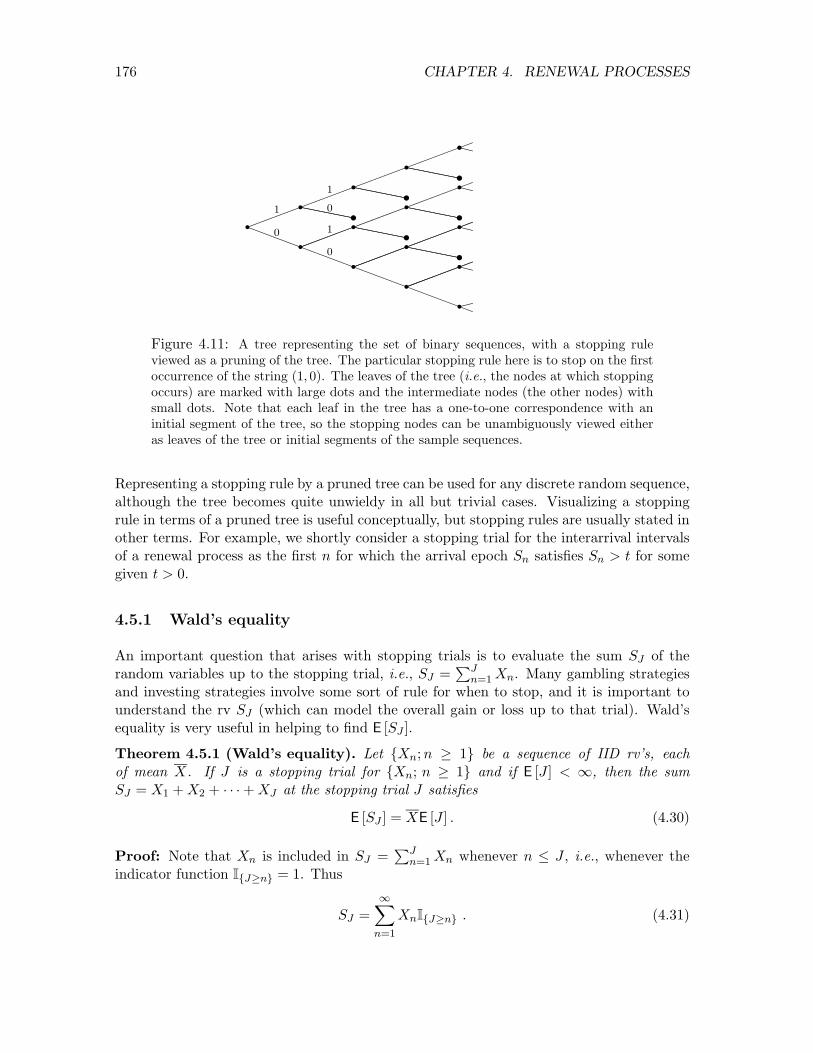
Example 4.5.1. Consider a Bernoulli process {Xn; n ≥ 1}. A very simple stopping trial for this process is to stop at the first occurrence of the string (1, 0). Figure 4.11 illustrates this stopping trial by viewing it as a truncation of the tree of possible binary sequences.

The event {J = 2}, i.e., the event that stopping occurs at trial 2, is the event {X1=1, X2=0}. Similarly, the event {J = 3} is {X1=1, X2=1, X3=0}

S{X1=0, X2=1, X3=0}. The dis

jointness of {J = n} and {J = m} for n =6 m is represented in the figure by terminating the tree at each stopping node. It can be seen that the tree never dies out completely, and in fact, for each trial n, the number of stopping nodes is n − 1. However, the probability that stopping has not occurred by trial n goes to zero exponentially with n, which ensures that J is a random variable.

8For example, poker players do not take kindly to a player who attempts to withdraw his bet when someone else wins the hand. Similarly, a statistician gathering data on product failures should not respond to a failure by then recording an earlier trial as a stopping time, thus not recording the failure.

9Stopping trials are more often called stopping times or optional stopping times in the literature. In our first major application of a stopping trial, however, the stopping trial is the first trial n at which a renewal epoch Sn exceeds a given time t . Viewing this trial as a time generates considerable confusion.


rr r sr sr r1 r 01 ssrr rs r0 1 r

0 sr r r r✘

Figure 4.11: A tree representing the set of binary sequences, with a stopping rule viewed as a pruning of the tree. The particular stopping rule here is to stop on the first occurrence of the string (1, 0). The leaves of the tree (i.e., the nodes at which stopping occurs) are marked with large dots and the intermediate nodes (the other nodes) with small dots. Note that each leaf in the tree has a one-to-one correspondence with an initial segment of the tree, so the stopping nodes can be unambiguously viewed either as leaves of the tree or initial segments of the sample sequences.

Representing a stopping rule by a pruned tree can be used for any discrete random sequence, although the tree becomes quite unwieldy in all but trivial cases. Visualizing a stopping rule in terms of a pruned tree is useful conceptually, but stopping rules are usually stated in other terms. For example, we shortly consider a stopping trial for the interarrival intervals of a renewal process as the first n for which the arrival epoch Sn satisfies Sn > t for some given t > 0.

4.5.1 Wald’s equality

An important question that arises with stopping trials is to evaluate the sum SJ of the random variables up to the stopping trial, i.e., SJ =

PJn=1 Xn. Many gambling strategies

and investing strategies involve some sort of rule for when to stop, and it is important to understand the rv SJ (which can model the overall gain or loss up to that trial). Wald’s equality is very useful in helping to find E [SJ ].

Theorem 4.5.1 (Wald’s equality). Let {Xn; n ≥ 1} be a sequence of IID rv’s, each of mean X. If J is a stopping trial for {Xn; n ≥ 1} and if E [J ] < 1, then the sum SJ = X1 + X2 + + XJ at the stopping trial J satisfies· · ·

E [SJ ] = XE [J ] . (4.30)

Proof: Note that Xn is included in SJ = PJ Xn whenever n ≤ J , i.e., whenever the n=1

indicator function I = 1. Thus{J≥n}

1SJ =

X XnI{J≥n} . (4.31)

n=1


This includes Xn as part of the sum if stopping has not occurred before trial n. The event {J ≥ n} is the complement of {J < n} = {J = 1}

S S{J = n − 1}. All of these latter · · ·

events are determined by X1, . . . ,Xn−1 and are thus independent of Xn. It follows that Xn

and {J < n} are independent and thus Xn and {J ≥ n} are also independent.10 Thus

E £XnI

§ = XE

£I

§ .{J≥n} {J≥n}

We then have hX1 i

E [SJ ] = E n=1

XnI{J≥n}

= X1

E £XnI

§ (4.32)

n=1 {J≥n}

= X1

XE £I

§n=1 {J≥n}

= XE [J ] . (4.33)

The interchange of expectation and infinite sum in (4.32) is obviously valid for a finite sum, and is shown in Exercise 4.18 to be valid for an infinite sum if E [J ] < 1. The example below shows that Wald’s equality can be invalid when E [J ] = 1. The final step above comes from the observation that E

£I

§ = Pr{J ≥ n}. Since J is a positive integer rv, {J≥n}

E [J ] = P1

n=1 Pr{J ≥ n}. One can also obtain the last step by using J = P1

n=1 I{J≥n} (see Exercise 4.13).

What this result essentially says in terms of gambling is that strategies for when to stop betting are not really effective as far as the mean is concerned. This sometimes appears obvious and sometimes appears very surprising, depending on the application.

Example 4.5.2 (Stop when you’re ahead in coin tossing). We can model a (biased) coin tossing game as a sequence of IID rv’s X1,X2, . . . where each X is 1 with probability p and −1 with probability 1 − p. Consider the possibly-defective stopping trial J where J is the first n for which Sn = X1 + + Xn = 1, i.e., the first trial at which the gambler is · · · ahead.

We first want to see if J is a rv, i.e., if the probability of eventual stopping, say θ = Pr{J < 1}, is 1. We solve this by a frequently useful trick, but will use other more systematic approaches in Chapters 5 and 7 when we look at this same example as a birth-death Markov chain and then as a simple random walk. Note that Pr{J = 1} = p, i.e., S1 = 1 with probability p and stopping occurs at trial 1. With probability 1 − p, S1 = −1. Following S1 = −1, the only way to become one ahead is to first return to Sn = 0 for some n > 1, and, after the first such return, go on to Sm = 1 at some later trial m. The probability of eventually going from -1 to 0 is the same as that of going from 0 to 1, i.e., θ. Also, given a first return to 0 from -1, the probability of reaching 1 from 0 is θ. Thus,

θ = p + (1 − p)θ2 .

10This can be quite confusing initially, since (as seen in the example of Figure 4.11) Xn is not necessarily independent of the event {J = n}, nor of {J = n + 1}, etc. In other words, given that stopping has not occurred before trial n, then Xn can have a great deal to do with the trial at which stopping occurs. However, as shown above, Xn has nothing to do with whether {J < n} or {J ≥ n}.


This is a quadratic equation in θ with two solutions, θ = 1 and θ = p/(1 − p). For p > 1/2, the second solution is impossible since θ is a probability. Thus we conclude that J is a rv. For p = 1/2 (and this is the most interesting case), both solutions are the same, θ = 1, and again J is a rv. For p < 1/2, the correct solution11 is θ = p/(1 − p). Thus θ < 1 so J is a defective rv.

For the cases where p ≥ 1/2, i.e., where J is a rv, we can use the same trick to evaluate E [J ],

E [J ] = p + (1 − p)(1 + 2E [J ]).

The solution to this is 1 1

E [J ] = = 2(1 − p) 2p − 1

.

We see that E [J ] is finite for p > 1/2 and infinite for p = 1/2.

For p > 1/2, we can check that these results agree with Wald’s equality. In particular, since SJ is 1 with probability 1, we also have E [SJ ] = 1. Since X = 2p − 1 and E [J ] = 1/(2p − 1), Wald’s equality is satisfied (which of course it has to be).

For p = 1/2, we still have SJ = 1 with probability 1 and thus E [SJ ] = 1. However X = 0 so XE [J ] has no meaning and Wald’s equality breaks down. Thus we see that the restriction E [J ] < 1 in Wald’s equality is indeed needed. These results are tabulated below.

p > 12 p = 12 p < 12

p .Pr{J < 1} 1 11−p

1E [J ] 2p−11 1

It is surprising that with p = 1/2, the gambler can eventually become one ahead with probability 1. This has little practical value, first because the required expected number of trials is infinite, and second (as will be seen later) because the gambler must risk a potentially infinite capital.

4.5.2 Applying Wald’s equality to m(t) = E [N(t)]

Let {Sn; n ≥ 1} be the arrival epochs and {Xn; n ≥ 1} the interarrival intervals for a renewal process. For any given t > 0, let J be the trial n for which Sn first exceeds t. Note that n is specified by the sample values of {X1, . . . ,Xn} and thus J is a possibly-defective stopping trial for {Xn; n ≥ 1}.

Since n is the first trial for which Sn > t, we see that Sn−1 ≤ t and Sn > t. Thus N(t) is n − 1 and n is the sample value of N(t) + 1. Since this is true for all sample sequences, J = N(t) + 1. Since N(t) is a non-defective rv, J is also, so J is a stopping trial for {Xn; n ≥ 1}.

11This will be shown when we view this example as a birth-death Markov chain in Chapter 5.


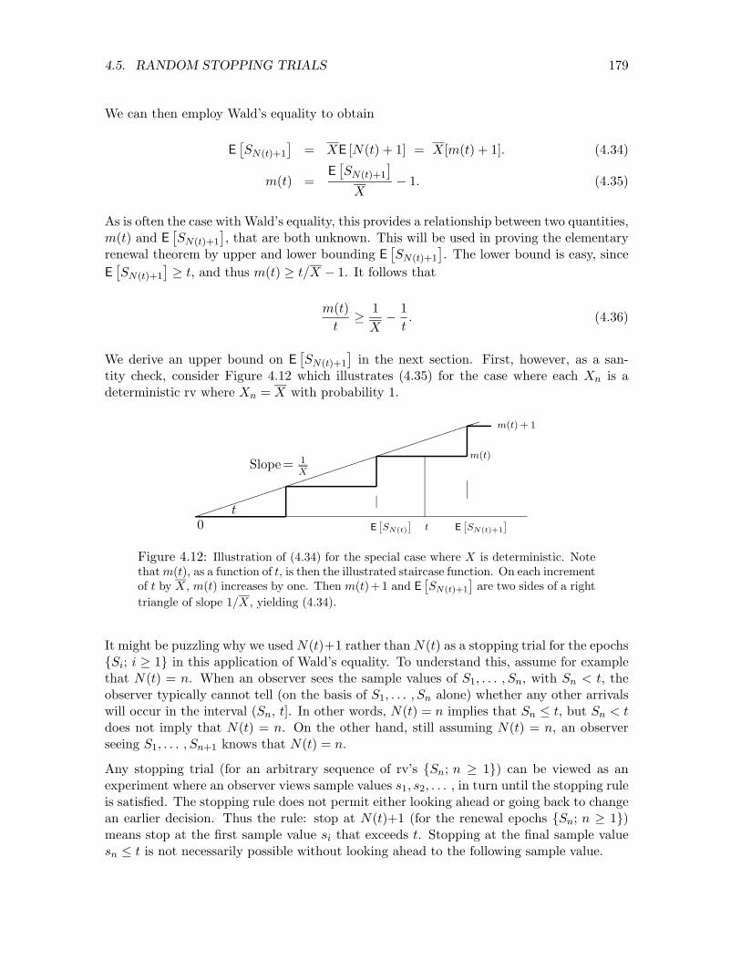
We can then employ Wald’s equality to obtain

E £SN(t)+1

§ = XE [N(t) + 1] = X[m(t) + 1]. (4.34)

E £SN(t)+1

§m(t) = − 1. (4.35)

X

As is often the case with Wald’s equality, this provides a relationship between two quantities, m(t) and E

£SN(t)+1

§, that are both unknown. This will be used in proving the elementary

renewal theorem by upper and lower bounding E £SN(t)+1

§. The lower bound is easy, since

E £SN(t)+1

§ ≥ t, and thus m(t) ≥ t/X − 1. It follows that

m(t) 1 1 t ≥

X −

t. (4.36)

We derive an upper bound on E £SN(t)+1

§ in the next section. First, however, as a san

tity check, consider Figure 4.12 which illustrates (4.35) for the case where each Xn is a deterministic rv where Xn = X with probability 1.

✏✏✏✏✏✏✏✏✏✏✏✏✏✏✏✏✏✏✏✏✏✏✏✏

Slope = 1 X

t

m(t)

m(t) + 1

0 E £SN(t)

§ t E

£SN (t)+1

§

Figure 4.12: Illustration of (4.34) for the special case where X is deterministic. Note that m(t), as a function of t, is then the illustrated staircase function. On each increment of t by X, m(t) increases by one. Then m(t)+1 and E

£SN(t)+1

§ are two sides of a right

triangle of slope 1/X, yielding (4.34).

It might be puzzling why we used N(t)+1 rather than N(t) as a stopping trial for the epochs {Si; i ≥ 1} in this application of Wald’s equality. To understand this, assume for example that N(t) = n. When an observer sees the sample values of S1, . . . , Sn, with Sn < t, the observer typically cannot tell (on the basis of S1, . . . , Sn alone) whether any other arrivals will occur in the interval (Sn, t]. In other words, N(t) = n implies that Sn ≤ t, but Sn < t does not imply that N(t) = n. On the other hand, still assuming N(t) = n, an observer seeing S1, . . . , Sn+1 knows that N(t) = n.

Any stopping trial (for an arbitrary sequence of rv’s {Sn; n ≥ 1}) can be viewed as an experiment where an observer views sample values s1, s2, . . . , in turn until the stopping rule is satisfied. The stopping rule does not permit either looking ahead or going back to change an earlier decision. Thus the rule: stop at N(t)+1 (for the renewal epochs {Sn; n ≥ 1}) means stop at the first sample value si that exceeds t. Stopping at the final sample value sn ≤ t is not necessarily possible without looking ahead to the following sample value.


4.5.3 Stopping trials, embedded renewals, and G/G/1 queues

The above definition of a stopping trial is quite restrictive in that it refers only to a single sequence of rv’s. In many queueing situations, for example, there is both a sequence of interarrival times {Xi; i ≥ 1} and a sequence of service times {Vi; i ≥ 0}. Here Xi is the interarrival interval between customer i − 1 and i, where an initial customer 0 is assumed to arrive at time 0, and X1 is the arrival time for customer 1. The service time of customer 0 is then V0 and each Vi, i > 0 is the service time of the corresponding ordinary customer. Customer number 0 is not ordinary in the sense that it arrives at the fixed time 0 and is not counted in the arrival counting process {N(t); t > 0}.

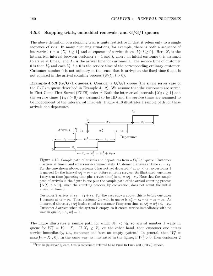
Example 4.5.3 (G/G/1 queues:). Consider a G/G/1 queue (the single server case of the G/G/m queue described in Example 4.1.2). We assume that the customers are served in First-Come-First-Served (FCFS) order.12 Both the interarrival intervals {Xi; i ≥ 1} and the service times {Vi; i ≥ 0} are assumed to be IID and the service times are assumed to be independent of the interarrival intervals. Figure 4.13 illustrates a sample path for these arrivals and departures.

s3

Arrivals

Departures0 2

3 s1

s2

v0 ✲✛

v1 ✲✛

v2 ✲✛

v3 ✲✛

x1 ✲✛

x2 ✲✛

x3 ✲✛

wq 1 ✲✛

wq 2 ✲✛

x2 + wq = wq 1 + v1✛ ✲

1

0

2

Figure 4.13: Sample path of arrivals and departures from a G/G/1 queue. Customer 0 arrives at time 0 and enters service immediately. Customer 1 arrives at time s1 = x1. For the case shown above, customer 0 has not yet departed, i.e., x1 < v0, so customer 1 is queued for the interval w

q = v0 − x1 before entering service. As illustrated, customer

1’s system time (queueing time plus service time) is w1

q 1

+v1. Note that the sample = w1 path of arrivals in the figure is one plus the sample path of the arrival counting process {N(t); t > 0}, since the counting process, by convention, does not count the initial arrival at time 0.

Customer 2 arrives at s2 = x1 + x2. For the case shown above, this is before customer 1 departs at v0 + v1. Thus, customer 2’s wait in queue is w2

q Asqq

= v0 + v1 − x1 − x2. is also equal to customer 1’s system time, so w2illustrated above, x2 +wq +v1 −x2.

Customer 3 arrives when the system is empty, so it enters service immediately with no = w12

wait in queue, i.e., wq 3 = 0.

The figure illustrates a sample path for which X1 < V0, so arrival number 1 waits in queue for W1

q = V0 − X1. If X1 ≥ V0, on the other hand, then customer one enters service immediately, i.e., customer one ‘sees an empty system.’ In general, then W1

q = max(V0 − X1, 0). In the same way, as illustrated in the figure, if W q > 0, then customer 2 1

12For single server queues, this is sometimes referred to as First-In-First-Out (FIFO) service.


waits for W q + V1 − X2 if positive and 0 otherwise. This same formula works if W q = 0, so 1 1 W2

q = max(W1 q + V1 − X2, 0). In general, it can be seen that

Wiq = max(Wi

q −1 + Vi−1 − Xi, 0). (4.37)

This equation will be analyzed further in Section 7.2 where we are interested in queueing delay and system delay. Here our objectives are simpler, since we only want to show that the subsequence of customer arrivals i for which the event {W q = 0} is satisfied form the i renewal epochs of a renewal process. To do this, first observe from (4.37) (using induction if desired) that W q is a function of (X1, . . . ,Xi) and (V0, . . . , Vi−1). Thus, if we let J be the i smallest i > 0 for which W q = 0, then IJ=i is a function of (X1, . . . ,Xi) and (V0, . . . , Vi−1).i

We now interrupt the discussion of G/G/1 queues with the following generalization of the definition of a stopping trial.

Definition 4.5.2 (Generalized stopping trials). A generalized stopping trial J for a sequence of pairs of rv’s (X1, V1), (X2, V2) . . . , is a positive integer-valued rv such that, for each n ≥ 1, the indicator rv I{J=n} is a function of X1, V1,X2, V2, . . . ,Xn, Vn.

Wald’s equality can be trivially generalized for these generalized stopping trials.

Theorem 4.5.2 (Generalized Wald’s equality). Let {(Xn, Vn); n ≥ 1} be a sequence of pairs of rv’s, where each pair is independent and identically distributed (IID) to all other pairs. Assume that each Xi has finite mean X. If J is a stopping trial for {(Xn, Vn); n ≥ 1}and if E [J ] < 1, then the sum SJ = X1 + X2 + + XJ satisfies· · ·

E [SJ ] = XE [J ] . (4.38)

The proof of this will be omitted, since it is the same as the proof of Theorem 4.5.1. In fact, the definition of stopping trials could be further generalized by replacing the rv’s Vi

by vector rv’s or by a random number of rv’s , and Wald’s equality would still hold.13

For the example of the G/G/1 queue, we take the sequence of pairs to be {(X1, V0), (X2, V1), . . . , }. Then {(Xn, Vn−1; n ≥ 1} satisfies the conditions of Theorem 4.5.2 (assuming that E [Xi] < 1). Let J be the generalized stopping rule specifying the number of the first arrival to find an empty queue. Then the theorem relates E [SJ ], the expected time t > 0 until the first arrival to see an empty queue, and E [J ], the expected number of arrivals until seeing an empty queue.

It is important here, as in many applications, to avoid the confusion created by viewing J as a stopping time. We have seen that J is the number of the first customer to see an empty queue, and SJ is the time until that customer arrives.

There is a further possible timing confusion about whether a customer’s service time is determined when the customer arrives or when it completes service. This makes no difference, since the ordered sequence of pairs is well-defined and satisfies the appropriate IID condition for using the Wald equality.

13In fact, J is sometimes defined to be a stopping rule if I{J≥n} is independent of Xn, Xn+1, . . . for each n. This makes it easy to prove Wald’s equality, but quite hard to see when the definition holds, especially since I{J=n}, for example, is typically dependent on Xn (see footnote 7).


As is often the case with Wald’s equality, it is not obvious how to compute either quantity in (4.38), but it is nice to know that they are so simply related. It is also interesting to see that, although successive pairs (Xi, Vi) are assumed independent, it is not necessary for Xi and Vi to be independent. This lack of independence does not occur for the G/G/1 (or G/G/m) queue, but can be useful in situations such as packet networks where the interarrival time between two packets at a given node can depend on the service time (the length) of the first packet if both packets are coming from the same node.

Perhaps a more important aspect of viewing the first renewal for the G/G/1 queue as a stopping trial is the ability to show that successive renewals are in fact IID. Let X2,1,X2,2, . . . be the interarrival times following J , the first arrival to see an empty queue. Conditioning on J = j, we have X2,1 =Xj+1, X2,2 =Xj+2, . . . ,. Thus {X2,k; k ≥ 1} is an IID sequence with the original interarrival distribution. Similarly {(X2,k, V2,k); k ≥ 1} is a sequence of IID pairs with the original distribution. This is valid for all sample values j of the stopping trial J . Thus {(X2,k, V2,k); k ≥ 1} is statistically independent of J and (Xi, Vi); 1 ≤ i ≤ J .

The argument above can be repeated for subsequent arrivals to an empty system, so we have shown that successive arrivals to an empty system actually form a renewal process.14

One can define many different stopping rules for queues, such as the first trial at which a given number of customers are in the queue. Wald’s equality can be applied to any such stopping rule, but much more is required for the stopping trial to also form a renewal point. At the first time when n customers are in the system, the subsequent departure times depend partly on the old service times and partly on the new arrival and service times, so the required independence for a renewal point does not exist. Stopping rules are helpful in understanding embedded renewal points, but are by no means equivalent to embedded renewal points.

Finally, nothing in the argument above for the G/G/1 queue made any use of the FCFS service discipline. One can use any service discipline for which the choice of which customer to serve at a given time t is based solely on the arrival and service times of customers in the system by time t. In fact, if the server is never idle when customers are in the system, the renewal epochs will not depend on the service descipline. It is also possible to extend these arguments to the G/G/m queue, although the service discipline can affect the renewal points in this case.

4.5.4 Little’s theorem

Little’s theorem is an important queueing result stating that the expected number of customers in a queueing system is equal to the product of the arrival rate and the expected time each customer waits in the system. This result is true under very general conditions; we use the G/G/1 queue with FCFS service as a specific example, but the reason for the greater generality will be clear as we proceed. Note that the theorem does not tell us how

14Confession by author: For about 15 years, I mistakenly believed that it was obvious that arrivals to an empty system in a G/G/m queue form a renewal process. Thus I can not expect readers to be excited about the above proof. However, it is a nice example of how to use stopping times to see otherwise murky points clearly.


to find either the expected number or expected wait; it only says that if one can be found, the other can also be found.

d(τ )

a(τ )

s2

s1

s3

w0 ✲✛

w1 ✲✛

w2 ✲✛

w3 ✲✛ ♣♣♣ ♣♣♣ ♣♣♣ ♣♣♣ ♣♣♣ ♣♣♣ ♣♣♣ ♣♣♣

0 s r 1 t s r

2

Figure 4.14: Sample path of arrivals, departures, and system waiting times for a G/G/1 queue with FCFS service. The upper step function is the number of customer arrivals, including the customer at time 0 and is denoted a(τ). Thus a(τ) is a sample path of A(τ ) = N(τ) + 1, i.e., the arrival counting process incremented by 1 for the initial arrival at τ = 0. The lower step function, d(τ) is a sample path for D(τ), which is the number of departures (including customer 0) up to time τ . For each i ≥ 0, wi is the sample value of the system waiting time Wi for customer i. Note that Wi = Wi

q + Vi. r rThe figure also shows the sample values s1 and s2 of the first two arrivals that see an

empty system (recall from Section 4.5.3 that the subsequence of arrivals that see an empty system forms a renewal process.)

Figure 4.14 illustrates a sample path for a G/G/1 queue with FCFS service. It illustrates a sample path a(t) for the arrival process A(t) = N(t) + 1, i.e., the number of customer arrivals in [0, t], specifically including customer number 0 arriving at t = 0. Similarly, it illustrates the departure process D(t), which is the number of departures up to time t, again including customer 0. The difference, L(t) = A(t) − D(t), is then the number in the system at time t.

Recall from Section 4.5.3 that the subsequence of customer arrivals for t > 0 that see an empty system form a renewal process. Actually, we showed a little more than that. Not only are the inter-renewal intervals, Xr = Si

r − Sir −1 IID, but the number of customer arrivals ini

each inter-renewal interval are IID, and the interarrival intervals and service times between r rinter-renewal intervals are IID. The sample values, s1 and s2 of the first two renewal epochs

are shown in the figure.

The essence of Little’s theorem can be seen by observing that R 0 Sr

L(τ) dτ in the figure is1

the area between the upper and lower step functions, integrated out to the first time that the two step functions become equal (i.e., the system becomes empty). For the sample value in the figure, this integral is equal to w0 + w1 + w2. In terms of the rv’s,

rZ S N(S1 r)−1

1

L(τ) dτ = X

Wi. (4.39) 0 i=0

The same relationship exists in each inter-renewal interval, and in particular we can define


Ln for each n ≥ 1 as Z Sr N(Sn

r )−1 n

Ln = L(τ) dτ = X

Wi. (4.40) Sr

n−1 i=N(Snr −1)

The interpretation of this is far simpler than the notation. The arrival step function and the departure step function in Figure 4.14 are separated whenever there are customers in the system (the system is busy) and are equal whenever the system is empty. Renewals occur when the system goes from empty to busy, so the nth renewal is at the beginning of the nth busy period. Then Ln is the area of the region between the two step functions over the nth busy period. By simple geometry, this area is also the sum of the customer waiting times over that busy period. Finally, since the interarrival intervals and service times in each busy period are IID with respect to those in each other busy period, the sequence L1, L2, . . . , is a sequence of IID rv’s.

The function L(τ) has the same behavior as a renewal reward function, but it is slightly more general, being a function of more than the age and duration of the renewal counting process {N r(t); t > 0} at t = τ . However the fact that {Ln; n ≥ 1} is an IID sequence lets us use the same methodology to treat L(τ) as was used earlier to treat renewal-reward functions. We now state and prove Little’s theorem. The proof is almost the same as that of Theorem 4.4.1, so we will not dwell on it.

Theorem 4.5.3 (Little). For a FCFS G/G/1 queue in which the expected inter-renewal interval is finite, the limiting time-average number of customers in the system is equal, with probability 1, to a constant denoted as L. The sample-path-average waiting time per customer is also equal, with probability 1, to a constant denoted as W . Finally L = ∏W where ∏ is the customer arrival rate, i.e., the reciprocal of the expected interarrival time.

Proof: Note that for any t > 0, R 0 t(L(τ) dτ can be expressed as the sum over the busy

periods completed before t plus a residual term involving the busy period including t. The residual term can be upper bounded by the integral over that complete busy period. Using this with (4.40), we have

Nr (t) t N(t) Nr (t)+1X Ln ≤

Z L(τ) dτ ≤

X Wi ≤

X Ln. (4.41)

τ=0n=1 i=0 n=1

Assuming that the expected inter-renewal interval, E [Xr], is finite, we can divide both sides of (4.41) by t and go to the limit t →1. From the same argument as in Theorem 4.4.1,

PN(t) Wi R t L(τ) dτ E [Ln]

lim i=0 = lim τ =0 = with probability 1. (4.42)t→1 t t→1 t E [Xr]

The equality on the right shows that the limiting time average of L(τ) exists with probability 1 and is equal to L = E [Ln] /E [Xr]. The quantity on the left of (4.42) can now be broken up as waiting time per customer multiplied by number of customers per unit time, i.e.,

PN(t) Wi PN(t) Wi N(t)

lim i=0 = lim i=0 lim . (4.43)t→1 t t→1 N(t) t→1 t


From (4.42), the limit on the left side of (4.43) exists (and equals L) with probability 1. The second limit on the right also exists with probability 1 by the strong law for renewal processes, applied to {N(t); t > 0}. This limit is called the arrival rate ∏, and is equal to the reciprocal of the mean interarrival interval for {N(t)}. Since these two limits exist with probability 1, the first limit on the right, which is the sample-path-average waiting time per customer, denoted W , also exists with probability 1.

Reviewing this proof and the development of the G/G/1 queue before the theorem, we see that there was a simple idea, expressed by (4.39), combined with a lot of notational complexity due to the fact that we were dealing with both an arrival counting process {N(t); t > 0} and an embedded renewal counting process {N r(t); t > 0}. The difficult thing, mathematically, was showing that {N r(t); t > 0} is actually a renewal process and showing that the Ln are IID, and this was where we needed to understand stopping rules.

Recall that we assumed earlier that customers departed from the queue in the same order in which they arrived. From Figure 4.15, however, it is clear that FCFS order is not required for the argument. Thus the theorem generalizes to systems with multiple servers and arbitrary service disciplines in which customers do not follow FCFS order. In fact, all that the argument requires is that the system has renewals (which are IID by definition of a renewal) and that the inter-renewal interval is finite with probability 1.

A(τ )

W1 ✲✛

W2 ✲✛

W3 ✲✛

♣♣♣ ♣♣♣ ♣♣♣ ♣♣♣ ♣♣♣ ♣♣♣ ♣♣♣ ♣♣♣♣♣♣ ♣♣♣ ♣♣♣

0 S1 t

Figure 4.15: Arrivals and departures in a non-FCFS systems. The server, for example, could work simultaneously (at a reduced rate) on all customers in the system, and thus complete service for customers with small service needs before completing earlier arrivals with greater service needs. Note that the jagged right edge of the diagram does not represent number of deparatures, but this is not essential for the argument.

For example, if higher priority is given to customers with small service times, then it is not hard to see that the average number of customers in the system and the average waiting time per customer will be decreased. However, if the server is always busy when there is work to be done, it can be seen that the renewal times are unaffected. Service discipines will be discussed further in Section 5.6.

The same argument as in Little’s theorem can be used to relate the average number of customers in a single server queue (not counting service) to the average wait in the queue (not counting service). Renewals still occur on arrivals to an empty system, and the integral of customers in queue over a busy period is still equal to the sum of the queue waiting times.

qLet Lq(t) be the number in the queue at time t and let L = limt→1(1/t) R t Lq(τ)dτ be the0


time-average queue wait. Letting W q be the sample-path-average waiting time in queue,

Lq = ∏W

q . (4.44)

The same argument can also be applied to the service facility of a single server queue. The time-average of the number of customers in the server is just the fraction of time that the server is busy. Denoting this fraction by ρ and the expected service time by V , we get

ρ = ∏V . (4.45)

4.5.5 Expected queueing time for an M/G/1 queue

For our last example of the use of renewal-reward processes, we consider the expected queueing time in an M/G/1 queue. We again assume that an arrival to an empty system occurs at time 0 and renewals occur on subsequent arrivals to an empty system. At any given time t, let Lq(t) be the number of customers in the queue (not counting the customer in service, if any) and let R(t) be the residual life of the customer in service. If no customer is in service, R(t) = 0, and otherwise R(t) is the remaining time until the current service is completed. Let U(t) be the waiting time in queue that would be experienced by a customer arriving at time t. This is often called the unfinished work in the queueing literature and represents the delay until all the customers currently in the system complete service. Thus the rv U(t) is equal to R(t), the residual life of the customer in service, plus the service times of each of the Lq(t) customers currently waiting in the queue.

Lq (t)

U(t) = X

VN(t)−i + R(t), (4.46) i=1

where N(t) − i is the customer number of the ith customer in the queue at time t. Since Lq(t) is a function only of the interarrival times in (0, t) and the service times of the customers that have already been served, we see that for each sample value Lq(t) = `, the rv’s Ve1, . . . , Ve each have the service time distribution FV . Thus, taking expected values,

E [U(t)] = E [Lq(t)] E [V ] + E [R(t)] . (4.47)

Figure 4.16 illustrates how to find the time-average of R(t). Viewing R(t) as a reward

❅ ❅

❅ ❅

❅ ❅

❅ ❅

❅ ❅

❅ ❅ ❅

❅ ❅

❅ ❅

❅ ❅

❅ ❅

❅ ❅

❅ ❅

❅t

R(t)

V1 ✲✛

V1

✻

❄ V2

✲✛ V3 ✲✛

0 S1 r

Figure 4.16: Sample value of the residual life function of customers in service.

function, we can find the accumulated reward up to time t as the sum of triangular areas.


First, consider R

R(τ)dτ from 0 to Sr , i.e., the accumulated reward up to the final Nr(t)

renewal epoch in [o, t]t. Note that Sr is not only a renewal epoch for the renewal Nr (t)

process, but also an arrival epoch for the arrival process; in particular, it is the N(Sr )thNr(t)

arrival epoch, and the N(Sr ) − 1 earlier arrivals are the customers that have received Nr (t)service up to time Sr Thus, Nr(t).

Nr (t))−1 N(t)Nr(t)

Z Sr

R(τ) dτ =

N(Sr

X V 2 i 2

≤ X V

2 i 2

. 0 i=0 i=0

Nr (t)+1We can similarly upper bound the term on the right above by R0

Sr

R(τ) dτ . We also know (from going through virtually the same argument several times) that (1/t)

R τt =0 R(τ)dτ

will approach a limit15 with probability 1 as t →1, and that the limit will be unchanged if t is replaced with Sr or Sr Thus, taking ∏ as the arrival rate, Nr(t) Nr (t)+1.

R t PA(t) V 2 ∏E £V 2

§R(τ) dτ A(t)

lim 0 = lim i=1 i = WP1. t→1 t t→1 2A(t) t 2

We will see in the next section that the time average above can be replaced with a limiting ensemble-average, so that

∏E £V 2

§lim E [R(t)] = . (4.48)t→1 2

The next section also shows that there is a limiting ensemble-average form of (4.44), showing that limt→1 E [Lq(t)] = ∏W

q . Substituting this plus (4.48) into (4.47), we get

∏E £V 2

§lim E [U(t)] = ∏E [V ] W

q + . (4.49)t→1 2

Thus E [U(t)] is asymptotically independent of t. It is now important to distinguish between E [U(t)] and W

q. The first is the expected unfinished work at time t, which is the queueing delay that a customer would incur by arriving at t; the second is the sample-path-average expected queueing delay. For Poisson arrivals, the probability of an arrival in (t, t + δ] is independent of all earlier arrivals and service times, so it is independent of U(t)16 . Thus, in the limit t →1, each arrival faces an expected delay limt→1 E [U(t)], so limt→1 E [U(t)]

qmust be equal to W . Substituting this into (4.49), we obtain the celebrated Pollaczek-Khinchin formula,

W q =

∏E £V 2

§

2(1 − ∏E [V ]). (4.50)

15In fact, one could simply take the limit without bringing in the renewal process, since it is clear by now that the renewal process justifies the limit with probability 1.

16This is often called the PASTA property, standing for Poisson arrivals see time-averages. This holds with great generality, requiring only that time-averages exist and that the parameters of interest at a given time t are independent of future arrivals. At the same time, this property is somewhat vague, so it should be used to help the intuition rather than to prove theorems.


This queueing delay has some of the peculiar features of residual life, and in particular, if E

£V 2

§ = 1, the limiting expected queueing delay is infinite even when the expected service

time is less than the expected interarrival interval.

In trying to visualize why the queueing delay is so large when E £V 2

§ is large, note that while

a particularly long service is taking place, numerous arrivals are coming into the system, and all are being delayed by this single long service. In other words, the number of new customers held up by a long service is proportional to the length of the service, and the amount each of them are held up is also proportional to the length of the service. This visualization is rather crude, but does serve to explain the second moment of V in (4.50). This phenomenon is sometimes called the “slow truck effect” because of the pile up of cars behind a slow truck on a single lane road.

For a G/G/1 queue, (4.49) is still valid, but arrival times are no longer independent of U(t), so that typically E [U(t)] =6 W

q . As an example, suppose that the service time is uniformly distributed between 1−≤ and 1+≤ and that the interarrival interval is uniformly distributed between 2 − ≤ and 2 + ≤. Assuming that ≤ < 1/2, the system has no queueing and W

q = 0. On the other hand, for small ≤, limt→1 E [U(t)] ∼ 1/4 (i.e., the server is busy half the time with unfinished work ranging from 0 to 1).

4.6 Expected number of renewals

The purpose of this section is to evaluate E [N(t)], denoted m(t), as a function of t > 0 for arbitrary renewal processes. We first find an exact expression, in the form of an integral equation, for m(t). This can be easily solved by Laplace transform methods in special cases. For the general case, however, m(t) becomes increasingly messy for large t, so we then find the asymptotic behavior of m(t). Since N(t)/t approaches 1/X with probability 1, we might expect m(t) to grow with a derivative m0(t) that asymptotically approaches 1/X. This is not true in general. Two somewhat weaker results, however, are true. The first, called the elementary renewal theorem (Theorem 4.6.1), states that limt→1 m(t)/t = 1/X. The second result, called Blackwell’s theorem (Theorem 4.6.2), states that, subject to some limitations on δ > 0, limt→1[m(t+δ)−m(t)] = δ/X. This says essentially that the expected renewal rate approaches steady state as t → 1. We will find a number of applications of Blackwell’s theorem throughout the remainder of the text.

The exact calculation of m(t) makes use of the fact that the expectation of a nonnegative random variable is defined as the integral of its complementary distribution function,

1m(t) = E [N(t)] =

X Pr{N(t) ≥ n} .

n=1

Since the event {N(t) ≥ n} is the same as {Sn ≤ t}, m(t) is expressed in terms of the distribution functions of Sn, n ≥ 1, as follows.

1m(t) =

X Pr{Sn ≤ t} . (4.51)

n=1

4.6. EXPECTED NUMBER OF RENEWALS 189

Although this expression looks fairly simple, it becomes increasingly complex with increasing t. As t increases, there is an increasing set of values of n for which Pr{Sn ≤ t} is significant, and Pr{Sn ≤ t} itself is not that easy to calculate if the interarrival distribution FX (x) is complicated. The main utility of (4.51) comes from the fact that it leads to an integral equation for m(t). Since Sn = Sn−1 + Xn for each n ≥ 1 (interpreting S0 as 0), and since Xn and Sn−1 are independent, we can use the convolution equation (1.11) to get

Z t

Pr{Sn ≤ t} = Pr{Sn−1 ≤ t − x} dFX (x) for n ≥ 2. x=0

Substituting this in (4.51) for n ≥ 2 and using the fact that Pr{S1 ≤ t} = FX (t), we can interchange the order of integration and summation to get

Z t 1m(t) = FX (t) +

X Pr{Sn−1 ≤ t − x} dFX (x)

x=0 n=2 Z t 1

= FX (t) + X

Pr{Sn ≤ t − x} dFX (x) x=0 n=1 Z t

= FX (t) + m(t − x)dFX (x) ; t ≥ 0. (4.52) x=0

An alternative derivation is given in Exercise 4.22. This integral equation is called the renewal equation. The following alternative form is achieved by integration by parts.17

Z t

m(t) = FX (t) + FX (t − τ) dm(τ) ; t ≥ 0. (4.53) τ=0

4.6.1 Laplace transform approach

If we assume that X ≥ 0 has a density fX (x), and that this density has a Laplace transform18

LX (s) = R 01 fX (x)e−sxdx, then we can take the Laplace transform of both sides of (4.52).

Note that the final term in (4.52) is the convolution of m with fX , so that the Laplace transform of m(t) satisfies

Lm(s) = LX (s) + Lm(s)LX (s). s

Solving for Lm(s),

Lm(s) = s[1

L

− X

L

(X

s)(s)]

. (4.54)

17A mathematical subtlety with the Stieltjes integrals (4.52) and (4.53) will be discussed in Section 4.7.3. 18Note that LX (s) = E

£e−sX

§ = gX (−s) where g is the MGF of X. Thus the argument here could be

carried out using the MGF. We use the Laplace transform since the mechanics here are so familiar to most engineering students


Example 4.6.1. As a simple example of how this can be used to calculate m(t), suppose fX (x) = (1/2)e−x + e−2x for x ≥ 0. The Laplace transform is given by

LX (s) = 1

+1

=(3/2)s + 2

2(s + 1) s + 2 (s + 1)(s + 2).

Substituting this into (4.54) yields

(3/2)s + 2 4 1 1 Lm(s) =

s2(s + 3/2) =

3s2 + 9s −

9(s + 3/2).

We can solve for m(t), t ≥ 0, by taking the inverse Laplace transform,

m(t) = 4t

+1 − exp[−(3/2)t]

.3 9

The procedure in this example can be used for any inter-renewal density fX (x) for which the Laplace transform is a rational function, i.e., a ratio of polynomials. In such cases, Lm(s) will also be a rational function. The Heaviside inversion formula (i.e., factoring the denominator and expressing Lm(s) as a sum of individual poles as done above) can then be used to calculate m(t). In the example above, there was a second order pole at s = 0 leading to the linear term 4t/3 in m(t), there was a first order pole at s = 0 leading to the constant 1/9, and there was a pole at s = −3/2 leading to the exponentially decaying term.

We now show that a second order pole at s = 0 always occurs when LX (s) is a rational function. To see this, note that LX (0) is just the integral of fX (x), which is 1; thus 1−LX (s) has a zero at s = 0 and Lm(s) has a second order pole at s = 0. To evaluate the residue for this second order pole, we recall that the first and second derivatives of LX (s) at s = 0 are −E [X] and E

£X2

§ respectively. Expanding LX (s) in a power series around s = 0 then

yields LX (s) = 1 − sE [X] + (s2/2)E £X2

§ plus terms of order s3 or higher. This gives us

1 − sX + (s2/2)E £X2

§ + 1 1

√E

£X2

§ !

Lm(s) = · · ·

= + 2 − 1 + (4.55) s2

£X − (s/2)E [X2] +

§ s2X s 2X

· · · . · · ·

The remaining terms are the other poles of Lm(s) with their residues. For values of s with e−sx<(s) ≥ 0, we have |LX (s)| = |

R fX (x)e−sxdx| ≤

R fX (x)| |dx ≤

R fX (x)dx = 1 with

strict inequality except for s = 0. Thus LX (s) cannot have any poles on the imaginary axis or the right half plane, and 1 − LX (s) cannot have any zeros there other than the one at s = 0. It follows that all the remaining poles of Lm(s) are strictly in the left half plane. This means that the inverse transforms for all these remaining poles die out as t → 1. Thus the inverse Laplace transform of Lm(s) is

E £X2

§m(t) = + − 1 + ≤(t)

t

X 2X2

t σ2 1 =

X +

2X2 − 2

+ ≤(t) for t ≥ 0, (4.56)

where limt→1 ≤(t) = 0.

4.6. EXPECTED NUMBER OF RENEWALS 191

We have derived (4.56) only for the special case in which fX (x) has a rational Laplace transform. For this case, (4.56) implies both the elementary renewal theorem (limt→1 m(t)/t = 1/X) and also Blackwell’s theorem (limt→1[m(t + δ) − m(t)] = δ/X). We will interpret the

meaning of the constant term σ2/(2X2) − 1/2 in Section 4.8.

4.6.2 The elementary renewal theorem

Theorem 4.6.1 (The elementary renewal theorem). Let {N(t); t > 0} be a renewal counting process with mean inter-renewal interval X . Then limt→1 E [N(t)] /t = 1/X.

Discussion: We have already seen that m(t) = E [N(t)] is finite for all t > 0 (see Exercise 4.2). The theorem is proven by establishing a lower and upper bound to m(t)/t and showing that each approaches 1/E [X] as t →1. The key element for each bound is (4.35), repeated below, which comes from the Wald equality.

E £SN(t)+1

§m(t) = − 1. (4.57)

X

Proof: The lower bound to m(t)/t comes by recognizing that SN(t)+1 is the epoch of the first arrival after t. Thus E

£SN(t)+1

§ > t. Substituting this into (4.57),

m(t) 1 1 t

> E [X]

− t.

Clearly this lower bound approaches 1/E [X] as t → 1. The upper bound, which is more difficult19 and might be omitted on a first reading, is established by first truncating X(t) and then applying (4.57) to the truncated process.

For an arbitrary constant b > 0, let Xi = min(b,Xi). Since these truncated random variables are IID, they form a related renewal counting process {N(t); t > 0} with m(t) = E

hN(t)

i

and Sn = X1 + + Xn. Since Xi ≤ Xi for all i, we see that Sn ≤ Sn for all n. Since· · · {Sn ≤ t} = {N(t) ≥ n}, it follows that N(t) ≥ N(t) and thus m(t) ≥ m(t). Finally, in the

truncated process, SN(t)+1 ≤ t + b and thus E hSN(t)+1

i ≤ t + b. Thus, applying (4.57) to

the truncated process,

m(t) m(t)=

E hSN(t)+1

i

1 t + bt ≤

t tE hX

i − t ≤

tE hX

i .

Next, choose b = √

t. Then

m(t) 1 1 t ≤

E hX

i + √t E

hX

i .

19The difficulty here, and the reason for using a truncation argument, comes from the fact that the residual life, SN(t)+1 − t at t might be arbitrarily large. We saw in Section 4.4 that the time-average residual life is infinite if E

£X2

§ is infinite. Figure 4.6 also illustrates why residual life can be so large.


Note finally that E hX

i =

R b[1−FX (x)] dx. Since b = √

t, we have limt→1 E hX

i = E [X], 0

completing the proof.

Note that this theorem (and its proof) have not assumed finite variance. It can also be seen

that the theorem holds when E [X] is infinite, since limt→1 E hX

i = 1 in this case.

Recall that N [t,ω]/t is the average number of renewals from 0 to t for a sample function ω, and m(t)/t is the average of this over ω. Combining with Theorem 4.3.1, we see that the limiting time and ensemble-average equals the time-average renewal rate for each sample function except for a set of probability 0.

Another interesting question is to determine the expected renewal rate in the limit of large t without averaging from 0 to t. That is, are there some values of t at which renewals are more likely than others for large t? If the inter-renewal intervals have an integer distribution function (i.e., each inter-renewal interval must last for an integer number of time units), then each renewal epoch Sn must also be an integer. This means that N(t) can increase only at integer times and the expected rate of renewals is zero at all non-integer times.

An obvious generalization of integer valued inter-renewal intervals is that of inter-renewals that occur only at integer multiples of some real number d > 0. Such a distribution is called an arithmetic distribution. The span of an arithmetic distribution is the largest number ∏ such that this property holds. Thus, for example if X takes on only the values 0, 2, and 6, its distribution is arithmetic with span ∏ = 2. Similarly, if X takes on only the values 1/3 and 1/5, then the span is ∏ = 1/15. The remarkable thing, for our purposes, is that any inter-renewal distribution that is not an arithmetic distribution leads to a uniform expected rate of renewals in the limit of large t. This result is contained in Blackwell’s renewal theorem, which we state without proof.20 . Recall, however, that for the special case of an inter-renewal density with a rational Laplace transform, Blackwell’s renewal theorem is a simple consequence of (4.56).

Theorem 4.6.2 (Blackwell). If a renewal process has an inter-renewal distribution that is non-arithmetic, then for each δ > 0,

δlim [m(t + δ) − m(t)] =

E [X]. (4.58)

t→1

If the inter-renewal distribution is arithmetic with span ∏, then

∏lim [m(t+∏) − m(t)] = (4.59)t→1 E [X]

.

Eq. (4.58) says that for non-arithmetic distributions, the expected number of arrivals in the interval (t, t + δ] is equal to δ/E [X] in the limit t → 1. Since the theorem is true for arbitrarily small δ, the theorem almost seems to be saying that m(t) has a derivative for large t, but this is not true. One can see the reason by looking at an example where X can take on only the values 1 and π. Then no matter how large t is, N(t) can only increase at discrete points of time of the form k + jπ where k and j are nonnegative integers. Thus

20See Theorem 1 of Section 11.1, of [8]) for a proof

193 4.7. RENEWAL-REWARD PROCESSES; ENSEMBLE-AVERAGES

dm(t)/dt is either 0 or 1 for all t. As t gets larger, the jumps in m(t) become both smaller in magnitude and more closely spaced from one to the next. Thus

£m(t + δ) − m(t)

§/δ can

approach 1/E [X] as t →1 for any fixed δ (as the theorem says), but as δ gets smaller, the convergence in t gets slower. For the above example (and for all discrete non-arithmetic distributions),

£m(t + δ) − m(t)

§/δ does not approach21 1/E [X] for any t as δ 0.→

For an arithmetic renewal process with span ∏, the asymptotic behavior of m(t) as t →1 is much simpler. Renewals can only occur at multiples of ∏, and since simultaneous renewals are not allowed, either 0 or 1 renewal occurs at each time k∏. Thus for any k. we have

Pr{Renewal at ∏k} = m(∏k) − m(∏(k−1)), (4.60)

where, by convention, we take m(0) = 0. Thus (4.59) can be restated as

lim k→1

Pr{Renewal at k∏} = ∏

X . (4.61)

The limiting behavior of m(t) is discussed further in the next section.

4.7 Renewal-reward processes; ensemble-averages

Theorem 4.4.1 showed that if a renewal-reward process has an expected inter-renewal interval X and an expected inter-renewal reward E [Rn], then the time-average reward is E [Rn] /X with probability 1. In this section, we explore the ensemble average, E [R(t)], as a function of time t. It is easy to see that E [R(t)] typically changes with t, especially for small t, but a question of major interest here is whether E [R(t)] approaches a constant as t →1.

In more concrete terms, if the arrival times of busses at a bus station forms a renewal process, then the waiting time for the next bus, i.e., the residual life, starting at time t, can be represented as a reward function R(t). We would like to know if the expected waiting time depends critically on t, where t is the time since the renewal process started, i.e., the time since a hypothetical bus number 0 arrived. If E [R(t)] varies significantly with t, even as t → 1, it means that the choice of t = 0 as the beginning of the initial interarrival interval never dies out as t →1.

Blackwell’s renewal theorem (and common sense) tell us that there is a large difference between arithmetic inter-renewal times and non-arithmetic inter-renewal times. For the arithmetic case, all renewals occur at multiples of the span ∏. Thus, for example, the expected waiting time (i.e., the expected residual life) decreases at rate 1 from each multiple of ∏ to the next, and it increases with a jump equal to the probability of an arrival at each multiple of ∏. For this reason, we usually consider various reward functions only at multiples of ∏. We would guess, then, that E [R(n∏)] approaches a constant as n →1.

For the non-arithmetic case, on the other hand, the expected number of renewals in any small interval of length δ becomes independent of t as t → 1, so we might guess that

21This must seem like mathematical nitpicking to many readers. However, m(t) is the expected number of renewals in (0, t], and how m(t) varies with t, is central to this chapter and keeps reappearing.


E [R(t)] approaches a limit as t →1. We would also guess that these asymptotic ensemble averages are equal to the appropriate time averages from Section 4.4.

The bottom line for this section is that under very broad conditions, the above guesses are essentially correct. Thus the limit as t →1 of a given ensemble-average reward can usually be computed simply by finding the time-average and vice-versa. Sometimes time-averages are simpler, and sometimes ensemble-averages are. The advantage of the ensemble-average approach is both the ability to find E [R(t)] for finite values of t and to understand the rate of convergence to the asymptotic result.

The following subsection is restricted to the arithmetic case. We will derive the joint distribution function of age and duration for any given time t, and then look at the limit as t →1. This leads us to arbitrary reward functions (such as residual life) for the arithmetic case. We will not look specifically at generalized reward functions that depend on other processes, but this generalization is quite similar to that for time-averages.

The non-arithmetic case is analyzed in the remainder of the subsections of this section. The basic ideas are the same as the arithmetic case, but a number of subtle mathematical limiting issues arise. The reader is advised to understand the arithmetic case first, since the limiting issues in the non-arithmetic case can then be viewed within the intuitive context of the arithmetic case.

4.7.1 Age and duration for arithmetic processes

Let {N(t); t > 0} be an arithmetic renewal counting process with inter-renewal intervals X1,X2, . . . and arrival epochs S1, S2, . . . , where Sn = X1 + + Xn. To keep the notation · · · as uncluttered as possible, we take the span to be one and then scale to an arbitrary ∏ later. Thus each Xi is a positive integer-valued rv.

Recall that the age Z(t) at any given t > 0 is Z(t) = t − SN(t) (where by convention S0 = 0) and the duration Xe(t) is Xe(t) = SN(t)+1(t) − SN(t). Since arrivals occur only at integer times, we initially consider age and duration only at integer times also. If an arrival occurs at integer time t, then SN(t) = t and Z(t) = 0. Also, if S1 > t, then N(t) = 0 and Z(t) = t (i.e., the age is taken to be t if no arrivals occur up to and including time t). Thus, for integer t, Z(t) is an integer-valued rv taking values from [0, t]. Since SN(t)+1 > t, it follows that Xe(t) is an integer-valued rv satisfying Xe(t) > Z(t). Since both are integer valued, Xe(t) must exceed Z(t) by at least 1 (or by ∏ in the more general case of span ∏).

In order to satisfy Z(t) = i and Xe(t) = k for given i < t, it is necessary and sufficient to have an arrival epoch at t − i followed by an interarrival interval of length k, where k ≥ i + 1. For Z(t) = t and Xe(t) = k, it is necessary and sufficient that k > t, i.e., that the first inter-renewal epoch occurs at k > t.

Theorem 4.7.1. Let {Xn; n ≥ 1} be the interarrival intervals of an arithmetic renewal process with unit span. Then the the joint PMF of the age and duration at integer time


t ≥ 1 is given by

( pX (k) for i = t, k > t

pZ(t),Xe (t)(i, k) = qt−i pX (k) for 0 ≤ i < t, k > i . (4.62)

0 otherwise

where qj = Pr{arrival at time j}. The limit as t →1 for any given 0 ≤ i < k is given by

lim pZ(t),Xe (t)(i, k) = pX (k)

. (4.63)integer t→1 X

Proof: The idea is quite simple. For the upper part of (4.62), note that the age is t if and only there are no arrivals in (0, t], which corresponds to X1 = k for some k > t. For the middle part, the age is i for a given i < t if and only if there is an arrival at t − i and the next arrival epoch is after t, which means that the corresponding interarrival interval k exceeds i. The probability of an arrival at t−i, i.e., qt−i, depends only on the arrival epochs up to and including time t − i, which should be independent of the subsequent interarrival time, leading to the product in the middle term of (4.62). To be more precise about this independence, note that for i < t,

= Pr{arrival at t − i} = X

(t − i). (4.64)qt−i pSn

n≥1

Given that Sn = t − i, the probability that Xn+1 = k is pX (k). This is the same for all n, establishing (4.62).

For any fixed i, k with i < k, note that only the middle term in (4.62) is relevant as t →1. Using Blackwell’s theorem (4.61) to take the limit as t →1, we get (4.63)

The probabilities in the theorem, both for finite t and asymptotically as t → 1, are illustrated in Figure 4.17. The product form of the probabilities in (4.62) (as illustrated in the figure) might lead one to think that Z(t) and Xe(t) are independent, but this is incorrect because of the constraint that Xe(t) > Z(t). It is curious that in the asymptotic case, (4.63) shows that, for a given duration Xe(t) = k, the age is equally likely to have any integer value from 0 to k − 1, i.e., for a given duration, the interarrival interval containing t is uniformly distributed around t.

The marginal PMF for Z(t) is calculated below using (4.62).

( Fc (i) for i = tX

.pZ(t)(i) = qt−i Fc (i) for 0 ≤ i < t (4.65)X

0 otherwise


3

2

1

pX (5) rr rr rrpX (4) 1 3

Z(3) r rr rr rpX (3) q1 2

i r r rr r rpX (2) q2 1

pX (4)r qqqq q q 1/X Z(1) pX (3)r r q q q 1/X i pX (2)r r r q q q 1/X

pX (1)0 r r r r r rpX (1)

q3

eX(3)k 0 1 2 3 4 5 6

a) Case where t = 3.

0 r r r r 1/Xq q qeX(1)k

0 1 2 3 4 5

b) Asymptotic case where t → 1

Figure 4.17: Joint PMF, pXe (t)Z(t)(k, i) of Xe(t) and Z(t) in an arithmetic renewal process with span 1. In part a), t = 3 and the PMF at each sample point is the product of two terms, qt−i = Pr{Arrival at t − i} and pX (k). Part b) is the asymptotic case where t →1. Here the arrival probabilities become uniform.

where Fc (i) = pX (i+1) + pX (i+2) + The marginal PMF for Xe(t) can be calculatedX · · · . directly from (4.62), but it is simplified somewhat by recognizing that

qj = m(j) − m(j − 1). (4.66)

Substituting this into (4.62) and summing over age,

( pX (k)£m(t) − m(t−k)

§ for k < t

pX(t)(k) = pX (k) m(t) for k = t . (4.67)e

pX (k)£m(t) + 1

§ for k > t

The term +1 in the expression for k > t corresponds to the uppermost point for the given k in Figure 4.17a. This accounts for the possibility of no arrivals up to time t. It is not immediately evident that

Pk pX(t)(k) = 1, but this can be verified from the renewal e

equation, (4.52).

Blackwell’s theorem shows that the arrival probabilities tend to 1/X as t → 1, so the limiting marginal probabilities for age and duration become

Xlim pZ(t)(i) = Fc (i)

. (4.68)integer t→1 X

lim p (k) = k pX (k)

. (4.69)integer t→1 Xe (t) X

The expected value of Z(t) and Xe(t) can also be found for all t from (4.62) and (4.63) respectively, but they don’t have a particularly interesting form. The asymptotic values as t → 1 are more simple and interesting. The asymptotic expected value for age is derived


below from (4.68).22

lim E [Z(t)] = X

i lim pZ(t)(i)integer t→1 integer t→1

i

1 1 1 1

1 j−1

= X X

i pX (j) = XX

i pX (j)X X

i=1 j=i+1 j=2 i=1

=1

1j(j − 1)

pX (j)X

X 2 j=2

E £X2

§ 1

=2X

− 2. (4.70)

This limiting ensemble average age has the same dependence on E £X2

§ as the time average

in (4.16), but, perhaps surprisingly, it is reduced from that amount by 1/2. To understand this, note that we have only calculated the expected age at integer values of t. Since arrivals occur only at integer values, the age for each sample function must increase with unit slope as t is increased from one integer to the next. The expected age thus also increases, and then at the next integer value, it drops discontinuously due to the probability of an arrival at that next integer. Thus the limiting value of E [Z(t)] has a saw tooth shape and the value at each discontinuity is the lower side of that discontinuity. Averaging this asymptotic expected age over a unit of time, the average is E

£X2

§ /2X, in agreement with (4.16).

As with the time average, the limiting expected age is infinite if E £X2

§ = 1. However, for

each t, Z(t) ≤ t, so E [Z(t)] < 1 for all t, increasing without bound as t →1

The asymptotic expected duration is derived in a similar way, starting from (4.69)

lim E hXe(t)

i =

X lim kpX(t)(k)

integer t→1 integer t→1 e

k

k2 E £X2

§=

X pX (k)= . (4.71)

X X k

This agrees with the time average in (4.17). The reduction by 1/2 seen in (4.70) is not present here, since as t is increased in the interval [t, t+1), X(t) remains constant.

Since the asymptotic ensemble-average age differs from the time-average age in only a trivial way, and the asymptotic ensemble-average duration is the same as the time-average duration, it might appear that we have gained little by this exploration of ensemble averages. What we have gained, however, is a set of results that apply to all t. Thus they show how (in principle) these results converge as t →1.

22Finding the limiting expectations from the limiting PMF’s requires interchanging a limit with an expectation. This can be justified (in both (4.70) and (4.71)) by assuming that X has a finite second moment and noting that all the terms involved are positive, that Pr{arrival at j} ≤ 1 for all j, and that pX (k) ≤ 1 for all k.


4.7.2 Joint age and duration: non-arithmetic case

Non-arithmetic renewal processes are mathematically more complicated than arithmetic renewal processes, but the concepts are the same. We start by looking at the joint probability of the age and duration, each over an incremental interval. (see Figure 4.18 (a)).

Z(t)

✲° °

° °

° °

° °

° ✲ t

✲° °

° °

° °

° °

° ✲

✲

✲

° ° T B ✲✛

z+δ

z A

z+δ

z

x−δ x

Z(t)

Xe(t) Xe(t) (a) (b)

Figure 4.18: Part (a): The incremental square region A of sample values for Z(t) and Xe(t) whose joint probability is specified in (4.73). The square is assumed to be inside the indicated semi-infinite trapezoidal region, i.e., to satisfy 0 ≤ z < z+δ ≤ t and z+2δ ≤ x.

Part (b): Summing over discrete sample regions of Xe(t) to find the marginal probability Pr{z ≤ Z(t) < z+δ} = Pr{T } +Pr{B}, where T is the triangular area and B the set of indicated squares.

Theorem 4.7.2. Consider an arbitrary renewal process with age Z(t) and duration Xe(t) at any given time t > 0. Let A be the event

A = {z ≤ Z(t) < z+δ} \

{x−δ < Xe(t) ≤ x}, (4.72)

where 0 ≤ z < z+δ ≤ t and z+2δ ≤ x. Then

Pr{A} = £m(t−z) − m(t−z−δ)

§ £FX (x) − FX (x−δ)

§. (4.73)

If in addition the renewal process is non-arithmetic, £FX (x) − FX (x−δ)

§lim Pr{A} = . (4.74)t→1 X

Proof: Note that A is the box illustrated in Figure 4.18 (a) and that under the given conditions, Xe(t) > Z(t) for all sample points in A. Recall that Z(t) = t − SN(t) and

Xe(t) = SN(t)+1 − SN(t) = XN(t)+1, so A can also be expressed as

A = {t−z−δ < SN(t) ≤ t − z} \

{x − δ < XN(t)+1 ≤ x}. (4.75)


We now argue that A can also be rewritten as 1

A = [ n

{t−z−δ < Sn ≤ t − z} \

{x − δ < Xn+1 ≤ x}o

. (4.76) n=1

To see this, first assume that the event in (4.75) occurs. Then N(t) must have some positive sample value n, so (4.76) occurs. Next assume that the event in (4.76) occurs, which means that one of the events, say the nth, in the union occurs. Since Sn+1 = Sn + Xn+1 > t, we see that n is the sample value of SN(t) and (4.75) must occur.

To complete the proof, we must find Pr{A}. First note that A is a union of disjoint events. That is, although more than one arrival epoch might occur in (t−z−δ, t−z], the following arrival epoch can exceed t for only one of them. Thus

1 oPr{A} =

X Pr

n{t−z−δ < Sn ≤ t − z}

\{x − δ < Xn+1 ≤ x} . (4.77)

n=1

For each n, Xn+1 is independent of Sn, so

Pr n{t−z−δ < Sn ≤ t − z}

\{x − δ < Xn+1 ≤ x}

o

= Pr©t−z−δ < Sn ≤ t − z

™£F (x−δ

§.

Substituting this into (4.77) and using (4.51) to sum the series, we get

c (x) − Fc X X

Pr{A} = £m(t−z) − m(t−z−δ)

§ £FX (x) − FX (x−δ)

§.

This establishes (4.73). Blackwell’s theorem then establishes (4.74).

It is curious that Pr{A} has such a simple product expression, where one term depends only on the function m(t) and the other only on the distribution function FX . Although the theorem is most useful as δ 0, the expression is exact for all δ such that the square→region A satisfies the given constraints (i.e., A lies in the indicated semi-infinite trapezoidal region).

4.7.3 Age Z(t) for finite t: non-arithmetic case

In this section, we first use Theorem 4.7.2 to find bounds on the marginal incremental probability of Z(t). We then find the distribution function, FZ(t)(z), and the expected value, E [Z(t)] of Z(t).

Corollary 4.7.1. For 0 ≤ z < z+δ ≤ t, the following bounds hold on Pr{z ≤ Z(t) < z+δ}.

Pr{z ≤ Z(t) < z+δ}

Pr{z ≤ Z(t) < z+δ}

c (z+δ) (4.78)≥ X

£m(t−z) − m(t−z−δ)

§§F

£m(t−z) − m(t−z−δ) Fc

X (z). (4.79)≤

Proof*: As indicated in Figure 4.18 (b), Pr{z ≤ Z(t) < z+δ} = Pr{T } + Pr{B}, where T is the triangular region,

T = {z ≤ Z(t) < z+δ} \

{Z(t) < X(t) ≤ z+δ},e


and B is the rectangular region

B = {z ≤ Z(t) < z+δ} \

{Xe(t) > z+δ}.

It is easy to find Pr{B} by summing the probabilities in (4.73) for the squares indicated in Figure 4.18 (b). The result is

Pr{B} = £m(t−z) − m(t−z−δ)

§F

to Pr{T } and start by finding an event that includes T .

T = {z ≤ Z(t) < z + δ} \

{Z(t) < X(t) ≤ z + δ}e[ h \ i

c

Since Pr 0, this establishes the lower bound in (4.78). We next need an upper bound T{ } ≥

+δ < S S < X δ= t t t{ − − ≤ − } { − ≤ }z z z+1n n n

+δ < S z < X δt t⊆ { − − ≤ − } { ≤ }z z z+1 ,n n

where the inclusion follows from the fact that for the event on the left to occur, S t≤ − zn

n≥1 [ h \ i

n≥1

and this implies that z ≤ t − Sn.

Using the union bound, we then have

(z+δ). (4.80)X

h Xc

i£F

(z + δ)§.

c X (z + δ)

§Pr{T } ≤ Pr{{t − z − δ < Sn ≤ t − z} (z) − FX

n≥1 £m(t−z) − m(t−z−δ)

§£F

Combining this with (4.80), we have (4.79).

c X (z) − Fc= X

The following corollary uses Corollary 4.7.1 to determine the distribution function of Z(t). The rather strange dependence on the existence of a Stieltjes integral will be explained after the proof.

Corollary 4.7.2. If the Stieltjes integral R tt −z Fc

X (t − τ) dm(τ) exists for given t > 0 and0 < z < t, then

Z t

Pr{Z(t) ≤ z} = t−z

Fc X (t − τ) dm(τ). (4.81)

Proof: First, partition the interval [0, z) into a given number ` of increments, each of size δ = z/`. Then

`−1

Pr{Z(t) < z} = X

Pr{kδ ≤ Z(t) < kδ + δ} . k=0

Applying the bounds in 4.78 and 4.79 to the terms in this sum, `−1X h

m ° t − kδ) − m

° t − kδ − δ

¢iFPr{Z(t) < z} (kδ + δ) (4.82)c

X≥k=0

`−1Xh m

° t − kδ

¢ − m

° t − kδ − δ

¢iFPr{Z(t) < z} ≤ c

X

° kδ

¢. (4.83)

k=0

4.7. RENEWAL-REWARD PROCESSES; ENSEMBLE-AVERAGES 201

These are, respectively, lower and upper Riemann sums for the Stieltjes integral R 0 z

Thus, if this Stieltjes integral exists, then, letting δ = z/` 0,→ Fc

X (t−τ) dm(τ).

tZPr{Z(t) < z} =

t−z Fc

X (t − τ) dm(τ).

This is a convolution and thus the Stieltjes integral exists unless m(τ) and Fc X (t − τ) both

have a discontinuity at some τ ∈ [0, z] (see Exercise 1.12). If no such discontinuity exists, then Pr{Z(t) < z} cannot have a discontinuity at z. Thus, if the Stieltjes integral exists, Pr{Z(t) < z} = Pr{Z(t) ≤ z}, and, for z < t,

Z t

FZ(t)(z) = t−z

Fc X (t − τ) dm(τ).

The above argument showed us that the values of z at which the Stieltjes integral in (4.81) fails to exist are those at which FZ(t)(z) has a step discontinuity. At these values we know that FZ(t)(z) (as a distribution function) should have the value at the top of the step (thus including the discrete probability that Pr{Z(t) = z}). In other words, at any point z of discontinuity where the Stieltjes integral does not exist, FZ(t)(z) is the limit23 of FZ(t)(z+≤) as ≤ > 0 approaches 0. Another way of expressing this is that for 0 ≤ z < t, FZ(t)(z) is the limit of the upper Riemann sum on the right side of (4.83).

The next corollary uses an almost identical argument to find E [Z(t)]. As we will see, the Stieltjes integral fails to exist at those values of t at which there is a discrete positive probability of arrival. The expected value at these points is the lower Riemann sum for the Stieltjes integral.

Corollary 4.7.3. If the Stieltjes integral R 0 t Fc

X (t − τ) dm(τ) exists for given t > 0, then

Z t

E [Z(t)] = Fc X (t) + (t − τ)Fc

X (t − τ ) dm(τ ). (4.84)0

c

c

> t, which has probability Fother possible values of Z(t), we divide [0, t) into ` equal intervals of length δ = t/` each. Then E [Z(t)] can be lower bounded by

`−1X X≥

Proof: Note that Z(t) = t if and only if X1 (t). For theX

E [Z(t)] (t) + kδ Pr{kδ ≤ Z(t) < kδ + δ}}Fk=0

`−1X kδ

£m(t−kδ) − m(t−kδ−δ)

§Fc

XF (t) + (kδ + δ).k=0

c X≥

23This seems to be rather abstract mathematics, but as engineers, we often evaluate functions with step discontinuities by ignoring the values at the discontinuities or evaluating these points by adhoc means.


where we used 4.78 for the second step. Similarly, E [Z(t)] can be upper bounded by

`−1

FX

≤ c XE [Z(t)] (t) + (kδ + δ)Pr{kδ ≤ Z(t) < kδ + δ}}

k=0

`−1X(kδ + δ)

£m(t−kδ) − m(t−kδ−δ)

§Fc

X

where we used 4.79 for the second step. These provide lower and upper Riemann sums to the Stieltjes integral in (4.81), completing the proof in the same way as the previous corollary.

4.7.4 Age Z(t) as t →1: non-arithmetic case

Next, for non-arithmetic renewal processes, we want to find the limiting values, as t →1, for FZ(t)(z) and E [Z(T )]. Temporarily ignoring any subtleties about the limit, we first view dm(t) as going to dt Thus from (4.81),

X as t →1.

cF≤ X (t) + (kδ).k=0

z1 Z

lim Pr{Z(t) ≤ z} = t→1 X

Fc X (τ)dτ. (4.85)

0

If X has a PDF, this simplifies further to

1lim fZ(t)(z) = fX (z). (4.86)t→1 X

Note that this agrees with the time-average result in (4.29). Taking these limits carefully requires more mathematics than seems justified here, especially since the result uses Blackwell’s theorem, which was not proven here. Thus we state (without proof) another theorem, equivalent to Blackwell’s theorem, called the key renewal theorem, that simplifies taking this type of limit. Essentially Blackwell’s theorem is easier to interpret, but the key renewal theorem is often easier to use.

Theorem 4.7.3 (Key renewal theorem). Let r(x) ≥ 0 be a directly Riemann integrable function, and let m(t) = E [N(t)] for a non-arithmetic renewal process. Then

Z t 1 Z 1

lim r(t − τ)dm(τ) = r(x)dx. (4.87)t→1 τ =0 X 0

We first explain what directly Riemann integrable means. If r(x) is nonzero only over finite limits, say [0, b], then direct Riemann integration means the same thing as ordinary Riemann integration (as learned in elementary calculus). However, if r(x) is nonzero over [0, 1), then the ordinary Riemann integral (if it exists) is the result of integrating from 0 to b and then taking the limit as b → 1. The direct Riemann integral (if it exists) is the result of taking a Riemann sum over the entire half line, [0, 1) and then taking the limit as the grid becomes finer. Exercise 4.25 gives an example of a simple but bizarre function that is Riemann integrable but not directly Riemann integrable. If r(x) ≥ 0 can be upper


bounded by a decreasing Riemann integrable function, however, then, as shown in Exercise 4.25,r(x) must be directly Riemann integrable. The bottom line is that restricting r(x) to be directly Riemann integrable is not a major restriction.

Next we interpret the theorem. If m(t) has a derivative, then Blackwell’s theorem would suggest that dm(t)/dt (1/X) dt, which leads to (4.87) (leaving out the mathematical →details). On the other hand, if X is discrete but non-arithmetic, then dm(t)/dt can be intuitively viewed as a sequence of impulses that become smaller and more closely spaced as t → 1. Then r(t) acts like a smoothing filter which, as t → 1, smoothes these small impulses. The theorem says that the required smoothing occurs whenever r(t) is directly Riemann integrable. The theorem does not assert that the Stieltjes integral exists for all t, but only that the limit exists. For most applications to discrete inter-renewal intervals, the Stieltjes integral does not exist everywhere. Using the key renewal theorem, we can finally determine the distribution function and expected value of Z(t) as t → 1. These limiting ensemble averages are, of course, equal to the time averages found earlier.

Theorem 4.7.4. For any non-arithmetic renewal process, the limiting distribution function and expected value of the age Z(t) are given by

z1 Z

lim FZ(t)(z) = Fc X (x) dx. (4.88)

t→1

Furthermore, if E £X2

§ < 1, then

X 0

E £X2

§lim E [Z(t)] = . (4.89)t z 2X→

Proof: For any given z > 0, let r(x) = F(4.81) becomes

c X (x) for 0 ≤ x ≤ z and r(x) = 0 elsewhere. Then

Z t

Pr{Z(t) ≤ z} = r(t − τ) dm(τ). 0

Taking the limit as t →1, Z t

lim Pr{Z(t) ≤ z} = lim r(t − τ) dm(τ) 0t→1 t→1

z1 Z 1 1

Z = r(x) dx = cFX (x) dx, (4.90)

X X0 0

where in (4.90) we used the fact that F (x) is decreasing to justify using (4.87). Thisc X

establishes (4.88).

To establish (4.89), we again use the key renewal theorem, but here we let r(x) = x Fc (x).(x) is directly Riemann integrable if E

£X2

§ < 1.

taking the limit of (4.84 and then using (4.87), we have Exercise 4.25 shows that x F Then,c

X

tZlim E [Z(t)] = limFc

X (t) + r(t − τ) dm(τ)t→1 t→1 0

1 Z 1 1

r(x) dx = Z 1

xFc X (x) dx.=

X 0 X 0

Integrating this by parts, we get (4.89).

X


4.7.5 Arbitrary renewal-reward functions: non-arithmetic case

If we omit all the mathematical precision from the previous three subsections, we get a very simple picture. We started with (4.72), which gave the probability of an incremental square region A in the (Z(t),Xe(t)) plane for given t. We then converted various sums over an increasingly fine grid of such regions into Stieltjes integrals. These integrals evaluated the distribution and expected value of age at arbitrary values of t. Finally, the key renewal theorem let us take the limit of these values as t →1.

In this subsection, we will go through the same procedure for an arbitrary reward function, say R(t) = R(Z(t),Xe(t)), and show how to find E [R(T )]. Note that Pr{Z(t) ≤ z} = E

£IZ(t)≤z

§ is a special case of E [R(T )] where R(t) is chosen to be IZ(t)≤z. Similarly, finding

the distribution function at a given argument for any rv can be converted to the expectation of an indicator function. Thus, having a methodology for finding the expectation of an arbitrary reward function also covers distribution functions and many other quantities of interest.

We will leave out all the limiting arguments here about converting finite incremental sums of areas into integrals, since we have seen how to do that in treating Z(t). In order to make this general case more transparent, we use the following shorthand for A when it is incrementally small:

Pr{A} = m0(t − z)fX (x) dx dz, (4.91)

where, if the derivatives exist, m0(τ) = dm(τ)/dτ and fX (x) = dFX (x)/dx. If the derivatives do not exist, we can view m0(τ) and fX (x) as generalized functions including impulses, or, more appropriately, view them simply as shorthand. After using the shorthand as a guide, we can put the results in the form of Stieltjes integrals and verify the mathematical details at whatever level seems appropriate.

We do this first for the example of the distribution function of duration, PrnX(t) ≤ x0

o ,e

where we first assume that x0 ≤ t. As illustrated in Figure 4.19, the corresponding reward function R(t) is 1 in the triangular region where X(t) ≤ x0 and Z(t) < X(t). It is 0e eelsewhere.

✲ ✲ °

t °

° °

°

♣ ♣ ♣♣ ♣♣ ♣♣♣♣♣♣♣ ♣♣♣♣♣♣ ♣♣♣♣♣

♣♣ ♣ ♣Z(t) °

° °

♣ ♣ ♣ ♣ ♣ ♣ ♣ ♣ ♣ ♣♣♣♣♣♣♣♣♣♣♣♣♣♣♣♣♣♣♣♣♣♣♣♣♣♣♣♣♣♣♣♣♣♣♣♣♣♣♣♣♣♣♣♣♣♣♣♣♣♣♣♣♣♣♣♣♣♣♣♣♣♣♣♣♣♣♣♣♣♣♣

° °

° °

° °

♣ ♣♣ ♣♣♣ ♣♣♣♣ ♣♣♣♣♣♣♣♣♣♣♣♣♣♣♣♣♣♣♣♣♣♣♣♣♣♣♣♣♣♣♣♣♣♣♣♣♣♣♣♣♣♣♣♣♣♣♣♣♣♣ ♣♣♣♣♣♣♣♣♣♣♣♣♣♣♣ ♣♣♣♣♣♣♣♣♣♣♣♣♣♣ ♣♣♣♣♣♣♣♣♣♣♣♣ ♣♣♣♣♣♣♣♣♣♣ ♣♣♣♣♣♣♣♣ ♣♣♣♣♣♣♣ ♣♣♣♣

♣ ♣♣ ♣♣♣ ♣♣♣ ♣♣♣♣♣♣♣♣♣♣♣♣♣

eX(t) ≤ x0

✲ ° °

° °

° °

✲♣♣♣♣♣♣♣♣♣♣♣♣♣♣♣♣♣♣♣♣♣♣♣♣♣♣♣♣♣♣♣♣♣♣♣♣♣♣♣♣♣♣♣♣♣♣♣♣♣♣♣♣♣♣♣♣♣♣♣♣♣♣♣♣♣♣♣♣♣♣♣♣♣♣♣♣♣♣♣♣

eX(t) > x0

Xe(t) x0 x0 Xe(t)

Figure 4.19: Finding FXe (t)(x0) for x0 ≤ t and for x0 > t.

4.7. RENEWAL-REWARD PROCESSES; ENSEMBLE-AVERAGES 205

Prn Xe

o x0 x0

(t) ≤ x0 = Z Z

m0(t − z)fX (x) dx dz z =0 x=zx0

= Z

m0(t−z)£FX (x0) − FX (z)

§dz

z=0 t

= FX (x0)£m(t) − m(t−x0)

§−

ZFX (t τ ) dm(τ ). (4.92)

t x−

− 0

For the opposite case, where x0 > t, it is easier to find Pr

nX(t) > x0

o. As shown in the

figure, this is the region where 0 ≤ Z(t) ≤ t and X(t) > x0. There is a subtlety here in that the incremental areas we are using are only valid

e

e

n for Z(t) < t. If the age is equal to t, then

no renewals have occured in (0, t], so that Pr Xe(t) > x c0; Z(t) = t

o= F

(x0). X Thus

n t− 1Pr Xe(t) > x c

0

o= FX (x0) +

Z Zm0(t − z)fX (x) dx dz

z=0 x=x0

= Fc X (x0) + m(t)Fc

X (x0). (4.93)

As a sanity test, the renewal equation, (4.53), can be used to show that the sum of (4.92) and (4.93) at x0 = t is equal to 1 (as they must be if the equations are correct).

We can now take the limit, limt→1 Pr

nX(t) ≤ x0

o. For any given x0, (4.92) holds for e

sufficiently large t, and the key renewal theorem can be used since the integral has a finite range. Thus,

x0

lim PrnX(t) ≤ x0

o =

1 h x0FX (x0) −

Z FX (x) dx

i

t→1 e

X 0 x0

=1

Z hFX (x0) − FX (x)

i dx

X 0Z x0 c

hFX (x0)

i dx. (4.94)

1(x) − dFX

c=X 0

It is easy to see that the right side of (4.94) is increasing from 0 to 1 with increasing x0, i.e., it is a distribution function.

After this example, it is now straightforward to write down the expected value of an arbitrary renewal-reward function R(t) whose sample value at Z(t) = z and X(t) = x is denoted by R(z, x). We have

Z 1 Z t Z 1E [R(t)] = R(t, x) dFX (x) + R(z, x) dFX (x) dm(t − z). (4.95)

x=t z=0 x=z

The first term above arises from the subtlety discussed above for the case where Z(t) = t. The second term is simply the integral over the semi-infinite trapezoidal area in Figure 4.19.

The analysis up to this point applies to both the arithmetic and nonarithmetic cases, but we now must assume again that the renewal process is nonarithmetic. If the inner integral,


i.e., R x1 =z R(z, x) dFX (x), as a function of z, is directly Riemann integrable, then not only

can the key renewal theorem be applied to this second term, but also the first term must approach 0 as t →1. Thus the limit of (4.95) as t →1 is

1 Z 1 Z 1

lim E [R(t)] = R(z, x) dFX (x) dz. (4.96) z=0 x=zt→1 X

This is the same expression as found for the time-average renewal reward in Theorem 4.4.1. Thus, as indicated earlier, we can now equate any time-average result for the nonarithmetic case with the corresponding limiting ensemble average, and the same equations have been derived in both cases.

As a simple example of (4.96), let R(z, t) = x. Then E [R(t)] = E hX(t)

i ande

x

lim E hXe(t)

i =

1 Z 1 Z 1

xdFX (x) dz = Z 1 Z

xdz dFX (x) z=0 x=z x=0 z=0t→1 X

1 Z 1 E

£X2

§= x 2 dFX (x) = . (4.97)

X x=0 X

After calculating the integral above by interchanging the order of integration, we can go back and assert that the key renewal theorem applies if E

£X2

§ is finite. If it is infinite, then

it is not hard to see that limt→1 E hX(t)

i is infinite also. e

It has been important, and theoretically reassuring, to be able to find ensemble-averages for nonarithmetic renewal-reward functions in the limit of large t and to show (not surprisingly) that they are the same as the time-average results. The ensemble-average results are quite tricky, though, and it is wise to check results achieved that way with the corresponding time-average results.

4.8 Delayed renewal processes

We have seen a certain awkwardness in our discussion of Little’s theorem and the M/G/1 delay result because an arrival was assumed, but not counted, at time 0; this was necessary for the first inter-renewal interval to be statistically identical to the others. In this section, we correct that defect by allowing the epoch at which the first renewal occurs to be arbitrarily distributed. The resulting type of process is a generalization of the class of renewal processes known as delayed renewal processes. The word delayed does not necessarily imply that the first renewal epoch is in any sense larger than the other inter-renewal intervals. Rather, it means that the usual renewal process, with IID inter-renewal times, is delayed until after the epoch of the first renewal. What we shall discover is intuitively satisfying — both the time-average behavior and, in essence, the limiting ensemble behavior are not affected by the distribution of the first renewal epoch. It might be somewhat surprising, however, to find that this irrelevance of the distribution of the first renewal epoch holds even when the mean of the first renewal epoch is infinite.

To be more precise, we let {Xi; i≥1} be a set of independent nonnegative random variables. X1 has a given distribution function G(x), whereas {Xi; i ≥ 2} are identically distributed

207 4.8. DELAYED RENEWAL PROCESSES

with a given distribution function F(x). Thus a renewal process is a special case of a delayed renewal process for which G(x) = F(x). Let Sn =

Pni=1 Xi be the nth renewal epoch. We

first show that the SLLN still holds despite the deviant behavior of X1.

Lemma 4.8.1. Let {Xi; i ≥ 2 be IID with a mean X satisfying E [ X ] < 1 and let X1 be a rv, independent of {Xi; i ≥ 2}. Let Sn =

Pn Xi. Then lim Sn/n|

=|

X WP1.i=1

Prrof: Note that Sn =

X1 +

Pin =2 Xi

. n n n

Since X1 is finite WP1, the first term above goes to 0 WP1 as n → 1. The second term goes to X, proving the lemma (which is thus a trivial variation of the SLLN).

Now, for the given delayed renewal process, let N(t) be the number of renewal epochs up to and including time t. This is still determined by the fact that {N(t) ≥ n} if and only if {Sn ≤ t}). {N(t); t > 0} is then called a delayed renewal counting process. The following simple lemma follows from lemma 4.3.1.

Lemma 4.8.2. Let {N(t); t > 0} be a delayed renewal counting process. Then limt→1 N(t) = 1 with probability 1 and limt→1 E [N(t)] = 1.

Proof: Conditioning on X1 = x, we can write N(t) = 1 + N 0(t − x) where N 0{t; t ≥ 0}is the ordinary renewal counting process with inter-renewal intervals X2,X3, . . . . From Lemma 4.3.1, limt→1 N 0(t − x) = 1 with probability 1, and limt→1 E [N 0(t − x)] = 1. Since this is true for every finite x > 0, and X1 is finite with probability 1, the lemma is proven.

Theorem 4.8.1 (Strong Law for Delayed Renewal Processes). Let N(t); t > 0 be the renewal counting process for a delayed renewal process where the inter-renewal intervals X2,X3, . . . , have distribution function F and finite mean X =

R 1 [1 − F(x)] dx. Then x=0

lim N(t)

= 1

WP1. (4.98)t→1 t X

Proof: Using Lemma 4.8.1, the conditions for Theorem 4.3.2 are fulfilled, so the proof follows exactly as the proof of Theorem 4.3.1. .

Next we look at the elementary renewal theorem and Blackwell’s theorem for delayed renewal processes. To do this, we view a delayed renewal counting process {N(t); t > 0} as an ordinary renewal counting process that starts at a random nonnegative epoch X1 with some distribution function G(t). Define No(t − X1) as the number of renewals that occur in the interval (X1, t]. Conditional on any given sample value x for X1, {No(t − x); t−x > 0} is an ordinary renewal counting process and thus, given X1 = x, limt→1 E [No(t − x)] /(t − x) = 1/X. Since N(t) = 1 + No(t − X1) for t > X1, we see that, conditional on X1 = x,

lim E [N(t) | X1 =x]

= lim E [No(t − x)] t − x

=1

. (4.99)t→1 t t→1 t − x t X

Since this is true for every finite sample value x for X1, we we have established the following theorem:


Theorem 4.8.2 (Elementary Delayed Renewal Theorem). For a delayed renewal process with E [Xi] = X for i ≥ 2,

lim E [N(t)]

= 1

. (4.100)t→1 t X

The same approach gives us Blackwell’s theorem. Specifically, if {Xi; i≥2} is a sequence of IID non-arithmetic rv’s, then, for any δ > 0, Blackwell’s theorem for ordinary renewal processes implies that

lim E [No(t − x + δ) − No(t − x)]

= 1

. (4.101)t→1 δ X

Thus, conditional on any sample value X1 = x, limt→1 E [N(t+δ) − N(t) | X1 =x] = δ/X. Taking the expected value over X1 gives us limt→1 E [N(t + δ) − N(t)] = δ/X. The case in which {Xi; i≥2} are arithmetic with span ∏ is somewhat more complicated. If X1 is arithmetic with span ∏ (or a multiple of ∏), then the first renewal epoch must be at some multiple of ∏ and ∏/X gives the expected number of arrivals at time i∏ in the limit as i →1. If X1 is non-arithmetic or arithmetic with a span other than a multiple of ∏, then the effect of the first renewal epoch never dies out, since all subsequent renewals occur at multiples of ∏ from this first epoch. We ignore this rather ugly case and state the following theorem for the nice situations.

Theorem 4.8.3 (Blackwell for Delayed Renewal). If {Xi; i≥2} are non-arithmetic, then, for all δ > 0,

lim E [N(t + δ) − N(t)]

= 1

. (4.102)t→1 δ X

If {Xi; i ≥ 2} are arithmetic with span ∏ and mean X and X1 is arithmetic with span m∏ for some positive integer m, then

lim i→1

Pr{renewal at t = i∏} = ∏

X . (4.103)

4.8.1 Delayed renewal-reward processes

We have seen that the distribution of the first renewal epoch has no effect on the time or ensemble-average behavior of a renewal process (other than the ensemble dependence on time for an arithmetic process). This carries over to reward functions with almost no change. In particular, the generalized version of Theorem 4.4.1 is as follows:

Theorem 4.8.4. Let {N(t); t > 0} be a delayed renewal counting process where the inter-renewal intervals X2,X3, . . . have the distribution function F. Let Z(t) = t − SN(t), let X(t) = SN(t)+1 − SN(t), and let R(t) = R(Z(t),Xe(t)) be a reward function. Assume that e

xZ 1 Z E [Rn] = R(z, x) dz dF(x) < 1 .

x=0 z=0

209 4.8. DELAYED RENEWAL PROCESSES

Then, with probability one,

1 Z t E [Rn]

lim R(τ)dτ = for n ≥ 2. (4.104)t→1 t τ=0 X2

We omit the proof of this since it is a minor variation of that of theorem 4.4.1. Finally, the equivalence of time and limiting ensemble averages holds as before, yielding

lim E [R(t)] = E [Rn]

. (4.105)t→1 X2

4.8.2 Transient behavior of delayed renewal processes

Let m(t) = E [N(t)] for a delayed renewal process. As in (4.51), we have

1 1m(t) =

X Pr{N(t) ≥ n} =

X Pr{Sn ≤ t} . (4.106)

n=1 n=1

For n ≥ 2, Sn = Sn−1 + Xn where Xn and Sn−1 are independent. From the convolution equation (1.12),

Z t

Pr{Sn ≤ t} = Pr{Sn−1 ≤ t − x} dF(x) for n ≥ 2. (4.107) x=0

For n = 1, Pr{Sn ≤ t} = G(t). Substituting this in (4.106) and interchanging the order of integration and summation,

Z t 1m(t) = G(t) +

X Pr{Sn−1 ≤ t − x} dF(x)

x=0 n=2 Z t 1

= G(t) + X

Pr{Sn ≤ t − x} dF(x) x=0 n=1 Z t

= G(t) + m(t − x)dF(x) ; t ≥ 0. (4.108) x=0

This is the renewal equation for delayed renewal processes and is a generalization of (4.52). It is shown to have a unique solution in [8], Section 11.1.

There is another useful integral equation very similar to (4.108) that arises from breaking up Sn as the sum of X1 and Sbn−1 where Sbn−1 = X2 + +Xn m(t) be the expected . Letting b· · ·number of renewals in time t for an ordinary renewal process with interarrival distribution F, a similar argument to that above, starting with Pr{Sn ≤ t} =

R 0 t Pr

nSbn−1 ≤ t − x

o dG(x)

yields Z t

m(t) = G(t) + m(t − x)dG(x). (4.109)bx=0


This equation brings out the effect of the initial renewal interval clearly, and is useful in computation if one already knows bm(t).

Frequently, the most convenient way of dealing with m(t) is through transforms. Following the same argument as that in (4.54), we get Lm(r) = (1/r)LG(r) + Lm(r)LF(r). Solving, we get

Lm(r) = r[1

L

− G

L

(rF

)(r)]

. (4.110)

We can find m(t) from (4.110) by finding the inverse Laplace transform, using the same procedure as in Example 4.6.1. There is a second order pole at r = 0 again, and, evaluating the residue, it is 1/L0F(0) = 1/X2, which is not surprising in terms of Blackwell’s theorem. We can also expand numerator and denominator of (4.110) in a power series, as in (4.55). The inverse transform, corresponding to (4.56), is

E £X2

§m(t) =

X

t +

2X 2 −

X

X 1 + ≤(t) for t → 0, (4.111)

where limt→1 ≤(t) = 0.

4.8.3 The equilibrium process

Consider an ordinary non-arithmetic renewal process with an inter-renewal interval X of distribution F(x). We have seen that the distribution of the interval from t to the next renewal approaches FY (y) = (1/E [X])

R 0 y[1 − F(x)]dx as t → 1. This suggests that if we

look at this renewal process starting at some very large t, we should see a delayed renewal process for which the distribution G(x) of the first renewal is equal to the residual life distribution FY (x) above and subsequent inter-renewal intervals should have the original distribution F(x) above. Thus it appears that such a delayed renewal process is the same as the original ordinary renewal process, except that it starts in “steady state.” To verify this, we show that m(t) = t/X is a solution to (4.108) if G(t) = FY (t). Substituting (t − x)/X for m(t − x), the right hand side of (4.108) is

R 0 t [1 − F(x)]dx

+

R 0 t(t − x)dF(x)

=

R 0 t [1 − F(x)]dx

+

R 0 t F(x)dx

= t

,X2 X X X X

where we have used integration by parts for the first equality. This particular delayed renewal process is called the equilibrium process, since it starts off in steady state, and thus has no transients.

4.9 Summary

Sections 4.1 to 4.7 developed the central results about renewal processes that frequently appear in subsequent chapters. The chapter starts with the strong law for renewal processes, showing that the time average rate of renewals, N(t)/t, approaches 1/X with probability

211 4.10. EXERCISES

1 as t → 1. This, combined with the strong law of large numbers, is the basis for most subsequent results about time-averages. Section 4.4 adds a reward function R(t) to the underlying renewal process. These reward functions are defined to depend only on the inter-renewal interval containing t, and are used to study many surprising aspects of renewal processes such as residual life, age, and duration. For all sample paths of a renewal process (except a subset of probabiity 0), the time-average reward for a given R(t) is a constant, and that constant is the expected aggregate reward over an inter-renewal interval divided by the expect length of an inter-renewal interval.

The next topic, in Section 4.5 is that of stopping trials. These have obvious applications to situations where an experiment or game is played until some desired (or undesired) outcome (based on the results up to and including the given trial) occurs. This is a basic and important topic in its right, but is also needed to understand both how the expected renewal rate E [N(t)] /t varies with time t and how renewal theory can be applied to queueing situations. Finally, we found that stopping rules were helpful in understanding G/G/1 queues, especially Little’s theorem, and to derive an understand the Pollaczek-Khinchin expression for the expected delay in an M/G/1 queue.

This is followed, in Section 4.6, by an analysis of how E [N(t)] /t varies with t. This starts by using Laplace transforms to get a complete solution of the ensemble-average, E [N(t)] /t, as a function of t, when the distribution of the inter-renewal interval has a rational Laplace transform. For the general case (where the Laplace transform is irrational or non-existant), the elementary renewal theorem shows that limt→1 E [N(t)] /t = 1/X. The fact that the time-average (WP1) and the limiting ensemble-average are the same is not surprising, and the fact that the ensemble-average has a limit is not surprising. These results are so fundamental to other results in probability, however, that they deserve to be understood.

Another fundamental result in Section 4.6 is Blackwell’s renewal theorem, showing that the distribution of renewal epochs reach a steady state as t → 1. The form of that steady state depends on whether the inter-renewal distribution is arithmetic (see (4.59)) or non-arithmetic (see (4.58)).

Section 4.7 ties together the results on rewards in 4.4 to those on ensemble averages in 4.6. Under some very minor restrictions imposed by the key renewal theorem, we found that, for non-arithmetic inter-renewal distributions, limt→1 E [R(t)] is the same as the time-average value of reward.

Finally, all the results above were shown to apply to delayed renewal processes.

For further reading on renewal processes, see Feller,[8], Ross, [16], or Wolff, [22]. Feller still appears to be the best source for deep understanding of renewal processes, but Ross and Wolff are somewhat more accessible.

4.10 Exercises

Exercise 4.1. The purpose of this exercise is to show that for an arbitrary renewal process, N(t), the number of renewals in (0, t] is a (non-defective) random variable.


a) Let X1,X2, . . . , be a sequence of IID inter-renewal rv’s . Let Sn = X1 + + Xn· · · be the corresponding renewal epochs for each n ≥ 1. Assume that each Xi has a finite expectation X > 0 and, for any given t > 0, use the weak law of large numbers to show that limn→1 Pr{Sn ≤ t} = 0.

b) Use part a) to show that limn→1 Pr{N ≥ n} = 0 and explain why this means that N(t) is a rv, i.e., is not defective.

c) Now suppose that the Xi do not have a finite mean. Consider truncating each Xi to Xi, where for any given b > 0, Xi = min(Xi, b). Let N(t) be the renewal counting process for the inter-renewal intervals Xi. Show that N(t) is non-defective for each t > 0. Show that N(t) ≤ N(t) and thus that N(t) is non-defective. Note: Large inter-renewal intervals create small values of N(t), and thus E [X] = 1 has nothing to do with potentially large values of N(t), so the argument here was purely technical.

Exercise 4.2. The purpose of this exercise is to show that, for an arbitrary renewal process, N(t), the number of renewals in (0, t], has finite expectation.

a) Let the inter-renewal intervals have the distribution FX (x), with, as usual, FX (0) = 0. Using whatever combination of mathematics and common sense is comfortable for you, show that numbers ≤ > 0 and δ > 0 must exist such that FX (δ) ≤ 1 − ≤. In other words, you are to show that a positive rv must take on some range of of values bounded away from zero with positive probability.

b) Show that Pr{Sn ≤ δ} ≤ (1 − ≤)n .

c) Show that E [N(δ)] ≤ 1/≤.

d) Show that for every integer k, E [N(kδ)] ≤ k/≤ and thus that E [N(t)] ≤ t+δ for any ≤δ t > 0.

e) Use your result here to show that N(t) is non-defective.

Exercise 4.3. Let {Xi; i ≥ 1} be the inter-renewal intervals of a renewal process generalized to allow for inter-renewal intervals of size 0 and let Pr{Xi = 0} =α, 0 < α < 1. Let {Yi; i ≥ 1} be the sequence of non-zero interarrival intervals. For example, if X1 = x1>0, X2 = 0, X3 = x3>0, . . . , then Y1 =x1, Y2 =x3, . . . , .

a) Find the distribution function of each Yi in terms of that of the Xi.

b) Find the PMF of the number of arrivals of the generalized renewal process at each epoch at which arrivals occur.

c) Explain how to view the generalized renewal process as an ordinary renewal process with inter-renewal intervals {Yi; i ≥ 1} and bulk arrivals at each renewal epoch.

d) When a generalized renewal process is viewed as an ordinary renewal process with bulk arrivals, what is the distribution of the bulk arrivals? (The point of this part is to illustrate that bulk arrivals on an ordinary renewal process are considerably more general than generalized renewal processes.)

213 4.10. EXERCISES

Exercise 4.4. Is it true for a renewal process that:

a) N(t) < n if and only if Sn > t?

b) N(t) ≤ n if and only if Sn ≥ t?

c) N(t) > n if and only if Sn < t?

Exercise 4.5. (This shows that convergence WP1 implies convergence in probability.) Let {Yn; n ≥ 1} be a sequence of rv’s that converges to 0 WP1. For any positive integers m and k, let

A(m,k) = {ω : |Yn(ω)| ≤ 1/k for all n ≥ m}.

a) Show that if limn→1 Yn(ω) = 0 for some given ω, then (for any given k) ω ∈ A(m,k) for some positive integer m.

b) Show that for all k ≥ 1

Prn[1

A(m,k)o

= 1. m=1

c) Show that, for all m ≥ 1, A(m,k) ⊆ A(m+1, k). Use this (plus (1.9)) to show that

lim Pr{A(m,k)} = 1. m→1

d) Show that if ω ∈ A(m,k), then |Ym(ω)| ≤ 1/k. Use this (plus part c) to show that

lim Pr{ Ym > 1/k} = 0. m→1

| |

Since k ≥ 1 is arbitrary, this shows that {Yn; n ≥ 1} converges in probabiity.

Exercise 4.6. In this exercise, we find an explicit expression for {ω : limn Yn = 0}. You may use whatever level of mathematical precision you feel comfortable with.

a) Let {Yn; n ≥ 1} be a sequence of rv’s. Using the definition of convergence for a sequence of numbers, justify the following set equivalences:

\1{ω : lim Yn(ω) = 0} =

k=1{ω : there exists an m such that Yn(ω) ≤ 1/k for all n ≥ m}

n | |

= \1 [1

(ω) ≤ 1/k for all n ≥ m}k=1 m=1

{ω : Yn

= \1 [1 \1

(ω) ≤ 1/k}n=m

{ω : Ynk=1 m=1

b) Explain how this shows that {ω : limn Yn(ω) = 0} must be an event.

c) Use deMorgan’s laws to show that the complement of the above equivalence is

{ω : lim Yn(ω) = 0}c = [1 \1 [1

n=m{ω : Yn(ω) > 1/k}

n k=1 m=1


d) Show that for {Yn; n ≥ 1} to converge WP1, it is necessary and sufficient to satisfy

Prn\1 [

n

1

=m{Yn > 1/k}

o = 0 for all k ≥ 1

m=1

e) Show that for {Yn; n ≥ 1} to converge WP1, it is necessary and sufficient to satisfy

lim Prn[

n

1

=m{Yn > 1/k}

o = 0 for all k ≥ 1

m→1

Hint: Use part a) of Exercise 4.7. Note: Part e) provides an equivalent condition that is often useful in establishing convergence WP1. It also brings out quite clearly the difference between convergence WP1 and convergence in probability.

Exercise 4.7. Consider the event T

m≥1

S n≥m An where A1, A2, . . . , are arbitrary events.

a) Show that

lim Prn[

An

o = 0 Pr

n\ [An

o = 0.

m→1 n≥m ⇐⇒

m≥1 n≥m

Hint: Apply the complement of (1.9).

b) Show that if P1 Pr{Am} < 1, then Pr

©T S An

™ = 0. Hint: Recall that m=1 m n≥m

if P1 Pr{Am} < 1, then limm→1 Pr

©S An

™ = 0. Combine this with a). This m=1 n≥m

well-known result is called the Borel-Cantelli lemma.

c) The set Pr©T

m

S n≥m An

™ is often referred to as the set of ω that are contained in

infinitely many of the An. Without trying to be precise about what this latter statement means, explain why it is a good way to think about Pr

©T m

S n≥m An

™. Hint: Consider an

ω that is contained in some finite number k of the sets An and argue that there must be an integer m such that ω ∈/ An for all n > m.

Exercise 4.8. Let {Xi; i≥1} be the inter-renewal intervals of a renewal process and assume that E [Xi] = 1. Let b > 0 be an arbitrary number and Xi be a truncated random variable defined by Xi = Xi if Xi ≤ b and Xi = b otherwise.

a) Show that for any constant M > 0, there is a b sufficiently large so that E hXi

i ≥ M .

b) Let {N(t); t≥0} be the renewal counting process with inter-renewal intervals {Xi; i ≥ 1}and show that for all t > 0, N(t) ≥ N(t).

c) Show that for all sample functions N(t,ω), except a set of probability 0, N(t,ω)/t < 2/M for all sufficiently large t. Note: Since M is arbitrary, this means that lim N(t)/t = 0 with probability 1.

Exercise 4.9. Let Y (t) = SN(t)+1−t be the residual life at time t of a renewal process. First consider a renewal process in which the interarrival time has density fX (x) = e−x; x ≥ 0, and next consider a renewal process with density

3 fX (x) =

(x + 1)4 ; x ≥ 0.

215 4.10. EXERCISES

For each of the above densities, use renewal-reward theory to find:

i) the time-average of Y (t)

ii) the second moment in time of Y (t) (i.e., limT →1 1

R T Y 2(t)dt)T 0

For the exponential density, verify your answers by finding E [Y (t)] and E £Y 2(t)

§ directly.

Exercise 4.10. Consider a variation of an M/G/1 queueing system in which there is no facility to save waiting customers. Assume customers arrive according to a Poisson process of rate ∏. If the server is busy, the customer departs and is lost forever; if the server is not busy, the customer enters service with a service time distribution function denoted by FY (y).

Successive service times (for those customers that are served) are IID and independent of arrival times. Assume that customer number 0 arrives and enters service at time t = 0.

a) Show that the sequence of times S1, S2, . . . at which successive customers enter service are the renewal times of a renewal process. Show that each inter-renewal interval Xi = Si −Si−1

(where S0 = 0) is the sum of two independent random variables, Yi + Ui where Yi is the ith service time; find the probability density of Ui.

b) Assume that a reward (actually a cost in this case) of one unit is incurred for each customer turned away. Sketch the expected reward function as a function of time for the sample function of inter-renewal intervals and service intervals shown below; the expectation is to be taken over those (unshown) arrivals of customers that must be turned away.

✛❄

Y1 ✛❄

✲ Y1 ✛❄

✲ Y1 ✲

S0 = 0 ❄ S1 ❄ S2 ❄

c) Let R t R(τ)dτ denote the accumulated reward (i.e., cost) from 0 to t and find the limit

as t →1 0

of (1/t) R t R(τ)dτ . Explain (without any attempt to be rigorous or formal) why 0

this limit exists with probability 1.

d) In the limit of large t, find the expected reward from time t until the next renewal. Hint: Sketch this expected reward as a function of t for a given sample of inter-renewal intervals and service intervals; then find the time-average.

e) Now assume that the arrivals are deterministic, with the first arrival at time 0 and the nth arrival at time n − 1. Does the sequence of times S1, S2, . . . at which subsequent customers start service still constitute the renewal times of a renewal process? Draw a sketch

of arrivals, departures, and service time intervals. Again find limt→1

≥R t R(τ) dτ¥

/t.0

Exercise 4.11. Let Z(t) = t−SN(t) be the age of a renewal process and Y (t) = SN(t)+1 − t be the residual life. Let FX (x) be the distribution function of the inter-renewal interval and find the following as a function of FX (x):

a) Pr{Y (t)>x | Z(t)=s}

b) Pr{Y (t)>x | Z(t+x/2)=s}


c) Pr{Y (t)>x | Z(t+x)>s} for a Poisson process.

Exercise 4.12. Let FZ (z) be the fraction of time (over the limiting interval (0, 1) that the age of a renewal process is at most z. Show that FZ (z) satisfies

1 Z y

FZ (z) = Pr{X > x} dx WP1. X x=0

Hint: Follow the argument in Example 4.4.5.

Exercise 4.13. a) Let J be a stopping rule and I be the indicator random variable of the event {J ≥ n}. Show that J =

P n≥1 I{J≥n.

{J≥n}

b) Show that IJ≥1 ≥ IJ≥2 ≥ . . . , i.e., show that for each n > 1, IJ≥n(ω) ≥ IJ≥n+1(ω) for each ω ∈ ≠ (except perhaps for a set of probability 0).

Exercise 4.14. a) Use Wald’s equality to compute the expected number of trials of a Bernoulli process up to and including the kth success.

b) Use elementary means to find the expected number of trials up to and including the first success. Use this to find the expected number of trials up to and including the kth success. Compare with part a).

Exercise 4.15. A gambler with an initial finite capital of d > 0 dollars starts to play a dollar slot machine. At each play, either his dollar is lost or is returned with some additional number of dollars. Let Xi be his change of capital on the ith play. Assume that {Xi; i=1, 2, . . . } is a set of IID random variables taking on integer values {−1, 0, 1, . . . }. Assume that E [Xi] < 0. The gambler plays until losing all his money (i.e., the initial d dollars plus subsequent winnings).

a) Let J be the number of plays until the gambler loses all his money. Is the weak law of large numbers sufficient to argue that limn→1 Pr{J > n} = 0 (i.e., that J is a random variable) or is the strong law necessary?

b) Find E [J ]. Hint: The fact that there is only one possible negative outcome is important here.

Exercise 4.16. Let {Xi; i ≥ 1} be IID binary random variables with PX (0) = PX (1) = 1/2. Let J be a positive integer-valued random variable defined on the above sample space of binary sequences and let SJ =

PiJ =1 Xi. Find the simplest example you can in which J

is not a stopping trial for {Xi; i ≥ 1} and where E [X] E [J ] =6 E [SJ ]. Hint: Try letting J take on only the values 1 and 2.

Exercise 4.17. Let J = min{n Sn≤b or Sn≥a}, where a is a positive integer, b is a negative integer, and Sn = X1 + X2

|+ + Xn. Assume that {Xi; i≥1} is a set of zero mean · · ·

IID rv’s that can take on only the set of values {−1, 0, +1}, each with positive probability.

217 4.10. EXERCISES

a) Is J a stopping rule? Why or why not? Hint: The more difficult part of this is to argue that J is a random variable (i.e., non-defective); you do not need to construct a proof of this, but try to argue why it must be true.

b) What are the possible values of SJ ?

c) Find an expression for E [SJ ] in terms of p, a, and b, where p = Pr{SJ ≥ a}.

d) Find an expression for E [SJ ] from Wald’s equality. Use this to solve for p.

Exercise 4.18. Show that the interchange of expectation and sum in (4.32) is valid if E [J ] < 1. Hint: First express the sum as

Pkn−=1

1 XnIJ≥n + P1

n=k(Xn + + Xn

−)IJ≥n and then consider the limit as k →1.

Exercise 4.19. Consider an amnesic miner trapped in a room that contains three doors. Door 1 leads him to freedom after two-day’s travel; door 2 returns him to his room after four-day’s travel; and door 3 returns him to his room after eight-day’s travel. Suppose each door is equally likely to be chosen whenever he is in the room, and let T denote the time it takes the miner to become free.

a) Define a sequence of independent and identically distributed random variables X1,X2, . . . and a stopping rule J such that

J

T = X

Xi.i=1

b) Use Wald’s equality to find E [T ].

c) Compute E hPJ

i=1 Xi | J=n i

and show that it is not equal to E [P

in =1 Xi].

d) Use part c) for a second derivation of E [T ].

Exercise 4.20. a) Consider a renewal process for which the inter-renewal intervals have the PMF pX (1) = pX (2) = 1/2. Use elementary combinatorics to show that m(1) = 1/2, m(2) = 5/4, and m(3) = 15/8.

b) Use elementary means to show that E £SN(1)

§ = 1/2 and E

£SN(1)+1

§ = 9/4. Verify

(4.35) in this case (i.e., for t = 1) and show that N(1) is not a stopping trial. Note also that the expected duration, E

£SN(1)+1 − SN(1)

§ is not equal to X.

c) Consider a more general form of part a) where Pr{X = 1} = 1 − p and Pr{X = 2} = p. Let Pr{Wn = 1} = xn and show that xn satisfies the difference equation xn = 1 − pxn−1

for n ≥ 1 where by convention x0 = 1. Use this to show that

1 − (−p)n+1

xn = 1 + p

. (4.112)

From this, solve for m(n) for n ≥ 1.


Exercise 4.21. Let {N(t); t > 0} be a renewal counting process generalized to allow for inter-renewal intervals {Xi} of duration 0. Let each Xi have the PMF Pr{Xi = 0} = 1 − ≤ ; Pr{Xi = 1/≤} = ≤.

a) Sketch a typical sample function of {N(t); t > 0}. Note that N(0) can be non-zero (i.e., N(0) is the number of zero interarrival times that occur before the first non-zero interarrival time).

b) Evaluate E [N(t)] as a function of t.

c) Sketch E [N(t)] /t as a function of t.

d) Evaluate E £SN(t)+1

§ as a function of t (do this directly, and then use Wald’s equality as

a check on your work).

e) Sketch the lower bound E [N(t)] /t ≥ 1/E [X] − 1/t on the same graph with part c).

f) Sketch E £SN(t)+1 − t

§ as a function of t and find the time average of this quantity.

g) Evaluate E £SN(t)

§ as a function of t; verify that E

£SN(t)

§ = E [X] E [N(t)].6

Exercise 4.22. Let {N(t); t > 0} be a renewal counting process and let m(t) = E [N(t)] be the expected number of arrivals up to and including time t. Let {Xi; i ≥ 1} be the inter-renewal times and assume that FX (0) = 0.

a) For all x > 0 and t > x show that E [N(t) X1 =x] = E [N(t − x)] + 1.

b) Use part a) to show that m(t) = FX (t) + R|

t m(t − x)dFX (x) for t > 0. This equation is 0 the renewal equation derived differently in (4.52).

c) Suppose that X is an exponential random variable of parameter ∏. Evaluate Lm(s) from (4.54); verify that the inverse Laplace transform is ∏t; t≥0.

Exercise 4.23. a) Let the inter-renewal interval of a renewal process have a second order Erlang density, fX (x) = ∏2x exp(−∏x). Evaluate the Laplace transform of m(t) = E [N(t)].

b) Use this to evaluate m(t) for t ≥ 0. Verify that your answer agrees with (4.56).

c) Evaluate the slope of m(t) at t = 0 and explain why that slope is not surprising.

d) View the renewals here as being the even numbered arrivals in a Poisson process of rate ∏. Sketch m(t) for the process here and show one half the expected number of arrivals for the Poisson process on the same sketch. Explain the difference between the two.

Exercise 4.24. a) Let N(t) be the number of arrivals in the interval (0, t] for a Poisson process of rate ∏. Show that the probability that N(t) is even is [1 + exp(−2∏t)]/2. Hint: Look at the power series expansion of exp(−∏t) and that of exp(∏t), and look at the sum of the two. Compare this with

P Pr{N(t) = n}. n even

b) Let Ne(t) be the number of even numbered arrivals in (0, t]. Show that Ne(t) = N(t)/2 −Iodd(t)/2 where Iodd(t) is a random variable that is 1 if N(t) is odd and 0 otherwise.

c) Use parts a) and b) to find E hNe(t)

i . Note that this is m(t) for a renewal process with

2nd order Erlang inter-renewal intervals.

219 4.10. EXERCISES

Exercise 4.25. a) Consider a function r(z) ≥ 0 defined as follows for 0 ≤ z < 1: For each integer n ≥ 1 and each integer k, 1 ≤ k < n, r(z) = 1 for n + k/n ≤ z ≤ n + k/n +2−n . For all other z, r(z) = 0. Sketch this function and show that r(z) is not directly Riemann integrable.

b) Evaluate the Riemann integral R 01 r(z)dz.

c) Suppose r(z) is decreasing, i.e., that r(z) ≥ r(y) for all y > z > 0. Show tht if r(z) is Riemann integrable, it is also directly Riemann integrable.

d) Suppose f(z) ≥ 0, defined for z ≥ 0, is decreasing and Riemann integrable and that f(z) ≥ r(z) for all z ≥ 0. Show that r(z) is Directly Riemann integrable.

e) Let X be a non-negative rv for which E £X2

§ < 1. Show that x Fc (x) is directly X

Riemann integrable. Hint: Consider yFc (y) + R 1 FX (x) dx and use Figure 1.7 (or use X y

integration by parts) to show that this expression is decreasing in y.

Exercise 4.26. Let Z(t), Y (t),Xe(t) denote the age, residual life, and duration at time t for a renewal counting process {N(t); t > 0} in which the interarrival time has a density given by f(x). Find the following probability densities; assume steady state.

a) fY (t)(y | Z(t+s/2)=s) for given s > 0.

b) fY (t),Z(t)(y, z).

c) fY (t)(y | Xe(t)=x).

d) fZ(t)(z | Y (t−s/2)=s) for given s > 0.

e) fY (t)(y | Z(t+s/2)≥s) for given s > 0.

Exercise 4.27. a) Find limt→1{E [N(t)]− t/X} for a renewal counting process {N(t); t > 0} with inter-renewal times {Xi; i ≥ 1}. Hint: use Wald’s equation.

b) Evaluate your result for the case in which X is an exponential random variable (you already know what the result should be in this case).

c) Evaluate your result for a case in which E [X] < 1 and E £X2

§ = Explain (very 1.

briefly) why this does not contradict the elementary renewal theorem.

Exercise 4.28. Customers arrive at a bus stop according to a Poisson process of rate ∏. Independently, buses arrive according to a renewal process with the inter-renewal interval distribution FX (x). At the epoch of a bus arrival, all waiting passengers enter the bus and the bus leaves immediately. Let R(t) be the number of customers waiting at time t.

a) Draw a sketch of a sample function of R(t).

b) Given that the first bus arrives at time X1 = x, find the expected number of customers picked up; then find E

£R x R(t)dt§, again given the first bus arrival at X1 = x.0

c) Find limt→1 1

R t R(τ )dτ (with probability 1). Assuming that FX is a non-arithmetic t 0 distribution, find limt→1 E [R(t)]. Interpret what these quantities mean.


d) Use part c) to find the time-average expected wait per customer.

e) Find the fraction of time that there are no customers at the bus stop. (Hint: this part is independent of a), b), and c); check your answer for E [X] 1/∏).ø

Exercise 4.29. Consider the same setup as in Exercise 4.28 except that now customers arrive according to a non-arithmetic renewal process independent of the bus arrival process. Let 1/∏ be the expected inter-renewal interval for the customer renewal process. Assume that both renewal processes are in steady state (i.e., either we look only at t ¿ 0, or we assume that they are equilibrium processes). Given that the nth customer arrives at time t, find the expected wait for customer n. Find the expected wait for customer n without conditioning on the arrival time.

Exercise 4.30. Let {N1(t); t > 0} be a Poisson counting process of rate ∏. Assume that the arrivals from this process are switched on and off by arrivals from a non-arithmetic renewal counting process {N2(t); t > 0} (see figure below). The two processes are independent.

rate ∏ ✁❆ ✁❆ ✁❆ ✁❆ ✁❆ ✁❆ ✁❆ ✁❆ N1(t)

rate ∞ ✛ On ✲✁❆ ❆✁✛ On ✲❆✁ ❆✁✛ On ✲❆✁ N2(t)

✁❆ ✁❆ ✁❆ ❆✁ NA(t)

Let {NA(t); t ≥ 0} be the switched process; that is NA(t) includes arrivals from {N1(t); t > 0} while N2(t) is even and excludes arrivals from {N1(t); t > 0} while N2(t) is odd.

a) Is NA(t) a renewal counting process? Explain your answer and if you are not sure, look at several examples for N2(t).

b) Find limt→1 1 NA(t) and explain why the limit exists with probability 1. Hint: Uset

symmetry—that is, look at N1(t) − NA(t). To show why the limit exists, use the renewal-reward theorem. What is the appropriate renewal process to use here?

c) Now suppose that {N1(t); t>0} is a non-arithmetic renewal counting process but not a Poisson process and let the expected inter-renewal interval be 1/∏. For any given δ, find limt→1 E [NA(t + δ) − NA(t)] and explain your reasoning. Why does your argument in (b) fail to demonstrate a time-average for this case?

Exercise 4.31. An M/G/1 queue has arrivals at rate ∏ and a service time distribution given by FY (y). Assume that ∏ < 1/E [Y ]. Epochs at which the system becomes empty define a renewal process. Let FZ (z) be the distribution of the inter-renewal intervals and let E [Z] be the mean inter-renewal interval.

a) Find the fraction of time that the system is empty as a function of ∏ and E [Z]. State carefully what you mean by such a fraction.

b) Apply Little’s theorem, not to the system as a whole, but to the number of customers in the server (i.e., 0 or 1). Use this to find the fraction of time that the server is busy.

221 4.10. EXERCISES

c) Combine your results in a) and b) to find E [Z] in terms of ∏ and E [Y ]; give the fraction of time that the system is idle in terms of ∏ and E [Y ].

d) Find the expected duration of a busy period.

Exercise 4.32. Consider a sequence X1,X2, . . . of IID binary random variables. Let p and 1 − p denote Pr{Xm = 1} and Pr{Xm = 0} respectively. A renewal is said to occur at time m if Xm−1 = 0 and Xm = 1.

a) Show that {N(m); m ≥ 0} is a renewal counting process where N(m) is the number of renewals up to and including time m and N(0) and N(1) are taken to be 0.

b) What is the probability that a renewal occurs at time m, m ≥ 2 ?

c) Find the expected inter-renewal interval; use Blackwell’s theorem here.

d) Now change the definition of renewal; a renewal now occurs at time m if Xm−1 = 1 and Xm = 1. Show that {N∗ ; m ≥ 0} is a delayed renewal counting process where N∗ is the m m number of renewals up to and including m for this new definition of renewal (N0

∗ = N1 ∗ = 0).

e) Find the expected inter-renewal interval for the renewals of part d).

f) Given that a renewal (according to the definition in (d)) occurs at time m, find the expected time until the next renewal, conditional, first, on Xm+1 = 1 and, next, on Xm+1 = 0. Hint: use the result in e) plus the result for Xm+1 = 1 for the conditioning on Xm+1 = 0.

g) Use your result in f) to find the expected interval from time 0 to the first renewal according to the renewal definition in d).

h) Which pattern requires a larger expected time to occur: 0011 or 0101

i) What is the expected time until the first occurrence of 0111111?

Exercise 4.33. A large system is controlled by n identical computers. Each computer independently alternates between an operational state and a repair state. The duration of the operational state, from completion of one repair until the next need for repair, is a random variable X with finite expected duration E [X]. The time required to repair a computer is an exponentially distributed random variable with density ∏e−∏t. All operating durations and repair durations are independent. Assume that all computers are in the repair state at time 0.

a) For a single computer, say the ith, do the epochs at which the computer enters the repair state form a renewal process? If so, find the expected inter-renewal interval.

b) Do the epochs at which it enters the operational state form a renewal process?

c) Find the fraction of time over which the ith computer is operational and explain what you mean by fraction of time.

d) Let Qi(t) be the probability that the ith computer is operational at time t and find limt→1 Qi(t).


e) The system is in failure mode at a given time if all computers are in the repair state at that time. Do the epochs at which system failure modes begin form a renewal process?

f) Let Pr{t} be the probability that the the system is in failure mode at time t. Find limt→1 Pr{t}. Hint: look at part d).

g) For δ small, find the probability that the system enters failure mode in the interval (t, t + δ] in the limit as t →1.

h) Find the expected time between successive entries into failure mode.

i) Next assume that the repair time of each computer has an arbitrary density rather than exponential, but has a mean repair time of 1/∏. Do the epochs at which system failure modes begin form a renewal process?

j) Repeat part f) for the assumption in (i).

Exercise 4.34. Let {N1(t); t>0} and {N2(t); t>0} be independent renewal counting processes. Assume that each has the same distribution function F(x) for interarrival intervals and assume that a density f(x) exists for the interarrival intervals.

a) Is the counting process {N1(t) + N2(t); t > 0} a renewal counting process? Explain.

b) Let Y (t) be the interval from t until the first arrival (from either process) after t. Find an expression for the distribution function of Y (t) in the limit t → 1 (you may assume that time averages and ensemble-averages are the same).

c) Assume that a reward R of rate 1 unit per second starts to be earned whenever an arrival from process 1 occurs and ceases to be earned whenever an arrival from process 2 occurs.

Assume that limt→1(1/t) R t R(τ) dτ exists with probability 1 and find its numerical value. 0

d) Let Z(t) be the interval from t until the first time after t that R(t) (as in part c) changes value. Find an expression for E [Z(t)] in the limit t →1. Hint: Make sure you understand why Z(t) is not the same as Y (t) in part b). You might find it easiest to first find the expectation of Z(t) conditional on both the duration of the {N1(t); t > 0} interarrival interval containing t and the duration of the {N2(t); t ≥ 0} interarrival interval containing t; draw pictures!

Exercise 4.35. This problem provides another way of treating ensemble-averages for renewal-reward problems. Assume for notational simplicity that X is a continuous random variable.

a) Show that Pr{one or more arrivals in (τ, τ + δ)} = m(τ +δ)−m(τ)−o(δ) where o(δ) ≥ 0 and limδ 0 o(δ)/δ = 0. →

b) Show that PrnZ(t) ∈ [z, z + δ), X(t) ∈ (x, x + δ)

o is equal to [m(t − z) − m(t − z − δ) −e

o(δ)][FX (x + δ) − FX (x)] for x ≥ z + δ.

c) Assuming that m0(τ) = dm(τ)/dτ exists for all τ , show that the joint density of Z(t), Xe(t) is fZ(t),Xe (t)(z, x) = m0(t − z)fX (x) for x > z.

d) Show that E [R(t)] = R t R

x1 =z R(z, x)fX (x)dxm0(t − z)dz z=0

223 4.10. EXERCISES

Exercise 4.36. This problem is designed to give you an alternate way of looking at ensemble-averages for renewal-reward problems. First we find an exact expression for Pr

©SN(t) > s

™.

We find this for arbitrary s and t, 0 < s < t.

a) By breaking the event {SN(t) > s}into subevents {SN(t) > s,N(t) = n}, explain each of the following steps:

1Pr

©SN(t) > s

™ =

X Pr{t ≥ Sn > s, Sn+1 > t}

n=11 Z t

= X

Pr{Sn+1>t | Sn =y} dFSn (y) n=1 y=s

Z t

y=s

1(t−y) d

X FSn (y)c

XF=n=1 Z t

(t−y) dm(y) where m(y) = E [N(y)] .c X = F

y=s

b) Show that for 0 < s < t < u,

Pr©SN(t) > s, SN(t)+1 > u

™ =

Z t

Fc X (u − y) dm(y).

y=s

c) Draw a two dimensional sketch, with age and duration as the axes, and show the region of (age, duration) values corresponding to the event {SN (t) > s, SN(t)+1 > u}.

d) Assume that for large t, dm(y) can be approximated (according to Blackwell) as (1/X)dy, where X = E [X]. Assuming that X also has a density, use the result in parts b) and c) to find the joint density of age and duration.

Exercise 4.37. In this problem, we show how to calculate the residual life distribution Y (t) as a transient in t. Let µ(t) = dm(t)/dt where m(t) = E [N(t)], and let the interarrival distribution have the density fX (x). Let Y (t) have the density fY (t)(y).

a) Show that these densities are related by the integral equation Z y

µ(t + y) = fY (t)(y) + µ(t + u)fX (y − u)du. u=0

b) Let Lµ,t(r) = R y≥0 µ(t + y)e−rydy and let LY (t)(r) and LX (r) be the Laplace transforms

of fY (t)(y) and fX (x) respectively. Find LY (t)(r) as a function of Lµ,t and LX .

c) Consider the inter-renewal density fX (x) = (1/2)e−x + e−2x for x ≥ 0 (as in Example 4.6.1). Find Lµ,t(r) and LY (t)(r) for this example.

d) Find fY (t)(y). Show that your answer reduces to that of (4.28) in the limit as t →1.

e) Explain how to go about finding fY (t)(y) in general, assuming that fX has a rational Laplace transform.


Exercise 4.38. Show that for a G/G/1 queue, the time-average wait in the system is the same as limn→1 E [Wn]. Hint: Consider an integer renewal counting process {M(n); n ≥ 0}where M(n) is the number of renewals in the G/G/1 process of Section 4.5.3 that have occurred by the nth arrival. Show that this renewal process has a span of 1. Then consider {Wn; n ≥ 1} as a reward within this renewal process.

Exercise 4.39. If one extends the definition of renewal processes to include inter-renewal intervals of duration 0, with Pr{X=0} = α, show that the expected number of simultaneous renewals at a renewal epoch is 1/(1 − α), and that, for a non-arithmetic process, the probability of 1 or more renewals in the interval (t, t + δ] tends to (1 − α)δ/E [X] + o(δ) as t →1.

Exercise 4.40. The purpose of this exercise is to show why the interchange of expectation and sum in the proof of Wald’s equality is justified when E [J ] < 1 but not otherwise. Let X1,X2, . . . , be a sequence of IID rv’s, each with the distribution FX . Assume that E [|X|] < 1.

a) Show that Sn = X1 + + Xn is a rv for each integer n > 0. Note: Sn is obviously · · · a mapping from the sample space to the real numbers, but you must show that it is finite with probability 1. Hint: Recall the additivity axiom for the real numbers.

b) Let J be a stopping trial for X1,X2, . . . . Show that SJ = X1 + XJ is a rv. Hint: Represent Pr{SJ } as

P1n=1 Pr{J = n} Sn.

· · ·

c) For the stopping trial J above, let J (k) = min(J, k) be the stopping trial J truncated to integer k. Explain why the interchange of sum and expectation in the proof of Wald’s equality is justified in this case, so E [SJ(k) ] = XE

£J (k)

§.

d) In parts d), e), and f), assume, in addition to the assumptions above, that FX (0) = 0, i.e., that the Xi are positive rv’s. Show that limk→1 E [SJ(k) ] < 1 if E [J ] < 1 and limk→1 E [SJ(k) ] = 1 if E [J ] = 1.

e) Show that

Pr{SJ(k) > x} ≤ Pr{SJ > x}

for all k, x.

f) Show that E [SJ ] = XE [J ] if E [J ] < 1 and E [SJ ] = 1 if E [J ] = 1.

g) Now assume that X has both negative and positive values with nonzero probability and let X+ = max(0,X) and X− = min(X, 0). Express SJ as SJ

+ + SJ− where SJ

+ = PJ

i=1 Xi +

and S− = PJ Xi

−. Show that E [SJ ] = XE [J ] if E [J ] < 1 and that E [Sj ] is undefined J i=1 otherwise.

Exercise 4.41. This is a very simple exercise designed to clarify confusion about the roles of past, present, and future in stopping rules. Let {Xn; n ≥ 1} be a sequence of IID binary

4.10. EXERCISES 225

rv’s , each with the pmf pX (1) = 1/2, pX (0) = 1/2. Let J be a positive integer-valued rv that takes on the sample value n of the first trial for which Xn = 1. That is, for each n ≥ 1,

{J = n} = {X1=0, X2=0, . . . ,Xn−1=0, Xn=1}.

a) Use the definition of stopping trial, Definition 4.5.1 in the text, to show that J is a stopping trial for {Xn; n ≥ 1}.

b) Show that for any given n, the rv’s Xn and IJ=n are statistically dependent.

c) Show that for every m > n, Xn and IJ=m are statistically dependent.

d) Show that for every m < n, Xn and IJ=m are statistically independent.

e) Show that Xn and IJ≥n are statistically independent. Give the simplest characterization you can of the event {J ≥ n}.

f) Show that Xn and IJ>n are statistically dependent.

Note: The results here are characteristic of most sequences of IID rv’s. For most people, this requires some realignment of intuition, since {J≥n} is the union of {J = m} for all m ≥ n, and all of these events are highly dependent on Xn. The right way to think of this is that {J≥n} is the complement of {J<n}, which is determined by X1, . . . ,Xn−1. Thus {J≥n} is also determined by X1, . . . ,Xn−1 and is thus independent of Xn. The moral of the story is that thinking of stopping rules as rv’s independent of the future is very tricky, even in totally obvious cases such as this.

Exercise 4.42. Assume a friend has developed an excellent program for finding the steady-state probabilities for finite-state Markov chains. More precisely, given the transition matrix [P], the program returns limn→1 P n for each i. Assume all chains are aperiodic. ii

a) You want to find the expected time to first reach a given state k starting from a different state m for a Markov chain with transition matrix [P ]. You modify the matrix to [P 0] where P 0 = 1, P 0 = 0 for j =6 m, and P 0 = Pij otherwise. How do you find the desired firstkm kj ijpassage time from the program output given [P 0] as an input? (Hint: The times at which a Markov chain enters any given state can be considered as renewals in a (perhaps delayed) renewal process).

b) Using the same [P 0] as the program input, how can you find the expected number of returns to state m before the first passage to state k?

c) Suppose, for the same Markov chain [P ] and the same starting state m, you want to find the probability of reaching some given state n before the first-passage to k. Modify [P ] to some [P 00] so that the above program with P 00 as an input allows you to easily find the desired probability.

d) Let Pr{X(0) = i} = Qi, 1 ≤ i ≤ M be an arbitrary set of initial probabilities for the same Markov chain [P ] as above. Show how to modify [P ] to some [P 000] for which the steady-state probabilities allow you to easily find the expected time of the first-passage to state k.


Exercise 4.43. Consider a ferry that carries cars across a river. The ferry holds an integer number k of cars and departs the dock when full. At that time, a new ferry immediately appears and begins loading newly arriving cars ad infinitum. The ferry business has been good, but customers complain about the long wait for the ferry to fill up.

a) Assume that cars arrive according to a renewal process. The IID interarrival times have mean X, variance σ2 and moment generating function gX (r). Does the sequence of departure times of the ferries form a renewal process? Explain carefully.

b) Find the expected time that a customer waits, starting from its arrival at the ferry terminal and ending at the departure of its ferry. Note 1: Part of the problem here is to give a reasonable definition of the expected customer waiting time. Note 2: It might be useful to consider k = 1 and k = 2 first.

c Is there a ‘slow truck’ phenomenon (a dependence on E £X2

§) here? Give an intuitive

explanation. Hint: Look at k = 1 and k = 2 again.

d) In an effort to decrease waiting, the ferry managers institute a policy where no customer ever has to wait more than one hour. Thus, the first customer to arrive after a ferry departure waits for either one hour or the time at which the ferry is full, whichever comes first, and then the ferry leaves and a new ferry starts to accumulate new customers. Does the sequence of ferry departures form a renewal process under this new system? Does the sequence of times at which each successive empty ferry is entered by its first customer form a renewal process? You can assume here that t = 0 is the time of the first arrival to the first ferry. Explain carefully.

e) Give an expression for the expected waiting time of the first new customer to enter an empty ferry under this new strategy.

MIT OpenCourseWarehttp://ocw.mit.edu

6.262 Discrete Stochastic Processes Spring 2011

For information about citing these materials or our Terms of Use, visit: http://ocw.mit.edu/terms.

http://ocw.mit.edu

http://ocw.mit.edu/terms

Date post:	11-Apr-2018
Category:	Documents
Upload:	dohuong
View:	226 times
Download:	2 times

Discrete Stochastic Processes, Chapter 4: Renewal Processes · Chapter 4 RENEWAL PROCESSES 4.1...

Documents