1 P Are groups significantly different? (How valid are the groups?) < Multivariate Analysis of Variance [(NP)MANOVA] < Multi-Response Permutation Procedures [MRPP] < Analysis of Group Similarities [ANOSIM] < Mantel’s Test [MANTEL] P How do groups differ? (Which variables best distinguish among the groups?) < Discriminant Analysis [DA] < Classification and Regression Trees [CART] < Logistic Regression [LR] < Indicator Species Analysis [ISA] Discrimination Among Groups 2 Classification (and Regression) Trees P Nonparametric procedure useful for exploration, description, and prediction of grouped data (Breiman et al. 1998; De’ath and Fabricius 2000). P Recursive partitioning of the data space such that the ‘populations’ within each partition become more and more class homogeneous. X 1 X 2 .6 .5 t 3 t 5 t 4 t 3 t 5 t 4 t 2 t 1 X 1 #.6 X 2 #.5 Yes No Yes No
Transcript
1
P Are groups significantly different? (How validare the groups?)< Multivariate Analysis of Variance [(NP)MANOVA]< Multi-Response Permutation Procedures [MRPP]< Analysis of Group Similarities [ANOSIM]< Mantel’s Test [MANTEL]
P How do groups differ? (Which variables bestdistinguish among the groups?)< Discriminant Analysis [DA]< Classification and Regression Trees [CART]< Logistic Regression [LR]< Indicator Species Analysis [ISA]
Discrimination Among Groups
2
Classification (and Regression) Trees
P Nonparametric procedure useful for exploration,description, and prediction of grouped data(Breiman et al. 1998; De’ath and Fabricius 2000).
P Recursive partitioning of thedata space such that the‘populations’ within eachpartition become more andmore class homogeneous.
X1
X2
.6
.5
t3
t5
t4
t3
t5t4
t2
t1
X1#.6
X2#.5
Yes No
Yes No
3
Important Characteristics of CART
P Requires specification of only a few elements:< A set of questions of the form: Is xm # c?< A rule for selecting the best split at any node.< A criterion for choosing the right-sized tree.
P Can be applied to any data structure, including mixed datasets containing both continuous, categorical, and countvariables, and both standard and nonstandard datastructures.
P Can handle missing data; no need to drop observationswith a missing value on one of the variables.
P Final classification has a simple form which can becompactly stored and that efficiently classifies new data.
4
Important Characteristics of CART
P Makes powerful use of conditional information in handlingnonhomogeneous relationships.
P Automatic stepwise variable selection and complexityreduction.
P Provides not only a classification, but also an estimate ofthe misclassification probability for each object.
P In a standard data set it is invariant under all monotonictransformations of continuous variables.
P Extremely robust with respect to outliers and misclassifiedpoints.
P Tree output gives easily understood and interpreted informationregarding the predictive structure of the data.
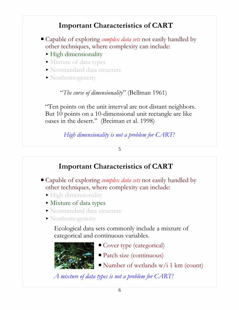
5
Important Characteristics of CART
“The curse of dimensionality” (Bellman 1961)
“Ten points on the unit interval are not distant neighbors.But 10 points on a 10-dimensional unit rectangle are likeoases in the desert.” (Breiman et al. 1998)
High dimensionality is not a problem for CART!
P Capable of exploring complex data sets not easily handled byother techniques, where complexity can include:< High dimensionality< Mixture of data types< Nonstandard data structure< Nonhomogeneity
6
Important Characteristics of CART
Ecological data sets commonly include a mixture ofcategorical and continuous variables.
A mixture of data types is not a problem for CART!
P Cover type (categorical)
P Patch size (continuous)
P Number of wetlands w/i 1 km (count)
P Capable of exploring complex data sets not easily handled byother techniques, where complexity can include:< High dimensionality< Mixture of data types< Nonstandard data structure< Nonhomogeneity
7
Important Characteristics of CART
Nonstandard data structure is not a problem for CART!
X1 X2 X3 X4 X5 X6
1 x x x x x x2 x x x x x x3 x x x x x x4 x x x x x x5 x x x x x x
X1 X2 X3 X4 X5 X6
1 x x x x x x2 x x x x3 x x x x4 x x x5 x x
Standard Structure Nonstandard Structure
P Capable of exploring complex data sets not easily handled byother techniques, where complexity can include:< High dimensionality< Mixture of data types< Nonstandard data structure< Nonhomogeneity
8
Important Characteristics of CART
Different relationshipshold between variablesin different parts of themeasurement space.
Nonhomogeneous data structure is not a problem for CART!
X1
X2
P Capable of exploring complex data sets not easily handled byother techniques, where complexity can include:< High dimensionality< Mixture of data types< Nonstandard data structure< Nonhomogeneity
9
01234567891011
-1 0 1 2 3 4 5 6 7 8 9 10a
Classification and Regression TreesGrowing Trees
10
red0.43
RedNode
Classification and Regression TreesGrowing Trees
01234567891011
-1 0 1 2 3 4 5 6 7 8 9 10a
11
Red
Split 1: a > 6.8
Blue
red0.55
a > 6.8
blue0.83
TerminalNode
Classification and Regression TreesGrowing Trees
01234567891011
-1 0 1 2 3 4 5 6 7 8 9 10a
12
Red
Split 1: a > 6.8
Blue
Split 2:b > 5.4
Green01234567891011
-1 0 1 2 3 4 5 6 7 8 9 10a
green0.69
red0.85
a > 6.8
b > 5.4blue0.83
Classification and Regression TreesGrowing Trees
red green blue
red 25 1 0
green 2 18 2
blue 2 0 10
13
Red
Split 1: a > 6.8
Blue
Split 2:b > 5.4
Green
a > 3.3
red0.89
green0.95
red0.85
a > 6.8
b > 5.4blue0.83
Split 3: a > 3.3
Red
Classification and Regression TreesGrowing Trees
01234567891011
-1 0 1 2 3 4 5 6 7 8 9 10a
14
Red
Split 1: a > 6.8
Blue
Split 2:b > 5.4
Green
a > 3.3
red0.89
green0.95
red0.85
a > 6.8
b > 5.4blue0.83
Split 3: a > 3.3
Red
Classification and Regression TreesGrowing Trees
01234567891011
-1 0 1 2 3 4 5 6 7 8 9 10a
Correct classification rate = 88%
red green blue
red 25 1 0
green 2 18 2
blue 2 0 10
15
1.At each node, the tree algorithmsearches through the variables oneby one, beginning with x1 andcontinuing up to xM.
2.For each variable, find best split.
3.Then it compares the M best single-variable splits and selects the best ofthe best.
4.Recursively partition each node untildeclared terminal.
5.Assign each terminal node to a class.
Classification and Regression TreesGrowing Trees
a > 3.3
red0.89
green0.95
red0.85
a > 6.8
b > 5.4blue0.83
Correct classification rate = 88%
16
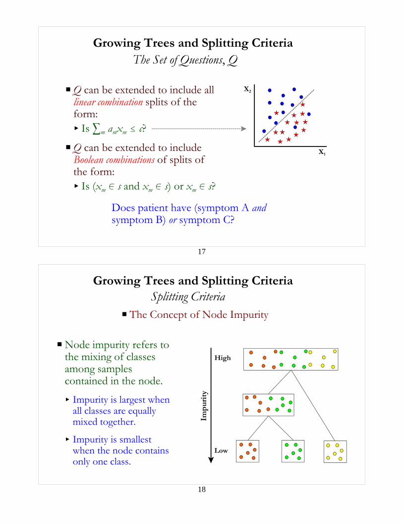
Growing Trees and Splitting Criteria
P Each split depends on the value of only a singlevariable (but see below).
P For each continuous variable xm, Q includes allquestions of the form:< Is xm # cn?< Where the cn are taken halfway between
consecutive distinct values of xm
P If xm is categorical, taking values {b1, b2, ..., bL},then Q includes all questions of the form:< Is xm 0 s?< As s ranges over all subsets of {b1, b2, ..., bL}
The Set of Questions, Q
Is patch size # 3 ha?
Is cover type = A?
17
Growing Trees and Splitting Criteria
P Q can be extended to include alllinear combination splits of theform:< Is 3m amxm # c?
P Q can be extended to includeBoolean combinations of splits ofthe form:< Is (xm 0 s and xm 0 s) or xm 0 s?
Does patient have (symptom A andsymptom B) or symptom C?
X1
X2
The Set of Questions, Q
18
Growing Trees and Splitting Criteria
P The Concept of Node Impurity
Splitting Criteria
P Node impurity refers tothe mixing of classesamong samplescontained in the node.
< Impurity is largest whenall classes are equallymixed together.
< Impurity is smallestwhen the node containsonly one class.
High
Low
i t p j t p j t( ) ( ) ln ( )
i t p j t( ) ( ) 1 2
i s t i t p i t p i tL L R R( , ) ( ) ( ) ( )
19
P Information Index:
P Gini Index:
P Twoing Index:At every node, select the conglomeration of classes into twosuperclasses so that considered as a two-class problem, thegreatest decrease in node impurity is realized.
p(j/t) = probability that a caseis in class j given that itfalls into node t; equalto the proportion ofcases at node t in class jif priors are equal toclass sizes.
Growing Trees and Splitting CriteriaSplitting Criteria
20
P At each node t, for each question in the set Q, thedecrease in overall tree impurity is calculated as:
i(t) = parent node impurity
pL,pR = proportion of observationsanswering ‘yes’ (descendingto left node) and ‘no’(descending to right node),respectively
i(tL,R) = descendent node impurity
Growing Trees and Splitting CriteriaSplitting Criteria
a > 3.3
red0.89
green0.95
red0.85
a > 6.8
b > 5.4blue0.83
Max i s t ( , )
i t p j t( ) ( ) 1 2
i s t i t p i t p i tL L R R( , ) ( ) ( ) ( )
Max i s t ( , )
21
P At each node t, select the split from the set Q thatmaximizes the reduction in overall tree impurity.
P Results are generally insensitive tothe choice of splitting index,although the Gini index isgenerally preferred.
P Where they differ, the Gini tendsto favor a split into one small,pure node and a large, impurenode; twoing favors splits that tendto equalize populations in the twodescendent nodes.
a > 3.3
red0.89
green0.95
red0.85
a > 6.8
b > 5.4blue0.83
Growing Trees and Splitting CriteriaSplitting Criteria
22
P Gini Index:
Growing Trees and Splitting Criteria
26 (.43)22 (.37)12 (.20)
12 48
0 (.00)2 (.17)10 (.83)
26 (.54)20 (.42)2 (.04)
i(t) =.638
Q1: a > 6.8
i(t) = .282 i(t) = .532
ªi(s,1) = .638 - (.2*.282) - (.8*.532) = .156
26 (.43)22 (.37)12 (.20)
24 36
16 (.67)0 (.00)8 (.33)
10 (.28)22 (.61)4 (.11)
i(t) =.638
Q2: b > 5.4
i(t) = .442 i(t) = .537
ªi(s,1) = .638 - (.4*.442) - (.6*.537) = .139
Best!
Red Blue
Green0
1
2
3
4
5
6
7
8
9
10
11
-1 0 1 2 3 4 5 6 7 8 9 10
a
r t p j t( ) max ( ) 1
R T r t p tt T
( ) ( ) ( )
max ( )p j t
( )j
p j t jN t
Nj
j( , ) ( )
( )
p j t p j tp j t
j
( ) ( , )( , )
23
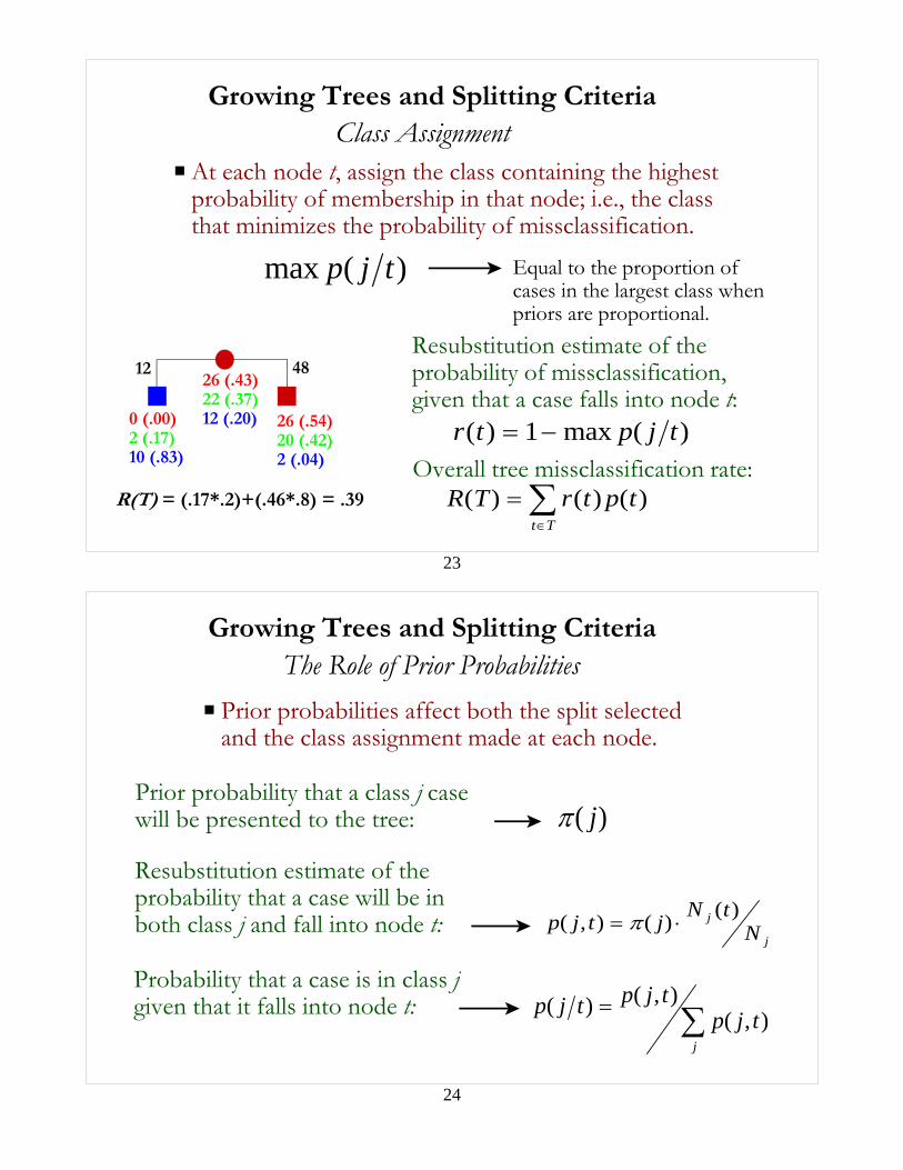
P At each node t, assign the class containing the highestprobability of membership in that node; i.e., the classthat minimizes the probability of missclassification.
Growing Trees and Splitting CriteriaClass Assignment
Resubstitution estimate of theprobability of missclassification,given that a case falls into node t:
Overall tree missclassification rate:
Equal to the proportion ofcases in the largest class whenpriors are proportional.
26 (.43)22 (.37)12 (.20)
12 48
0 (.00)2 (.17)10 (.83)
26 (.54)20 (.42)2 (.04)
R(T) = (.17*.2)+(.46*.8) = .39
24
P Prior probabilities affect both the split selectedand the class assignment made at each node.
Growing Trees and Splitting Criteria
Prior probability that a class j casewill be presented to the tree:
Probability that a case is in class jgiven that it falls into node t:
Resubstitution estimate of theprobability that a case will be inboth class j and fall into node t:
The Role of Prior Probabilities
( )jN
Nj
p j tN t
Nj( , )( )
p j tN t
N tj( )( )
( )
i t p j t( ) ( ) 1 2
i t p j t( ) ( ) 1 2
p j t jN t
Nj
j( , ) ( )
( )
( )j
p j t p j tp j t
j
( ) ( , )( , )
25
P Gini Splitting Index:
Growing Trees and Splitting Criteria
When priors match classproportions in sample:
Probability that a case is in class jgiven that it falls into node t:
Resubstitution estimate of theprobability that a case will be inboth class j and fall into node t:
Relative proportions of class j cases in node t
The Role of Prior Probabilities
26
P Gini Splitting Index:
Growing Trees and Splitting Criteria
When priors are userspecified:
Probability that a case is in class jgiven that it falls into node t:
Resubstitution estimate of theprobability that a case will be inboth class j and fall into node t:
The Role of Prior Probabilities
max ( )p j t
( )jN
Nj
p j tN t
Nj( , )( )
p j tN t
N tj( )( )
( )
p j t jN t
Nj
j( , ) ( )
( )
( )j
p j t p j tp j t
j
( ) ( , )( , )
max ( )p j t
27
P Class Assignment:
Growing Trees and Splitting Criteria
When priors match classproportions in sample:
Probability that a case is in class jgiven that it falls into node t:
Resubstitution estimate of theprobability that a case will be inboth class j and fall into node t:
Relative proportions of class j cases in node t
The Role of Prior Probabilities
28
P Class Assignment:
Growing Trees and Splitting Criteria
When priors are userspecified:
Probability that a case is in class jgiven that it falls into node t:
Resubstitution estimate of theprobability that a case will be inboth class j and fall into node t:
The Role of Prior Probabilities
29
Growing Trees and Splitting Criteria
0
1
2
3
4
5
6
7
8
9
10
11
-1 0 1 2 3 4 5 6 7 8 9 10
a
Red Blue Red Blue Red BluePriors: .75 .25 .50 .50 .20 .80
Node 2:# 9 8 9 8 9 8cp(j|2) .471 .529 .941 .529 5.647 .529S-Gini .498 .747 3.239Class Red Blue Blue
Node 3:# 21 2 21 2 21 2cp(j|3) .086 .913 .174 .913 1.043 .913S-Gini .159 .238 1.032Class Red Red Blue
Adjusting Missclassification Costs
0
1
2
3
4
5
6
7
8
9
10
11
-1 0 1 2 3 4 5 6 7 8 9 10
a
30 (.75)10 (.25)
17 23
9 (.53)8 (.47)
21 (.91)2 (.09)
Q1: a > 6.5
36
Growing Trees and Splitting CriteriaKey Points Regarding Priors and Costs
P Priors represent the probability of a class j case beingsubmitted to the tree.
< Increasing prior probability of class j increases therelative importance of class j in defining the best splitat each node and increases the probability of classassignment at terminal nodes (i.e., reduces class jmissclassifications.
– Priors proportional = max overall tree correctclassification rate
– Priors equal = max(?) mean class correctclassification rate (strives to achieve better balanceamong classes)
37
P Costs represent the ‘cost’ of missclassifying a class jcase.
< Increasing cost of class j increases the relativeimportance of class j in defining the best split at eachnode and increases the probability of classassignment at terminal nodes (i.e., reduces class jmissclassifications).
– Asymmetric but constant costs = can use GiniIndex with altered priors (but see below)
– Symmetric and nonconstant = use Symmetric GiniIndex (i.e., incorporate costs directly)
Growing Trees and Splitting CriteriaKey Points Regarding Priors and Costs
38
There are two ways to adjust splittingdecisions and final class assignmentsto favor one class over another.
Should I alter Priors or adjust Costs?
P My preference is to adjust priors to reflectinherent property of the population beingsampled (if relative sample sizes don’trepresent priors, then null approach is toassume equal priors).
P Adjust costs to reflect decisions regardingthe intended use of the classificationtree.
Growing Trees and Splitting CriteriaKey Points Regarding Priors and Costs
Characteristic Potential Preferred
Misclassification cost ratio (nest:random) 3:1 1:1
Correct classification rate of nests (%) 100 83
Total area (ha) 7355 2649
Area protected (ha) 5314 2266
Area protected (%) 72 86
Classification Tree
39
Growing Trees and Splitting CriteriaHarrier Example of Setting Priors and Costs
P 128 nests; 1000 randomP equal priorsP equal costs
P The most significant issue in CART is not growingthe tree, but deciding when to stop growing the treeor, alternatively, deciding on the right size tree.
Selecting the Right-Sized Trees
P Yet, overgrown trees do notproduce “honest” missclassificationrates when applied to new data.
P Missclassification rate decreases as thenumber of terminal nodes increases.
P The more you split, the better you thinkyou are doing.
The crux of the problem:
42
P The solution is to overgrow the tree and then pruneit back to a smaller tree that has the minimum honestestimate of true (prediction) error.
Selecting the Right-Sized TreesMinimum Cost-Complexity Pruning
P The preferred method is based on minimumcost-complexity pruning in combination with V-fold cross-validation.
R T R T T ( ) ( ) | |~
R T( )
| |~
T | |
~
T
R T( )
43
Cost-complexitymeasure:
Overall missclassification cost
Complexity parameter (complexitycost per terminal node)
Classification and Regression TreesIllustrated Example
52
P For a numeric explanatory variable (continuousor count), only its rank order determines a split. Trees are thus invariant to monotonictransformations of such variables.
Other CART IssuesTransformations
M x I s tm mt T
( ) (~ , )
~sm
53
P Cases with missing explanatory variables can behandled through the use of surrogate splits.
Other CART IssuesSurrogate Splits and Missing Data
1.Define a measure of similarity between any two splits,s, s’ of a node t.
2.If the best split of t is the split s on the variable xm, findthe split s’ on the variables other than xm that is mostsimilar to s.
3.Call s’ the best surrogate for s.
4.Similarly, define the second best surrogate split, thirdbest, and so on.
5.If a case has xm missing, decide whether it goes to tL ortR by using the best available surrogate split.
54
P How to assess the overall importance of avariable, despite whether or not it occurs in anysplit in the final tree structure?
Other CART IssuesSurrogate Splits and Variable Importance
Variable Ranking:
A variable can be ‘masked’ by another variablethat is slightly better at each split.
The measure ofimportance of variablexm is defined as:
= surrogate split on xm at node tWhere:
100M xM x
m
m m
( )max ( )
55
P Since only the relative magnitude of the M(xm) areinteresting, the actual measures of importance aregenerally given as the normalized quantiles:
x1 x2 x3 x4 x5 x6 x7 x8 x9
100%
0%
Variables
Other CART IssuesSurrogate Splits and Variable Importance
Variable Ranking:
*Caution, the size of the treeand the number of surrogatesplitters considered will affectvariable importance!
56
P At any given node, there may be a number of splits ondifferent variables, all of which give almost the same decreasein impurity. Since data are noisy, the choice between competingsplits is almost random. However, choosing an alternative splitthat is almost as good will lead to a different evolution of thetree from that node downward.
< For each split, we can compare the strength of the split dueto the selected variable with the best splits of each of theremaining variables.
< A strongly competing alternative variable can be substitutedfor the original variable, and this can sometimes simplify atree by reducing the number of explanatory variables or leadto a better tree.
Other CART IssuesCompeting Splits and Alternative Structures
57
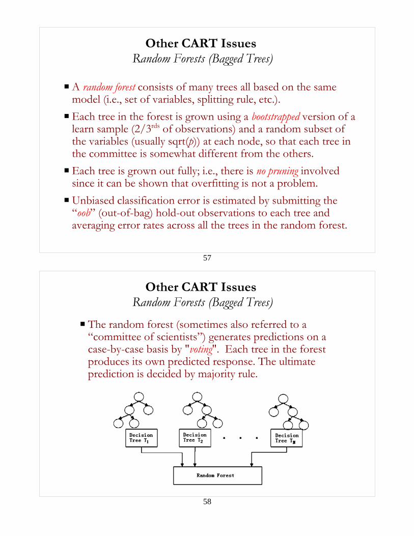
Other CART IssuesRandom Forests (Bagged Trees)
P A random forest consists of many trees all based on the samemodel (i.e., set of variables, splitting rule, etc.).
P Each tree in the forest is grown using a bootstrapped version of alearn sample (2/3rds of observations) and a random subset ofthe variables (usually sqrt(p)) at each node, so that each tree inthe committee is somewhat different from the others.
P Each tree is grown out fully; i.e., there is no pruning involvedsince it can be shown that overfitting is not a problem.
P Unbiased classification error is estimated by submitting the“oob” (out-of-bag) hold-out observations to each tree andaveraging error rates across all the trees in the random forest.
58
P The random forest (sometimes also referred to a“committee of scientists”) generates predictions on acase-by-case basis by "voting". Each tree in the forestproduces its own predicted response. The ultimateprediction is decided by majority rule.
Other CART IssuesRandom Forests (Bagged Trees)
59
Other CART IssuesRandom Forests (Bagged Trees)
P Variable Importance:
1) Mean decrease in accuracy =For each tree, theprediction error on the oobportion of the data isrecorded. Then the same isdone after permuting eachpredictor variable. Thedifference between the twoare then averaged over alltrees, and normalized by thestandard deviation of thedifferences.
60
Other CART IssuesRandom Forests (Bagged Trees)
P Variable Importance:
2) Mean decrease in Gini =total decrease in nodeimpurities from splitting onthe variable, averaged overall trees.
61
Other CART IssuesRandom Forests (Bagged Trees)
P Variable Importance:
62
Other CART IssuesRandom Forests (Bagged Trees)
P Proximity:
Measure of proximity (orsimilarity) based on how oftenany two (oob) observationsend up in the same terminalnode. 1-prox(k,n) formEuclidean distances in a highdimensional space that can beprojected down onto a lowdimensional space using metricscaling (aka principalcoordinates analysis) to give aninformative view of the data.
63
Other CART IssuesRandom Forests (Bagged Trees)
P Variable Importance:
2) Mean decrease in Gini =total decrease in nodeimpurities from splitting onthe variable, averaged overall trees.
64
Other CART IssuesBoosted Classification & Regression Trees
P Boosting involves growing a sequence of trees, with successivetrees grown on reweighted versions of the data. At each stage ofthe sequence, each data case is classified from the current sequenceof trees, and these classifications are used as weights for fitting thenext tree of the sequence. Incorrectly classified cases receive moreweight than those that are correctly classified, and thus cases thatare difficult to classify receive ever-increasing weight, thereby increasing their chance of being correctly classified. The final classification of each case is determined by the weighted majority of classifications across the sequence of trees.
a x ck kk
K
1
65
Limitations of CART
P CART’s greedy algorithm approach in which all possiblesubsets of the data are evaluated to find the “best” splitat each node has two problems:
< Computational Complexity...the number of possiblesplits and subsequent node impurity calculations canbe computionally challenging.
< Bias in Variable Selection...
P Ordered variable:
P Categorical variable:
P Linear combinations ofordered variables:
#splits = n-1 n = #distinct values
#splits = 2 (m -1) -1 m = #classes
#splits = {a1,...aK,c}
66
Limitations of CART
P CART’s greedy algorithm approach in which all possiblesubsets of the data are evaluated to find the “best” split ateach node has two problems:
< Computational Complexity...
< Bias in Variable Selection...unrestricted search tends toselect variables that have more splits, making it hard todraw reliable conclusions from the tree structures
P Alternative approaches exist (QUEST) in which variableselection and split point selection are done separately. Ateach node, an ANOVA F-statistic is calculated (after a DAtransformation of categorical variables) and the variable withthe largest F-statistic is selected, and then quadratic two-group DA is applied to find the best split (if >2 groups, then2-group NHC is used to create 2 superclasses).
67
Caveats on CART
P CART is a nonparametric procedure, meaning that it isnot based on an underlying theoretical model, incontrast to Discriminant Analysis, which is based on alinear response model, and Logistic Regression which isbased on a logistic (logit) response model.
What are the implications of this?
P Lack of theoretical underpinning precludesan explicit test of ecological theory?
P Yet the use of an empirical model means thatour inspection of the data structure is notconstrained by the assumptions of aparticular theoretical model?
68
P Are groups significantly different? (How validare the groups?)< Multivariate Analysis of Variance (MANOVA)< Multi-Response Permutation Procedures (MRPP)< Analysis of Group Similarities (ANOSIM)< Mantel’s Test (MANTEL)
P How do groups differ? (Which variables bestdistinguish among the groups?)< Discriminant Analysis (DA)< Classification and Regression Trees (CART)< Logistic Regression (LR)< Indicator Species Analysis (ISA)
Discrimination Among Groups
p ke
e
b b x b x b x
b b x b x b x
k k m km
k k m km
0 1 1 2 2
0 1 1 2 21
...
...
ln ...p k
p kb b x b x b xk k m km1 0 1 1 2 2
69
Logistic Regression
P Parametric procedure useful for exploration,description, and prediction of grouped data(Hosmer and Lemenshow 2000).
P In the simplest case of 2 groupsand a single predictor variable,LR predicts groupmembership as a sigmoidalprbabilistic function for whichthe prediction ‘switches’ fromone group to the other at acritical value, typically at theinflection point or value whereP[y=1] = 0.5, but it can bespecified otherwise.
Predictor variable x
1.0
0.0
70
Logistic Regression
P Logistic Regression can be generalized to includeseveral predictor variables and multiple (multinomial)categorical states or groups.
P Exponent term is aregression equationthat specifies a logit (logof the odds) modelwhich is a likelihoodratio that contrasts theprobability ofmembership in onegroup to that ofanother group.
xn
xjk
kijk
i
nk
1
1
RA x
xjk
jk
jk
k
g
1
RFb
njk
ijki
n
k
k
1
71
Logistic Regression
P Can be applied to any data structure, including mixed datasets containing both continuous, categorical, and countvariables, but requires standard data structures.
P Like DA, cannot handle missing data.
P Final classification has a simple form which can becompactly stored and that efficiently classifies new data.
P Can be approached from a model-selection standpoint,using goodness-of-fit tests or cost complexity measures(AIC) to choose the simplest model that fits the data.
P Regression coefficients offer the same interpretive aid as inother regression-based analyses.
72
Indicator Species AnalysisP Nonparametric procedure for distinguishing among groups
based on species compositional data, where the goal is toidentify those species that show high fidelity to aparticular group and as such can serve as indicators forthat group (Dufrene and Legendre 1997).
P Compute the mean within-groupabundance of each species j ineach group k.
P Compute an index of relativeabundance within each group.
P Compute an index of relativefrequency within each group basedon presence/absence data.
IV RA RFjk jk jk 100( )
RELATIVE ABUNDANCE in group, % of perfect indication (averageabundance of a given species in a given group over the averageabundance of that species groups expressed as a %) Group Sequence: 1 2 3 4 Identifier: 1 2 3 4 Number of items: 71 36 52 5 Column Avg Max MaxGrp 1 AMGO 25 97 4 0 1 2 97 2 AMRO 25 64 4 3 17 16 64 3 BAEA 25 100 3 0 0 100 0 4 BCCH 25 84 4 0 5 10 84 5 BEKI 25 63 3 0 37 63 0 6 BEWR 25 78 4 1 0 21 78 7 BGWA 25 95 3 5 0 95 0 8 BHGR 25 39 4 4 27 29 39 9 BRCR 25 78 2 12 78 10 0 Averages 24 70 6 20 36 35
RELATIVE FREQUENCY in group, % of perfect indication(% of plots in given group where given species is present) Group Sequence: 1 2 3 4 Identifier: 1 2 3 4 Number of items: 71 36 52 5 Column Avg Max MaxGrp 1 AMGO 28 100 4 0 3 8 100 2 AMRO 62 100 4 18 64 67 100 3 BAEA 0 2 3 0 0 2 0 4 BCCH 34 100 4 1 11 25 100 5 BEKI 4 10 3 0 6 10 0 6 BEWR 21 60 4 1 0 23 60 7 BGWA 5 19 3 1 0 19 0 8 BHGR 75 100 4 28 81 90 100 9 BRCR 24 64 2 18 64 15 0 Averages 24 49 12 22 26 37
RELATIVE ABUNDANCE in group, % of perfect indication (average
73
Indicator Species Analysis
P Compute indicator values foreach species in each group.
P Each species is assigned as anindicator to the group forwhich it receives its highestindicator value.
P Indicator values are tested forstatistical significance by MonteCarlo permutations of thegroup membershipassignments.
MONTE CARLO test of significance of observed maximum indicatorvalue for species 1000 permutations.------------------------------------------- IV from Observed randomized Indicator groups Column Value (IV) Mean S.Dev p * ------------- -------- ----- ------ ------- 1 AMGO 97.3 6.6 4.60 0.0010 2 AMRO 64.5 19.7 6.48 0.0010 3 BAEA 1.9 2.3 2.77 0.5350 4 BCCH 83.8 10.0 5.92 0.0010 5 BEKI 6.1 6.1 4.97 0.3180 6 BEWR 46.7 8.5 5.37 0.0020 7 BGWA 18.2 7.3 5.13 0.0360 8 BHGR 39.2 23.0 5.62 0.0260 9 BRCR 49.6 13.6 5.49 0.0010-------------------------------------------* proportion of randomized trials with indicator value equal to or exceeding the observed indicator value.