DISCUSSION PAPER PI-1408 The Market for Lemmings: The Herding Behavior of Pension Funds David Blake, Lucio Sarno, and Gabriele Zinna December 2016 ISSN 1367-580X The Pensions Institute Cass Business School City University London 106 Bunhill Row London EC1Y 8TZ UNITED KINGDOM http://www.pensions-institute.org/
Transcript
DISCUSSION PAPER PI-1408 The Market for Lemmings: The Herding Behavior of Pension Funds David Blake, Lucio Sarno, and Gabriele Zinna December 2016
ISSN 1367-580X The Pensions Institute Cass Business School City University London 106 Bunhill Row London EC1Y 8TZ UNITED KINGDOM http://www.pensions-institute.org/
∗We are indebted for their constructive comments to Tarun Chordia (Co-Editor), an anonymous referee,Tamara Li, Taneli Makinen, George Pennacchi, Alberto Rossi and Allan Timmermann. We are particularlyindebted to Andrew Haldane and the other members of the Procyclicality Working Group of the Bank of Englandfor their extensive comments and for supporting some of this research. We would also like to thank AlastairMacDougall at State Street Investment Analytics for his help in providing us with the dataset used in this studyand for his valuable comments. This research was started when Gabriele Zinna was working at the Bank ofEngland, and was partly carried out while Lucio Sarno was Visiting Professor at the Cambridge Endowmentfor Research in Finance (CERF) of the University of Cambridge and the Einaudi Institute for Economics andFinance (EIEF). All errors are our responsibility. The views expressed in this paper are those of the authors anddo not necessarily reflect those of the Bank of England or the Bank of Italy.†Cass Business School, City University of London, London. E-mail: [email protected]‡Cass Business School, City University of London, London, and Centre for Economic Policy Research (CEPR).
‘Institutions are herding animals. We watch the same indicators and listen to the
same prognostications. Like lemmings, we tend to move in the same direction at the
same time.’
Wall Street Journal, October 17, 1989
At least since the early 1990s, a number of studies have suggested that institutions are more
likely to herd than individual investors. A recurrent argument, for example, is that institutional
investors know more about each other’s trades than do individual investors (Banerjee, 1992;
Bikhchandani, Hirshleifer and Welch, 1992) and react to the same exogenous signals (Froot,
Scharfstein and Stein, 1992). Also, the signals that reach institutions are generally more highly
correlated than those that reach individuals (Lakonishok, Schleifer and Vishny, hereafter LSV,
1992). This increases the likelihood that institutional investors herd more than individual
investors. In addition, fear of relative underperformance compared with the peer group of
investment managers creates an explicit incentive for these managers to herd (Shleifer, 1985;
Scharfstein and Stein, 1990).
Institutional herds are of particular interest as they can potentially impact the dynamics
of asset prices (e.g., Chan and Lakonishok, 1995; Dennis and Strickland, 2002), and impose
severe externalities on financial markets (e.g., Stein, 2009). For reasons of data availability,
thus far the empirical literature has largely focused on mutual funds (e.g., Grinblatt, Titman
and Wermers, 1995; Wermers, 1999; Coval and Stafford, 2007), and more recently on leveraged
investors such as hedge funds (e.g., Reca, Sias, and Turtle, 2014). In contrast, relatively little
is known about the investment behavior of pension funds. Yet, they constitute an increasingly
large class of institutional investors and operate in an institutional setting which, particularly
in recent years, imposes a set of constraints on their investment decisions (Domanski, Shin and
Sushko, 2015). In turn, this not only makes their demands for assets highly inelastic, it might
also induce a tendency for pension funds to herd.1
LSV (1992) produced one of the few studies to examine herding in the pension fund industry.
They conclude that there is no evidence for herding in pension funds investment behavior, which
1Some recent studies argue that portfolio rebalancing and hedging activities by large institutional investors,such as pension funds, can eventually result in positive feedback loops, and can therefore pose severe risks for thestability of financial markets (e.g., Haldane, 2014; Domanski, Shin and Sushko, 2015). For example, Malkhozov,Mueller, Vedolin and Venter (2015) show, both theoretically and empirically, that the hedging activity of investorsin the US mortgage-backed securities market (i.e., which leads to their asset demands being highly inelastic)amplifies movements in long-term rates.
1
is perhaps surprising, since this differs from the experience of many other types of institutional
investors. However, the conclusion of LSV (1992) is subject to the important caveat that:
‘while there is very little herding in individual stocks and industries, there are times when
money managers simultaneously move into stocks as a whole or move out of stocks as a whole.
Since our dataset contains only all-equity funds, we cannot examine this type of herding’ (LSV,
1992, p. 35). LSV also conjecture that, due to the structure of the pension fund industry,
herding might be more prevalent among subgroups of pension funds rather than in aggregate,
but their data did not allow them to test this interesting conjecture.
The primary goal of this paper is to address these issues in order to refine our understand-
ing of the investment behavior of pension funds. First, we focus on pension fund herding in
asset classes rather than in individual stocks. Second, we investigate whether herding is more
predominant in subgroups; we classify pension funds into subgroups according to their size and
sponsor type. Our analysis is made possible thanks to a unique dataset that covers UK private-
sector and public-sector defined benefit (DB) pension funds’ monthly asset allocations over the
past 25 years. We have information on the funds’ total portfolios and asset class holdings, and
are also able to decompose changes in portfolio weights into valuation effects and flow effects.2
The empirical analysis establishes three sets of results about the herding behavior of pension
funds. First, we address the question of whether pension funds herd, and our results provide
robust evidence of herding in the asset allocations of pension funds. In particular, we document a
positive relationship between the cross-sectional variation in pension funds’ net asset demands
in a given month and their net demands in the preceding month, providing support for the
hypothesis that pension funds herd together in the very short term. These results are obtained
using the test proposed by Sias (2004) and also confirmed using the original test of LSV (1992).
Second, we analyze how pension funds herd, and find strong evidence that pension funds
herd in subgroups. Private-sector pension funds follow other private-sector funds more than
public-sector funds, and public-sector funds follow other public-sector funds more than private-
sector funds. Similarly, we find that pension funds tend to follow other funds of similar fund
2There are very few studies on pension fund flows, possibly because of the difficulty in obtaining reliabledata until recently. Some examples are the papers of Sialm, Starks, and Zhang (2015a,b) which compare mutualfund flows of defined contribution plans with the fund flows of other mutual fund investors. Huberman andSengmueller (2004) examine retirement plans’ allocation of funds and transfers to or from company stocks. Ofparticular note for our study is Pennacchi and Rastad (2011), who show that career concerns often prevail over theoptimal strategy of public-sector pension funds to immunize the risk of their liabilities. In their study, the assetallocation chosen by trustees and their consultants is largely driven by the performance of peer-group pensionfunds.
2
size. We then examine the effect of sponsor type controlling for size. We do this by double
sorting funds by sponsor type (private-sector and public-sector) and by size (small, medium
and large), and we find that public-sector funds follow other public-sector funds of similar size,
while large private-sector funds strongly follow other large private-sector funds. Furthermore,
the empirical evidence allows us to rule out the possibility that pension fund herding is due
either to habit investing (i.e., serially correlated fund cash flows) or to momentum (i.e., positive
feedback) trading.
Our findings suggest that it is unlikely that pension funds herd because of superior informa-
funds. Two types of rebalancing are identified. First, there is mechanical rebalancing towards
their long-term asset mix which, in turn, is driven by their liability. Although we do not have
data on the pension funds’ liabilities, we can draw inferences about the changing maturity of
their liabilities from the longer-term dynamic asset allocation strategies pursued over the course
of the sample period. Most private-sector plans have closed both to new members and to fu-
ture accrual by existing members, whereas public-sector plans are still open. This implies that
private-sector plans are more mature than public-sector plans of similar size. We document
that, as the maturity of their liabilities has increased, private-sector pension funds have sys-
tematically switched from equities to conventional and index-linked bonds in line with standard
asset-liability management (ALM). The analysis also suggests that the average pension fund –
as represented by the peer-group benchmark – appears to choose the long-term asset mix which
matches its liability profile. Second, our findings also indicate strong short-term mechanical
portfolio rebalancing by pension funds, i.e., pension funds correct changes in portfolio weights
resulting from short-term valuation changes that drive the weights away from the asset mix
specified in their investment mandate.
Third, we investigate whether pension fund herding impacts asset prices, and uncover some
evidence that pension funds exert a price impact and provide short-term liquidity to financial
markets. However, we find that the price impact is not persistent. This, in turn, suggests that
pension fund trades are largely uninformed, in the sense of not reflecting changes in expected
returns, a finding that is largely consistent with our earlier results showing that pension funds
rebalance their portfolios in a mechanical fashion. In the long term, there are systematic changes
in the strategic asset allocation (SAA) of the average fund which reflect its changing liability
structure. So there is little room for the average fund to react to changes in the expected
3
returns and risks on the assets (which are the signals to which informed active managers would
respond). Our results indicate that pension funds’ investment behavior does not help move asset
prices towards their fundamental values and, therefore, does not play a strongly stabilizing role
on financial markets.
Finally, we examine pension funds’ performance, and provide evidence that there are only
small cross-sectional differences in returns across pension funds, consistent with widespread
herding behavior by UK pension funds. We also document that the best performing funds are
private and large. These funds tend to herd less, and follow more their own trades, than the
other funds. Conversely, the worst performing funds tend to be small and have higher weightings
in bonds relative to equities - a feature that is consistent with these funds being more mature.
To conclude the analysis, we investigate the market exposure of the average pension fund
in our sample and find that the peer-group benchmark returns match very closely the returns
on the relevant external asset-class market index. This result, coupled with the evidence on
herding, supports anecdotal evidence that pension funds herd around the average fund which
generates the peer-group average return and who is, in turn, no more than a ‘closet index
matcher’.3
The rest of the paper is organized as follows. Section 2 discusses the institutional features
of the pension fund industry in the UK, and Section 3 describes our data in detail. Section
4 provides the core empirical results on pension funds’ herding; we examine whether and why
pension funds herd, and whether their herding activity exerts a price impact. Section 5.1 sheds
light on some aspects of pension funds’ performance. Finally, Section 6 concludes the paper.
Further details are provided in the Appendix, and a number of extensions and robustness checks
are reported in the Internet Appendix.
2 The UK Pension Fund Industry: Institutional Details
In this section, we first review the main regulatory and accounting reforms, which led UK pen-
sion funds to use liability-driven investment (LDI) strategies. Then, we describe the governance
of UK DB pension funds. This description of the industry suggests naturally the possibility
that pension funds follow other pension funds with similar characteristics into and out of the
3‘Closet indexing’ refers to the practice of some so-called ‘active funds’ having weights that differ very littlefrom those underlying the benchmark index. A recent study by Cremers, Ferreira, Matos and Starks (2015) findsthat closet indexing is common in the mutual fund industry.
4
same asset classes, i.e. they herd in subgroups.
Prior to the mid-1990s, UK pension funds were able to optimize the risk-return profile of their
assets, since their liabilities were ‘immature’ and so could be disregarded when it came to setting
the funds’ investment strategy. Furthermore, for most of its history, the UK pensions industry
was subject to a light-touch regulatory framework with little need for accounting transparency.
After the mid-1990s, however, not only did the maturity of pension funds increase, but also
a range of regulatory and accounting changes – the Pension Acts of 1995 and 2004, the 1997
Minimum Funding Requirement, and the 2000 Financial Reporting Standard 17 (which was
superseded by the International Accounting Standard 19) – were introduced aimed at enhancing
the resilience and transparency of the UK pension fund industry (Blake, 2003; Greenwood and
Vayanos, 2010). All these changes had a strong influence on pension funds’ ALM strategies,
linking SAA much more closely to the development of plan liabilities. Pension funds became
more likely to follow LDI strategies, reducing their historically high weight in equities and
replacing these with conventional and inflation-linked government bonds, together with interest
rate and inflation swaps.
The pension funds in our dataset invest the accruing contributions of DB pension plans.
The pension plans have sponsors, namely the employers that established the plans for their
retired employees, and the security of the pensions promised (i.e., the liabilities) depends on the
assets backing the liabilities plus (in the case of plans in deficit where the value of the assets
is less than the value of the liabilities) the strength of the sponsor covenant to make good the
deficit over time. Standing between the sponsor and the plan beneficiaries are the plan trustees
or fiduciaries. The trustees are nominated by the sponsor and a minority can be nominated
by the beneficiaries, but they have a legal duty to act in the interests of the beneficiaries. In
exercising this duty, they are advised by consultants, since most trustees are part-time and often
do not have much investment or actuarial expertise. The consultants advise the trustees on the
value of the liabilities and the strength of the sponsor covenant. They also advise trustees on
the funding strategy needed to remove any deficit over an agreed period and the investment
strategy.
The investment strategy has two components. The first is the SAA: the broad mix of asset
classes intended to match the maturity profile of the liabilities. A young immature pension plan
will invest heavily in equities and other growth assets. Then, as the plan matures, the SAA
will switch to bonds and bond-like assets which have the stable cash flows needed to deliver the
5
pensions in retirement.4 This is generally regarded as the passive component of the investment
strategy. The second component is the active component, i.e., the strategy of trading in and
out of different asset classes and securities with the aim of generating additional returns beyond
a passive strategy in order to reduce the sponsor’s funding costs.
There are other institutional features of the UK pension fund industry which are important
to the understanding of pension funds’ investment behavior, and their tendency to herd in
subgroups. First, the consultant will advise the trustees on both the SAA and the appointment
of the investment managers. The consultant will typically express the SAA in terms of a
benchmark comprising the main asset classes with weights that reflect the plan’s maturity.
The investment managers will be given an investment mandate that specifies their investment
objectives. In particular, the mandate may contain a performance benchmark which, although
is usually tailored to the circumstances of the fund, might also make reference to the investment
manager’s peer group.5 As a result, trustees in different plans, but with similar characteristics,
are likely to be given similar advice at the same time. This is also because consultants tend
to specialize in funds of similar types, and the UK consultancy industry is much more heavily
concentrated than in other parts of the world.6 Thus, the advice that reaches pensions funds is
highly correlated across funds of similar types, and this might induce pension funds to implement
similar trades.
Second, managers can deviate from the SAA benchmark when they attempt to generate
additional returns from the active strategies of security selection and market timing. However,
there are limits to their investment freedom expressed in terms of a risk budget, which sets out
how far they can depart from the benchmark. If the funds violate their risk budget, then they
will mechanically rebalance their portfolios. The fund’s risk budget, in turn, depends on the
funding position and the strength of the sponsor covenant. Thus, investment managers in plans
that are well funded with a strong sponsor will have a larger risk budget than those in plans
4As funds mature, they would be expected to move away from equities and into bonds, regardless of theirfunding status and sponsor covenant strength (Sundaresan and Zapatero, 1997; Lucas and Zeldes, 2009; Benzoni,Collin-Dufresne and Goldstein, 2007; Andonov, Bauer and Cremers, 2013).
5For example, the investment manager might be set the task of being in the first quartile of peer groupperformance over a specified horizon.
6In particular, the UK pension fund industry is much more concentrated than the US industry. LSV (1992)document that none of the independent investment counselors in the US pension group had a market sharelarger than 4 percent. In contrast, there are three large consultants in the UK and, in 1993, five fund managersaccounted for about 80 percent of the market (Blake, Lehmann and Timmermann, 1999). The consultants advisea number of funds, many of which will be in similar positions in terms of funding ratios and maturity. Further,some consultants specialize in advising certain classes of pension fund, such as local authority (i.e., municipal)funds.
6
with a deficit and a weak sponsor. This implies that funds with similar risk budgets are likely
to rebalance their portfolios at a similar time.
Third, the consultants and trustees do not interfere with the day-to-day decisions taken
by the investment managers, but they will monitor their managers’ investment performance,
typically quarterly. The fear of underperforming the peer-group can, in turn, induce the fund
manager to follow the asset allocation of their peers.7 In addition, the high frequency of assess-
ment against a peer-group benchmark may limit the extent to which pension funds engage in
active management, which would also result in correlated trades among pension funds of similar
maturity.
Fourth, different pension funds may well hire the same investment manager. It is also
plausible that each investment manager will manage assets for different pension funds in a
similar fashion. However, it is important to note that pension funds’ mandates to investment
managers are asset-class specific. Therefore, while the fact that multiple pension funds may
be using the same investment manager which, in turn, can generate some form of herding
at the level of individual securities, this does not have obvious implications for herding at the
asset-class level. Indeed, as mentioned earlier, the decision on how to rebalance portfolios across
asset classes is made by pension funds on the basis of advice from consultants. Put another way,
investment managers receive mandates for discretionary asset management from pension funds
which are specific with respect to, among other things, the asset class and the plan sponsor’s
level of risk tolerance, but they have no influence on how pension funds set the SAA.8
Testable Implications. The above discussion suggests that we should not be surprised to
observe pension funds following each other into and out of the same asset classes, thus exhibiting
herding behavior. A careful examination of the institutional setting, however, suggests that this
herding is more likely to take place in subgroups. These subgroups should be defined in terms
of the funds’ maturity, investment mandates, risk budgets and choice of consultant.
Unfortunately we do not have data on these factors, but we conjecture that their impact
can be well captured by fund size and sponsor type (private vs public). As we have mentioned,
7Short-term under performance and the failure to fulfill the original mandate are often the reasons why fundmanagers are dismissed (Financial Times, 2014). More generally, relative performance is used as a marketingdevice through which active investment managers compete for clients.
8It is common for specialist investment managers to be appointed for each asset class, especially in large plans.It used to be common, especially at the beginning of the sample period, for balanced managers to be appointedto manage across all asset classes; for small schemes, this is still the case. However, the SAA for each pensionfund is still chosen by the consultant and the investment manager will be set a separate objective for each assetclass.
7
consultants tend to specialize by size and type of fund, and investment managers tend to be
assessed relative to funds of similar size and sponsor type. Furthermore, most of the private-
sector plans are closed, whereas all the public-sector plans are still open. This implies that
private-sector plans are likely to be more mature than public-sector plans of the same size.
This will have implications for the SAA. Public-sector funds may also have a stronger sponsor
covenant, as they benefit from an implicit government guarantee. The strength of the sponsor
covenant, however, tends also to increase with the size of the fund. Therefore, smaller funds,
particularly in the private sector, are likely to be associated with weaker sponsor covenants than
larger funds.
Overall, given the institutional setting of the pension fund industry described above, we are
interested in testing whether pension funds herd and how they herd, and in particular whether
they follow each other into and out of the same asset classes in subgroups defined by sponsor
type and fund size. Given the large size of pension funds, we are also interested in whether they
exert an impact on asset prices.
It is important to note here that our definition of herding is somewhat different from what
is typically considered herding in the literature. This is because pension funds might herd in
asset classes for a number of reasons that are unrelated to the discretionary decisions of indi-
vidual managers following their investment mandates, such as career concerns (e.g., managers’
fears of underperformance) and the nature of pension fund investing (e.g., LDI and portfolio
rebalancing). We consider this broader definition of herding because, although the reasons why
pension funds display correlated trades might differ, the consequences in terms of, say, price
impact are the same.
3 Data and Descriptive Statistics
The data used in this paper were provided to us by State Street Investment Analytics (SSIA
hereafter) and consist of monthly observations on 189 UK DB pension funds from January 1987
to December 2012.9 The data are in the form of an unbalanced panel, covering a total of 108
corporate and 81 local authority pension funds.10 For each fund, we have data on the overall
9The SSIA is one of the two key performance measurement services in the UK, the other is CAPS (CombinedActuarial Performance Services). The SSIA database was originally owned by the WM Company.
10In this study, the terms corporate funds and private-sector funds, and similarly local authority funds andpublic-sector funds, are used interchangeably. Within the UK public sector, only local authority (municipal)employees have funded pension plans.
8
portfolio (i.e., total assets) and the following seven constituents: equities (UK and international),
conventional bonds (UK and international), index-linked bonds (UK only), cash/alternatives,
and property. Cash/alternatives is a catch-all residual category that includes, e.g., investment
in both money market instruments and hedge funds; however, the investment in hedge funds is
largely concentrated in the second part of the sample. For each asset class and each month, every
fund reported initial market value, average fund value, dividend, return and net investment. We
also have information on peer-group benchmark returns and the returns on the external market
indices that SSIA uses in its analysis. The identities of the funds are unknown and we have
no direct information on their liabilities. However, the changing asset weights over the sample
period allow us to draw inferences about the development of the funds’ liabilities over time.
The dataset covers roughly one third by value of the UK pension fund industry as of 2012, and
about half of all funds operating in the UK over the sample. Figure 1 shows asset holdings over
the sample period by sponsor-type of pension fund, i.e., private-sector vs public-sector.
3.1 Pension Fund Returns and Asset Holdings
Table 1 presents summary statistics for the annualized monthly returns of the pension funds in
our sample for 1987-2012. During this period, equities generated the highest average return (9.4
percent) and cash/alternatives the lowest (5.6 percent). The strong performance of equities is
largely driven by the return on domestic rather than international equities. The median return
on equities is substantially larger than the average return, a consequence of the dramatic fall in
equity prices during the recent global financial crisis. The returns on both cash/alternatives and
property are highly autocorrelated. The average returns in each asset class are broadly similar
for both corporate and local authority pension funds, despite having substantially different asset
allocations.
Figure 2 shows that, for corporate pension funds, the equity weighting decreased significantly
from a peak of 79 percent in 1993 to 36 percent in 2012. Over the same period, their weighting in
index-linked bonds increased from 3 percent to 15 percent, while their allocation to conventional
bonds increased from 7 to 30 percent. The weightings to property diminished over the period. In
contrast, the portfolios of local authority funds display rather more gradual shifts in allocations
over the sample period, with their allocation to equities falling from 81 percent in 1993 to
62 percent in 2012. Their weighting in conventional and index-linked bonds were roughly 13
percent and 4 percent in 2012, respectively. The de-risking of corporates, which contrasts with
9
the high exposure to equities maintained by local authorities, is consistent with their differing
liability profiles. The plan closures in the private sector began in the late 1990s, first slowly and
then more rapidly during the first decade of this century. The effect of closure is to increase
rapidly the maturity of a pension fund’s liabilities (by reducing the duration of the pension
fund’s projected net cash outflows in the form of pension payments). The stronger sponsor
covenant in local authority plans, compared with corporate plans, arising from the taxation
powers of local authorities, enables them to take more risk.11
Changes in the asset mix of pension fund portfolios can result either from valuation or flow
(net investment) effects. Figure 3 presents the cumulative sum of both corporate and local
authority pension funds’ net investment in the various asset classes. There are two distinct
phases of net investment in equities, one of which peaks in 1992 and the other in 2004. Net
investment in conventional bonds has been substantial since 1994, except for the 2000-01 and
2008-09 stock market crashes. Purchases of inflation-linked bonds were particularly strong
during the 1991-97 and 2003-07 periods. The net investment in property has been fairly stable
for the whole period and especially during the 2008-12 period, although this has mainly been
by local authorities.
The government ended the tax relief that pension funds could claim on UK dividend pay-
ments in 1997 and this encouraged pension funds to switch out of UK equities into international
equities. By 2005, pension funds (in aggregate) held a larger fraction of international equities
than UK equities. Figure A1, in the on line appendix, shows very different net investment
behavior by private- and public-sector funds, mainly because of their different maturities. Cor-
porate funds began disinvesting from UK equities in 1998 and, although they switched into
international equities, growth in this category slowed significantly after 2004. In contrast, local
authority funds actually increased their holdings of UK equities after 1998 and only began to
disinvest after 2010; their net investment in international equities grew very rapidly starting
from 1998. The two fund types exhibit similar behavior when it comes to bonds, however, as
Figure A2, in the on line appendix, shows. Their allocations to UK conventional bonds began
to grow after 1995, to UK index-linked bonds after 1991, and to international bonds after 1989.
11Such risk taking behavior is also common in US public sector funds, which actually increased their investmentsin equities and alternatives from 57% to 73% between 1993 and 2010 (Cohen, 2014).
10
3.2 Peer-Group and External Benchmarks
The two main types of benchmarks used in the UK to evaluate pension fund performance
are external asset-class benchmarks and peer-group benchmarks. In the early 1970s, when
performance measurement started, most pension funds selected customized benchmarks which
were based on external indices with weights tailored to the specific objectives of the fund.
Interest in how other pension funds were performing quickly led to the introduction of peer-
group benchmarks. Since the mid-2000s, an increasing number of funds returned to customized
benchmarks to reflect the maturity profile of their liabilities. However, for most of our sample
period, peer-group benchmarks dominated.12 Even where a fund has a customized benchmark,
it is possible that this is set to equal the peer-group benchmark, as long as the asset mix of the
latter approximately matches the fund’s specific circumstances (WM Company, 1997).
Each month, SSIA collects individual fund returns and weights, and aggregates them into
peer-group benchmark weights and returns. Peer-group benchmarks, therefore, are based on
the universe of funds monitored by SSIA. Unfortunately, SSIA did not keep full records of this
information for the early years. As a result, our dataset includes a smaller number of funds than
the entire universe of funds used by SSIA to construct peer-group benchmark returns which, in
turn, is a subset of the whole population of funds in existence in the UK. However, the dataset
is representative both of the whole universe of funds monitored by SSIA and of the full set of
funds operating in the UK over the sample period. In other words, there is neither survivorship
bias nor selection bias in our data.13
External indices have the virtues of being independently calculated and immediately publicly
available. However, the weightings of the securities in these indices can be substantially different
from the pension funds’ own weightings of these securities; this is the case in particular for
cash, international bonds and equities (Blake and Timmermann, 2005). The set of external
12We should note, however, the differing behavior of private- and public-sector funds. Public-sector fundshave remained wedded to peer-group benchmarks for most of the period, due to peer-group pressure and thepublication of local authority league tables, allied to the fact that they remain open to new members. It is mainlyprivate-sector funds that have switched to customized benchmarks in recent years.
13The absence of survivor bias can be seen by comparing the summary statistics on the peer-group benchmarkreturns, displayed in Table A1 in the Internet Appendix, with the statistics on the returns of the average fund,resulting from aggregating the returns of the individual funds available in the dataset for each month, displayedin Table 1. We find that the differences are negligible, both in aggregate and also when looking separately atthe summary statistics of the corporate and local authority funds. Further, SSIA covers about half of all pensionfunds in the UK by number, with the rest monitored by CAPS. There is no selection bias in our dataset, sinceany switching between these two providers (say as a result of a change of consultant or fund manager) will besymmetric (Tonks, 2005; and Blake, Rossi, Timmermann, Tonks and Wermers, 2013). Specifically, each year,some funds will switch from SSIA to CAPS, while other funds will switch in the opposite direction. Theseswitches are not driven by the funds’ performance, and, anecdotally, are fairly random.
11
indices used by SSIA to assess the performance of the pension funds in its universe comprises:
Financial Times Actuaries (FTA) All-share Index (UK equities); FTA World (excluding UK)
Index (international equities); FTA British Government Stocks All-Stocks Index (UK fixed-
income bonds); JP Morgan Global (excluding UK) Bond Index (international bonds); FTA
British Government Stocks Index-Linked All Stocks Index (UK index-linked bonds); LIBID
Databank (IPD) Annual Property Index (property). All these indices are denominated in UK
pounds, assume that investment income is reinvested (gross of tax), and returns are calculated
on a time-weighted basis and are available on Datastream.
4 Herding
Previous studies on institutional herding largely focused on herding in the same security, in
certain types of security, or in similar industry groups. However, the structure of the pension
fund industry, described in Section 2, suggests that herding is most likely to manifest itself at
the asset-class level, e.g., pension funds following other pension funds out of equities and into
bonds at the same time. Also, peer-group weights are published monthly by SSIA by asset
class and not by individual security holdings, which makes herding more likely at the level of
asset class than at the level of individual securities. In this section, we provide our core results
on whether and how pension funds herd, and on whether their trading activities impact asset
prices.
4.1 Do Pension Funds Herd?
We test whether pension funds herd into and out of an asset class using standard herding tests,
previously applied to test herding in individual stocks and in industry groups (Sias, 2004; and,
Choi and Sias, 2009). The testing procedure is based on the idea that, if pension funds herd,
the cross-sectional variation in pension fund net investment in a particular asset class in a given
month will be positively correlated with the cross-sectional variation in net investment in the
previous month. However, it is clear that such positive correlation is not sufficient to establish
herding, as it is also consistent with pension funds following their own previous month trades.
This is an issue we address later in the analysis.
Specifically, for each month, the raw fraction of pension funds buying asset class j is defined
12
as:
Raw∆j,t =No. of funds buying asset j at time t
(No. of funds buying asset j at time t + No. of funds selling asset j at time t)(1)
where the fund is identified as a buyer of asset j when it has a positive net investment (or flow).
To facilitate the analysis, it is convenient to standardize this ‘raw fraction of institutions buying
asset class j’ as follows:
∆j,t =Raw∆j,t −Raw∆t
σ (Raw∆j,t)(2)
where Raw∆t is the cross-sectional average (across J asset classes) of the raw fraction of insti-
tutions buying in month t, and σ (Raw∆j,t) is its cross-sectional standard deviation (across J
asset classes). The institutional herding test is based on the following cross-sectional regressions
carried out at each time t:
∆j,t = βt∆j,t−1 + εj,t. (3)
A positive and significant βt is consistent with pension fund herding. Table 2 (Panel A) re-
ports the time-series average of the estimated coefficients (βt) resulting from the cross-sectional
regressions. Specification (1) focuses on the seven asset classes: UK and international equities,
UK and international bonds, UK index-linked bonds, cash/alternatives and property. Speci-
fication (2) excludes the catch-all category cash/alternatives from the analysis. We find that
the average βt is around 44 percent in Specification (1), and this increases to 47 percent in
Specification (2). The large t-statistics indicate that these coefficients are strongly statistically
significantly different from zero, clearly rejecting the null of no herding (i.e., average βt=0).
However, these results should be taken with caution because a positive βt is not complete
proof of pension fund ‘herding’, as it is also consistent with ‘funds following their own trades’.
This is because βt aggregates very different information which can be decomposed into two parts:
(1) pension funds following themselves into and out of the same asset classes over adjacent
months (following their own trades, o), and (2) pension funds following other pension funds
(herding, h). The correlation captured by βt can be partitioned accordingly into these two
components, denoted by βot and βht . Analysis of the two components βot and βht allows us to
carry out a more accurate test by obtaining a more precise estimate of the herding component.
13
Specifically, βt can be written as:
βt = ρ (∆j,t,∆j,t−1) = βot + βht = (4)
=
[1
(J)σ (Raw∆j,t)σ (Raw∆j,t−1)
]×
J∑j=1
[Nj,t∑n=1
(Dn,j,t −Raw∆t
Nj,t· Dn,j,t−1 −Raw∆t−1
Nj,t−1
)]+[
1
(J)σ (Raw∆j,t)σ (Raw∆j,t−1)
]×
J∑j=1
[Nj,t∑n=1
Nj,t−1∑m=1,m 6=n
(Dn,j,t −Raw∆t
Nj,t· Dm,j,t−1 −Raw∆t−1
Nj,t−1
)]
where J is the number of asset classes; Nj,t is the number of pension funds trading asset class
j at time t; Dn,j,t is a dummy variable that equals unity (zero) if pension fund n buys (sells)
asset class j at time t; and Dm,j,t is a dummy variable that equals unity (zero) if pension fund
m buys (sells) asset class j at time t. Equation (4) shows that βt is the sum of two terms:
βt = βot + βht . The first term (βot ) denotes the following your own trades component, while the
second term (βht ) denotes the pure herding component. Intuitively, the first term takes positive
values if pension fund n buys asset class j at times t− 1 and t, or sells at times t− 1 and t. In
contrast, if individual pension funds’ transactions at time t are independent of their transactions
at time t − 1, this term will be zero. The second term takes positive values if pension fund n
buys (sells) asset class j at time t and pension fund m also bought (sold) asset class j at time
t− 1. In contrast, if pension fund n’s transaction at time t is independent of pension fund m’s
transaction at time t− 1, then βht will be zero.
Panel A of Table 2 presents the two components and their t-statistics: both βot and βht are
positive and strongly statistically significantly different from zero, with t-statistics exceeding
20 in each specification. However, they are also statistically different from each other as βht is
much larger than βot (more than 10 times larger). Thus, while there is evidence of pension funds
following themselves, the pure herding effect strongly dominates.14
4.2 Why Do Pension Fund Herd?
Thus far, we established that pension funds tend to follow other funds’ trades more than their
own trades. However, herding of pension funds can manifest itself in different ways. For
14The above analysis is carried out with monthly data in order to exploit the higher number of observationsavailable; however, the results are qualitatively the same when using quarterly data.
14
example, it could result from correlation between investor cash flows (so-called habit investing),
or it could be related to momentum trading, or it could be induced by the institutional settings
of the industry, as described in Section 2. The latter can incentivize pension funds to follow
similar fund types (herding in subgroups). In what follows, we shed light on these three potential
features of herding behavior.
4.2.1 Habit Investing
The tests involving eqs. (3) and (4) that are based on pension funds buying or selling a particular
asset class j (i.e., based on flow information) may be influenced by the presence of cross-sectional
and time-series correlations in the cash inflows into pension funds. On the one hand, if new cash
flows into pension funds are correlated, and pension funds then invest these cash flows in line
with their existing portfolio weights, this will result in pension funds moving into and out of the
same asset classes over adjacent periods. On the other hand, suppose that a subset of pension
funds have similar portfolio weights on account of their similar liability structure, and cash
flows into these pension funds are correlated not only over time, but also across funds (so these
pension funds invest the new cash flows to maintain their existing portfolio weights). Then,
according to the test of eq. (4), these pension funds will appear to follow other pension funds
into and out of the same asset classes over adjacent periods, apparently indicating herding.
However, a positive correlation may simply reflect correlated cash flows rather than herding.
We therefore investigate whether our results are driven by correlated cash flows into pension
funds. We do this by focusing on changes in portfolio weights. Pension fund n is classified as a
buyer of asset class j if, in that period, the fund increased its return-adjusted weight in asset
j. Specifically, following Blake, Lehmann and Timmermann (1999), changes in (log) portfolio
weights can result either from valuation effects (i.e., return differentials) or from net investment
where ωn,j,t is the weight of asset j in the portfolio of pension fund n; rn,j,t and ncf n,j,t are
the rate of return on pension fund n’s holdings of asset class j and the rate of net cash flow
into asset class j; rn,j,t and ncf n,p,t are the value-weighted total return on and rate of net cash
flow into pension fund n during month t. We then define ncf n,j,t−ncf n,p,t as the change in the
15
return-adjusted weight. We classify pension fund n as a buyer (seller) of asset class j if the
return-adjusted weight of asset class j increased (decreased) between time t− 1 and t. In other
words, we are interested in identifying the change in weight in asset j that is due to pension fund
n buying asset j, rather than the change in weight that is due to the return on asset j exceeding
the average return on the portfolio. Then, the raw fraction of pension funds increasing their
weight in asset j at time t is defined as:
RawW∆j,t =No. of funds with increased return-adjusted asset weight j at time t
(No. of funds with increased return-adjusted asset weight j at time t+ No. of funds with reduced return-adjusted asset weight j at time t)
. (6)
We now repeat the same steps as before: we first standardize RawW∆j,t, and then estimate
eq. (3) by regressing the standardized fraction of pension funds increasing their weight in asset j
at time t (denoted ∆j,t) on the standardized fraction of pension funds increasing their weight in
asset j at time t−1 (denoted ∆j,t−1). If the estimated average correlation is driven by correlated
flows (habit investing), we would no longer expect a positive and significant correlation when
replacing flows with return-adjusted weights as a measure of pension fund demand. Panel B
of Table 2 shows that the correlation coefficient is actually greater than before, and clearly
statistically significant at the 5 percent significance level, irrespective of the specification used.
In fact, the difference between the ‘following others’ (or herding) and the ‘following your own
trades’ component increases from 38 percent to 50 percent. This result makes sense given that
benchmarks are set in terms of weights rather than flows. The implication of this result is that
we can rule out habit investing as a source of herding for pension funds.
4.2.2 Herding in Subgroups
Herding can manifest itself in a number of ways and the discussion of the institutional features
in Section 2 suggests that it can occur in subgroups defined by fund size and sponsor type. For
example, it might be the case that private-sector funds largely follow other private-sector funds,
and public-sector funds largely follow other public-sector funds. This might be due, for example,
to the fact that peer-group benchmarks are tailored to the sponsor type, implying that pension
funds should be more likely to follow similar fund types than different types. Therefore, we
decompose the ‘following others’ measure into a ‘following others of the same type’ and ‘following
others of a different type’. To avoid distortions caused by differing numbers of investors in
16
each group, we focus on average rather than absolute contributions to the ‘following others’
component – see Sias (2004) for a discussion of this point. We therefore measure private-sector
(public-sector) funds’ average contribution from following other private-sector (public-sector)
funds and the average contribution from following public-sector (private-sector) funds. The
average same-type herding contribution for private-sector funds at time t is derived from the
second term in eq. (4) which is now limited to private-sector funds averaged over the J asset
classes:
Avg same-typeCt =
1
J
J∑j=1
[Cj,t∑n=1
C∗j,t−1∑m=1,m 6=n
(Dn,j,t −RawW∆t
Cj,t× Dm,j,t−1 −RawW∆t−1
C∗j,t−1
)], (7)
where Cj,t is the number of private-sector funds trading asset class j in month t; C∗j,t−1 is the
number of other funds of the same type, i.e., other private-sector funds, trading asset class j
in month t − 1; and the remaining variables are defined as in eq. (5).15 Similarly, the average
different-type herding contribution for private-sector funds at time t is derived from the second
term in eq. (4), but limited to private-sector funds following public-sector funds averaged over
the J asset classes:
Avg different-typeCt =
1
J
J∑j=1
[Cj,t∑n=1
LAj,t−1∑m=1,m 6=n
(Dn,j,t −RawW∆t
Cj,t× Dm,j,t−1 −RawW∆t−1
LAj,t−1
)],
(8)
where LAj,t−1 is the number of public-sector funds trading asset class j in month t − 1. For
example, if private-sector funds’ underperformance concerns drive their herding, then the aver-
age same-type herding contribution will exceed the average different-type herding contribution.
The same-type and different-type averages for public-sector funds are computed in the same
fashion.
Panel A of Table 3 shows that there is evidence of herding in subgroups defined by sponsor
type, i.e. the difference between ‘following others of the same type’ and the ‘following others of a
different type’ is positive and statistically significant over consecutive months. In fact, private-
sector funds’ tendency to follow other private-sector funds (0.52%) exceeds their tendency to
follow public-sector funds (0.42%). The evidence is even more compelling for public-sector
15Note that in light of the discussion in Section 4.2.1, in what follows, the analysis is based on return-adjustedweights (RawW j,t) rather than flows (Raw j,t). Thus, RawW∆t is the cross-sectional average (across J assetclasses) of the raw fraction of pension funds increasing the return-adjusted weight in month t.
17
funds (1.24% vs. 0.43%). Thus, herding by sponsor type is strong, and is particularly so for
public-sector funds.
Pension funds may also herd more with funds of similar size, since the performance of
the funds are generally evaluated against that of funds of similar size, given that fund size is
also an important determinant of the strength of the sponsor covenant, among other factors.16
Therefore, we group funds into size terciles according to their total assets. We do this for each
month t, since funds might migrate from one group to another as funds enter or exit the sample.
We have three groups of funds: small, medium and large. For example, in the case of small
funds, same is denoted by small funds following other small funds, whereas different is denoted
by small funds following either medium or large funds (see eq. (A.1) and (A.2) in Appendix
A). A similar classification procedure applies to medium and large funds. In Panel B of Table
3, we report strong evidence supporting the existence of a size effect, that is large funds follow
other large funds, medium funds follow other medium funds, and small funds follow other small
funds.
Thus far, we have documented that both private- and public-sector funds herd by sponsor
type, and we also found strong evidence in favor of a size effect. Next, we examine the interaction
between size and sponsor type. Indeed, according to the industry description in Section 2, the
size and sponsor type effects in some cases might reinforce each other, while in other cases one
effect might prevail over the other. We therefore test whether the results for herding by sponsor
type change when conditioning on fund size. Specifically, we now perform a 3×2 double sort
where we first divide the funds into terciles according to their size (small, medium, large) and
then according to their sponsor type (private, public) – see eq. (A.3) and (A.4) in Appendix
A. So in the case of small private-sector funds, for example, we restrict the categories of other-
same funds to small-private funds and other-different funds to small public-sector funds – see
eq. (A.5) in Appendix A. In this way, we refine the results of herding in subgroups in Table 3 by
comparing funds of different-sector type but of similar size, thus accounting for the interaction
between size and type.
Table 4 shows that, once we condition on size, the results for public-sector funds change little,
with public-sector funds tending to follow other public-sector funds of similar size. In contrast,
the result for small private-sector funds change substantially. We find that small private-sector
16Size is, in fact, an important determinant of pension fund asset allocation. Portfolio return volatility is highlynegatively correlated with fund size, possibly reflecting the fact that small funds are generally less diversifiedthan large funds (Blake, Rossi, Timmermann, Tonks and Wermers, 2013).
18
funds tend to follow other small funds regardless of their type. Thus, for small private-sector
funds, the size effect prevails over the sponsor-type effect. However, large private-sector funds
and to a lesser extent medium private-sector funds tend to follow mostly other funds of similar
type. What is common across large private- and public-sector funds though is that the type
effect strongly prevails. Thus, large funds mainly herd with funds of similar type.
These results, taken together, provide strong evidence that pension funds herd in subgroups,
defined by fund size and sponsor type.
4.2.3 Momentum Trading vs. Portfolio Rebalancing
A large body of literature has investigated momentum trading and found evidence that some
groups of institutional investors are momentum traders.17 This literature has mostly focused
on mutual fund momentum trading at the security or industry level. Of particular relevance to
our case is the study by LSV (1992), which finds that pension funds appear to follow neither
positive- nor negative-feedback trading strategies, on average.18 We now investigate pension
funds’ momentum trading at the level of asset classes.
Momentum trading might be viewed as a form of herding where pension funds herd into
(away from) asset classes with high (low) past returns. If pension funds are momentum traders,
there might be an omitted variable in eq. (3) that is correlated with the lagged demand of
pension funds, so that lagged demand may simply proxy for lagged returns. We investigate
this possibility by simply adding lagged returns to eq. (3). Specifically, testing for momentum
trading requires estimating:
∆j,t = β1,t∆j,t−1 + β2,trPGj,t−1 + εj,t, (9)
where rPGj,t−1 is the peer-group return of asset class j at time t − 1, and testing whether β2,t is
positive. A positive β2,t coupled with a statistically insignificant β1,t would imply that herding
is driven by momentum trading. However, we find no evidence of momentum trading by pension
funds, as reflected in a generally statistically significant negative β2,t.19 Moreover, the coefficient
on lagged demand, β1,t, is generally unchanged, i.e., the inclusion of lagged returns does not
17See, for example, Grinblatt and Titman (1989, 1993), Grinblatt, Titman and Wermers (1995), Nofsinger andSias (1999), Wermers (1999, 2000), Sias, Starks and Titman (2006), and Choi and Sias (2009).
18LSV find some evidence of momentum trading in small-cap stocks, but these represent only a tiny fractionof pension funds’ total assets.
19Table A3 in the Internet Appendix presents the estimated coefficients. Also note that the results are robustto replacing the peer-group return (rPG
j,t−1) with the corresponding external index return for asset j, constructedas described in Section 3.2.
19
alter the estimated impact of lagged demand. In essence, our results corroborate the findings
of LSV (1992) in this aspect.
Therefore, based on the test proposed by Sias (2004), we established that pension funds
seem not to engage in momentum trading, rather they seem to behave as contrarian investors,
as indicated by the negative coefficient (β2,t) in eq. (9), which, in turn, might be consistent
with portfolio rebalancing. It is important to establish whether pension fund herding results in
procyclical or positive-feedback investment strategies – buying assets in a rising market, selling
in a falling market – given that such strategies could exacerbate price movements in financial
markets (LSV, 1992; and Wermers, 1999). In contrast, if pension funds were to rebalance their
portfolios in response to market movements, they would provide short-term liquidity to the
markets.
To shed further light on this issue, we perform two additional exercises.20 First, we employ
the methodology used by Blake, Lehmann, and Timmerman (1999). As eq. (5) shows, changes in
portfolio weights can result either from valuation changes (return differentials) or from changes
in the asset allocation (net investment differentials). Panel A in Table 5 shows that pension
funds decrease their portfolio weight in equities (with an average annual change of -1.70%), and
also switch between domestic equities (-3.56%) and international equities (0.37%). However,
the rebalancing away from domestic equities is attenuated by the fact that, on average, pension
funds experience positive valuation changes in domestic equities (0.64% p.a.). In contrast, the
increase in the weight of bonds (5.06%) is largely driven by positive net investment in this
asset class, since the valuation effect is generally negative. The variance decomposition (shown
in the last three rows of each panel) reveals that valuation effects are important drivers of
changes in portfolio weights, but over the full period, flow effects prevail over valuation effects in
determining changes in the weights of international bonds and cash/alternatives. The changing
weights in the various asset classes are consistent with the increasing maturity of pension funds.
A negative correlation between returns and net investment differentials, corr(rt, ncft), is
indicative of short-term portfolio rebalancing (see Blake, Lehmann, and Timmerman, 1999).
Table 5 shows that rebalancing is especially strong in domestic equities, although it is also
20Note that, next, we focus on the 1995-2012 period, rather than the full 1987-2012 period for a number ofreasons. In particular, the 1995 Pensions Act led to substantial changes in pension fund allocations with anincreasing focus on liability-driven investing; prior to its introduction, pension fund asset allocations were mainlydriven by risk-return considerations (see Section 2). The second reason is more practical: by restricting theanalysis to the period after 1995, we can work with a more homogeneous data sample which allows us to obtainmore precise estimates of pension funds’ exposures. However, our results are qualitatively similar when using thefull sample.
20
substantial in the other asset classes. The only exception is property, where the sluggish response
of pension funds to valuation changes is likely to be explained by the low liquidity of property
markets. Panel B shows a very different pattern of rebalancing during the crisis period, with
net investment being negative in all asset categories except cash/alternatives and property.21
Second, we complement the analysis of Table 5 by regressing the flow component of changes
in portfolio weights on the market and liquidity factors. We therefore include a liquidity factor
in addition to the market returns to assess pension funds’ exposure to liquidity conditions. This
is because, given the long-term nature of pension fund liabilities, some groups of funds should
be in a better position to take on liquidity risk. The external market indices were discussed in
Section 3.2, so here we focus on our measure of liquidity.
Defining and then measuring liquidity are non-trivial exercises, and there is no single measure
that can capture its full complexity. Market liquidity encompasses a number of transactional
properties of markets, such as tightness, depth and resilience (Kyle, 1985). Moreover, mar-
ket liquidity is intimately linked to funding liquidity, i.e., the ease with which market makers
can obtain funding for their inventories of securities (Brunnermeier and Pedersen, 2009). We
therefore attempt to capture liquidity by using an aggregate measure that combines several
commonly used measures of liquidity. Specifically, we take the first principal component of the
following liquidity measures: the negative of the change in the US TED spread, the negative
of the change in the UK TED spread, the Pastor and Stambaugh (2003) liquidity measure, the
negative of the change in the VIX volatility index, and the negative of the change in the noise
measure of Hu, Pan, and Wang (2013). Details of the individual measures are presented in
Appendix B. Specifically, we estimate:
NCF j,t ≡ ncf j,t − ncf p,t = α+3∑s=0
βsMkt j,t−s +3∑s=0
γsLiqj,t−s + εt, (10)
where ncf j,t and ncf p,t are the average fund’s net cash flow rates into asset class j and the total
portfolio, respectively, during month t; Mkt j,t−s is the return on the external market index j at
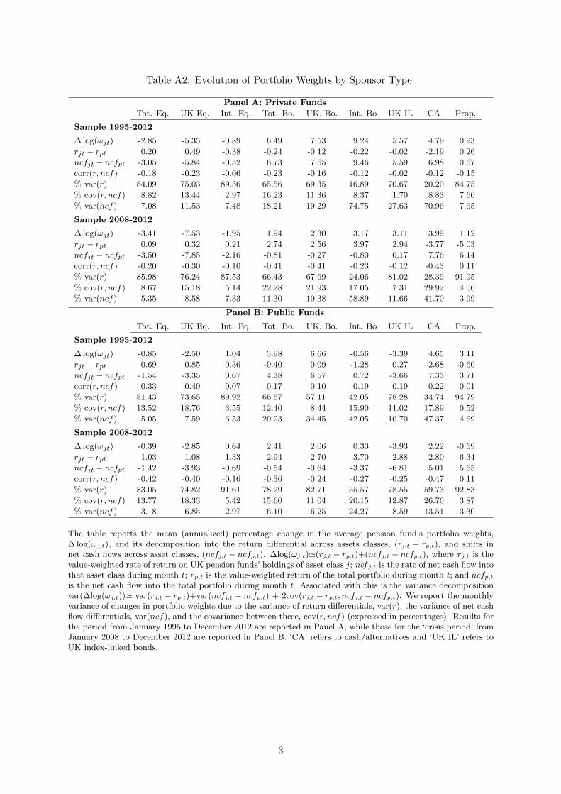
21In the Internet Appendix, Table A2 shows the decomposition of changes in asset weights separately forprivate- and public-sector funds. Of particular interest is the dramatic decrease in equity weighting by private-sector funds during the crisis that is largely driven by strong negative net investment (outflow) effects. Moreover,though private-sector funds’ allocation to international bonds is fairly constant, this masks substantial positivevaluation changes that are offset by negative flow effects.
21
time t − s; and Liq t−s is the time t − s measure of liquidity, as described in Section 5.2.22,23
Panel A of Table 6 reports the aggregate market (Σβ=3∑s=0
βs) and liquidity (Σγ=3∑s=0
γsLiq t−s)
effects, in addition to the individual βs and γs coefficients. There is overwhelming evidence that
pension funds rebalance their portfolios in response to valuation changes, i.e., they behave like
contrarian investors in that they increase (decrease) the return-adjusted weight in asset class j
in response to negative (positive) valuation changes, which are proxied by negative (positive)
returns in the external index associated with asset class j. This is true for equities and especially
for bonds, although not for property, again for liquidity reasons. Pension funds also increase
their allocation to most asset classes (with the exception of international bonds), but especially
to international equities during periods of increased liquidity.
The constant terms in these regressions have an important interpretation. Recall that the
dependent variable captures the component of the change in weight that is due to flow effects.
As a result, the constant measures the time trend in a dynamic model of return-adjusted
weights. It therefore provides useful information about the long-term SAA of pension funds.
The negative constant on UK equities and the positive constant on bonds, for example, reflect
de-risking (i.e., increased maturity matching) that is mainly driven by private-sector funds over
the period. The positive constant on international equities reflects the switch from domestic to
international equities following the ending of tax relief on UK equity dividends in 1997. The
positive constant on index-linked bonds reflects the increasing focus on LDI. Overall, this simple
model is particularly useful for identifying the key determinants of pension funds’ allocation in
equities, with R2s of roughly 20 percent.
Panel B shows that the explanatory power of the model increases during the crisis period
but qualitatively the results are largely unchanged: we again find evidence of a strong rebal-
ancing effect, although this effect is no longer present for UK index-linked bonds. Further,
pension funds significantly decrease their allocation to international equities, UK bonds and
cash/alternatives as liquidity dries up. The results for property are rather different, however,
as pension funds tend to increase their allocation to this asset class not only when the external
property index increases, but also when global liquidity conditions deteriorate.
22Note that we do not have information on peer-group benchmark net investment flows, as the benchmarks onlyprovide direct information on value weights and returns. Thus, we cannot perform the peer-group benchmarkregressions as we did previously for returns. However, we can construct the flow of the average fund based onindividual fund flows, and the average fund’s flow is comparable to a hypothetical peer-group benchmark flow.
23We allow for lags in the right-hand side variables to account for the persistence in the evolution of the flows.This persistence may reflect pension funds’ reluctance to rebalance every month, and their tendency to adjusttheir portfolios only when the actual asset allocation differs significantly from the desired asset allocation.
22
Overall, the results reported in this section suggest that pension funds herd strongly in
subgroups defined by fund size and sponsor type, as one would expect given the institutional
setting of the industry in which they operate. Their herding behavior is not related, however,
to either habit investing or momentum trading, but rather to portfolio rebalancing.
4.2.4 Further Analysis
We subject the previous analysis to two additional exercises. First, we investigate the possibility
that our findings might be driven by the fact that the herding analysis is based on only a small
number of asset classes (compared with earlier studies which instead tend to focus on a large
number of individual securities) and may also be distorted by an adding-up constraint. One
concern, therefore, is whether the herding test employed here displays size distortion (a high
probability of rejecting the null hypothesis of no herding when the null is true, i.e. type I error).
To investigate this issue, we simulate the portfolio for a fixed number of funds (189 equal to
the number of funds in our dataset), but for different number of asset classes, under the null
of no herding. We perform 50,000 iterations; see Section A.II, in the internet Appendix, for a
detailed description of the simulations.
If the Sias’ test works well and displays no size distortion, it should produce a test size of
around 5 percent. Table A4 shows the 95 percent critical values from the empirical distribution,
together with the associated test size, obtained by performing the Sias’ test on the simulated
portfolio flows (Panel A) and on portfolio weights (Panel B). Our analysis suggests that, re-
gardless of the number of asset classes considered, the Sias’ test does not suffer from any size
distortion. Moreover, the fact that these findings hold regardless of whether the test is based
on portfolio flows or weights (also in the case of only 5 asset classes) allows us to conclude that
the Sias’ test works reliably, and does not suffer from any size distortion, even in the presence
of an adding-up constraint.24
Second, we repeat the herding analysis using the original measure proposed by LSV (1992)
(LSV measure, thereafter). The LSV measure tests for cross-sectional temporal dependence
only indirectly, by looking at institutional trades within the same month, while the statistic
of Sias (2004) tests directly for cross-sectional temporal dependence, by looking at investors’
24In the paper, we perform the analysis on return-adjusted weights, which are not subject to any adding-upconstraint. It is possible for return-adjusted weights to increase for all asset classes simultaneously, which is not,of course, possible for portfolios weights. Therefore, as a further check, we also conducted the simulations onportfolio weights directly and still found that the Sias’ test does not suffer from low power, and thus we canexclude that the test is subject to any size distortion, also in the presence of an adding-up constraint.
23
trades over subsequent months. The LSV measure for month t and asset class j is defined as:
H(j, t) = |Raw∆j,t −Raw∆t| −AF (j, t), (11)
where Raw∆j,t is the raw fraction of pension funds buying asset class j in month t, Raw∆t is
the expected proportion of funds buying in that month relative to the number of active funds,
and AF (j, t) is an adjustment factor for asset class j in month t, which accounts for differing
numbers of active funds from month to month. Even if pension funds did not display cross-
sectional temporal dependence, the expected value of |Raw∆j,t−Raw∆t| could be greater than
zero, indicating herding. The adjustment factor AF (j, t) will be large when there are only
a small number of funds that are active in asset class j in month t. Specifically, AF (j, t) is
computed by assuming that the number of funds buying asset class j in month t follows a
binomial distribution with probability Raw∆t (see LSV, 1992, for details).
Table A5, Panel A, presents the LSV measure for each of the seven asset classes and the
total portfolio, with (Tot.) and without (Tot. ex CA) the cash/alternatives class. The LSV
measure is computed for each asset class and month; we then report the time-series averages,
together with the associated t-statistics. We again find that, also according to the LSV measure,
pension funds herd in asset classes. Panel B shows similar results for the analysis performed on
return-adjusted weights. However, unlike the Sias’ test, the LSV measure does not allow us to
determine whether this result is due to pension funds following their own trades or other funds’
trades, or whether pension funds herd in subgroups, which is fundamental to our analysis. For
this reason, we prefer to use the Sias’ test for our core analysis.
4.3 Price Impact
Thus far, we have documented that pension funds both herd and mechanically rebalance their
portfolios in the short term. A related issue is whether this trading behavior generates a price
impact. The typically large size of pension fund trades, coupled with pension fund herding
behavior and their inelastic demand for assets, would suggest that they are in a position to
influence asset-price dynamics, particularly in the market where they are big operators. We
start by asking whether there is a price impact resulting from the trading activity of pension
funds and, if this is the case, whether such a price impact is persistent.
We address both questions by examining the relationship between pension fund demand
24
shocks and both contemporaneous and subsequent returns, given a set of controls. We use
a similar methodology to Dennis and Strickland (2002), among others. We differ, however,
in that we look at the price impact on index returns rather than at the level of individual
securities. This will affect the set of controls we employ, but the spirit of the test remains the
same. Furthermore, we restrict the analysis to UK asset classes, as we expect any price pressures
exerted by UK pension funds to have a stronger impact on domestic than international markets.
Specifically, we organize our analysis around the following regression:
rj,t+h = γj,0 + γj,1CFj,t + γj,2Zj,t + εj,t (12)
where rj,t+h is the return in month t+h of asset class j for h =0,...,12; CFj,t is the net investment
of UK pension funds into asset class j in month t, which is divided by the standard deviation that
is computed over a five-year rolling window; and, Zj,t is the set of control variables, which vary
with the market considered. The set of control variables for UK equities include lagged equity
returns (to capture momentum effects), dividend yields, term spreads, and realized equity return
volatility. The set of control variables for UK bonds include lagged bond returns, term spreads,
the short rate, the five-year break-even inflation rate, and realized bond return volatility.
The results, displayed in Figure 4, show that pension funds trade in the opposite direction
to market movements, therefore providing short-term liquidity to the markets. Specifically,
consistent with Lipson and Puckett (2006), we find that pension funds are net sellers (net
buyers) in months when markets experience price increases (decreases). In fact, for h = 0, the
γj,1 coefficient is negative, and statistically significant, across asset classes. However, the price
impact is not persistent, since for h 6= 0, the γj,1 coefficients are no longer statistically different
from zero. The absence of an effect that is persistent, in turn, suggests that pension fund trades
are uninformed, in the sense of not reflecting changes in expected returns, a finding that is
largely consistent with our earlier results showing that pension funds rebalance their portfolios
in a mechanical fashion. Put simply, the short-term trades of pension funds reflect a passive
strategy – set, for example, by asset-class weight limit restrictions specified in the investment
mandate – rather than an active one that responds to changes in expected returns.
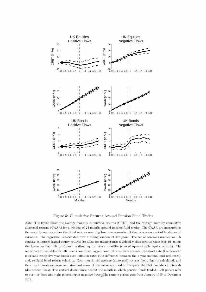
We complement the above analysis on price impact by examining cumulative returns around
pension fund trades, similar to Dennis and Strickland (2002) and Coval and Stafford (2007).
Figure 5 (CRET panels) shows a number of interesting results. First, pension funds tend to
25
sell in response to positive cumulative returns over the preceding 12-months. They also tend to
buy in response to falling returns over the preceding months; however, this effect is somewhat
weaker. Thus, these findings provide further evidence on the rebalancing activity of pension
funds, which complements our earlier results. Second, regardless of whether pension funds
buy or sell, the trend observed in the pre-trade months continues, and eventually intensifies,
during the actual trading month. This graphical representation is largely consistent with the
earlier regression evidence showing that pension funds trade in the opposite direction to market
movements. Third, the trend in cumulative abnormal returns attenuates or actually reverses in
the months following the pension fund trades.
However, the effect of pension fund trades on financial markets will be genuinely stabilizing
only if they move prices towards fundamentals (LSV, 1992; Coval and Stafford, 2007). We shed
light on this issue by looking at the pattern of cumulative absolute abnormal returns (CAAR)
in the months before and after pension fund trades. Abnormal returns are measured as the
observed monthly returns minus the fitted returns resulting from regressing the returns on the
same set of fundamental variables, Zj,t, included in equation (12). Specifically, our hypothesis
is that, if pension fund trades are stabilizing, then the deviation of market returns from their
fundamental values in the months following their trades should be smaller than the deviation
observed in the months preceding their trades. The results are clear-cut (see the CAAR panels
in Figure 5): pension fund trades do not exert a stabilizing effect on prices. In fact, regardless
of the asset class considered, their trades do not alter the slope of the CAAR curve, thereby
indicating that the deviation of returns from their fundamental values is unaffected by pension
funds’ trading activity.
5 Pension Fund Performance
5.1 Investment Performance, Fund Characteristics and Herding Behavior
The analysis so far has largely concentrated on pension funds asset allocations. In this section,
to complete the analysis, we turn to assess the funds’ performance, in an attempt to link the
performance of the funds to their characteristics, such as sector type, fund size, and fund asset
allocation. We also examine to what extent funds’ performance relates to the herding behavior
of the funds.
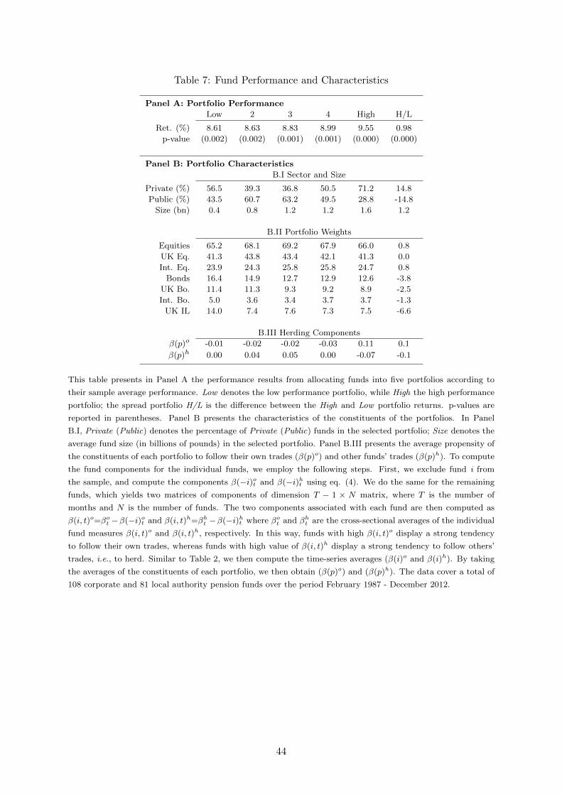
To start with, we allocate funds to five portfolios according to their sample average perfor-
26
mance. Table 7, Panel A, presents the annualized return associated with the five portfolios and
the spread portfolio: Low denotes the lowest performing portfolio, High the highest performing
portfolio, while the spread portfolio H/L is the difference between the High and Low portfolio
returns. The Low and High portfolios generate average returns of 8.60% and 9.55% per annum,
respectively. This implies that the High portfolio outperforms the Low portfolio by roughly 1%
per annum, which, while strongly statistically significant, is economically quite small.
Next, we examine the characteristics of the constituents of the portfolios. Panel B.I shows
that the best performing funds are private: they account for 71% of the funds in the High
portfolio, and only 57% of the funds in the Low portfolio. The panel also shows an almost
monotonic relationship between fund size and fund performance, with the best performing
funds being four times larger than the worst performing funds.25 We also find that the worst
performing funds have a higher weighting in fixed-income and inflation-linked securities than
the best performing funds (Panel B.II). Taken together, these findings show that the worst
performing funds tend to be more mature than the best performing funds.
In Panel B.III, we present the average propensity of the constituents of each portfolio to
follow their own trades (β(p)o) and other funds’ trades (β(p)h). To compute the fund compo-
nents for the individual funds, we employ the following steps. First, we exclude fund i from the
sample, and compute the components β(−i)ot and β(−i)ht using eq. (4). We do the same for
the remaining funds, which yields two matrices of components of dimension T − 1×N matrix,
where T is the number of months and N is the number of funds. The two components associ-
ated with each fund are then computed as β(i, t)o=βot −β(−i)ot and β(i, t)h=βht −β(−i)ht where
βot and βht are the cross-sectional averages of the individual fund measures β(i, t)o and β(i, t)h,
respectively. In this way, funds with high β(i, t)o display a strong tendency to follow their own
trades, whereas funds with high value of β(i, t)h display a strong tendency to follow others’
trades, i.e., to herd. Similar to Table 2, we then compute the time-series averages (β(i)o and
β(i)h). By taking the averages of the constituents of each portfolio, we then obtain (β(p)o) and
(β(p)h), displayed in Panel B.III. We find that the most profitable funds not only tend to follow
more their own trades, but also they tend to herd less. This piece of evidence therefore suggests
that herding might be a drag on the fund performance. However, this effect is economically
small, possibly because all funds tend to display a strong tendency to herd.
25Note that Chen, Hong, Huang and Kubik (2004) instead document that larger funds face significant disec-onomies of scale that limit their ability to move into and out of the more illiquid traded securities in size.
27
The above analysis did not condition on herding propensity, we therefore conduct the fol-
lowing portfolio-sort exercise. We sort the active funds every month into five portfolios by their
tendency to herd, β(i)ht =βht − β(−i)ht . Thus, the constituents of the Low (High) portfolio are
the funds which display little (high) herding propensity. We repeat the analysis for the returns
on the funds’ total portfolios, as well as separately for the returns on the main asset classes
(using the same sorting variable β(i)ht ).
Panel A, Table 8, presents the average annualized returns associated with each of the port-
folios and for the selected asset classes for the 1995-2012 period.26 Although the funds that
herd more tend to generate lower returns than the funds which herd less, these effects are eco-
nomically small (30 basis points for the total portfolio) and statistically insignificant. Also the
returns on the spread portfolios of the individual asset classes are not economically significant,
and are statistically significant only for two asset classes (international equities and total bonds).
Panel B shows that the findings are similar for the ‘crisis period’ 2008-2012.27 Nevertheless,
high-herding funds underperform low-herding funds by 85 basis points during this period, which
is mainly driven by their allocations to international bonds.
In sum, there are small cross-sectional differences in the performance of pension funds,
consistent with evidence that they have a strong tendency to herd. By engaging in herding
activity, funds converge towards the performance of the peer-group fund. However, we also find
that more mature and smaller funds generate lower returns than less mature and larger funds,
respectively, which aligns closely with the evidence documented in Section 4.2.2 that pension
funds herd in subgroups, defined by fund size and sponsor type.
5.2 Factors Driving Pension Fund Returns
Thus far, we have established that pension funds herd around the average fund, which generates
the peer-group average return. A natural question then is: to what extent do the returns of the
peer-group respond to changes in the returns of external benchmarks? More generally, what
drives the returns of pension funds? To answer this question, we assess the responsiveness of
pension fund peer-group benchmark returns (i.e., the returns of the average pension fund) to
changes in external index returns and in liquidity conditions.
We examine peer-group returns by regressing the peer-group benchmark monthly return
26We find similar results for the 1987-2012 sample.27The period of the global financial crisis and its aftermath.
28
(rPGt,j ) of asset j on the relevant market (i.e., external benchmark) return for asset class j
(Mkt j,t), as defined in Section 3.2, and our measure of liquidity (Liq t):
Following Hu, Pan, and Wang (2013), given the high serial correlation in pension fund returns,
we introduce lagged market and liquidity factors. As a result, estimates of the average (peer-
group) pension fund’s total exposure to the market and liquidity factors is given by, respectively,
β1 +β2 (denoted Σβ) and γ1 +γ2 (denoted Σγ). Panel A of Table 9 presents the estimates and
shows that the explanatory power of this simple model is very high, except for cash/alternatives.
We find that the exposure to market risk (Σβ) is close to unity for UK and international equities
as well as for property. This will only be the case if the average pension fund holds the same
securities with the same weights as the market index for each asset class. The coefficient on the
market exposure for the three classes of bonds differs from unity. In the case of international
bonds, the coefficient is 0.68, hence well below unity; the reason for this is that the average
fund’s weightings in its international bond portfolio differs significantly from the external index
weightings.28
Turning to the liquidity factor, the average fund’s allocation to international equities is
significantly and positively exposed to changes in liquidity: increases in liquidity are associated
with higher returns. The same holds for the two conventional bond portfolios, with the liquidity
exposure of international bonds being roughly four times higher than that of domestic bonds.
In contrast, the liquidity exposures are negative for UK index-linked bonds and for property
returns. The regressions for the ‘crisis period’ 2008-12 are reported in Panel B. The results are
broadly similar for market risk exposures although, not surprisingly, the liquidity exposures are
generally larger in absolute size. In particular, the negative exposure of UK index-linked bond
and property returns to the liquidity factor increased significantly during the crisis period.29
28There is a simple explanation for this. Market-weighted international bond indices will be dominated bythe bonds of the most indebted and least credit worthy nations. No institutional investor will hold the marketweighting in international bonds.
29Our measure of liquidity may not adequately reflect the underlying liquidity of the property market. Theliterature on measuring liquidity in the property market is rather scarce. One notable exception is Fisher, Geltnerand Pollakowski (2007) who use a measure of demand pressure to capture property illiquidity. However, thismeasure is not available at monthly frequency. More importantly, when we include this measure in the principalcomponent analysis at a quarterly frequency, we find that its loading on the first principal component has theopposite sign of the other variables. For all these reasons, we decided not to include any measure of illiquidityrelated to the property market.
29
6 Conclusions
Institutional investors are particularly large investors, tend to move in and out of asset classes
at the same time and their net asset demands are often driven by factors other than risk-return
considerations. Of particular interest are pension funds that globally are as large as mutual
funds, but much less is known about their investment behavior. This is mainly due to the
scarcity of available data to analyze. In this paper, we have access to a unique dataset on the
UK pension funds’ monthly allocations to major asset classes over the period 1987-2012. This
dataset allows us to investigate the behavior of private- and public-sector funds over the past
25 years.
We find strong evidence that pension funds do indeed behave like lemmings as they herd
strongly both in asset classes and in clearly defined subgroups. As a consequence, there are
only small cross-sectional differences in the performance of pension funds. The fact that the
subgroups are defined by fund size and sponsor type suggests that this herding behavior directly
stems from the institutional structure of the pension fund industry, as well as the incentives
pension funds have to watch closely their peer group. Specifically, we find that pension funds
herd around the average fund (in their peer-group) in the very short term, and the average
pension fund turns out to be a closet index matcher. We also find that pension funds rebalance
their portfolios in a way that is consistent with meeting their mandate restrictions on asset
weights in the short term, and with maintaining a long-term strategic asset allocation that
matches the maturity of their liabilities. These two features – herding and mechanical portfolio
rebalancing – are the key elements that characterize the asset allocation decisions of pension
funds.
Our results also show that the trading activities of pension funds are consistent with the
notion that they provide short-term liquidity to financial markets as they tend to trade in the
opposite direction to market movements. However, this trading does not have an impact on asset
prices that is persistent. Hence, we do not find evidence that pension funds have a stabilizing
effect on financial markets, in the sense of moving asset prices closer to their fundamental values.
Overall, our findings have important implications for plan sponsors and policy makers re-
sponsible for financial stability: both of which would benefit from the design of an incentive
structure that can better motivate pension funds to move away from ‘short-termism’ and focus
on long-term returns and fundamental value. Indeed the investment decisions of pension funds
30
are at the center of the active policy debate on the risks that the behavior of non-bank financial
institutions pose for financial stability (Feroli, Kashyap, Schoenholtz and Shin, 2014; Haldane,
2014; Domanski, Shin and Sushko, 2015), and this paper adds to that debate by offering a
deeper understanding of pension funds’ traditional investment behavior.
31
A Appendix: A Closer Look at Herding in Subgroups
In this section, we describe the herding tests implemented in Section 4.2.2, where we group funds
according to the sponsor type (private-sector and public-sector) and by size (small, medium and
large).
Following Others by Size. We group funds into terciles according to their total assets.
We do this for each month t, so that funds may migrate from one group to another as funds
enter, or exit, the sample. We therefore end up with three groups of funds: small, medium
and large. We measure small funds’ average contribution from following small funds and the
average contribution from following other medium and large funds. The average same-sector-
type herding contribution for small funds at time t is given by the second term in eq. (4) limited
to small funds averaged over the J asset classes:
Avg same-sizeSmallt =
1
J
J∑j=1
[Sj,t∑n=1
S∗j,t−1∑m=1,m 6=n
(Dn,j,t −RawW∆t
Sj,t
Dm,j,t−1 −RawW∆t−1
S∗j,t−1
)],
(A.1)
where Sj,t is the number of small funds trading asset class j in month t; S∗j,t−1 is the number
of other small funds trading asset class j in month t; Dn,j,t is a dummy variable that equals
unity (zero) if pension fund n buys (sells) asset class j at time t; Dm,t is a dummy variable
that equals unity (zero) if pension fund m buys (sells) asset class j at time t. The average
different-sector-type herding contribution for small funds at time t is given by the second term
in eq. (4) limited to small funds following medium and large funds averaged over the J asset
classes:
Avg different-sizeSmallt =
1
J
J∑j=1
[Sj,t∑n=1
MLj,t−1∑m=1,m 6=n
(Dn,j,t −RawW∆t
Sj,t
Dm,j,t−1 −RawW∆t−1
MLj,t−1
)],
(A.2)
where MLj,t−1 is the number of medium and large funds trading asset class j in month t − 1.
All t-statistics are computed from time-series standard errors. The average same-size herding
contribution for medium (large) funds is computed in a similar fashion to eq. (A.1), and the
average different-size herding contribution for medium and large funds similar to eq. (A.2).
Following Others by Size and Type. We perform a 3×2 double sort in which we classify
funds into terciles according to their size (small, medium, large) and sponsor type (private,
public). The average same-size&type herding contribution for small private-sector funds at
time t is given by the second term in eq. (4) limited to small private-sector funds averaged over
the J asset classes:
Avg same-size&typeSmall Privatet =
32
=1
J
J∑j=1
[SCj,t∑n=1
SC∗j,t−1∑m=1,m 6=n
(Dn,j,t −RawW∆t
SCj,t
Dm,j,t−1 −RawW∆t−1
SC∗j,t−1
)], (A.3)
where SCj,t is the number of small private-sector funds trading asset class j in month t; SC∗j,t−1
is the number of other small private-sector funds trading asset class j in month t; Dn,j,t is a
dummy variable that equals unity (zero) if pension fund n buys (sells) asset class j at time t;
Dm,t is a dummy variable that equals unity (zero) if pension fund m buys (sells) asset class j
at time t. The average different-size&type herding contribution for small private-sector funds
at time t is given by:
Avg different-size&typeSmall Privatet =
=1
J
J∑j=1
[SCj,t∑n=1
Oj,t−1∑m=1,m6=n
(Dn,j,t −RawW∆t
SCj,t
Dm,j,t−1 −RawW∆t−1
Oj,t−1
)], (A.4)
where Oj,t−1 is the number of funds other than small private-sector funds (small public, medium
public and private, and large public and private) trading asset class j in month t− 1.
We then restrict the group of other-different by focusing on other funds of different type but
the same size. The average different-type herding contribution for small private-sector funds
at time t is given by:
Avg different-typeSmall Privatet =
=1
J
J∑j=1
[SCj,t∑n=1
SLAj,t−1∑m=1,m6=n
(Dn,j,t −RawW∆t
SCj,t
Dm,j,t−1 −RawW∆t−1
SLAj,t−1
)], (A.5)
where SLAj,t−1 is the number of other small public-sector funds trading asset class j in month
t − 1. Average contributions for small public, medium public and private, large public and
private funds are computed using a similar method.
B Appendix: Measuring Liquidity
Our measure of liquidity consists of the first principal component of the negative of the change
in the US TED spread, the negative of the change in the UK TED spread, the Pastor and
Stambaugh (2003) measure of liquidity, the negative of the change in the VIX volatility index,
and the negative of the change in the noise measure of Hu, Pan, and Wang (2013). We describe
each measure in turn.
TED spread. The US TED spread is defined as the interest rate difference between 3-month
33
eurodollar LIBOR and 3-month US Treasury bills. The UK TED spread is defined similarly
using sterling equivalents. A large spread should be related to lower liquidity, reflecting among
other things the willingness of banks to provide funding in the interbank market (Brunnermeier,
2009). We use the TED spread both for the US and the UK.
Pastor and Stambaugh liquidity measure. The Pastor and Stambaugh liquidity measure is
constructed for the US stock market based on price reversals. Specifically, this measure focuses
on an aspect of liquidity associated with temporary price fluctuations induced by order flows.
The basic idea is that less liquid stocks are expected to experience more severe reversals in
return for a given dollar value. We refer the reader to Pastor and Stambaugh (2003) for more
details on the construction of the liquidity measure. However, it is worth noting here that in
contrast to the other measures used, this is a measure of liquidity rather than illiquidity.
Chicago Board Options Exchange Market Volatility Index (VIX). VIX represents one mea-
sure of the market’s expectation of stock market volatility over the next 30 day period. VIX
is often referred to as the fear index. During episodes of risk panics, liquidity usually drops
(Bacchetta, Tille and van Wincoop, 2012). Therefore, although VIX is not a ‘pure’ measure of
illiquidity, it increases in periods of low liquidity, and may complement the information provided
by the other measures used.
Hu, Pan and Wang (2013) noise measure. The noise measure is a market wide illiquidity
measure that exploits the connection between the arbitrage capital in the market and observed
price deviations in US Treasury bonds. It captures the noise in the yield curve, which can result,
for example, from low value trades by hedge funds. Using the CRSP Daily Treasury database,
the authors construct the noise measure by first backing out, day by day, a smooth zero-coupon
yield curve, and then use this yield curve to price all available bonds on that day. Associated
with each bond is the deviation of its market yield from the model yield. Aggregating the
deviations across all bonds by calculating the root mean squared error, they obtain their noise
measure. A large value of the noise measure should be related to lower liquidity. We refer the
reader to Hu, Pan and Wang (2013) for more details on the construction of the noise measure.
34
References
Andonov, A., R. Bauer, and M. Cremers, 2013, Pension Fund Asset Allocation and Li-ability Discount Rates: Camouflage and Reckless Risk Taking by U.S. Public Plans? mimeo,Maastricht University.
Bacchetta, P., C. Tille, and E. van Wincoop, 2012, Self-Fulfilling Risk Panics, AmericanEconomic Review 102, 3674–3700.
Banerjee, A., 1992, A Simple Model of Herd Behavior, American Economic Review 88, 724-48.
Bank of England, 2014, Procyclicality and Structural Trends in Investment Allocation byInsurance Companies and Pension Funds, A Discussion Paper by the Bank of England and theProcyclicality Working Group.
Benzoni, L., P. Collin-Dufresne, and R. S. Goldstein, 2007, Portfolio Choice over theLife-Cycle when the Stock and Labor Markets are Cointegrated, Journal of Finance 62, 2123-67.
Blake, D., 2003, Pension Schemes and Pension Funds in the United Kingdom, Oxford Univer-sity Press, Oxford.
Blake, D., B. N. Lehmann, and A. Timmermann, 1999, Asset Allocation Dynamics andPension Fund Performance, Journal of Business 72, 429-61.
Blake, D., G. A. Rossi, A. Timmermann, I. Tonks, and R. Wermers, 2013, DecentralizedInvestment Management: Evidence from the Pension Fund Industry, Journal of Finance 68,1133-77.
Blake, D., and A. Timmermann, 2002, Performance Benchmarks for Institutional Investors:Measuring, Monitoring and Modifying Investment Behaviour, in John Knight and StephenSatchell (eds) Performance Measurement in Finance: Firms, Funds and Managers, ButterworthHeinemann, Oxford, 108-141.
Bikhchandani, S., D. Hirshleifer, and I. Welch, 1992, A Theory of Fads, Fashion, Cus-tom, and Cultural Change as Informational Cascades, Journal of Political Economy 100, 992-1026.
Brunnermeier, M. K., 2009, Deciphering the Liquidity and Credit Crunch 2007–2008, Journalof Economic Perspectives 23, 77–100.
Brunnermeier, M., and L. H. Pedersen, 2009, Market Liquidity and Funding Liquidity,Review of Financial Studies 22, 2201-38.
Chan, L. K. C., and J. Lakonishok, 1995, The Behavior of Stock Prices Around InstitutionalTrades, Journal of Finance 50, 1147-1174.
Chen, J., H. Hong, M. Huang, and J. D. Kubik, 2004, Does Fund Size Erode MutualFund Performance? The Role of Liquidity and Organization, American Economic Review 94,1276-1302.
Choi, N., and R. Sias, 2009, Institutional Industry Herding. Journal of Financial Economics94(3), 469-491.
Coval, J., and E. Stafford, 2007, Asset Fire Sales (and Purchases) in Equity Markets,Journal of Financial Economics 86, 479-512.
Cremers, M., Ferreira, M. A., Matos, P. P., and L. T. Starks, 2015. Indexing and Ac-tive Fund Management: International Evidence. Journal of Financial Economics, forthcoming.
35
Dennis, P.J., and D. Strickland, 2002, Who Blinks in Volatile Markets, Individuals orInstitutions?, Journal of Finance 57, 1923-1949.
Domanski, D., Shin, H.S., and V. Sushko, 2015, The Hunt for Duration: Not Waiting ButDrowning?, BIS Working Papers 519.
Feroli, M., A. Kashyap, K. Schoenholtz, and H. S. Shin, 2014, Market Tantrums andMonetary Policy, Report for the 2014 US Monetary Policy Forum.
Financial Times, 2014, Deciding to Fire the Fund Manager - A Rough Guide. Financial Times,9 November 2014.
Fisher, J. D., D. Geltner, and H. Pollakowski, 2007, A Quarterly Transactions-BasedIndex of Institutional Real Estate Investment Performance and Movements in Supply and De-mand. Journal of Real Estate Finance and Economics 34(1), 5-33.
Froot, K. A., D. S. Scharfstein, and J. C. Stein, 1992, Herd on the Street: InformationalInefficiencies in a Market with Short-term Speculation, Journal of Finance 47, 1461-84.
Greenwood, R., and D. Vayanos, 2010, Price Pressure in the Government Bond Market,American Economic Review Papers & Proceedings100(2), 585-90.
Grinblatt, M., and S. Titman, 1989, Portfolio Performance Evaluation: Old Issues and NewInsights, Review of Financial Studies 2, 393-422.
Grinblatt, M., and S. Titman, 1993, Performance Measurement without Benchmarks: AnExamination of Mutual Fund Returns, Journal of Business 66, 47-68.
Grinblatt, M., S. Titman, and R. Wermers, 1995, Momentum Investment Strategies,Portfolio Performance, and Herding: A Study of Mutual Fund Behavior, American EconomicReview 85, 1088-1105.
Haldane, G. A., 2014, The Age of Asset Management? Speech given at the London BusinessSchool (4 April).
Hu, X., J. Pan, and J. Wang, 2013, Noise as Information for Illiquidity, Journal of Finance68, 2223-72.
Huberman, G., and P. Sengmueller, 2004, Performance and Employer Stock in 401(k)Plans, Review of Finance 8, 403-443.
Kyle, A. S., 1985, Continuous Auctions and Insider Trading, Econometrica 53(6), 1315-35.
Lakonishok, J., A. Shleifer, and R. W. Vishny, 1992, The Impact of Institutional Tradingon Stock Prices, Journal of Financial Economics 32, 23-43.
Lipson, M., and A. Puckett, 2006, Volatile Markets and Institutional Trading, University ofMissouri, mimeo.
Lucas, D. J., and S. Zeldes, 2009, How Should Public Pension Funds Invest?, AmericanEconomic Review P&P 99, 527-532.
Malkhozov, A., Mueller, P., Vedolin, A. and G. Venter, 2015, Mortgage Risk and theYield Cruve. Review of Financial Studies, forthcoming.
Nofsinger, J., and R. Sias, 1999, Herding and Feedback Trading by Institutional and Indi-vidual Investors, Journal of Finance 54, 2263-2295.
36
Pastor, L., and R. F. Stambaugh, 2003, Liquidity Risk and Expected Stock Returns, Journalof Political Economy 111, 642-85.
Pennacchi, G., and M. Rastad, 2011, Portfolio Allocation for Public Pension Funds, Journalof Pension Economics and Finance, 10, 221-45.
Reca, B., Sias, R., and H. J. Turtle, 2014, Hedge Fund Crowds and Mispricing, ManagementScience, forthcoming.
Scharfstein, D. S., and J. C. Stein, 1990, Herd Behavior and Investment, American Eco-nomic Review 80, 465-479.
Shleifer, A., 1985, A Theory of Yardstick Competition, Rand Journal of Economics, 16, 319-27.
Sialm, C., Starks, L. T., and H. Zhang, 2015, Defined Contribution Pension Plans: Stickyor Discerning Money?, Journal of Finance 70, 805-828.
Sialm, C., Starks, L. T., and H. Zhang, 2015, Defined Contribution Pension Plans: MutualFund Asset Allocation Changes, American Economic Review 105, 432-436.
Sias, R., 2004, Institutional Herding, Review of Financial Studies 17(1), 165-206.
Sias, R.W., Starks, L., and S. Titman, 2006, Changes in Institutional Ownership and StockReturns: Assessment and Methodology, Journal of Business 79, 2869-2910.
Stein, J.C., 2009, Sophisticated Investors and Market Efficiency, Journal of Finance, 64, 1517-48.
Timmermann, A., and D. Blake, 2005, International Asset Allocation with Time-VaryingInvestment Opportunities, Journal of Business 78, 71-98.
Tonks, I., 2005, Performance Persistence of Pension Fund Managers, Journal of Business 78,1917-42.
Wermers, R., 1999, Mutual Fund Trading and the Impact on Stock Prices, Journal of Finance54, 581-622.
Wermers, R., 2000, Mutual Fund Performance: An Empirical Decomposition into Stock-Picking Talent, Style, Transaction Costs, and Expenses, Journal of Finance 55, 1655-95.
WM Company, 1997, Strategic Benchmarks – The Universe is Dead; Long Live the Universe!,WM Research and Consultancy, 1-16.
37
Table 1: Summary Statistics: UK Pension Fund Returns
Panel A: All Pension Funds
Mean Med. St.D. Skew. Kurt. ρ1 ρ2 nobs
Total Assets 8.9 12.0 11.4 -1.13 7.55 0.11 -0.10 48030
Total Equities 9.4 13.6 15.5 -1.05 6.45 0.10 -0.12 47229
UK Equities 10.0 15.2 15.8 -0.95 6.81 0.09 -0.12 46847
Total Bonds 8.4 9.8 5.2 0.06 3.48 0.17 -0.02 22354
UK Bonds 8.8 9.1 5.8 0.04 3.33 0.14 -0.05 21795
Int. Bonds 7.6 5.2 6.4 1.23 8.65 0.15 0.05 18092
UK IL 8.2 7.9 7.1 0.54 5.70 0.01 -0.17 17651
Cash/Alt. 5.7 5.1 1.1 0.35 3.78 0.83 0.80 23170
Property 7.2 8.2 3.7 -1.89 10.49 0.82 0.75 19787
The table reports summary statistics on UK pension fund returns. For each month t, we take the cross-sectionalmean of the available pension funds’ annualized returns. We then report: the time series mean (Mean); median(Med.); standard deviation (St.D.); skewness (Skew.); kurtosis (Kurt.); the first- (ρ1) and second-order (ρ2)autocorrelation coefficients; and the number of observations (nobs). We present summary statistics for thefollowing asset classes: total assets, total equities, UK equities, international equities, total bonds, UK bonds,international bonds, UK index-linked (UK IL) bonds, cash/alternatives and property. Panel A refers to thefull sample of pension funds, whereas Panel B focuses on private-sector funds (i.e., corporates) and Panel C onpublic-sector funds (i.e., local authorities). The data cover a total of 108 corporate and 81 local authority pensionfunds over the period January 1987 - December 2012.
The table reports in Panel A the sample average βt resulting from estimating the regressions ∆j,t = βt∆j,t−1+εj,t,where ∆j,t is the standardized raw fraction of institutions buying asset class j as defined in eq. (2) in Section 4.The t-statistics (reported in parentheses) are computed from time-series standard errors. The time t correlationβt is then decomposed as βt = ρ (∆j,t,∆j,t−1) = βo
t +βht , as in eq. (4), where βo
t indicates pension funds ‘followingtheir own trades’ into and out of the same asset class, and βh
t indicates pension funds ‘following others’ (herding).
We report the sample average βot and βh
t with the associated time-series t-statistics in parentheses. Specification(1) includes the seven asset classes: UK equities, international equities, UK bonds, international bonds, UKindex-linked bonds, cash/alternatives and property. Specification (2) excludes cash/alternatives, focusing on theremaining six asset classes. In Panel B, we repeat the analysis by replacing the demand measure based on cashflows with the demand measure based on return adjusted-weights (∆j,t); we identify pension fund n as a buyer(seller) of asset class j, if the return-adjusted portfolio weight of asset class j increased (decreased), i.e., the flowdifferential ncf n,j,t − ncf n,p,t is positive (negative). The data cover the period January 1987 - December 2012.
39
Table 3: Herding in Subgroups Defined by Fund Size and Sponsor Type: Single Sort
The table reports the decomposition of a measure of herding whereby pension funds ‘following others’ is de-composed into pension funds following others of the Same type and Other type. The analysis is based on thestandardized fraction of pension funds increasing/decreasing the return-adjusted weight in asset j in month t
(∆j,t). Same refers to the average contribution to the correlation from each pension fund following other pensionfunds with the same characteristics, see eq. (7). Other refers to the average contribution to the correlation fromeach pension fund following other pension funds with different characteristics, see eq. (8). Numbers are reportedin percent. Panel A focuses on the sponsor type, private-sector funds (i.e., those sponsored by corporates) vs.public-sector funds (i.e., those sponsored by local authorities). Panel B focuses on the size differences, wherebyfunds are sorted into small, medium and large in each period t. (1) All Assets includes the seven asset classes:UK equities, international equities, UK bonds, international bonds, UK index-linked bonds, cash/alternativesand property. (2) All Assets ex CA excludes cash/alternatives, focusing on the remaining six asset classes. Allt-statistics (reported in parentheses) are computed from time-series standard errors.
40
Table 4: Herding in Subgroups Defined by Fund Size and Sponsor Type: Double Sort
The table reports the decomposition of a measure of herding whereby pension funds ‘following others’ is decom-posed into pension funds following others of the Same type and Other type, controlling for size. The analysis isbased on the standardized fraction of pension funds increasing/decreasing the return-adjusted weight in asset j in
month t (∆j,t). Funds are sorted according to their size and then for each tercile into private- and public-sector.Same refers to the average contribution to the correlation from each pension fund following other pension fundsof the same size and sponsor type, see eq. (A.3). Other refers to the average contribution to the correlationfrom each pension fund following other pension funds of the same size but different sponsor type, see eq. (A.5).Numbers are reported in percent. Panel A includes the seven asset classes: UK equities, international equi-ties, UK bonds, international bonds, UK index-linked bonds, cash/alternatives and property. Panel B excludescash/alternatives (ex CA), focusing on the remaining six asset classes. All t-statistics (reported in parentheses)are computed from time-series standard errors.
41
Table 5: Evolution of Portfolio Weights
Panel A: 1995-2012
Tot.Eq. UK Eq. Int.Eq. Tot.Bo. UK Bo. Int.Bo. UK IL CA Prop.
The table reports the mean (annualized) percentage change in the average pension fund’s portfolio weights,∆ log(ωj,t), and its decomposition into the return differential across assets classes, (rj,t − rp,t), and shifts innet cash flows across asset classes, (ncfj,t − ncfp,t). ∆log(ωj,t)'(rj,t − rp,t)+(ncfj,t − ncfp,t), where r j,t is thevalue-weighted rate of return on UK pension funds’ holdings of asset class j ; ncf j,t is the rate of net cash flow intothat asset class during month t ; rp,t is the value-weighted return of the total portfolio during month t ; and ncfp,tis the net cash flow into the total portfolio during month t. Associated with this is the variance decompositionvar(∆log(ωj,t))' var(rj,t − rp,t)+var(ncfj,t − ncfp,t) + 2cov(rj,t − rp,t, ncfj,t − ncfp,t). We report the monthlyvariance of changes in portfolio weights due to the variance of return differentials, var(r), the variance of net cashflow differentials, var(ncf), and the covariance between these, cov(r,ncf) (expressed in percentages). Results forthe period from January 1995 to December 2012 are reported in Panel A, while those for the global financial crisisand its aftermath from January 2008 to December 2012 are reported in Panel B. ‘CA’ refers to cash/alternativesand ‘UK IL’ refers to UK index-linked bonds.
42
Table 6: Regressions of Net Cash Flows on Asset Market Returns and Liquidity
The table reports regressions of changes in aggregate portfolio weights due to the net cash flow rate differential
component ncf j,t -ncf p,t, denoted by NCFj,t, on current and past asset market returns and liquidity effects.
Specifically, we estimate NCFj,t =α +∑3
s=0 βsMktj,t−s+∑3
s=0 γsLiqt−s+εt. Mktj,t is the time-t return on therelevant external benchmark for asset class j. The measure of liquidity Liqt is the first principal component of thenegative of the change in the US TED spread, the negative of the change in the UK TED spread, the Pastor andStambaugh (2003) measure of liquidity, the negative of the change in the VIX volatility index, and the negativeof the change in the noise measure of Hu, Pan, and Wang (2013). Σβ (Σγ) denotes the sum of contemporaneousand lagged betas (gammas). The regression is at a monthly frequency for the period from January 1995 toDecember 2012 in Panel A, and for the global financial crisis and its aftermath from January 2008 to December2012 in Panel B. R2s denote the adjusted R-squared. t-statistics are computed by using Newey-West standarderrors. a, b, and c denote the 1-, 5-, and 10-percent significance levels, respectively. α is the constant term inthe regression, CA refers to cash/alternatives and UK IL refers to UK index-linked bonds.
The table reports regressions of the peer-group benchmark monthly return (rPGj,t ) of asset j on the relevant
(external benchmark) market return for asset class j and liquidity. Specifically, we estimate rPGj,t = α+β1Mktj,t+
β2Mktj,t−1 +γ1Liqt +γ2Liqt−1 +εt. Mktj,t is the time-t return of the relevant external benchmark for asset classj. The measure of liquidity Liqt is the first principal component of the negative of the change in the US TEDspread, the negative of the change in the UK TED spread, the Pastor and Stambaugh (2003) measure of liquidity,the negative of the change in the VIX volatility index, and the negative of the change in the noise measure ofHu, Pan, and Wang (2013). Σβ (Σγ) denotes the sum of contemporaneous and lagged betas (gammas) withthe associated t-statistics beneath. The regression is at a monthly frequency for the period from January 1995to December 2012 in Panel A, and for the ‘crisis period’ from January 2008 to December 2012 in Panel B. R2sdenote the adjusted R-squareds. t-statistics are computed by using the Newey-West standard errors. a, b, and cdenote the 1-, 5-, and 10-percent significance levels, respectively. α is the constant term in the regression, ‘CA’refers to cash/alternatives and ‘UK IL’ refers to UK index-linked bonds.
46
87 91 95 99 03 07 110
100
200
300
400Total Assets
87 91 95 99 03 07 110
20
40
60
80Bonds
87 91 95 99 03 07 110
50
100
150
200Equities
87 91 95 99 03 07 110
5
10
15
20
25
30Cash/Alternatives
87 91 95 99 03 07 110
5
10
15
20
25
30Index−linked
87 91 95 99 03 07 110
5
10
15
20
25Property
Local Authorities
Corporates
Figure 1: UK Pension Fund Asset Holdings by Sponsor Type (in Billion Pounds)
Note: The figure shows UK private- and public-sector funds’ total asset holdings as well as their holdings inequities, bonds, UK inflation-linked bonds, cash/alternatives and property for the period from January 1987 toDecember 2012.
47
87 90 93 95 98 01 04 06 09 120
20
40
60
80
100
Time
Ass
et W
eigh
ts (
in %
)
Corporates
Property
UK Index−linked
Cash/Alt.
Bonds
Equities
87 90 93 95 98 01 04 06 09 120
20
40
60
80
100
Time
Ass
et W
eigh
ts (
in %
)
Local Authorities
Property
UK Index−linked
Cash/Alt.
Bonds
Equities
Figure 2: Asset Weights by Sponsor Type (in %)
Note: The figure shows UK private- and public-sector funds’ asset allocation weightings in equities, bonds, UKinflation-linked bonds, cash/alternatives and property for the period from January 1987 to December 2012.
48
87 91 95 99 03 07 110
20
40
Total Assets
87 91 95 99 03 07 110
10
20
Bonds
87 91 95 99 03 07 110
5
10
15
Equities
87 91 95 99 03 07 110
5
10
15
Cash/Alternatives
87 91 95 99 03 07 110
2
4
UK Index−linked
87 91 95 99 03 07 110
2
4
6
8
Property
Figure 3: Cumulative Net Cash Flows by UK Pension Funds (in Billion Pounds)
Note: The figure shows UK pension funds cumulative net cash flows (net investment) in total assets and inequities, bonds, UK index-linked bonds, cash/alternatives and property for the period from January 1987 toDecember 2012.
49
0 5 10
−1
0
1
Months
UK
Equ
ities
All Funds1995−2012
0 5 10
−1
0
1
Months
All Funds1995−2007
0 5 10
−0.5
0
0.5
Months
UK
Bon
ds
0 5 10
−0.5
0
0.5
Months
Figure 4: Price Impact
Note: The figure shows the price impact of pension fund trades on UK equities and bonds. We use the returnson the external benchmark indices described in Section 3.2. Specifically, we organize our analysis around thefollowing regression:
rj,t+h = γj,0 + γj,1CFj,t + γj,2Zj,t + εj,t
and plot γj,1 for h=0,...,12 (solid line) together with 95% confidence intervals (dot-dashed line), calculated using
Newey-West standard errors. The set of control variables for UK equities include: lagged equity returns (to allow
for momentum); dividend yields; term spreads (the 10- minus the 2-year nominal gilt rates); and, realized equity
return volatility (the sum of squared daily equity returns). The set of control variables for UK bonds include
lagged bond returns; term spreads; the short rate (the 3-month interbank rate); five-year break-even inflation
rate (the difference between the 5-year nominal and real rates); and, realized bond return volatility (the sum of
squared daily bond returns). Left panels show the results for the 1995-2012 sample period, whereas right panels
exclude the 2008-12 crisis period. Source: Datastream, Bank of England and authors’ calculations.
50
t−12 t−9 t−6 t−3 t t+3 t+6 t+9 t+12−10
0
10
20
30
UK Equities Positive Flows
CR
ET
(in
%)
t−12 t−9 t−6 t−3 t t+3 t+6 t+9 t+12−10
0
10
20
30
UK Equities Negative Flows
CR
ET
(in
%)
t−12 t−9 t−6 t−3 t t+3 t+6 t+9 t+120
20
40
60
CA
AR
(in
%)
t−12 t−9 t−6 t−3 t t+3 t+6 t+9 t+120
20
40
60
CA
AR
(in
%)
t−12 t−9 t−6 t−3 t t+3 t+6 t+9 t+12−2
0
2
4
6
UK Bonds Positive Flows
CR
ET
(in
%)
t−12 t−9 t−6 t−3 t t+3 t+6 t+9 t+12−2
0
2
4
6
UK Bonds Negative Flows
CR
ET
(in
%)
t−12 t−9 t−6 t−3 t t+3 t+6 t+9 t+120
10
20
30
40
50
Months
CA
AR
(in
%)
t−12 t−9 t−6 t−3 t t+3 t+6 t+9 t+120
10
20
30
40
50
Months
CA
AR
(in
%)
Figure 5: Cumulative Returns Around Pension Fund Trades
Note: The figure shows the average monthly cumulative returns (CRET) and the average monthly cumulative
abnormal returns (CAAR) for a window of 24-months around pension fund trades. The CAAR are measured as
the monthly returns minus the fitted returns resulting from the regression of the returns on a set of fundamental
variables. The regression is estimated over a rolling window of five years. The set of control variables for UK
equities comprise: lagged equity returns (to allow for momentum); dividend yields; term spreads (the 10- minus
the 2-year nominal gilt rate); and, realized equity return volatility (sum of squared daily equity returns). The
set of control variables for UK bonds comprise: lagged bond returns; term spreads; the short rate (the 3-month
interbank rate); five-year break-even inflation rates (the difference between the 5-year nominal and real rates);
and, realized bond return volatility. Each month, the average (abnormal) returns (solid line) is calculated, and
then the time-series mean and standard error of the mean are used to compute the 95% confidence intervals
(dot-dashed lines). The vertical dotted lines delimit the month in which pension funds traded. Left panels refer
to positive flows and right panels depict negative flows. The sample period goes from January 1995 to December
2012.51
Internet Appendix (not for publication)
The Market for Lemmings: The Herding Behaviour of Pension Funds
by
David Blake, Lucio Sarno and Gabriele Zinna
Table of Content Internet Appendix
• Section A.I: Summary Statistics, Herding and Evolution of Aggregate Portfolio Weights
The table reports summary statistics of pension fund peer-group benchmark returns. We report: the time seriesmean (Mean); median (Med.); standard deviation (St.D.); skewness (Skew.); kurtosis (Kurt.); the first- (ρ1)and second-order (ρ2) autocorrelation coefficients; and the number of observations (nobs). We presentsummary statistics for the following asset classes: total assets, total equities, UK equities, internationalequities, total bonds, UK bonds, international bonds, UK index-linked (UK IL) bonds, cash/alternativesand property. Panel A refers to the full sample of pension funds, whereas Panel B focuses on private-sectorfunds (i.e., those sponsored by corporates) and Panel C on public-sector funds (i.e., those sponsored bylocal authorities).
2
Table A2: Evolution of Portfolio Weights by Sponsor Type
Panel A: Private Funds
Tot. Eq. UK Eq. Int. Eq. Tot. Bo. UK. Bo. Int. Bo UK IL CA Prop.
The table reports the mean (annualized) percentage change in the average pension fund’s portfolio weights,∆ log(ωj,t), and its decomposition into the return differential across assets classes, (rj,t − rp,t), and shifts innet cash flows across asset classes, (ncfj,t − ncfp,t). ∆log(ωj,t)'(rj,t − rp,t)+(ncfj,t − ncfp,t), where r j,t is thevalue-weighted rate of return on UK pension funds’ holdings of asset class j ; ncf j,t is the rate of net cash flow intothat asset class during month t ; rp,t is the value-weighted return of the total portfolio during month t ; and ncfp,tis the net cash flow into the total portfolio during month t. Associated with this is the variance decompositionvar(∆log(ωj,t))' var(rj,t − rp,t)+var(ncfj,t − ncfp,t) + 2cov(rj,t − rp,t, ncfj,t − ncfp,t). We report the monthlyvariance of changes in portfolio weights due to the variance of return differentials, var(r), the variance of net cashflow differentials, var(ncf), and the covariance between these, cov(r, ncf) (expressed in percentages). Results forthe period from January 1995 to December 2012 are reported in Panel A, while those for the ‘crisis period’ fromJanuary 2008 to December 2012 are reported in Panel B. ‘CA’ refers to cash/alternatives and ‘UK IL’ refers toUK index-linked bonds.
3
Table A3: Momentum Trading
Cash Flows Adj. Weights
avg(β1,t) avg(β2,t) avg(β1,t) avg(β2,t)
(1) 42.96 −4.18 54.50 −5.02
[19.77] [-1.73] [26.28] [-2.09]
(2) 44.95 −6.91 50.29 −6.97
[17.92] [-2.55] [18.99] [-2.36]
The table reports the average betas and time-series t-statistics resulting from the following cross-sectional re-gressions
∆j,t = β1,t∆j,t−1 + β2,trPGj,t−1 + εj,t,
where ∆j,t is the standardized fraction of pension funds buying asset class j (Panel: Cash Flows), or increasingthe return-adjusted weight in j in month t (Panel: Adj. Weights) and rPG
j,t−1 is the standardized peer-group returnof asset j in month t. Specification (1) includes the seven asset classes: UK equities, international equities, UKbonds, international bonds, UK index-linked bonds, cash/alternatives and property. Specification (2) excludescash/alternatives, focusing on the remaining six asset classes.
4
87 93 98 04 09−20
−10
0
10UK Equities
All
87 93 98 04 090
5
10
15
20Int. Equities
87 93 98 04 09−15
−10
−5
0
5
Cor
pora
tes
87 93 98 04 090
2
4
6
8
87 93 98 04 09−2
0
2
4
Loca
l Aut
horit
ies
87 93 98 04 090
5
10
15
Figure A1: Cumulative Equity Flows (in Billion Pounds)
Note: The figure shows UK private- and public-sector cumulative flows (net investment) in total, UK andinternational equities for the period from January 1987 to December 2012.
5
87 91 95 99 03 07 11
0
5
10
15
UK Bonds
All
87 91 95 99 03 07 110
2
4
6
Int. Bonds
87 91 95 99 03 07 110
2
4
UK Index−linked
87 91 95 99 03 07 11
0
5
10
Cor
pora
tes
87 91 95 99 03 07 110
1
2
3
4
87 91 95 99 03 07 110
1
2
3
4
87 91 95 99 03 07 11−2
0
2
4
6
Loca
l Aut
horit
ies
87 91 95 99 03 07 110
1
2
3
87 91 95 99 03 07 110
0.5
1
1.5
Figure A2: Cumulative Bond Flows (in Billion Pounds)
Note: The figure shows UK private- and public-sector cumulative flows (net investment) in UK and internationalconventional bonds and in UK index-linked bonds for the period from January 1987 to December 2012.
6
A.II Herding Test on Simulated Portfolio Flows and Weights
Here, we simulate the fund portfolio for a fixed number of funds (nF) and for different numbers
of asset classes (nA), or securities, under the no herding assumption. For a given fund i, and
a fixed number of assets nA, we simulate the fund i’s portfolio. To do that, for each asset
class j, we simulate the fund net investment (CF (1 : T, i, j)) and returns (r(1 : T, i, j)), where
1:T is the time period. Having fixed the initial holdings at t = 0 for the asset class j, we
then recover the z-iteration holdings (stock) by using the following dynamics, Hz(t+ 1, i, j) =
Hz(t, i, j)×(1+r(t+1, i, j))+CF (t+1, i, j), as in Blake, Lehmann and Timmerman (1999). The
weights associated with the z-iteration are then easily computed. We repeat the same procedure
for each fund in turn. Then, for the z-iteration portfolio, we compute the Sias’ (2004) herding
measure:
∆zj,t = βzt∆
zj,t−1 + εzj,t. (A.II.1)
and the associated test statistics. We repeat the same steps for Z iterations. We therefore
recover the empirical distributions for the βz =∑T
t=1 βzt and its test statistics. We perform the
analysis separately for flows and weights. Specifically, we set the parameters as follows:
• number of iterations, Z = 50,000.
• number of funds, nF = 189, same number of funds as in our data set.
• number of months T = 240, roughly the size of our data set.
• number of asset classes, nA = [5 7 8 10 20 25 30 40 50].
The empirical confidence intervals are reported at 5% confidence level. The asymtotic p-
value is computed as the fraction of times/iterations the test statistics is outside the 5% critical
values of the normal distribution [-1.96; 1.96]. We present the 5% empirical critical values and
their asymptotic p-values in Table A4, and the empirical densities for flows and weights are
shown in Figures A3 and A4, respectively. The simulations are robust to changing the number
of funds and the parameters used to simulate the net investments and returns.
7
Table A4: Herding Test Statistics: Empirical Critical Values and Asymptotic p-values
median 0.070 0.076 0.069 0.074 0.078 0.089 0.088 0.085 0.081
The table reports the LSV herding measure (mean), presented for each of the seven asset classes and for thetotal portfolio, with (Tot.) and without (Tot. Ex.) the cash/alternatives class. In Panel A, The LSV measurefor month t and asset class j is defined as:
H(j, t) = |Raw∆j,t −Raw∆t| −AF (j, t), (A.III.1)
where Raw∆j,t is the raw fraction of pension funds buying asset class j in month t, Raw∆t is the expected
proportion of funds buying in that month relative to the number of active funds, and AF (j, t) is an adjustment
factor for asset class j in month t, which accounts for different number of active funds. Specifically, AF (j, t) is
computed by assuming that the number of funds buying asset class j in month t follows a binomial distribution
with probability Raw∆t (see LSV, 1992, for details). The LSV herding measures are computed for each asset
class and month, and then averaged across classes in column Total and Total ex CA. t-statistics are reported in
parentheses below the LSV herding measure (mean). We also report the median of the LSV herding measure
(median). In Panel B, we repeat the analysis using return-adjusted weights rather than cash flows; we identify
pension fund n as a buyer (seller) of asset class j, if the return-adjusted portfolio weight of asset class j increased
(decreased), i.e., the flow differential is positive (negative). The data cover the period January 1987 -December