DiSECCS - Diagnostic Seismic Toolbox for Efficient Control ...

DiSECCS - Diagnostic Seismic Toolbox

for Efficient Control of CO2 Storage

Work Package 5 - Seismic Analysis Toolbox

BGS Energy Programme Report OR/17/013

CORE Metadata, citation and similar papers at core.ac.uk

Provided by NERC Open Research Archive

https://core.ac.uk/display/151183213?utm_source=pdf&utm_medium=banner&utm_campaign=pdf-decoration-v1

BRITISH GEOLOGICAL SURVEY

ENERGY PROGRAMME REPORT OR/17/013

The National Grid and other

Ordnance Survey data © Crown Copyright and database rights

2017. Ordnance Survey Licence

No. 100021290.

Keywords

Carbon Capture and Storage,

CCS, Monitoring.

Front cover

Seismic datasets and

experimental set-up.

Bibliographical reference

DiSECCS Work Package 5 –

Seismic Analysis Toolbox. British Geological Survey

Report, OR/17/013. 35pp.

Copyright in materials derived from the British Geological

Survey’s work is owned by the

Natural Environment Research Council (NERC) and/or the

authority that commissioned the

work. You may not copy or adapt this publication without first

obtaining permission. Contact the BGS Intellectual Property Rights

Section, British Geological

Survey, Keyworth, e-mail [email protected].

You may quote extracts of a reasonable length without prior

permission, provided a full

acknowledgement is given of the source of the extract.

DiSECCS Work Package 5

– Seismic Analysis Toolbox

© NERC 2017. All rights reserved Keyworth, Nottingham British Geological Survey 2017

The full range of our publications is available from BGS shops at

Nottingham, Edinburgh, London and Cardiff (Welsh publications

only) see contact details below or shop online at

www.geologyshop.com

The London Information Office also maintains a reference

collection of BGS publications, including maps, for consultation.

We publish an annual catalogue of our maps and other

publications; this catalogue is available online or from any of the

BGS shops.

The British Geological Survey carries out the geological survey of

Great Britain and Northern Ireland (the latter as an agency

service for the government of Northern Ireland), and of the

surrounding continental shelf, as well as basic research projects.

It also undertakes programmes of technical aid in geology in

developing countries.

The British Geological Survey is a component body of the Natural

Environment Research Council.

British Geological Survey offices

BGS Central Enquiries Desk

Tel 0115 936 3143 Fax 0115 936 3276

email [email protected]

Environmental Science Centre, Keyworth, Nottingham

NG12 5GG

Tel 0115 936 3241 Fax 0115 936 3488


The Lyell Centre, Research Avenue South, Edinburgh

EH14 4AP

Tel 0131 667 1000 Fax 0131 668 2683


Natural History Museum, Cromwell Road, London SW7 5BD

Tel 020 7589 4090 Fax 020 7584 8270

Tel 020 7942 5344/45 email [email protected]

Columbus House, Greenmeadow Springs, Tongwynlais,

Cardiff CF15 7NE

Tel 029 2052 1962 Fax 029 2052 1963

Maclean Building, Crowmarsh Gifford, Wallingford

OX10 8BB

Tel 01491 838800 Fax 01491 692345

Geological Survey of Northern Ireland, Colby House,

Stranmillis Court, Belfast BT9 5BF

Tel 028 9038 8462 Fax 028 9038 8461

www.bgs.ac.uk/gsni/

Parent Body

Natural Environment Research Council, Polaris House,

North Star Avenue, Swindon SN2 1EU

Tel 01793 411500 Fax 01793 411501

www.nerc.ac.uk

Website www.bgs.ac.uk

Shop online at www.geologyshop.com

BRITISH GEOLOGICAL SURVEY

http://www.geologyshop.com/

http://www.geologyshop.com/

OR/17/013: Version 3.0 Last modified: 2018/01/31 13:48

1

Foreword

This document comprises a toolbox of seismic software developed and utilised in the project,

presented in a form that other practitioners can utilise and tailor to their own specific needs.

Acknowledgements

The research team comprised scientists from the British Geological Survey (BGS), University of

Edinburgh (UoE) and the National Oceanography Centre (NOC).

Dr G Williams (BGS)

Dr J White (BGS)

Dr A Chadwick (BGS)

Dr G Papageorgiou (UoE)

Dr M Chapman (UoE)

Dr I Falcon-Suarez (NOC)

Dr A Best (NOC)

Editorial assistance

Dr M. Akhurst (BGS)

Contents

Foreword ........................................................................................................................................ 1

Acknowledgements ........................................................................................................................ 1

Contents ......................................................................................................................................... 1

Executive Summary ...................................................................................................................... 3

1 Introduction ............................................................................................................................ 4

1.1 Installing the DiSECCS Seismic Unix toolbox .............................................................. 4

2 Spectral decomposition using the Wigner-Ville transform ................................................ 5

2.1 Background ..................................................................................................................... 5

2.2 Theory ............................................................................................................................. 5

2.3 Algorithm ....................................................................................................................... 6

2.4 Implementation ............................................................................................................... 6

2.5 Example usage ................................................................................................................ 6

2.6 References ...................................................................................................................... 8

3 Estimation of attenuation using log spectral ratio and peak frequency shift ................... 9

3.1 Background ..................................................................................................................... 9

3.2 Theory ............................................................................................................................. 9


2

3.3 Algorithm 1: log spectral ratio ....................................................................................... 9

3.4 Algorithm 2: peak frequency shift ................................................................................ 10

3.5 Implementation ............................................................................................................. 10

3.6 Example usage .............................................................................................................. 11

3.7 References .................................................................................................................... 19

4 Fracture properties from seismic coda analysis ................................................................ 20

4.1 Background ................................................................................................................... 20

4.2 Theory ........................................................................................................................... 20

4.3 Algorithm ..................................................................................................................... 21

4.4 Implementation ............................................................................................................. 21

4.5 Example usage .............................................................................................................. 21

4.6 References .................................................................................................................... 21

5 Spectral inversion ................................................................................................................. 22

5.1 Background ................................................................................................................... 22

5.2 Theory ........................................................................................................................... 22

5.3 Algorithm ..................................................................................................................... 22

5.4 Implementation ............................................................................................................. 22

5.5 Example usage .............................................................................................................. 23

5.6 References .................................................................................................................... 24

6 Rock Physics Models ............................................................................................................ 25

6.1 Background ................................................................................................................... 25

6.2 Implementation ............................................................................................................. 25

6.3 Input parameters ........................................................................................................... 25

6.4 Determining effective fluid modulus in a cracked porous medium ............................. 26

6.5 The effect of capillary pressure on the effective fluid modulus ................................... 27

6.6 The effective timescale parameter ................................................................................ 29

6.7 Model 1 ......................................................................................................................... 30

6.8 Model 2 ......................................................................................................................... 32

6.9 References .................................................................................................................... 34

7 Rock physics laboratory measurements ............................................................................ 35

7.1 Background ................................................................................................................... 35

7.2 Methodology ................................................................................................................. 35

7.3 Results .......................................................................................................................... 35

7.4 References .................................................................................................................... 35


3

Executive Summary

The DiSECCS project (Diagnostic Seismic Toolbox for Efficient Control of CO2 Storage) has

developed seismic monitoring tools and methodologies to identify and characterise injection-

induced changes, whether of fluid saturation or pressure, in storage reservoirs.

This DiSECCS deliverable comprises a toolbox of seismic software developed and utilised in the

project. The tools include software for the measurement and characterisation of thin CO2 layers by

spectral and attenuation analysis, fracture characterisation via wavelet coda analysis, novel rock

physics algorithms and a summary of new laboratory analyses.

Full copies of the software codes for practitioners are available to download online.

Background information and further results from DiSECCS can be found on the project website

https://www.bgs.ac.uk/diseccs/

https://www.bgs.ac.uk/diseccs/


4

1 Introduction

The DiSECCS seismic analysis toolbox comprises a series of codes which implement various

algorithms for analysing post-stack seismic data acquired as part of a geological carbon

sequestration monitoring programme. The tools focus on determining the thickness, saturation

distribution and physical properties of CO2 layers imaged on seismic data and are described in

detail within this document. A number of new rock physics models have also been developed as

part of the DiSECCS project and these are included in the toolbox as a series of Mathematica

notebooks.

1.1 INSTALLING THE DISECCS SEISMIC UNIX TOOLBOX

To use the spectral decomposition and Q estimation codes included in the toolbox, the Centre for

Wave Phenomena Seismic Unix package (CWPSU) from Colorado School of Mines must also be

installed. Seismic Unix can be downloaded from http://www.cwp.mines.edu/cwpcodes/ and

compiled on any UNIX-like operating system with working C and FORTRAN-90 compilers.

Seismic Unix can also be installed under CYGWIN on a windows based system. To install the

codes the user must first set two environment variables pointing to the top-level directory(s)

containing the Seismic Unix distribution and DiSECCS toolkit (Box 1.1).

Box 1.1 Setting the environmental variables.

The codes can then be built by modifying $DSUROOT/src/Makefile.config and running make at

the top level of the source tree.

Using the BASH shell:

export CWPROOT=path_to_seismic_unix_install_dir

export DSUROOT=path_to_diseccs_seismic_unix_install_dir

Using the C shell:

setenv CWPROOT path_to_seismic_unix_install_dir

setenv DSUROOT path_to_diseccs_seismic_unix_install_dir

http://www.cwp.mines.edu/cwpcodes/


5

2 Spectral decomposition using the Wigner-Ville

transform

2.1 BACKGROUND

A key property of a thin (a few metres thick) layer of CO2, migrating in a storage reservoir, is its

temporal thickness, which can be combined with layer velocity to obtain the true layer thickness.

If the layer lies beneath the limit of seismic resolution, its temporal thickness cannot be measured

directly. Fortunately, tuning effects from such a thin layer produce amplitude and frequency

modulation which are diagnostic of temporal thickness. The frequency signature is particularly

useful in this respect because it is independent of the acoustic impedance contrasts at the layer

interfaces. In order to extract frequency (spectral) information from the reflections associated with

individual layers of CO2, it is necessary to analyse narrow travel-time windows (e.g. 25 ms or less

in the Sleipner plume). Conventional linear time-frequency analysis techniques such as the

Windowed Fourier Transform suffer from resolution problems - a narrow analysis window

localizes the spectrum in time but provides poor frequency resolution, whereas a broader window

loses temporal accuracy. The Wigner-Ville Distribution (Wigner 1932; Ville 1948) can

potentially overcome some of the limitations inherent in these techniques. The improved

resolution offered by the Wigner transform makes it particularly suitable for determining the

temporal thickness of individual layers which can only be satisfactorily isolated using a short time

window.

2.2 THEORY

The Wigner-Ville Distribution (WVD) function is calculated by computing the power spectrum of

a signal (the Fourier transform of the wavelet auto-correlation function) and removing the

integration over time (Equation 1). In effect the WVD is constructed by computing the auto-

correlation over all possible lags at each time sample (the local auto-correlation function) and

transforming into Fourier space:

Where Wx

is the Wigner-Ville distribution of a function x, t is time, τ the lag, ν the frequency and

* represents complex conjugation.

The result is a quadratic function. As a consequence of this, discrete events in a time series will

produce cross-terms in the time-frequency distribution. The cross-terms can be reduced by

smoothing with an appropriate filter kernel along the time g(x-t) and frequency h(τ) axes

(Equation 2) to give the Smoothed Pseudo Wigner-Ville Distribution (SPWVD):

detXtXW i

tx

2

),(2

*2

Equation 1

di

etXtXtxghtxSPWVD2

2

*

2

)(),(

Equation 2


6

Smoothing leads to reduced resolution in both the time and frequency planes, forcing a trade-off

between resolution and interference effects.

2.3 ALGORITHM

1. Sequentially read the seismic trace data from a CWPSU format file and take the Hilbert

transform to form the analytic (complex) trace.

2. Loop over the time dimension and form the local autocorrelation of the analytic trace at

each time sample.

3. Apply a smoothing kernel to the local autocorrelation function to attenuate cross-terms.

4. Transform the smoothed local autocorrelation function for each time sample into the

frequency domain using a Fourier transform.

5. Store the resulting frequency distribution at each time sample in a time-frequency matrix.

6. Write the time-frequency matrix to a CWPSU format file.

2.4 IMPLEMENTATION

The spectral decomposition algorithm(s) described above have been implemented in ANSI C as a

plug-in to the freely available Seismic Unix seismic data processing toolkit

(http://www.cwp.mines.edu/cwpcodes/).

The following codes are included in the specdecomp directory of the DiSECCS toolbox. In each

case the input / output data comprises seismic trace(s) in CWPSU format.

1. dsuwvtfd1: implements the unsmoothed Wigner-Ville transform for a single trace. Output

is a time-frequency gather.

2. dsuwvtfd2: implements the unsmoothed Wigner-Ville transform for a series of seismic

traces. Output is an iso-frequency seismic section.

3. dsupwvtfd1: implements the Wigner-Ville transform smoothed along the time axis for a

single trace. Output is a time-frequency gather.

4. dsupwvtfd2: implements the Wigner-Ville transform smoothed along the time axis for a

series of seismic traces. Output is an iso-frequency seismic section.

5. dsuspwvtfd1: implements the Wigner-Ville transform smoothed along the time and

frequency axes for a single trace. Output is a time-frequency gather.

6. dsuspwvtfd2: implements the Wigner-Ville transform smoothed along the time and

frequency axes for a series of seismic traces. Output is an iso-frequency seismic section.

The BASH shell scripts testSpecDecomp1d.sh and testSpecDecomp2d.sh found in the test

directory demonstrates the use of these codes.

2.5 EXAMPLE USAGE

Although less popular than the various linear transforms, the SPWVD has been applied to the

spectral decomposition of both active and passive seismic signals (Li & Zheng 2008; Wu & Liu

2006; Prieto et al. 2005). Williams & Chadwick (2012) and White et al. (2013) have successfully

used the technique to estimate layer thickness in the Sleipner CO2 plume, by mapping the tuning

peak in a short time window using time-lapse 3D seismic data (

Figure 2.1).



7

Figure 2.1 Tuning at the southern end of a CO2-filled ridge beneath the topseal. a) Map view (looking

north) of the top of the Utsira reservoir, showing the outer extents of the topmost CO2 layer in 2006 (black

line) and the line of cross-section. b) Discrete frequency slices from the 3D data on a west–east cross-

section through the north-trending ridge of CO2 (computed using the SPWVD with a sliding 24 point

Hanning window). Low frequency tuning (~40Hz) occurs along the ridge crest where CO2 is thickest, with

higher frequency tuning (~70 – 80Hz) down the ridge flanks where the CO2 becomes progressively thinner.

c) Tuning curves showing the relationship between frequency and two-way temporal thickness.

A novel use of the SPWVD is presented by White et al. (2015), who discriminated between

pressure changes and fluid saturation changes (associated with the CO2 plume) in the Tubåen

storage reservoir at Snøhvit on the basis of ‘affected layer’ thickness. The CO2 plume reflectivity

(Figure 2.2) is interpreted to come from thin layers of CO2 tuning at higher frequencies (>25 Hz).

Pressure-induced reflectivity is more laterally extensive and characterised by changes in seismic

properties which affect the full reservoir thickness with tuning at lower frequencies (<25 Hz).


8

Figure 2.2. Maps of time-lapse changes in the Tubåen storage reservoir at Snøhvit. a) peak tuning

frequencies b) tuning frequencies below 25 Hz c) tuning frequencies above 25 Hz. White circle marks CO2

injection point, black polygons denote faults.

2.6 REFERENCES

Li., Y. & X. Zheng. 2008. Spectral decomposition using Wigner-Ville distribution with

applications to carbonate reservoir characterization: The Leading Edge, 27(8), 1050-1057.

Prieto, G. A., Vernon, F.L., Masters, G. & D. J. Thomson. 2005. Multitaper Wigner-Ville

Spectrum for Detecting Dispersive Signals from Earthquake Records: Proceedings of the Thirty-

Ninth Asilomar Conference on Signals, Systems, and Computers, 938-941.

Ville, J. 1948. Théorie et applications de la notion de signal analytique: Cable Transmission 2A,

61–74.

White, J.C., Williams, G.A. & Chadwick, R.A. 2013. Thin Layer Detectability in a Growing CO2

Plume: testing the Limits of Time-lapse Seismic Resolution. Energy Procedia 37, 4356–4365.

doi:10.1016/j.egypro.2013.06.338.

White, J.C., Williams, G.A., Grude, S. & Chadwick, R.A. 2015. Utilizing spectral decomposition

to determine the distribution of injected CO2 at the Snøhvit Field. Geophysical Prospecting. DOI:

10.1111/1365-2478.12217.

Wigner, E.P. 1932. On the quantum correction for thermodynamic equilibrium: Physical Review,

40, 749–759.

Williams, G. & Chadwick, R.A. 2012. Quantitative seismic analysis of a thin layer of CO2 in the

Sleipner injection plume. Geophysics 77, R245–R256. doi:10.1190/geo2011-0449.1

Wu, X. & Liu, T. 2006. Spectral decomposition of seismic data with reassigned smoothed pseudo

Wigner-Ville distribution: Journal of Applied Geophysics, 68, 386-393.


9

3 Estimation of attenuation using log spectral ratio and

peak frequency shift

3.1 BACKGROUND

A key step towards quantifying and understanding the migration of CO2 in storage reservoirs is to

determine the distribution of fluid saturation in the CO2 layers. This is challenging. When a

seismic wave passes through a porous medium it suffers a frequency-dependent attenuation due to

the energy loss associated with kinetic interactions of the different fluids (usually water and CO2)

in the pore space. Measurement of the quality factor Q (inverse of the attenuation factor) can

provide insights into fluid saturations within the pore-space.

3.2 THEORY

The amplitude spectrum of a wave propagating in an elastic half-space is given by:

Where A(f,t) is the amplitude spectrum at time t, A(f) is the amplitude spectrum at time t0 (the

reference spectrum), f is the frequency and Q the Quality factor. Given the travel time (t) it is

possible to calculate Q (and hence attenuation) from the spectral variation between two time

windows.

3.3 ALGORITHM 1: LOG SPECTRAL RATIO

The most common method is to take the logarithms of the amplitude spectra at two time windows,

t1 and t2, and fit a linear regression to a plot of the log spectral ratio (LSR) as a function of

frequency (Equation 4). The slope (p) of the regression fit is a function of Q and can be used to

estimate attenuation using Equation 5.

1. Sequentially read the seismic trace data from a CWPSU format file.

2. Window the trace data about the first travel time pick.

3. Form the amplitude spectrum of the windowed data using a Fourier transform.

Q

ft

efAtfA

)(),( Equation 3

)(),(

),(ln 12

1

2 ttQ

f

tfA

tfA

Equation 4

p

ttQ

)( 12

Equation 5


10

4. Window the trace data about the second travel time pick.


6. Compute the logarithm of the ratio of spectra 1 and 2.

7. Fit a linear function of the form y=pf+T to a selected portion of the frequency spectrum

8. Compute the intercept (T) and gradient (p) of the linear regression. The intercept (T)

represents the transmission loss, whilst the gradient (p) can be used to calculate Q from

Equation 5.

3.4 ALGORITHM 2: PEAK FREQUENCY SHIFT

An alternative technique uses the relationship between Q and the shift in peak frequency of the

source wavelet as it propagates through the earth. Zhang & Ulrychz (2002) derived an expression

for Q by assuming that the amplitude spectrum of the initial source wavelet is approximated by a

Ricker wavelet. If the peak frequencies at times t1 and t2 are fp1 and fp2 respectively, then it is

possible to calculate Q from:

Where the dominant frequency (fm) is given by:

1. Sequentially read the seismic trace data from a CWPSU format file Window trace data

about the first travel time pick.


3. Compute the peak frequency of the windowed amplitude spectrum.

4. Window trace data about the second travel time pick.


6. Compute the peak frequency of the windowed amplitude spectrum.

7. Compute the dominant frequency using Equation 6b.

8. Calculate Q using the shift in peak frequency between the two windowed amplitude

spectra according to Equation 6a.

3.5 IMPLEMENTATION

The Q estimation algorithms described above have been implemented in ANSI C as a plug-in to

the freely available Seismic Unix seismic data processing toolkit

(http://www.cwp.mines.edu/cwpcodes/). The following codes are included in the qest directory of

22

2

2

22

2 fpfm

fmfptQ

Equation 6a

1122

211221 )(

fptfpt

fptfptfpfpfm

Equation 6b



11

the DiSECCS toolbox. In each case the input / output data comprises seismic trace(s) in CWPSU

format.

1. dsusynqtrace: generates a synthetic seismic trace of known Q on which to test Q

estimation algorithms.

2. dsuqest: calculates Q using both the log spectral ratio and peak frequency shift methods.

The BASH shell script testQSyn.sh found in the test directory demonstrates the use of these codes.

3.6 EXAMPLE USAGE

3.6.1 Synthetic data examples

A synthetic seismic trace comprising two reflections of opposite polarity (Figure 3.1), has a

temporal separation of 1 second two-way travel time between the reflection events. The

reflectivity spikes have been convolved with a minimum phase wavelet with a dominant

frequency of 35 Hz. The resulting stationary seismic trace is shown as a blue curve (Figure 3.1),

while the red trace shows the same reflectivity signature, subject to attenuation at a constant Q of

60.

Figure 3.1. Stationary seismic trace (blue curve) calculated by convolving two reflectivity spikes of

constant magnitude but opposite polarity with a minimum phase wavelet of dominant frequency 35 Hz. The

red curve shows the same reflectivity series subject to attenuation at a constant Q of 60.

Amplitude spectra computed for a time window of 0.2 seconds about the upper and lower

reflections are shown in Figure 3.2, with a plot of the log10 of the ratio of both spectra in Figure

3.3. A linear regression (red line) has been fitted to the frequency range 0-70 Hz (Figure 3.3). The

slope of this line can be used to compute Q (Equation 5), giving a value of 59.68 for this synthetic

noise free example. The peak frequency shift method also predicts the correct Q of 60 for this

ideal synthetic case.


12

Figure 3.2. Amplitude spectra computed by taking the Fourier transform of a time window of 0.2

seconds about the upper (blue curve) and lower (red curve) reflections in Figure 3.1.

Figure 3.3. Log10 of the ratio between the two amplitude spectra shown in Figure . A linear

regression (red line) has been fitted to the frequency range 0-70 Hz. The slope of this line can be

used to compute Q using Equation 5.

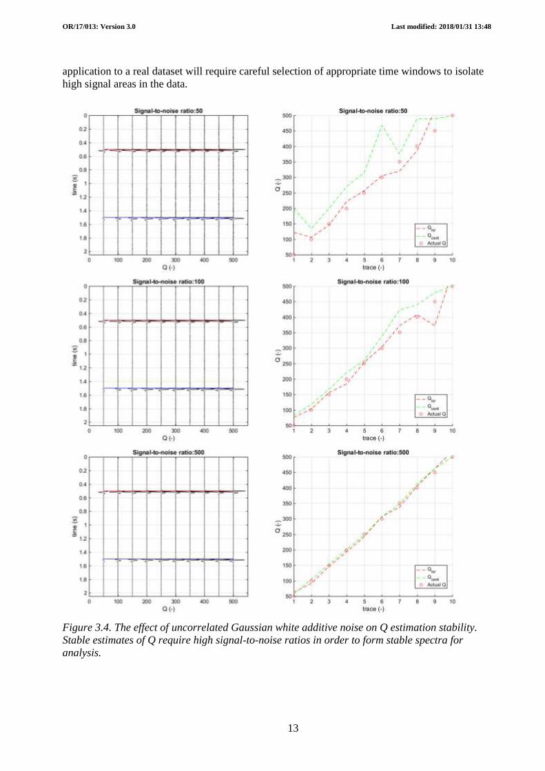
Both Q estimation techniques are highly sensitive to random noise however (Figure 3.4). It is

clear that stable estimates of Q require high signal-to-noise ratios (SNR), which means that


13

application to a real dataset will require careful selection of appropriate time windows to isolate

high signal areas in the data.

Figure 3.4. The effect of uncorrelated Gaussian white additive noise on Q estimation stability.

Stable estimates of Q require high signal-to-noise ratios in order to form stable spectra for

analysis.


14

3.6.2 Real data example

In order to demonstrate the workflow for Q estimation from stacked seismic data, a single inline

from the 1999 Sleipner repeat seismic survey was analysed using a combination of the techniques

described above. The seismic section (Figure 3.5) shows rather noisy traces, with the brightest

reflections occurring in the CO2 plume between traces 200 and 300. Scattered high amplitude

reflections between 0.6 and .0.8 s travel time correspond to methane accumulations in the

caprock.

Q analysis of the post-stack Sleipner data proved particularly challenging and was complicated by

a number of factors:

1. Wavelet interference.

2. Energy from reflection multiples contaminating the reference spectra used to calculate Q.

3. Shallow gas accumulations above the reservoir, which cause signal scattering and

attenuation in part of the data.

4. Time-dependent amplitude recovery applied during processing.

5. Deconvolution (spectral whitening) applied during processing.

6. Low SNR.

The SNR for each trace is plotted below the seismic section (Figure 3.5). The signal power was

computed from the zero lag of the cross-correlation between neighbouring traces, while noise

power was estimated from the zero lag of the average auto-correlation of the two traces, minus the

signal estimate. This technique assumes that the signal component is the same between adjacent

traces and the noise component is different and random. The mean SNR for the entire seismic line

is around 12, with higher values approaching 30 in the vicinity of the CO2 plume. Synthetic tests

suggest that the data are not suitable for robust Q estimation (Figure 3.4), although it might be

possible to achieve a meaningful measure of attenuation by carefully selecting suitable traces for

analysis.

For this example, Q was estimated from the final stacked and migrated seismic data using

frequency spectra extracted in narrow time windows about a reflection from close to the top of the

Utsira Sand reservoir (Figure 3.5) and about a high amplitude regional reflector some distance

below the Utsira reservoir (Figure 3.5). A narrow time window was essential for two reasons:

1. The low Signal-to-Noise Ratio (SNR) and lack of reflectivity at reservoir level means

that reliable Q estimates require careful selection of appropriate time windows to

isolate high signal areas in the data.

2. The CO2 is trapped beneath a low permeability mudstone close to the top of the

reservoir, so spectra used for Q estimation need to be selected from a short time

window about this reflection.

To this end, the SPWVD time-frequency distribution described above was used to calculate

frequency spectra. Q values were then calculated for traces 30, 273 and 480 (Figure 3.5) selected

on the basis of SNR and observed reflection strength (Figures 3.6 to 3.8).


15

Figure 3.5. Seismic inline from the 1999 Sleipner monitor survey, showing the reflective CO2

plume in the central part of the section. One reflector close to the top of the Utsira Sand (red line)

and one some distance below the Utsira Sand (blue) were used to estimate Q with analysed traces

shown as red wiggle traces. Lower panel shows a signal-to-noise estimate computed on a trace-

by-trace basis. The mean signal-to-noise ratio is around 12.


16

Figure 3.6. Q analysis of Trace 30 on the seismic section in Figure 3.5, outside the CO2 plume.

(a) The extracted seismic trace. (b) Time-frequency decomposition using the SPWVD. (c)

Smoothed frequency spectra extracted from the data. (d) Log spectral ratio plot showing the

straight line fit used to calculate Q. Red and blue stippled lines in (a), (b) and (c) show the time

picks used in the Q analysis.


17

Figure 3.7. Q analysis of Trace 273 on the seismic section in Figure 3.5, located within the CO2

plume. (a) The extracted seismic trace. (b) Time-frequency decomposition using the SPWVD. (c)


straight line fit used to calculate Q. Red and blue stippled lines in (a), (b)and (c) show the time



18

Figure 3.8. Q analysis of Trace 480 on the seismic section in Figure 3.5, from outside the CO2

plume. (a) The extracted seismic trace. (b) Time-frequency decomposition using the SPWVD. (c)


straight line fit used to calculate Q. Red and blue stippled lines in (a), (b) and (c) show the time


Calculated Q values (Table 3.1) can be compared with laboratory measurements on an Utsira

Sand core sample made by Falcon-Suarez et al. (2018) as part of DISECCS. They found that the

P-wave attenuation (1/QP) in partially saturated rock increased from 0.02 - 0.03 (Q = 50 - 32) in

brine saturated rock to around 0.06 - 0.08 (Q = 17 - 12.5). New rock physics relationships

proposed by Falcon-Suarez et al. (2018) indicate that at higher CO2 saturations (80% and above)

Q values would be in the range 20-30. There is therefore a degree of agreement on these figures.

Traces 30 and 480, through the brine-filled reservoir, have high Q values, similar to the laboratory

measurements. Trace 273, through the CO2 plume has lower Q values, but consistent with

generally quite high CO2 saturations.


19

Trace QLSR QPFS QMEAN 1/QMEAN

30 56.97 66.00 61.45 0.0163 273 19.26 28.00 23.63 0.0423 480 51.35 55.00 53.18 0.0188

Table 3.1. Results of Q analysis on selected traces extracted from the seismic line in Figure . LSR

log spectral ratio; PFS peak frequency shift.

Automated analysis of the entire seismic section proved less successful, with many traces giving

highly unstable Q estimates. It might be possible to improve the results by re-processing selected

traces using a scheme designed to more accurately preserve amplitude information inherent in the

signal. Noise could potentially be attenuated by forming “super-gathers” of adjacent common

midpoint bins.

3.7 REFERENCES

Falcon-Suarez, I., Papageorgiou, G., Chadwick, A., North, L., Best, A. & Chapman, M. 2018.

CO2-brine flow-through on an Utsira Sand core sample: experimental and modelling. Implications

for the Sleipner storage field. International Journal of Greenhouse Gas Control, 68 (2018), 236-

246.

Zhang, C. & Ulrychz, T.J., 2002. Estimation of quality factors from CMP records. Geophysics

1542–1547.


20

4 Fracture properties from seismic coda analysis

4.1 BACKGROUND

The occurrence and characteristics of fracturing in reservoirs and overburdens is a key storage

performance issue. Multi-component seismic data are typically used to characterise structural

anisotropy, but a logistically simpler approach involves the use of conventional 3D or multi-

azimuth 2D datasets. As a seismic wave propagates through the fractured medium the wavelet is

lengthened by a reverberating or ringing ‘coda’ or tail. Coda development is most pronounced

where the direction of propagation is parallel to the fracture system. So in principle the fracture

direction can be determined by analysing the length of the ringing ‘coda’ for seismic lines

acquired along different azimuths.

4.2 THEORY

Willis et al. (2006) described an algorithm to extract fracture distribution and orientation from

scattered seismic coda, where the fracture spacing is of a comparable dimension to the wavelength

of the seismic wavelet. Their algorithm was based on synthetic seismic models of a simple

reservoir comprising five layers of homogenous isotropic elastic media. A series of anisotropic

vertical fractures were introduced in the third layer of the model and assigned an elastic stiffness

of 8 x 108 Pa m

-1, to represent gas-filled fractures. Synthetic shot records were generated for a

series of models with fractures spaced at 10, 25, 35, 50 and 100 metres.

It was found that reflections beneath the fracture zone exhibited a ringing coda caused by

reverberations in the fractured zone. However a shot record acquired normal to the fracture

direction had little coherent energy below the top of the fractured zone, whereas shot records

acquired parallel to the fractures showed coherent reflections from below the top fractured zone

reflection. Consequently, the strike of the fracture zone could be identified using stacked NMO-

corrected azimuthal gathers.

In order to apply coda analysis to real datasets, the authors computed a transfer function by

deconvolving the autocorrelation function computed in a window above the fractured zone from

the autocorrelation function computed in a window below the fractured zone, using the Wiener-

Levinson algorithm. A clean spike or pulsed transfer function indicates no scattering, whereas a

long, ringing, transfer function is indicative of scattering within the zone between the two analysis

windows. The transfer functions from traces stacked in the direction parallel to fractures exhibited

more ringing than those in the direction perpendicular to fractures, albeit with transfer functions

showing very little change in shape until they were within 10° of the fracture strike direction on

the synthetic test examples.

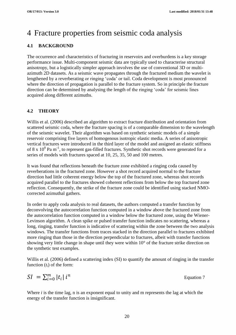
Willis et al. (2006) defined a scattering index (SI) to quantify the amount of ringing in the transfer

function (ti) of the form:

Where i is the time lag, n is an exponent equal to unity and m represents the lag at which the

energy of the transfer function is insignificant.

𝑆𝐼 = |𝑡𝑖|𝑚𝑖=0 𝑖𝑛 Equation 7


21

The scattering index is largest in the fracture-parallel direction. The program dsucoda computes

this scattering index for seismic traces in CWPSU format.

4.3 ALGORITHM

1. Read the CWPSU formatted seismic trace data and window about two time picks above

and below the zone of interest.

2. Compute the autocorrelations of the windowed trace data.

3. Form the transfer function using the Wiener-Levinson deconvolution algorithm (Levinson

recursion to solve the Toeplitz matrix).

4. Output the resulting transfer function in CWPSU trace format.

5. Compute the scattering index using Equation 7.

4.4 IMPLEMENTATION

The scattering index described above can be computed using dsucoda, which is contained in the

coda directory of the DiSECCS toolbox. It has been implemented in ANSI C as a plug-in to the

freely available Seismic Unix seismic data processing toolkit

(http://www.cwp.mines.edu/cwpcodes/).

4.5 EXAMPLE USAGE

Willis et al. (2006) presented an example of coda analysis applied to a 3D seismic survey acquired

over a fractured carbonate hydrocarbon reservoir (the Emilio field) in the central part of the

Adriatic Sea, near the eastern coast of Italy. This technique clearly has the potential to enhance

seismic monitoring of fractured CO2 storage reservoirs.

4.6 REFERENCES

Willis, M.E., D.R. Burns, R. Rao, B. Minsley, M.N. Toksöz & L.Vetri. 2006. Spatial Orientation

and Distribution of Reservoir Fractures from Scattered Seismic Energy. Geophysics 71 (5): O43.

doi:10.1190/1.2235977.



22

5 Spectral inversion

5.1 BACKGROUND

Spectral inversion is a technique that uses spectral decomposition to improve characterisation of

layers below the seismic tuning thickness. Absolute temporal layer thickness can be determined

together with the reflection coefficients of the upper and lower layer interfaces which can be used

to constrain layer velocity.

5.2 THEORY

The spectral inversion technique contained in the DiSECCS toolbox uses an inversion algorithm

formulated in the frequency domain. The method for two reflections is based on the constant

periodicity of the amplitude spectrum for a single layer of thickness T. The cost function is

defined by Puryear & Castagna (2008) as:

It is evaluated across a range of frequencies. 𝐺(𝑓) is the magnitude of the amplitude spectrum and

𝑘 = 𝑟𝑒2 − 𝑟𝑜

2 where 𝑟𝑜 and 𝑟𝑒 are the odd and even components of the reflection coefficient pair.

Finding the global minimum of the cost function by scanning a reasonable model space in T and k

gives the desired solution for T and k. The remaining parameters are then calculated from:

And

5.3 ALGORITHM

1. Read in the seismic trace and source wavelet and transform both trace and wavelet into the

frequency domain.

2. Calculate the normalised amplitude of the input trace at discrete frequency values.

3. Calculate the gradient of the amplitude distribution in the frequency domain.

4. Estimate the cost function across a suitable frequency range to determine the temporal

thickness of the layer, T, and k.

5. Loop through the selected frequency range and derive the odd and even components of the

reflection amplitude pair.

6. Output results.

5.4 IMPLEMENTATION

𝑐𝑜𝑠𝑡 𝑓𝑢𝑛𝑐𝑡𝑖𝑜𝑛 = 𝐺(𝑓)𝑑𝐺(𝑓)

𝑑𝑓+ 2𝜋𝑇𝑘 sin(2𝜋𝑓𝑇) Equation 8

𝑟𝑜 = 𝐺(𝑓)2

4− 𝑘(cos(𝜋𝑓𝑇) )2 Equation 9

𝑟𝑒 = 𝑘 − 𝑟𝑜2 Equation 10


23

The spectral inversion algorithm described above has been implemented in the ANSI C code

dsuspecinv2, which is included in the specdecomp directory of the DiSECCS toolbox. This is a

plug-in to the freely available Seismic Unix seismic data processing toolkit

(http://www.cwp.mines.edu/cwpcodes/) and the input data comprise seismic trace(s) in CWPSU

format. Output from the code consists of two text files containing the calculated reflectivity

response and the evaluated cost function. Note that dsuspecinv2 uses the Fast Fourier Transform

package FFTW3 which can be downloaded from www.fftw.org.

5.5 EXAMPLE USAGE

5.5.1 Synthetic example

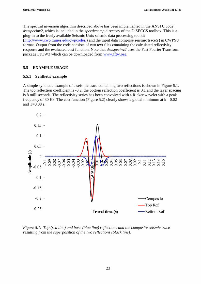
A simple synthetic example of a seismic trace containing two reflections is shown in Figure 5.1.

The top reflection coefficient is -0.2, the bottom reflection coefficient is 0.1 and the layer spacing

is 8 milliseconds. The reflectivity series has been convolved with a Ricker wavelet with a peak

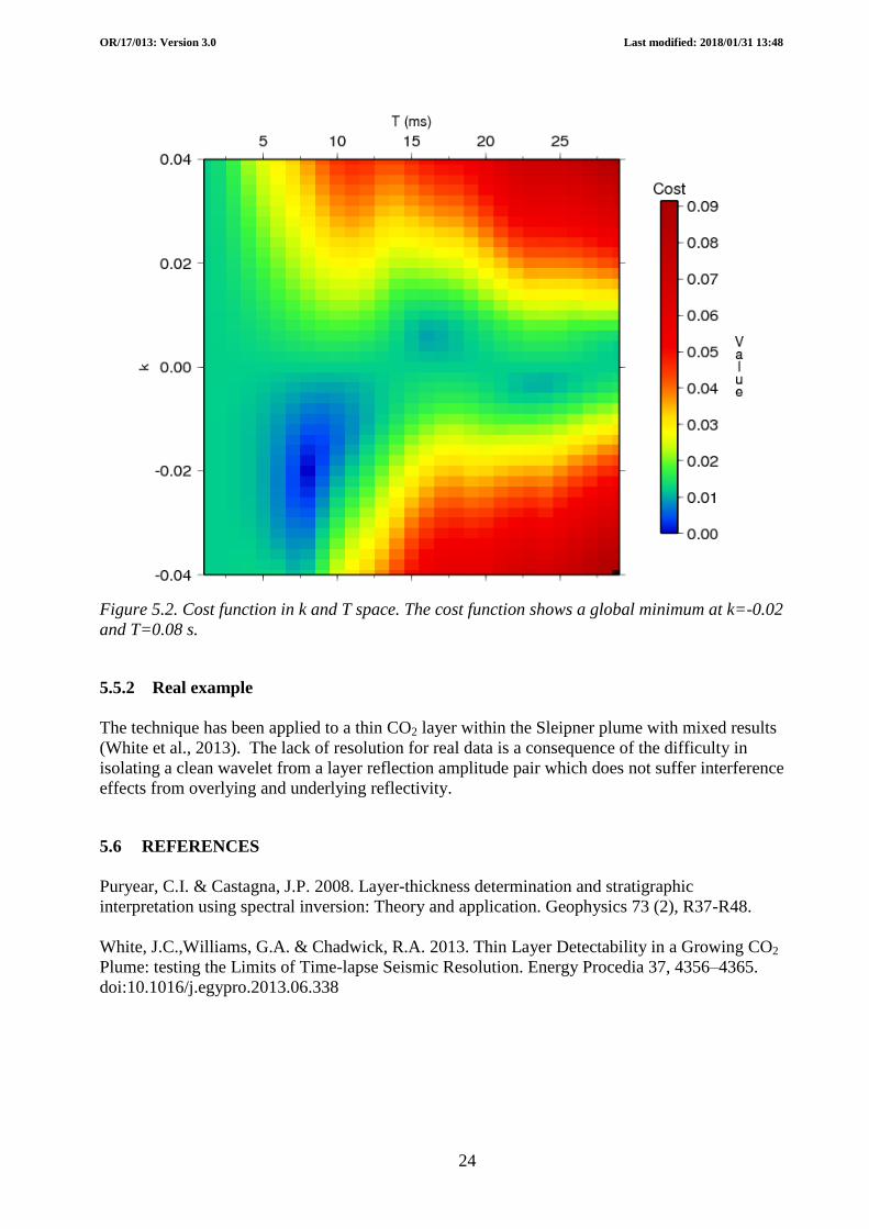
frequency of 30 Hz. The cost function (Figure 5.2) clearly shows a global minimum at k=-0.02

and T=0.08 s.

Figure 5.1. Top (red line) and base (blue line) reflections and the composite seismic trace

resulting from the superposition of the two reflections (black line).


http://www.fftw.org/


24

Figure 5.2. Cost function in k and T space. The cost function shows a global minimum at k=-0.02

and T=0.08 s.

5.5.2 Real example

The technique has been applied to a thin CO2 layer within the Sleipner plume with mixed results

(White et al., 2013). The lack of resolution for real data is a consequence of the difficulty in

isolating a clean wavelet from a layer reflection amplitude pair which does not suffer interference

effects from overlying and underlying reflectivity.

5.6 REFERENCES

Puryear, C.I. & Castagna, J.P. 2008. Layer-thickness determination and stratigraphic

interpretation using spectral inversion: Theory and application. Geophysics 73 (2), R37-R48.

White, J.C.,Williams, G.A. & Chadwick, R.A. 2013. Thin Layer Detectability in a Growing CO2

Plume: testing the Limits of Time-lapse Seismic Resolution. Energy Procedia 37, 4356–4365.

doi:10.1016/j.egypro.2013.06.338


25

6 Rock Physics Models

6.1 BACKGROUND

Robust interpretation and analysis of seismic datasets must be underpinned by good

understanding of the physical processes that govern the seismic properties of reservoir rock as

fluid and stress distributions change.

6.2 IMPLEMENTATION

The rock physics models are implemented as a Mathematica note book

(DiSECCS_rock_physics_models.nb) included in the .mathematica directory of the DiSECCS

toolbox. A free viewer can be downloaded from the URL: http://www.wolfram.com/cdf-player

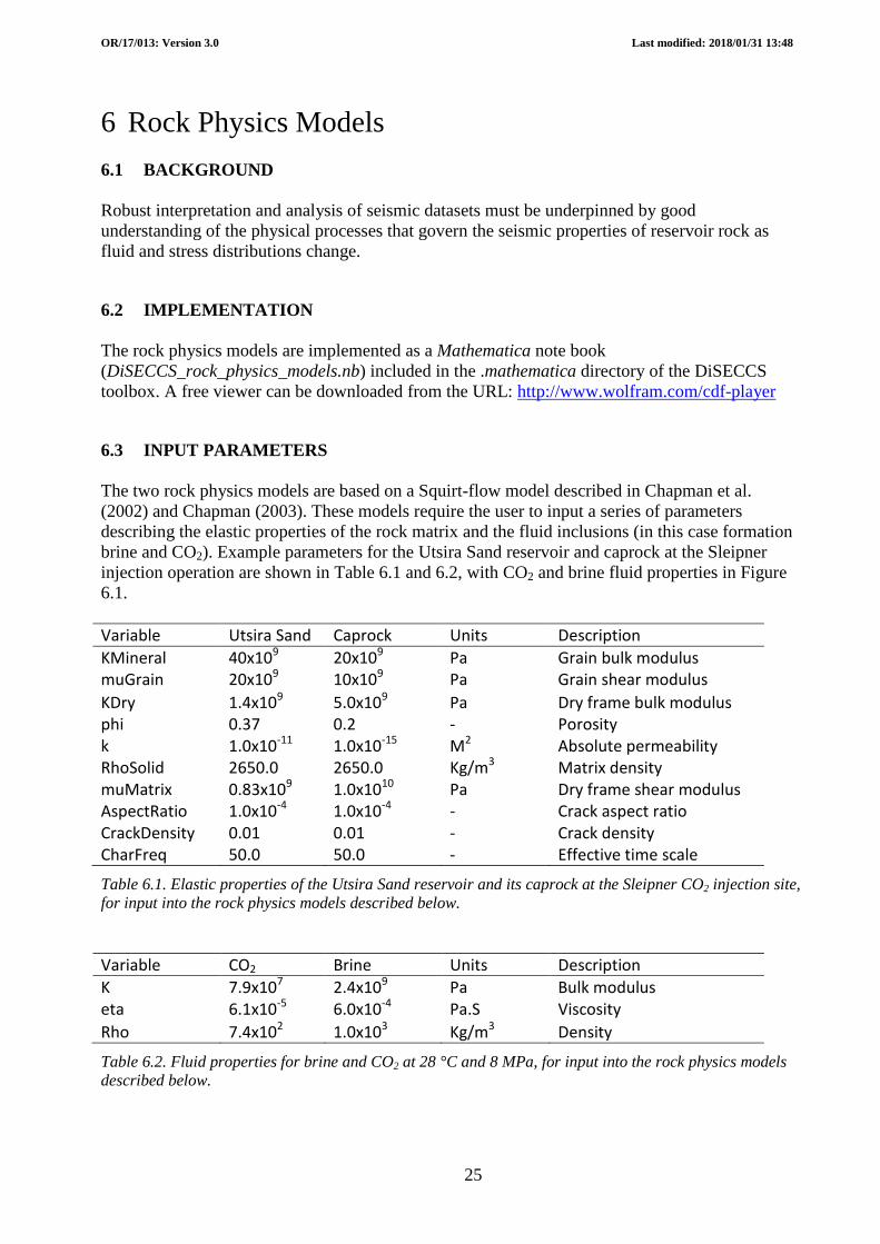
6.3 INPUT PARAMETERS

The two rock physics models are based on a Squirt-flow model described in Chapman et al.

(2002) and Chapman (2003). These models require the user to input a series of parameters

describing the elastic properties of the rock matrix and the fluid inclusions (in this case formation

brine and CO2). Example parameters for the Utsira Sand reservoir and caprock at the Sleipner

injection operation are shown in Table 6.1 and 6.2, with CO2 and brine fluid properties in Figure

6.1.

Variable Utsira Sand Caprock Units Description

KMineral 40x109 20x109 Pa Grain bulk modulus muGrain 20x109 10x109 Pa Grain shear modulus

KDry 1.4x109 5.0x109 Pa Dry frame bulk modulus phi 0.37 0.2 - Porosity k 1.0x10-11 1.0x10-15 M2 Absolute permeability RhoSolid 2650.0 2650.0 Kg/m3 Matrix density muMatrix 0.83x109 1.0x1010 Pa Dry frame shear modulus AspectRatio 1.0x10-4 1.0x10-4 - Crack aspect ratio CrackDensity 0.01 0.01 - Crack density CharFreq 50.0 50.0 - Effective time scale

Table 6.1. Elastic properties of the Utsira Sand reservoir and its caprock at the Sleipner CO2 injection site,

for input into the rock physics models described below.

Variable CO2 Brine Units Description

K 7.9x107 2.4x109 Pa Bulk modulus eta 6.1x10-5 6.0x10-4 Pa.S Viscosity

Rho 7.4x102 1.0x103 Kg/m3 Density

Table 6.2. Fluid properties for brine and CO2 at 28 °C and 8 MPa, for input into the rock physics models

described below.

http://www.wolfram.com/cdf-player


26

Figure 6.1. Fluid properties for CO2 and brine (w) at a pressure of 8 MPa. (a) Density ρ; (b) bulk

modulus K and (c) viscosity η.

6.4 DETERMINING EFFECTIVE FLUID MODULUS IN A CRACKED POROUS

MEDIUM

The algorithms are based on a Squirt-flow model described in Chapman et al. (2002), Chapman

(2003) and Papageorgiou & Chapman (2015), in which the grains of a porous material are

themselves allowed to have porosity in the form of micro-cracks. The effective fluid moduli are

computed by assuming that fluids are distributed between pores (Sp) and cracks (Sc) in the rock:


27

Where Sw is the water saturation, S0 is a critical saturation parameter and cf is given by:

Where ε is the crack density and r the aspect ratio of the cracks. The cracks are modelled as coin-

like ellipsoidal inclusions with a crack density (ε) given by ε=3φc

4πr where φc is the volume

fraction of cracks in the effective medium.

Pores and cracks are assigned different fluid moduli in the model as illustrated by the example

pseudocode (Box 6.1). This formulation incorporates hysteresis effects, as the spatial distribution

of fluids between cracks and pores will be different during imbibition and drainage (see

Papageorgiou & Chapman 2015 for a detailed explanation).

Box 6.1. Pseudo-code showing calculation of effective fluid moduli for use in the rock physics models

described below. Input parameters are shown in red and are defined in Table 6.1 and 6.2. Output

parameters are highlighted in blue.

6.5 THE EFFECT OF CAPILLARY PRESSURE ON THE EFFECTIVE FLUID

MODULUS

Equation 11

Equation 12

/* input */

Phi /*porosity */

AspectRatio /* crack aspect ratio */

CrackDensity /* crack density */

waterModulus /* brine bulk modulus */

gasModulus /* CO2 bulk modulus */

/* calculate crack fraction */

crackFraction=(4/3*pi*CrackDensity*AspectRatio)

/(4/3*pi*CrackDensity*AspectRatio + phi)

/* calculate relative saturations */

If (0 < Sw < S0)

Sp=Sw((1-cf/S0)/1-cf))

Sc=Sw/S0

Else If (S0 < Sw < 1)

Sp=(Sw -cf)/1-cf)

Sc=1

/* Output fluid moduli for pores and cracks */

CrackFluidModulus=1(Sc/waterModulus+1-Sc)/gasModulus)

PoreFluidModulus=1(Sp/waterModulus+1-Sp)/gasModulus)


28

Papageorgiou et al. (2016) incorporated capillary pressure effects into their calculations of the

effective fluid modulus by including a capillary pressure parameter q which relates the wetting

and non-wetting phase fluid pressures:

Where PCO2 is the CO2 (non-wetting phase) pressure, Pw the brine (wetting phase) pressure, KCO2

the CO2 bulk modulus, and KW the brine bulk modulus.

The effective fluid modulus (Kf) is then calculated by:

Where SW is the brine saturation.

Example pseudocode used to calculate Kf is shown in Box 6.26.2, while Figure 6.2 shows the

effect on fluid bulk modulus of varying the parameter q.

Box 6.2. Pseudo-code showing calculation of effective fluid moduli incorporating capillary pressure effects

for use in rock physics model 2 described below. Input parameters are shown in red and are defined in

Table 6.1 and Table 6.2. Output parameters are highlighted in blue.

Figure 6.2. The effect of varying the capillary pressure parameter q on the effective fluid modulus (Kf).

Equation 13

Equation 14

/* input */

Sw /*water saturation */

waterModulus /* brine bulk modulus */

gasModulus /* CO2 bulk modulus */

q /* the q factor */

/* Output fluid modulus */

FluidModulus=…

(Sw (1-q)+q)/(Sw/waterModulus+q*(1-Sw)/gasModulus)


29

6.6 THE EFFECTIVE TIMESCALE PARAMETER

Squirt-flow models introduce stiffening in the saturated rock matrix, based on a relaxation

mechanism whose characteristic frequency depends on fluid content as well as rock matrix

parameters. Chapman (2003) showed that fluid mobility is the key parameter affecting the

characteristic time scale of this process, a fact that has been verified experimentally many times.

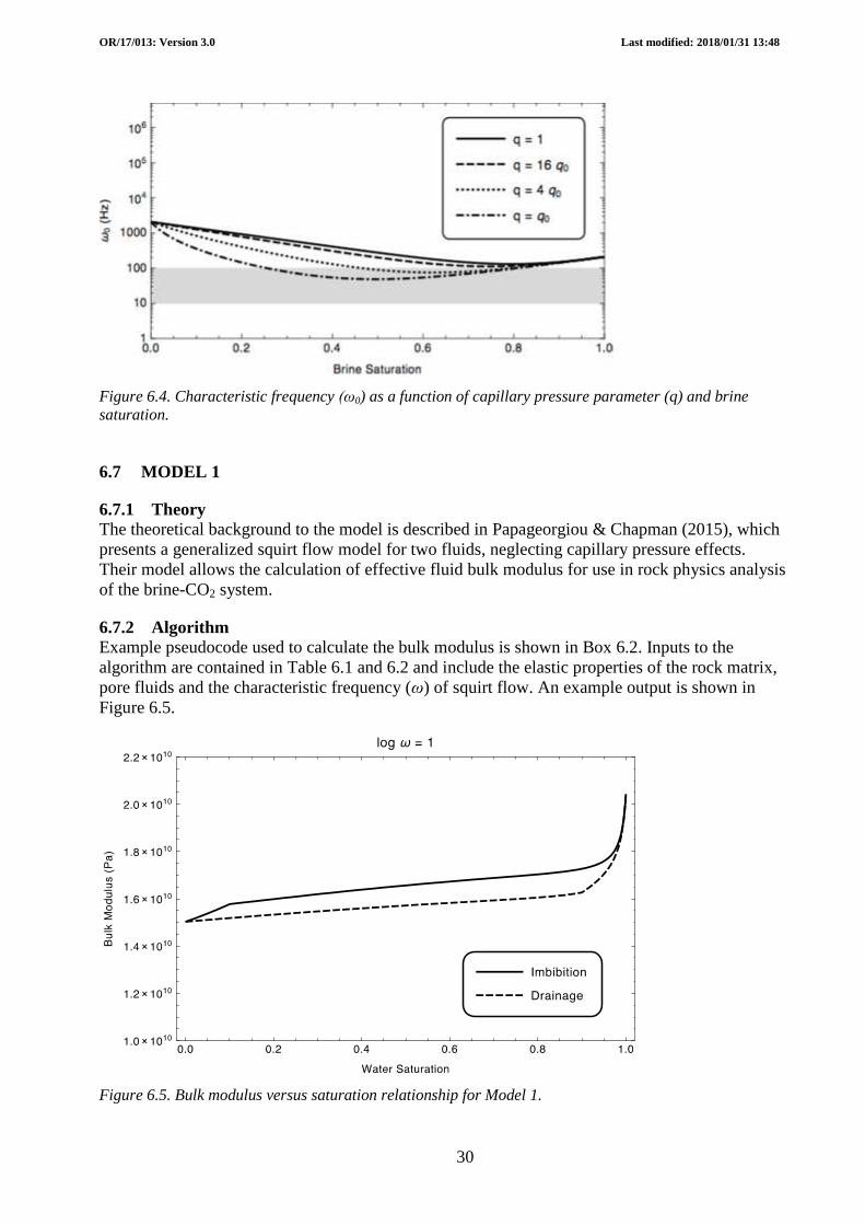
The characteristic frequency (ω) of squirt flow is given by:

Where τ is the characteristic time scale, the coefficient B is a function of various rock properties

(around 50 Pa for the Utsira Sand), SW is the water saturation, q as described above and k/η is the

mobility of the effective fluid phase (relative phase permeability / phase viscosity).

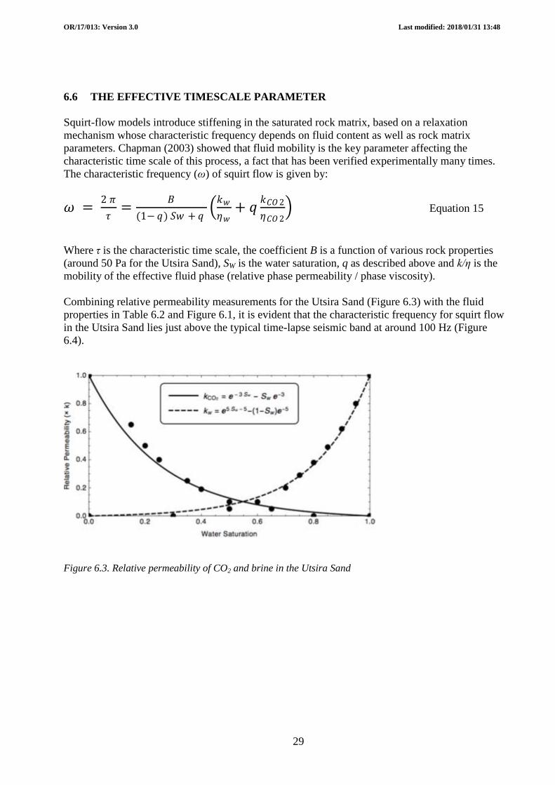
Combining relative permeability measurements for the Utsira Sand (Figure 6.3) with the fluid

properties in Table 6.2 and Figure 6.1, it is evident that the characteristic frequency for squirt flow

in the Utsira Sand lies just above the typical time-lapse seismic band at around 100 Hz (Figure

6.4).

Figure 6.3. Relative permeability of CO2 and brine in the Utsira Sand

𝜔 = 2 𝜋

𝜏=

𝛣

(1− 𝑞) 𝑆𝑤 + 𝑞 𝑘𝑤

𝜂𝑤+ 𝑞

𝑘𝐶𝑂2

𝜂𝐶𝑂2 Equation 15


30

Figure 6.4. Characteristic frequency (ω0) as a function of capillary pressure parameter (q) and brine

saturation.

6.7 MODEL 1

6.7.1 Theory

The theoretical background to the model is described in Papageorgiou & Chapman (2015), which

presents a generalized squirt flow model for two fluids, neglecting capillary pressure effects.

Their model allows the calculation of effective fluid bulk modulus for use in rock physics analysis

of the brine-CO2 system.

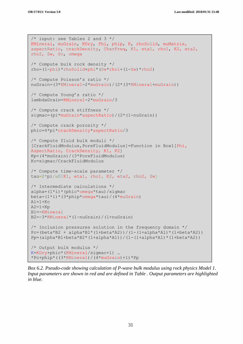
6.7.2 Algorithm

Example pseudocode used to calculate the bulk modulus is shown in Box 6.2. Inputs to the

algorithm are contained in Table 6.1 and 6.2 and include the elastic properties of the rock matrix,

pore fluids and the characteristic frequency (ω) of squirt flow. An example output is shown in

Figure 6.5.

Figure 6.5. Bulk modulus versus saturation relationship for Model 1.


31

Box 6.2. Pseudo-code showing calculation of P-wave bulk modulus using rock physics Model 1.

Input parameters are shown in red and are defined in Table . Output parameters are highlighted

in blue.

/* input: see Tables 2 and 3 */

KMineral, muGrain, KDry, Phi, phip, K, rhoSolid, muMatrix,

aspectRatio, crackDensity, CharFreq, K1, eta1, rho1, K2, eta2,

rho2, Sw, Sc, omega

/* Compute bulk rock density */

rho=(1-phi)*rhoSolid+phi*(Sw*rho1+(1-Sw)*rho2)

/* Compute Poisson’s ratio */

nuGrain=(3*KMineral-2*muGrain)/(2*(3*KMineral+muGrain))

/* Compute Young’s ratio */

lambdaGrain=KMineral-2*muGrain/3

/* Compute crack stiffness */

sigmac=(pi*muGrain*aspectRatio)/(2*(1-nuGrain))

/* Compute crack porosity */

phic=4*pi*crackDensity*aspectRatio/3

/* Compute fluid bulk moduli */

[CrackFluidModulus,PoreFluidModulus]=Function in Box1[Phi,

AspectRatio, CrackDensity, K1, K2]

Kp=(4*muGrain)/(3*PoreFluidModulus)

Kc=sigmac/CrackFluidModulus

/* Compute time-scale parameter */

tau=2*pi/ω0[K1, eta1, rho1, K2, eta2, rho2, Sw]

/* Intermediate calculations */

alpha=(1*i)*(phic*omega*tau)/sigmac

beta=(1*i)*(3*phip*omega*tau)/(4*muGrain)

A1=1+Kc

A2=1+Kp

B1=-KMineral

B2=-3*KMineral*(1-nuGrain)/(1+nuGrain)

/* Inclusion pressures solution in the frequency domain */

Pc=(beta*B2 + alpha*B1*(1+beta*A2))/(1-(1+alpha*A1)*(1+beta*A2))

Pp=(alpha*B1+beta*B2*(1+alpha*A1))/(1-(1+alpha*A1)*(1+beta*A2))

/* Output bulk modulus */

K=KDry+phic*(KMineral/sigmac+1) …

*Pc+phip*((3*KMineral)/(4*muGrain)+1)*Pp


32

6.8 MODEL 2

6.8.1 Theory

The background to the model is described in Papageorgiou et al. (2016), which presents a

theoretical derivation of a Brie-like fluid mixing law by incorporating a capillary pressure term

into the inclusion-based model described above (see also Papageorgiou & Chapman 2015). The

inclusions are saturated by multiple fluids.

6.8.2 Algorithm

Example pseudocode used to calculate the bulk modulus is shown in Box . Inputs to the algorithm

are contained in Table 6.1 and 6.2. An example output is shown in Figure 6.6.

Figure 6.6. P-wave velocity (top) and attenuation (bottom) versus saturation relationship for Model 2 in

the case of supercritical CO2 (left) and liquid CO2 (right) across different frequency ranges (ω).


33

Box 6.4. Pseudo-code showing calculation of P-wave bulk modulus using rock physics Model 2.

Input parameters are shown in red and are defined in Table 6.1 and 6.2. Output parameters are

highlighted in blue.

/* input: see Tables 2 and 3 */

KMineral, muGrain, KDry, Phi, phip, K, rhoSolid, muMatrix,

aspectRatio, crackDensity, CharFreq, K1, eta1, rho1, K2, eta2,

rho2, Sw, Sc, omega

/* Compute bulk rock density */

rho=(1-phi)*rhoSolid+phi*(Sw*rho1+(1-Sw)*rho2)

/* Compute Poisson’s ratio */

nuGrain=(3*KMineral-2*muGrain)/(2*(3*KMineral+muGrain))

/* Compute Young’s ratio */

lambdaGrain=KMineral-2*muGrain/3

/* Compute crack stiffness */

sigmac=(pi*muGrain*aspectRatio)/(2*(1-nuGrain))

/* Compute crack porosity */

phic=4*pi*crackDensity*aspectRatio/3

/* Compute fluid bulk moduli */

[FluidBulkModulus]=Function in Box2[Sw, K1, K2, q]

Kp=(4*muGrain)/(3*FluidBulkModulus)

Kc=sigmac/FluidBulkModulus

/* Compute time-scale parameter */

tau=2*pi/ω0[K1, eta1, rho1, K2, eta2, rho2, Sw]

/* Intermediate calculations */

alpha=(1*i)*(phic*omega*tau)/sigmac

beta=(1*i)*(3*phip*omega*tau)/(4*muGrain)

A1=1+Kc

A2=1+Kp

B1=-KMineral

B2=-3*KMineral*(1-nuGrain)/(1+nuGrain)

/* Inclusion pressures solution in the frequency domain */

Pc=(beta*B2 + alpha*B1*(1+beta*A2))/(1-(1+alpha*A1)*(1+beta*A2))

Pp=(alpha*B1+beta*B2*(1+alpha*A1))/(1-(1+alpha*A1)*(1+beta*A2))

/* Output bulk modulus */

K=KDry+phic*(KMineral/sigmac+1) …

*Pc+phip*((3*KMineral)/(4*muGrain)+1)*Pp


34

6.9 REFERENCES

Chapman, M. 2003. Frequency-Dependent Anisotropy due to Meso-Scale Fractures in the

Presence of Equant Porosity. Geophysical Prospecting 51 (5): 369–79. doi:10.1046/j.1365-

2478.2003.00384.x.

Chapman, Mk, S. V. Zatsepin & S. Crampin. 2002. Derivation of a Microstructural Poroelastic

Model. Geophysical Journal International 151 (2): 427–51. doi:10.1046/j.1365-

246X.2002.01769.x.

Papageorgiou, G. & M. Chapman. 2015. Multifluid Squirt Flow and Hysteresis Effects on the

Bulk Modulus–water Saturation Relationship. Geophysical Journal International 203 (2): 814–17.

doi:10.1093/gji/ggv333.

Papageorgiou, G., K. Amalokwu & M. Chapman. 2016. Theoretical Derivation of a Brie-like

Fluid Mixing Law. Geophysical Prospecting 64 (4): 1048–53. doi:10.1111/1365-2478.12380.


35

7 Rock physics laboratory measurements

7.1 BACKGROUND

Direct measurement of rock samples in the laboratory provides the means of calibrating and

verifying rock physics models such as those described above. Experimental work in DiSECCS

focussed on unconsolidated sands such as are found at Sleipner and on synthetic rocks where

properties in terms of porosity and permeability can to some extent be controlled.

7.2 METHODOLOGY

The experimental methodology can be found in the DiSECCS WP1 - 4 final report, with details of

the experimental rig in Falcon-Suarez et al. (2014, 2016,2018).

7.3 RESULTS

An EXCEL spreadsheet containing measurements on a number of different samples, of P- and S-

wave velocity, seismic attenuation and electrical resistivity are included in the spreadsheets

directory of the DiSECCS Seismic Unix toolbox. Complete datasets of the experimental work

developed during the project can be found on the UKCCSRC archive:

http://www.bgs.ac.uk/ukccs/dataset.cfm?id=19877273

7.4 REFERENCES

Falcon-Suarez, I., North, L. & Best, A. 2014. Experimental Rig to Improve the Geophysical and

Geomechanical Understanding of CO2 Reservoirs. European Geosciences Union General

Assembly 2014, EGU Division Energy, Resources & the Environment (ERE) 59 (January): 75–

81. doi:10.1016/j.egypro.2014.10.351.

Falcon-Suarez, I., North, L., Amalokwu, K. & Best, A. 2016. Integrated Geophysical and

Hydromechanical Assessment for CO2 Storage: Shallow Low Permeable Reservoir Sandstones.

Geophysical Prospecting 64 (4): 828–47. doi:10.1111/1365-2478.12396.

Falcon-Suarez, I., Papageorgiou, G., Chadwick, A., North, L., Best, A. & Chapman, M. 2018.

CO2-brine flow-through on an Utsira Sand core sample: experimental and modelling. Implications

for the Sleipner storage field. International Journal of Greenhouse Gas Control, 68 (2018), 236-

246.

http://www.bgs.ac.uk/ukccs/dataset.cfm?id=19877273

Date post:	12-Mar-2022
Category:	Documents
Upload:	others
View:	1 times
Download:	0 times

DiSECCS - Diagnostic Seismic Toolbox for Efficient Control ...

Documents