Dispersion Models of Atmospheric Air Pollutants

University Bulletin – ISSUE No.18- Vol. (3) – August - 2016. - 56 -

Dispersion Models of Atmospheric Air Pollutants Dr. Ali Abusaloua, Ruqaia Sheliq, Chemical Engineering

Department , Faculty of Engineering- Sabrata zawia University

Abstract: Air quality models are typically used to predict the fate and transport

of air emissions from industrial sources to comply with environmental standards, as well as to determine pollution control requirements.

For many years, environmental protection agencies over the world used several gas dispersion based models in air quality impact assessment.

As an air pollutant is transported from a source to a potential receptor the pollutant disperses into the surrounding air so that it arrives at a much lower concentration than it was on leaving the source. Strict environmental regulations worldwide resulted in an ever growing concern about the validity and reliability of air quality dispersion models.

Due to the high performance of coding and flexibility in representation of output results which are available in MATLAB program.

Dr. Ali Abusaloua, Ruqaia Sheliq ـــــــــــــــــــــــــــــــــــــــــــــــــــــــــــــــــــــــــــــــــــــــــــــــــــــ


The MATLAB code was developed for Gauss dispersion model of air pollutants by using scripts and built in functions to simulate the effect of several parameters in downwind emission of gas pollutants. Keywords: Air pollution; Dispersion of Air Pollutants; Gaussian plume model 1. Introduction:

The importance of natural gas coming from its use considered as a main fuel for both domestic and industrial purposes: Natural gas is used locally for domestic purposes by establishing or expanding gas distribution nets in towns; hence, it is used in houses for cooking and heating purposes, It is also used in central heating due to several advantages. However, natural gas doesn't need any storing and it is easy to get any amount [1, 2]. Natural Gas is used primarily as a fuel in Power Generation and as a raw material in Hydrogen Production, Vehicles, domestic use and Fertilizers.

Sources of air pollution are either man made or natural. Man-made sources are what it was focused on because it may be able to control some of these sources. Both gaseous and particulate sources are troublesome. Several environmental standards have been set in order to reduce or (immigrate) concentrations for these materials in the atmosphere and in the emissions from chimneys. The concentration and the flow rate of the emissions are information required to determine the downwind transport of the pollutants. Knowing the location of the source relative to the receptor would allow us to calculate the concentration at a particular downwind receptor using a dispersion model [3, 4].

Air pollution models are routinely used in environmental impact assessments, risk analysis and emergency planning, and source apportionment studies. The concentration of an air pollutant at a given

Dispersion Models of Atmospheric Air Pollutants ــــــــــــــــــــــــــــــــــــــــــــــــــــــــــــــــــــــ


place is a function of a number of variables, including the emission rate, the distance of the receptor from the source, and the atmospheric conditions. The most important atmospheric conditions are wind speed, wind direction, and the vertical temperature structure of the local atmosphere. If the temperature decreases with height at a rate higher than the adiabatic lapse rate, the atmosphere is in unstable equilibrium and vertical motions are enhanced [5, 6].

Atmospheric air quality dispersion models are usually used to estimate just how much reduction has occurred during the transport of pollutant from an industrial source, and consequently to project the pollution concentration at ground level. Dispersion models usually incorporate meteorological, terrain, physical and chemical characteristics of the effluent and source design to simulate the formation and transport of pollutant plumes[7, 8].

In this work, the influence of stack height, wind speed, earth's surface conditions, stability class of atmosphere were studied, by solving a model equations for ground level concentrations of pollutants. The MATLAB algorithm was developed using scripts and built in functions to simulate the effect of several parameters in downwind emission of gas pollutants . 2. Development of a dispersion model:

There are three general types of dispersion models: box, plume, and puff. A variation on the box model is the cell model. The box model is conceptually the simplest although some relatively complex models have been built on box model foundations. The plume and puff models are more involved and complex models have been constructed using these concepts. In the Gaussian plume dispersion model the concentration of pollution



downwind from a source is treated as spreading outward from the centerline of the plume following a normal statistical distribution. The constants of the distribution are determined by the stability of the atmosphere and the "roughness" or "smoothness" of the earth's surface [9]. 2.1 Principles of smoke-plume model:

The atmospheric temperature profile affects the dispersion of pollution from a smokestack, Five special models have been observed and classified by the following:

If a smokestack were to emit pollutants into a neutrally stable atmosphere, It might be expected the plume to be relatively symmetrical, the term used to describe this plume is coning; If the atmosphere is very unstable, and there is rapid vertical air movement, both up and down, producing a looping plume; if the stable atmosphere greatly restricts the dispersion of the plume in the vertical direction, although it still spreads horizontally, this result is called a fanning plume; if the emissions from a smokestack that is under an inversion layer head downward much more easily than upward, the resulting fumigation can lead to greatly elevated downwind, ground-level concentrations. When the stack is above an inversion layer, ,mixing in the upward direction is uninhibited, but downward motion is greatly restricted by the inversion's stable air. such lofting plumes are helpful in terms of exposure to people at ground level. Thus, a common approach to air pollution control has be built taller and taller stack to emit pollutants above inversions [10].

When the day is very sunny with some wind blowing, radiation from the ground upward is very good. Strong convection currents moving upward are produced. Under these conditions plumes tend to loop upwards and then down to the ground in what are called looping plumes.



When the day is dark with steady relatively strong winds, the temperature profile will be neutral so that the convection currents will be small. Under these conditions the plume will proceed downwind spreading in a cone shape. Hence the name coning plume is applied. Under these conditions dispersion should most readily be described by Gaussian models [11]. 2.1.1 Gaussian Plume Model:

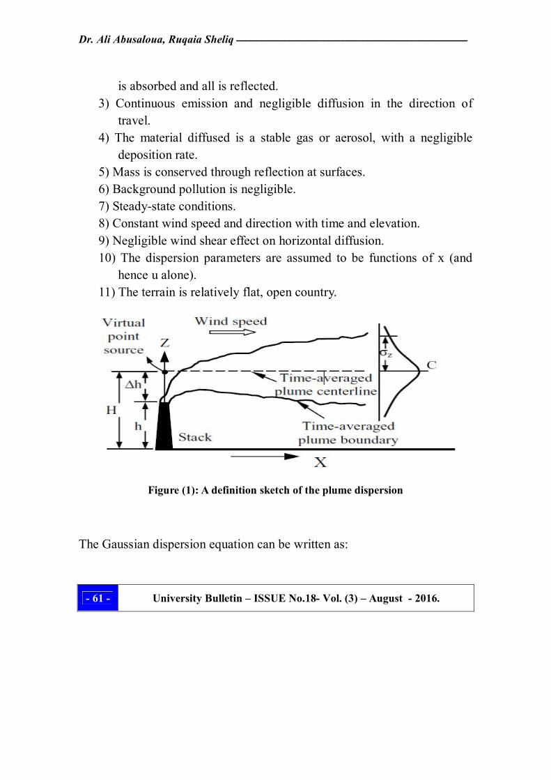
In the Gaussian plume dispersion model the concentration of pollution downwind from a source is treated as spreading outward from the centerline of the plume following a normal statistical distribution. The plume spreads in both the horizontal and vertical directions. In the model, determining the pollutant concentrations at ground-level beneath an elevated plume involves two main steps; first, the height to which the plume rises at a given downwind distance from the plume source is calculated. The calculated plume rise is added to the height of the plume's source point to obtain the so-called "effective stack height". Second, the ground-level pollutant concentration beneath the plume at the given downwind distance is predicted using the Gaussian dispersion equation. The Gaussian-point source dispersion equation relates to average steady-state pollutant concentrations to the source strength, wind speed, effective stack height and atmospheric conditions The plume spreads in both the horizontal and vertical directions, as illustrated in Figure (1). It is important to note the following assumptions that are incorporated into the analysis [12]:

1)- The rate of emissions from the source is constant. 2)- The pollutant is conservative; that is, it is not lost by decay,

chemical reaction, or deposition. When it hits the ground, none



is absorbed and all is reflected. 3) Continuous emission and negligible diffusion in the direction of

travel. 4) The material diffused is a stable gas or aerosol, with a negligible

deposition rate. 5) Mass is conserved through reflection at surfaces. 6) Background pollution is negligible. 7) Steady-state conditions. 8) Constant wind speed and direction with time and elevation. 9) Negligible wind shear effect on horizontal diffusion. 10) The dispersion parameters are assumed to be functions of x (and

hence u alone). 11) The terrain is relatively flat, open country.

Figure (1): A definition sketch of the plume dispersion

The Gaussian dispersion equation can be written as:



Where = concentration at ground-level at the point (x ,y), µg/m3 = distance directly downwind, m = horizontal distance from the plum center line, m Z= vertical direction, m = emission rate of pollutants, µg/s = effective stack height, m, ( = h + ∆h), where h = actual stack height, and ∆h=plume rise)

= average wind speed at the effective height of the stack, m/s σy= horizontal dispersion coefficient (standard deviation),m σ z = vertical dispersion coefficient (standard deviation),m

In this equation, the ground is usually assumed to be a perfect reflector and its presence is represented by a mirror image source placed below ground. Gaussian plume equation given here is less general than it can be, and applies only for (z=0) [13].

Plume rise Δh plays an important role in determining ground-level concentrations for real sources. Gaussian plume models are applicable for downwind distance, x>100 m, because near the source concentration approaches infinity. Accordingly, many researchers imposed a lower limit on σy(x) and σz(x), or an upper limit on the near source concentration. Gaussian plume models have been developed for point sources (e.g., stacks), line sources (e.g., roads), and area sources (e.g., spoil piles). The basic Gaussian plume model assumes a point source. Line sources can be approximated as a series of source points or a model that is specifically designed for line sources. Area sources can be approximated by assuming



the source is further away from the receptor than it actually is, such that the plume is already as wide as the area source at the correct distance.

Table 1: Atmospheric Stability Classifications Surface

wind speeda(m/s)

Day solar insolation Night cloudinesse

Strongb Moderatec Slightd Cloudy (≥4/8)

Clear (≤3/8)

<2 A A-Bf B E F 2-3 A-B B C E F 3-5 B B-C C D E 5-6 C C-D D D D >6 C D D D D

a Surface wind speed is measured at 10 m above the ground. b Corresponds to clear summer day with sun higher than 600 above the

horizon. c Corresponds to a summer day with a few broken clouds, or a clear day

with sun 35-600 above the horizon. d Corresponds to a fall afternoon, or a cloudy summer day, or clear

summer day with the sun 15-350 above the horizon. e Cloudiness is defined as the fraction of sky covered by clouds. F For A-B, B-C, or C-D conditions, average the values obtained for

each. Note: A, Very unstable; B, moderately unstable; C, slightly unstable;

D, neutral; E, slightly stable; F, stable. Regardless of wind speed, class D should be assumed for overcast conditions, day or night [14].

In order to use Eq. (1) in practical applications, It is required to know the dispersion coefficients σy and σz. These will be functions of downwind distance x and will also be unequal, since the characteristic turbulence velocities are expected to be different in the horizontal and vertical



directions. Finally, They are expected to be depends on atmospheric conditions: for stable conditions, the r.m.s. velocities are very low and hence the dispersion coefficients small; for unstable conditions, the turbulence is vigorous and we expect much larger dispersion coefficients. The σ’s can be estimated at a given downwind distance from the following equations and hence Eq. (1) can be applied to give the mean pollutant: σy = a x0.894

-------------------→ (2)

σz = c xd + f -------------------→ (3) Where the constant , , , and f are given in Table(2) for each stability classification. The downwind distance must be expressed in kilometres to yield and

in kilometers

Table 2: Values of the constant, a, c, d, and f for use in (2) and (3)(a) X ≤ 1 km X ≥ 1 km

stability a C d f c d f A 213 440.8 1.941 9.27 459.7 2.094 -9.6 B 156 106.6 1.149 3.3 108.2 1.098 2.0 C 104 61.0 0.911 0 61.0 0.911 0 D 68 33.2 0.725 -1.7 44.5 0.516 -13.0 E 50.5 22.8 0.678 -1.3 55.4 0.305 -34.0 F 34 14.35 0.740 -0.35 62.6 0.180 -48.6

(a) The computed values of σ will be in meters when x is given in kilometers



2.1.2 Buoyancy flux parameter [10]. Buoyancy flux parameter of air pollutants can be estimated by this

equation: F = gr2vs (1- Ta / Ts )- ------------→(4)

Where F= buoyancy flux parameter, m4/s3

For neutral or unstable conditions in the atmosphere (stability categories A-D),the following equation can be used to estimate plume rise:

Use

For stable, wind conditions (stability categories E and F), use the following:



Where S is a stability parameter with units of s-2 given by:

Where

Wind speeds generally increase with height, and it is sometimes helpful to be able to estimate wind at an elevation higher than the standard 10-m weather station anemometer. The following power law expression is frequently used for elevation less than a few hundred meters above the ground:

)8→( --------

[35]

Table (3) gives values for (p) that are recommended by the EPA for rough surface in the vicinity of the measurement anemometer [10,14], also for smooth terrain, flat fields, or over bodies of water.

Table 3: Wind profile Exponent p for rough and smooth terrains.

Stability Class Description Exponent, p

Rough terrain Smooth terrain A Very unstable 0.15 0.09 B Moderately unstable 0.15 0.09 C Slightly unstable 0.20 0.12 D Neutral 0.25 0.15 E Slightly 0.40 0.24 F Stable 0.60 0.24



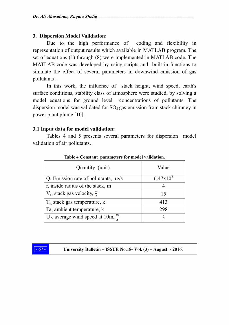
3. Dispersion Model Validation: Due to the high performance of coding and flexibility in

representation of output results which available in MATLAB program. The set of equations (1) through (8) were implemented in MATLAB code. The MATLAB code was developed by using scripts and built in functions to simulate the effect of several parameters in downwind emission of gas pollutants .

In this work, the influence of stack height, wind speed, earth's surface conditions, stability class of atmosphere were studied, by solving a model equations for ground level concentrations of pollutants. The dispersion model was validated for SO2 gas emission from stack chimney in power plant plume [10]. 3.1 Input data for model validation:

Tables 4 and 5 presents several parameters for dispersion model validation of air pollutants.

Table 4 Constant parameters for model validation.

Quantity (unit) Value

Q, Emission rate of pollutants, µg/s 6.47x108 r, inside radius of the stack, m 4 Vs, stack gas velocity, 15

Ts, stack gas temperature, k 413 Ta, ambient temperature, k 298 U2, average wind speed at 10m, 3



Table 5 Simulated parameters for model validation.

Parameter (unit) Value or Class

Wind profile Exponent, p Rough terrain Smooth terrain

0.2 0.12 Stability Class Slightly unstable , C

X, range of downwind distance, km 1,2,4,6,8,10 h=range of stack heights, m 30, 45, 60, 75, 90

3.2 Output results of model validation:

The output results of model validation were displayed graphically to monitor the effect of several parameters in atmospheric air pollutants. The relation between ground level concentration and downwind distance is shown in Figure 1.

1 2 3 4 5 6 7 8 9 100

10

20

30

40

50

60

70

80

90

100

distance down wind (km)

Con

cent

ratio

n at

gro

und

leve

l (m

icro

g/m

3 )

Rough Terrain

Figure 1. Ground level concentrations gas pollutants at several downwind distance.



The ground level concentration is almost zero up to two kilometers of downwind distance, after that the ground level concentration increased rapidly up to six kilometer, then the ground level concentration decreased. The concentration of emitted gas is increased by increasing downwind distance up to 6 km, then the inflection point was noticed .

As can be seen in figure 2, a typical trend curve of wind speed at effective stack heights and ground level concentration was presented. The concentration decreased since this polluted gas was dispersed in atmospheric air and may be transformed to other compounds.

3.2 3.4 3.6 3.8 4 4.2 4.4 4.675

80

85

90

wind speed at effective stack height (m/s)

Con

cent

ratio

n at

gro

und

leve

l (m

icro

g/m

3 )

Rough Terrain

Figure 2. Ground level concentrations of gas pollutants at several stack heights.



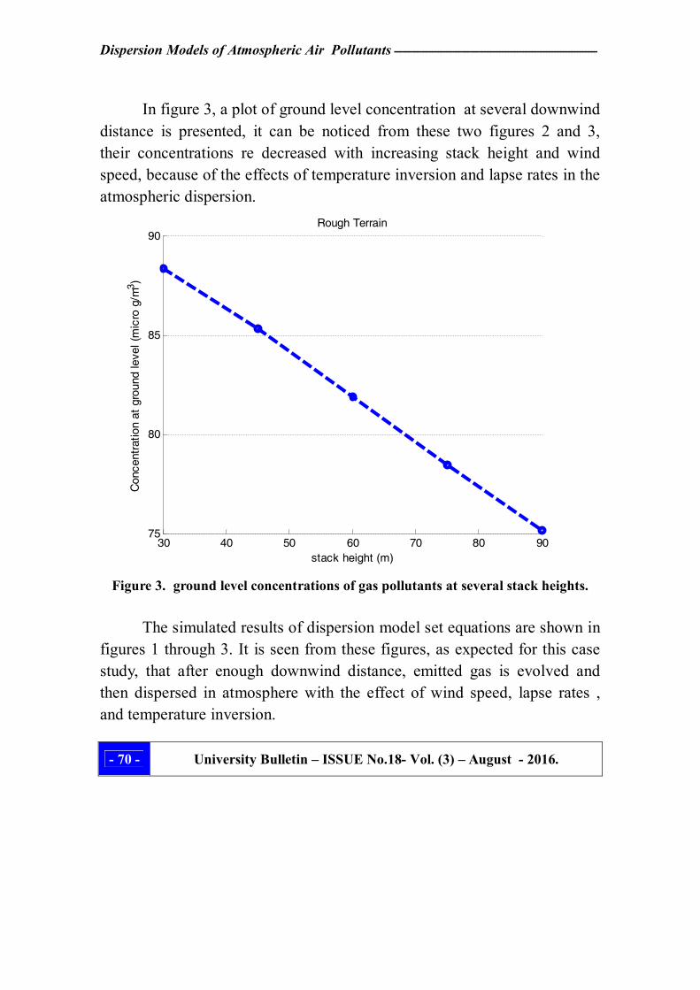
In figure 3, a plot of ground level concentration at several downwind distance is presented, it can be noticed from these two figures 2 and 3, their concentrations re decreased with increasing stack height and wind speed, because of the effects of temperature inversion and lapse rates in the atmospheric dispersion.

30 40 50 60 70 80 9075

80

85

90

Con

cent

ratio

n at

gro

und

leve

l (m

icro

g/m

3 )

stack height (m)

Rough Terrain

Figure 3. ground level concentrations of gas pollutants at several stack heights.

The simulated results of dispersion model set equations are shown in

figures 1 through 3. It is seen from these figures, as expected for this case study, that after enough downwind distance, emitted gas is evolved and then dispersed in atmosphere with the effect of wind speed, lapse rates , and temperature inversion.



In the literature, for air dispersion modeling of emission gases, different models have been proposed [ 4, 5, and 7]. They have concluded that the ground level concentrations of air pollutants was decreased with increasing downwind wind distance and stack height at the same air stability class conditions. 4. Conclusions: Air dispersion models can deal with a number of parameters related to the gas emission and atmospheric dispersion of air pollutants. Air dispersion model of SO2 gas emission from stack chimney in power plant plume have been presented and briefly discussed. The availability of some complex models limits the possibility of utilizing these models in gas emission impact study by some researchers and students. Therefore, due to the high performance of coding and flexibility in representation of output results which available in MATLAB program. The MATLAB code was developed by using scripts and built in functions to simulate the effect of several parameters in downwind emission of gas pollutants . Model validation results suggest that, it is necessary to simulate another case studies of air pollutants with this model to monitor model sensitivity 5. References: 1-Taylor and Francis Group (2006) " Fundamentals of Natural Gas

Processing" Columbus Division, Battelle Memorial Institute and Department of Mechanical Engineering (The Ohio Stat Uni, UAS.

2-Kohl, A.L., and Riesenfeld, f.c. (1985).," Gas purification," 4th Ed .Gulf publishing company, Houston, TX

3-Speight, J.G., (1993), "Gas processing: Environmental Aspects and



Methods."Butterworth Heinemann, oxford, England

4-Newman,S.A. (ed.), (1985), "Acid and Sour Gas Treating processes." Golf Publishing Company, Houston, TX

5-Gollmar, H.A., (1945), Removal of sulphur compounds from coal gas, 947-1007In "chemical of coal Utilization", (H.H .Lowry, (ed). Wiley, New York

6-Gilbert M. Masters, (1991) "Introduction to Environmental Engineering And Science", Prentice-Hall Inc., Englewood Cliffs, New Jersey, USA.

7- Karl B. Schnelle; Charles A. Brown, P.E., (2002), "Air Pollution Control Technology Handbook", New York

8-Robert Macdonald, (2003),"Theory And Objectives Air Dispersion Modeling" , Ph.D thesis,

9–Adel A.Abdel-Rahman, (2008), "On The Atmospheric Dispersion And Gaussian Plume model",

11-Fabrick, A., R.C. Sklarew, and J.D. Wilson , (1977),"point Source Modeling Form& Substance",inc.,Westlake Village, California, USA.

12–Rosmeika, Arief SabdoYuwono, and Dyah Wulandani1, (2014),"Case Study On Air Pollutants Emissions From Boiler Stack Of Biodiesel Plant Using Atmospheric Dispersion Modeling",

13- Aaron Daly and Paolo Zannetti, (2007), "An Introduction to Air Pollution –Definitions, Classifications, and History",

14-Seema Awasthia, Mukesh Khareb and Prashant Gargavac (2006), "General plume dispersion model (GPDM) for point source emission",



6. Apppendix - MATLAB Program:

% %Dispersion model of Atmospheric Air Pollutants

............ %.................Dr. Ali Abusaloua & Eng. Rogia Shelik

%Estimation of Wind Speed at Effective Stack Height by Power Law Correlation z1=[100 125 150 175 200؛[

u2=2.5; z2=10 ؛ %input terrain case؛

% ---- IMPORTANT NOTES ---- %TC=1 means Rough Terrain .. %TC=2 means Smooth Terrain ..

disp(' --input terrain case -- (' disp(' -- TC=1 means Rough Terrain ----(' disp(' -- TC=2 means Smooth Terrain ----('

............................... % TC=input('enter TC as a number 1 or 2('

.............%................... if TC==1

%Rough Terrain disp(' A=1 Unstable;; % B=2 Neutral ;; C:3 Stable('

RC=input('enter RC as 1 | 2| 3(' if RC==1 p=0.15 % ؛

elseif RC==2 p=0.25

else RC==3 p=0.6

end %A= Unstable; p=0.15; % B= Neutral ; p=0.25; C: Stable; p=0.6

for i=1:5 u1(i)=u2*(z1(i)/z2)^p

end ..................................................................... %

else TC==2 %Smooth Terrain

disp(' A=1 Unstable; % B=2 Neutral ; C:3 Stable('؛ RC=input('enter RC as 1 | 2| 3('



if RC==1 p=0.09 % ؛

elseif RC==2 p=0.15

else RC==3 p=0.24

end %A= Unstable; p=0.09; B= Neutral; p=0.15; C: Stable; p=0.24

for i=1:5 u1(i)=u2*(z1(i)/z2)^p

end ..................................................................... %

end %Estimation of Buoyancy Flux Parameter

r=4; Ta=20+273; Ts=100+273; vs=15؛ %Smooth Terrain

F=9.81*r^2*vs*(1-Ta/Ts( ......................... %.......................

% ----------- Estimation of Plume Rise ----------- % --------- For neutral or Unstable Condition ------

if RC==1|2 if F >=55

xf=120*F^0.4 ؛ for i=1:5

dh(i)=1.6*F^(1/3)*xf^(2/3)/u1(i( end else

xf=50*F^(5/8؛( for i=1:5

dh(i)=1.6*F^(1/3)*xf^(2/3)/u1(i( end end

% -------------- %dhRT(i)=1.6*FRT(i)^(1/3)*xf^(2/3؛(

================================================ % .. % .......For stable windy Condition ...........

else RC==3 dTadz=0.02; gamma=0.05؛

S=9.81/Ta*(dTadz+gamma؛( for i=1:5



dh(i)=2.4*(F/u1(i)/S)^(1/3( end end

%dhRT(i)=2.4*(FRT(i)/u1RT(i)/S)^(1/3؛( ======================== %=========================

%input stability Class؛ % ---- IMPORTANT NOTES ---- %SC=A=3 means very unstable ..

%SC=B=4 means moderately unstable .. %SC=C=5 means slightly unstable ..

%SC=D=6 means Neutral .. %SC=E=7 means slightly stable ..

%SC=F=8 means stable .. ............................... %

disp(' --input stability Class -- (' disp(' -- SC=A=3 means very unstable ----('

disp(' -- SC=B=4 means moderately unstable ----(' disp(' -- SC=C=5 means slightly unstable ----('

disp(' -- SC=D=6 means Neutral ----(' disp(' -- SC=E=7 means slightly stable ----('

disp(' -- SC=F=8 means stable ----(' ............................... %

SC=input('enter SC as a number 3 ...8 (' ................................%

%x=input('enter x in km (' %SC=5؛

x=[1 2 4 6 8 10؛[ ............................... %

for j=1:6 if x >= 1 if SC==3

a=213; c=440.8; d=1.941; f=9.27؛ elseif SC==4

a=156; c=106.6; d=1.149; f=3.3؛ elseif SC==5

a=104; c=61; d=0.911; f=0؛ elseif SC==6

a=68; c=33.2; d=0.725; f=-1.7؛ elseif SC==7

a=50.5; c=33.2; d=0.678; f=-1.3؛



else SC==8 a=34; c=14.35; d=0.740; f=-0.35؛

end else x < 1

if SC==3 a=213; c=459.7; d=2.094; f=-9.6؛

elseif SC==4 a=156; c=108.2; d=1.098; f=2.0؛

elseif SC==5 a=104; c=61; d=0.911; f=0؛

elseif SC==6 a=68; c=44.5; d=0.516; f=-13؛

elseif SC==7 a=50.5; c=55.4; d=0.305; f=-34؛

else SC==8 a=34; c=62.6; d=0.18; f=-48.6؛

end end

........................................... % %Estimation of horizontal disp. coeff stad devi, m

sigmay=a*x(j)^0.894 %Estimation of vertical disp. coeff stad devi, m

sigmaz=c*x(j)^d+f ================================================= % Q=6.47e8؛

for i=1:5 H(i)=z1(i)+dh(i( y(i)=z1(i؛(

HE=-H(i)^2/(2*sigmaz^2( YE=-y(i)^2/(2*sigmay^2( cxy(i,j)=(Q/(pi*u1(i)*sigmay*sigmaz))*exp(HE)*exp(YE(

%HRT(i)=z1(i)+dh(i؛( %cxyRT(i)=(Q/(pi*u1(i)*sigmay*sigmaz))*exp(-HRT(i)^2/2*sigmaz^2)*exp(-

y(i)^2/2*sigmay^2( end

end %Estimation of ventilation Coefficient or Atomspheric Dispersive Capabity

dmmax=25; vwavg=0.25; vc0=dmmax*vwavg %vc0=ventilation coeff ؛

%dmmax:maximum mixing depth ؛



%vwavg: ave wind speed .............................،،،،،،،،،،،،،،،،،...............،،،،،،،،،،، %

%Create file for output ! %touch text file.txt

fid=fopen('text.txt', 'w(' for i=1:5

for j=1:6 %fprintf(fid,'% 6.2f \n,i,j(

end end

............................. % if TC==1; % Rough Terrain

figure (1( plot(u1,z1,'linewidth',0.5(

xlabel('wind speed at effective stack height (m/s(' ( ylabel('stack height (m('(

%axis([0.0,15.0,0.0,120.0([ title(' Rough Terrain ('

%legend('C_gas emision', 'Cb','Cc','Cd','Ce','Cf','Cg(' figure (2( subplot(2,1,1( plot(u1,z1,'linewidth',0.5(



%figure (3( subplot(2,1,2( plot(z1,cxy(:,j),'linewidth',0.5(

ylabel(' Concentration at ground level (micro g/m3(' ( xlabel('stack height (m('(


%legend('gas emision', 'Cb','Cc','Cd','Ce','Cf','Cg(' figure (3( subplot(2,1,1( plot(u1,cxy(:,j),'linewidth',0.5(

xlabel('wind speed at effective stack height (m/s(' ( ylabel(' Concentration at ground level (micro g/m3('(

%axis([0.0,15.0,0.0,120.0([



title(' Rough Terrain (' %figure (5(

subplot(2,1,2( plot(x,cxy(i,:),'linewidth',0.5(

xlabel(' distance down wind (km(' ( ylabel(' Concentration at ground level (micro g/m ('(


...... %............................................................... else TC==2; % Smooth Terrain

figure (1( plot(u1,z1,'linewidth',0.5(


%axis([0.0,15.0,0.0,120.0([ title(' Smooth Terrain ('

%legend(' gas emision', 'Cb','Cc','Cd','Ce','Cf','Cg(' figure (2( subplot(2,1,1( plot(u1,z1,'linewidth',0.5(



%figure (3( subplot(2,1,2( plot(z1,cxy(:,j),'linewidth',0.5(

ylabel(' Concentration at ground level (micro g/m3(' ( xlabel('stack height (m('(


%legend('C_gas emisionl', 'Cb','Cc','Cd','Ce','Cf','Cg(' figure (3( subplot(2,1,1( plot(u1,cxy(:,j),'linewidth',0.5(

xlabel('wind speed at effective stack height (m/s(' ( ylabel(' Concentration at ground level (micro g/m3('(




%figure (5( subplot(2,1,2( plot(x,cxy(i,:),'linewidth',0.5(

xlabel(' distance down wind (km(' ( ylabel(' Concentration at ground level (micro g/m ('(


end % .............................

Date post:	03-Feb-2022
Category:	Documents
Upload:	others
View:	27 times
Download:	0 times

Dispersion Models of Atmospheric Air Pollutants

Documents