Page 1
Dispersive Navier-Stokes Systems for
Gas Dynamics: Formal Derivations
C. David Levermore
Department of Mathematics and
Institute for Physical Science and Technology
University of Maryland, College Park
[email protected]
presented 13 August 2013 during the
Summer School and Workshop on
Recent Advances in PDEs and Fluids,
5-18 August 2013, Stanford University, Palo Alto CA
Page 2
Introduction
Many physical systems of partial differential equations from physics that
are dissipative have “corrections” that are dispersive. Examples include:
• so-called α-models of turbulence that have dispersive corrections pro-
portional to a coefficient α,
• so-called dispersive Navier-Stokes systems that have dispersive cor-
rections to classical Navier-Stokes systems of gas dynamics.
The later take two forms: those derived by ad-hoc continuum arguments
and those derived from an underlying kinetic equation. Here we take the
route of kinetic theory, which is a better foundation upon which to build.
Page 3
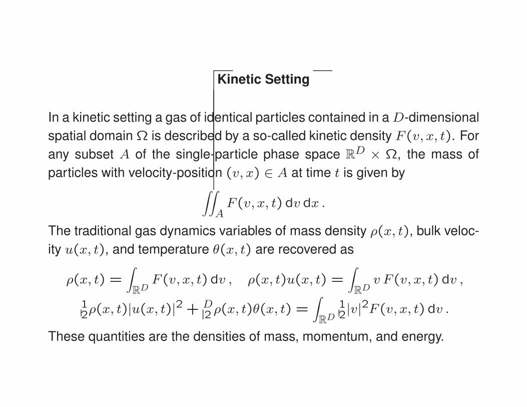
Kinetic Setting
In a kinetic setting a gas of identical particles contained in a D-dimensional
spatial domain Ω is described by a so-called kinetic density F(v, x, t). For
any subset A of the single-particle phase space RD × Ω, the mass of
particles with velocity-position (v, x) ∈ A at time t is given by∫∫
AF(v, x, t) dv dx .
The traditional gas dynamics variables of mass density ρ(x, t), bulk veloc-
ity u(x, t), and temperature θ(x, t) are recovered as
ρ(x, t) =
∫
RDF(v, x, t) dv , ρ(x, t)u(x, t) =
∫
RDv F(v, x, t) dv ,
12ρ(x, t)|u(x, t)|
2 + D2 ρ(x, t)θ(x, t) =
∫
RD
12|v|
2F(v, x, t) dv .
These quantities are the densities of mass, momentum, and energy.
Page 4
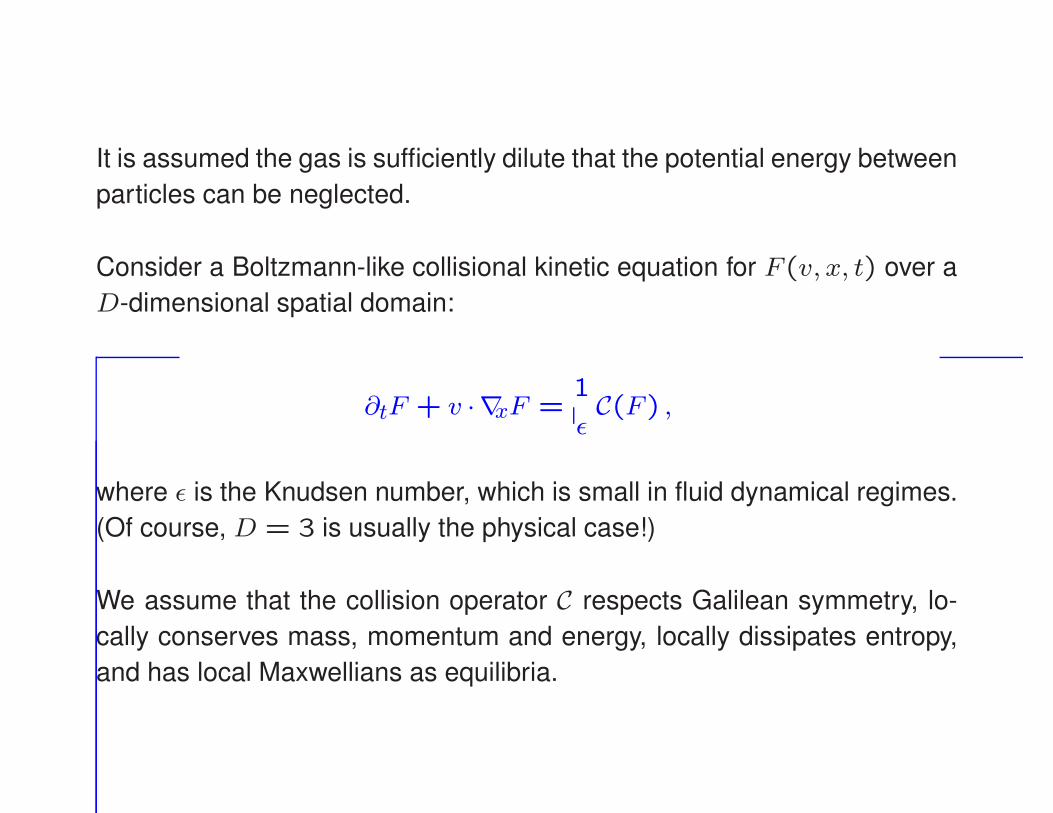
It is assumed the gas is sufficiently dilute that the potential energy between
particles can be neglected.
Consider a Boltzmann-like collisional kinetic equation for F(v, x, t) over a
D-dimensional spatial domain:
∂tF + v ·∇xF =1
ǫC(F) ,
where ǫ is the Knudsen number, which is small in fluid dynamical regimes.
(Of course, D = 3 is usually the physical case!)
We assume that the collision operator C respects Galilean symmetry, lo-
cally conserves mass, momentum and energy, locally dissipates entropy,
and has local Maxwellians as equilibria.
Page 5
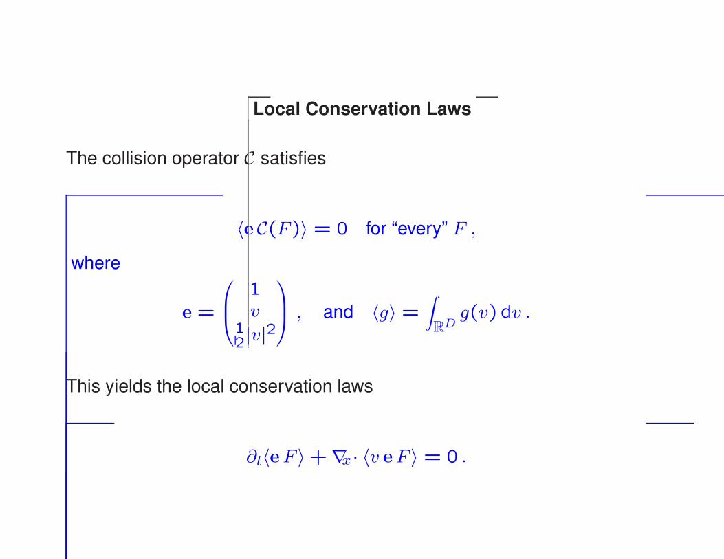
Local Conservation Laws
The collision operator C satisfies
〈e C(F)〉 = 0 for “every” F ,
where
e =
1v
12|v|2
, and 〈g〉 =
∫
RDg(v) dv .
This yields the local conservation laws
∂t〈eF 〉+∇x · 〈v eF 〉 = 0 .
Page 6
Local Entropy Dissipation Law
The collision operator C satisfies
〈η′(F) C(F)〉 ≤ 0 for “every” F ,
where η(F) = F log(F)− F .
This yields the local entropy dissipation law
∂t〈η(F)〉+∇x· 〈v η(F)〉 = 1
ǫ〈η′(F) C(F)〉 ≤ 0 .
Page 7
Local Equilibra
For “every” F the following are equivalent:
(1) 〈η′(F) C(F)〉 = 0 ;
(2) C(F) = 0 ;
(3) F has the Maxwellian form
F = E(ρ) =ρ
(2πθ)D/2exp
(− |v − u|2
2θ
),
where ρ = 〈eF 〉 =
ρρu
12ρ|u|2 + D
2 ρθ
.
Page 8
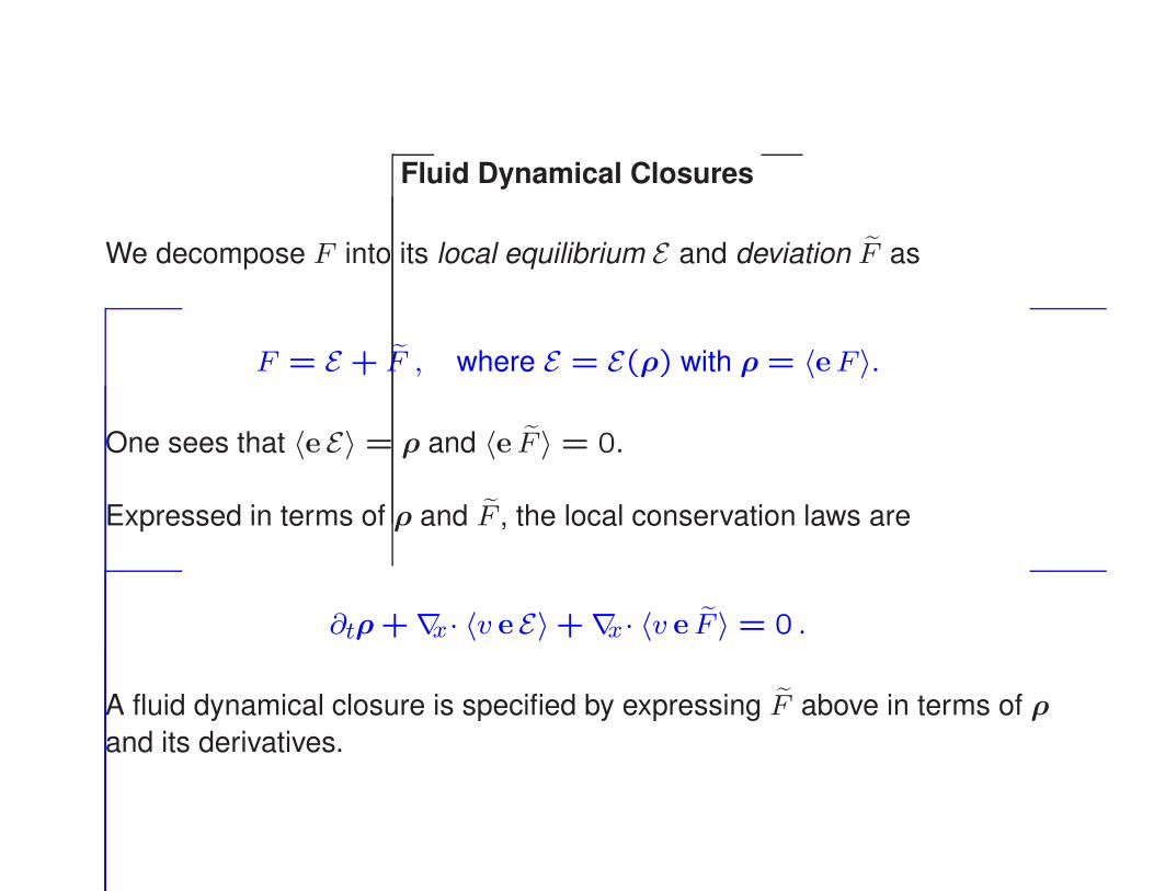
Fluid Dynamical Closures
We decompose F into its local equilibrium E and deviation F as
F = E + F , where E = E(ρ) with ρ = 〈eF 〉.
One sees that 〈e E〉 = ρ and 〈e F 〉 = 0.
Expressed in terms of ρ and F , the local conservation laws are
∂tρ+∇x· 〈v e E〉+∇x · 〈v e F 〉 = 0 .
A fluid dynamical closure is specified by expressing F above in terms of ρ
and its derivatives.
Page 9
Fluid Dynamical System
The resulting fluid dynamical system takes the form
∂tρ+∇x · (ρu) = 0 ,
∂t(ρu) +∇x· (ρu⊗ u+ pI + P ) = 0 ,
∂t(ρe) +∇x · (ρeu+ pu+ P u+ q) = 0 ,
where p = ρθ, e = 12|u|2 + D
2 θ, and
P = 〈A F 〉 , q = 〈B F 〉 ,
with A and B defined by
A = (v − u)⊗ (v − u)− 1D|v − u|2I ,
B = 12|v − u|2(v − u)− D+2
2 θ(v − u) .
Page 10
Euler Approximation
Maxwell first argued that in fluid regimes F should be near its local equi-
librium E . He then observed that F ≈ 0 yields the compressible Euler
system. Its solutions formally dissipate the so-called Euler entropy 〈η(E)〉as
∂t〈η(E)〉+∇x · 〈v η(E)〉 ≤ 0 .
If one wants to improve upon the Euler approximation, one needs a better
approximation for F .
Page 11
Deviation Equation
The deviation F satisfies
∂tF + Pv ·∇xF + Pv ·∇xE =1
ǫC(E + F) ,
where P = I − P with P defined by
P(ρ)f = Eρ(ρ)〈e f〉 .
One can show P and P are orthogonal projections over L2(E−1dv).
Page 12
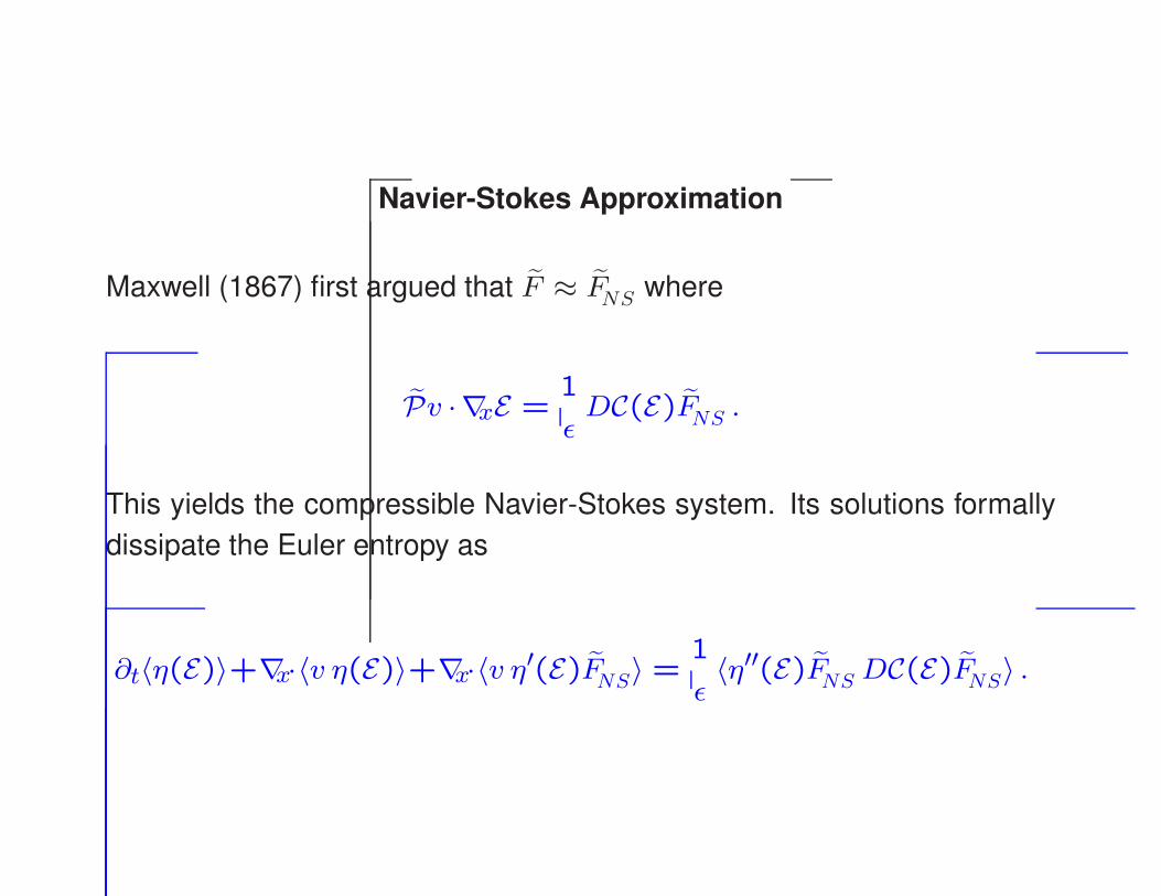
Navier-Stokes Approximation
Maxwell (1867) first argued that F ≈ FNS where
Pv ·∇xE =1
ǫDC(E)FNS .
This yields the compressible Navier-Stokes system. Its solutions formally
dissipate the Euler entropy as
∂t〈η(E)〉+∇x·〈v η(E)〉+∇x·〈v η′(E)FNS〉 =1
ǫ〈η′′(E)FNS DC(E)FNS〉 .
Page 13
Beyond Navier-Stokes Approximations
Hilbert (1912) introduced a derivation of the Navier-Stokes system based
on a systematic expansion in the (small) Knudsen number ǫ. This so-called
Hilbert expansion yields the Euler system at leading order, and corrections
that satisfy linearized Euler systems driven by lower order terms. These
have to be summed through order ǫ to obtain the Navier-Stokes system.
Short afterward, Enskog (1917) introduced a slightly different expansion in
ǫ, subsequently dubbed the Chapman-Enskog expansion, that led directly
to the Navier-Stokes system at order ǫ.
Both these approaches fail to systematically yield corrections to the Navier-
Stokes system that are formally well-posed.
Page 14
An Alternative Approach
We will not use either the Hilbert expansion or the Chapman-Enskog ex-
pansion. Rather, we consider three approximations:
(1) Small Deviation (a kind of linearization)
(2) Material-Frame Stationary Balance (a temporal approximation)
(3) Small Gradient Expansion (a spatial approximation)
All these approximations yield solutions that formally dissipate an entropy,
and are therefore formally well-posed.
Page 15
(1) Small Deviation Approximation
We argue that F ≈ FSD where
AFSD + Pv ·∇xE =1
ǫDC(E)FSD ,
where A = PAP with A defined by
Af =1
2
[(∂t + v · ∇x)f + E (∂t + v ·∇x)
f
E
].
The small deviation system dissipates an entropy as
∂t〈η(E)〉+∇x · 〈v η(E)〉+∇x· 〈v η′(E)FSD〉
+∂t〈12η′′(E)F2
SD〉+∇x · 〈v 1
2η′′(E)F2
SD〉 = 1
ǫ〈η′′(E)FSD DC(E)FSD〉 .
Page 16
Remark: Second Order Entropy Law
If one places F = E + F into the terms of the exact entropy dissipation
law and expand through second order in F one sees that
〈η(E + F)〉 = 〈η(E)〉+ 〈12η′′(E)F2〉+ · · · ,
〈v η(E + F)〉 = 〈v η(E)〉+ 〈v η′(E)F 〉+ 〈v 12η
′′(E)F2〉+ · · · ,〈η′(E + F ) C(E + F )〉 = 〈η′′(E)F DC(E)F 〉+ · · · .
Truncated at second order, the exact entropy dissipation law then becomes
∂t〈η(E)〉+∇x · 〈v η(E)〉+∇x · 〈v η′(E)F 〉
+∂t〈12η′′(E)F2〉+∇x · 〈v 1
2η′′(E)F2〉 = 1
ǫ〈η′′(E)F DC(E)F 〉 .
Page 17
Remark: Relation to Linearization
When E is an exact solution of the kinetic equation then the small deviation
approximation is simply the linearization of that equation about E . Indeed,
one sees that
E is a solution of the kinetic equation ⇐⇒(∂t + v ·∇x
)E = 0
⇐⇒ Af = ∂tf + v · ∇xf .
The small deviation approximation is thereby F ≈ FSD where
∂tFSD + v ·∇xFSD =1
ǫDC(E)FSD .
In this case FSD contains only initial and boundary layers.
Page 18
(2) Material-Frame Stationary Balance Approximation
We argue that F ≈ FMS where
AMSFMS + Pv ·∇xE =1
ǫDC(E)FMS ,
where AMS = PAMSP with AMS defined by
AMSf =1
2
[(v − u) ·∇xf + E ∇x ·
(v − u)f
E
].
The resulting system dissipates the Euler entropy as
∂t〈η(E)〉+∇x· 〈v η(E)〉+∇x · 〈v η′(E)FMS〉
+∇x· 〈(v − u) 12η
′′(E)F2MS
〉 = 1
ǫ〈η′′(E)FMS DC(E)FMS〉 .
Page 19
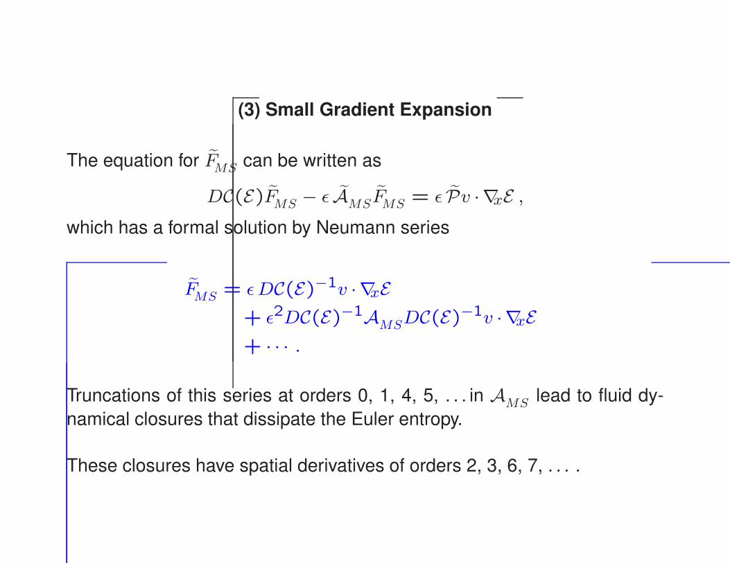
(3) Small Gradient Expansion
The equation for FMS can be written as
DC(E)FMS − ǫ AMSFMS = ǫ Pv ·∇xE ,
which has a formal solution by Neumann series
FMS = ǫDC(E)−1v ·∇xE+ ǫ2DC(E)−1AMSDC(E)−1v ·∇xE+ · · · .
Truncations of this series at orders 0, 1, 4, 5, . . . in AMS lead to fluid dy-
namical closures that dissipate the Euler entropy.
These closures have spatial derivatives of orders 2, 3, 6, 7, . . . .
Page 20
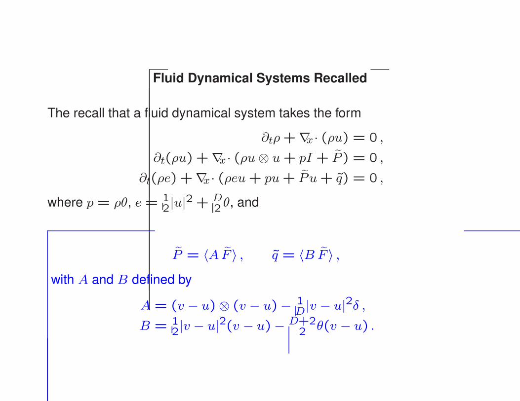
Fluid Dynamical Systems Recalled
The recall that a fluid dynamical system takes the form
∂tρ+∇x · (ρu) = 0 ,
∂t(ρu) +∇x · (ρu⊗ u+ pI + P) = 0 ,
∂t(ρe) +∇x · (ρeu+ pu+ P u+ q) = 0 ,
where p = ρθ, e = 12|u|2 + D
2 θ, and
P = 〈A F 〉 , q = 〈B F 〉 ,
with A and B defined by
A = (v − u)⊗ (v − u)− 1D|v − u|2δ ,
B = 12|v − u|2(v − u)− D+2
2 θ(v − u) .
Page 21
Navier-Stokes Closure - 1
The Navier-Stokes closure takes the form
FNS = −1
θEA :∇xu− 1
θ2EB ·∇xθ ,
where A and B solve
DC(E)EA = EA , DC(E)EB = EB .
By using Galilean symmetry it can be shown that
A = τAA , B = τBB ,
where τA = τA(|v − u|/√θ, ρ, θ) and τB = τB(|v − u|/
√θ, ρ, θ) are
positive and have units of time.
Page 22
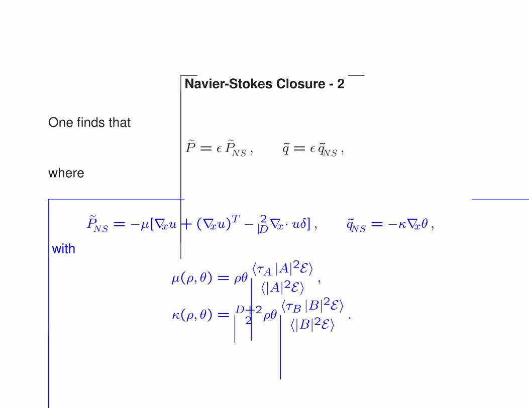
Navier-Stokes Closure - 2
One finds that
P = ǫ PNS , q = ǫ qNS ,
where
PNS = −µ[∇xu+ (∇xu)T − 2D∇x · uδ] , qNS = −κ∇xθ ,
with
µ(ρ, θ) = ρθ〈τA |A|2E〉〈|A|2E〉
,
κ(ρ, θ) = D+22 ρθ
〈τB |B|2E〉〈|B|2E〉 .
Page 23
First Correction to Navier-Stokes - 1
The first correction to the Navier-Stokes system is obtained as
P = ǫ PNS + ǫ2PFC + · · · , q = ǫ qNS + ǫ2qFC + · · · ,
where PNS and qNS are as before, while
PFC = PAAFC
+ PABFC
, qFC = qBAFC
+ qBBFC
,
with
PAAFC
= 12
⟨τ 2A A E(v − u)∇xA
⟩:∇xuθ
− 12
⟨τ 2A A :
∇xuθ
E(v − u) ·∇xA⟩,
Page 24
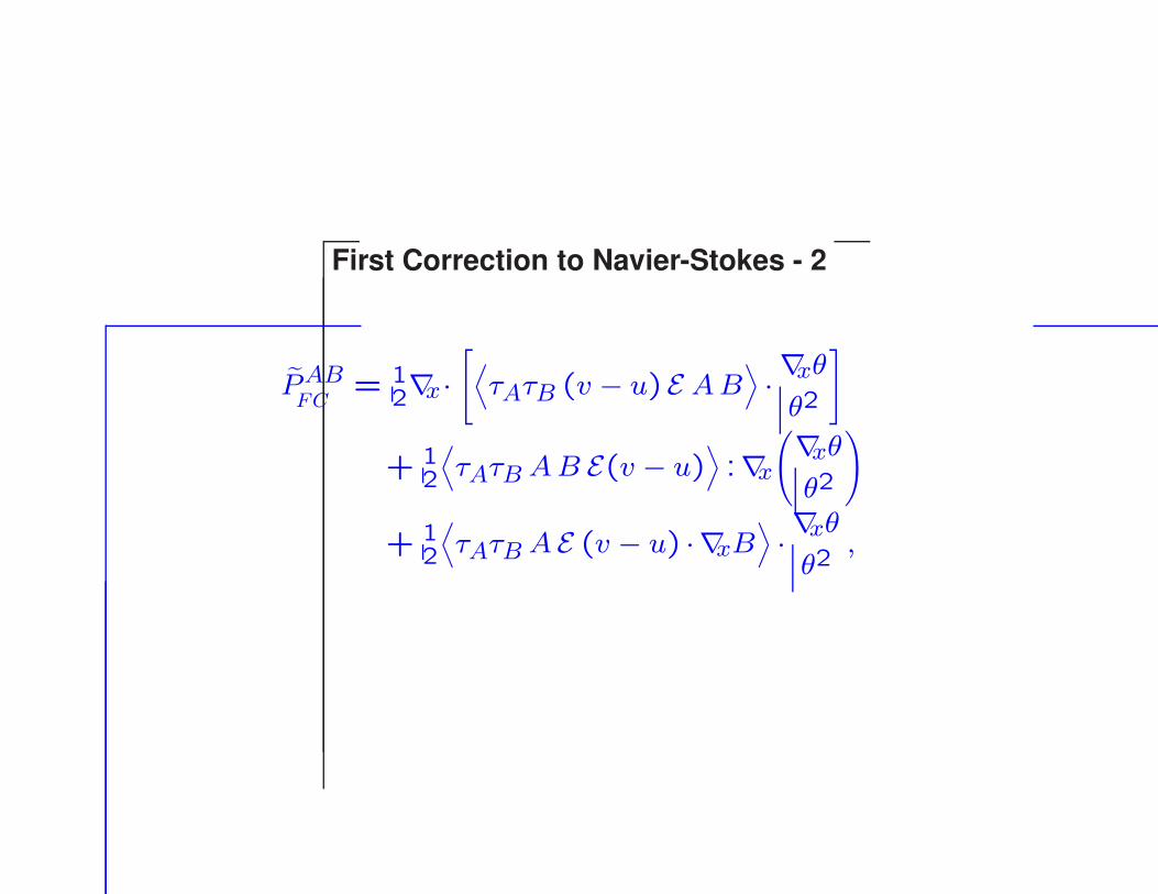
First Correction to Navier-Stokes - 2
PABFC
= 12∇x ·
[⟨τAτB (v − u) E AB
⟩· ∇xθθ2
]
+ 12
⟨τAτB AB E(v − u)
⟩:∇x
(∇xθθ2
)
+ 12
⟨τAτB A E (v − u) ·∇xB
⟩· ∇xθθ2
,
Page 25
First Correction to Navier-Stokes - 3
qBAFC
= 12∇x ·
[⟨τBτA (v − u) E BA
⟩:∇xuθ
]
+ 12
⟨τBτABA E(v − u)
⟩·∇x
(:∇xuθ
)
+ 12
⟨τBτAA ·∇xθ E A
⟩:∇xuθ
,
qBBFC
= 12
⟨τ 2BB E B ·∇xu
⟩· ∇xθθ2
− 12
⟨τ 2BB ·∇xu E B
⟩· ∇xθθ2
.
Page 26
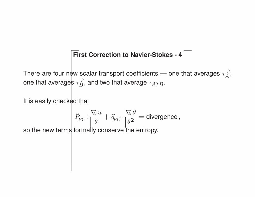
First Correction to Navier-Stokes - 4
There are four new scalar transport coefficients — one that averages τ 2A ,
one that averages τ 2B , and two that average τAτB.
It is easily checked that
PFC :∇xuθ
+ qFC · ∇xθθ2
= divergence ,
so the new terms formally conserve the entropy.
Page 27
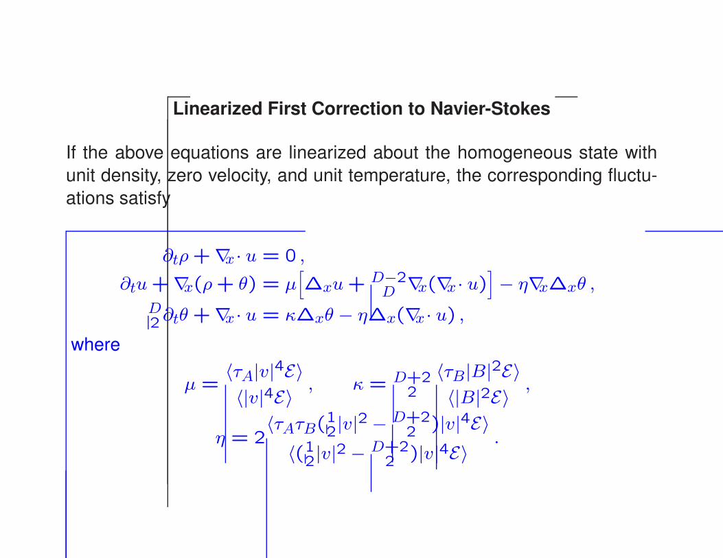
Linearized First Correction to Navier-Stokes
If the above equations are linearized about the homogeneous state with
unit density, zero velocity, and unit temperature, the corresponding fluctu-
ations satisfy
∂tρ+∇x · u = 0 ,
∂tu+∇x(ρ+ θ) = µ[∆xu+ D−2
D ∇x(∇x · u)]− η∇x∆xθ ,
D2 ∂tθ +∇x · u = κ∆xθ − η∆x(∇x · u) ,
where
µ =〈τA|v|4E〉〈|v|4E〉
, κ = D+22
〈τB|B|2E〉〈|B|2E〉
,
η = 2〈τAτB(12|v|2 − D+2
2 )|v|4E〉〈(12|v|2 − D+2
2 )|v|4E〉.
Page 28
Conclusion: Some Open Questions
• What are the correct boundary conditions for these dispersive sys-
tems?
• Are these dispersive systems an improvement? This can be investi-
gated numerically on periodic domains.
• Does one gain more regularity from the additional dispersive terms
than one would expect from the dissipative terms alone? This can be
asked even for the linear system on the previous slide.
• What are good local well-posedness results for classical solutions?