Dissecting Saving Dynamics Measuring Credit, Wealth and Precautionary Effects Christopher Carroll 1 Jiri Slacalek 2 Martin Sommer 3 1 Johns Hopkins University and NBER [email protected]2 European Central Bank [email protected]3 International Monetary Fund [email protected]Presentation at Julis-Rabinowitz Conference Princeton University, February 2014
Transcript
Dissecting Saving DynamicsMeasuring Credit, Wealth and Precautionary Effects
Christopher Carroll1 Jiri Slacalek2 Martin Sommer3
Presentation at Julis-Rabinowitz ConferencePrinceton University, February 2014
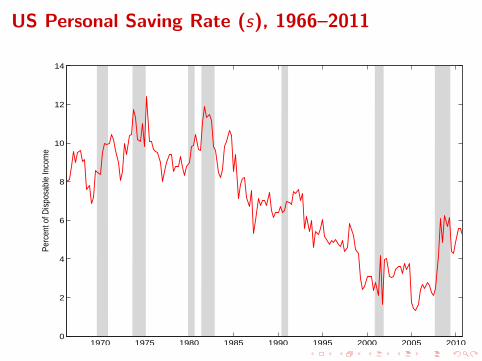
US Personal Saving Rate (s), 1966–2011
1970 1975 1980 1985 1990 1995 2000 2005 20100
2
4
6
8
10
12
14
Perc
ent o
f Dis
posa
ble
Inco
me
Literature
I “Wealth Effects”I Modigliani, Klein, MPS model, ...
I st = −0.05mt + other stuff
I “Precautionary”I Carroll (1992)
I Saving rate rises in recessionsI ∆ logCt+1 strongly related to Et(ut+1 − ut)
I “Credit Availability”I Secular Trend:
I Parker (2000), Dynan and Kohn (2007), Muellbauer (manypapers)
I Cyclical Dynamics:I Guerrieri and Lorenzoni (2011), Eggertsson and Krugman
(2011), Hall (2011)
Great Recession 2007–2009
I s rises by ∼4 pp
I Bigger & more persistent increase than any postwar recessionI But all three indicators also move a lot:
I Credit conditions tightenI Unemployment Expectations riseI Wealth falls
Personal Saving Rate 2007– ↑
−4−2
02
4D
evia
tion
from
Sta
rt−of
−Rec
essi
on V
alue
in %
0 2 4 6 8 10 12 14 16 18 20Quarters after Start of Recession
Historical Range Historical Mean 2007−2011
Our Contributions
I TheoryI Simple model with transparent role for all 3 channelsI Qualitative implications of the model
I “Overshooting” ⇒ possible role for fiscal policy
I EvidenceI Quantify the 3 channelsI Two estimated models of s
I Reduced-form—OLSI Structural—Nonlinear least squares
I ConclusionsI Secular decline in s is almost all from credit ↑I Cyclical movement in s is mostly from w and fI Any big cyclical effect of credit runs through effects on w , f
Theory a la Carroll and Toche (2009)
I CRRA utility, labor supply `, agg wage W, emp status ξ:
v(mmmt) = maxccct
u(ccct) + βEt
[v(mmmt+1)
]s.t.
mmmt+1 = (mmmt − ccct)R + `t+1Wt+1ξt+1
I ξt+1 ∈ {ξu, ξe} where ξu < ξe
I ` and W grow at constant rateI Tractability: unemployment shocks are permanent
I If ξt = ξu then ξt+1 = ξu
I Target wealth m exists and is stable:I Consumption chosen so that mt → m
Target Wealth m
Closed-form solution for target wealth depends on unemploymentrisk f and generosity of unemployment insurance ξu:
m = f ( f(+), ξu
(−), preferences, . . . )
Consumption After a Wealth Shock
Dmt+1e = 0 �
cHmL�
ct � � ct+1
Wealth Shock
� Target
cHmL�
mÇ
mt
m
cÇ
c
Permanent Rise in f
Sustainable c �
� cHmL after unemployment rate increase
� Target
cHmL�
mÇ m
c
Saving Rate After a Permanent Rise in f
� Overshooting
tTime
sÇ
t'
st
Credit Easing/Financial Innovation & Deregulation
� Orig Target� D mt+1
e = 0� Orig cHmL
New cHmL �
-h 0.m
c
m is close to linear in credit conditions
Net Worth (Ratio to Quarterly Disp Income)
44.
55
5.5
66.
5
1970 1975 1980 1985 1990 1995 2000 2005 2010
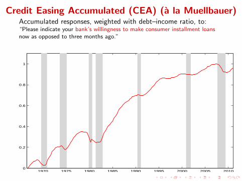
Credit Easing Accumulated (CEA) (a la Muellbauer)Accumulated responses, weighted with debt–income ratio, to:“Please indicate your bank’s willingness to make consumer installment loansnow as opposed to three months ago.”
1970 1975 1980 1985 1990 1995 2000 2005 20100
0.2
0.4
0.6
0.8
1
ft Implied by Michigan U ExpectationsI Regress: ∆4ut+4 = α0 + α1UExptI U risk: ft = ut + ∆4ut+4
I ∆4ut+4 ≡ ut+4 − ut , ∆4ut+4 ≡ fitted valuesI ft tracks but precedes actual U
UExp: “How about people out of work during the coming 12 months—do you think
that there will be more unemployment than now, about the same, or less?”
24
68
10
1970 1975 1980 1985 1990 1995 2000 2005 2010
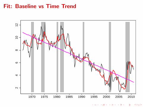
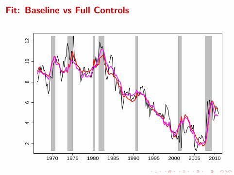
Reduced-Form Regressions
st = γ0 +γmmt +γCEACEAt +γEuEtut+4 +γt t +γuC (Etut+4×CEAt)+εt
Model Time Wealth CEA Un Risk All 3 Baseline Interact
I Easier borrowing largely explains secular decline sI Order of importance in Great Recession:
1. Wealth shock2. Labor income risk3. Credit tightening
I ⇒ if credit has big cyclical effect, comes thru w and f
References
Carroll, Christopher D. (1992): “The Buffer-Stock Theory of Saving: Some Macroeconomic Evidence,”Brookings Papers on Economic Activity, 1992(2), 61–156,http://econ.jhu.edu/people/ccarroll/BufferStockBPEA.pdf.
Carroll, Christopher D., and Patrick Toche (2009): “A Tractable Model of Buffer Stock Saving,” NBERWorking Paper Number 15265, http://econ.jhu.edu/people/ccarroll/papers/ctDiscrete.
Dynan, Karen E., and Donald L. Kohn (2007): “The Rise in US Household Indebtedness: Causes andConsequences,” in The Structure and Resilience of the Financial System, ed. by Christopher Kent, and JeremyLawson, pp. 84–113. Reserve Bank of Australia.
Eggertsson, Gauti B., and Paul Krugman (2011): “Debt, Deleveraging, and the Liquidity Trap: AFisher-Minsky-Koo Approach,” Manuscript, NBER Summer Institute.
Guerrieri, Veronica, and Guido Lorenzoni (2011): “Credit Crises, Precautionary Savings and the LiquidityTrap,” Manuscript, MIT Department of Economics.
Hall, Robert E. (2011): “The Long Slump,” AEA Presidential Address, ASSA Meetings, Denver.
Parker, Jonathan A. (2000): “Spendthrift in America? On Two Decades of Decline in the U.S. Saving Rate,”in NBER Macroeconomics Annual 1999, ed. by Ben S. Bernanke, and Julio J. Rotemberg, vol. 14, pp.317–387. NBER.