Dissecting the Dynamics of the US Trade Balance in an Estimated Equilibrium Model, 2008

FACULTEIT ECONOMIE EN BEDRIJFSKUNDE

TWEEKERKENSTRAAT 2 B-9000 GENT

Tel. : 32 - (0)9 – 264.34.61 Fax. : 32 - (0)9 – 264.35.92

WORKING PAPER

Dissecting the Dynamics of the US Trade Balance in an Estimated Equilibrium Model

Punnoose Jacob

Gert Peersman

November 2008

2008/544

D/2008/7012/53

Dissecting the Dynamics of the US Trade Balance inan Estimated Equilibrium Model�

Punnoose Jacoby Gert Peersmanz

November 26, 2008

Abstract

This paper presents empirical evidence on the stochastic driving forces of the UStrade balance. In an estimated two-country DSGE model, we �nd that investment-speci�c technology shocks have the strongest impact on the volatility of cyclical tradebalance �uctuations, especially when the shocks are domestic and considered overlonger forecast-horizons. At shorter horizons, US and foreign inter-temporal shocksthat generate co-movement between consumption and investment, have an impact com-parable to that of the investment-speci�c technology shocks. In contrast, shocks to USpublic spending and neutral technology - both forces traditionally used to explain tradebalance �uctuations - hardly explain the volatility.

JEL Classi�cation C11, F41

Keywords US Trade Balance, New Open Economy Macroeconomics, Bayesian Infer-ence, DSGE Estimation.

�We acknowledge �nancial support from the Interuniversity Attraction Poles Program-Belgium SciencePolicy (Contract Number P6/07) and the Belgian National Science Foundation (FWO). We thank LievenBaert, Christiane Baumeister, Fabrice Collard, Giancarlo Corsetti, Ferre de Graeve, David de La Croix,Rafael Domenéch, Nicolas Groshenny, Freddy Heylen, Robert Kollmann, Vivien Lewis, Giulio Nicoletti,Morten Ravn, Frank Smets, Raf Wouters, participants at the Dynare Conference 2008 at the Federal ReserveBank of Boston and seminar participants at the National Bank of Belgium for helpful suggestions. Allremaining errors are ours.

yCorresponding Author: Department of Financial Economics, Ghent University, Woodrow Wilsonplein5D, Ghent, Belgium B9000. Email: [email protected]

zDepartment of Financial Economics, Ghent University, Woodrow Wilsonplein 5D, Ghent, BelgiumB9000. Email: [email protected]

1

1 Introduction

The recent experience of the United States on the external sector has spawned a vast liter-

ature in international macroeconomics dwelling on its consequences for the global economy.

The US current account de�cit, both in absolute terms and as a proportion of output, has

reached unprecedented levels in the nation�s �nancial history. This paper disentangles the

stochastic in�uences on the trade balance, the dominant component of the current account.1

Extant macroeconometric work centered on the US trade balance has focussed solely on

the in�uence of domestic shocks. Bems, Dedola and Smets (2007) �nd that �scal shocks

and investment-speci�c technological change have had a negative in�uence on the trade

balance. Corsetti and Konstantinou (2004, 2005) attribute the persistence of the de�cit to

a permanent shock that raises output, consumption and net foreign liabilities. This shock,

interpreted by the authors as a technology shock, dominates the volatility of US net foreign

liabilities over very long horizons. In the short run, transient shocks which decrease net

foreign liabilities play a non-negligible role in explaining the volatility of the variables.

A truism inspires our analysis. Speci�cally, it takes two parties to make a trade balance.

The US trade de�cit absorbs three-fourth of the trade surpluses in the world2 thereby render-

ing any analysis of the US de�cit that ignores in�uences from its trade partners inadequate.

The contribution of this paper is that we explicitly account for disturbances of foreign origin

to in�uence the external position of the US by placing the trade balance in an estimated two

country New Keynesian dynamic stochastic general equilibrium (DSGE) model.

Several authors have examined cyclical �uctuations in the US trade balance in calibrated

two-country DSGE models. The classic contribution of Backus, Kydland and Kehoe (1994)

assesses the link between the terms of trade and the trade balance as well as the responses

of these variables to total factor productivity (TFP) and public spending shocks in an In-

1The US de�cits on the current account and the trade balance equalled (at an annualized rate) 5.74 and5.12 per cent of GDP respectively in 2007. The �gures we use are computed from time series obtained fromthe FRED II database.

2See Obstfeld and Rogo¤ (2005).

2

ternational Real Business Cycle model. Similarly, Kollmann (1998) examines the in�uence

of TFP and �scal shocks. On the other hand, Erceg, Guerrieri and Gust (2005) focus on

the impact of tax and public spending shocks on the external balance in a calibrated New

Keynesian model. Just as the aforementioned authors, we focus on cyclical �uctuations in

the trade balance, while abstracting from the trend.3 However, in contrast to them, we

confront our model with the data in a formal full-information likelihood-based estimation

exercise in order to evaluate the response of the trade balance to a wider array of structural

shocks.

Since we utilize the Bayesian framework to estimate the model, our approach is similar

to other estimated small-scale two-country models in the recent literature like Lubik and

Schorfheide (2005) and Rabanal and Tuesta (2006). Our model though stylized is also much

richer than our precedents as we include capital accumulation and allow imports to enter

the investment basket. The incorporation of the �Rest of the World�(RoW) in an estimated

micro-founded model makes this study the �rst of its type in the empirical literature on the

US trade balance.4

Such a viewpoint, i.e. that of the in�uence of the RoW on the �US�imbalance, has gained

ground in policy-circles in recent times. Ferguson (2005) states that slumps in aggregate

demand and depressed growth in major trade partners such as Japan and the Eurozone

lead to the emergence of the US as a favourable location for investment. Bernanke (2005)

attributes the de�cit to excess saving in the global economy. He suggests that the strong

savings motive of rich countries with aging populations and high capital-labor ratios coupled

3Our methodology only allows detrended data to speak within a stationary environment imposed by alog-linearized DSGE model. The US has been in a trade de�cit since the early 1980s and this paper attemptsto understand the stochastic in�uences that have had positive or negative in�uences on the trade balanceat business cycle frequencies. Other authors, e.g. Engel and Rogers (2006) have examined the long-run pathof the US trade balance.

4Bergin (2006) uses maximum likelihood to estimate a New Keynesian model of the US and the remainingof the G-7 countries. He estimates the model in country di¤erences and hence can only identify relativeshocks. Corsetti, Dedola and Leduc (2005) study the impact of relative productivity shocks on the exchangerate and net exports in impulse response analysis in an SVAR framework. Our DSGE model is asymmetricin the parameters estimated across countries and we intend to identify the structural shocks speci�c to bothregions.

3

with the apparent lack of domestic investment opportunities led them to lend to the US,

hence running external surpluses. Bernanke�s views are echoed by Clarida (2005) who notes

the higher rates of national saving in East Asia and describes the US de�cit as a general

equilibrium phenomenon that is in part caused by a global excess of saving over pro�table

investment opportunities.

Long quarterly series are unavailable for the developing countries whose shares in the

US trade balance have increased in recent times. This undermines the credibility of the use

of the actual time series on the US trade balance in an estimation exercise as ours. We

circumvent this di¢ culty by constructing the aggregated trade balance between the US and

sixteen OECD trade partners with whom the US has experienced de�cits for a reasonably

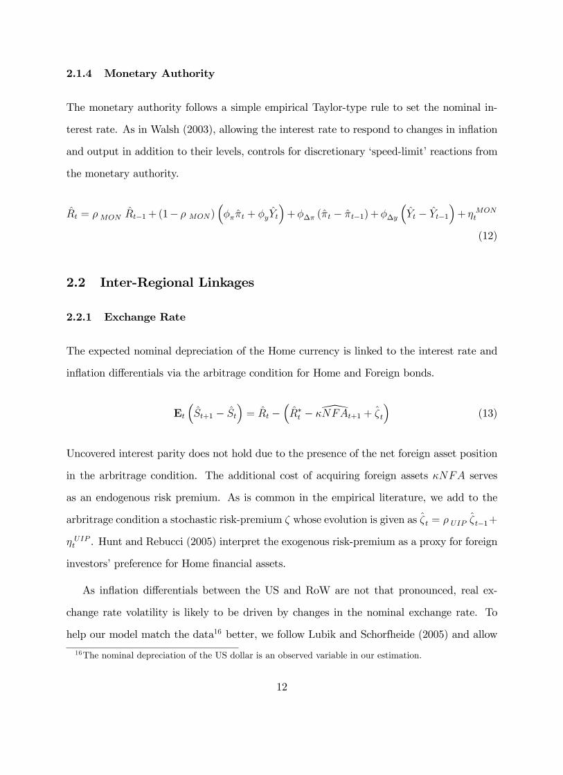
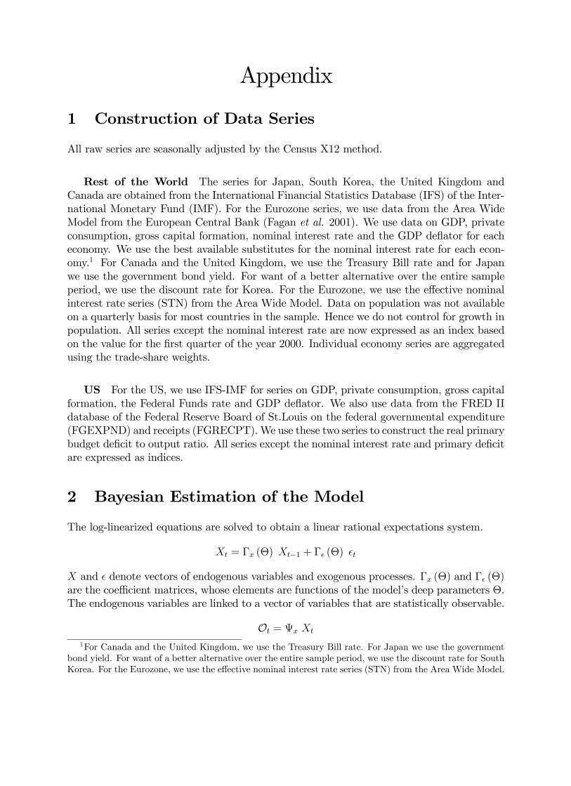
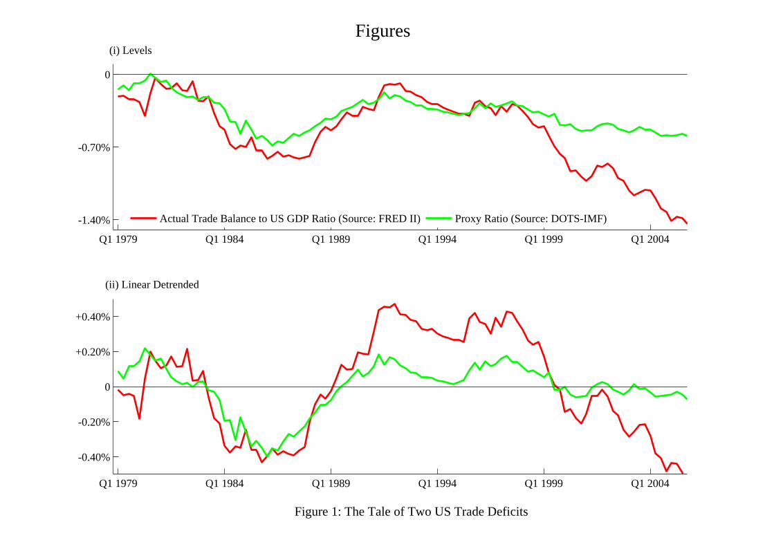
long span of time. As can be seen in Figure 1, the proxy contributes a sizable proportion

of the actual trade de�cit and mimics it remarkably well especially upto the late 1990s. As

we take our two-country model to the data, we utilize trade-weighted time series from the

sixteen OECD economies for the second �country� in the model. As a consequence, this

paper does not take a stand on the actual US trade balance, but restricts attention to the

intra-OECD imbalance.

Insert Figure 1

The estimated model contributes to our understanding of the external position of the

US in a number of ways. The US investment-speci�c technology shock has a very strong

impact on the volatility of cyclical �uctuations in the trade balance to output ratio and is the

predominant in�uence when considered over longer forecast-horizons. At shorter forecast-

horizons, we �nd that inter-temporal disturbances that act as interest rate �wedges� and

a¤ect both the opportunity cost of private consumption as well as the value of physical

capital- and hence raise aggregate demand- have a considerable impact. Both foreign and

US wedge shocks are important and account for about 40 per cent of the volatility in the

short and medium run, decreasing over longer horizons. Further, historical decompositions

4

show that the US investment-speci�c technology shocks and the interest rate wedge shocks

from the Rest of the World contributed strongly and negatively to �uctuations in the trade

balance in the late 1990s.

On the other hand, our results de-emphasize the role of two factors mentioned earlier

in this section as cited in related strands of the literature as explanations of the behaviour

of the US trade balance: those of neutral TFP movements and rises in public expenditure.

For instance, Kollmann (1998) �nds that di¤erentials in TFP between the US and the G-6

economies were the main source of �uctuations in the trade balance over 1975-1991. The

rise in output that follows a domestic TFP shock is dominated by rises in consumption and

investment causing a surge in the demand for imports, resulting in current account de�cits.

We �nd that while the US TFP shock worsens the external position in impulse responses,

it has had a negligible impact on the volatility. Furthermore, others have emphasized the

role of the US Federal government and the consequent �Twin De�cits�on the domestic and

external sectors.5 This paper does not provide an empirical evaluation of the Twin De�cits

hypothesis and reduces the role of public expenditure to a residual in aggregate demand.

However, we �nd that the US public spending shock - just as the US TFP shock- deteriorates

the trade balance in impulse responses but hardly matters for the volatility.

The remainder of the paper is organized as follows. The next section details the theoret-

ical model we set up. Section 3 describes the methodology and construction of the key open

economy data series. Section 4 and 5 present estimation results and our exposition of the

stochastic in�uences that drive �uctuations in the US trade balance over the business cycle.

Section 6 summarizes our main conclusions.5Proponents of the �Twin De�cits�view posit that a lack of public saving deteriorates the nation�s external

position via the national income accounting identity while others have argued that the two de�cits have notbeen twins and have moved even in opposite directions as in the late 1990s. See Erceg et al. (2005), Corsettiand Müller (2006) and the references therein.

5

2 A Two Country Two Sector Model

Our framework has much in common with the work of Smets and Wouters (2007) and Ra-

banal and Tuesta (2006). The model is quite standard in the literature and we do not

present a complete description.6 Our world comprises two regions, each inhabited by in-

�nitely lived consumers, producers and the �scal and monetary authorities. We present

equilibrium conditions for the Home economy that are log-linearized around a simple sym-

metric non-stochastic steady-state with no in�ation, exchange rate depreciation or foreign

asset accumulation. The Foreign region is isomorphic. Foreign region parameters and vari-

ables are denoted by a supercript � and are presented, when essential, in parentheses next

to their Home analogs. Variables that represent a deviation from steady-state are denoted

by b.2.1 Private Agents

2.1.1 Firms

There exists a continuum of intermediate monopolistic �rms each of which produces a unique

variety that can be both consumed and invested. CH (C�F ) and XH (X�F ) are Dixit-Stiglitz

aggregates of individual domestic varieties to be consumed and invested respectively. CF

(C�H) and XF (X�H) are similar aggregates of imported varieties. A distribution sector cost-

lessly produces Armington aggregates of the composite Home and imported bundles for

consumption and investment.

Ct =

�(1� �)

1�C

��1�

Ht + �1�C

��1�

Ft

� ��1

; Xt =

�(1� �)

1�X

��1�

Ht + �1�X

��1�

Ft

� ��1

; � > 0

� denotes the share of imports in the consumption and investment baskets. Note however

that to keep matters simple, we assume that the consumption and investment baskets are

6All our derivations are available on request.

6

equally open to imports. Further, we assume that the Foreign region is as open to Home

region exports. � is the elasticity of substitution between home and foreign goods in both

regions. The price-indices of the domestic and imported bundles are denoted by PH (P �F )

and PF (P �H) respectively.

The �rm rents capital K and labor N from the household at (real) prices rk and w in

perfectly competitive factor markets. Factor payments in the Home country accrue only

to domestic residents.7 It combines the two factors of production using a Cobb-Douglas

technology, so that real marginal cost is a weighted average of factor prices.

\RMCt = (1� �) wt + �rkt � At (1)

where exogenous TFP follows At = � TFP At�1 + �TFPt .

Imperfect Passthrough We follow Benigno (2004) in assuming that the �rm prices

in the currency of the market of destination. This �local-currency pricing�strategy yields

two empirically appealing features in the model. On the one hand, the law of price is

broken at the level of the intermediate varieties and on the other, price stickiness delays

the transmission of exchange rate changes into the aggregate price level in the market of

destination. The �rm, indexed by i, chooses its prices, i.e. �p iHt for domestic sales and �p� iHt

for exports to maximize the value of expected pro�ts.

max�p iHt; �p

� iHt

Et

1X�=0

��t+��t

PtPt+�

�� H��p iHtZHt;� �RMCt+�Pt+�y iHt+�

�+ �� H

�St+l�p

� iHt �RMCt+�Pt+�y iH�t+�

��subject to its demand constraint and indexation rule.

y iHt+� =

�p iHt+�PHt+�

��(CHt+� +Gt+� +XHt+� ) ; y

iH�t+� =

�p� iHt+�P �Ht+�

�� C�Ht+� +X

�Ht+�

�7Similarly, factor payments in the Foreign region accrue only to its residents.

7

ZHt;� =

��1Yl=0

��pHt+l i¤ � > 0 and 1 i¤ � = 0; � > 1; �p 2 (0; 1)

� is the marginal utility of wealth, � is the agent�s subjective discount factor and P denotes

the aggregate price level in the economy. S is the nominal exchange rate, de�ned as the

Home currency price of a unit of foreign currency: a rise in the exchange rate means a

depreciation of the Home currency. The superscript � �indicates that the optimal price set,

cannot be reoptimized in the � periods that follow the decision. As the marginal cost is

independent of output, we can allow the degree of price stickiness to di¤er between domestic

and export sales. However since we do not use data for export prices for the estimation of

the model, we keep the export pricing equations simple by abstracting from indexation.

The Phillips curves for domestic sales are given by

�Ht =�p

1 + ��p�Ht�1 +

�

1 + ��pEt�Ht+1 +

(1� ��H) (1� �H)�H (1 + ��p)

�\RMCt + �dToT t� (2)

��Ft =��p

1 + ��p��Ft�1 +

�

1 + ��pEt�

�Ft+1 +

(1� ��F ) (1� ��F )��F�1 + ��p

� �\RMC

�t + �dToT �t� (3)

dToT and dToT � are the Home and Foreign terms of trade that determine the rate at whichconsumers substitute the imported good for the domestically produced good. They are

de�ned as follows.8 dToT t � PFt � PHt; dToT �t � P �Ht � P �FtThe Phillips curves for export prices are detailed in the section on inter-regional linkages.

8When the law of one price holds dToT �t = �dToT t. Note further that the real exchange rate Q can beexpressed in terms of the nominal exchange rate S and the Home and Foreign terms of trade in the followingway.

Qt =�St + P

�Ft � PHt

��

�dToT t � dToT �t�

8

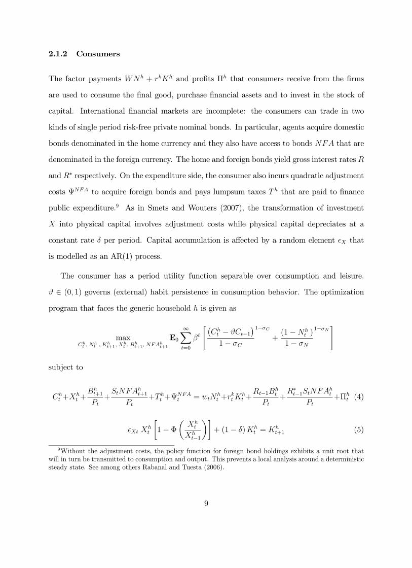
2.1.2 Consumers

The factor payments WNh + rkKh and pro�ts �h that consumers receive from the �rms

are used to consume the �nal good, purchase �nancial assets and to invest in the stock of

capital. International �nancial markets are incomplete: the consumers can trade in two

kinds of single period risk-free private nominal bonds. In particular, agents acquire domestic

bonds denominated in the home currency and they also have access to bonds NFA that are

denominated in the foreign currency. The home and foreign bonds yield gross interest rates R

and R� respectively. On the expenditure side, the consumer also incurs quadratic adjustment

costs NFA to acquire foreign bonds and pays lumpsum taxes T h that are paid to �nance

public expenditure.9 As in Smets and Wouters (2007), the transformation of investment

X into physical capital involves adjustment costs while physical capital depreciates at a

constant rate � per period. Capital accumulation is a¤ected by a random element �X that

is modelled as an AR(1) process.

The consumer has a period utility function separable over consumption and leisure.

# 2 (0; 1) governs (external) habit persistence in consumption behavior. The optimization

program that faces the generic household h is given as

maxCht ; N

ht ; K

ht+1; X

ht ; B

ht+1; NFA

ht+1

E0

1Xt=0

�t

"�Cht � #Ct�1

�1� �C

1��C

+(1�Nh

t )

1� �N

1��N#

subject to

Cht +Xht +Bht+1Pt

+StNFA

ht+1

Pt+T ht +

NFAt = wtN

ht +r

ktK

ht +Rt�1B

ht

Pt+R�t�1StNFA

ht

Pt+�ht (4)

�Xt Xht

�1� �

�Xht

Xht�1

��+ (1� �)Kh

t = Kht+1 (5)

9Without the adjustment costs, the policy function for foreign bond holdings exhibits a unit root thatwill in turn be transmitted to consumption and output. This prevents a local analysis around a deterministicsteady state. See among others Rabanal and Tuesta (2006).

9

NFAt =�

2

StPtYt

�NFAht+1 �NFA

�2; where � > 0; �C ; �N > 0; � 2 (0; 1)

Intra-temporal optimality implies that labor supply is determined by the utility gain from

the real wage.

Nt =1

�Nwt �

�C�N

1

(1� #)Ct +�C�N

#

(1� #)Ct�1 (6)

The inter-temporal �ow of aggregate consumption is decided by the following Euler equa-

tion.10

Ct =1

(1 + #)EtCt+1 +

#

(1 + #)Ct�1 �

1

�C

(1� #)(1 + #)

�Rt � Et�t+1 � "Wt

�(7)

As in Smets and Wouters (2007) "W is a wedge between the interest rate controlled by the

monetary authority and the return on domestic �nancial assets faced by the consumer and

evolves as an AR(1) process. A positive wedge shock decreases the e¤ective rate of return on

assets and stimulates current consumption.11 The wedge also a¤ects the dynamics of Tobin�s

Q and hence investment in physical capital. A positive shock raises the value of capital and

boosts investment. It is this additional e¤ect of the wedge shock that prevents it from being

observationally equivalent to the traditional time impatience shock to the agent�s subjective

discount factor as in Rabanal and Tuesta (2006).

dTQt = (1� � (1� �))Etrkt+1 + � (1� �)EtdTQt+1 � �Rt � Et�t+1 � "Wt

�(8)

The presence of the convex investment adjustment costs implies that investment reacts op-

timally to its own lagged and expected values as well as Tobin�s Q.12

Xt =1

' (1 + �)dTQt + �

(1 + �)EtXt+1 +

1

(1 + �)Xt�1 + ~"Xt (9)

10� is the in�ation rate in the aggregate price level.11Following Smets and Wouters (2007), we rede�ne the interest rate wedge as ~"W � 1

�C

(1�#)(1+#) "W such that

~"Wt = � WED ~"Wt�1 + �WEDt in our estimation.

12The properties of the investment adjustment cost function in the steady state are such that ' = �00 (1) >0;�0 (1) = � (1) = 0

10

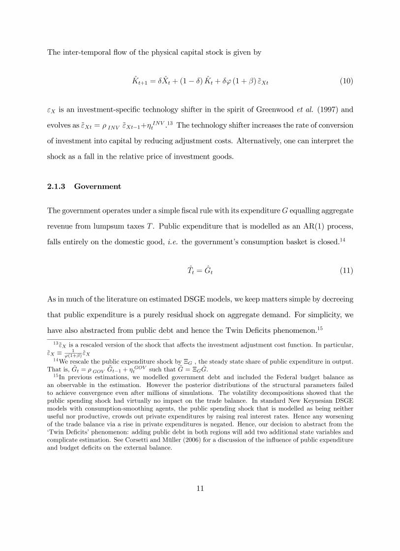
The inter-temporal �ow of the physical capital stock is given by

Kt+1 = �Xt + (1� �) Kt + �' (1 + �) ~"Xt (10)

"X is an investment-speci�c technology shifter in the spirit of Greenwood et al. (1997) and

evolves as ~"Xt = � INV ~"Xt�1+�INVt .13 The technology shifter increases the rate of conversion

of investment into capital by reducing adjustment costs. Alternatively, one can interpret the

shock as a fall in the relative price of investment goods.

2.1.3 Government

The government operates under a simple �scal rule with its expenditureG equalling aggregate

revenue from lumpsum taxes T . Public expenditure that is modelled as an AR(1) process,

falls entirely on the domestic good, i.e. the government�s consumption basket is closed.14

Tt = Gt (11)

As in much of the literature on estimated DSGE models, we keep matters simple by decreeing

that public expenditure is a purely residual shock on aggregate demand. For simplicity, we

have also abstracted from public debt and hence the Twin De�cits phenomenon.15

13~"X is a rescaled version of the shock that a¤ects the investment adjustment cost function. In particular,~"X � 1

'(1+�) "X14We rescale the public expenditure shock by �G , the steady state share of public expenditure in output.

That is, ~Gt = � GOV ~Gt�1 + �GOVt such that ~G = �GG:

15In previous estimations, we modelled government debt and included the Federal budget balance asan observable in the estimation. However the posterior distributions of the structural parameters failedto achieve convergence even after millions of simulations. The volatility decompositions showed that thepublic spending shock had virtually no impact on the trade balance. In standard New Keynesian DSGEmodels with consumption-smoothing agents, the public spending shock that is modelled as being neitheruseful nor productive, crowds out private expenditures by raising real interest rates. Hence any worseningof the trade balance via a rise in private expenditures is negated. Hence, our decision to abstract from the�Twin De�cits�phenomenon: adding public debt in both regions will add two additional state variables andcomplicate estimation. See Corsetti and Müller (2006) for a discussion of the in�uence of public expenditureand budget de�cits on the external balance.

11

2.1.4 Monetary Authority

The monetary authority follows a simple empirical Taylor-type rule to set the nominal in-

terest rate. As in Walsh (2003), allowing the interest rate to respond to changes in in�ation

and output in addition to their levels, controls for discretionary �speed-limit�reactions from

the monetary authority.

Rt = �MON Rt�1+(1� � MON)��t + �yYt

�+�� (�t � �t�1)+��y

�Yt � Yt�1

�+ � MON

t

(12)

2.2 Inter-Regional Linkages

2.2.1 Exchange Rate

The expected nominal depreciation of the Home currency is linked to the interest rate and

in�ation di¤erentials via the arbitrage condition for Home and Foreign bonds.

Et

�St+1 � St

�= Rt �

�R�t � �\NFAt+1 + �t

�(13)

Uncovered interest parity does not hold due to the presence of the net foreign asset position

in the arbritrage condition. The additional cost of acquiring foreign assets �NFA serves

as an endogenous risk premium. As is common in the empirical literature, we add to the

arbritrage condition a stochastic risk-premium � whose evolution is given as �t = � UIP �t�1+

� UIPt . Hunt and Rebucci (2005) interpret the exogenous risk-premium as a proxy for foreign

investors�preference for Home �nancial assets.

As in�ation di¤erentials between the US and RoW are not that pronounced, real ex-

change rate volatility is likely to be driven by changes in the nominal exchange rate. To

help our model match the data16 better, we follow Lubik and Schorfheide (2005) and allow

16The nominal depreciation of the US dollar is an observed variable in our estimation.

12

an idiosyncratic disturbance to a¤ect changes in the exchange rate. This shock captures

deviations from purchasing power parity not accounted for by endogenous frictions such as

local currency pricing and home-bias in trade.

Qt � Qt�1 =�St � St�1

��t � �

�

t

�+ �PPPt (14)

The innovations �xt are independently and identically distributed N (0; �x) and �x 2 (0; 1)

8x:

2.2.2 Export Prices

The Phillips curves for exports sales prices are purely forward looking. The degree of stick-

iness in price adjustment will determine the passthrough of exchange rate changes into the

aggregate price level.17

��Ht = �Et��Ht+1 +

(1� ��H) (1� ��H)��H

n\RMCt � Qt � (1� �)dToT �to (15)

�Ft = �Et�Ft+1 +(1� ��F ) (1� �F )

�F

n\RMC

�t + Qt � (1� �)dToT to (16)

2.2.3 Goods Market Clearing

Domestic output in each region is absorbed by �xed proportions of consumption and invest-

ment at home and abroad as well as exogenous domestic government spending.

Yt = �C

�(1� �)Ct + �C�t

�+�X

�(1� �)Xt + �X

�t

�+��(1��) (�C + �X)

�dToT t � dToT �t�+ ~Gt(17)

Y �t = �C

�(1� �)C�t + �Ct

�+�X

�(1� �)X�

t + �Xt

�+��(1��) (�C + �X)

�dToT �t � dToT t�+ ~G�t(18)

17Note that the aggregate in�ation is a convex combination of in�ation in domestic sales prices and importprice in�ation, i.e. �t = (1� �)�Ht + ��Ft

13

�C and �X are the steady-state shares of consumption and investment in output.

2.2.4 Balance of Payments

The balance of payments between the two regions is determined by the inter-temporal �ow

of net foreign assets (as a proportion of output).

\NFAt+1 �1

�\NFAt = ��C

�C�t � Ct

�+ ��X

�X�t � Xt

�+ � (�C + �X) Qt

+� (1� �) (�C + �X) (�� 1)�dToT t � dToT �t� (19)

The trade balance (net exports) to output ratio of the Home economy, expressed in terms

of the consumption and investment baskets, the terms of trade and the real exchange rate is

given by the right hand side of the above equation.18 Note how adjustments in savings and

investment via the trade balance are facilitated by a concurrent movement in the net foreign

asset position, i.e. the capital account.

3 The Case for a Proxied Trade Balance

The acquisition of dollar-denominated assets by economies as China, the oil-producing

economies and to a lesser extent Brazil, Russia and India have received the recent attention of

pundits, policy-makers and the media alike in the context of the US de�cit. However, quar-

terly data series spanning reasonably long time-spans are unavailable for these economies.

This undermines the credibility of using the actual time series on the US trade balance, i.e.

vis-á-vis all countries including the emerging markets, in an estimation exercise as ours.

Given the sometimes con�icting objectives of considering a long enough sample period

while also maintaining consistency over the selection of countries that run surpluses with

18If one removes investment from the model, i.e. set �X = 0 ; the structural equations reduce to those ofthe model featuring incomplete-markets with local currency pricing posited in Rabanal and Tuesta (2006).

14

the US, we restrict ourselves to the OECD and choose economies that have mostly been

net lenders to the US. In particular, we choose Canada, Japan, South Korea, the United

Kingdom and twelve economies in the Eurozone to form our aggregate of the RoW. We then

construct the aggregated bilateral trade balance of the US vis-á-vis the sixteen economies,

thereby circumventing the di¢ culty of controlling for the economies omitted from our sample.

A weighted aggregate of these sixteen OECD economies now constitutes our measure of the

RoW and the �proxy�trade balance that channels savings and investment �ows between the

US and the aggregate of economies is the centerpiece of our empirical analysis.

Interestingly, despite not including in our RoW aggregate the high-saving economies of

Asia that have drawn the speci�c attention of policy makers, the long-run imbalance between

savings and investment prevails even in our synthetic two-country world. Figure 2 depicts

crude measures of savings ratios and investment ratios in our aggregate of economies and

the US over 1980-2005. It is clear that while the RoW has always met its investment needs

with su¢ cient rates of savings, the opposite has been the case with the US. The savings

and investments ratios in both regions were roughly in balance in the early 1980s, diverged

as the years progressed and returned to approximate balance by the end of the decade. In

1991-92, the US savings-investment gap was close to zero. Strikingly, at this very point in

time, the RoW also bridged its savings-investment gap. From this point of balance, the

ensuing decade and a half saw drastic changes. The high savings-lower investment gap in

the RoW became quite persistent towards the late 1990s. The US experience was exactly

the opposite, with private saving- having trended downward throughout the sample period-

turning very low by the turn of the millenium.

Insert Figure 2

Equipped with the intuition about the long-run di¤erentials in savings-investment be-

havior in the two regions, we attempt a business cycle analysis of the �uctuations of the US

15

trade balance around its trend as we estimate our two country model and analyze the im-

pact of the various shocks on the trade balance. Without doubt, leaving out the non-OECD

economies handicaps our analysis and imperils inference. Note further that our two-country

framework also restricts us to view all the economies that constitute the RoW as a uni�ed

economic region, thereby abstracting from all heterogeneity in economic behavior across the

sixteen economies. The structural parameters for the RoW including those pertaining to

the monetary policy rule have to be seen as a weighted average. However, despite the many

limitations of our RoW aggregate and the stylized two-country approach, we demonstrate

in our estimation of the theoretical model how our arti�cial equilibrium environment can be

used as a laboratory to understand the forces that in�uence the actual disequilibrium.

3.1 Construction of Key Open Economy Series

We use the Direction of Trade Statistics (DOTS) database of the IMF to construct the

aggregated bilateral trade balance (net exports in US dollars). Panel (i) of Figure 1 compares

the sample aggregated trade balance to output ratio as a proportion of US GDP with the

actual series over the time period we consider. Omitting many of the non-OECD economies

in our aggregate implies that there is some disparity in size between the two series. However,

until the late 1990s the proxy tracks the actual series rather well. The two series have high

correlation coe¢ cients of 0.85 in levels and 0.77 after linear detrending. The gap between

the two series increases by the turn of the millenium, understandably due to the emergence

of the Asian economies as major trade partners of the US.

Unlike other studies that use multi-country aggregates, we avoid using real GDP weights

to aggregate the series for the individual economies which constitute the RoW.19 We use

trade-share weights instead that may better emphasize the role of each country in the inter-

regional transmission of shocks. Shares of each individual economy are computed by dividing

19See Bussiëre et al. (2005) and Bergin (2006) among others.

16

the sum of imports and exports with the individual economy by aggregate trade. They are

exhibited in Panel (i) of Figure 3. We use the trade-share weights to aggregate individual

nominal exchange rates of the dollar vis-á-vis the trade parters.20 We display a comparison

of the depreciation of the constructed exchange rate and the Nominal E¤ective Exchange

Rate of the IMF in Panel (ii) of Figure 3. The correlation is high between the actual series

and the constructed series at 0.81. The trade shares are then used to aggregate the time

series obtained for the individual economies. All particulars are detailed in the Appendix.

Insert Figure 3

3.2 Bridging the Theory and the Data

We use 12 quarterly series over the period 1980.I to 2005.IV to identify the structural para-

meters in the model. In addition to the trade balance and the nominal exchange rate, we use

series on real GDP, real consumption, real investment, nominal interest rate and the GDP

de�ator for both the US and the RoW. We multiply the natural logarithms of consumption,

output, investment, the price level and the nominal exchange rate by 100. These series are

fed into the model in demeaned �rst di¤erences. The demeaned nominal interest rates are

divided by 4 to translate them into quarterly terms. The nominal interest rates and the

linearly detrended trade balance to US GDP ratio enter the estimation in levels.

4 Estimation Methodology

We follow the Bayesian estimation methodology of Smets and Wouters (2007). A brief

description is presented in the Appendix.

20Individual country nominal exchange rates were obtained from the IMF-IFS database. The pre-EMUEuro-Dollar exchange rate was constructed using the methodology of Lubik and Schorfheide (2005) harnessingcountry-weights from the Area Wide Model.

17

4.1 Prior Distributions

Estimated Parameters An overview of all priors that we set are presented in Table 1.

As we have virtually no information on structural parameters in the constructed aggregate of

economies, we use the priors identical to those used for the US. As in Lubik and Schorfheide

(2005), we set Gamma priors of mean 2 and standard deviation 0.5 for the risk-aversion coef-

�cients (�C ; �C�). The external habit parameters (#; #�) are given Beta priors of mean 0.50

and standard deviation 0.15. Similar to Smets and Wouters (2007), we use a loose Normal

prior of mean 4 and unit variance for the investment adjustment cost parameters ('; '�).

We set Normal priors of mean 2 and unit variance for the duration of pricing contracts

(�; ��) which is interpretable as a price change every three quarters.21 For the indexation

parameters,��p; �

�p

�we set Beta priors on mean 0.50 and standard deviation 0.15. We use

loose priors on the monetary policy rule: the in�ation coe¢ cients (��; ��) are given Normal

priors of mean 1.5 and unit variance. All other coe¢ cients��y; �y�; ��y; ��y�; ��; ��

�are given Gamma priors of mean 0.50 and standard deviation 0.25. The interest rate smooth-

ing parameters in the policy rules are given Beta priors of mean 0.50 and standard deviation

0.15.

The intratemporal elasticity of substitution between Home and Foreign goods, a subject

of much discussion and debate in international macroeconomics, is given a loose Uniform

prior between 0.001 and 7. Estimates of this parameter obtained in similar structural models

are in the vicinity of unity.22 All shock persistence parameters are given Beta priors of mean

0.50 and standard deviation 0.15. We use Inverse Gamma priors with mean 0.10 and standard

deviation 2 for the standard deviations of the shocks.

Calibrated Parameters As we do not use data on wages or hours worked, we calibrate

the frisch elasticities of labor�

1�N; 1�N�

�. As in Smets and Wouters (2007), they are �xed

21As in Rabanal and Tuesta (2006), we de�ne � = 11��H � 1 so that the average duration of pricing

contracts exceeds one quarter.22See Bergin (2006) and Rabanal and Tuesta (2006).

18

at 0.5. Similarly, due to non-availability of data for exports and imports prices vis-á-vis

the economies in our sample, we �x the degree of price-stickiness in the export sales sector.

We set the mean duration of price changes in export sales at two quarters. The subjective

discount factor (�), the share of capital in the production function (�) and the quarterly

depreciation rate of capital (�) are set at 0.99, 1/3 and 0.025 respectively. This implies a

steady-state share of investment in output (�X) of about 0.24. The steady-state consumption

to output ratio (�C) is set to 0.60. The cost of acquiring foreign assets (�) is given a value

of 0.001. We impose considerable home bias in consumption and investment expenditures

by setting the openness parameter (�) at 0.15. This value is in the range obtained in the

literature : Backus et al. (1994) set the parameter at 0.15, Rabanal and Tuesta (2006) obtain

posterior estimates varying between 0.05 and 0.16 while Bergin (2006 ) uses a value of 0.20.

4.2 Posterior Distributions and Impulse Responses

We report the results of the posterior optimization and monte carlo simulation in Table 1 and

the marginal posterior distributions are displayed in Figure 4. We comment on the median

values of the marginal distributions of selected parameters. The elasticity of substitution

between home and foreign goods, a critical parameter in open economy models, is found to

be in the range obtained in other studies. The posterior median is seen to be at 0.9, slightly

lower than estimates found by Rabanal and Tuesta (2006) and Bergin (2006) but higher

than the estimates of Lubik and Schorfheide (2005). The distribution of this parameter is

fairly tightly spread around the traditional benchmark of unity used in the open economy

literature: despite the loose and �at prior, the posterior spans from about 0.8 to 1.1.

Insert Table 1

Parameters governing inter-temporal substitution in consumption appear to be quite

dissimilar between the two regions. For the risk aversion coe¢ cients, we �nd a value of

19

about 1.7 for the US and 2.6 for the RoW. The habit coe¢ cient for the US is found to be

low at 0.2. The RoW analog is even lower at about 0.1. The estimates of the investment

adjustment cost parameter in the US is slightly lower than Smets and Wouters (2007) at

about 4.75. The RoW analog is almost identical. The estimates for the average length of

pricing contracts is between 2 and 3 quarters for both the US and the RoW. The US price

indexation parameter is very similar to that of Smets and Wouters (2007) at about 0.26.

The RoW analog is lower at about 0.14. All shocks show high persistence, with the AR(1)

coe¢ cients of both TFP shocks nearly hitting the boundary of unity. However, notably the

UIP risk premium shock is relatively less persistent than in other studies, at about 0.84.

Bergin (2006) �nds a point estimate of 0.97 while Rabanal and Tuesta (2006) �nd posterior

means ranging between 0.91 and 0.94 in various speci�cations.

Insert Figure 4

We present the impulse responses to some key variables in Figure 5. The 5th and 95th

percentiles and the median of the posterior distribution are displayed for each of the twelve

shocks in the model. To save on space, we present only the responses of the main components

of the trade balance: relative consumption�C � C�

�, relative investment

�X � X�

�, and the

real exchange rate�Q�. The responses of the country-speci�c variables behave in a standard

way and are similar to other closed economy estimations such as Smets and Wouters (2007)

and are not displayed in the �gure.23 In our discussion, we focus on the impact of US shocks

on the trade balance, the exchange rate and the domestic US variables as the responses

induced by the RoW analogs are similar.

Insert Figure 5

23Impulse responses for other variables are available upon request.

20

Investment-speci�c Technology Shocks In the short run the investment-speci�c

technology shock, that increases the e¢ ciency of conversion of the good into the capital

stock, resembles a demand-type shock. Investment spending rises in the US, leading to a

persistent rise in output. The monetary authority raises the interest rate to stabilize output

and in�ation, which has a negative impact on US consumption. However in the medium and

long run, the shock acts more like a supply-type shock when wealth e¤ects raise consumption.

The rise in relative investment is the single most important factor in explaining the short-

and medium term decline in the trade balance in this case. The immediate impact on the

dollar is a strong real appreciation, before it starts to rise after about eight quarters. The

depreciation of the currency leads to an improvement in the trade balance in the long run

before it returns to steady-state.

Interest Rate Wedge Shocks The inter-temporal shock appears as a wedge between

the policy interest rate and the rate that faces the economic agent. On impact, consumption

and investment spending rise in the US, inducing positive responses from output, in�ation

and the nominal interest rate. Notably relative investment rises more sharply and persistently

than relative consumption. This demand-type shock causes a real appreciation of the US

dollar and the terms of trade. The result is a strong deterioration in the US external position.

Note that a negative wedge shock, that increases savings and lowers investment in the RoW

mimics the US shock as far as the responses from the external variables are concerned.

TFP Shocks Despite the extreme persistence of the US TFP shock, its quantitative

impact on the trade balance is mild in comparison to the investment-speci�c technology

shock and the interest rate wedge shock. A rise in US TFP invokes positive responses

from consumption and investment as the permanent income of the agents rise. It decreases

US in�ation and the interest rate leading to a strong real depreciation of the dollar and

a concurrent deterioration of the US terms of trade. On impact, the strong expenditure

21

switching e¤ect of the dollar depreciation improves the trade balance by increasing exports,

but in the medium-term the negative impact of rising relative consumption and investment

dominates the expenditure switching e¤ect and the trade balance deteriorates.

Public Spending Shocks In response to a US public spending shock, the US nominal

interest rate rises strongly due to the central bank response to the rise in in�ation following

the surge in aggregate demand. This crowds out US consumption and investment while

appreciating the US dollar. The appreciated dollar also raises in�ation and the interest rate

in the RoW decreasing consumption and investment. In e¤ect, relative consumption shows

a decline while the impact on the relative investment is insigni�cant. These two e¤ects are

dominated by the real appreciation of the dollar that causes US exports to fall due to a

strong negative expenditure switching e¤ect, causing the trade balance to decline. While

the quantitative impact of public spending shocks on the trade balance is stronger than the

response induced by neutral productivity, it is still considerably milder than the impact of

the interest-rate wedge shocks and investment-speci�c technological shocks.

Risk Premium Shock to the Exchange Rate A rise in the risk premium on foreign

borrowing depreciates the US dollar, raises the US interest rate and lowers the RoW interest

rate. This reduces US consumption and investment while increases the RoW analogs.The im-

pact of the falling relative consumption and investment are reinforced by positive movements

in the exchange rate and the terms of trade. In e¤ect, the US external position improves.

Monetary Policy Shocks Contractionary monetary policy leads to a decrease in US

investment, consumption, output and in�ation. The dollar appreciates via the interest parity

condition making imports cheaper and improving the US terms of trade. Similar to the case

of the public spending shock, the trade balance deteriorates as the impact of the dollar

appreciation dominates the fall in relative consumption and investment.

22

Purchasing Power Parity Shock The impact of the purchasing power parity shock

that disturbs the deterministic relationship between the nominal and the real exchange rates

is statistically insigni�cant for all variables except for the US dollar that experiences a strong

nominal appreciation. The shock, the most di¢ cult to interpret among all the stochastic

in�uences in the model, seems to be the driving force of the nominal exchange rate. Just

as in Lubik and Schorfheide (2005), the dynamics of the exchange rate exhibit considerable

disconnect from the fundamentals formally modelled.24

5 Determinants of Fluctuations in the Trade Balance

5.1 Volatility Decomposition

The in�uence of the twelve shocks that we embedded in the theoretical construct are re-

�ected in the conditional variances of the forecast errors given by the estimated model. We

dissect the volatility of the forecast error of the trade balance to output ratio to reveal the

contributions of the shocks on an individual basis. Note that we do not implement the

decomposition at a particular point in the parameter space, e.g. at the posterior mode or

median. Instead, we use 250 random draws from the posterior to generate a distribution

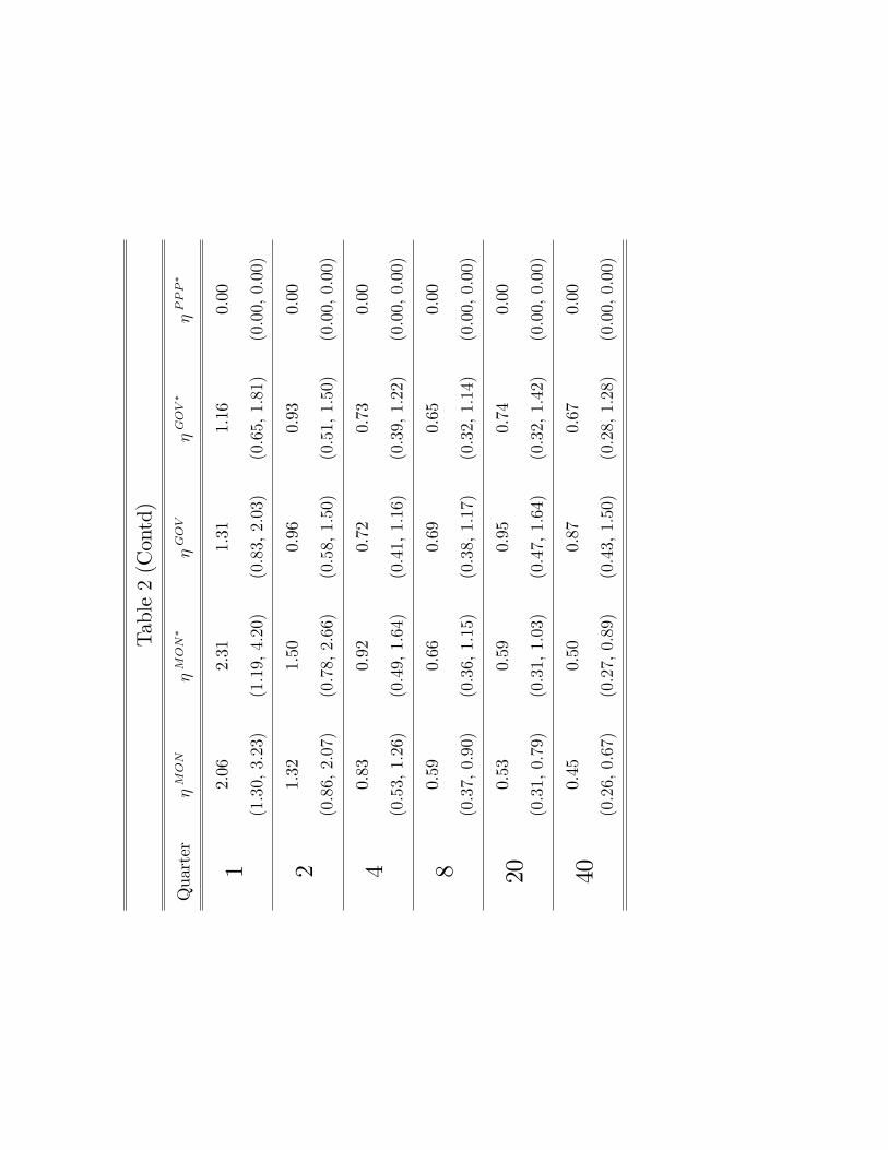
of forecast error volatility decompositions. We report the 5th and 95th percentiles and the

median value of the contributions of the individual shocks to the trade balance to output

ratio in Table 2.25

Both US and RoW monetary policy shocks appear to have little impact on the trade

balance. Public spending shocks also play a negligible role: the median contribution of the

24The PPP disturbance accounts for almost 80% of the conditional forecast volatility of the nominaldepreciation of the US dollar. The variance decomposition of the nominal depreciation of the US dollar isavailable on request.25Our strategy of relying on random draws of parameters instead of a particular point in the parameter

space implies that the median percentage contributions of the shocks do not add up to 100. The decompo-sition at the mode, that is invariant to the results of posterior simulation, is very similar and is presented inTable 3.

23

US shock barely comes to 2 per cent at all horizons. In our world of forward-looking agents

that smooth consumption inter-temporally, exogenous increases in (unproductive) public

spending crowds out private consumption due to the rise in real interest rates. Thus any

worsening of the external position by a stimulation of private expenditures is precluded.

However, simulation results in Erceg et al. (2005) con�rm the negligible in�uence of public

spending shocks on the external position, even in models with non-ricardian features as

liquidity-constrained consumers who cannot smooth their consumption inter-temporally and

hence are insensitive to changes in the interest rate.26

Unlike Bergin (2006), who �nds that the risk premium shock to the exchange rate, de-

termines about two-thirds of the variation in the external balance (current account), we �nd

that this shock plays a muted role. The median contribution comes to about 17 per cent on

impact and its role decreases over time to a minimal 8 per cent over the very long run. The

lower contribution of the risk premium shock is possibly due to our lower estimate of the

persistence parameter.

5.1.1 Neutral versus Investment-Speci�c Technology Shocks

Neutral technology shocks to TFP, with the US shock being the most persistent of all shocks

in the model, do not cause much variability in the trade balance. The combined median e¤ect

of the TFP shocks at home and abroad never exceeds 2 per cent. The weak in�uence of TFP

on the trade balance is in contrast to Kollmann (1998) who �nds that TFP di¤erentials

betwen the US and the G-6 economies were the main source of �uctuations in the trade

balance over 1975-1991. In contrast, our results suggest that the rise in consumption and

investment that TFP induces are insu¢ cient to generate much variability in the external

position, as the strong depreciation of the currency o¤sets these negative e¤ects. We �nd

26In an empirical test of the two competing traditional explanations of the US external position, i.e.neutral productivity vis-á-vis the �scal balance, Bussiëre et al. (2005) �nd a statistically signi�cant e¤ectof TFP on the US trade balance while the �scal position appears to matter very little. Both Bussiere et al.(2005) and Erceg et al. (2005) allow for rule-of-thumb consumers who are liquidity constrained, in order toallow for a rise in private consumption following a public spending shock.

24

that the technological shocks speci�c to investment, however have a very strong impact.

The contribution of the US investment-speci�c shock increases over time and contributes

in excess of 40 per cent the long horizon of 10 years. At all horizons, this shock strongly

dominates its RoW analog whose contribution remains stable over time at about 10 per cent.

In the long run, the combined e¤ect of these investment shocks dominate that of all other

shocks.

The strong in�uence of the investment-speci�c shock vis-á-vis the neutral TFP shock,

is mainly due to the di¤erent responses the two shocks evoke from the real exchange rate.

In the short run following impact of the investment-speci�c shock, the sharp rise in private

investment crowds out private US consumption due to the hike in the real interest rate. The

consequent dollar appreciation induces expenditure-switching e¤ect in favor of imports from

the RoW. In the long run, even though the dollar depreciates and stimulates US exports,

consumption rises due to the wealth-e¤ect that a technology shock typically induces. The

combined negative impact of rising consumption and investment in the long run, dominates

the positive impact of the depreciating dollar. This is in contrast to the neutral TFP shock

that depreciates the dollar so strongly that the consequent expenditure switching in favor

of US exports smothers the negative impact of rising consumption and investment.27 The

considerable impact of investment-speci�c technological shocks on the trade balance is con-

sistent with the structural VAR results in Bems et al. (2007) who only check the impact of

US shocks.

Upto the �rst year following impact, the trade balance is mainly driven by the interest

rate wedge shocks that generate comovement between consumption and investment. In

unison, the median contributions of the shocks range between 30 and 40 per cent at all

horizons. As in the case of investment-speci�c shocks, the US wedge shock dominates the

RoW analog. While the role of the US shock remains stable over time at about 22 per cent,

27For a comparison between the two types of technological shocks in a closed-economy context, see Jus-tiniano et al. (2008).

25

the contribution of the RoW shock decreases slightly from 15 per cent to 10 per cent.

Evidence of the considerable in�uence of the wedge shocks from outside the US that

have negative impacts on RoW consumption and investment supports the arguments of

policymakers that factors boosting saving in the RoW have considerable impact on the US

position. The strong contributions of these interest-rate wedges to the volatility of the trade

balance in the short and medium run, suggest that the determination of the US external

position stretches beyond purely technological di¤erences between the US and the Rest of

the World.

Insert Table 2

5.1.2 Beyond Technology: Net Worth Shocks?

Recent theoretical papers by Mendonza, Quadrini and Rios-Rull (2007) and Caballero, Farhi,

and Gourinchas (2008) relate the US current account position to progress in the sophisti-

cation of �nancial intermediation in the US vis-á-vis the rest of the world. The key point

that these authors raise is that in a world of well integrated but heterogenous �nancial mar-

kets, the more �nancially developed economy experiences a decline in the external balance

by attracting savings from the other. In our model, a positive interest rate wedge shock in

conjunction with the real interest rate acts as a lowering of the e¤ective opportunity cost

of current expenditure, boosting aggregate demand by a¤ecting the inter-temporal marginal

conditions in much the same way as for e.g. highly liquid capital markets or rising asset

prices would. These e¤ects are similar to the �net-worth�mechanism posited in Bernanke,

Gertler and Gilchrist (1999). A wealth-transfer as a net-worth shock that increases the

agent�s wealth typically raises the value of capital by driving up the demand for physical

capital for investment purposes and hence output as well. In our case, these wealth e¤ects

appear strong enough to a¤ect the external balance.

If this shock was speci�ed in the model as a¤ecting private consumption alone as in the

26

earlier generation of estimated DSGE models, it would capture merely a time impatience

e¤ect to the economy�s discount factor. However, the fact that the wedge shock a¤ects the

value of capital as well and the empirical observation that investment appears to react much

more robustly than consumption to the realization of the shock, makes it a likely candidate for

a ��nancial�disturbance rather than a pure preference shock. A sophisticated formulation of

a �nancial intermediation sector or asset prices, their role in boosting aggregate demand and

the consequent impact on a nation�s external position is beyond the scope of our empirical

two country model. However, the predominant role of the inter-temporal �opportunity cost�

wedges in driving �uctuations in the US trade balance makes a compelling case for the

validity of this channel. In the long run, the combined e¤ect of these shocks reduces and the

the investment-speci�c technology shocks dominate.

5.2 The Experience of the 1990s through the Lens of the Model

An oft-repeated theme in the literature is the real appreciation of the dollar and the simul-

taneous plummeting of the trade balance in the later years of the 1990s. Hunt and Rebucci

(2005) state that labor productivity in the tradable goods sector played a major role in these

events. They �nd that augmenting a version of the IMF-GEM model with a TFP shock,

a risk premium shock proxying foreign investor�s preferences for US assets and learning in

expectations formation can help it to match the data satisfactorily. The productivity view

has also been examined by Corsetti, Dedola and Leduc (2007) in VAR estimations. The

thesis is that the rise in labour productivity appreciated the dollar and the terms of trade

via classic Harrod-Balassa-Samuelson e¤ects and concurrently eroded the trade balance.

We contribute to the above literature by examining the explanatory power of each shock

in the estimated model to the evolution of the proxy trade balance in the 1990s. The 1990s

are of interest in our empirics for a number of reasons. The proxy trade balance matches the

actual series in this time-span and the correlation between the two increases to 0.92 in levels.

27

Furthermore, from the long-run savings-investment di¤erential depicted in Figure 2, we can

see that it was during the early 1990s, that savings and investment in our two country world,

were last noted to be in approximate balance in both regions: the origin of contemporary

global �nancial imbalances can be traced to the beginning of that decade.

Note from Panel (ii) of Figure 1 that for both the proxy and the actual trade balance,

�uctuations from their respective trends were positive in this decade.28 We now attempt to

understand the factors that contributed negatively and positively to the US external position

in the 1990s by implementing a historical decomposition of the proxy trade balance using the

best estimates of the structural parameters and the residuals.29 To examine the contribution

of each of the twelve shocks in the model to the evolution of �uctuations in the proxy trade

balance in the 1990s, we start from a benchmark of zero for the �rst observation in our

sample and then simulate the model forward. The contribution of a shock to the trade

balance must be understood as how the trade balance would have evolved in a world where

the only in�uence on the trade balance was the shock itself. The results are presented in

Figure 6.

Not surprisingly, the main actors in our volatility decomposition exercise, namely the

investment-speci�c shocks, the UIP risk premium shock and the interest rate wedge shocks,

also play dominant roles in the historical evolution of the series. This is even as shocks

to TFP, public spending and monetary policy have barely any explanatory power. In our

discussion below, we focus on the shocks that had a substantial impact.

Insert Figure 6

We observe distinct patterns in the in�uence of various shocks for the early 1990s and the

later years of the decade. In the �rst half of the decade, US investment-speci�c technology28We remind the reader that a positive deviation from the trend should not be interpreted as a US trade

surplus. In our exercise, we study which shocks help track the evolution of the detrended series.29We implement the historical decomposition at parameter values set at the mode of the posterior distri-

bution.

28

shocks made a positive contribution to the observed series as did the RoW interest rate

wedge shocks. The positive impact of these shocks appear to have been smothered by the

strong negative contribution of UIP risk-premium shocks and US interest rate wedge shocks.

The net e¤ect on the trade balance, however, was positive. The roles of the shocks reversed

towards the end of the decade. The mid- and the late 1990s saw the in�uence of UIP shocks

and US interest rate wedge shocks turn positive. The downward pressure seems to have been

exerted by an extremely strong negative impact of US investment-speci�c shocks and RoW

interest rate wedge shocks.

The strong negative in�uences of US investment-speci�c technology shocks and (negative)

RoW interest rate wedge shocks towards the late 1990s are intuitive. This was a period when

the US entered an era of prosperity heralded by the arrival of the �New Economy�. The surge

in investment - and the rise in consumption that gradually follows in the aftermath of an

investment speci�c shock- had a negative impact on the trade balance. Concurrently, the

in�uence of the RoW interest rate wedge shock, that dislocated savings from the Rest of the

World to the US had a similar negative impact.on the US position. The 1990s were �nancially

turbulent times for two major US trade partners in our sample. Monetary uncertainty

prevailed in Western Europe in the period preceding the institution of the Euro and Japan

was already experiencing vapid economic growth throughout the 1990s. We conjecture that

these external factors could have made the RoW a less favourable location for investment

and contributed to the relocation of savings into the US, that was experiencing prosperous

times during the same period. However the net e¤ect of these shocks was positive as far as

�uctuations in the trade balance from the trend are concerned.

6 Conclusion

The primary contribution of this paper is the examination of the US trade balance in an em-

pirical two country DSGE model. We investigate the degree to which a variety of stochastic

29

in�uences, both of US and foreign origin, matter for �uctuations in the US trade balance.

US investment-speci�c technology shocks have a very strong and persistent in�uence on the

trade balance and dominate the impact of all other shocks embedded in the model in the

long run. In the short and medium run, we �nd that inter-temporal disturbances that cre-

ate wedges between the interest rate set by the monetary authority and the one that faces

the economic agent, have a strong in�uence. The considerable in�uence of (negative) inter-

temporal disturbances from the RoW in the volatility decomposition indicates that factors

that boost saving and lower investment abroad appear to have a negative impact on the ex-

ternal position of the US. Since these shocks have similar dynamic e¤ects as the �net-worth�

mechanism posited in the literature, we conjecture that- in addition to technological changes

- relative advancement in �nancial intermediation has had a strong negative impact on the

external position of the US over the sample period.

We also �nd that two factors previously cited in the literature as important determinants

of the US external position, namely public spending shocks and TFP, have had relatively

little in�uence on the trade balance, as compared to the shocks to consumption and invest-

ment. While the US public spending shock can worsen the external position by inducing

a strong appreciation of the currency, its impact on the volatility of the trade balance is

negligible. Similarly, shocks to TFP, despite exhibiting extreme persistence, have had very

little in�uence on the volatility. Domestic technology shocks if neutral as in the case of TFP

movements, tend to depreciate the currency strongly and the consequent expenditure switch-

ing e¤ect in favour of US exports compensates the negative impact of rising US consumption

and investment.

Note however that a few caveats are in order. The results regarding the negligible in�u-

ence of the US public spending shock should be taken with a grain of salt. Given the historical

observation that the �Twin De�cits�prevailed in the mid-1980s and the post-millennial years

while moving in opposite directions in the late 1990s, it is likely that the e¤ect of changes in

the �scal position on the external balance has changed over time. We cannot observe these

30

e¤ects in our theoretical model as the role of public expenditure in the determination of

aggregate demand is restricted to being merely residual. It may be instructive to consider a

more elaborate role of public spending in the economy by allowing it to either a¤ect private

utility or the production function. Further, our approach, both in the construction of the

theoretical model and in its statistical implementation, is insu¢ cient to study the persistent

downward trend in the US trade balance over the sample period. A negatively trending

trade-balance would be a useful facility in a structural model of the US trade balance and

in our analysis using detrended data, we are constrained in examining sustainability of the

external position or exploring the consequences of an unwinding of the imbalance. These

avenues, undoubtedly challenging, could be explored in future empirical research.

The above caveats notwithstanding, we are optimistic that empirical insights that have

emerged from the use of our proxy trade balance in the model environment are useful to

visualize the actual imbalance as a global phenomenon instead of one that is necessarily

�made-in-the-USA�, in the absence of concurrent in�uences from the Rest of the World.

Afterall it takes two parties to make a trade balance.

References

[1] Backus, David, Patrick Kehoe and Finn Kydland,1994. "Dynamics of the Trade Balanceand the Terms of Trade: The J-Curve?". American Economic Review 84, pp.84-103.

[2] Bauwens, Luc, Michel Lubrano and Jean-Francois Richard, 1999. "Bayesian Inferencein Dynamic Econometric Models". Oxford University Press.

[3] Benigno, Gianluca, 2004. �Real Exchange Rate Persistence and Monetary Policy Rules,�Journal of Monetary Economics 51, pp.473-502.

[4] Bergin, Paul, 2006. "How Well can the New Open Economy Macroeconomics Explainthe Exchange Rate and Current Account?". Journal of International Money and Finance25, pp.675-701.

[5] Bernanke, Ben, 2005. "The Global Savings Glut and the US Current Account".Remarks at the Sandridge Lecture, Virginia Association of Economics, Richmond.http://www.federalreserve.gov/boarddocs/speeches/2005/20050414/default.htm

31

[6] Bernanke, Ben, Mark Gertler and Simon Gilchrist, 1999. "The Financial Acceleratorin a Quantitative Business Cycle Framework". In J. B. Taylor & M. Woodford (ed.),Handbook of Macroeconomics, Edition 1, Vol. 1, pp.1341-1393.

[7] Bussiérre, Matthieu , Marcel Fratzcher and Gernot Müller, 2005. "Productivity Shocks,Budget De�cits and the Current Account". European Central Bank Working Paper No.509.

[8] Caballero, Ricardo, Emmanuel Farhi, and Pierre-Olivier Gourinchas, 2008. "An Equi-librium Model of "Global Imbalances" and Low Interest Rates". American EconomicReview 98, pp.358-393.

[9] Calvo, Guillermo, 1983. "Staggered Prices in a Utility Maximizing Framework". Journalof Monetary Economics 12, pp.383-398.

[10] Clarida, Richard, 2005. "Japan, China and the US Current Account De�cit". CatoJournal 25, pp.111-114.

[11] Corsetti, Giancarlo, Luca Dedola and Sylvain Leduc, 2006. "Productivity, ExternalBalance and Exchange Rates: Evidence on the Transmission Mechanism Among G7Countries". NBER Working Paper No. 12483.

[12] Corsetti, Giancarlo and Panagiotis Konstantinou, 2005. "Current Account Theory andthe Dynamics of the US Net Foreign Liability Position". CEPR Discussion Paper No.4920.

[13] Corsetti, Giancarlo and Panagiotis Konstantinou, 2004. "Macroeconomic Dynamics andthe Accumulation of Net Foreign Liabilities in the US: An Empirical Model". In "Dollars,Debt and De�cits: 60 Years After Bretton Woods." IMF.

[14] Corsetti, Giancarlo and Gernot Müller, 2006. "Twin De�cits: Squaring Theory, Evi-dence and Common Sense". Economic Policy 48, pp.597-638.

[15] Engel, Charles and John Rogers, 2006. "The U.S. Current Account De�cit and theExpected Share of World Output". Journal of Monetary Economics 53, pp.1063-1093.

[16] Erceg, Christopher, Luca Guerrieri and Christopher Gust, 2005. "Expansionary FiscalShocks and the US Trade De�cit". International Finance 8, pp.363-397.

[17] Fagan, Gabriel, Jérôme Henry and Ricardo Mestre, 2001. "An Area-Wide Model (AWM)for the Euro Area". European Central Bank Working Paper No. 42.

[18] Ferguson, Roger, 2005. "US Current Account De�cits: Causes and Consequences". Re-marks in a speech at the Economics Club at the University of North Carolina at ChapelHill. http://www.federalreserve.gov/boarddocs/Speeches/2005/20050420/default.htm

[19] Greenwood, Jeremy, Zvi Hercowitz and Per Krusell, 1997. "Long-run Implications ofInvestment-speci�c Technological Change". American Economic Review 87, pp.342-362.

32

[20] Justiniano, Alejandro, Giorgio Primiceri and Andrea Tambalotti, 2008. �InvestmentShocks and Business Cycles�. Northwestern University Mimeo.

[21] Kollmann, Robert, 1998. "US Trade Balance Dynamics: The Role of Fiscal Policy andProductivity Shocks and of Financial Market Linkages". Journal of International Moneyand Finance 17, pp.637-669.

[22] Lubik, Thomas and Frank Schorfheide, 2005. "A Bayesian Look at the New OpenEconomy Macroeconomics". NBER Macroeconomics Annual 20, pp.313�366.

[23] Mendoza, Enrique, Vincenzo Quadrini and José-Victor Rios-Rull, 2007. "FinancialIntegration, Financial Development and Global Imbalances". NBER Working PaperNo.12909.

[24] Obstfeld, Maurice and Kenneth Rogo¤, 2005. "Global Current Account Imbalances andExchange Rate Adjustments". Brookings Papers on Economic Activity 36, pp.67-146.

[25] Rabanal, Pau and Vincente Tuesta, 2006. "Euro-Dollar Real Exchange Rate Dynamicsin an Estimated Two-Country Model: What is Important And What is Not". CEPRDiscussion Paper 5957.

[26] Smets, Frank and Rafael Wouters, 2007. "Shocks and Frictions in US Business Cycles:A Bayesian DSGE Approach". American Economic Review 97, pp.586-606.

[27] Walsh, Carl, 2003. "Speed Limit Policies: The Output Gap and Optimal MonetaryPolicy". American Economic Review 93, pp.265-278.

33

Appendix

1 Construction of Data Series

All raw series are seasonally adjusted by the Census X12 method.

Rest of the World The series for Japan, South Korea, the United Kingdom andCanada are obtained from the International Financial Statistics Database (IFS) of the Inter-national Monetary Fund (IMF). For the Eurozone series, we use data from the Area WideModel from the European Central Bank (Fagan et al. 2001). We use data on GDP, privateconsumption, gross capital formation, nominal interest rate and the GDP de�ator for eacheconomy. We use the best available substitutes for the nominal interest rate for each econ-omy.1 For Canada and the United Kingdom, we use the Treasury Bill rate and for Japanwe use the government bond yield. For want of a better alternative over the entire sampleperiod, we use the discount rate for Korea. For the Eurozone, we use the e¤ective nominalinterest rate series (STN) from the Area Wide Model. Data on population was not availableon a quarterly basis for most countries in the sample. Hence we do not control for growth inpopulation. All series except the nominal interest rate are now expressed as an index basedon the value for the �rst quarter of the year 2000. Individual economy series are aggregatedusing the trade-share weights.

US For the US, we use IFS-IMF for series on GDP, private consumption, gross capitalformation, the Federal Funds rate and GDP de�ator. We also use data from the FRED IIdatabase of the Federal Reserve Board of St.Louis on the federal governmental expenditure(FGEXPND) and receipts (FGRECPT).We use these two series to construct the real primarybudget de�cit to output ratio. All series except the nominal interest rate and primary de�citare expressed as indices.

2 Bayesian Estimation of the Model

The log-linearized equations are solved to obtain a linear rational expectations system.

Xt = �x (�) Xt�1 + �� (�) �t

X and � denote vectors of endogenous variables and exogenous processes. �x (�) and �� (�)are the coe¢ cient matrices, whose elements are functions of the model�s deep parameters �.The endogenous variables are linked to a vector of variables that are statistically observable.

Ot = x Xt

1For Canada and the United Kingdom, we use the Treasury Bill rate. For Japan we use the governmentbond yield. For want of a better alternative over the entire sample period, we use the discount rate for SouthKorea. For the Eurozone, we use the e¤ective nominal interest rate series (STN) from the Area Wide Model.

Invoking Bayes theorem, we know that if p () indicates the prior information available on thevector of structural parameters � and L (O j �) is the conditional likelihood function of thedata, the posterior density is given by

P (� j O) / p (�) L (O j �)

The estimation is implemented in the following steps.

1. The Kalman �lter is used to evaluate the logarithm of the posterior density

2. The Sims optimizer is used to �nd the mode ~� of the posterior density. The inverseof the Hessian ~�� is evaluated at the mode.

3. The posterior density is simulated using the Random Walk Metropolis Algorithm thatis initiated at the mode of the posterior. For n = 1..nsim, draw � (n) from a multivariatenormal jumping distribution N

�� (n�1); c2 ~� �1

�

�. � (n) is accepted with a probability

min�1; �

�� (n);� (n�1) j O

��or rejected

�� (n) = � (n�1)� otherwise.

�� (n);� (n�1) j O

�=

p�� (n)

�L�O j � (n)

�p (� (n�1)) L (O j � (n�1))

c2 is adjusted to obtain an acceptance rate of about 34 %. We use 1 long chain ofnsim = 1,000,000.

4. The initial 10,000 draws are discarded. The expected values of h (�) are approximatedusing the draws

h (�) =

nsimXn=10;001

h�� (n)

�Chain convergence is monitored using CUSUM statistics as in Bauwens et al. (1999).Impulse responses and the decomposition of the volatility of the trade balance arecomputed using 250 random draws from the posterior density.

Q1 1979 Q1 1984 Q1 1989 Q1 1994 Q1 1999 Q1 2004

-1.40%

-0.70%

0

(i) Levels

Q1 1979 Q1 1984 Q1 1989 Q1 1994 Q1 1999 Q1 2004

-0.40%

-0.20%

0

+0.20%

+0.40%

(ii) Linear Detrended

Actual Trade Balance to US GDP Ratio (Source: FRED II) Proxy Ratio (Source: DOTS-IMF)

Figure 1: The Tale of Two US Trade Deficits

Figures

Q1 1980 Q1 1982 Q1 1984 Q1 1986 Q1 1988 Q1 1990 Q1 1992 Q1 1994 Q1 1996 Q1 1998 Q1 2000 Q1 2002 Q1 2004Q4 2005

-05%

0

+05%

+10%

+15%

+20%

+25%

+30%

+35%

RoW Gross Savings

RoW Gross Investment

US Gross Savings

US Gross Investment

US Private Savings

Gross Savings Ratio = (Y-C-G )/ (Y-G)Gross Investment Ratio = X/ (Y-G)Private Savings Ratio = (Y-C-T)/ (Y-G)

Figure 2: The History of Savings and Investment in Our Two Country World

The Early 1990s: Balance in Global Savings and Investment Patterns

Q1 1979 Q1 1984 Q1 1989 Q1 1994 Q1 1999 Q1 20040

5%

10%

15%

20%

25%

30%

35%

40%

(i) Shares in the Constructed Trade BalanceSource: DOTS-IFS

UK Canada Japan Korea Eurozone

Q1 1979 Q1 1984 Q1 1989 Q1 1994 Q1 1999 Q1 2004-10

-5

0

5

10

% C

hang

e in

Q1

2000

bas

ed In

dex

(ii) Nominal Depreciation of the US Dollar

Sample of Economies IMF-IFS-NEER

Figure 3: Trade Shares and Constructed Nominal Depreciation of the US dollar

0 0.50 1.00 1.50

ELASTICITY OF SUBSTITUTION BETWEEN US AND ROW GOODS

0 2.00 4.00

RISK AVERSION

0 0.25 0.50 0.75

HABIT PERSISTENCE

0 3.00 6.00 9.00

INVESTMENT ADJUSTMENT COSTS

1.00 2.00 3.00 4.00

MEAN PRICE DURATION

0 0.25 0.50 0.75

PRICE INDEXATION

1.00 2.00 3.00

CENTRAL BANK RESPONSE TO INFLATION

0 0.02 0.04 0.06 0.08

CENTRAL BANK RESPONSE TO OUTPUT

0 0.25 0.50 0.75

CENTRAL BANK RESPONSE TO CHANGES IN OUTPUT

0 0.15 0.30 0.45

CENTRAL BANK RESPONSE TO CHANGES IN INFLATION

0 0.30 0.60 0.90

CENTRAL BANK INTEREST RATE SMOOTHING

US Posterior RoW Posterior Prior

Figure 4: Priors and Posteriors of Structural Parameters

0 0.05 0.10 0.15

INTEREST RATE WEDGE INNOVATIONS SD

0 0.20 0.40 0.60

INVESTMENT SPECIFIC INNOVATIONS SD

0 0.15 0.30 0.45

UIP INNOVATIONS SD

0 0.50 1.00 1.50

TFP INNOVATIONS SD

0 0.15 0.30 0.45

MONETARY POLICY INNOVATIONS SD

0 0.20 0.40 0.60

PUBLIC SPENDING INNOVATIONS SD

0 1.50 3.00 4.50

PPP INNOVATIONS SD

0 0.30 0.60 0.90

UIP SHOCK PERSISTENCE

0 0.30 0.60 0.90

TFP SHOCK PERSISTENCE

0 0.30 0.60 0.90

INTEREST RATE WEDGE SHOCK PERSISTENCE

0 0.30 0.60 0.90

INVESTMENT SPECIFIC SHOCK PERSISTENCE

0 0.30 0.60 0.90

PUBLIC SPENDING SHOCK PERSISTENCE

US Posterior RoW Posterior Prior

Figure 4 (Contd) : Priors and Posteriors of Parameters Governing Shock Variance and Persistence

Q1-1990 Q1-1992 Q1-1994 Q1-1996 Q1-1998 Q1-2000-0.10%

0

+0.10%

+0.20%FLUCTUATIONS IN THE PROXY TRADE BALANCE 1990-1999

Q1-90 Q1-92 Q1-94 Q1-96 Q1-98 Q1-00-1.00%

-0.50%

0

+0.50%

+1.00%PUBLIC SPENDING SHOCKS

Q1-90 Q1-92 Q1-94 Q1-96 Q1-98 Q1-00-1.00%

-0.50%

0

+0.50%

+1.00%PURCHASING POWER PARITY SHOCK

Q1-90 Q1-92 Q1-94 Q1-96 Q1-98 Q1-00-1.00%

-0.50%

0

+0.50%

+1.00%MONETARY POLICY SHOCKS

Q1-90 Q1-92 Q1-94 Q1-96 Q1-98 Q1-00-1.00%

-0.50%

0

+0.50%

+1.00%INVESTMENT SPECIFIC TECHNOLOGY SHOCKS

Q1-90 Q1-92 Q1-94 Q1-96 Q1-98 Q1-00-1.00%

-0.50%

0

+0.50%

+1.00%UIP RISK PREMIUM SHOCK

Q1-90 Q1-92 Q1-94 Q1-96 Q1-98 Q1-00-1.00%

-0.50%

0

+0.50%

+1.00%INTEREST RATE WEDGE SHOCKS

Historical Contribution of RoW ShockHistorical Contribution of US Shock

Q1-90 Q1-92 Q1-94 Q1-96 Q1-98 Q1-00-1.00%

-0.50%

0

+0.50%

+1.00%TOTAL FACTOR PRODUCTIVITY SHOCKS

Figure 6: Historical Contributions of the Shocks to Fluctuations in the Proxy Trade Balance to Output Ratio

Tables

Parameter Index

� Elasticity of substitution between US and RoW Goods

�C ; �C� Risk aversion coe¢ cients

#; #� External habit parameters

'; '� Investment adjustment costs

�; �� Average duration of pricing contracts

�p; ��p Price indexation

��; �� Interest rate response to in�ation

�y; �y� Interest rate response to output

��; �� Interest rate response to changes in in�ation

��y; ��y� Interest rate response to changes in output

�MON ; �MON� Interest rate smoothing

Table 1: Estimated Structural Parameters

Prior Distributions1 Posterior Distributions

Optimization Simulation by Metropolis-Hastings

Parameter Type Para 1 Para 2 Mode SE Median SD Min Max 5th %ile 95th %ile

� Uniform 0.00 7.00 0.901 0.034 0.902 0.034 0.783 1.112 0.853 0.965

�C Gamma 2.00 0.50 1.735 0.374 1.707 0.213 0.893 2.858 1.381 2.075

�C� Gamma 2.00 0.50 2.541 0.360 2.600 0.399 1.397 4.442 2.012 3.321

# Beta 0.50 0.15 0.198 0.072 0.206 0.050 0.024 0.433 0.126 0.290

#� Beta 0.50 0.15 0.085 0.038 0.097 0.040 0.005 0.294 0.043 0.173

' Normal 4.00 1.00 4.743 1.531 4.758 1.044 1.164 8.760 3.068 6.509

'� Normal 4.00 1.00 4.692 1.074 4.722 1.016 1.005 8.904 3.016 6.368

� Normal 2.00 1.00 1.379 0.241 1.397 0.243 0.550 2.423 1.010 1.813

�� Normal 2.00 1.00 1.338 0.237 1.347 0.254 0.471 2.581 0.952 1.789

�p Beta 0.50 0.15 0.255 0.159 0.265 0.120 0.013 0.912 0.117 0.502

��p Beta 0.50 0.15 0.124 0.063 0.142 0.073 0.007 0.587 0.058 0.292

�� Normal 1.50 1.00 1.206 0.330 1.254 0.141 1.030 2.003 1.124 1.582

�� Normal 1.50 1.00 1.758 0.503 1.835 0.247 1.245 3.227 1.519 2.310

�y Gamma 0.50 0.25 0.004 0.003 0.005 0.003 0.001 0.027 0.002 0.013

�y� Gamma 0.50 0.25 0.013 0.011 0.017 0.010 0.001 0.085 0.006 0.038

��y Gamma 0.50 0.25 0.390 0.102 0.380 0.055 0.131 0.617 0.290 0.470

��y� Gamma 0.50 0.25 0.098 0.048 0.100 0.038 0.003 0.296 0.045 0.168

�� Gamma 0.50 0.25 0.049 0.033 0.058 0.026 0.001 0.209 0.024 0.110

�� Gamma 0.50 0.25 0.179 0.076 0.179 0.056 0.010 0.447 0.097 0.281

�MON Beta 0.50 0.15 0.676 0.080 0.684 0.033 0.526 0.824 0.628 0.737

�MON� Beta 0.50 0.15 0.807 0.085 0.805 0.033 0.665 0.915 0.746 0.855

1If Uniform, Para 1= Lower Bound, Para 2= Upper Bound. Otherwise, Para 1= Mean, Para 2= SD

Table 1 (Contd): Estimated Structural Shocks

Prior Distributions Posterior Distributions

Optimization Simulation by Metropolis-Hastings

Parameter Type2 Mean SD Mode SE Median SD Min Max 5th %ile 95th %ile

�WED IG 0.10 2.00 0.047 0.025 0.056 0.016 0.020 0.141 0.037 0.090

�WED� IG 0.10 2.00 0.057 0.011 0.062 0.010 0.032 0.114 0.047 0.081

� INV IG 0.10 2.00 0.364 0.072 0.368 0.042 0.240 0.622 0.312 0.449

� INV � IG 0.10 2.00 0.362 0.044 0.366 0.043 0.224 0.604 0.304 0.444

� UIP IG 0.10 2.00 0.139 0.136 0.150 0.043 0.045 0.387 0.095 0.234

� TFP IG 0.10 2.00 0.885 0.101 0.902 0.092 0.599 1.416 0.759 1.061

� TFP � IG 0.10 2.00 0.780 0.072 0.784 0.076 0.518 1.203 0.671 0.920

� MON IG 0.10 2.00 0.309 0.033 0.314 0.032 0.218 0.560 0.270 0.375

� MON� IG 0.10 2.00 0.271 0.063 0.279 0.043 0.148 0.507 0.217 0.359

� GOV IG 0.10 2.00 0.485 0.034 0.494 0.034 0.379 0.665 0.442 0.555

� GOV � IG 0.10 2.00 0.370 0.027 0.368 0.026 0.270 0.499 0.329 0.415

� PPP IG 0.10 2.00 3.103 0.214 3.120 0.220 2.340 4.258 2.797 3.519

�WED Beta 0.50 0.15 0.904 0.050 0.894 0.026 0.757 0.977 0.847 0.930

�WED� Beta 0.50 0.15 0.829 0.075 0.822 0.038 0.618 0.942 0.750 0.875

� INV Beta 0.50 0.15 0.854 0.158 0.839 0.058 0.471 0.977 0.727 0.916

� INV � Beta 0.50 0.15 0.635 0.091 0.622 0.091 0.212 0.928 0.465 0.767

� UIP Beta 0.50 0.15 0.841 0.088 0.838 0.035 0.651 0.955 0.775 0.892

� TFP Beta 0.50 0.15 0.996 0.005 0.995 0.001 0.983 0.996 0.993 0.996

� TFP � Beta 0.50 0.15 0.993 0.004 0.992 0.002 0.975 0.996 0.987 0.995

� GOV Beta 0.50 0.15 0.993 0.003 0.986 0.006 0.958 0.996 0.974 0.993

� GOV � Beta 0.50 0.15 0.971 0.007 0.968 0.008 0.902 0.990 0.953 0.978

2IG=Inverse Gamma

Table2:TheFundamentalForcesthatIn�uencetheUSTradeBalance

Quarter

�WED

�WED�

�UIP

�INV

�INV�

�TFP

�TFP�

124.46

(18:29;31:86)

15.52

(11:13;21:24)

16.82

(12:66;23:00)

20.38

(14:63;26:66)

11.86

(6:65;18:09)

0.36

(0:08;1:25)

1.59

(0:63;3:28)

224.49

(18:20;32:16)

14.62

(10:02;20:06)

14.24

(10:38;19:57)

26.10

(18:38;34:45)

12.65

(7:10;19:72)

0.30

(0:09;0:93)

1.16

(0:48;2:47)

423.71

(17:12;31:37)

12.89

(7:92;18:65)

11.59

(7:80;16:53)

33.48

(23:87;44:16)

12.20

(6:16;20:73)

0.20

(0:06;0:62)

0.74

(0:31;1:65)

823.57

(16:37;32:24)

10.80

(6:16;17:86)

9.79

(5:86;15:30)

39.72

(25:36;53:69)

10.05

(4:64;18:94)

0.31

(0:14;0:68)

0.57

(0:27;1:13)

2023.78

(15:99;33:05)

9.93

(5:25;17:43)

9.15

(5:12;14:99)

39.66

(25:52;55:25)

10.15

(4:61;19:16)

0.85

(0:46;1:51)

0.62

(0:34;1:16)

4022.13

(14:74;31:26)

9.21

(4:77;16:62)

8.43

(4:67;14:04)

43.00

(27:58;59:31)

10.26

(4:61;20:33)

0.82

(0:47;1:50)

0.76

(0:43;1:36)

Thenumbersinbiggercaseineachcolumnindicatethemediancontributionofeachshockinthedistributionofvolatility

decompositionsateachhorizon.Theparenthesespresentthe5thandthe95thpercentiles.

Table2(Contd)

Quarter

�MON

�MON�

�GOV

�GOV�

�PPP�

12.06

(1:30,3:23)

2.31

(1:19,4:20)

1.31

(0:83,2:03)

1.16

(0:65,1:81)

0.00

(0:00,0:00)

21.32

(0:86,2:07)

1.50

(0:78,2:66)

0.96

(0:58,1:50)

0.93

(0:51,1:50)

0.00

(0:00,0:00)

40.83

(0:53,1:26)

0.92

(0:49,1:64)

0.72

(0:41,1:16)

0.73

(0:39,1:22)

0.00

(0:00,0:00)

80.59

(0:37,0:90)

0.66

(0:36,1:15)

0.69

(0:38,1:17)

0.65

(0:32,1:14)

0.00

(0:00,0:00)

200.53

(0:31,0:79)

0.59

(0:31,1:03)

0.95

(0:47,1:64)

0.74

(0:32,1:42)

0.00

(0:00,0:00)

400.45

(0:26,0:67)

0.50

(0:27,0:89)

0.87

(0:43,1:50)

0.67

(0:28,1:28)

0.00

(0:00,0:00)

Table3:VolatilityDecompositionatthePosteriorMode

TradeBalance/USGDP

Quarter

�GOV��GOV

�INV��INV

�PPP

�MON��MON

�UIP

�WED��WED

�TFP��TFP

11.21

1.19

12.79

24.86

0.00

2.52

2.30

16.79

14.47

21.96

1.60

0.31

20.97

0.83

13.48

31.74

0.00

1.60

1.46

13.73

13.05

21.76

1.12

0.25

40.75

0.62

12.56

40.80

0.00

0.97

0.88

10.61

11.01

20.97

0.68

0.15

80.66

0.68

9.93

48.14

0.00

0.66

0.60

8.53

9.17

20.89

0.50

0.23

200.78

1.18

9.89

48.44

0.00

0.58

0.53

7.76

8.37

21.21

0.56

0.71

400.69

1.12

9.74

52.22

0.00

0.49

0.44

7.04

7.65

19.31

0.64

0.66

RealExchangeRate

15.17

9.36

1.78

4.08

0.00

6.15

6.57

12.55

6.53

8.27

21.47

18.09

24.96

8.50

1.72

4.69

0.00

4.29

4.53

10.41

6.24

9.11

22.34

23.20

44.77

7.96

1.36

4.81

0.00

2.77

2.93

7.97

5.43

9.32

23.60

29.07

84.62

8.02

0.96

3.46

0.00

1.77

1.87

5.56

3.99

8.03

25.82

35.89

203.49

6.89

1.60

7.28

0.00

0.84

0.88

2.70

1.98

4.07

27.47

42.79

402.21

4.97

1.25

9.50

0.00

0.44

0.46

1.56

1.22

2.72

27.98

47.69

Date post:	19-Mar-2016
Category:	Documents
Upload:	sans-s
View:	215 times
Download:	2 times

Dissecting the Dynamics of the US Trade Balance in an Estimated Equilibrium Model, 2008

Documents