Dissertation submitted to the Combined Faculties for the Natural Sciences and for Mathematics of the Ruperto-Carola University of Heidelberg, Germany for the degree of Doctor of Natural Sciences presented by M. Sc.: Cheng-Ping Luo born in: Miao-Li / TAIWAN Oral examination: June 23, 2004
Transcript
Dissertation submitted to the
Combined Faculties for the Natural Sciences and for Mathematics of the Ruperto-Carola University of Heidelberg, Germany
for the degree of Doctor of Natural Sciences
presented by
M. Sc.: Cheng-Ping Luo
born in: Miao-Li / TAIWAN
Oral examination: June 23, 2004
Detection of Antibody-Antigen Reactions
using Surface Acoustic Wave and
Electrochemical Immunosensors
Referees: Prof. Dr. Siegfried Hunklinger
Priv. Doz. Dr. Gerhard Fahsold
Detektion von Antikörper-Antigen Reaktionen mit Hilfe von Oberflächenwellen- und elektrochemischen Sensoren
Traditionelle Immunoassays für den Nachweis von spezifischen Antikörper-Antigen Reaktionen sind teuer, zeitaufwändig und kompliziert. In dieser Arbeit werden Immunosensoren vorgestellt, die mit akustischen Oberflächenwellen oder elektro- chemischen Verfahren beruhen und die die hohe Spezifität konventioneller Immunoassays mit der Echtzeiterfassung kombinieren. Oberflächenwellen-Bauelemente sind in der Telekommunikation weit verbreitet, darüber hinaus kann ihre hohe Empfindlichkeit gegenüber Massenbelegungen auch für Mikrowaagen verwendet werden. Die Massenänderung bei einer Immunoreaktion kann deshalb mit Oberflächenwellen-Sensoren beobachtet werden. In dieser Arbeit wurden akustische Oberflächenwellen auf der Oberfläche von Lithiumtantalat über induktiv gekoppelte Interdigitalwandler angeregt, um Antikörper-Antigen Reaktionen zu detektieren. Die elektrischen Eigenschaften der Oberfläche eines Sensors ändern sich ebenfalls, wenn eine Immunoreaktion stattfindet, was mit einem elektrochemischen Sensor nachgewiesen werden kann. Es wurden kapazitiv gekoppelte Sensoren mit zwei und vier Elektroden hergestellt, um die Impedanzänderung an der Sensoroberfläche zu messen. Effekte aufgrund der Wechselwirkung zwischen den elektrischen Feldern und der elektrischen Doppelschicht werden ebenfalls diskutiert. Schließlich kann auch die Antikörperaffinität sowohl mit akustischen Oberflächenwellen als auch mit elektrochemischen Sensoren gemessen werden, was auf die großen Einsatzmöglichkeiten im klinischen Bereich hinweist.
Detection of antibody-antigen reactions using surface acoustic wave and electrochemical immunosensors
Traditional immunoassays for the detection of specific antibody-antigen reactions are expensive, time-consuming and non-trivial. In this work, immunosensors based on surface acoustic wave and electrochemical techniques are presented, which provide high specificity like conventional immunoassays and the real-time monitoring of immunoreactions can be achieved. Surface acoustic wave devices have been widely used in the telecommunication. Besides their extremely high sensitivity to mass loading they can be utilized for microbalances. The mass change during an antibody-antigen binding can be therefore observed by SAW sensors. In this work, ultrasonic waves were generated on the surface of lithium tantalate by inductively coupled interdigital transducers to detect antibody-antigen reactions. The electrical properties at the surface of a sensor are also changed when an antibody-antigen reaction occurs. This can be detected by electrochemical sensors. Capacitively coupled two- and four-electrode sensors were developed to measure the impedance change at the sensor surface. Effects of the interaction between electric fields and the electrical double layer near the liquid-solid interface will also be discussed. Finally, the antibody affinities can be also measured with both SAW and electrochemical sensors, indicating a high potential in clinical application.
In our daily life, sensors are widely utilized in many fields. For example, from the thermometer in the electric cooker to the oxygen sensor in the car, they become the most important equipment in the past decades, not to mention the applications in the exploration of the universe in the 21st century. People may not know how these sensors work and where they hide, but they do deeply influence the efficiency and convenience of articles for daily use.
A sensor can convert the received physical or chemical stimulus, such as thermal, electromagnetic, magnetism, pressure, acoustic energies… etc, to interpretable, easily realized output signals. Likewise, a biosensor is defined as a compact analytical device in incorporating a biological material or biologically-derived sensing element, such as tissue, microorganisms, organelles, cell receptors, enzymes, antibodies, nucleic acids etc, either integrated within or intimately associated with a physicochemical transducer or transducing microsystem, which may be optical, electrochemical, thermometric, piezoelectric or magnetic. The usual aim of a biosensor is to produce either discrete or continuous digital electronic signals which are proportional to a single analyte or a related group of analytes [Turner 1987]. The principle of a biosensor is shown in Fig.1.
molecular recognition layer
input bio-molecules Transducer output signal Measuring
device
Fig.1 Schematic diagram of the biosensor principle. Biological samples are selected specifically by the recognition elements of the biosensor and any physical or chemical property changes of the elements are transferred into measuring device by transducers.
2 Chapter 1 Introduction
There are many applications of biosensors, for example, clinical diagnosis, food and drink production, pollution monitoring, pharmaceutical and drug analysis, toxic gases detection [Rogers 1996]. Biosensors concerned with monitoring merely antibody-antigen interactions can also be termed immunosensors [North 1985]. The detecting methods of immunosensors are based on the same principle of most commercial immunoassays, i.e. the solid-phase adsorption, while the read-out methods are quite different. Solid-phase adsorption means that either antibodies or antigens are immobilized at the sensor surface. The most commonly used read-out methods of the immunoassays are fluorescence staining and autoradiograph, for which the target objects are labelled ligands or radioactive tracers, respectively. The drawback of the commercial immunoassay is that the operation must be undertaken by professional personnel since the protocols are multifarious and complicated. Besides, it requires a long time to finish a probe, from several hours to days, and the equipments and reagents are costly.
To overcome these drawbacks, it is necessary to develop immunosensors. The advantages are:
(a) High specificity
As in other immunoassays, immunosensors possess a remarkable ability to discriminate between the target analyte of interest and other similar substances or background noise with great accuracy.
(b) Real-time Since an immunosensor is an integrated system of receptor and transducers, the measurement procedures can be simplified. The time required for diagnose is reduced. The rapid interaction between antibody and antigen can be monitored and measured directly without any labels.
(c) Recyclable The sensing elements immobilized on the sensor surface can be easily regenerated for repeated usage. On the contrary, conventional immunoassays are used only once.
Much work in the development of immunosensors has been done over the past decades. For example, calorimetric immunosensors detect the heat production during an immunoreaction. Optical immunosensors utilize fiber-optic devices to measure the electromagnetic radiation absorbed or emitted by the molecules of the biological or immunological system. Electrochemical immunosensors work on the basis of potentiometric, amperometric, conductimetric transducers which convert the changes in
Chapter 1 Introduction 3
the electrochemical properties to electrical signals. Mass-detecting immunosensors are based on the mass change when the immunoreaction occurs, which is done with the use of piezoelectric crystals and acoustic wave techniques.
In this work, the developments of surface acoustic wave and electrochemical immunosensors will be introduced. Surface acoustic wave (SAW) immunosensors employ ultrasonic waves which propagate very close to the surface of piezoelectric substrate to detect the increasing mass due to the antibody-antigen interaction since they are sensitive to physical properties of the substrate surface. The surface acoustic waves are generated by imposing an alternating voltage onto the interdigital transducers (IDTs) deposited on the piezoelectric substrate; hence, the design of IDTs is the key to the SAW sensor development.
An alternative for detecting an immunoreaction is by measuring the changes in the electrical properties. The second type of the sensors introduced here is the electrochemical sensor, which measures the current changes during the immunoreaction with an alternating voltage source. This can be accomplished by the use of transducers with two or four electrodes on the substrate depending on the measuring principle.
The structure of this thesis is as follows: In the next chapter, a basic biological aspect of immunoreactions will be introduced. In chapter 3, the theory of surface acoustic waves and its application will be described in detail. The design of the IDTs for SAW and the integrated SAW immunosensor as well as the measurement results will be presented in chapter 4 to verify the reliability of the SAW immunosensors.
Theory and design of the electrochemical immunosensor, including the required electronic circuits, and measurement results will be discussed in chapters 5 and 6. AC Electrokinetics, the behavior of biomolecules on the sensor surface under the influence of liquid motion and electric field, which is generated by the voltage imposed on the electrodes, will be discussed in chapter 7. A comparison of the equilibrium constants of immunoreaction derived from the measurement results by both SAW and electrochemical immunosensors will be also presented. Summary and prospect are presented in the last chapter.
5
Chapter 2
Biological Aspect of Immunoreaction
Numbers of infectious microbes exist in our surrounding environment, such as viruses, bacteria, fungi, protozoa and multicellular parasites. Most infections in normal individuals are short-lived and leave little permanent damage since the immune system will resist infectious agents, which is offered by the functions of circulating antibodies and white blood cells. Antibodies are produced specifically to combine the antigens associated with different diseases, while white blood cells attack and destroy foreign particles in the blood and tissues, including antigen-antibody complexes. In the following sections a brief introduction to immune system and antibody-antigen interaction related to the development of immunosensor will be presented.
2.1 Immune responses
There are two major phases of any immune response: 1. Recognition of the pathogen or other foreign material, 2. Starting a reaction against it to eradicate it.
A variety of immune responses can be classified into two types: innate and adaptive immune responses. The innate response does not alter on repeated exposure to a given infectious agent; however, the adaptive response improves with each successive encounter with the same pathogen. Moreover, the adaptive immune system “remembers” the infectious agent and can prevent it from causing disease later, such as measles and diphtheria induce adaptive immune responses which generate a life-long immunity following an infection [Roitt 1996]. Therefore, the two important features of adaptive immune responses are highly specific for a particular pathogen and memory. The
6 Chapter 2 Biological aspect of immunoreaction
specificity is consequently the key as well as the demand while developing an immunosensor.
Lymphocytes are an important type of leucocytes (white blood cells) for all adaptive immune responses, which have two main subclasses: T lymphocytes (or T cells) and B lymphocytes (or B cells). B cells deal with the extracellular pathogens and their products by releasing antibody, which is a protein molecule specifically recognizing and binding to a particular target molecule (antigen). The antigen may be a molecule on the surface of a pathogen, or a toxin which it products.
2.2 Antigen recognition
The original definition of the term antigen was: Any molecule that induced B cells to
produce a specific antibody, i.e. antibody generator. Now it indicates any molecule that can be specifically recognized by the adaptive elements of the immune system, i.e. by either B or T cells or both. It should be noted that antibodies do not bind to the whole of an infectious agent. For each antibody molecule, only one of the molecules on the agent surface will be recognized and bound. Therefore, there are many several different antibodies for a given pathogen, each binding to a different antigen on the surface of the pathogen. The restricted part of an antigen bound by an antibody is called the “epitope”. A particular antigen can have several different epitopes or repeated epitopes [Roitt 1996]. As a result, antibody molecules are specific for the epitopes rather than the whole antigen molecule.
light chain
heavy chain
epitope of antigen
antigen
J-chain
IgG, IgD, IgE IgM IgA
J-chain
secretory component
Fab
Fab
Fc
FcFab
Fc
Fig. 2-1 Subclasses of human antibodies. IgG, IgD and IgE molecules are similar in shape, only different in the length and amino sequences at the Fc fraction. IgM is found as a pentamer of 5 Y-shaped subunits with the Fc fraction bound together by J-chains (disulphide bonds). IgA is a dimer composed by 2 Y-shaped subunits by a J-chain and secretory component.
Chapter 2 Biological aspect of immunoreaction 7
2.3 Antibody structure
Antibody molecules are immunoglobulins (Ig), which are a group of glycoproteins and present in the serum and tissue fluids of all mammals. Five distinct classes of immunoglobulin molecule are recognized in most higher mammals, namely IgG, IgA, IgM, IgD and IgE. They are different in size, charge, amino acid composition and carbohydrate content [Roitt 1996]. The schematic illustrations of antibodies are shown in Fig.2-1.
Since the type of antibodies used in this work was IgG, thus, only IgG’s structure will be introduced here. The basic structural unit of most mammalian immunoglobulin molecules is a glycoprotein (molecular weight 150,000 Daltons) composed of four
Table 2-1 List of subclasses of human antibodies.
-s-s-
-s-s
-
VH
VL
CL
C1H
C2H
C3H
heavy chain
he
av
y c
ha
in
light c
hain-s-s-
-s-s-
κ λor
α, γ, δ, µ, εor Fc
Fab
antigen binding sites
to receptor
hinge region
NH2
NH2 NH2
NH2
COOH COOH
Human antibodies
Light chain Heavy chain Subclasses
IgG
κ or λ κ or λ κ or λ κ or λ
γ1 γ2 γ3 γ4
IgG1
IgG2
IgG3
IgG4
IgA κ or λ κ or λ
α1 α2
IgA1 IgA2
IgE κ or λ ε none IgD κ or λ δ none IgM κ or λ µ none
Fig. 2-2 A computer simulated structure of an IgG molecule is shown (lower-left). The length of the IgG is about 10 nm. The red regions are heavy chains while the yellow parts are light chains. Two heave chains are bound together by the disulphide bonds (pink regions). The components of an IgG molecule is shown in the lower-right picture. Heavy chains and light chains are also bound together by disulphide bonds. The antigen- binding sites are at the Fab fractions. The Fc fraction can combine with the antibody-receptors on the surface of lymphocytes.
8 Chapter 2 Biological aspect of immunoreaction
polypeptide chains - two light chains, and two heavy chains, which are connected by disulfide bonds, as shown in Fig.2-2. Each light chain has a molecular weight of about 25,000 Daltons and is composed of two domains, one variable domain (VL) and one constant domain (CL). There are two types of light chains, lambda (λ) and kappa (κ). In humans, 60% of the light chains are κ, and 40% are λ. A single antibody molecule contains either κ-light chains or λ-light chains, but never both.
Each heavy chain has a molecular weight of about 50,000 Daltons and consists of a constant and variable region. The heavy and light chains contain a number of homologous sections consisting of similar but not identical groups of amino acid sequences. These homologous units consist of about 110 amino acids and are called immunoglobulin domains. The heavy chain contains one variable domain (VH) and either three or four constant domains (CH1, CH2, CH3, and CH4, depending on the antibody class or isotype). The region between the CH1 and CH2 domains is called the hinge region and permits flexibility between the two Fab arms of the Y-shaped antibody molecule, allowing them to open and close to accommodate binding to two antigenic determinants separated by a fixed distance.
The heavy chain also serves to determine the functional activity of the antibody molecule. The classes of immunoglobulin are distinguished by their heavy chains γ, α, µ, ε and δ, respectively [Table 2-1]. The IgD, IgE and IgG antibody classes are each made up of a single structural unit, whereas IgA antibodies may contain either one or two units and IgM antibodies consist of five disulfide-linked structural units. IgG antibodies are further divided into four subclasses although the nomenclature differs slightly depending on the species producing the antibody.
2.4 Antibody specificity and affinity
The binding of antigen to antibody involves the formation of multiple non-covalent bonds between the antigen and amino acids of the binding site, including hydrogen bonds, and electrostatic, Van der Waals and hydrophobic forces. Although they are weak by comparing with the covalent bonds individually, the sum of a great number of non-covalent forces are still considerable.
The conformations of target antigen and binding site are complementary. Before these forces become substantial, the interaction groups must be close enough. Fig.2-3 shows the specific and non-specific bindings between antigen epitope and antibody paratope, which is defined as the binding sites for antigens of an antibody. The shapes of
Chapter 2 Biological aspect of immunoreaction 9
paratope and epitope must be complementary to form sufficient numbers of binding forces to resist the thermodynamic disruption of the bond. If the shapes overlap or can not fit, steric repulsive forces may be greater than the binding forces, and therefore the antigen will be separated from the anti- body. This is called the high specificity of the antigen-antibody reaction since each antibody can recognize only one particular epitope on the surface of a given antigen. For example, antibodies against to a virus of hepatitis will not combine with unrelated viruses such as AIDS (acquired immunodeficiency syndrome) or SARS (Severe Acute Respiratory Syndrome).
Antibody affinity indicates the strength of a single antigen-antibody bond. It is the sum of the attractive and repulsive forces. The non-covalent bonds are dissociable; hence the overall combination of an antibody and antigen must reversible.
2.5 Kinetics of antigen-antibody interactions
The antibody affinity is dependent on the equilibrium conditions of the antibody-antigen reaction. The law of mass action can be applied to the reaction for the determination of the equilibrium constant K, which is also termed as the antibody affinity constant:
]][[][
,2
11
2 AgAbAbAg
kk
KAbAgAgAbk
k==↔+ (2-1)
where k1 [mol-1s-1] and k2 [s-1] are the constants of the forward and reverse reaction rates,
respectively. At equilibrium the ratio of the two constants gives the equilibrium constant. The symbol “[]” denotes the concentration of the objects. Since each antibody has two binding sites for antigens, antibodies are potentially multivalent in their reaction with antigen. It should be noted that antigen can also be monovalent (e.g. haptens) or multivalent (microorganisms), as shown in Fig.2-4. Table 2-2 indicates the influence of the effective valences of antibody and antigen to the equilibrium constant.
Fig. 2-3 The specific binding (left) and non-specific binding (right) between antigen and antibody. The shapes of paratope and epitope should be fit to earn sufficient attractive forces against repulsive forces to accomplish specific binding.
Many methods have been developed to measure the equilibrium constant. The
quantities of free and combined antigens are measured by physical methods, such as dialysis, gel filtration, centrifugation and selective precipitation, or fluorescent properties of the combined antigen or antibody.
From equation (2-1), the when half the binding sites of antibodies are occupied by antigens, then [Ab] = [AbAg]. The equilibrium constant becomes K = 1 / [Ag], implying that a high-affinity antibody only requires a low antigen concentration to achieve binding of antigen to half its combining sites. On the contrary, a low-affinity antibody requires a much higher concentration of antigen to achieve this aim.
In this work, the high specificity of the antibody-antigen interactions will be demonstrated by the use of both SAW and electrochemical immunosensors in chapters 4 and 6. Besides, the equilibrium constants of immunoreactions were also measured. The results will be presented in chapter 7.
Fig.2-4 The Multivalent bindings between antibodies and antigen results in a considerable increase in the equilibrium constants when comparing with to the monovalent binding. There may be a 1000-fold increase in the binding energy of IgG when both binding sites are utilized. The IgM can reach even a 107-fold increase.
11
Chapter 3
Theory of Surface Acoustic Wave Sensors
The first type of immunosensors in this work is the surface acoustic wave (SAW) sensor. As implied by the name, this kind of sensor is based on the characteristics of acoustic wave propagating in a specially designed solid sensing structure, i.e., in our case, on the surface of a substrate. Any alteration in the properties of the substrate will influence the propagation of an acoustic wave. In this chapter, the theory of surface acoustic waves and their application to immunosensors will be introduced.
3.1 Elasticity in solids
3.1.1 Stress and strain
Consider an infinite homogeneous as well as isotropic solid. If the solid is not subject to external forces from outside, then each volume element of solid components has a stable position described by a position vector 0xv with respect to the origin. If the solid is
x1
x2
x3
subject to a force, simple translation, rotation and deformation of the solid may happen. The displacement uv of an element from their original equilibrium position 0xv can be
Fig.3-1 Displacement of a volume element in a solid from its equilibrium position 0xv to final position xv can be described by the displacement vector uv = xv - 0xv .
12 Chapter 3 Theory of surface acoustic wave sensors expressed by 0x - x u vvv = , where xv is the new position of the element after the
displacement [Fig.3-1]. This vector uv includes the contributions due to translation, rotation and deformation. Since the translation and rotation are a macroscopic collective behavior of the whole solid, they are not responsible for the local deformation of a solid. In order to describe the deformation of a solid by forces, the gradient of the displacement is introduced:
( )j
iij x
u∂∂
≡∇ uv (3-1)
where i denotes the ith component of the displacement, and j is a derivative with respect to the jth spatial coordinate. The displacement caused by simple translation can be successfully excluded by the gradient of the displacement. The displacement due to rotation is also not of interest and has to be eliminated, either.
For the rotation of a rigid body, the displacement gradient ( )ijuv∇ equals negative transpose of its own, i.e. ( ) ( ) jiij uu vv ∇−=∇ ; thus, the deformation can be represented by sum of a displacement gradient and its transpose, which is called “Strain tensor” [Landau 1975]:
( ) ( )[ ]
∂
∂+
∂∂
=∇+∇≡i
j
j
ijiijij x
u
xu
S21
21
uu vv (3-2)
Strain is defined as the change in length per unit length in the solid at equilibrium. The diagonal strain terms Sii represent axial strains, while the off-diagonal terms, Sij with i ≠ j, are shear strains. It is noted that the strain tensor in equation (3-2) is symmetric and has at most six independent components.
Strain is caused by the application of forces to a unit volume element dV of a solid. These forces which give rise to deformation and act on a unit volume element dV of a solid can be represented by
∑∑ =∂
∂==
jjij
j j
ijii dsTdV
x
TdVfdF (3-3)
where fi is the force density of the ith component, Tij is the stress tensor, sj is the surface of the solid normal to the jth component of the force. The stress tensor denotes the state of stress at each point in a solid. Each element of the stress tensor Tij represents the ith component of force per area acting on the jth face of an infinitesimal volume element. Stress in any direction on any plane interior to the solid can be determined by the stress tensor. In equation (3-3), ∑ jij dsT denotes the ith component of the sum of forces
acting on the surface element ds. Like the strain tensor, the stress tensor has a maximum of six independent components, too. Fig.3-2(a) shows the geometric relations between the elements of the stress tensor.
Chapter 3 Theory of surface acoustic wave sensors 13
T11
T21
T31
T12
T22
T32
T13
T23
T33
(T + T )A22 22 2∆
(T + T )A23 23 3∆
(T + T )A21 21 1∆
x2
x1
x3
-T A21 1
-T A22 2
-T A23 3
x3
x1
x2
(a) (b)
3.1.2 Elastic constitutive relation
Fig.3-2(b) illustrates a deformation of a unit volume element along x2-axis. It is assumed that the stress has merely changed an infinitesimal amount ∆Tij across the elemental length ∆ xj . The total force that causes the deformation in the x2-direction can be written as:
( ) ( ) ( )121323222
1211212132332323222222222 ][][][
ATATAT
ATATTATATTATATTF
∆+∆+∆=−∆++−∆++−∆+=
(3-4)
The area of each face in the xi direction is kjkj ijki xxA ∆∆= ∑ ,δ with i ≠ j ≠ k. From
Newton’s second law of motion, the total force in the x2-direction can be written as
22
2
3212
322112231322
1213232222
tu
xxxum
xxTxxTxxT
ATATATF
∂∂
∆∆∆==
∆∆∆+∆∆∆+∆∆∆=∆+∆+∆=
ρ&&
(3-5)
where ρ is the mass density of the solid, t is the time, m is the mass of the unit volume element, and 2u&& is the acceleration of the faces in the x2-direction. Combining equation (3-3) and (3-5), and dividing by the volume of the element, a one-dimensional partial differential equation of motion:
22
2
2
2
tu
x
T j
∂∂
=∂
∂ρ (3-6)
Equation (3-6) can be generalized to the three-dimensional equation of motion which
Fig.3-2 (a) Scheme of the components of a stress tensor Tij in a unit volume element , and (b) Forces in the direction of the x2-axis on each face are the sum of the corresponding stress tensor multiplied with the area of the face. ∆Tij means the change of the i.th-component of stress across the faces which are normal to xj-axis.
14 Chapter 3 Theory of surface acoustic wave sensors associates the gradient of stress tensor and total force:
2
23
1 tu
x
Ti
j j
ij
∂∂
=∂
∂∑
=
ρ (3-7)
For small deformation, the stress tensor can be related to the strain tensor by Hooke’s law. This linearity relation is known as the constitutive relation of non-piezoelectric solids [Auld 1990]:
∑=
=3
1,lkklijklij ScT (3-8)
where cijkl are called the elastic stiffness constants in analogy to the spring constant of Hooke’s law. The elastic stiffness constants represent the elastic characteristic of a material.
3.1.3 Simplification of the elastic stiffness constant
There are totally 81 (34) elements in the elastic stiffness tensor cijkl. The stress tensor elements Tij are symmetric, i.e. Tij = Tji , which results in
cijklSkl = cjiklSkl , therefore jiklijkl cc = (3-9)
Also, the strain tensor elements Skl are symmetric, i.e. Skl = Slk, resulting in
cijklSkl = cijlkSlk and consequently ijlkijkl cc = (3-10)
Furthermore, in order to minimize the elastic energy of a solid, the elastic stiffness constants are invariant under exchange of the rear index pair with the front index pair:
klijijkl cc = (3-11)
Thus, these constraints on the elastic stiffness constant ensure that four subscripts in the equation (3-8) can be reduced to two by using abbreviated subscript notations shown in Table 3-1. The double index ij is replaced by a single index I, and the number of elements in the elastic stiffness tensor is reduced to 36. Equation (3-8) is also reduced and hence given by
Table 3-1 Reduced index notations
621125311343223333222111
↔↔↔↔↔↔↔
ororor
IIndexijIndex
Chapter 3 Theory of surface acoustic wave sensors 15
∑=
=6
1JJIJI ScT (3-12)
and is termed “reduced elastic constitutive relation”. The reduced index I and J are from 1 to 6. According to equation (3-11), the index I and J of elastic stiffness constants can also be exchanged, i.e. cIJ is symmetric and can be simplified in advance to only 21 independent elements, in which there are 6 diagonal terms and 15 off-diagonal entries.
3.1.4 Isotropic solid
For an isotropic solid, the physical constants are unaffected by the choice of orthonomal coordinate axes. Especially, the elastic stiffness constant cijkl must also be invariant for any change of axes. But, only the scalar or unit tensor δij satisfies the invariance of the orthogonal transformations. Accordingly, the elements of cijkl can be described by components of the unit tensor. Only three distinct combinations include the four index ijkl since the unit tensor is symmetric (δij = δji): δijδkl, δikδjl, δilδjk . The elastic stiffness constant can be written as:
jkjljlikklijijklc δδµδδµδλδ 21 ++= (3-13)
where λ , µ1 and µ2 are constants. Besides, because of the symmetry of the elastic stiffness tensor, cijkl = cjikl, µ1 has to be equal to µ2, i.e. µ1 = µ2 =µ. Thus, equation (3-13) becomes
( )jkjljlikklijijklc δδδδµδλδ ++= (3-14)
The λ,,,and µ ,are the Lamé constants, which also specify the properties of an isotropic solid are specified. Applying abbreviated subscript notations from Table 3-1, we get
( ) 2
2
1211665544
132312
332211
ccccc
ccc
ccc
−=======
+===
µλ
µλ (3-15)
and the rest of elements are zero since they have odd number of distinct indices by equation (3-14). Then the tensor cIJ of an isotropic material is given by
=
66
66
66
111212
121112
121211
000000000000000000000000
cc
cccccccccc
cIJ (3-16)
16 Chapter 3 Theory of surface acoustic wave sensors Hooke’s law in an isotropic solid is also simplified. Equation (3-8) can be expressed in terms of Lamé constants in equation (3-15) as followed
( ) ijijij SSST δµδλ 2332211 +++= (3-17)
3.1.5 Piezoelectric materials
The above discussion has focused on the elasticity of an isotropic solid, but materials suitable for generating surface acoustic waves for the application in biosensors are just piezoelectric crystals. Piezoelectricity arises from the coupling between strain and electrical polarization in some crystals. For piezoelectricity to occur, the crystal must lack a center of symmetry [Royer 2000]. Under this condition, the application of strain due to mechanical forces changes the distribution of charge on the atoms and bonds such that a macroscopic and electrical polarization of the crystal takes place. This is the so called direct piezoelectric effect. On the other hand, the crystal will be also mechanically deformed by an applied electric field (inverse piezoelectric effect).
Since strain and electric field are coupled together for a piezoelectric material, the elastic constitutive relation in equation (3-12) has to be modified as [Royer 2000]
∑∑==
−=3
1,
6
1,
kkijk
klkl
Eklijij EeScT (3-18)
with
Ekl
ijEklij S
Tc
∂
∂=, and
Ek
ijijk E
Te
∂
∂−=, (3-19)
where Eklijc , indicates that the elastic stiffness constants in the generalized Hooke’s law
relate stress and strain at constant electric field, ek,ij is the piezoelectric tensor with units of (charge) /(length)2 , Ek are components of the electric field. Since the stress tensor Tij is symmetric, the piezoelectric tensor ek,ij is symmetric, too. The first term in equation (3-18) is a purely elastic effect, while the second term is the piezoelectric effect, which relates the electric field with the stress tensor linearly.
Moreover, a modification of the electrical displacement for piezoelectric materials is also necessary:
∑∑==
+=6
1,
3
1 jkjkjki
jj
Siji SeED ε (3-20)
where Sijε is the dielectric constant measured under constant mechanical stress, and
again, the piezoelectric constants ei,jk relate changes of the electric displacement components Di to the strain Sjk in the solid with the electric field held constant:
Chapter 3 Theory of surface acoustic wave sensors 17
Ejk
ijki S
De
∂∂
=, (3-21)
Equations (3-18) and (3-20) are piezoelectric constitutive relations, which describe completely the interplay of stress, strain, and electric field in a piezoelectric solid. From equation (3-18), the strain in a piezoelectric material is composed of the mechanical stress term and from the term of the applied electric field. In equation (3-20), the electric displacement relates the applied electric field and the mechanical strain, implying that even if the applied electric field vanishes, any strain due to the mechanical stress will still result in an external field (D) in a piezoelectric material.
In this section, only the statical characteristics of elasticity, such as the deformation, stress and strain in a solid, have been generally discussed. In the next section, the dynamics in a solid, for example, the wave propagation and the wave equation of motion will be discussed.
3.2 Wave equations
3.2.1 Wave equation for non-piezoelectric solid
To understand the dynamic properties of acoustic waves in solids is essential, since their behaviors are closely related to the practicability of utilizing acoustic waves for sensor applications.
Acoustic waves propagating in elastic solids can be described by a wave equation. Starting from the equation (3-2), the strain tensor Skl can be written as
l
kkl x
uS
∂∂
= (3-22)
since the strain tensor is symmetric (Skl = Slk). Then the wave equation for a non-piezoelectric solid can be easily derived from the equation of motion and the elastic constitutive relation. Putting equation (3-22) into equation (3-8) and differentiating with respect to xj gives
∑∑== ∂
∂=
∂
∂ 3
1,,
23
1 lkj ij
kijkl
j j
ij
xxu
cx
T (3-23)
18 Chapter 3 Theory of surface acoustic wave sensors Combining equation (3-23) and (3-7), we get the wave equation for non-piezoelectric solids:
∑= ∂
∂=
∂∂ 3
1,,
2
2
2
lkj ij
kijkl
i
xxu
ctu
ρ (3-24)
where i = 1, 2, 3, indicates three solutions of the wave equations in each direction of particle displacement u1, u2, u3, respectively, with summation over the indices j, k, l. Thus, there are three kinds of polarization associated with the different particle displacements, i.e. three possible wave types exist in a solid. One of them is a quasi-compressional (or quasi-longitudinal) wave with the polarization closest to the direction of propagation. The other two waves are quasi-shear (or quasi-transverse) waves whose polarizations is perpendicular to the direction of propagation, but still orthogonal to each other. The quasi-transverse waves usually travel slower than the quasi-longitudinal wave, and only in particular propagation directions are the waves purely longitudinal and transverse [Royer 2000].
3.2.2 Wave equation for piezoelectric solids
From the piezoelectric constitutive relations [equation (3-18) and (3-20)], we know that the mechanical elastic effect and the electromagnetic effect are coupled for a piezoelectric material. The velocity of elastic waves at which a stress or strain propagates is about 104 to 105 times less than that of an electromagnetic wave. Therefore, the magnetic field associated with mechanical vibrations is negligibly small since it arises from an electric field traveling with a velocity much less than the velocity of the electromagnetic waves. This implies that the electromagnetic field associated with an elastic field is quasi-static, so that the Maxwell equations reduce to
0≅∂∂
−=×∇tB
Ev
v and ( ) ( )txtxE ,, vvv
Φ−∇= (3-25)
The electric field E associated with the piezoelectric effect can be expressed by a gradient of a scalar potential Φ like in the electrostatic case. Under this quasi-static approximation, substituting equation (3-2) and (3-25) into (3-18), the stress tensor becomes
∑∑== ∂
Φ∂+
∂∂
=3
1,
6
1,
k kijk
kl k
lEklijij x
exu
cT (3-26)
and substituting the above equation above into Newton’s second law of motion in equation (3-7) gives
Chapter 3 Theory of surface acoustic wave sensors 19
∑∑== ∂∂
Φ∂+
∂∂∂
=∂
∂ 3
1
2
,
6
1
2
,2
2
k kjijk
kl kj
lEklij
i
xxe
xxu
ctu
ρ (3-27)
Furthermore, the electric displacement in equation (3-20) becomes
∑∑∑∑==== ∂
∂−
∂Φ∂
=+=6
1,
3
1
6
1,
3
1 jk k
jjki
j j
Sij
jkjkjki
jj
Siji x
ue
xSeED εε (3-28)
and for insulating solids, Di must satisfy Poisson’s equation 0=∂∂ ii xD , hence
∑∑== ∂∂
∂=
∂∂Φ∂ 6
1
2
,
3
1
2
jk ik
jjki
j ji
Sij xx
ue
xxε (3-29)
So, equation (3-29) and (3-27) are the wave equations for a piezoelectric solid. For non-piezoelectric solids, for which eijk equals 0, then the wave equations return to equation (3-24).
3.3 Solutions of the wave equations
3.3.1 Bulk acoustic waves in isotropic solids
For isotropic solids, the elements of the elastic stiffness tensor can be expressed by only two independent parameters [λ and µ in equation (3-15)]. Now, the equation of motion [equation (3-7)] for an isotropic solid can be rearranged by λ and µ. From equation (3-15) and (3-17), the stress tensor becomes
( ) ( )
∂
∂+
∂∂
+−=−−=i
j
j
iijijijij x
u
xu
cSccScSccT 444411444411 222 δδ (3-30)
where S is the dilatation defined by S = Sii = ∇⋅ u = ∂ ui / ∂ xi. Substituting the equation above into the equation of motion, we get
( )
∂
∂
∂∂
+∂∂
+
∂∂
−∂∂
=∂
∂
j
j
ij
i
i
i
i
i
x
u
xc
xu
cxu
ccxt
u442
2
4444112
2
2ρ (3-31)
In the vector form, the above equation becomes
( ) ( ) ( ) ( ) uuuuu vvvvv
224444112
2
∇+⋅∇∇+=∇+⋅∇∇−=∂∂
µµλρ ccct
(3-32)
In last section we have concluded that in an infinitely large solid without boundary
20 Chapter 3 Theory of surface acoustic wave sensors conditions, three plane waves with orthogonal polarization can propagate in the same direction with different velocity. These plane waves propagating in the x1 direction are
( ) ( ) 3,2,1,, 11 == − ieAtxu txki
iiii ω (3-33)
where Ai are amplitudes, ωi = υi ki the angular frequencies and υi the velocities of the plane wave. Substituting equation (3-33) into equation (3-32) gives three wave equations:
01
2
2
221
211 =
∂
∂−
∂
∂
t
u
x
u x
l
x
υ, 0
12
2
221
222 =
∂
∂−
∂
∂
t
u
x
u x
t
x
υ, 0
12
2
221
233 =
∂
∂−
∂
∂
t
u
x
u x
t
x
υ (3-34a)
with the phase velocities
( )ρρ
υρρ
µλυ 44121111
2,
2 andcccc
tl =−
==+
= (3-34b)
where υl and υt are velocities of the quasi-longitudinal and quasi-transverse plane waves, respectively. Fig.3-3 shows the differences between these two wave types. Since c12 is positive, the transverse waves will always propagate slower than the longitudinal wave with the relation
2l
t
υυ < . (3-35)
3.3.2 Surface acoustic waves in isotropic solids
Surface acoustic waves, as implied by the name, are acoustic waves which spread out and propagate on the surface of a substrate. As a result, in order to characterize the behavior of surface wave precisely, the material can not be treated as an infinite bulk size, but with a limited dimension with special mechanical and electrical boundary conditions.
In Fig.3-4, the wave propagates in the x1-direction on the surface of a half-infinite substrate, which extends infinitely in the x1 - and x2-directions as well as in the negative x3-direction. Therefore, the plane with x3 = 0 is the boundary of the substrate and the interface between vacuum and solid. The wave vector and the normal vector of the boundary compose a cross section, called sagittal plane, as shown in Fig.3-4.
Fig.3-3 Scheme of transverse and longitudinal bulk waves propagating in a solid.
propagation
propagation
longitudinal bulk wave
transverse bulk wave
Chapter 3 Theory of surface acoustic wave sensors 21 Sagittal plane
x1
x2x3
isotropic substrate At the plane x3 = 0, the mechanical boundary condition is that the stress must be zero since the particles at the plane do not experience restoring force:
0332313 === TTT (3-36)
For a piezoelectric solid, the electrical boundary conditions are that the continuity of the potential Φ at the interface must be satisfied for a charge free interface
00 33 ==Φ=Φ
xVacuumxSolid and 00
2
3=Φ∇
>xVacuum (3-37)
The vertical component (in the x3-direction) of the electric displacement should be continuous at the boundary:
030333 =−=− =
xVacuumxSolid DD (3-38)
If the surface is electrically shorted, the electric potential on the total surface must be zero. Finding the solutions for the wave equations in anisotropic, piezoelectric solids is usually complicated. There are no analytical solutions for most crystals; therefore numerical methods must be used for the solutions. Thus, we focus on the analytical solution for isotropic materials first, and then it will be modified to fit the characteristics of anisotropic solids.
In order to solve the equation of motion for isotropic solids in equation (3-24) concerning the surface acoustic wave, an additional boundary condition is required. The amplitude of the wave should decrease with the depth of the substrate, and vanishes at x3= −∞ to fit the definition of the “surface” acoustic wave i.e.
( ) 0,3
=−∞=x
txuvv (3-39)
Thus, the special solution for the wave equation (3-24) is a linear combination of partial waves traveling in the x1-direction
( ) 3,2,1,13 == − jeeu txikikbxjj
υα (3-40)
where αj is the amplitude, k is the wave vector, υ is the velocity, and b is the decay constant, which must be a negative, purely imaginary number, so that the boundary condition [equation (3-39)] can be satisfied. Substituting equation (3-40) into equation (3-24) gives
Fig.3-4 A half-space material. The solid is infinite in x1 and x2 and negative x3 directions. The wave travels on the surface with x3=0 and in x1-direction.
22 Chapter 3 Theory of surface acoustic wave sensors jjij αρυα 2=Γ (3-41)
where
( )( )
( )
+−+
−+=Γ
211444411
244
44112
4411
0010
0
bccbccbc
bccbcc
ij
It is obvious that the equation of motion now becomes an eigenvalue equation of matrix Γ with eigenvalue β and eigenvector αj. By solving the characteristic polynomial of the matrix Γ, the eigenvalues of the above equation can be found, i.e. by solving
( ) 0det =−Γ ijij βδ (3-42)
the eigenvalues will be obtained:
( )2
11111 bcc +=β , and ( ) ( )2
444432 bcc +== ββ (3-43)
And the corresponding eigenvectors are:
( )
=
b01
1α , ( )
=
010
2α , ( )
−=
103
bα (3-44)
The eigenvalues derived from equation (3-42) and (3-41) should be identical, β = ρυ2, therefore, the decay constants for each eigenvalue can be solved. For β (1):
( ) ( )
( ) 2
2
1
2
2
11
2
122
11111
1
11
l
l
ibchoose
cbbcc
υυ
υυρυ
ρυβ
−−=⇒
−±=−±=⇒=+=
(3-45)
The reason why only the negative term was chosen in the above equation is that the decay constant must satisfy the boundary condition, by which the amplitude decreases with depth in the negative x3-direction. For the other two eigenvalues, β (2) and β (3), using the same method we get
( ) ( ) ( ) ( )
( ) ( ) 2
2
32
2
2
11
2
3222
444432
1
11
t
t
ibbchoose
cbbbcc
υυ
υυρυ
ρυββ
−−==⇒
−±=−±==⇒=+==
(3-46)
Now, with these decay constants, eigenvalues and eigenvectors, for every partial wave can be deduced. The final step to solve the surface acoustic wave equation is to take into account the boundary condition in equation (3-36) into. This can be done by considering that the general solution is the linear combination of all partial waves [equation (3-40)]
Chapter 3 Theory of surface acoustic wave sensors 23 ( ) ( ) ( ) ( )txik
m
xikbmjm
m
mjmj eeCuCu m υα −
== ∑∑ 13 (3-47)
Inserting this general solution into equation (3-36) gives
0=mlmCB (3-48a)
with
( ) ( )
( )
( ) ( )
+−
−=
34421114411
244
234444144
20200
02
bcbcccbc
bccbcBlm (3-48b)
The characteristic polynomial for the above matrix is
( ) ( ) ( ) ( )( ) ( )( )[ ] 0214 21114411
234431
244244 =+−−− bcccbcbbcbc (3-49)
One obvious solution is that b(2) in this polynomial is zero, this decay constant belongs to a bulk shear wave, which propagates in the x2-direction and its displacement is parallel to the surface of the substrate (the x3 = 0 plane) and independent of the x3 in the negative x3-direction. The other solution of the characteristic polynomial is when the terms in bracket are zero
( ) ( ) ( )( )2
2
2
2
2
2
222
331 211414
−=−−⇒−=−
ttl
bbbυυ
υυ
υυ
(3-50)
which implies that the phase velocity of the surface wave in an isotropic solid depends only on the longitudinal and transverse velocity. The ratio of the phase velocity and transverse velocity is approximately [Viktorov 1967]
( )( )2
2
75.0
718.0
lt
lt
t υυ
υυυυ
−
−≈ (3-51)
Since the ratio of the transverse and longitudinal velocity from equation (3-35) is always smaller than 21 , the ratio above will be always smaller than one, implying that the
velocity of a surface acoustic wave is always smaller than that of the transverse bulk wave in an isotropic solid forever [Fig.3-5].
Fig.3-5 Ratio of surface wave velocity and velocity of transverse bulk wave versus υt / υl of the bulk wave. It is obvious that the fastest surface wave velocity is lower than the smallest velocity of a bulk wave in a solid. 0 0.2 0.4 0.6 0.8 1
υt / υl
0.60
0.70
0.80
0.90
1.00
υ / υ
t
24 Chapter 3 Theory of surface acoustic wave sensors Fig.3-5 and equation (3-40) give the evidence that the decay constants in equations
(3-45) and (3-46) are purely negative imaginary, resulting in an exponentially decrease in the wave amplitudes with the depth of a solid; Using relation (3-50) to solve equation
(3-48) gives that C2 = 0 and ( ) ( )( )[ ]23113 12 bbCC −−= . Since C2 = 0, the component of
amplitude in the x2-direction is zero, i.e. the motion of the particles is limited to the sagittal plane shown in Fig.3-3. Therefore, this kind of wave is localized near the surface of the substrate, namely “surface acoustic wave” or “Rayleigh wave”, which was firstly described by Lord Rayleigh in 1885. Since the velocity of the Rayleigh wave is always much smaller than that of the bulk wave in solids, they can not couple with each other. Therefore, for surface acoustic waves, energy dissipation into the bulk will not occur. The amplitude for each component can be calculated as
( )
( ) ( )( ) ( )
( ) ( )
( )
( )
( ) ( ) ( ) ( )txikxikbxikb
txikxikbxikb
eeeb
b
bCu
u
eebbeb
bC
u
υ
υ
−
−
−
−
−=
=
+
−
−=
13331
13331
2
1
1
2
0
2
1
12
23
23
113
2
31
23
23
11
(3-52)
The components u1 and u3 are non-zero, indicating that there are two partial waves of surface wave traveling on the surface of the substrate: A longitudinal (u1) and a transverse (u3) one. The trajectory of the movement of a volume element on the surface is an ellipse on the sagittal plane ( x1 x3-plane) shown in Fig.3-4.
0 1 2 3-0.4
-0.2
0.0
0.2
0.4
0.6
0.8
1.0
1.2
0 0.5 1 1.5 2 2.5 3-x3 [λ]
-0.4
-0.2
0.0
0.2
0.4
0.6
0.8
1.0
1.2
rela
tive
ampl
itude
[a.u
.]
u1
u3
In Fig.3-6, the motions of the volume elements and the amplitudes of longitudinal
and transverse components versus depth (normalized with respect to the wave length λ) in an isotropic solid are shown. Obviously, the longitudinal component u1 is about 1.75 times
Fig.3-6 Scheme of motion of volume elements for a “Rayleigh wave” in a solid (above). The transverse component (u3) and longitudinal component (u1) of the displacement versus penetration depth in a solid (Left).
Propagation
Rayleigh wave
Chapter 3 Theory of surface acoustic wave sensors 25 smaller than the transverse component u3 at the surface (x3 = 0). Both components decrease with depth in the solid, the longitudinal component decays more quickly than the transverse component. At a depth of about 0.2 λ, the longitudinal component passes zero, and only the transverse component exists. The direction of the circling movement of a volume element will change when x3 is less than -0.2 λ, i.e. from clockwise to counterclockwise. At a depth of 3 λ, the longitudinal amplitude as well as the transverse amplitude have nearly vanished.
The relation between amplitude components and the power which a Rayleigh wave delivers can be written as [Fasold 1984]
( )( )( )
( )( )( ) ( )( )
( )BcAcbb
b
uP
BcAcbu
P
1211222
21
222
23
1211222
21
12
1
1
2
−−
+=
−−
=
ω
ω (3-53)
where P is the power per beam width, ω is the frequency of the Rayleigh wave, and A and B are functions of b(m). Taking cadmium sulfide as example, at 50 MHz and a power density of 1 mW / mm, the longitudinal amplitude is u1 = 0.2 nm, and the transverse amplitude u3 = 0.33 nm. In this case, both components are by a factor of 105 smaller than the wave length (λ = υ / f = 34.6 µm).
3.3.3 Acoustic waves in piezoelectric solids
Consider a x3-polarized shear bulk wave propagating in, x1-direction in a piezoelectric crystal, according to the wave equations (3-27) and (3-29) for piezoelectric material, the wave equations can be rewritten as
21
2
5,21
32
5523
2
1 xe
xu
ctu
x ∂Φ∂
+∂∂
=∂
∂ρ and
21
32
5,21
2
11 1 xu
ex x ∂
∂=
∂Φ∂
ε
Eliminating the electric potential Φ gives
21
32
11
25,
5523
21
xue
ctu x
∂∂
+=
∂∂
ερ
It should be noted that this equation is identical in form to the wave equation for non-piezoelectric materials in equation (3-24) with the substitution for the term in parentheses:
( )255
1155
25,
5555 11 1 Kcc
ecc x +=
+=′
ε
26 Chapter 3 Theory of surface acoustic wave sensors The stiffness parameters have been increased by the factor (1+K2), which represents the influence of piezoelectric effect, known as piezoelectric stiffening, to the elastic stiffness constants. The wave velocity will be increased through piezoelectric stiffening relative to that of non-piezoelectric materials. The general expression is
( )21 ijklijklijkl Kcc +≡′ (3-54)
where Kijkl is the electromechanical coupling coefficient. Since K2 is less than unity, the perturbation in wave velocity caused by piezoelectric stiffening can be written as
( )[ ]2
112
2/12 KK ≅−+=
∆υυ
(3-55)
where the velocity υ is given by equation (3-34) and ∆ υ = υ’-υ. The velocity of a piezoelectric material without influence of piezoelectric stiffening can be done by metalised surface cover.
For most crystalline materials the internal structure is referenced to an orthogonal set of axes denoted by upper-case symbols X, Y, Z, with directions defined in relation to the crystal lattice. The convention usually adopted is to define the surface normal direction, followed by the propagation direction. For example, “YZ-lithium niobate” means that the surface is normal to the crystal Y-axis and propagation direction is parallel to the crystal Z-axis. The orientation of the surface normal is also referred to as the cut, so that for YZ-lithium niobate the crystal is Y-cut.
For a piezoelectric material it is necessary to use an electrical boundary condition at the surface in addition to the stress-free condition which applies for isotropic materials. Two cases are usually considered. In the first case the space above the surface is vacuum, so that there are no free charges. This is known as the free-surface case, where there will be a potential in the vacuum above the surface. In the second case, the surface is assumed to be covered with a thin metal layer with infinite conductivity, which shorts out the horizontal component of the electric field on the surface but retains the mechanical boundary conditions. This is called metallised case. Therefore the piezoelectric effect will vanish because of the lack of an electrical potential difference. These two cases generally have different velocities of wave propagation giving rise to the piezoelectric stiffening in equation (3-55). The electromechanical coupling coefficient K2 depends not only on the substrate types, but also on the propagating direction and the type of wave [Gentes 1994]. Table 3-2 lists popular piezoelectric materials and their properties.
.In the case of surface wave, for example, the Rayleigh wave solutions for an isotropic half-space was obtained by adding partial waves, namely longitudinal and transverse waves, with x1-component of their wave vectors equal. For anisotropic, piezoelectric solids, the properties of Rayleigh waves are quite similar to those in an isotropic solid. The trajectory of the movement of a volume element on the surface of an
Chapter 3 Theory of surface acoustic wave sensors 27 anisotropic solid is also an ellipse; however, it does not have to be limited to the sagittal plane. The amplitude of the Rayleigh waves in anisotropic solids decays with the distance from surface, therefore, the energy of the wave concentrates mostly near the surface. But now the components of the displacement ui must not be real numbers anymore, the additional imaginary part indicates that the decay of the wave is exponentially attenuated and has an oscillatory behavior in x3-direction. The most difference is that the particle displacement couples strongly to the electric potential. Therefore, besides the mechanical counterforce, there is a contribution to the propagating velocity from the electric potential raising the velocity.
Table 3-2 Properties of Piezoelectric materials
Material Cut direction K2 υ [m/s] Wave type quartz ST X 0.18 3158 Rayleigh wave quartz ST Y 0.3-0.4 4994 Love wave
LiNbO3 41° rot Y X 0.35 4792 Leaky wave (Shear wave) LiTaO3 126° rot Y X 2.1 3425 Leaky wave (Rayleigh wave) LiTaO3 36° rot Y X 4.7 4177 Leaky wave (Shear wave)
3.3.4 Rayleigh wave at liquid-solid interface
The Rayleigh wave discussed in the above sections propagates on the surface of a solid and can be treated as a combination of two partial waves, one of which is a transverse (shear vertical) wave with polarization perpendicular to the propagating
direction; the other is a longitudinal wave with polarization parallel to the propagation. It was obtained by assuming that the lower half-space consists of piezoelectric material and the upper half-space is vacuum. If the half-space in contact with the solid surface is not vacuum, but a gas or a liquid, then the influences of pressure, liquid viscosity, electrical conductance, dielectric constant… etc, have to be taken into account for the properties of wave propagation. For liquid sensing, like for immunosensors, liquid loading
Fig.3-7 The Rayleigh wave with wavelength λs propagating at the liquid-solid interface will generate compressional waves with a wavelength λf into the liquid. The energy of the Rayleigh wave will therefore decay and result in a great attenuation. α is the angle between the wave front of radiated waves and substrate surface.
zero positionλSubstrate
λ
wavelet
α
s
f
28 Chapter 3 Theory of surface acoustic wave sensors contributes to acoustic wave attenuation and velocity change. If the aqueous solution is incompressible and the restoring force against stress is negligible, then the longitudinal wave on the surface will travel with a higher velocity than that without liquid loading. The situation is different for the transverse (shear vertical) component of a Rayleigh wave traveling at the liquid-solid interface. As shown in Fig.3-7, for transverse wave, the displacement of a volume element is vertical to the surface, resulting in a pressure oscillation at the solid-liquid interface. In this case, the attenuation will be very strong due to the generation of periodic compressional waves in the liquid in contact with the substrate. In other words, the transverse component of the Rayleigh wave results in a coupling of acoustic wave energy from the substrate into the liquid. The constructive superposition of these compressional waves in the liquid forms a wave front which is at an angle α to the surface of the substrate. Let the velocities of the compressional wave in the liquid and of the Rayleigh wave in the substrate be .υf .and .υs, respectively, then the compressional waves in the liquid will be radiated at an angle α :
s
f
s
f
υ
υ
λ
λα ==sin . (3-56)
From the above relation, a constructive superposition of wavelets in liquid will always exist as long as the velocity of the compressional wave is less than that of the Rayleigh wave and results in a strong attenuation. In Table 3-2, the listed Rayleigh wave velocities of different piezoelectric materials are much higher than the acoustic wave velocities in liquid. For example, in distilled water the acoustic velocity is only 1483 m/s, and 1522 m/s in sea water [Kohlrausch 1986]. Therefore, the utilization of the Rayleigh waves with liquid loading environments is not possible [Shiokawa 1988]. However, for the application in gaseous environments, the attenuation of Rayleigh wave is not as strong as under liquid loading, since the decay factor for amplitude of a Rayleigh wave is e (-ω l Zgas), where Zgas= υ ·ρgas is the acoustic impedance of the gas, ρgas is the mass density of gas, l is the length the Rayleigh wave has travelled, and ω is the frequency of the Rayleigh wave. Since density and acoustic wave velocity of a gas are very small, as a result, as long as the frequency is not in the giga-hertz range, the energy dispersion from the substrate into the gas is quite small [Auld 1990].
3.3.5 Shear horizontal wave
Acoustic waves with a vertical polarization component are not suitable for operating in liquid environments. Only waves with pure shear horizontal polarization are not subject to strong attenuation and can be utilized for sensing in liquids. The particle displacement of such a shear horizontal wave is vertical to the propagating direction and also
Chapter 3 Theory of surface acoustic wave sensors 29 perpendicular to the sagittal plane. Surface shear horizontal acoustic waves (SH-SAW) can be roughly sorted in three groups: 1. Surface-Skimming Bulk Wave (SSBW) The surface-skimming bulk wave has the propagation characteristics of a transverse bulk wave with a dominant shear horizontal polarization. It travels close to and under the surface with a very small angle θ, against the surface, and is therefore called a “surface
-skimming bulk wave”, or SSBW. Thus, the energy of a SSBW wave is localized near the surface and decays very slowly into the bulk. A SSBW wave can propagate with the wave vector k parallel to the surface, while satisfying the surface boundary condition, and equal to the bulk velocity and attenuation essentially
unchanged in the infinite medium. At large distances a wave generated at x = 0 can be expected to have an amplitude proportional to x.-1/2, as deduced from power conservation [Lewis 1977]. 2. Leaky wave For some special propagating directions in a crystal, surface wave solutions can not exist without including a partial wave corresponding to a shear-vertical bulk wave. In this case, the wave will decay into the bulk due to the bulk wave component. However, if the shear wave component only contributes a small fraction of the total displacement, the energy lost will be small. In this manner, the property of the wave is quite similar to the real surface wave, except that there is a small amount of attenuation into the bulk. Therefore, it is called “Leaky surface wave”. 3. Love wave Love waves are also shear horizontal polarized waves and carried in a thin layer medium lying on a semi-infinite solid [Love 1911]. As shown in Fig.3-9, the wave in the upper layer will be guided by the shear horizontal bulk wave generated at the boundary of a substrate, if the velocity of transverse bulk wave is higher than that of the wave in the layer. At high frequencies, such that the wavelength is less
θ
Propagating direction
Input transducer
Output transducer
Fig.3-8 Surface-skimming bulk waves propagate closely to the surface wilth an angle θ, against the surface.
substrate
layerSH-wave in bulk
Love wave
propagating direction
Fig.3-9 Scheme of the propagation of a Love wave. Love waves are SH-surface waves existing only on the layered-surface of a substrate.
30 Chapter 3 Theory of surface acoustic wave sensors than the layer thickness, the wave will be concentrated in the layer and has a velocity close to the shear horizontal wave velocity in the free layer. At low frequencies, the love wave velocity will be close to the shear horizontal bulk wave velocity of the substrate and the penetration depth into the substrate will be large.
The substrate we use for generating surface acoustic waves is a 36° rotation, YX cut lithium tantalate (36° rot YX-LiTaO3). Under such a cut of LiTaO3, the attenuation of the leaky surface wave will be reduced to minimum. The attenuation of a leaky surface wave on YX-cut LiTaO3 surfaces with respect to the angle of rotation relative to the wave propagating direction is shown in Fig.3-10(a). The lowest attenuation occurss when the propagating direction is along the Y axis with an angle of 36 degree from the X axis; thus, this orientation is also chosen as the optimal cut of LiTaO3.
0 30 60 90 120 150 180
0.2
0.4
0.6
0.8
1.0
1.2
0
Angle of rotation [ ]°
atte
nu
atio
n [d
B/
]λ
free surface
metalisedsurface
1
0.8
0.6
0.4
0.2
00
metalised surface
free surface
1 2
rela
tive
am
pli
tude
[a.
u.]
(a) (b)
Depth in substrate [ ]λ
Fig.3-10(b) shows the attenuation of the leaky surface wave in a slice of 36° rot YX-LiTaO3 crystal under different boundary condition on the surface. In the free surface case, the penetration depth of the wave is about 10 λ, while in the case of metalised surface (i.e. the piezoelectric effect is annihilated) the penetration depth is reduced to only 2 λ, where λ is the wave length of the surface wave. This result shows that the piezoelectric effect contributes greatly to the propagation of surface wave on this crystal cut of crystal [Yamanouchi 1979].
In practice, a thin layer of different materials, such as SiO2 or polymer, was used to coat the surface of the LiTaO3 to generate a “Love wave”. The main advantage of this
Fig.3-10 (a) Attenuation of the leaky surface wave on YX-LiTaO3 crystal with different cuts of rotation angles. The minimal attenuation occurs when the angle is 36°. (b) The relative amplitude of surface waves about depth from the free- and metalised surface of 36° rot YX-LiTaO3 crystal. The surface wave concentrates closely to the metalised surface, while at free surface the wave is penetrate deep into the substrate. [Yamanouchi 1979].
Chapter 3 Theory of surface acoustic wave sensors 31 design is that such shear horizontal surface wave can be easily “transformed” from a bulk shear wave. Since the Love wave exists only close to the thin coating layer, the decay of surface wave into substrate can be minimized.
3.4 Response of surface wave sensor
The above sections have indicated parameters relevant for a surface wave on or near
the surface of a substrate. The factors which may influence the propagation of surface waves are the keys to develop a surface wave sensor. Since the wave travels near the surface and its energy is concentrated within a depth of several wave lengths, any interaction between the substrate surface and the outer surroundings may easily affect the propagation of the surface wave. The most commonly used propagation property for developing a surface wave sensor is the phase velocity of the surface wave. The parameters which affect the propagation velocity of a surface wave are various and can be expressed in the following formula:
+∆
∂∂
+∆∂∂
+∆∂∂
+∆∂∂
+∆∂∂
+∆∂∂
+∆∂∂
=∆
...1
00
ηηυυυ
σσυ
εευυυ
υυυ
pp
TT
cc
mm
(3-57)
where υ0 is the initial phase velocity of the surface wave, m the mass loading on the surface, c the stiffness, e the dielectric constant, s the surface conductivity, T the temperature, p the pressure, and η the viscosity. The influence of a certain parameter which affects the wave propagation can be obtained by keeping the other factors constant, and using a perturbational approach with appropriate boundary conditions [Auld 1990]. In our case, the additional mass on the surface due to specific binding of antigens and antibodies is the most significant factor which influences the propagation velocity of a surface wave. Therefore, it is necessary to suppress parameters other than the mass loading.
Besides the phase velocity, the attenuation of a surface wave also plays an important role to reflect the interaction between surroundings and the surface of a substrate. The parameters giving rise to a change in phase velocity and attenuation will be discussed in the following subsections.
32 Chapter 3 Theory of surface acoustic wave sensors
3.4.1 Effect of elastic thin film coating (mass loading)
Mass loading on a substrate surface is a special mechanical disturbance to surface wave propagation. Many of surface wave sensors are based on velocity variation due to the mass change on the substrate surface. Mass loading is the most important mechanism that perturbs the propagation of surface wave. Consider a lossless, thin, isotropic film as waveguide resting on a substrate which can be characterized by a mass density ρ’, a thickness h and Lamé constants λ’ = c’12 and µ’ = c’44. Note that the primes
represent the quantities of the thin film. Suppose that the surface does not suffer any forces from outside (i.e. stress-free) [Fig.3-11]. For simplification, new indexes x, y, z are substituted for the old coordinate indexes x1, x2, x3. If the surface wave propagates in x-direction while the z-direction is normal to the surface, then the equation of motion (equation 3-7) can be re-written as
2
2
tu
zT
xT iizix
∂∂
=∂
′∂+
∂′∂
ρ (3-58)
since the assumption has been made that amplitude of the surface wave remains unchanged in y-direction and varies with x as e –γ.x in x-direction, i.e. the continuous propagation of a wave in the x direction is ( ) ( ) ( )xti γω −⋅= expzy,utz,y,x,u vv . The factor γ is the complex propagation factor representing both attenuation and wave number:
( )0υωααγ iik +=+= , where α is the attenuation constant, k is the wave number and υ0
the phase velocity of the wave. If the frequency is constant, then the changes in wave propagation factor can thus be represented by
00000 υ
υαγυ
υαγ
∆−
∆=
∆⇒
∆−∆=∆ i
kkik (3-59)
where k0 is the unperturbed wave number. The real part and the imaginary part of equation (3-59) are attenuation and phase velocity, respectively. Furthermore, equation (3-58) can be rewritten as
zyxiiTTz iixiz ,,=′′=′′−′
∂∂
υρωγ (3-60)
here tuii ∂∂=υ . Using perturbation theory the solution of the above equations results in
substrate
thin filmh
yx
zsu
r face w
ave
Fig. 3-11. The thin film with the thickness h is coated on the substrate surface. The surface wave propagates in the x-direction.
Chapter 3 Theory of surface acoustic wave sensors 33 a perturbation formula for a very thin isotropic film [Auld 1990]
0
22
20
2
20
0
00 24
4=
′+
′−′+
′+′
′+′′−′=
∆−=
∆
z
zyxPh
kυρυ
υµ
ρυµλ
µλυµ
ρυ
υυγ (3-61)
where P is the average unperturbed power flow per unit width in y-direction. For shear horizontal waves the above equation can be simplified since υx = υz = 0 in the ideal case
( ) 220
2
00
2
20
0
0
144 yf
z
y Pm
Ph
υυυυ
υυµ
ρυ
υυ
−∆
=
′−′−=
∆
=
(3-62)
where ,ρµυ ′′=f is the surface wave velocity in the thin film, and ρhm =∆ is the
surface mass density. In general, the velocity υf in thin film is less than that in substrate υ0. A comparison of the values Pi
2υ of free and metallised surface of 36° rot-YX-LiTaO3
are listed in Table 3-3 in units of 10-12 m 3 s -2 / W [Shiokawa 1987]. These values are frequency dependent, where ω is the angular frequency of the surface wave. If the thickness of a thin film is larger than half the surface wave length, the film cannot be treated as a perturbation of the wave and the above approaches are not valid any more. If the film is non-elastic, then the attenuation term will be not zero [Kondoh 1993]
2
00 4 zPh
kυη
υωα
=∆ (3-63)
where η is viscosity of the film. In practical application, a certain wave type will be preferred only if it has minimal attenuation, i.e. the particle velocities should be as small as possible in x- and z-direction in order to fit the equation (3-62) and (3-63). Table 3-3 SAW velocities on the free- and metallised surface of 36° rot YX LiTaO3 .
Substrate Velocity [m/s] |υx|.2 / P |υy|.2 / P |υz|.2 / P 36° rot-YX-LiTaO3
Viscosity of the medium loaded on the substrate will also affect the surface wave especially for thick, highly concentrated solutions since viscosity represents the inner friction of liquid, in which the mechanical energy will be converted into thermal energy. Therefore, the main effect of viscosity is that the attenuation at a surface under liquid coating will be larger than in air or in vacuum. If we assume that a Newtonian fluid with a
34 Chapter 3 Theory of surface acoustic wave sensors viscosity η and a mass density ρl is loaded on the surface of a substrate, the velocity change and normalized attenuation are [Shiokawa 1987, Kondoh 1995]
−−
′−′′+
−
′′=
∆
−
′′⋅−=
∆
20
2
20
2220
0
2
0
0
224
224
υχ
χρυχ
χρυρηωρηω
υωυα
ρηωρηωω
υυ
υυ
llzll
y
lly
Pk
P (3-64)
where χ is the elasticity of a volume element. The primed (’) values are for the perturbed surface wave. The first term of attenuation is the contribution of internal friction in the liquid i.e. the viscosity effect; the second term means the attenuation caused by the compressional wave generated in the liquid by the z-component of the surface wave (normal to the substrate surface).
3.4.3 Effect of electrical conductivity
Since the particle movement in a piezoelectric substrate on which a surface wave propagates is always associated with an electric field, electrical conductivity at the liquid-solid interface is another mechanism which has an important effect on the velocity and attenuation of ultrasonic surface wave. This perturbation due to the change of surface conductivity has been exploited for liquid-phase detection of ionic species using Love wave devices.
When a surface acoustic wave propagates in a piezoelectric material, a layer of bound charges at the surface is generated. These bound charges are the sources of the wave potential Φ discussed previously. If a conductive film is placed onto the surface of the piezoelectric substrate, charge carriers in the film will redistribute to compensate for the bound charges generated by the surface wave. Thus, the piezoelectric effect will be weakened. The velocity change of the surface wave in a piezoelectric material coated with a conductive film is [Ricco 1985]
220
2
22
0 2 sCK
υσσ
υυ
+−=
∆ (3-65)
where K2 is the electromechanical coupling constant, σ is the electrical conductivity of the film, and Cs = εs+ε0 where εs is the dielectric permittivity per unit length of the substrate. These bound charges also cause an ohmic power loss
220
20
2
0 2 s
s
CCK
k υσσυα
+=
∆ (3-66)
Furthermore, if the surface is covered by a conducting liquid instead of a conducting film, equations (3-65) and (3-66) have to be modified. In this case the polarization of the
Chapter 3 Theory of surface acoustic wave sensors 35 liquid has to be taken into account.
Generally, electronic and atomic polarizations occur on timescales corresponding to frequencies in excess of 10 6 MHz when an electric field is applied to a dielectric medium. Hence, these polarizations have little effect at typical ultrasonic wave operating frequencies. However, molecular reorientations occur in the picosecond range, i.e. corresponding to frequencies of 104-106 MHz, which implies that the electric potential wave accompanying the surface acoustic wave can couple through induced dipole reorientation, resulting in a dielectric loss term. For piezoelectric material with high electromechanical coupling constant (K2), such as lithium niobate and lithium tantalate, the dielectric loss may be quite serious.
The dielectric relaxation frequency is given by [Alder 1971]
fs
fR εε
σω
+= (3-67)
where σf is the liquid conductivity, εs and εf are dielectric constant of the substrate and solution, respectively. When the applied frequency is greater than ωR, ions in solution cannot redistribute fast enough to follow the changing potential, which results in that the electrical double layer is never fully formed, so the electric field penetrates into the bulk solution and causes energy loss. The fractional velocity shift and attenuation per wave number under conducting liquid loading is given by [Josse 1991]
( )( )( )222
2
0
222
22
0
fsf
fsf
fs
s
fsf
f
fs
s
Kk
K
εεωσ
εεσω
εεεα
εεωσ
σ
εεε
υυ
++
+
+=
∆
++
+=
∆
(3-68)
Fig.3-12 and 3-13 show the velocity shift and attenuation versus liquid conductivities with respect to quartz and lithium tantalate respectively. It is obvious to see that the velocity changes in both cases are saturated and become stable at higher liquid conductivities. The attenuations also reach a maximum when the liquid conductivity satisfies equation (3-67) at a fixed operating frequency (400 MHz, in these cases). It is noted that due to the larger K2 the sensitivity of the velocity change of lithium tantalate with respect to liquid conductivity is higher than that of quartz as expected from equation (3-65).
Equation (3-68) also shows that the acoustoelectric interaction has the least effect for low-conductivity solutions since in such case the liquid conductivity does not dominate the denominators of the above equations i.e. ( )fsf εεωσ +≤ ; for solutions with higher
conductivities, the interaction should be either taken into account or be minimized by deposition of a metal film onto the surface of the piezoelectric substrate.
1. Solutions of high conductivity are recommended for SAW biosensor application, because the sensitivities to attenuation and velocity are always in saturation.
2. Since both, velocity and attenuation of a SAW device are proportional to the
36 Chapter 3 Theory of surface acoustic wave sensors electromechanical coupling constant K2 when loaded with conducting liquid, it is preferred to choose piezoelectric materials with small K2 for practical application.
3. Alternatively, it is recommended to deposit a thin metal film on the substrate surface in order to shield it from the conducting liquid, so that the conductivity change does not affect the surface wave. Thin insulator films can also partially degrade the negative effect of liquid conductivity, which will be discussed later.
6543210σ [S/m]
6543210σ [S/m]
-2
-4
-6
-8
∆v
/ v [1
0-5 ]
0
-2
-4
-6
-8
-10
-12∆
v / v
[10-
3 ]0
Quartz LiTaO3
6543210
1
2
3
4
α /
k [1
0-5 m
-1]
0
σ [S/m]6543210
σ [S/m]
2
4
6
8
α /
k [1
0-3 m
-1]
0
Quartz LiTaO3
Fig.3-12 Normalized velocity change of surface acoustic waves against the conductivities of loaded liquid on the quartz (left) and LiTaO3 (right). The operation frequency is 400 MHz. It should be noted that the relative velocity change of waves in quartz is about 100 times smaller than that of LiTaO3.
Fig.3-13 Attenuation of surface acoustic waves against the conductivities of the loaded liquid on the quartz(left) and LiTaO3(right). There are maximums for both substrates with given conductivities. Likewise, the attenuation in quartz is 100 times less than that in LiTaO3 for a given change in the liquid conductivities.
Chapter 3 Theory of surface acoustic wave sensors 37
3.4.4 Effect of temperature
Deformation and particle motions of a substrate are directly affected by the substrate temperature. As a result, mechanical and electrical properties of a substrate, such as elasticity, dielectricity, piezoelectricity, which have a relationship with the propagation of the surface wave, will also be changed when a temperature variation occurs in the substrate. The temperature dependence of the surface wave velocity can be expressed by a velocity function of temperature in Taylor series:
( ) ( ) ( ) ( ) ⋅⋅⋅+−∂∂
+−∂∂
+= 202
2
00
0021
TTT
TTT
TTTT
υυυυ (3-69)
from which we get the first and second order temperature coefficients of the surface wave
0
1TT∂
∂=
υγ and
0
2
2
2
TT∂
∂=
υγ (3-70)
Temperature coefficients depend on the direction of wave propagation in a given substrate; there often exists a special direction along which the temperature coefficients compensate precisely, i.e. the temperature dependence of the wave velocity vanishes. Such a cut for a given piezoelectric material is called “Cut of temperature compensation”. For example, γ1
is just compensated by γ2 for ST cut quartz. But for LiTaO3 crystal, there is no such cut that can avoid the effect of temperature. However, the wave velocity will have minimal temperature dependence only at an optimal direction about 40 degrees for YX-LiTaO3 [Fig. 3-14].
propagating direction [ ] θ °
0 30 60 90 120 150 180
0
-20
-40
-60
-80
∆°
v / v
[ppm
/ C
]0
Free surface
Metallised surface
3.4.5 Mass sensitivity
In the case of the surface wave immunosensor, the antibody-antigen binding results
Fig.3-14 Velocity changes per degree (°C) against propagating direction in free- and metallised surface on a LiTaO3 substrate. This temperature effect always exists, but at smaller angles this temperature effect is minimized.
38 Chapter 3 Theory of surface acoustic wave sensors in a mass change on the device surface. The propagation of the surface wave will therefore be perturbed which leads to a change in phase velocity and attenuation. The mass sensitivity at constant wave frequency of the device is given by
MMS
MM ∆∆
≅∆∆
=→∆→∆
υυ
υυ
υυ 0~00
1lim
1lim
0
(3-71)
which means the change of phase velocity with respect to the actual velocity for an increase in the mass per unit area, where υ0 and υ are velocity before and after mass deposition, respectively. Mass sensitivity has the dimension of [area/mass]. For practical application, what we measure is not the phase velocity but the phase angle since
00 Φ∆Φ
−=∆υ
υ (3-72)
where the phase angle Φ 0 = ωL /υ 0 and L is the length of delay line of the device which will be discussed in the next chapter. From equation (3-62) and (3-72) the mass change per unit area can be written as
)(4
20
20
20 υυ
υ
υ −⋅⋅
Φ∆Φ
=∆fy
Pm (3-73)
Since |υ y|2/4P ~ ω [Falshold 1984], the relative velocity change is proportional to the wave frequency according to equation (3-62), then the absolute change in phase angle ∆Φ=Φ0⋅∆υ/υ0 due to the mass effect is therefore proportional to ω2. Similarly, from equation (3-64), the absolute phase change due to viscosity effect is proportional to ω3/2. Consequently, the sensitivity to mass change of a SAW device is determined by the minimal phase change ∆Φmin /Φ0, since all other terms in equation (3-72) are already
known. For example, the minimal mass change ∆.mmin which can be detected by SAW device based on 36° rot YX-LiTaO3 at an operating frequency of 430 MHz is about ∆.mmin ~ 17000⋅(∆Φmin /Φ0) [ng/mm2]. It should be noted that for a given phase change, ∆.m in equation (3-73) is proportional to 1/ω [Fig.3-15]. For Love wave sensors, the surface coating as waveguide will also affect the sensitivity. In the following chapter, the compromise between the thickness of surface coating and input attenuation of the Love wave sensor will be introduced in detail.
Fig.3-15 The minimal detectable mass change is proportional to the inverse of the wave frequency on LiTaO3.
100 200 300 400 500 600 7000
2
4
6
8
10
12
14
16
18
20
∆
Frequency [M z]H
m [p
g/m
m]2
39
Chapter 4
Design of Surface Acoustic Wave Immunosensors
In last chapter, the theory and basic properties of surface acoustic waves propagating on a piezoelectric substrate were introduced. Now, the development of an immunosensor based on surface acoustic waves and its application will be discussed further, including the techniques to excite and receive ultrasonic waves on the substrate surface. The electronic signal processing for the ultrasonic wave device will also be presented and, finally, a number of practical investigations of antibody-antigen binding using this SAW immunosensor will be demonstrated.
4.1 Excitation and detection of surface waves
4.1.1 Interdigital transducers
Two sets of symmetrical interdigital transducer (IDT) are the most commonly used design for generating and receiving surface waves by exploiting the piezoelectric effect of the substrate, which is illustrated in Fig.4-1. The transducers consist of identical electrodes connected alternatively to metal bus-bars. When an oscillatory voltage is applied, the
p
w
x10 xm xM
surface wavepropagation
X
V0
+input transducer
output transducer
detector+
piezoelectric substrate
dd
Ψ
Fig.4-1 Generation of surface waves on a piezoelectric substrate with two sets of IDT.
w:electrode overlap p: separation of two
adjacent electrodes d: electrode width and gap
width, where p=2d. xm: the distance of the mth
wave source.
40 Chapter 4 Design of surface acoustic wave immunosensors input transducer generates an electric field which is spatially periodic with a length 2p, where p is the spacing of adjacent electrodes. A consistent pattern of mechanical displacements are induced due to the inverse-piezoelectric effect. If the transducer spatial period 2p is equal to the wavelength λ of the surface wave, the wave will couple with the output transducer and be converted to a voltage appearing at the output transducer owing to the direct-piezoelectric effect. It should be noted that the surface waves generated by the input transducer propagate always in two directions: one is toward the output transducer and the other one is in the opposite direction. Therefore, half of the power is radiated in the unwanted direction, giving a power loss of 3 dB [decibel]. For devices with two sets of transducers the loss is 6 dB. W is the length of overlap between two adjacent electrodes, which influences the diffraction spreading (relevant for attenuation) of the surface wave and the transducer impedance.
4.1.2 Delta function model
The fundamental center frequency f0 is defined as the frequency at which the transducer periodicity equals the wavelength of the surface wave, i.e. f0 = υ0 /2p, where υ0
is the velocity of the surface wave for a given substrate. In practice, the waves generated by the source electrodes will be disturbed by the other electrodes that they pass under. In order to study the ideal transducer behavior, this disturbance is neglected in the delta function model [Tancrell 1971]. The total amplitude of the surface waves generated by an IDT with an alternating voltage V0 is given by
where E is associated with the substrate and IDT geometry and varies a little with frequency, thus it can be treated as a constant; A(ω) is the superposition of individual waves generated from each source electrode and M is the total number of source electrodes. The position of the mth source can be expressed by xm = mp. The factor Cm = ±1 depends on the polarity of the electric field. In the case of a single-electrode IDT structure, the width of an electrode is normally the same as the separation between electrodes (d = p/2=λ /4). The factor A(ω) can be simplified to
( ) ( )[ ] ( )( ) ( ) ( )
( )( )( )2
2
2
2
2
2
sinsin
sinsin
sinsin
21expθ
θ
θ
θ
θ
θ
ωθω ⋅≈=⇒−
−⋅−−= M
MA
MMiA ( 4 - 2 )
where θ = p – k p = p(ω0 –ω)/ω0 with ω0 =2pf0. The magnitude of A( f=ω/2p ) is shown as a function of frequency in Fig.4-2. The first maximum appears at frequency f0 called the fundamental response. The zeros nearest to f0 are at f = f0 ± 2 f0 /M, so the bandwidth of this single-electrode IDT configuration is ∆f = f – f0 = 4f0 /M. Harmonic modes of the same amplitude happen at odd multiples of f0 , where N = (M-1)/2, the number of electrode pairs.
Chapter 4 Design of surface acoustic wave immunosensors 41 It is noted that the maximal magnitude of A(ω) is proportional to the number of electrodes M for the single-electrode IDT configuration, but the bandwidth is proportional to the operating frequency f and inverse of electrode number M.
0 100 200 300 400 500 600 700Frequency [MHz]
0.0
0.2
0.4
0.6
0.8
1.0
norm
aliz
ed|A
( f )|
[a.
u.]
0 100 200 300 400 500 600 700Frequency [MHz]
0.0
0.2
0.4
0.6
0.8
1.0
nor
mal
ized
|R( f
)| [
a.u.
]
∆ f
λe
λe
λm
λm
(a)
(b)
4.1.3 Double-electrode transducer
Although the delta function model can explain the generation of surface waves by an IDT in a simple way for first-order analysis, some important second-order effects cannot be specified by this model, for example, the reflection of incident surface waves by the IDT. The IDT fingers are constructed by depositing a thin metal film on the piezoelectric substrate with the following consequences: First, SAW velocities and acoustic impedance (Zac= ρ⋅υ, where ρ and υ are mass density and SAW velocity of the substrate) of gap regions and metalised regions are different due to the fact that the metal electrodes shield the electric potential accompanying the SAW; and second, the metallised regions has an additional mass loading. Consequently, reflection occurs mostly at the boundary between
Fig.4-2 (a) The spectrum of normalized factor A(f) of a normal single-electrode IDT. The spatially mechanical period λm is half the electrical period λe (also the wavelength of surface wave). (b)The spectrum of the reflection coefficient R(f) of a double-electrode IDT. The R(f) of the single-electrode IDT has the maxima at the same frequencies as A(f). But, for double-electrode IDT, the maxima of R(f) are between those of A(f), therefore, the reflection of surface waves caused by the IDT electrodes can be minimized, where the mechanical period λm is one fourth the electrical period λe.
42 Chapter 4 Design of surface acoustic wave immunosensors free and metallised surface because the electrodes cause mechanical and electrical perturbations of the surface. The surface waves reflected between IDT fingers result in unwanted ripple signals following or even coherently overlapping the main output signals if the electrode spacing λm equals half the wavelength λe (electrical period) [Fig.4-2(a)]. The reflection coefficient of single-electrode IDT with M electrodes is given by [Williamson 1977]
( ) ( ) ( )( )2
2
sinsin~
θ
θ
ωωM
rR ∝ (4-3)
where ( )ωr~ is the reflection coefficient of single electrode. Except for the factor ( )ωr~ ,
equation (4-3) exhibits the same frequency response as the A(ω) in equation (4-2). The maximum of the reflection occurs also at the fundamental center frequency f0 and other higher harmonic modes. This drawback can be overcome by using a “double-electrode” transducer, whose maximal reflection coefficient occurs between two maxima of A(ω), which is shown in Fig.4-2(b). For a double-electrode transducer, the mechanical period λm is just one fourth the electrical period λe.
The drawback of the double-electrode IDT is that for the same electrode spacing the fundamental center frequency is only half that of the single-electrode IDT. As described in the previous chapter, the sensitivity of surface wave devices is higher at high frequencies; therefore, in order to keep the same operating frequency, the electrode spacing of double-electrode IDT has to be reduced to half the spacing of a single-electrode IDT device.
4.1.4 Impedance of interdigital transducers
Since the IDTs are utilized for converting electrical energy into mechanical (acoustic) energy and vice versa, the electrical properties of the IDT itself have to be considered in order to characterize the energy transmitted by the IDT. A theoretical discussion of IDT impedance has been given by Smith et al [Smith 1969]. Fig.4-3 shows the actual electric field patterns between transducer electrodes in the substrate.
λ
−Ψ
−Ψ
−Ψ
Ψ
Ψ
Ψ
ACTUAL
CROSS FIELDMODEL
IN-LINE FIELDMODEL
Fig.4-3 The actual electric fields between IDT electrodes are shown at the top, which can be modeled by “cross field” and “in-line field” models, depending on the piezoelectric properties of a substrate.
Chapter 4 Design of surface acoustic wave immunosensors 43 There are two models for IDT impedance analysis. In the “cross field” model, the
electric field is assumed to be perpendicular to the substrate surface and SAW propagation, while in the “in-line field” model the field is parallel to both surface and SAW propagation. The substrate we use in this work, lithium tantalate, has a perpendicular piezoelectric effect which is stronger than parallel to the surface. Thus, the cross field model will be used for IDT impedance analysis.
CT B G
ZIDT
V0R0
According to the cross field model, the equivalent circuit for an IDT functioning as an acoustic wave generator is shown in Fig.4-4, where V0 is the voltage source, R0 is the ohmic resistance of the metal leads, CT is the capacitance between two adjacent electrodes and depends on the overlap of opposing electrodes and the substrate material, B is the susceptance and G is the radiation conductance. The acoustic admittance Y(ω) is defined as [Smith 1969]
Since the operating frequency is very close to the fundamental center frequency f0 of the IDT, at which an approximation of the trigonometric function possible, we get
( )
( ) NCKNCKGx
xxGB
NxNCKx
xGG
Tp
p
022
02
2
0
020
22
44ˆ,02
22sinˆ
,4sinˆ
ωπ
ωπ
ω
ωωω
πωπ
ω
==≈
−
≈
−=≈
≈
The only variables are finger pairs N and the capacitance of each finger pair Cp=W⋅Cs, where Cs is the capacitance per unit length and W is the overlap of adjacent electrodes.
Fig.4-4 Equivalent circuit of an IDT in the “cross field” model, where CT is the static capacitance between electrodes, B and G are real and imaginary parts of acoustic admittance Y(ω).
44 Chapter 4 Design of surface acoustic wave immunosensors The parameter N will be determined according to the required bandwidth from the frequency response of the IDT, so that the impedance can be matched by an appropriate overlap W. The total impedance including the IDT capacitance in Fig.4-4 can then be written as
( ) ( ) ( )[ ] 1−++= pIDT NCiiBGZ ωωωω (4-5)
Usually, the impedance of IDTs should match 50 Ω in the real part of ZIDT and 0 Ω in the imaginary part since the cable leads and read-out devices have a impedance of 50 Ω. Fig.4-5 shows a simulation of DT impedance. The parameters are: 30 finger pairs, electrode overlap 2.2 mm, and Cp = 3.8 pF/cm for 36° rot YX-LiTaO3 with K2 = 0.047. It should be noted that the best expected impedance matching region (gray zone) does not coincide with the fundamental center frequency (f0 =435MHz) of this IDT configuration.
Imaginary part of impedance
Real part of impedance
Frequence [MHz]
Impe
danc
e [
]Ω
50 Ωf0
4.2 Contactless SAW device
4.2.1 Inductively coupled SAW sensor
Typical transducers are connected to the voltage source and read-out device by metal wires using a micro-bonding or conductive silver paste method. The drawbacks for these methods are: 1. The touching point between lead wire and IDT may have a poor conductivity. 2. The metal micro-bonds are very sensitive to corrosion. 3. Micro-bonds are easily destroyed while performing liquid sensing, especially during
the coating and cleaning process after experiments.
Fig.4-5 Impedance of IDTs with a center frequency f0 =435 MHz on 36° rot YX LiTaO3. The operating frequency of SAW devices at which the impedance equals 50 Ω must not match the f0.
Chapter 4 Design of surface acoustic wave immunosensors 45
Primary coil IDT
IDT
Magnetic Field
Contactless setup
Secondary coil
LiTaO3
RF-Wire
SAW
LiTaO substrate3
(a) (b) SAW Sensor
An alternative solution to the above drawbacks of direct contact is the “contactless”, inductively coupled sensor [Fig.4-6(a)]. The SAW senor lies on the top of a primary coil and the bus-bars of the IDTs are connected together to from a ring shape [Fig.4-6(b)]. A RF-signal is sent to the primary coil, followed by the induced magnetic field generated within the coil center. Another corresponding RF-signal will then be induced in the second coil on the SAW sensor owing to the fluctuation of the magnetic field. As a result, both IDTs generate surface waves and each IDT receives waves coming from the opposite one after a few microseconds. The received signals will be induced back to the primary coil and then detected by the read-out device.
This contactless setup simplifies the fabrication and handling of the SAW sensor element since the direct contact of lead wires with the IDTs hinders the deposition of the required homogenous coating of waveguides for the Love wave sensor. The cleaning process becomes also easier because it is not necessary to pay attention to the lead wires any more.
4.2.2 Impedance matching
Since the contactless SAW devices are based on the inductive coupling between two coils, the inductivities of coils and mutual inductivity have to be taken into account, so that the impedances of the total devices are matched to achieve the lowest energy loss during the conversion of electrical to mechanical energy and vice versa. The equivalent
Fig.4-6 (a) Setup of a contactless SAW sensor. The sensor is placed directly on the primary coil. The input and output RF-signals are transmitted between the coils by inductive coupling. (b) Top view of a contactless SAW sensor on LiTaO3. Surface waves propagate between IDTs.
46 Chapter 4 Design of surface acoustic wave immunosensors
R
LL
L
P
12
12
R
Z
Z IDT
IDT
S
Primary coilSecondary coil
C2
C1
Matching networkEquivalent circiut of Contactless SAW device
Z X Zout
circuit for contactless device ZX is shown in Fig.4-7. The Primary and secondary coil form a transformer. The impedances of two IDTs ZIDT are in series with the ohmic resistance and inductance of the secondary coil L2 and Rs, respectively, while the resistance of the primary coil Rp is also in series with inductance L1. L12 is the mutual inductance. The total impedance of the SAW device is then given by
( )IDTS
PX ZRLiL
LiRZ⋅++
++=22
212
1 ωω
ω (4-6)
The resulting total impedance ZX may not match the impedance of the RF-electronics, thus, a matching network is needed to adjust the impedance of the contactless SAW device. This can be done by putting two variable capacitors C1 and C2 in series and parallel with the SAW device, respectively. The total impedance after impedance matching is
( )Xout ZCiCi
Z1
11
21 ++=
ωω (4-7)
With proper trimming of C1 and C2, the total impedance Z can be tuned to 50 Ω. Fig. 4-8 shows an example of impedance matching on a smith chart. The solid curve is the impedance of a 36° rot YX-LiTaO3 contactless SAW sensor operating at a center frequency of 435 MHz and a span of 30 MHz without impedance matching. After impedance matching by using C1 = 2.86 pF and C2 = 3.37 pF, the impedance curve (dashed line) has been shifted to meet the center of the smith chart (the 50 Ω point). It should be noted that at the position of 50 Ω the frequency is 421.84 MHz, which is not the original center frequency of the given IDT configuration.
Fig.4-7 Equivalent circuit of the inductively coupled SAW sensor and its impedance matching network. C1 and C2 are tunable capacitors by which the total output impedance of the system Zout can be matched with 50 Ω.
435 M zH
435 M zH
50 Ω
Fig.4-8 Impedance matching on a smith chart. The solid line is the unmatched impedance curve of SAW sensor. After matching, the impedance curve (dashed line) will pass through the center of the smith chart (50 Ω). The frequency at the center is the optimal operating frequency for the sensor.
Chapter 4 Design of surface acoustic wave immunosensors 47
4.2.3 Fabrication of SAW sensor
Table 4-1 lists parameters of one of the IDT design for the inductively coupled SAW sensor which was the most commonly used in our laboratory. With the computer simulation software developed by [Beck 1999] and [Hoffmann 1999], the impedance of such IDT structure can be calculated to find the best matching network. Then, a mask with IDT patterns is required for mass fabrication of SAW sensors. This can be done by laser lithography. The mask consists of a color center glass substrate where one of the faces is doped with color centers. These normally absorb light very strongly, but can be bleached by illumination with a focused laser beam. In order to make a useful mask, the IDT structure patterns was first constructed by a CAD program and then transferred into a special format which can be read by the laser lithography instrument of our institute [Wagner 1998].
Table 4-1 The parameters of the IDTs in this work.
Substrate SAW Frequency [MHz]
SAW wavelength [µm]
Finger overlap [µm]
Finger pairs
Delay line [mm]
36°rot
YX-LiTaO3 430 MHz 9.6 700 30 3.5
The SAW sensor can then be mass fabricated using the mask and a LiTaO3 wafer, on
which a thin photo resist layer has already been deposited [Fig.4-9]. After UV-light exposure, the exposed photo resist was washed out by developer. Metallization is
metallization
dissolver (DMF)
1. Surface cleaning
2. Photoresist coating
MASK
photoresist
IDT structure
substrate 5. Metal deposition
6. lift-off
7. Final IDT structure
3.UV-Light exposure
Fig.4-9 Fabrication of a SAW senor. The IDT structures are deposited on a LiTaO3 wafer by UV- light lithography techniques and lift-off processes.
48 Chapter 4 Design of surface acoustic wave immunosensors done by sputtering a 5 nm Chromium adhesion layer followed by 100 nm gold. The wafer with the metallized IDT structure was then put into the DMF (DiMethylFormamide) solvent for lifting off the residue of photo resist and metal. In order to protect the IDT structure from aggressive solution when applying to liquid sensing, a thin SiO2 layer of 1 µm was sputtered onto the surface of the wafer to form a coating on the IDTs. All the above processes were done in the clean room of our institute.
4.2.4 SiO2 coating as waveguide
Besides protection, another advantage of a thin SiO2 coating is that it can act as waveguide for the Love wave sensor. Although 36° rot YX-LiTaO3 can support a shear horizontal leaky surface wave even without any waveguide, the acoustic energy is not well localized at the surface. Computer simulation [Gentes 1994] shows that when SiO2 is coated on lithium tantalate, the penetration depth of the wave will be reduced [Fig.4-10(a)]. Furthermore, the acoustic wave velocity decreases with increasing SiO2 thickness [Fig.4-10(b)]. This is because the acoustic velocity in the SiO2 layer is less than in LiTaO3. Since the acoustic wave is partially guided in the SiO2 layer, the acoustic velocity will decrease when the localization of the wave in the SiO2 layer increases.
Fig.4-10(c) indicates the normalized velocity change between free- and metallized surface when the substrate is coated with SiO2. The velocity change decreases with the increasing thickness of SiO2. It should be noted that when the thickness of SiO2 is thicker than about 0.7λ, there is almost no difference between free and metallized surface in velocity. This implies that for larger thickness the effect of the SiO2 layer is equivalent to a metallization, i.e. the SiO2 layer provides shielding from surface conductivity as long as it is thick enough even without metallized surface. This can strongly reduced the contribution of liquid conductivity while performing liquid sensing. This is also shown in the computer simulation below. In Fig.4-10(d), the SH-mode has maximal amplitude when the thickness is near 0.1λ, while the amplitudes of the longitudinal and the vertical modes are nearly minimal. Therefore, the optimal thickness of SiO2 layer is about one tenth of the SAW wavelength. When liquid sensing is performed, the influences of liquid conductivity and dielectricity have to be considered.
As described above, a SiO2 layer provides a good shielding. The results of the simulation using the finite element software “Quick Field” are shown in Fig.4-11. When there is nothing but air above the SiO2 layer, the electric fields generated by the IDTs can penetrate through the coating into the air. On the contrary, the electric fields are concentrated in the thin SiO2 layer and LiTaO3 substrate to a large extent while the surface is loaded with water. Thus, the influences of dielectric and conductive properties of loaded liquid can be shielded by the SiO2 layer.
Chapter 4 Design of surface acoustic wave immunosensors 49
Fig.4-11 Computer simulations show that if the SiO2 coated SAW sensor is loaded with water, most of the electric fields in the water is suppressed, unlike the case of exposing in the air. The fields are concentrated in the SiO2 layer. The gray parts are IDT fingers and the red color represents strong field regions and the blue color means weak field regions. The SiO2 layer prevents the surface waves from the influences of surface conductivity and dielectricity from the water solution.
Fig.4-10 (a) Normalized amplitude of surface waves with different coatings on LiTaO3. The wave can be well localized near the surface when propagating at metallised and SiO2 coated surface. (b) The wave velocity decreases with the increase of SiO2 thickness. (c) Normalized SAW velocity difference against the thickness of SiO2 layer between free- and metallised surface. It shows that when the SiO2 layer is thick, the differences between free- and metallised surface are very limited. (d) The amplitudes of SH-wave and non-shear waves. The optimal thickness of SiO2 waveguide is chosen where the amplitudes of non SH-waves are minimal.
50 Chapter 4 Design of surface acoustic wave immunosensors
4.2.5 Measurement setup
The complete setup is shown in Fig.4-12. The SAW sensor lies on an insulating plate of boron nitride, in which the primary coil is located. The plate is then housed in a brass socket, both of them have good heat conductivites. Under the socket is a Peltier element followed by a heat sink, which is regulated by an “Eurotherm” temperature controller. The RF-signals are generated by a network analyser which also receives the reflected RF-signals. Between the network analyser and the primary coil is the impedance matching network. All of the imstruments and data are processed by a personal computer through a GBIP interface.
4.3 Measurements using SAW immunosensor
4.3.1 Principle of measurement
A series of RF-signals is sent from the network analyser to the SAW sensor. The reflected signals are also received by the network analyser and their relative amplitudes are measured in unit of decibel [dB] relative to the input signals. The original frequency response near the center frequency of the SAW sensor shows a strong interference pattern [Fig.4-13(a)]. The network analyser converts these data from the frequency-domain into the time-domain through Fourier transformation [Fig.4-13(b)]. With the “Gate” function,
temperature control
heat sink
Peltier element
impedance matching
brass socketSAW sensor
primary coilplexiglass cover
Computernetwork analyser
reflection port
11cm
8c
m
Fig. 4-12 Complete setup of a SAW immunosensor.
Chapter 4 Design of surface acoustic wave immunosensors 51 only the useful signal will be selected, i.e. the crosstalk signals which appears before and all other reflected signals which appear later than the delay time (τ) will be filtered out. τ is the period that acoustic waves need to travel across the delay line between input and output IDTs. With the “gating” sequence, the frequency response now presents a broad and smooth curve [Fig.4-13(c)]. The frequency at which the maximum of the relative amplitude arises is exactly the operating frequency of the SAW sensor.
Although the relative amplitude of the surface wave can be measured by the network analyser, but this quantity is not used for sensing purposes. Therefore, only quantities which relate to the wave velocity are of interest. In the case of the inductively coupled SAW sensor with network analyser, the frequency is held constant; thus, the phase of the surface wave is equivalent to the wave velocity: It is assumed that the delay line has a length of l, hence, the phase ϕ refers to the number of waves located in the delay line:
υυ
ϕϕ
υυ
ωϕυ
ωτωϕ∆
=∆
⇒∆⋅=∆⇒⋅=⋅= 2
ll (4-8)
where τ ,is delay time of the device. Therefore, it is demonstrated that the phase change of
Fig. 4-13 (a) Spectrum of the frequency response of a SAW device. The impedance of the device has matched to 50 Ω. (b) The same response in the time domain. The second peak appears at the time τ, delay time of the device. By using the “gate” function, other signals are filtered out. (c) The “gated” response in the frequency domain. The frequency at which the relative amplitude is maximal is the best operating frequency for the SAW sensor. (d) Phase spectrum in the frequency-domain. The phase change is equivalent to the velocity change when the device operates at constant frequency.
52 Chapter 4 Design of surface acoustic wave immunosensors the surface wave at constant frequency also means the change in wave velocity. The measurement of phase change can also be performed by the network analyser [Fig.4-13(d)].
4.3.2 Surface modification
The thin SiO2 layer which covers the sensor surface provides both good mechanical and electrical characteristics to serve the propagation of surface wave. But unfortunately, SiO2 is not that biocompatible, i.e. it lacks the affinity to biomolecules. Since our SAW sensor functions as a microbalance owing to its high sensitivity to the mass change on the surface, the surface affinity to biomolecules is significant for the development of an efficient biosensor. To overcome the poor bio-affinity of SiO2, the surface must be modified. In this work, the object of the SAW sensors is associated with the immunoglobulin, therefore, immobilization of antibodies on the SiO2 surface is the main task and a medium that connects with the antibody molecule and the surface is required.
Many methods for antibody immobilizing on solid surface have been presented in the literatures, such as covalent binding methods, physical attachment, polymer embedding… etc. The method used here is the immobilization using “protein A”.
Protein A (molecular weight 42000) is a major cell wall component of most strains of Staphylococcus aureus [Harlow 1988]. The main feature of protein A is its extraordinary affinity for immunoglobulin, especially class G (IgG). Protein A has binding sites for the Fc fragment of mammalian IgG, notably IgGs from human, mouse, cat, dog, guinea pig and rabbit. Owing to the highly specific binding orientation between protein A and IgG, the active sites of an antibody, the F(ab’)2 fragment, will not lose their binding abilities to object antigens.
Additionally, protein A can bind strongly with the gold surface through Van der Waals forces [Horisberger 1984] and Thiol-bonds [Yang 93]. With the two advantages of protein A, the probe antibodies can be specifically immobilized on the SAW sensor, as
LiTaO substrate3
SiO layer2
protein Agold layer
LiTaO substrate3
SiO layer2
probe antibody
BSA blocking
LiTaO substrate3
SiO layer2
LiTaO substrate3
SiO layer2
object antigen
(a)
(b)
(c)
(d)
Fig.4-14 Surface modification with protein A and BSA blocking. Antibodies will immobilized with their binding sites (Fab fraction) upwards, when they bind with protein A by the Fc fractions. BSA are used for blocking the unbound surface to prevent non-specific binding.
Chapter 4 Design of surface acoustic wave immunosensors 53 long as a thin gold layer is deposited on the sensor surface. After the purification of the gold surface by Piranha acid (a 3:1 mixture of 95% sulfuric acid and hydrogen peroxide), a specific sensing surface with probe antibodies on the SAW sensor is prepared with the following protocol [Fig.4-14]:
1. Incubation of Protein A: pipet 10 µl protein A solution (500 µg/ml) on the gold
surface for 1 hour. 2. Cleaning process: wash out the residue of protein A solution with 0.01M PBS
(phosphate buffered saline). Wash the surface again with distilled water, blow off the water with compressed nitrogen to dry the surface.
3. Incubation of Antibody: pipet 10 µl solution of probe antibody on the gold surface for 1 hour.
4. Cleaning process again to wash out the unbound antibodies. 5. Blocking process: block the unoccupied positions on the gold surface with BSA
solution (bovine serum albumin, 30 mg/ml) for 30 minutes, in order to avoid non-specific binding between object antigen and gold surface.
6. Cleaning process again to move out all weakly bound proteins. Now the SAW sensor is ready for experiment since the sensing area is already specifically activated by the above incubation process. After each measurement, the sensor can be recycled again by removing all the biomolecules with the Piranha acid and the same cleaning process listed above, until the gold layer is damaged. The thickness of the sputtered gold layer is 100 nm, under which 5 nm Cromium has been sputtered first on the SiO2 layer so as to provide well adhesion of gold upon the SiO2 layer.
4.3.3 Results
Fig.4-15 shows the phase and relative amplitude behavior of a surface wave regarding to different object antigens using an inductively coupled SAW immunosensor. The operating frequency is 425 MHz at 25°C. Before the measurement, the surface was already prepared with immobilized anti-goat IgG (from rabbit). When the experiment started, the sensor surface was loaded with 5µl buffer solution (PBS). At 80 seconds, 5 µl of goat anti-human IgG was pipetted on the sensing area of the SAW sensor. This step caused obvious changes in both phase and relative amplitude since the goat IgG and the anti-goat IgG were bound specifically, resulting in an appreciable mass change on the sensor surface. Therefore, the wave velocity becomes slower. The relative amplitude was also measured but so far there is no appropriated interpretation for it. At 300 seconds, 5µl of non-specific antibody (rabbit anti-human IgG) was added to the sensing surface, but did not result in a notable change in phase since the non-specific antibody did not bind with
54 Chapter 4 Design of surface acoustic wave immunosensors the antibodies on the sensor surface.
To confirm this result, specific antibodies were added again at the 380 seconds and 470 seconds, the changes in both quantities of the SAW sensor appeared again, demonstrating a high selectivity for distinguishing between specific and non-specific antibodies.
Another test was done by increasing the concentration of probe antibody while the
immobilization process was carried out. Anti-goat IgG (from rabbit) solution of 2.5 mg/ml, which is two times higher than that before, was incubated on the gold surface. With this high concentration of probe antibody on the surface, more object antigens may be
captured on the sensor surface. Fig.4-16 shows the result: while the 5µl specific goat anti-human IgG solution with of concentration 0.6 mg/ml was first added on the surface at 60 seconds, the phase change is about 10 degrees. At 150 seconds, the same antibody but with higher concentration was added again onto the sensor, the phase change reached an additional 20 degrees. Totally, phase change of 30 degrees was obtained. Comparing this result with the previous measurement, the net changes in phase are not much different. Therefore it can be concluded that the maximal phase change
Fig.4-15 Sensor responses of an antibody-antigen reaction. The specific antigen caused a great phase shift at 100 seconds. But the non-specific antigen did not result in a notable change in phase. The phase shift decrease further when specific antigens were added again. It should be noted that the origin of the scale for relative amplitude is at the bottom, and the quantities decreases upwards.
Fig.4-16 The measurement was done by the sensor modified with very high concentration of the probe antibody, resulting in a maximal phase change of 30 degree.
0 100 200 300Time [s]
85
90
95
100
105
110
115
120
125
phas
e [d
egre
e] goat anti-human IgG1.2 mg/ml, 5µl
goat anti-human IgG0.6 mg/ml, 5µl
Chapter 4 Design of surface acoustic wave immunosensors 55 is about 30 degrees when the sensor surface is saturated with object antigens.
Fig.4-17 shows a sensor response after a dilute antigen solution was pipetted on to the sensor. The total phase shift is about 3.5 degrees, accompanying with a noise level of 0.5 degrees. According to the equation (3-73), in this case the mass change per unit area ∆ mmin detectable by the SAW sensor is 21 pg / mm2. The noise corresponds to a mass change per unit area of 3 pg / mm2, which is only one seventh of the minimal detectable mass change. The noise is not electronic noise but may result from the inhomogeneous temperature distribution on the sensor surface, although it was controlled by the
temperature regulator. The maximal phase change occurs when the sensing surface is totally filled with captured object antigens in the case of the modified sensor surface. It is also interesting to observe what happens if the surface modification has not been done? A series of measurements using SAW sensors without surface modification was done to answer the question. The results are shown in Fig.4-17. The procedure was that at the beginning the solution of probe antibodies was placed on the sensor surface; since the antibodies did hardly bind with SiO2, they stayed suspended in the liquid. When specific antigens were pipetted onto the sensor
surface, and reacted with the probe antibody, the antibody-antigen complexes deposited on the sensor surface and resulted in a mass change which affected the SAW behavior. As
shown in Fig.4-18, the maximal phase change happens always only when the concentrations of antibody and antigens are comparable. Moreover, the total phase change is less than that obtained by the surface modification.
modification. The maximal phase shift happens when the concentrations of the probe antibody and target antigen are the same.
Fig.4-17 Noise level of a SAW device must be quite small than the main response. This measurement shows a noise level which is only one seventh the main response.
0 400 800 1200Time [s]
64
65
66
67
68
69
70
phas
e [d
egre
e]
specific antigen 300 µg/ml
56 Chapter 4 Design of surface acoustic wave immunosensors The larger the difference in concentration between antibody and antigen, the less phase change will be obtained. This conclusion is identical to the result from immunoprecipitation [Roitt 1996].
4.3.4 Polymethyl methacrylate (PMMA) coating
Another method of surface modification was tested preliminarily. Instead of SiO2, polymethyl methacrylate (PMMA) is deposited on the sensor surface as waveguide by spin-coating. PMMA is dissolved in 2-ethoxyethyl acetate to form a PMMA solution with 5% concentration. After coating, the sensors were baked at 180°C for 2 hours. The final thickness of the PMMA layer was 500 nm.
The antibody molecules can adsorb on the PMMA layer by physical attachment, not by the covalent binding. Hence, the binding strength and orientation of the antibody molecules is not as perfect as on a surface modified using protein A and gold layer. However, the advantage of PMMA is that it can be dissolved easily by organic solutions; therefore, the preparation of a PMMA layer and the cleaning process after each experiment can be simplified. Fig.4-19 shows the experimented result by a SAW sensor with PMMA waveguide. The responses of the sensor indicates a high specificity. The phase of the surface wave reacted only to the specific antibodies and almost no response to non-specific antibodies was obtained, implying that only the mass change on the sensor surface will be detected.
goat anti-human IgG1.2 mg/ml, 5µl
(specific)
300 600 900 1200 1500 1800Time [s]
-140
-130
-120
-110
-100
-90
-80
phas
e [d
egre
e]
-22
-23
-24
-25
-26
relative amplitude [dB
]
rabbit anti-human IgG1.2 mg/ml, 5µl(non-specific)
phase
relative amplitude
Fig. 4-19 Response of antibody-antigen reactions with PMMA-modified SAW sensor. 500 nm PMMA layer was coated on the surface for immobilizing the probe antibodies. The results indicates a high specificity.
57
Chapter 5
Theory of Capacitively Coupled Electrochemical Sensors
Apart from the surface acoustic wave sensor which is sensitive to the mass variation on the sensor surface, electrochemical sensing systems, however, are also convenient for the detection of biomolecules. The electrical properties of the surface, such as conductance and capacitance, will be modified by the interaction of biomolecules. Hence many electrochemical immunoassays have been developed based on these electrical phenomena [Warsinke 2000]. In this chapter, principles of the capacitively coupled electrochemical biosensor will be introduced.
5.1 Electrical model for bare electrode
The simplest version of electrical sensing is the two-probe conductive detector, which consists of two separated parallel plate electrodes with sample liquid between them [Fig.5-1(a)]. An alternating voltage with constant amplitude is applied to the electrodes, and the resulting current is measured. The impedance of the sample liquid is then given by
Fig.5-1 Scheme of (a) a 2-probe sensor with parallel plate electrodes, and (b) its equivalent electrical circuit.
bulkelectrical double layer
electrode
electrode
~V in
Iout
RB
Z f
Z f
CDL
CDL
CB
(a) (b)
plate electrode
58 Chapter 5 Theory of capacitively coupled electrochemical sensors
the ratio of the applied voltage and the measured current. Generally, the electrical equivalent circuit for bare electrodes is shown in Fig.5-1(b), where RB is the uncompensated ohmic resistance of the bulk solution, and CB is the capacitance of the bulk solution. If the double layer capacitance CDL formed at the solution-electrode interface is not taken into account, the bulk capacitance between two parallel bare plate electrodes is:
dA
CB 0εε= (5-1)
where ε0 = 8.85 x 10⁻¹² [C/Vm] is the permittivity of the free space, ε is the relative dielectric constant of the electrolyte solution, A is the area of the electrode, d is the separation of the electrodes. Since the reactance of the bulk capacitance XB = 1 / (iω CB) is much higher than the bulk resistance RB, the total impedance of the bulk solution is dominated by the bulk resistance RB.
In order to maintain the electrical neutrality at the liquid-electrode interface, the ions in the liquid will redistribute to form a layer of charges which opposite to the charges on the electrode. Hence, these two layers at the electrode-electrolyte interface are termed electrical double layer [Bagotzky 1993], which is analogous to the electrical capacitance. Any chemical or physical reactions happening at the interface may not only change the electrical properties of the bulk solution, but also disturb the stability and formation of the double layer, inducing a deviation in the measured current.
Besides double layer, the faradaic current will also change the surface characteristics. For example, the catalysis at the electrodes by enzymes results in a faradaic current; then the contribution of faradic impedance Zf must be taken into account. The faradic impedance and the double layer capacitance are connected in parallel and form the double layer impedance, which is in series with the bulk resistance RB. Therefore, if the voltage applied to the electrodes is low enough to prevent the oxidation-reduction reaction at the electrodes, the faradic impedance can be ignored.
5.2 Electrical model for insulated electrodes
The applied voltage on the bare electrode may stimulate the interaction between
electrolyte and electrodes, such as the oxidation-reduction reaction, and give rise to (a) formation of gas bubbles at the electrolyte-electrode interface and (b) corrosion of the electrodes. In order to protect the electrodes from damage and the measurement from read-out
errors, an insulating coating for the electrodes is required. Metallic oxide, silicide, and polymer are popular materials for insulating coating. The electrical model for the
Chapter 5 Theory of capacitively coupled electrochemical sensors 59
insulating layer is given by a parallel connected resistance Rp and capacitance Cp of the insulator. It is well known that the resistance of an ideal insulator Rp is infinity; hence, the equivalent circuit for the insulating layer can be simplified by a pure capacitor Cp. If only the lower electrode is coated with insulator, an electrical double layer will still arise at the insulator-electrolyte interface, [Bousse 1993]. Therefore, the insulating capacitance Cp can be seen as connected in series with the double layer capacitor CDL in series [Fig.5-2].
If the sensor will operate in the high frequency range, a low capacitance of the insulating coating Cp is acceptable. But if the sensor will be used at low frequency,
then a high Cp is necessary, i.e. high permittivity and thinner materials are preferred for applications at low frequencies. However, the drawback of a high capacity insulating layer is that: An unfavorable effect of the electrical double layer is unavoidable when the unknown double layer capacitance is smaller than that from the insulating layer. Since the bulk capacitance, the faradic impedance at the interface, and resistance of the insulating layer are disregarded, the total impedance of the system is approximately given by (*)
++≈
pDLBtotal CiCi
RZωω
12 (5-2)
5.3 Sensitivity of capacitively coupled sensors
Consider again that only the lower electrode is coated with insulator, and the double
layer capacitance and liquid resistance remain constant. If probe antibodies have been immobilized homogeneously on the insulating layer of the lower electrode, the antibody layer can be seen as a capacitor in series with the capacitive insulating layer. Let the equivalent capacitance of these two capacitors in series be the background capacitance C0. If the specific antigens are captured by immobilized antibodies, antigen-antibody
Fig.5-2 Scheme of the (a) electrical sensing system coated with insulating layer on the lower electrode, and (b) the equivalent circuit, where the bulk capacitance and faradic impedance are disregarded. The resistance of insulator Rp can also be neglected due to its infinity for a ideal insulator.
bulkelectrical double layer
electrode
electrode
~V in
Iout
RB
CDL
CDL
(a) (b)
coating
RP CP
* Here it is assumed that the double layer capacitances are approximately the same, either at the electrode surface or at the insulator interface.
60 Chapter 5 Theory of capacitively coupled electrochemical sensors
complexes will deposit on the sensor surface, resulting an increase in total thickness of the biomolecular layer at the device surface. This implies that the electrical properties of the liquid-solid interface will be changed, if specific antigen-antibody reaction occurs. At liquid-solid interface, the capacitance change due to the specific immunoreaction is termed as ∆C = CAG [Fig.5-3]. As a result, the total capacitance at the liquid-solid interface Ctotal after the immunoreaction is [Gebbert 1992]:
AGO
AGO
O
Ototal CC
CCCCCC
C+⋅
=∆+∆⋅
= (5-3)
Here it is assumed that the bulk resistance RB and the double layer capacitance CDL of the solution do not change, and the equilibrium is established after the immunoreaction. Thus, the sensitivity of the sensor is the ratio of the change of total capacitance and the CAG ,
( ) ( )2
2
2
2
AGO
O
O
O
CAG
total
CC
C
CC
CCC
ysensitivitO
+=
∆+=
∂∂
≡ (5-4)
From the above equation, it is clear that the sensitivity of the sensor approaches unity if the CO is much greater than CAG, i.e. the capacitance formed by the insulating layer and the immobilized probe antibodies must be as large as possible to get a large output signal. Since the dielectric constants of biomolecules are limited, therefore, a thinner layer com-
posed of high permittivity materials are the most important factor related to the sensitivity of capacitively coupled electrochemical biosensor since the background capacitance CO will be great.
The discussion above is based on the fact that the antigen layer covers the surface homogeneously without vacancy. The vacancy may be caused by the defects or non-specific antigens which do not bind with the probe antibodies. Fig. 5-4 indicates the difference between an ideal electrode and practical electrode in a buffer solution.
Obviously, in Fig.5-4(a), when the whole surface is covered by the specific antigens, the layer of the antigens can be seen as a perfect capacitor CAG in series with the background capacitance C0. As indicated in equation (5-4), C0 should be much larger than the CAG to yield the
Fig.5-3 Scheme of (a) The electrode is covered with insulator and immobilized antibodies. The equivalent capacitance of these layers is CO (background capacitance). (b) After the specific antibody-antigen reaction, the total thickness of the coatings increases since the antibody-antigen complexes deposit on the senser surface. CAG denotes the capacitance change due to specific immunoreaction.
electrode
(a)
(b)
antibody layer
∆C = CAG
polymer (insulator) CP
CABCO
electrode
antibody layer
polymer (insulator)
CO
antigen layer
C total
Chapter 5 Theory of capacitively coupled electrochemical sensors 61
maximal sensitivity. If some area of the active sites provided by the probe antibodies are vacancy or occupied by unknown molecules, then the contribution from the specific antigen layer will be decrease since the effective binding area will be reduced. According to equation (5-3), the increasing ∆C results in an increase in total capacitance Ctotal, and degrades the sensor sensitivity [equation (5-4)]. It should be noted that since the antibody and antigen prepared for the measurements are immunoglobulins, therefore, they should have similar electrical properties and size. When an antigen layer is attached to the antibody layer homogenously, the resulting capacitance CAG should be the same as the antibody layer CAB, resulting in a total capacitance half the capacitance of antibody layer CAB. If the surface capacitance is dominated by the antibody layer, then the maximal sensitivity will be 25%, and a maximal 50% change in impedance even the surface are coated with antigen layer since the antigen layer is as thick as the antibody layer. Moreover, vacancy due to defects from antigen, probe antibody layer, or even from the insulating coating, may have a negative contribution to the capacitive measurement. These will be discussed in chapter 7.
YYYYY YYYYelectrode
insulating coating
probe antibodiesspecific antigen
CP
CAB CO
CAG
bulk solution
YYYYY YYYinsulating coating CP
CAB CO
Cag
bulk solution
∆C
electrode
(a) (b)
defect
Fig.5-4 (a) Ideal specific binding results a perfect capacitive layer CAG . (b) The vacancy due to defects or non-specific antigens which do not bind with probe antibody, will degrades the effective area of specific binding and increases the net capacitance of the detecting interface.
63
Chapter 6
Design of Capacitively Coupled Electrochemical Sensors
6.1 Two-probe Sensor
6.1.1 Design and production of the electrode
As shown in Fig.6-1, two rectangular gold electrodes were arranged parallel on a glass slide. This pair of electrodes is 100 µm in length and 30 µm in width separated by a distance of 40 µm. The production process is the same as for the surface acoustic wave sensor, only the substrate is glass instead of a lithium tantalite wafer. After the
UV-lithography and the development process in the clean room, 5 nm chromium was first sputtered on the glass slide for adhesion layer of gold and glass. Afterwards, 100 nm of gold was sputtered onto the chromium layer, followed by coating with polymer as the insulating layer.
6.1.2 Electrical Model
The electrical mode for two planar electrodes is shown in Fig.6-2. dAB is the thickness of the biolayer due to the immobilized probe antibodies, and ∆.d is the thickness variation which is caused by specific binding of biomolecules, for example, the
antigens. It should be noted that a constant voltage source is considered better than a
Glass slide
Gold electrodes
40 mµ
10
0 m
µ
30 m µ
Fig.6-1 The two-probe electrical sensor with thin 100 nm gold electrodes on the glass slide of 1 mm in thickness.
64 Chapter 6 Design of capacitively coupled electrochemical sensors
constant current source for this measurement; this will be discussed in the next section in detail. Since the insulating layer is dielectric, it can be treated as a plate capacitor CP over the electrodes. The bulk electrolyte behaves as a conductor which can be represented by the bulk resistance RB and bulk capacitance CB in parallel. But as already discussed in chapter 5, the reactance of CB is negligibly small; thus, only the bulk resistance dominates the total impedance of the bulk solution. After the specific immuno- reaction, the antibody-antigen complexes will deposit on the surface of the sensor. Since the proteins are dielectric [Pethig 1987], this kind of physical precipitation of antibodies
and antigens will form a capacitive biolayer of thickness ∆.d attached to the sensor surface. An alternating input signal from the function generator with constant amplitude Vin at the electrode on the left hand side capacitively couples with the electrolyte solution, and continues to couple capacitively with the electrode on the right hand side again. Therefore, the output current Iout is strongly dependent on the total thickness dAB+∆.d of the biolayer and is given by
12222
−
∆
+
+
+
+==
CiCiCiCiRV
ZV
IDLABP
Bintotal
inout ωωωω
(6-1)
where Ztotal is the total impedance of the system, ω is the angular frequency of the applied voltage, CP, CAB, CDL, ∆C are capacitance of the polymer coating, the layer of immobilized antibodies, the electrical double layer and the specific bound antigens, respectively.
6.1.3 Required Electronics
• Parasitic capacitance The parasitic capacitance of the cables connecting the sensor to the read-out meters
affects the accuracy of the electrical measurement. The magnitude of the parasitic capacitance depends on the length of the cable. A capacitance of about 100 pF is typical for a 1 meter long BNC cable. This parasitic capacitance will lead to a considerable
Bulk solution
∆d
Biolayer
Glass
d AB
Iout
V in
Electrode
RB
CB
∆C
C AB
∆C
C AB
Polymer coatingC P C P
Electrode
∼
C DL C DL
Fig.6-2 Scheme of electrical model of a two-probe sensor. ∆d is the thickness change due to the specific immunoreaction
Chapter 6 Design of capacitively coupled electrochemical sensors 65
current leakage, if a constant current source is utilized for the capacitive electrical measurement, since the resulting impedance may be comparable to that of the sensor. To overcome this deficiency, shorter cables should be considered as lead wires to suppress the parasitic capacitance. However, the parasitic capacitance will still exist and cannot be completely eliminated.
An alternative solution is substituting a constant AC voltage source for the constant current source. Then the parasitic capacitance of the cable does not influence the imposed electrical potential at the electrode because both of them are connected in parallel [Fig.6-3(a)]. When a signal with constant amplitude Vin is applied to the first electrode, since the voltage is held constant, the resulting output current Iout represents the corresponding electrical conductive property of the system.
+- Vout
I in
operational amplifier
R
A
I in
~Vin
parasitic capacitance
capasitively coupled sensor
Vin
V in
Iout (a) (b)
• Transimpedance Amplifier
Measurement of the current response of the two-electrode system was performed with a transimpedance amplifier, which consists of an operational amplifier in an inverting configuration and a feedback resistor R [Fig. 6-3(b)]. The input impedance of such an amplifier is lower than the output impedance of the sensor and the connecting cable, so the effect of parasitic capacitance can be minimized. A typical operational amplifier has an extremely high input impedance at both input terminals, so current does not flow into the amplifier. Thus, all input current flows through the feedback resistor R. Therefore, the input current Iin can be transformed it into an voltage output Vout by the transimpedance amplifier with the relation inTAout IGV = , whereas GTA is the gain of this
amplifier circuit. Hence, the transimpedance amplifier is also called a “current-to-voltage converter” (I-V converter).
Assuming that the operational amplifier in Fig.6-3(b) is ideal, while the non-inverting terminal (“+”) is grounding, the inverting input terminal (“-”) will be also at virtual ground, which means that the voltages at both inputs of the operational amplifier are zero. This non-inverting configuration can also minimize the effect of parasitic
Fig. 6-3 (a) The constant voltage source for a capacitively coupled sensor can avoid the influence of parasitic capacitance from the lead wire since they are connected in parallel. The potential drop at the sensor electrode is the same as the voltage from the source Vin. (b) Scheme of a transimpedance amplifier circuit.
66 Chapter 6 Design of capacitively coupled electrochemical sensors
capacitance owing to the fact that voltages at both inputs are virtually zero. Applying Kirchhoff first law to node A at the inverting input, the summary of total
current should be zero: ( ) 00 =−+⋅ outin VRI . Thus, the output voltage inout IRV ⋅−= is
read. The feedback resistance R determines the output voltage for a given input current in the circuit. For high sensitivity applications, extreme huge feedback resistances may be required. In such cases, any parasitic resistance coming from the surroundings, which is in
parallel with the feedback resistance, will decrease the expected sensitivity and lower the circuit’s precision. A general solution to this drawback is to employ a T-network configuration, as shown in Fig.6-4, which allows high sensitivity measurement without using impractically gigantic feedback resistances [Franco 2002].
According to Kirchhoff law, the total current at node B in a closed loop should be zero:
( )0
12
=−
+−−R
VVRV
RV BoutBB , where inB IRV −= (6-2)
VB can be eliminated by inout IRV ⋅−= , resulting
inout IRkV −= , where RR
RR
k 1
2
11 ++= (6-3)
Now, an arbitrary high sensitivity can be reached by using the combination of three reasonable resistors R, R1 and R2.
• Low pass compensation
The factors which affect the stability of the transimpedance amplifier are the internal resistance RS and the internal capacitance CS of the current source (in our case, the immunosensor itself, Fig. 6-5). The bandwidth of the amplifier will be reduced since CS efficiently acts as a short circuit for the current source at high frequencies. While the current flows along the feedback path from the output terminal to the inverting input (“-”), the feedback resistance R and CS form a low-pass filter which contributes negative phase to the feedback loop, making the circuit instable, to overshoot, to ringing or even to oscillations.
In order to restore stability and to counteract the undesirable low-pass filter effect by R and CS in the feedback path, a high-pass filter in the same path is required. This can be done by adding an additional feedback capacitor CF [Fig.6-5].
Fig.6-4 Improved transimpedance amplifier circuit with arbitrary high sensitivity by a T-network configuration.
+- Vout
operational amplifier
RR1
R2
I in
Chapter 6 Design of capacitively coupled electrochemical sensors 67
+- Vout
I in operational amplifier
R
R1
R2
CF
RS CS
Sensor
As a result, CF and RS add supplementary positive phase to the loop and improve the stability of the circuit. CF in parallel with the feedback resistance R in the feedback loop can also degrade the effect of parasitic capacitance at the output terminal [Karki 2000]. Table 6-1 lists the most common compensation methods for the parasitic capacitance in the inverting amplifier circuits.
Table 6-1 Inverting Amplifier: Capacitance location, Effect, and Compensation Summary
TOPOLOGY: INVERTING AMPLIFIER
PARASITIC CAPACITOR LOCATION EFFECT COMPENSATION
All places Various Reduce capacitance and/or associated resistance
Negative input, Cn Gain peaking or oscillation Compensate with RR
CCnF
3⋅= across R, and n
CC =1
across R3
Positive input, Cp None None
Output, Co Gain peaking or oscillation
1. If load is known, isolate with resistor, Ri = Ro. This causes load dependence.
2. If load is unknown, isolate with resistor, Ri = Ro and provide ac feedback from isolated point with
RR
RRCC io
outF//3
+=
Provide DC feedback from Vout.
NOTES RO is the output resistance of the operational amplifier. Cn is the parasitic capacitance in the inverting input. The input voltage difference between two input terminals is Vi and a is the open-loop gain of the operational amplifier.
+- Vout
I in
operational amplifier
RR1
R2CF
R3
Cn Co
aV i
+ RO
V i
Fig.6-5 The feedback capacitance CF and internal resistance RS of the sensor form a high pass filter and compensates the effect of low pass filter by CS and R.
68 Chapter 6 Design of capacitively coupled electrochemical sensors
6.1.4 System Setup
The total setup of the two-probe system is shown in Fig.6-7. The constant amplitude AC voltage signal was generated by a Hewlett-Packard HP 33120A function generator. An operational amplifier OPA 604 from Burr-Brown was utilized. The feedback configuration of CF and R was 1 pF and 1 kΩ, respectively, while R1 and R2 were 50 kΩ and 1 kΩ respectively.
The current flowing through the sensing system is converted into voltage by the transimpedance amplifier and immediately read out by a FLUKE PM 3380A oscilloscope. For higher precision and resolution, a lock-in amplifier from the company Syncrotrack can be used for read-out, which will selectively detect signals at the measuring frequency and suppress the contributions from noise. Therefore, all other signals with different frequencies and noise will be filtered out. The whole process was controlled and monitored by a personal computer through GBIB interface.
+- Vout
I in
RR1
R2CF
OPA 604
fixed volume holder
sensing area
HP 33120AFunction Generator
two-probe sensor
reference signal
Lock-in Amplifieror Oscilloscope
to Computer
Transimpedance Circuit
Fig.6-7 Total setup of a two-probe electrochemical immunosensor. An AC voltage signal with constant amplitude was sent by the function generator, the output current was measured by the transimpedance circuit. The read out device was an oscilloscope or a lock-in amplifier. The sensing area of the sensor was encircled by a volume holder to prevent the overflow of the sample solution.
Chapter 6 Design of capacitively coupled electrochemical sensors 69
6.2 Four-probe Sensor
As described above, the two-probe system is very sensitive to the capacitance change of the surface layer caused by the specific binding of the biomolecules. Another type of electrical sensing system is the four-probe system. It is also important to verify that the results with this technique are compatible with those of the two probe system.
6.2.1 Design and production of the electrodes
The four-probe sensor was fabricated in the same way as the two-probe system. Four gold electrodes were sputtered on the glass substrate. The geometry and the arrangement of electrodes are shown in Fig. 6-8(a). Each of the electrodes has identical dimension as the electrode of the two-probe system. The center gap is 40 µm wide, while the two outer gaps are 20 µm in distance. A thin insulating layer was applied on the whole surface of the sensor to protect the electrodes.
6.2.2 Electrical Model
Fig. 6-8(b) shows the electrical model for the four-probe system. The outer two electrodes are in principle subjected to a constant AC current Iin , and the voltage difference Vout between inner two electrodes is measured by the voltmeter. The total
Glass slide
Gold electrodes
40 mµ
10
0 m
µ
10
0 m
µ
30 m µ 20 m µ
ElectrolyteSolution
∆d
Biolayer
Glass
d B
IoutI in
Electrode
RB1
CB1
∆CC B
∆C
C B
Polymer Coating
C P C P
Electrode Electrode Electrode
Vout
C P C P
C B C B
∆C ∆C
RB2 RB1
CB2 CB1
C DL C DL C DL C DL
(a) (b)
Fig.6-8 Schemes of (a) the four-probe electrical sensor with gold electrodes ,and (b) its electrical model. All the symbols are defined as in section 6.1. RB1 and RB2 are bulk resistances between different electrodes since the resistance of the bulk solution depends on the separation distance of the electrodes in liquid.
70 Chapter 6 Design of capacitively coupled electrochemical sensors
current Iout can be measured by the transimpedance amplifier described in the section 6.1.3. Then, the impedance of the whole sensing system can be written as outout IVZ = . The
impedance increases with the increase in thickness of the biolayer caused by specific binding, which is theoretically identical to the case of the two-probe system. In practice, an AC voltage with a constant amplitude Vin, instead of a constant current source, was applied to the first electrode in order to suppress the effect of parasitic capacitance of the lead cable. In this case, according to the voltage dividing principle, the output voltage difference between inner two electrodes is given by
( ) ( ) ( ) ( ) 12
2
22222 BBDLABP
inBout RRCiCiCiCi
VRV
+++∆++=
ωωωω (6-4)
where ω is the angular frequency of the applied voltage. RB2 and RB1 are bulk resistances but with different values since the resistances depend on the separation distance between the electrodes.
6.2.3 Required Electronics and Total Setup
Although a constant amplitude AC voltage was used as the source, a quasi-constant AC current source can be approximated by putting a large resistor of 100 MΩ which is much higher than the input impedance of the sensor between the voltage source (function generator) and the sensor. The readout device for the output current Iout was the same as the transimpedance amplifier described in the section 6.1. The readout device for the output voltage is a differential amplifier as follows:
• Difference Amplifier Circuit The most common used device for
measuring the voltage difference is the difference amplifier shown in Fig.6-9. The operational amplifier utilizes a negative feedback resistance R2, and a bias resistance R4 at the non-inverting input. Two different voltages, VA and VB, are imposed at the inverting and non-inverting inputs, respectively. Then the output voltage can be represented as
( )( )
−⋅
++
= ABout VVRRRR
RR
V43
21
1
2
11
(6-5)
Fig.6-9 A typical difference amplifier circuit. The input voltage difference (VB-VA) will be amplified at the output.
+- Vout
operational amplifier
R2R1
R4R3
+
+
VA
VB
∆V=V -VB A
Chapter 6 Design of capacitively coupled electrochemical sensors 71
It is important to note that if the resistors in Fig.6-9 are chosen specifically to satisfy the following relation, called balanced bridge:
2
1
4
3
RR
RR
= (6-6)
The output voltage simplifies to
( )ABout VVRR
V −=1
2 (6-7)
The output voltage is directly proportional to the voltage difference of the inputs (differential-mode), indicating that if VB equals to VA (i.e. in common-mode condition), the output voltage should be zero for an ideal difference amplifier. This means that the common mode signal will not be amplified by an ideal difference amplifier. But actually due to the resistance mismatching and for a real difference amplifier in practical usage, the common-mode signals will still be amplified. This makes the output signal inaccurate. The countermeasure is to design an amplifier circuit which rejects the common-mode signals as follows:
• Common-Mode Rejection Ratio (CMRR)
The differential input component can be defined as ABDM VVV −≡ and common-mode input component as ( ) 2ABCM VVV +≡ . Hence, the inputs VA and VB can
be represented in terms of the VDM and VCM as
,2
−= DM
CMA
VVV
+=
2DM
CMB
VVV (6-8)
These new expressions suggest that in reality for arbitrary inputs VA and VB, there always exists a low level differential-mode signal VDM superimposed to a high level
common-mode signal VCM, but only the differential-mode signal VDM is useful [Fig.6-10].
Therefore, the signal VDM needs to be extracted from the high common-mode circumstance and be amplified. A difference amplifier does not respond to VCM only when it is simultaneously ideal and satisfying the balanced bridge relation. To characterize the bridge imbalance an imbalance factor β is introduced, where 0 ≤ β ≤ 1. It is assumed that only
the resistor R4 is deviating from its nominal value R2 to R4 = R2 (1−β), while the other
Fig.6-10 The inputs VA and VB can be expressed by the combinations of common-mode signal and differential-mode signal.
+- Vout
operational amplifier
R2R1
R (=R )3 1
+
+
VA
VDM
+VCM
VB
VDM
2
2R (=R )4 2
72 Chapter 6 Design of capacitively coupled electrochemical sensors
three resistors meet their required values. The imbalance of R4 changes the output voltage Vout in equation (6-7) to
( ) ( )
CMCMDMDM
DMCM
DMCMout
VAVA
VV
RRR
RRRV
VR
RV
⋅+⋅≡
+⋅
+×
−++
−⋅
−−=
21
21
21
2
1
21
1
2 εε (6-9)
where
⋅
++
−⋅=2
21
21
21
1
2 εRRRR
RR
ADM , and ε⋅+
=21
2
RRR
ACM
As a result, the difference amplifier amplifies both VDM and VCM sensitively, if the balance bridge condition does not hold. The ADM and ACM are defined as differential-mode gain and common-mode gain, respectively. An ideal amplifier, with 12 / RRADM = and
0=CMA , will be achieved only if the imbalance factor e approaches zero. The ratio of ADM
and ACM in decibels [dB] is defined as the Common-Mode Rejection Ratio (CMRR), which characterizes the immunity of an amplifier against common-mode signals:
CM
DM
AA
10log20=dBCMRR (6-10)
The CMRR approaches infinity for an ideal difference amplifier if ACM approaches zero. The larger the ratio 12 RR , the higher the CMRR of the difference amplifier circuit. Practically, the common-mode signal can be eliminated by adjusting one of the resistors, usually the bias resistor R4, because R1 and R2 control the gain of the circuit. For inverting amplifiers, such as the transimpedance amplifier, the CMRR is not that important due to the virtual ground, where VA = VB = 0, and common-mode signal always equals zero, independent of common-mode gain ACM.
• Instrumentation Amplifier circuit
An ideal instrumentation amplifier has following advantages:
A. Extremely high input impedance, ideally infinite, to prevent loading the sensor signal.
B. Very low output impedance, ideally zero ohm, C. Accurate and stable gain, D. Extremely high common-mode rejection ratio.
The difference amplifier circuit described in the last two sections does meet the last three requirements, but not the first one. Taking Fig.6-10 for example, the operational amplifier utilized in that circuit has input impedance which consists of input resistance RDM and input capacitance CDM in parallel with two inputs [Fig.6-11(a)], where the lower
Chapter 6 Design of capacitively coupled electrochemical sensors 73
index “DM” represents that the amplifier operates in differential mode (i.e. no common-mode signal). The input resistance RDM is usually extremely high (1012 O in our case), thus does not affect the total input impedance of the operational amplifier. But CDM shorts the amplifier at high frequency, degrading the total input impedance.
On the other hand, another essential drawback of the difference amplifier circuit is that the overall input impedances of the circuit are not high enough for both differential-mode and comm.-mode inputs, only 2R1 and ( ) 221 RR + , respectively. Such a circuit with low input impedance following after a small signal source (in our case, the sensor itself) will load the source and result in a serious inaccuracy of measurements.
It is also not impractical to use resistors with huge resistance to improve the input impedance of the circuit, because it is difficult to maintain the balanced bridge relation [equation (6-6)] for high resistance. Moreover, the high value CMRR will not be retained, either, if when balanced bridge is not held. Nevertheless,
the gain of amplifier cannot be easily changed by regulating those resistors. These drawbacks can be solved by preceding it with a high-input-impedance buffer
amplifier (a so-called voltage follower) for each input of the amplifier circuit. The result circuit is the “triple-OP-AMP instrumentation amplifier” [Fig.6-11(b)]. The OA1 and OA2 form the so-called input buffer stage, and OA3 forms the output stage. The voltage across resistor RG is VY −VX which results in a current IG flowing through the resistor RG. The current flows through R3 is the same as IG , since the feedback loops of the OA1 and OA2 draw no current. Because of the virtual ground, VX=V1, VY=V2, and from Ohm’s law, the current IG can be written as:
( ) ( ) GGXYG RVVRVVI 12 −=−= (6-11)
The output voltages from the OA1 and OA2 buffer stages, respectively, are VO1 and VO2: ( )[ ] 13121331 VRRVVVRIVRIV GGXGO +⋅−−=+⋅−=+⋅−= (6-12)
The output stage is found by the OA3 and works as a difference amplifier, so the final output voltage Vout from the OA3 is:
Fig.6-11 (a) The input impedance of an operational amplifier in differential-mode is composed of CDM and RDM in parallel with the differential input ∆V. (b)The triple-OP-AMP instrumentation amplifier circuit. The gain of the circuit can be adjusted by only a single resistor RG.
+- Vout
OA3
R2R1
R3
+
R2R1
R3
RG
+-
+-
V2
+
V1OA1
OA2
X
Y
+
-
CDM RDM
∆V=V =V -VDM B A
VA
VB
(a)
(b)
∆V
74 Chapter 6 Design of capacitively coupled electrochemical sensors
( ) ( ) ( )12123
1
212
1
2 21 VVAVV
RR
RR
VVRR
VG
OOout −⋅≡−⋅
⋅+⋅=−⋅= (6-14)
where
⋅+⋅=
GRR
RR
A 3
1
2 21
The factor A is defined as the total gain of this circuit. It is quite obvious that the gain of the instrumentation amplifier depends on the external resistors, usually by adjusting the resistor RG and leaving the other resistors unchanged so as to keep the bridge balance condition. OA1 and OA2 are in the non-inverting configuration, so they provide extremely high closed-loop input resistance. Similarly, the output resistance of OA3 is quite low, since OA3 operates in the difference amplifier configuration. The maximal CMRR value of the circuit can be achieved by well adjusting of resistances R2 and R1 at the output stage. Besides, choosing a proper operational amplifier with high CMRR value for the output stage is also very significant. The CMRR of the circuit must satisfy the following equation:
2010CMRR
CM
DM
VV
<< or CM
DM
VV
CMRR 10log20 ⋅>> (6-15)
In conclusion, this circuit does meet all the conditions an ideal instrumentation amplifier requires. But, even an amplifier circuit with high CMRR is built, there still exists a vital problem which degrades the CMRR: The parasitic capacitance of the cable, which results in the CMRR degradation with the frequency.
+
-Vout+
VCM
RG
RS1
RS2
C1
C2
V1
V2
IA
For example, in Fig.6-12, RS1 and RS2 denote the source resistances at the inputs, while C1 and C2 denote the parasitic capacitances at each input. Even though the circuit operates ONLY under a common-mode input signal VCM, the output voltage of this instrumentation amplifier may not be zero, if the time constants at each input, RS1C1 and RS2C2, are not the same. In this case, the time constants imbalance makes the voltages irregular, i.e. 21 VV ≠ , and the difference error will be amplified by the following instrumentation amplifier, resulting in a non-zero output, even if the inputs are common-mode signals. The CMRR due to a RC imbalance is [Burr 1987]:
CMDM CRf ⋅⋅⋅⋅⋅≅
π21
log20CMRR 10 (6-16)
where 21 SSDM RRR −= is the source resistance imbalance, and ( ) 221 CCCCM += is
the common-mode capacitance between each wire and ground shield, and f is the
Fig.6-12 “IA” represents the instrumentation amplifier circuit. IA with source resistances RS1, RS2 and parasitic capacitances C1, C2 at input cables causes a RC imbalance and a voltage difference when only common-mode single exists.
Chapter 6 Design of capacitively coupled electrochemical sensors 75
frequency of the common-mode input signal. For a signal with a frequency of 150 Hz, a resistance imbalance of RDM =1000 Ω and a common-mode capacitance CCM = 20 pF, the CMRR reduces to 94.5dB even with an instrumentation amplifier possessing infinite CMRR. The situation gets worse when the circuit operates at high frequency. For example, at 100 KHz under the same resistance imbalance RDM and common-mode capacitance CCM, the CMRR degrades strongly to 30.1dB.
Therefore, it is necessary to modify the circuit in order to neutralize the common-mode capacitance CCM. This is done by driving the ground shield with the common-mode voltage itself, so that the common-mode swing across CCM is reduced to zero. The common-mode voltage are obtained as follows:
Let the voltages at inputs of OA1
and OA2 are V1 and V2 respectively, According to the definition of common-mode voltage for equation (6-8), the resulting common-mode voltage at present becomes vCM = (V1+V2)/2, which
can be obtained by the mean of output voltages from OA1 and OA2 : ( )( ) ( ) 22
2
213231
21
OO
CM
VVVVVV
VVv
+=−++=+=
(6-17)
where V3 is the voltage drop across resistor R3, and VO1, VO2 are output voltages of OA1 and OA2. It should be noted that because of virtual ground, the voltage at nodes 1 and 2 are also V1 and V2 respectively. From equation (6-17), the common-mode voltage vCM can be extracted by connecting two identical resistors R4 from VO1 and VO2, to the ground shield, respectively, since the voltage at node 3 is just the same as vCM. The common-mode voltage is now successfully be dropped out from the circuit [Franco 2001]. Now, the voltage difference between the inner two electrodes of the four-probe electrochemical immunosensor can be measured by the improved instrumentation amplifier circuit shown in Fig.6-13.
The operational amplifier INA 111 from Burr-Brown is chosen for the output stage OA3 because of its high CMRR (110 dB) with a differential-mode gain of 10 up to 200 Hz. The CMRR of INA 111 decreases 20 dB per decade above 200 Hz. In the frequency range from 100 Hz to 1 MHz equation (6-15) is valid. The OPA 604 from Burr-Brown is chosen to serve as the buffer stage OA1 and OA2 for its high input impedance of 1012 Ω.
Fig.6-13 The parasitic capacitance in the input cables can be neutralized by driving the ground shield with the common-mode voltage itself (vCM). The vCM can be obtained from the mean of VO1 and VO2 at node 3.
+-
Vout
OA3
R2R1
R3
R2
R1
R4
RG
+-
+-
V2
V1
OA1
OA2
R4
R3
+
+
+VCM
VDM
2
VDM
2
RS1
RS2
C1
C2 Instrumentation amplifier circuit
VO1
VO1
VCM
1
2
3
76 Chapter 6 Design of capacitively coupled electrochemical sensors
6.2.4 System Setup
Fig.6-14 shows the complete setup of the four-probe sensing system. The output current was amplified and converted to voltage by the transimpedance amplifier circuit described in the section 6-1, followed by the FLUKE PM3380 oscilloscope from the company or by a Syncrotrack Lock-in amplifier. The voltage difference between the two inner electrodes was amplified by the instrumentation amplifier circuit described in the section 6.2.3 and followed by a readout device consisting of a Princeton Lock-in amplifier from the company. All the devices are connected to a personal computer through a GBIP interface for monitoring and registration of the data.
Vout
+- Vout
I in
RR5
R6CF
fixed volume holder
sensing area
HP 33120AFunction Generator
four-probe sensor
reference signal
Lock-in Amplifieror Oscilloscope
Transimpedance amplifier circuit
Lock-in Amplifieror Oscilloscope
OPA 604
reference signal
to Computer
+-
R2R1
R3
R2
R1
R4
RG
+-
+-
V2
V1
OA1
R4
R3
Instrumentation amplifier circuit
VO1
VO1
OPA 604
OPA 604
INA 111
Fig. 6-14 Total setup of a four-probe electrochemical sensing system. The transimpedance amplifier measures the output current, while the instrumentation amplifier determines the output voltage between the two inner electrodes.
Chapter 6 Design of capacitively coupled electrochemical sensors 77
6.3 Measurements
6.3.1 Bare electrode
First of all, the electrical sensor with only bare electrodes was tested by measuring three kinds of aqueous solutions with given ionic concentration: sodium chloride (150 mM, milli-mole per liter), potassium chloride (150 mM) and PBS, obtained from a mixture of 137 mM NaCl, 2.7 mM KCl and 10 mM phosphoric acid solution. The electrical current in an electrolyte driven by a constant amplitude AC voltage is dependent on the concentration and the mobility of the ions in the aqueous liquid. The mobility of an ion is the final velocity that the particle achieves in an electric field of 1 Volt per meter. The units of mobility are therefore (m/s) / (V/m) = m2 / (s V). Table 6-2, 6-3 lists the mobility and conductivity of some ions in water at 25 0C. It is obvious that for ions having the same valence, the larger ion possesses the higher mobility. This is because of the surface charge distribution (charge density) of small ions which is higher than that of large ions. Therefore, it attracts more water molecules, resulting in a larger hydrated ion radius, which drops mobility and conductivity.
The proton, on the contrary, as a big exception, has a large mobility. This can be attributed to the strong hydrogen bond between H+ and H2O, so that the proton always appears in the form of H3O+, H3O2
-, or H5O2
+… etc, which are larger than other ions. In our experiments, the concentration of H+ is quite low (pH=7.2), so the H+ ions do not dominate the conductivity of the solution.
Sodium, which is 84% of the size of potassium, carries a charge density 43% higher than the potassium ions, and resulting in the attraction of a much larger water shell. Since the mobility of the K+ ion is higher than that of the Na+ ion, the conductivity of KCl solution is larger than
NaCl solution, when their concentrations are the same. A droplet was dripped on the surface of the sensor, on which the sensing area was
Table 6-3 Molar Conductivities at Infinite Dilution for Various Sodium and Potassium Salts in Aqueous Solution at 25 0C
Electrolyte Conductivity
[Ω-1 cm2 mol-1] Electrolyte
Conductivity
[Ω-1 cm2 mol-1]
KCl 149.9 NaCl 126.5
KI 150.3 NaI 126.9
½ K2SO4 153.5 ½ Na2SO4 130.1
78 Chapter 6 Design of capacitively coupled electrochemical sensors
already limited by a volume holder, for example, a circuit track marked by a biopen(*)
from the company G. Kisker, or by silicon rubber, or a glass wall, so as to constrain the sample liquid from overflow.
1x101 1x10² 1x10³ 1x10⁴ 1x10⁵
Frequency [Hz]
1x101
1x10²
1x10³
1x10⁴
1x10⁵
Impe
danc
e [Ω
]
NaCl, 150 mM
KCl, 150 mM
1x10² 1x10³ 1x10⁴ 1x10⁵
Frequency [Hz]
0.01
0.1
1
10
100
Impe
danc
e C
hang
e [%
]
PBS 10 mM, 2-probe sensor
PBS 10 mM, 4-probe sensor
(a) (b)
In Fig.6-15(a), the impedance of KCl and NaCl with the same concentration was
measured with the four-probe sensor in a given frequency range. The measured impedance of the KCl solution is smaller than that of NaCl, in coincidence with the above conclusions. Fig.6-15(b) demonstrates the difference between two- and four-probe sensors. In the case of the four-probe sensor, the impedance of the PBS solution in the low frequency range (below 10 kHz) behaves fully capacitively, while at higher frequency (above 10 kHz), the impedance seems to be ohmic. This is because the capacitances of all layers adjacent to the sensor surface are shorted at high frequency and only the ohmic resistance of the bulk solution contributes to the impedance of the system. However, the frequency necessary to short the capacitances in the two-probe sensor is much higher than for the four-probe sensor. The normalized impedance (with respect to the impedance at the lowest frequency of 40 Hz) in the case of the two-probe sensor behaves still completely capacitively even above 100 kHz, which almost exceeds the limit of the operation frequency of the lock-in amplifier. Therefore, at high frequencies, the four-probe sensor will suppress the effect of capacitance of the layers more strongly than the two-probe sensor, indicating that for capacitive measurements, for example the thickness change of a dielectric layer, the two-probe sensor is more suitable because it can operate in a wider frequency range. For measurements of very small deviations in conductivity of the bulk solution, for example electrophoresis, the four-probe sensor is
Fig.6-15 Impedance measurements of (a) 150 mM KCl and NaCl solution measured with four-probe sensor, and (b) 10 mM PBS solution measured with two- and four-probe sensor. An ohmic impedance appears at lower frequencies for the four-probe sensor.
* The biopen can be utilized to draw a ring track to confine the sample liquid to a fixed area, not to overflow. The ink is highly hydrophobic.
Chapter 6 Design of capacitively coupled electrochemical sensors 79
favorable since at higher frequencies (above 1 kHz), the ohmic resistance of the bulk solution dominates the impedance of the system [Laugere 2001]. However, if the experiments will be operated in low frequencies (below 1 kHz), the difference of results between using 2- and 4- probe systems is little.
6.3.2 Antibody Immobilization
Measurements without immobilizing the antibodies on the sensor surface were carried out on bare electrodes at 25 0C, i.e. both antibodies and antigens were suspended in the 10 mM phosphate buffer solution with pH=7.2. The frequency and amplitude of the input AC voltage are 137 Hz and 100 mV (peak-to-peak). Bare electrodes were cleaned by absolute pure acetone first and then washed by distilled absolute pure water, followed by drying with compressed nitrogen. A droplet with probe antibodies was dripped on the surface of the sensor. When the monitored signal stabilized, the same amount of the droplet of target antigen was pipetted onto the sensing area of the sensor.
Unfortunately, there was no significant change of resulting signal in the case of two-probe sensor, even also the specific immunoreaction occurred. A similar result was obtained for the four-probe sensor, indicating that interaction of the biomolecules did not influence the electrical property of the PBS bulk solution. This can be explained by the fact that the PBS solution has high ohmic conductivity, which is not influenced by the activities of antibodies and antigens, even though they are dielectric particles if suspended in the bulk solution. Furthermore, the bulk capacitance does not dominate the electrical characteristics of a high conductivity electrolyte. Hence, the immobilization of antibodies on the surface of the sensor is required for electrical sensing.
Next, immobilization of antibodies using the “protein A” method, the same as for the SAW-sensor, was tried. The gold electrodes were incubated with protein A solution of concentration 500 µg/ml for 1 hour. After washing the surface with PBS, the sensor was dried by compressed nitrogen carefully, followed by immobilizing the probe antibody from a 1.2 mg/ml solution on the surface for 1 hour, and was washed again. Subsequently, the surface was blocked with 3% BSA (Bovine Serum Albumin, solved in PBS) solution for 30 minutes.
After the same cleaning process, a 5µl of PBS droplet was dripped on the sensor surface. When the monitored signal stabilized, 5µl of 1.2 mg/ml specific antigen solution was pipetted into the PBS droplet. The resulting variation of the output signal was still not optimal, only about 5% change obtained for two- and four-probe sensors (Fig 6-16). These phenomena could originate from that the protein A did not homogeneously cover all the electrode surface. According to the last section in chapter 5, there might be many vacant
80 Chapter 6 Design of capacitively coupled electrochemical sensors
binding sites on the electrode surface, providing the electric signals a direct coupling to the highly conductive electrolyte, thus degrading the effect of the capacitance change.
6.3.3 PMMA Coating
Poly-methylmethacrylate (PMMA) is a popular insulating material which meets the requirements for insulating and protecting electrodes from aggressive buffer solution. The relative dielectric constant of PMMA is 2.2 ~ 3.2 at 1 MHz and 3.3 ~ 3.9 at 50 Hz (at 100 Hz, ε = 3.6, and at 1000 Hz, ε = 3.2). The volume resistivity of PMMA is 1015 [ohm-cm]. Like the preparation of PMMA for the SAW-sensor, 5% w/v PMMA solved in ethyl ethoxyacetate solution was spread homogenously on the surface of the sensor by the spin coating method, and was baked in the oven at 180 0C for at least hours for evaporating the ethyl ethoxyacetate, hardening the PMMA coating and smoothing the PMMA surface. An antibody solution of 5 micro liters with the concentration of 1.2 mg/ml was added onto the 5µl PBS solution placed already on the surface of the sensor for 1 hour, followed by the blocking process for 30 minutes with 3% BSA solution. Between each step the sensor was cleaned carefully by PBS and dried with compressed nitrogen. As usual, 5µl PBS was put on the sensing area before pipetting the antigen droplet. The resulting change of output signals from to different sensors is shown in Fig.6-17. Obviously, the output signals respond with a 15% variation in impedance to the binding of specific antigen with probe antibodies, and almost no response was obtained for the non-specific antigen, suggesting that PMMA provides good insulation and physical adsorption of antibody molecules like in the case of the surface acoustic wave sensor.
0 200 400 600 800
Time [s]
0.0
1.0
2.0
3.0
4.0
5.0
6.0
Z /
Z 0
x 10
0 [a
.u.]
2-probe sensor
4-probe sensor
Fig.6-16 Normalized impedance changes for a specific immunoreaction measured by two- and four-probe sensors. The probe antibodies were immobilized on the electrodes by protein A. The operating frequency is 137 Hz. Only about 5% of the expected change of impedance was observed for both sensors.
∆
Chapter 6 Design of capacitively coupled electrochemical sensors 81
Polystyrene is also common for the insulation of electrodes for the reason that it has a extremely high electrical volume resistivity of 1015 ~ 1017 Ω-cm, and the relative dielectric constant of 2 ~ 2.8 in the frequency range between 50 Hz ~ 1 MHz. Therefore, a contactless detection can also be achieved. The second reason is that polystyrene possesses high affinity to biomolecules, especially protein. Thus, antibodies can easily be attached to the sensor surface through physical adsorption at the polystyrene layer.
Fig.6-17 Normalized impedance changes due to immunoreactions of a PMMA coated sensor at 500 Hz. The concentration of antigen sample was 1.2 mg/ml. Both two- and four-probe sensor demonstrate about 15% impedance changes for the specific immunoreaction.
Fig.6-18 Normalized impedance changes due to immunoreactions of a polystyrene coated sensor at 500 Hz. The concentration of antigen sample was 0.9 mg/ml. Both two- and four-probe sensor demonstrate about 15% impedance changes for the specific immunoreaction.
∆
∆
82 Chapter 6 Design of capacitively coupled electrochemical sensors
A polystyrene solution (5% v/w, solved in the toluene) was prepared for the following surface coating. Using the spin-coating method, a polystyrene film was spread over the whole surface. Then, the sensor with polystyrene coating was baked in an oven at 100°C for at least 2 hours, in order to smoothen the polystyrene surface and to harden the coating.
The preparation of the probe antibodies and the measurements were identical with those described in the last section, and the results are shown in Fig.6-18. It is obvious that polystyrene also shows excellent suitability as a material for electrode insulation and protein immobilization.
Fig.6-19 shows a series of measurements for a two-probe sensor operated at 37 Hz. Obviously, the sensor did differentiate between specific and non-specific antigen. The first specific antigen sample caused a 40% change in output current while the second specific antigen sample with higher concentration resulted in an additional 20% change in the output current. At the end, the non-specific antigen sample did not cause a significant variation.
0 400 800 1200 1600 2000Time [s]
-80
-60
-40
-20
0
20
Nor
mal
ized
Out
put C
urre
nt I
/ I 0
x 1
00 [a
.u.]
specific antigen(1.2 mg/ml) specific antigen
(2.3 mg/ml)
non-specific antigen (1.8 mg/ml)
6.3.5 Influence of the gap width
In this section, the separation distance between electrodes for the two-probe sensor will be discussed. A series of sensors with different separation distance was made: 20 µm, 40 µm, 100 µm, 200 µm and 400 µm. From the electrical model in section 6-1, the distance between electrodes does not affect the layer capacitance, only the resistance and
Fig. 6-19 A series of measurements measured with a two-probe sensor at 37 Hz. Specific antigen samples were added onto the sensor at two different concentrations, demonstrating a high specificity. The third measurement was carried out with a non-specific antigen sample.
∆
Chapter 6 Design of capacitively coupled electrochemical sensors 83
capacitance due to the bulk solution will be affected. In other words, only the background impedance is concerned with the gap width. Fig.6-20 indicates the initial impedance versus the gap width. The data were measured with bare electrodes covered only by 0.01M PBS solution at room temperature at an operation frequency of 137 Hz. It shows that the narrower the gap width of a sensor, the lower its impedance.
Fig. 6-21 shows the current changes associated with specific immunoreactions measured with sensors with different gap widths.
Fig.6-20 Initial input impedance of sensors with different gap width. The measurements were done using bare electrodes with 0.01 M PBS solutions.
0 100 200 300 400gap width [µm]
0
10
20
30
40
50
Cur
rent
Cha
nge
I / I 0
x 10
0 [a
.u.]
Fig.6-21 Specific immunoreaction measured with two-probe sensors at a frequency and an amplitude of applied voltage of 137 Hz and 0.1 V.
0 100 200 300 400 500Gap width [µm]
0
4
8
12
16
20
Initi
al Im
peda
nce
[MΩ
]
∆
85
Chapter 7
Antibody Activities in Liquid - Effects of the AC Electrokinetics
AC electrokinetic techniques have been widely used to manipulate or separate biological particles, such as latex spheres, viruses, proteins [Morgan 1999], bacteria [Pohl 1978], and cancer cells from blood [Becker 1995]. In fact, during the measurement of the antibody-antigen reaction using the electrochemical sensor, the electrolyte and biomolecules are subjected to an alternating electric field at every moment. That means the target objects which we are dealing with are not in a static, but a dynamic and nonequilibrium state. In this chapter, the influence of the AC electric field onto both the electrolyte and biomolecules will be discussed; the factors that bring about the instability while performing the electrical sensing will also be examined.
Solid phase adsorption of protein at the solid-liquid interface has found with interest and has been discussed so far [Tilton 1990]. The protein adsorption happens in three main steps [Sarkar 1993]:
1. Diffusion of protein from bulk to solid-liquid interface. The diffusion
rate is substantially proportional to the original concentration of the protein in bulk.
2. Formation of complex with active binding sites on the solid surface. The higher enthalpy a protein molecule possesses, the faster the active spots are saturated.
3. Molecular rearrangement through protein-protein interaction. This step is a slow process which does not strongly depend on the original concentration of protein in bulk. It allows to accommodate more proteins at the interface.
86 Chapter 7 Antibody activities in liquid -Effects of the AC electrokinetics
These conclusions above were obtained from measurements by spectro- photometry without the effect of applied electric field. The measured adsorption rate of protein at a solid-liquid interface is much slower than that from the diffusion theory [Penners 1981].
This is coincident with the measurement results by the electrical sensor in chapter 6. The observed curves did not behave themselves as smoothly as the curves obtained from the SAW-Sensor, and for long duration of measurements, the curves started to drift. It is reasonable to suspect that these unfavorable phenomena could have arisen from the effects of electric field which couples with the ions in the bulk solution. The bulk electrolyte is composed of many kinds of cations and anions, and will surely response to the applied electric field, which may either obstruct or promote the protein binding. The heating caused by electrical power may also be an important factor, which directly influences to the activity of every molecule in the bulk and protein itself. The total forces acting on the protein molecule are sedimentation, Brownian, dielectrophoretic, hydrodynamic, electrothermal, and electro-osmosis forces. In the following sections, the influence of the AC electric field to the protein-protein interaction will be discussed to verify the reliability of the sensor.
Chapter 7 Antibody activities in liquid -Effects of the AC electrokinetics 87
7.1 Dielectrophoresis
Induced charges accumulate at the particle-medium interface, when a particle suspended in the electrolyte is subjected to a uniform electric field. The amount of induced charge depends on the polarisability of the particle and the electrolyte. An effective electric dipole moment will be generated by these induced charges surrounding the particle. A force is exerted on the effective particle dipole, if the applied electric field is non-uniform. The resulting particle movement is called “dielectrophoresis” (DEP).
The effective dipole moment mv of a linear and isotropic dielectric spherical particle is [Stratton 1941]:
( ) ( )Efam CMm
vv ωεπω 34= (7-1)
where a is the radius of the particle, εm is the permittivity of the medium, Ev
is the applied electric field, ω is the frequency. The factor fCM is the Clausius-Mossotti factor, which represents the frequency dependence of the effective polarisability of the particle and is given by
( ) ∗∗
∗∗
+−
=mp
mpCMf
εεεε
ω2
(7-2)
where ωσεε i−=∗ , ∗∗mp εε and are the complex permittivity of the particle and
medium respectively, ε, is the permittivity, σ is the conductivity. If the electric field is not uniform, the time-average dielectrophoretic force FDEP is given by [Jones 1995]:
( )[ ] ( )( )[ ]( )[ ] 23
DEP
Re2
Re21
Re
rmsCMm Efa
EmEmF
∇=
∇⋅=∇⋅= ∗
ωεπ
ωvvvvv
(7-3)
where Erms is the rms electric field. The real part of the Clausius-Mossotti factor is between 1 and -1/2. If Re[fCM (ω)] is positive, then the particle will be subject to a positive dielectrophoresis force, which drives the particle toward the region of high electric field (Fig. 7-1).
Strong field region
Weak field region Strong field region
Weak field region
ε >εm p
ε >εp m
(a)
(b)
+FDEP -FDEP
Fig. 7-1 Dielectrophoretic forces when (a) εp > εm , dielectric particle tends to region of high field density, and (b) εp < εm , tends to region of low field density.
88 Chapter 7 Antibody activities in liquid -Effects of the AC electrokinetics
(a)
(b)
Fig.7-2 Finite element simulations of (a) electric field intensity and (b) electric field vector distributed in the 10 mM PBS solution in the case of the two-probe sensor. The input voltage is 0.1 Vpeak-peak. The electric field in the liquid generated by the applied voltage is non-uniform. The highest field is at the inner edges (near the gap) of the separated electrodes.
The dielectric properties of various protein molecules have been calculated from computer simulation, which shows that the values of relative permittivity of different proteins are widely discrepant from 2 to 40 [Pitera 2001]. It is obviously to infer that the real part of the Clausius-Mossotti factor in our case is negative, because the medium, PBS solution, has a relatively higher permittivity (near that of water) than antibody molecules. For example, assuming that the relative dielectric constant of antibody εp = 5 and of the 10 mM PBS solution (with only 0.7 % salt in water) εm = 78.5, the resulting Clausius-Mossotti factor is minus 0.4 under the conditions of the measurements at a frequency of 137 Hz in chapter 6, indicating that the antibody molecule experiences a negative dielectrophoretic force and be pushed to the region of low electric field strength, i.e. the center part between electrodes. A finite element simulation of the electric field generated by the 2-probe electrical sensor by the Ansoft Maxwell 2D software is shown in Fig. 7-2(a), and (b). From the simulation, the high field regions are at the edges of the electrodes, while the low field regions are at the center of the gap between the electrodes. Fig 7-3 describes the square of the gradient of the of electric field versus horizontal position at different vertical position above the surface, which implies that the highest
cY
..X
cY
..X
Chapter 7 Antibody activities in liquid -Effects of the AC electrokinetics 89
dielectrophoretic force appears at the edges of the electrodes, and it decreases with distance from the sensor surface.
Fig.7-3 Square of the gradient of the electric field versus x-position at different heights (along y-axis) indicates that at the same horizontal plane on the electrode, the dielectric force is greater when the particle is near the electrode surface.
The dielectrophoretic forces acting on the antibody molecule located at the edge of the right electrode (x = 20 µm) and resulting velocity with different heights are listed in Table 7-1. The velocity of the molecule can be estimated from Stoke’s equation:
aFDEP
DEP ηπυ
6=
where η .is the viscosity of the medium and a is the radius of the molecule, assuming that the viscosity η ∼ ηwater = 8.9 x 10⁻⁴ [Ns/m2] and the antibody molecule is quasi-spherical with a radius a = 5 nm. Table 7-1. The dielectrophoretic forces acting upon an antibody molecule at x = 20 µm (inner edge of the right electrode) and resulting velocity at different heights.
Height above the surface [µm]
Square of Gradient of Electric field [v2m-3]
Negative dielectrophoretic force [N]
Dielectrophoretic velocity [µm/s]
0.5 1.04 x10¹⁴ 2.27 x 10⁻²⁰ 2.71 x 10⁻⁴
2 4.41 x10¹³ 9.62 x 10⁻²¹ 1.14 x 10⁻⁴
5 7.52 x10¹² 1.64 x 10⁻²¹ 1.95 x 10⁻⁵
10 2.64 x10¹² 5.76 x 10⁻²² 6.87 x 10⁻⁶
90 Chapter 7 Antibody activities in liquid -Effects of the AC electrokinetics
In principle, the real part of Clausius-Mossotti factor is also dependent on the frequency of the applied electric field, suggesting that there is a crossover frequency at which the dielectrophoretic force equals to zero. However, whenever permittivity and conductivity of the antibody molecule are smaller than that of the bulk electrolyte solution, the crossover frequency will be infinitely low. Therefore, the dielectrophoretic force effect is unavoidable when applying the electrical detection for antibody-antigen binding. This can be avoided by choosing a buffer solution, whose conductivity or permittivity is lower than that of the antibody molecule. Fortunately, the calculated velocity of this movement is not so fast in our measurement conditions. By the 0.1 Vp-p applied voltage, an antibody at 0.5 µm above the inner edge of electrode needs several hours to escape from the electrode edge to the center of the gap. However, at a position which is infinitely close to the surface, the dielectrophoretic force is large enough to move the antibody molecule out of the surface and interfere with the measurement.
Chapter 7 Antibody activities in liquid -Effects of the AC electrokinetics 91
7.2 Brownian motion and diffusion
Aside from the dielectrophoretic force, there are other factors that present problems
when scaling AC Electrokinetics from the micrometer to nanometer scale. These include Brownian motion, induced by thermal noise in the surrounding medium, and effects of conduction and convection of the medium, induced by the high electric fields. For sufficiently high concentrations of particles, a diffusion force would also be significant; however, the majority of work on dielectrophoresis has used sufficiently low concentrations of particles for each particle to be regarded as single and isolated.
Brownian motion due to thermal noise is well documented [Einstein 1905]. For small particles, especially of molecular size, the dielectrophoretic interaction may be defeated by the thermal randomization [Washizu 1994]. To overcome this situation, the dielectrophoretic potential UDEP must be greater than the thermal energy, in order of magnitude:
( )[ ] kTEfaU rmsCMmDEP ≥= 23 Re2 ωεπ (7-4)
where k is the Boltzmann constant and T the temperature. In the case of the 2-probe system, the applied electric field |Erms| is about 1.8 x 10³ [V/m], and the resulting DEP potential UDEP is about 5.7 x 10⁻¹⁶ J, which is much greater than the thermal energy kT ∼ 4.1 x 10⁻²¹ J at 25 0C, indicating that the Brownian motion caused by thermal noise is of secondary importance and does not significantly affect the motion of the antibody molecule.
This result is similar to other studies of dielectrophoretic force required to trap particles against Brownian motion [Pohl 1978; Washizu 1994; Hughes 1998]. Experimental studies with proteins [Washizu 1994; Bakewell 1998] have demonstrated that Brownian motion does not prevent the trapping of particles as small as 68 kDa (equivalent to a cube 6 nm along a face) by negative dielectrophoresis or 25 kDa by positive dielectrophoresis.
For a collection of particles, a statistic is also needed to predict the movement and distribution of the ensemble [Kittel 1965]. The particle conservation equation is:
Tntn
J⋅−∇=∇⋅+∂∂
υ (7-5)
where n is the number of particle per unit volume and TJ is the total flux consisting of the sum of the diffusion, sedimentation and dielectrophoretic fluxes:
DEPgDT JJJJ ++= (7-6)
92 Chapter 7 Antibody activities in liquid -Effects of the AC electrokinetics
where a
na
nnD DEP
DEPg
gD πηπη 6,
6,
FJ
FJJ ==∇−=
The gravitational force pulls the particles downwards, i.e. from the bulk solution to the sensor surface, so the dielectrophoretic force, either negative or positive. By being pulled through gravitational and dielectrophoretic forces, the antigens are captured by immobilized antibodies on the sensor surface. As a result, a concentration gradient is formed due to the simultaneous decrease in concentration of particles in the bulk solution above the electrodes, suggesting that a diffusion flux is generated, which is in the same direction as the dielectrophoretic force according to equation (7-6).
This motion will continue until all of the antigens are captured. Therefore, as long as the antigens are captured specifically and held strongly, sedimentation and diffusion will enhance the effects of the dielectrophoretic force; otherwise, the diffusion force will act upon the antigens and make them diffuse back to the bulk solution, until the total system reaches a static state, in which the antigens are redistributed and the net flux is zero. So, Brownian motion is insignificant against the dielectrophoretic force for the 2-probe sensor, and diffusion has a positive contribution to the dielectrophoretic force.
Chapter 7 Antibody activities in liquid -Effects of the AC electrokinetics 93
7.3 Electrohydrodynamics
In the previous sections, the effects of the high strength AC electric field, which is
generated by planar electrodes, and the thermal noise acting on the antibody molecules have been discussed. In fact, the AC electric field does manipulate not only the protein particles, but also the electrolyte, i.e. the buffer solution, itself. Two main mechanisms cause the motion inside the liquid; one of them is the Joule heating by the AC electric field. The resulting localized temperature gradients may change the dielectric properties of the electrolyte, which produce gradients in conductivity and permittivity. The interactions of the AC electric field and the non-uniform properties of the electrolyte locally form bulk forces on the fluid, which drives the fluid flow; for example, the local liquid density change causes buoyancy force, which leads to a natural convection; the local conductivity change gives rise to formation of free volume charges, which interact with the non-uniform AC electric field, implying that a Coulomb force arises. The regional permittivity difference induces dielectric force in an AC electric field.
The other important mechanism which drives the inner liquid flow is electro-osmosis, which will be discussed in detail in the next section. In this section, the first inevitable effect of the electrical Joule heating will be considered.
7.3.1 Joule heating by applied AC voltage
The AC electric fields suggest that there is a power density generated in the electrolyte around the electrodes. The power generation per unit volume W is given by
2EW σ= W⋅m-3 (7-7) where σ .is the conductivity of the electrolyte and E is the strength of the electric field. For the two-probe sensor, the average electric field strength |Erms| is 1.76 x 10³ V⋅m-1, and the typical conductivity of the PBS solution σ .is considered to be 0.011 S⋅m-1. Then the average power dissipation per unit volume in the inter-electrode volume can be estimated to be 3.43 x 10⁴ W⋅m-3. The volume over which the heat is generated between the two electrodes is about 40 µm x 40 µm x 1500 µm = 2.40 x 10⁻¹² m3. So the time average power dissipation for the sensor is 8.23 x 10⁻⁸ W. Let us compare this value with the power dissipation from the measured data: at 100 Hz, the electrical impedance R of a two-probe sensor with bare electrodes is 4.66 MΩ, while the applied voltage is Vrms = 0.035 V, the resulting power dissipation is 2.62 x 10⁻¹⁰ W; at 100 kHz, the impedance is
94 Chapter 7 Antibody activities in liquid -Effects of the AC electrokinetics
6.30 kΩ and resulting power dissipation is 1.98 x 10⁻⁷ W, implying that the time average power dissipation from equation (7-7) is of the same order of magnitude as the measured data..
The Joule heating caused by the applied electric field produces a local temperature gradient, resulting in a non-uniform distribution in permittivity and conductivity. A body force will be induced, since the AC electric field interacts with a bulk electrolyte with non-uniform dielectric properties. Consequently, an inner movement of the bulk solution occurs. In order to estimate the temperature change due to the applied AC field, the energy balance equation must be used:
22 ETkTvctT
c pmpm σρρ +∇=∇⋅+∂∂
(7-8)
where. mρ .is the mass density, pc .is the specific heat at constant pressure, v .is the fluid
velocity, k .is the thermal conductivity, σ .is electrical conductivity of the medium, T .is
the temperature and E is the electric field. It is assumed that at the beginning, the system is in a steady-state, i.e. the temperature of the system, including the liquid and the electrodes, is stable and does not change with time; therefore, the first term approaches zero. Further, from the observation of the motion of latex spheres in the 2-probe system, the velocity of latex particle is in the range of 1-10 µm/s, therefore the ratio of convection of heat to heat diffusion is very small, i.e. 110~ 3 <<⋅ −klvc pmρ . Then the equation
(7-8) can be simplified to [Ramos 1998] 022 =+∇ ETk σ (7-9)
The solution to this equation is
−+=
dx
xk
dETT
22
0 2σ
(7-10)
with the boundary conditions T =T0 at the electrode surface, x = 0 and x = d, where d is the separation of the electrodes. The maximum temperature occurs at the center of the separation:
kdE
TT8
22
0σ
+= (7-11)
The temperature difference is k
VT rms
8
2σ=∆ . In our case the electrical conductivity of
PBS solution is about 0.011 S⋅m-1 and the input voltage Vrms is 0.0707 V. The resulting temperature rise is estimated to be 1.5 x 10⁻⁵ °C, which is too small to cause a response of the two-probe sensing system. Fig. 7-4 shows the sensor response while adding a 5 µL PBS drop of 50 °C into the same solution with 25 °C only, indicating that for a temperature difference up to 25 °C, the signals come back to their initial values and thermal equilibrium is established within 10 seconds. Therefore, the Joule heating caused by the electric field can be ignored whilst the applied voltage is not too high. On the other
Chapter 7 Antibody activities in liquid -Effects of the AC electrokinetics 95
hand, the antibody molecules will not be denatured by such a small temperature difference.
Equation (7-11) also means that electrolytes with higher conductivity lead to larger temperature differences. After the long duration of the measurement, the exceeding temperature rise caused by the high conductivity may speed up the evaporation rate of the water and cause further increase on the conductivity of the buffer solution; thus, the situation becomes a vicious circle. Even though the sensor is not sensitive to temperature change, the antibodies may possibly be denatured.
0 50 100 150 200 250 300
Time [s]
0.0060
0.0064
0.0068
0.0072
0.0076
0.0080
Out
put V
olta
ge [V
]
Fig.7-4 (a) Temperature response of the 4-electrode sensor. At 120 seconds 50 °C, 5µL PBS was added into the same amount of 25 °C PBS solution. The thermal equilibrium was restored within 10 seconds. The applied AC voltage was 0.5 Volt at 500 Hz.
0 40 80 120 160 200
Time [s]
0.0084
0.0088
0.0092
0.0096
0.0100
Out
put C
urre
nt [µ
A]
Fig.7-4 (b) Temperature response of the 2-electrode sensor. At 70 seconds 50 °C, 5µL PBS was added into the same amount of 25 °C PBS solution. The thermal equilibrium was restored within 10 seconds. The applied voltage was 0.8 Volt at 137 Hz.
96 Chapter 7 Antibody activities in liquid -Effects of the AC electrokinetics
7.3.2 Coulomb and dielectric force
The inhomogeneity in temperature gives rise to several body forces: buoyancy force,
which brings about the natural convection, Coulomb force, and dielectric force. The electrical force per unit volume on a liquid is given by [Stratton 1941]
∂∂
∇+∇−= 22
21
21
EEEfm
mqE
vvvv
ρε
ρερ (7-12)
where ρq is the volume charge density, ρm is the liquid mass density, and ε is the permittivity of the electrolyte. The third term at the right hand side can be neglected because for an incompressible liquid it does not contribute to the dynamics. Supposing that the deviation of permittivity and conductivity due to temperature inhomogeneity is small, the total electric field can be written as 10 EEE
vvv+= , where 0E
v is the applied AC
field, 1Ev
is the perturbation term and 0Ev
>> 1Ev
. Assuming that 00 =⋅∇ Ev
, then the charge
density can be represented by
10)( EEEq
vvv⋅∇+⋅∇=⋅∇= εεερ (7-13)
Substituting equation (7-13) into (7-12), to the first-order approximation, we have
εεε ∇−⋅∇+⋅∇= 20010 2
1)( EEEEf E
vvvvv (7-14)
The charge conservation equation is
0)( =∂
∂++⋅∇
tE q
q
ρυρσvv
(7-15)
where υρ vq is the convection of the charge, which can be neglected because its
divergence is quite small comparing with the divergence of the ohmic current:
( )( )
( )υσε
σ
υε
σ
υρ
σ
υρ
//
lE
E
EEqq
≅⋅∇
=≅⋅∇
⋅∇v
vv
v
v
v
v (7-16)
where l and υ .denote the distance and velocity, respectively. Equation (7-16) represents the important physical statement that the ratio of the convective current and ohmic current is of the order of the ratio of the charge relaxation time of the electrolyte and the time needed for a particle in electrolyte to travel a distance l. For example, taking a distance of 1 µm and a velocity of 10 µm/s, the time needed is 0.1 second, which is much greater than the charge relaxation time of the bulk solution. The charge-conservation equation can be rearranged by substituting for E
v and neglecting the convective term:
Chapter 7 Antibody activities in liquid -Effects of the AC electrokinetics 97
( ) 01010 =⋅∇+⋅∇∂∂
+⋅∇+⋅∇ EEt
EEvvvv
εεσσ (7-17)
In our case the electric field varies with time, ( ) ( )tieEtE ω00 Re
vv= , thus
01100 =⋅∇+⋅∇+⋅∇+⋅∇ EiEEiEvvvv
εωσεωσ (7-18)
Assuming that the bulk solution is non-dispersive in the frequency range of interest, the divergence of the perturbation field is given by
( )εωσεωσ
iEi
E+
⋅∇+∇−=⋅∇ 0
1
vv
(7-19)
Assuming that the bulk solution does not respond to the instantaneous value of the force at the frequency of applied field, the time-averaged force per unit volume can be found by substituting for the divergence of the perturbation field:
( )
( )
( )
∇+
+⋅
∇
−∇
−=
∇−
+
⋅∇+∇−=
∇−⋅∇+⋅∇=
∗
∗
ετω
εεε
σσ
εεωσεσσε
εεε
202
00
200
0
20010
21
121
21
Re21
21
Re21
EE
E
EEi
E
EEEEf E
vv
vv
vvvv
(7-20)
where τ = (ε / σ) is the charge relaxation time of the electrolyte solution. The first term on the right hand side of the equation (7-20) is defined as Coulomb force and the second term is the dielectric force. Either Coulomb or dielectric force dominates in certain frequency ranges, i.e. these two forces compete with each other. There is a specific transition frequency fc at which the magnitude of Coulomb force is the same as the magnitude of the dielectric force. The transition frequency derived from equation (7-20) is
21
21
2
≈=
∂∂
∂∂
T
Tcc f
εε
σσ
τπω (7-21)
where we use the gradients in permittivity and conductivity due to small temperature rises
TT
TT
∇
∂∂
=∇∇
∂∂
=∇σ
σε
ε , (7-22)
Taking water for example, the transition frequency is 1.52 MHz [Green 2000]. An order of magnitude estimate of the fc for the PBS solution can be simplified to the inverse of the charge relaxation time, i.e. about 4.7 MHz, which is much higher than the frequency used for the measurement. As a result, at low experimental frequencies the liquid is mainly subject to Coulomb forces, while at high frequency to the dielectric forces. At frequencies lower than fc , the total electrical force acting on the bulk solution due to the applied
98 Chapter 7 Antibody activities in liquid -Effects of the AC electrokinetics
voltage Vrms in the 2-probe system can be calculated as [Appendix A]
( ) θπθ
πσε
ω nTrk
VTMf rms
E ˆ21
8, 33
4
−
−= (7-23)
where the factor M(ω, T) is
( )( )
∂∂
++
−= ∂
∂∂∂
TT
TM TT
TT ε
εωτω
εε
σσ
21
1, 2 (7-24)
The direction and the magnitude of the force at frequencies lower than fc are shown in Fig. 7-5.
Fig.7-5 The induced non-uniform electric field (left) and the resulting forces acting upon the liquid, which causes the internal liquid flow (right). Note that magnitude and direction of the induced forces change with the position of the liquid and with the period of the applied voltage. In our case (low frequency), at 10 µm above the gap between electrodes, i.e. r =10
µm and θ around π/2, the resulting electrical force density is about 6.24 x 10⁻⁶ N⋅m-3. Taking the characteristic length l = 40 µm as an example, the resulting flow velocity υflow
is [Ramos 1998]
m][101.1 5
2
µ×=≈ −
ηυ
lf E
E
v
which is of the same order of magnitude as the velocity from the dielectrophoretic force, only the directions are opposite to each other. The electric force acting on the liquid generates inner fluid flows, whose directions are indicated by the large arrows in Fig 7-5. At the bottom of the liquid, the electrolyte flows from the center of the gap to both sides away from the center. The antigens suspended in the liquid will be dragged by this fluid flow rather than by the dielectrophoretic force. But at frequencies higher than the transition frequency, the inner liquid flows are in the same direction as the dielectrophoretic force. This technique is widely used for the trapping of particles in
+V-V
Glass
θ
r
E
Gold electrode
GlassGold electrodePolymer
coating
Forces on liquid
electric fields in liquid
fluid flowfluid flow
Chapter 7 Antibody activities in liquid -Effects of the AC electrokinetics 99
certain positions [Müller 1996], or separation of different bio-molecules [Morgan 1999]. As the antigens were being dragged onto the surface of the electrodes by the fluid flow, the specific one will be captured by the antibodies immobilized on the electrodes, while non-specific one will continue to flow away with the inner liquid flow.
7.3.3 Convection
Natural convection happens in the bulk solution when it undergoes a buoyancy force due to the changes in the local mass density, which mostly aarises from a local temperature gradient. The buoyancy force density bf
v can be obtained as
gk
VT
gTT
gf
m
mmb
v
vvv
−
∂
∂=
∆∂
∂=∆=
2
22
2 πθ
πθσρ
ρρ
(7-25)
by substituting for the temperature change from equation A-7 in Appendix A, where gv is
the acceleration of gravity. From the above equation, the maximum buoyancy force occurs at θ= π/2 for the same conditions. The resulting buoyancy force density is 1.5 x 10⁻⁸ N⋅m-3, which is significantly smaller than that of the electrical force discussed in the last section. As a result, the effect of natural convection in the liquid can be neglected.
100 Chapter 7 Antibody activities in liquid -Effects of the AC electrokinetics
7.4 Electro-osmosis
The above sections have revealed many complicated dynamic phenomena existing in
liquid while AC electrical sensing was performed. It may be these dynamics that perturb the stability of the sensor. These hydrodynamic models have been verified especially in the high frequency range by many authors [Müller 1996, Ramos 1998, and Green 2000]. However, in low frequency ranges the observed velocity of fluid flows is faster than the predicted velocity from the models above.
The additional contribution to the fluid movement originated in a mechanism called “electro-osmosis” [Ramos 1999, Scott 2001, Green 2002, and Castellanos 2003], which is based on the interaction of the AC electric field and the electrical double layers formed near the surface of the electrodes.
7.4.1 Electrical double layer
In aqueous solution, the distribution of the charges near the planar surface is determined by the solution of Poisson-Boltzmann equation. As shown in Fig.7-6, at the electrode-electrolyte interface, the inner part of the double layer is called “Stern layer”. However, the ions keep a very small distance (sub-nanometer) from the surface of the solid phase. This is because the ions have a finite size so that they are not able to get closer than a certain distance from the solid surface [Hunter 1988]. Most of the ions are distributed in a diffused layer
which is out of the Stern layer and characterized by a screening distance λD, namely the Debye length. Although the ions in the solution are mobile, it should be noted that an order of magnitude scale of the thickness of the double layer depends principally only on the temperature and the concentration of the ions [Hunter 1988].
The thickness of the electrical double layer λD near the solid-electrolyte is in the
Fig.7-6 Near the solid surface an electrical double layer are formed, which consists of the Stern layer and diffused layer. In the stern layer ions stay locally are close to the interface. In the diffused layer the ions can move more freely than those in the Stern layer.
Solid
- -- -- --- -- --- ---- - -- - -
-- --- -
-- -
- ---
--
diffused layer
Stern layer
bulk liquid
λD
Chapter 7 Antibody activities in liquid -Effects of the AC electrokinetics 101
order of magnitude of nanometers. According to the Debye-Hückel approximation, i.e. if the electrical energy across the electrode-electrolyte interface is smaller than the thermal energy ( |zi eψ.| < kT, where zi is the valence of the ith ion and e is the charge of the electron, ψ ,is the electrical potential across the interface), the thickness of the electrical double layer λD is given by
( ) 2/12∑=
i ii
mD
czF
RTελ (7-26)
where εm is the permittivity of the medium, R is the gas constant, T is the temperature, F is Faraday’s constant, zi and ci are the valence and concentration of the ith ion in the medium. The concentrations of the main components of the phosphate buffered saline (PBS) are listed in table 7-2. The calculated thickness of the electrical double layer of PBS in our application is only about 20 nm, which is merely twice as large as the length of an antibody molecule.
The electrical double layer accumulates electrical energy as a capacitor. If the period of the applied AC field is much higher than the charge relaxation time of the medium, then the double layer can be in local quasiequilibrium. As a result, the double layer can be considered to behave as an ideal capacitor [Gunning 1995].
At frequencies which are higher than the characteristic frequency of the bulk solution, the voltage is dropped entirely
across the bulk solution due to the shortcut of double layer capacitor, while at frequencies lower than ,fc, the voltage is almost dropped across the electrical double layer [Schwan 1968, Bard 1980]. In our case, the ,fc, is 3.85 MHz for a PBS solution with a conductivity of 0.011 [S/m] and relative dielectric constant of 78.5. However, the operating frequency of the electrical sensor is much lower than the characteristic frequency fc of the PBS solution. Under this condition the double layer will work in a capacitive manner.
7.4.2 Thickness of layers determination
A succession of measurements with the same sensor was carried out to verify the
certainty of the effect of the electrical double layer, which possesses a definitive influence upon the liquid sensing. Apart from the experiments in the last chapter, these four
Table 7-2. The concentrations of the ions in the PBS solution.
Main ion in PBS Concentration M
[mole / Liter]
Na+1 0.137
Cl-1 0.139
K+1 0.002
H2PO4-1 0.01
HPO4-2 0.01
102 Chapter 7 Antibody activities in liquid -Effects of the AC electrokinetics
10 100 1000 1x10⁴ 1x10⁵ 1x10⁶
Frequency [Hz]
0.0001
0.001
0.01
0.1
1
10
100
Out
put C
urre
nt [
µA ]
Step 1. Bare electrodeStep 2. Polystyrene CoatingStep 3. Antibody immobilizationStep 4. Specific immunoreaction
Rbulk CDLCDL
CPSCPS
CABCAB
CAG CAGCAB
CPS
CPS CAB CPS
CDL CDL
CPSCDL
CDL
CDL
CDL
Rbulk
Rbulk
Rbulk
electrodeStep 1.
Step 2.Step 3.
Step 4.
measurements were performed in the frequency domain after every preparation process (Fig.7-7). First of all, in step 1, the output currents of the pure PBS solution in a wide frequency range was measured using a two-probe sensor, which did not have any coating on its electrodes. Next, in step 2, after the polystyrene coating, the same measurement was done again by the same sensor. The third (step 3) and last measurements (step 4) were made after the immobilization of the probe antibodies and the specific immunoreaction respectively. Between each step, the sensor was washed by PBS carefully, followed by drying with compressed nitrogen.
At 100 Hz, for example, the impedances of each process were calculated. At a frequency of 100 Hz, the total impedance measured by the bare electrode sensor was 4.66 MΩ, which is composed by the series of two double layer capacitances CDL and a connected in series with bulk resistance RBulk = 6.7 kΩ and bulk capacitance CBulk = 131 nF, which are measured at 100 Hz by an impedance meter. According to the equivalent circuit shown in the lower figure of Fig.7-7 the calculated value of double layer capacitance CDL is 483 pF, by which the corresponding thickness of double layer λD is 19.06 nm, which is quite close to the theoretical value 20 nm. According this model, the calculated capacitances of the polystyrene coating (CPS), immobilized probe antibodies (CAB) and specific antibody- antigen reaction (CAG) are 42 pF, 25 pF and 20 pF.
Fig.7-7 (above) Output current versus frequency of the applied voltage for the two-electrode sensor. The curves were measured after each preparation step. The applied voltage was 0.2 Vrms. (Right) Electrical equivalent circuit for each preparation step. For each step, the circuit can be treated as the bulk impedance Rbulk connected with corresponding capacitors in series.
Chapter 7 Antibody activities in liquid -Effects of the AC electrokinetics 103
Apparently, the immobilization of probe antibodies results in a similar change in capacitance as the change due to specific antibody-antigen reaction. This is understandable as the thickness changes in both processes are comparable, resulting in a 47% change in total impedance. According to equation (5-2), the sensitivity of this 2-probe sensor is 19 %, exactly reaches three fourth its maximal value (Smax=25%).
The capacitance is directly related to the thickness of the protein layer developed on the sensor surface. Because the exact permittivity of the antibody used for these measurements is unknown, we assume that the permittivity of the antibody is 2, which is the lowest possible value for protein molecules, and the total area of the electrodes is homogeneously covered by the probe antibodies and the specific antigens. Under this assumption, during the immobilization and immunoreaction, the thickness changes estimated from the CAB and CAG are still twice as large as the size of an antibody: The calculated thickness of the antibody layer is 9.05 nm, and 11.48 nm for antigen layer, which are quite close to the dimension of an antibody molecule (8 ~ 10 nm). This indicates that the efficiency of immobilization of probe antibodies is optimal.
But if the permittivity of antibodies is assumed to be 5, then the results above are different: A layer of thickness which doubles the dimension of an antibody molecule is obtain.
The reason for this inaccuracy might be as follows: From the electric equivalent circuit model described in the chapter 5, the more antibodies are immobilized on the planar electrode, the more capacitance the system will have. The calculated thickness is based on the assumption that the total sensing area is covered by the layers of antibody and antigen. The thickness is inversely proportional to the area for a given capacitance, which means the effective area has not been covered. The reasons that caused this inefficiency may be follows:
A. The mechanism of antibody immobilization on polystyrene is physical attachment, such as Van der Waals forces and hydrogen bonds. Thus, these bindings are easier broken than the covalent bonds, while the environment conditions vary.
B. The immobilized antibodies are denatured by the non-uniform forces described in the previous sections.
C. While applying an external electric field, the antibodies cannot easily reach the proper position on the detecting area at the surface of the sensor due to the forces described in the above sections. The worst one is electro-osmosis force in the following sub-section.
104 Chapter 7 Antibody activities in liquid -Effects of the AC electrokinetics
7.4.3 Electro-osmosis
Again, for a parallel planar electrode pair like the 2-probe sensor, the applied AC voltage constructs both spatial and time depending non-uniform electric fields [Fig 7-8].
The time required to form a electrical double layer is of the order of the charge
relaxation time τ of the solution [Bockris 1977], implying that whenever the frequency of the applied voltage is lower than the characteristic frequency ,fc = 1 / 2πτ,, the charges in the double layers alternate with each half cycle of the applying AC voltage.
The tangential part of the electric fields distributed in the liquid produces Coulomb forces acting on the charges in the double layers. The directions of the Coulomb forces are from the center of the electrodes out to both sides of the electrodes. Although the polarization of the electrodes changes with the time varying voltage, the directions of the Coulomb forces remain unchanged, because the induced charges in electrical double layers and applied AC field alternate together. These Coulomb forces drag the ions away from the surface of the electrodes and give rise to an inner liquid flow which interferes with the formation of the double layers. This kind of movement of the liquid is called .AC electro-osmosis.
For a small electrode gap, the electrical current fluxes between two separated polarized planar electrodes of the same size are shown in Fig.7-9. The current flux tubes are parallel and the electric field lines are along the circumferences of the flux tubes, which is semicircular if the distortion of the field lines at the edges of the electrodes is.ignored.
Fig.7-8 Schematic representation for the electro-osmosis flow in liquid. The applied voltage induces a non-uniform electric field in liquid which gives rise to a Coulomb force which will continuously push the ions in the electrical double layer.
Chapter 7 Antibody activities in liquid -Effects of the AC electrokinetics 105
Glass
Gold electrodePolymer coating
Electrical double layerCurrent flux
l ∆x
x
Since the frequency is lower than the characteristic frequency and the applied voltage is too low to induce the ionization of bulk solution, the double layer will keep stable and behaves in a capacitive manner. For simplification, the impedance of the bulk solution is assumed to be resistive; thus, the impedance of the whole system is composed of resistance of the bulk solution and the double layer capacitance. The capacitance of the double layer at each end of the flux per unit length of the electrode is given by
DmDL
xlC
λε
∆=∆ (7-27)
where εm is the permittivity of the medium, l is the length of the electrode. Note that the electric fields induced in the medium by applied voltage V = V0⋅exp(iωt) are spatially non-uniform, so the voltage dropped across the double layer is a function of position on the electrode and can be written as
( ) ( )
+
=
∆
+−=i
xV
CixRIVxV
D
mDLBDL
σλπεωω
21
12
1 (7-28)
where R(x) = π x /σ l∆ x is the resistance of each tube, and I is the total current through the bulk and is equal to V divided by the total impedance of the system. The resulting horizontal field above the electrodes is given by
( ) ( )( )22/1
2/2 σλπε
σλπεω
Dm
DmDLH
xVi
iVxV
dxd
xE+
== (7-29)
It is this tangential field that induces the movement of the ions accumulated in the double layer. If the viscous drag across the layer per unit area Fvis/A is equal to the electrostatic force, then the velocity of the ions and corresponding fluid flow υDL is determined [Brown 2000]:
D
DLHDL
vis EA
Fλυ
ηρ == (7-30)
where DDLDLDL VxCV λερ =∆∆= is the charge density of ions in the double layer and
Fig. 7-9 Electric current flux tubes in the liquid between electrodes due to the applied voltage. There are electrical doubles between current fluxes and electrodes.
106 Chapter 7 Antibody activities in liquid -Effects of the AC electrokinetics
η is the viscosity of the water. So the velocity of the ions due to the Coulomb force is ηρλυ HDLDDL E= (7-31)
Therefore, at the position x, the average velocity of the ions above the electrode can be estimated as
( ) ( )( )[ ]22
0
202
018
Re21
ωω
ωωηε
ηρλ
υx
xV
xE
x mHDLDDL
+−=
=∗
(7-32)
where πεσλω mD20 = . At the inner edge of the electrodes, the calculated velocity of the
fluid flow in our case is about 1.28 µm per second, with the direction from the center of the gap to the outer edge of the electrode, where the velocity reduces to 1.23 µm per second, however. This implies that the inner fluid flows are quite strongly and it can sweep over the whole surface in 30 seconds. The flow patterns due to the interaction of the non-uniform field and the electrical double layer at different frequencies were
recorded by Green et al [Green 2000] and are shown in Fig.7-10. The flow tracks were clearly in symmetric rolls above the electrodes with the highest velocity at the inner edges of the electrodes. The particles in the bulk solution will be dragged by this electro-osmosis flow from the center top of the bulk to the center bottom near the inner edges of the electrodes and then be pulled through the whole area of the electrode and back to the top of the bulk solution to circulate repeatedly.
As a result, if the antigens (in our case they are also antibody molecules) are added to the bulk solution of PBS, they will also be dragged by the movement of the inner fluid flow. It is reasonable to conclude that if the antigens are captured by the immobilized antibodies on the sensor surface, the structure of the electrical double layer will be temporarily destroyed, since the size of the antibody molecule and the thickness of the electrical double layer
Fig.7-10 The camera images of internal fluid flows between two planar electrodes at (a)100 Hz (b) 300 Hz and (c) 1000 Hz by Green et al [Green 2000].
Chapter 7 Antibody activities in liquid -Effects of the AC electrokinetics 107
are comparable. The reconstruction of the double layer could be completed after the immunoreactions are finished. This electro-osmosis flow can also account for the deviation between double layer calculated from the measurements in section 7.4.2 and the theoretical value. As long as the electro-osmosis flow continues, the thickness of the double layer will never be fixed.
The non-specific antigens or excess specific antigens will continue to drift circularly with the electro-osmotic flow. However, some specific antigens which are already captured by the antibodies may also be broken away from the antibodies, if the binding between antibody and antigen can not resist the drag force by the electro-osmotic flow after a long duration. This can be seen in Fig.7-11, which shows that after a long time of measurement the current started to increase spontaneously. Of course this increase of the current may be caused by the evaporation of the water in the bulk solution, which gives rise to a higher ionic concentration and simply enhances the electric current. Even though, the increase of the salt concentration of the bulk solution degrades the resistance of the bulk solution and results in a higher voltage drop across the double layer, and causes a faster electro-osmosis flow. The antibodies and antigens could be dragged out of the solid phase to the bulk solution by this faster internal liquid flow.
0 200 400 600 800 1000 1200 1400 1600 1800 2000
Time [s]
22.5
23.0
23.5
24.0
24.5
25.0
Impe
danc
e [M
Ω]
specfic antigen 180 µg/ml
specfic antigen 450 µg/ml
specfic antigen1.8 mg/ml
Fig.7-11 Impedance of a two-electrode sensor at high input voltage (1 V at 137 Hz) while specific immunoreaction progresses. It is demonstrated that at such a high input voltage the output signal zigzags seriously during the whole measurement and drifts downward after hundreds of seconds. This can be attributed to the instability in the liquid, such as strong electro-osmosis flow induced by high input voltage. The impedance change is 3.4% with a noise level 1.7%, corresponding to a capacitance change in 28.2 nF/mm2.
108 Chapter 7 Antibody activities in liquid -Effects of the AC electrokinetics
From equation (7-32), the electro-osmosis flow velocity depends directly on the liquid permittivity and the square of both the amplitude and the frequency of the applied signal
From this discussion it can be concluded that the stability of the sensor response is strongly influenced by the interaction of electric field and double layer. For example, during the immunoreaction, the electro-osmosis force will cause the destruction and reconstruction of the double layer due to the coupling of the tangential component of the applied electric field and the charges which accumulate in the electrical double layer.
.
7.5 Binding kinetics of immunoreaction
As discussed in chapter 2, the antibody (Ab) - antigen(Ag) reaction is reversible. When the rates of association (ka) and dissociation (kd) approach an equilibrium, the reaction can be expressed by the law of mass action:
AgAbAbAgkdka,
↔+ ,and [ ]
[ ][ ] KAbAg
AgAbkk
d
a ≡= (7-33)
where [] denotes the concentration of the reactants or products, K,,the equilibrium constant is defined as the ratio of association and dissociation rate. The typical K of an immunoreaction is between 105… 109 l/mol [Absolom 1986, Roitt 1996]. In the cases of the SAW and electrical biosenors, the object antigens are suspended in the solution while the probe antibodies were immobilized on the sensor surface, so we defined an adsorption rate (ra) and desorption rate (rd):
( ) Θ⋅⋅=Θ−⋅⋅⋅= sddsaa krAgkr ρρ ,1][ (7-34)
where ρs is the surface density of the binding sites provided by the immobilized probe antibodies, Θ is the proportion of the occupied binding sites. In the equilibrium state, the ra equals rd and the fraction of occupied binding sites Θeq is
[ ]( ) [ ][ ]AgK
AgKAgeq ⋅+
⋅=Θ
1 (7-35)
In the case of the SAW sensor, it is assumed that: (a) The phase shift (∆ϕ) of the surface wave depends on the captured antigen molecules on the surface, and (b) the required surface area for each captured object antigen is constant. In equilibrium, the ratio of occupied area (Feq) and the maximal area of active binding sites (Fsat) are related to the phase shift:
[ ]( ) [ ]( ) [ ]( )
[ ]( ) [ ][ ] 1+
⋅∆=∆⇒
∆∆
=Θ=
AgKAgK
Ag
AgAg
F
AgF
sat
sateq
sat
eq
ϕϕ
ϕϕ
(7-36)
Chapter 7 Antibody activities in liquid -Effects of the AC electrokinetics 109
where ∆ϕsat is the maximal phase shift of a SAW sensor. Fig.7-12(a) shows the comparison of phase shifts for different antigen concentrations. It should be noted that the concentration indicated here is the concentration in situ, i.e. the concentration after the antigen solution was pipetted onto the sensing area of the sensor, not the concentration in the test tubes. Fig.7-12 shows the fit curves with respect to the data from Fig.7-12(a) equation (7-36). The fitting equilibrium constant K = 3.4 x10⁵ l/mol. According to the data shown in Table 2-1, this equilibrium constant corresponds to a nearly monovalence antibody-antigen reaction, indicating that the binding capacity for an antibody molecule in these measurements was not saturated since for an IgG molecule the maximal effective valence is 2.
0 200 400 600antigen concentration [µg/ml]
0
4
8
12
16
20
| ∆ϕ
| [
degr
ee]
(b)
For the electrochemical sensor, Fig.7-13(a) shows the normalized current changes with different concentrations of probe antibody solutions. The reaction time coincides with the results from measurements from the SAW sensor [Fig.7-12(a)]. It is assumed that the normalized current change is defined by 0ii∆≡γ , then the impedance change with
respect to the γ ,is
−=
∆1
1
0 γzz
(7-37)
where z0 is the initial impedance before immunoreaction. From our experiments, the
0 200 400 600 800 1000 1200Time [s]
-20
-15
-10
-5
0
phas
e sh
ift [
deg
ree] non-specific antigen
0.6 mg/ml
specific antigen 0.2 mg/ml
0.3 mg/ml
0.6 mg/ml
(a)
Fig.7-12 (a) Phase shifts measured with SAW sensors due to the specific antibody-antigen reaction. (b) The fitting curves of phase shifts versus antigen concentration gives a equilibrium constant of K=3.4 x 10⁵ l/mol. More measurements with much lower antigen concentration are necessary to prove the accuracy.
110 Chapter 7 Antibody activities in liquid -Effects of the AC electrokinetics
maximal impedance change is 47% ≈ 1/2, i.e. ∆,zsat= Z0/2. Likewise, the impedance of the sensor depends on the area of antigen coverage on the surface, the more area is covered, and the higher is the impedance. Hence, equation (7-37) is related to (7-36)
[ ]( ) [ ]( ) [ ]( )
[ ]( ) [ ][ ]
−=
+⋅=
∆⇒
Θ=
∆⋅∆
≈∆
11
121
22
0
0
γAgKAgK
zAgz
Ag
zAgz
zAgz eq
sat (7-38)
The normalized impedance change corresponding to the current change is shown in Fig.7-13(b). The solid curve is a fit to the above equation. This fitting gives the equilibrium constant K = 5 x 10⁶ [l/mol], which is almost consistent with the bivalent antibody in the literature [Table 2-2].
So far, from the above measurements and theoretical calculations, it is evident that the immunosensors developed in this work have operated successfully in the laboratory. Both, the SAW and the electrochemical sensors, are suitable for qualitative and quantitative measurements, demonstrating a great potential for utilization in clinical application.
Fig.7-13 (a) Measurements with different antigen concentrations for a two-probe sensor. The maximal current change is about 50%. (b) The fitting curve is base on the data in Fig.7-13(a). The equilibrium constant is 5 x 10⁶ [l/mol], corresponding to a bivalent antibodies.
In this work, immunosensors based on surface acoustic waves have been developed for monitoring the antibody-antigen interaction. Surface acoustic waves are ultrasonic waves propagating at the surface of a substrate that are highly sensitive to the variations in physical and chemical characteristics of the substrate surface since the energy of the ultrasonic waves concentrates within several wavelengths from the surface. Mass change due to the deposition of antibody-antigen complexes results in an additional stress on the surface and perturbs the wave propagation, so that the velocity and amplitude of the wave will be reduced.
For the application of SAW sensors in the liquid environment, shear-horizontal (SH) polarized acoustic wave has a definitive advantage because the SH-wave prevents the emission of acoustic energy into the liquid owing to the fact that the displacements of substrate elements near the surface are parallel to the liquid-solid interface. In this work, SH-waves were generated by applying RF-signals to the interdigital transducers (IDTs) which were arranged on the surface of 36° rot YX-cut LiTaO3 substrate. In order to protect the IDTs, a thin SiO2 layer with a thickness of 1 µm was deposited on the whole surface, so that the IDTs were covered. The SiO2 layer not only ensures the IDTs from aggressive solutions, but also guides the waves to propagate and localize at the SiO2-LiTaO3 interface. These guided waves on the surface are called “Love waves”, which have a velocity slower than that of all other bulk waves; therefore, Love waves are not interfered by the bulk waves and preserve their energy from decaying into the substrate. From the theoretical calculation, the longitudinal and shear-vertical components of the waves are minimized when 1 µm SiO2 thin layer is utilized as the waveguide. The high dielectricity and conductivity of aqueous solutions which affect the substrate piezoelectricity are for the most part shielded by the SiO2 layer.
To simplify the production process of the sensor, an inductively coupled contactless immunosensor has been developed. With this design, the surface coating with either SiO2 or polymer is easily achieved since the junction areas between leads and IDTs do not exist any more.
112 Chapter 8 Summary and prospect
Surface modification is required for the reason that probe antibodies have to be immobilized on the sensing area to reach the maximal binding capacity. With the help of protein A and gold layer the probe antibodies were orientated on the surface, so that the F(ab’)2 fractions of antibodies are toward upwards. An alternative is Polymethyl methacrylate (PMMA) coating, which adsorbs the antibodies through physical attachment. Without the surface modification, the maximal phase shift happened only when the concentrations of the antibody and antigen are the same, although only about 2/3 of the maximal phase shifts were obtained.
The operation frequency of the inductively coupled SAW immunosensor was 435 MHz. The measured insertion attenuation are between -20 dB (PMMA coating) to -30 dB (SiO2 coating) loaded with buffer solution (PBS). The sensitivity of the SAW sensor is for the moment 21 pg/mm2, accompanying with a noise level of corresponding mass sensitivity 3 pg /mm2. The detectable limit should be improved to 9 pg/mm2 when it is assumed that the reliable detecting limit is three times greater than the noise level.
Another type of immunosensors developed in this work was the electrochemical sensor, which is based on the detection of the conductive property in a liquid-biomolecular layer system. It was done by use of two or four planar electrodes on glass substrate. Likewise, a thin polymer film of either PMMA or Polystyrene (PS) was coated on the sensor surface to protect the electrodes from aggressive solutions. The AC signals couples between electrodes capacitively since the polymer layer insulates the surface. When antibody-antigen complexes form a biolayer on the surface, the impedance of the total system increases because the layer becomes thicker.
For the two-electrode setup, an AC voltage source with constant amplitude was sent to the sensor. The resulting changes in output current were measured by a transimpedance amplifier circuit, which can convert the output currents into voltage signals. It has extremely high input impedance (1012 Ω) so as to avoid loading the sensor. Hence, even a tiny current can be measured. For four-electrode setup, the current changes were measured from two outer electrodes using a transimpedance amplifier, while an instrumentation amplifier circuit was utilized for monitoring the voltage difference between two inner electrodes. The instrumentation amplifier has the advantages of, first, the extremely high input impedance (1012 Ω); second, the high common-mode rejection ratio (110 dB at 200 Hz), so that only the voltage difference will be amplified, while the common-mode signals will be filterer out; and third, arbitrary output gain can be controlled by only single resistor.
The measurements with PBS solution using bare electrodes indicate that four-probe sensor suppresses the contribution of the capacitance; therefore, two-probe system is suitable for measurements of capacitive properties of a dielectric layer. Moreover, in high frequency range (above 10 kHz), liquid dominants the total impedance, while at low
Chapter 8 Summary and prospect 113
frequencies the capacitive insulating layer dominates. So the measurements were carried out at very low frequencies around 100 Hz. The sensitivity of the electrochemical sensor is 0.19 for a 47% change in impedance. The minimal detectable limit is 20.6 nF / mm2 for a 3.4 % change in impedance with a noise limit 303.8 nF/mm2.
The effective sensing area of an electrochemical sensor is the surface directly over the electrodes. It is quite the contrary to the SAW immunosensor, whose sensing area is on the delay path between two sets of IDT. Therefore, in the case of electrochemical sensor, either the composed ions of buffer solution or biomolecules (antibodies and antigens) are subject to the electric fields, which are generated from the applied voltage and have high strength directly above the electrode. The maximum strength of the electric fields is at the electrode edges. Hence, particle movements due to the influence of the electric fields have to be considered. The molecule movement induced by:
A. dielectrophoretic forces, which is caused by the interaction between two
substances with different dielectric constants under non-uniform electric field, B. AC electrohydrodynamic forces, which is caused by the Coulomb, dielectric
forces and electrical heating, C. convection and Brownian motion
are negligible small. The most influential is the AC electro-osmosis forces, which is induced by the interaction between AC electric fields and electrical double layer. This force pushes the ions in the double layer to move parallel to the surface, i.e. from the middle gap to outer edges of the electrodes. This movement is quite fast and produces a vortex in the bulk solution above each electrode. Antibody molecules will therefore move accompanying with the AC electro-osmosis flow and have a velocity of 1.28 µm per second at the edge near the gap. With this speed an antibody molecule sweeps through the electrodes in 30 seconds. It is speculated that the AC electro-osmosis force is the reason for the noise and unstable behaviors of the electrochemical sensor. SAW sensors do not have this problem since
A. the antibody and antigen molecules are located mainly above the delay line away from the IDT electrodes,
B. the electric fields accompanying with the surface acoustic wave on the delay line are too weak to induce osmosis flow,
C. the operation frequency of the SAW sensor is higher than the charge relaxation frequency, the electrical double layers do not exist at such high AC frequency.
The equilibrium constant K of antibody-antigen immunoreaction has been summarized from the concentration-depending phase shifts (SAW sensor) and impedance
114 Chapter 8 Summary and prospect
change (electrochemical sensor). The KSAW ≈ 3.4 x 10⁵ l/mol indicates a nearly monovalent immunoreaction, while the Kelectro. ≈ 5.0 x 10⁶ l/mol implies an approximately bivalent antibody-antigen reaction.
Both of SAW and electrochemical sensors are feasible for qualitative detection for their high specificity. They are also qualified to perform accurate quantitative measurements, such as the determination of binding constant of two biomolecules. But there are many factors which influence the electrical properties at the sensor surface and readout signals; for example, AC electro-osmosis flow, double layer capacitance, parasitic capacitance within the leads and cables; therefore, the requirements of an electrochemical sensing system is higher than a SAW sensor and restrict the prevalence.
The sensitivity of both sensors can be improved further. For example, SAW sensors with higher operation frequencies in gigahertz range are necessary to improve the mass detection limit. Next, instead of using whole IgG molecules, measurements with various subsections of antibody molecules, which have different molecular weight, are also recommended to exam and calibrate the sensitivity. For electrochemical devices, material of high permittivity and an ultra thin insulating layer is demanded in order to increase the background capacitance. Besides, antibody immobilization with long chain orientated polymer, which provides a more specific, covalent, and well-arranged binding, or conductive polymer, which is sensitive to the electrical responses, are worth to proceed. In addition, AC electro-osmosis flow can be also employed to setup a micro pump or liquid propeller for the integrated sensing system on a single chip (Lab-on-a-chip), micro total analysis systems (µ-TAS), and micro-electro-mechanical systems (MEMS) since it is easy to construct a microfluidic flow by simple electrodes and AC fields. Then, a total automation micro sensing system for clinical, educational and industrial purpose will be achieved.
115
Appendix A
+V-V
Glass
θ
r
E
Gold electrode
Polymercoating
electric fields in liquid
The force induced by a pair of planar electrodes in liquid can be derived as follows:
The electric filed results from the electrodes with potential V at position (r,θ) is
θπn
rV
rE ˆ1)( =
r (A-1)
and the power dissipated per unit volume is
22
22 1
)(r
VErW
πσ
σ =⋅= (A-2)
Substituting these equation into equation (7-9) gives
22
2
2
2
2
1r
VTrk
rT
rrr
kπ
σθ
−=∂∂
+
∂∂
∂∂ (A-3)
A particular solution to the above is k
VTP
2
2
2
2θ
πσ
−= and the general solution is
kV
kV
Tθ
πσθ
πσ
θ22
)(22
2
2
+−= with k
VTT
8)
2(
2
maxσπ
== (A-4)
which satisfies the boundary condition θ=0 and θ=π, T=0, i.e. the electrode is assumed to be thermal baths, and the reference temperature is set to be zero. The time averaging AC fields causes a gradient of temperature
θπθ
πσ
nrk
VT ˆ12
12
2
−=∇ (A-5)
Substituting (A-5) into equation (7-20) with the relation TT
∇∂∂
=∇σ
σ and TT
∇∂∂
=∇ε
ε
the time averaged force with an applied AC voltage Vrms is
( ) θπθ
πσε
ω nTrk
VTMf rms
E ˆ21
8, 33
4
−
−= , where ( )
( )
∂∂
++
−= ∂
∂∂∂
TT
TM TT
TT ε
εωτω
εε
σσ
21
1, 2 (A-6)
117
Reference Alder R., Simple theory of acoustic applications, IEEE Transactions on Sonics and Ultrasonics, SU-18 , p.115-118, 1971 Auld B.A., Acoustic fields and waves in solids, vol. I, 2nd edition, Krieger Publishing Company, Florida 1990 Bagotzky V.S., Fundamentals of Electrochemistry, Plenum Press, London 1993 Bakewell D.J.G., Hughes M.P., Milner J.J., Morgan H., Dielectrophoretic Manipulation of Avidin And DNA, Proc. 20th Annual International Conference of the IEEE Engineering in Medicine and Biology Society. 1998 Bard A.J., Faulkner L.R., Electrochemical Methods: Fundamentals and Applications., Wiley, New York, 1980. Beck K., Induktive Anregung und Detektion von Oberflächenwellen: Entwicklung und Anwendung eines neuen Konzepts für die Gassensorik, Dissertation, Institut für Angewandte Physik, Universität Heidelberg 1999 Becker F.F., Wang X.B., Huang Y., Pethig R., Vykoukal J., Gascoyne P.R.C., Seperation of human breast cancer cells from blood by differential dielectric affinity, Proc. Natl. Acad. Sci. USA, 92 , p.860-864, 1995 Bockris J.O'M., Electrochemistry. Plenum Press, New York, 1977 Bousse L., Bergveld P., On the impedance of silicon dioxide/electrolyte interface, Journal of Electroanalytical Chemistry, 152, p.25-39, 1993 Burr-Brown, Instrumentation Amplifiers: Versatile Differential Input Gain Blocks, Application Note AN-75, Burr-Brown Handbook of Linear IC Application, Burr Brown, Tucson, AZ, 1987 Einstein A., On the movement of small particles suspended in a stationary liquid demanded by the molecular kinetics theory of heat, Annals of Physics, Leipz. 17 , p.549-560, 1905 Fasold W., Kraak W., Schirmer W., Taschenbuch Akustik , VEB Verlag Technik, Berlin 1984. Franco S., Design with operational amplifiers and analog integrated circuits, 3rd edition, Mc Graw Hill, New York 2002 Gebbert A., Alvarez-Icaza M., Stöcklein W., Schmid R.D., Real-time monitoring of immunochemical interactions with a tantalum capacitance flow-through cell, Analytical Chemistry, 64, p.997-1003, 1992 Gentes W., Numerische Berechnung von Schallwellen in piezoelektrischen Schichtsystemen,
118 Reference
Diplomarbeit, Institut für Angewandte Physik, Universität Heidelberg 1994 Green, N.G., Ramos A., Morgan H., AC electrokinetics: a survey of sub-micrometre particle dynamics, Journa l of Physics D: applied physics, 33, p.632-641, 2000 Green N.G., Ramos A., Gonzalez A., Morgan H. and Castellanos A., Fluid flow induced by non-uniform AC electric fields in electrolytic solutions on micro-electrodes. Part III: Numerical simulation and st reamlines. Physical Review E, 66, p.026305, 2002 Gunning J., Chan D.Y.C., White L.R., The Impedance of the Planar Diffuse Double layer: An Exact Low-Frequency Theory, Journal of Colloid Interface Science, 170, p.522-537, 1995 Harlow E., Lane D., Antibodies - A Laboratory manual, Cold Spring Harbor Laboratory. 1988 Hoffmann J., Immunosensorik mit Akustischen Oberflächenwellen, Diplomarbeit, Institut für Angewandte Physik, Universität Heidelberg 1999 Hughes M.P., Morgan H., Dielectrophoretic Manipulation of Single Sub-micron Scale Bioparticles, Journal of Physics D: applied physics, 31, p.2205-2210, 1998 Hunter R.J., Foundations of Colloid Science, Clarendon Press, Oxford 1987. Josse F., Shana Z.A., Acoustoionic Interaction of SH surface waves with dilute ionic solutions, IEEE Trans. Ultrasonics, Ferroelectrics and Frequency control, 38, p.297-304, 1991 Karki J., Effect of parasitic capacitance in OP AMP circuits, Application Report of Texas Instruments, September 2000. Kittel C., Elementary Statistical Physics, Wiley, New York, 1965 Kohlrausch F., Praktische Physik, Teubner Verlag, Stuttgart 1986 Kondoh J., Shiokawa S., A liquid sensor based on a shear horizontal SAW device, Electronics and communications in Japan, part 2, 76, No. 2, 1993 Landau L.D., Lifschitz E.M., Lehrbuch der theoretischen Physik. Elastizitätstheorie, Akademie Verlag, Berlin 1975. Lewis M., Surface skimming bulk waves, IEEE Ultrasonics Symposium Proceeding, p.744-752, 1977 Love A.E.H., Some problems of geodynamics, Cambridge University Press, 1911 Morgan H., Hughes M.P., Green, N.G., Separation of submicron bioparticles by dielectrophesis, Biophysical Journal, 77, p.516-525, 1999 Müller T., Gerardino A., Schnelle T., Shirley S.G., Bordoni F., DeGasperis G., Leoni R., Fuhr G., Trapping of micrometre and sub-micrometre particles by high-frequency electric fields and hydrodynamic forces, Journal of Physics D: applied physics, 29, p.340-349, 1996
Reference 119
North J., Immunosensors: antibody-based biosensors, Trends in Biotechnology, 3, p.180-186, 1985 Penners G., Priel Z., Silberberg A., Irreversible Adsorption of Triple Helical Soluble Collagen from Solution to Glass and Other Surfaces. Journal of Colloid and Interface Science, 80, p.437-444, 1981 Pethig R. and Kell D.B., The passive electrical properties of biological systems: their significance in physiology, biophysics and biotechnology. Physics in medicine and biology, 32, p.933-970, 1987 Pitera J.W., Falta M., van Gunsteren W.F., Dielectric Properties of Proteins from Simulation: The Effects of Solvent, Ligands, pH, and Temperature., Biophysical Journal, 80, p.2546-2555, 2001 Pohl H.A., Dielectrophoresis, Cambridge University Press, Cambridge, UK 1978 Paul R., Kaler K.V.I.S., Theory of Electrode Polarization in Dielectrophoresis and Electrorotation, Journal of Colloid and Interface Science, 194, p.239-248, 1997 Ramos A., Morgan H., Green N.G., Castellanos A., AC electrokinetics: a review of forces in microelectrode structures, Journal of Physics D: applied physics, 31, p.2338-2353, 1998 Ramos A., Morgan H., Green N.G., Castellanos A., AC electric-field-induced fluid flow in microelectrodes, Journal of Colloid and Interface Science, 217, p.420-433, 1999 Ricco A.J., Martin S.J., Zipperian T.E., Surface acoustic wave gas sensor based on film conductivity changes, Sensors & Actuators, 8, p.319-333, 1985 Rogers K.R. and Gerlach C.L., Environmental Biosensors: A Status Report. Environmental Science & Technology, November 1996. Roitt I., Brostoff J., Male D., Immunology, 4th edition, Mosby, London, UK 1996. Royer D., Dieulesaint E., Elastic waves in Solid I: Free and guided propagation, Springer-Verlag, Berlin-Heidelberg 2000 Sarkar D., Chattoraj D.K., Activation parameters for kinetics of protein adsorption at Silica-water interface, Journal of Colloid and interface science, 157, p.219-226, 1993 Shiokawa S., Moriizumi T., Design of SAW sensor in liquid, Japanese Journal of Applied Physics, 27, Supp. 27-1, p.142-144, 1988 Smith W.R., Gerard H.M., Collins J.H., Reeder T.M., Shaw H.J., Analysis of interdigital surface wave transducers by use of an equivalent circuit model, IEEE Trans. on Mocrowave Theory and Techniques, MTT-17, p.856-864, 1969 Stratton J.A., Electromagnetic theory, Mc Graw Hill, New York, 1941. Schwan H.P., Electrode polarization impedance and measurements in biological materials.
120 Reference
Annals of the New York Academy of Sciences, 148, p.191-209, 1968 Tancrell R.H., Holland M.G., Acoustic surface wave Filters, Proceedings of IEEE, 59, p.393-410, 1971 Tilton R.D., Robertson C.R., Gast A.P., Lateral diffusion of bovine serum albumin adsorbed at the solid-liquid interface. Journal of Colloid and Interface Science, 137, p.192-203, 1990 Turner A.P.F., Karube I., Wilson G.S., Biosensors: Fundamentals and Applications., Oxford University Press, Oxford, UK 1987 Viktorov I.A., Rayleigh and lamb waves, Plemum, New York, 1967 Wagner J., Mikrostrukturen, Diplomarbeit, Institut für Angewandte Physik, Universität Heidelberg 1998 Warsinke A., Benkert A., Scheller F.W., Electrochemical immunoassays, Fresenius Journal of Analytical Chemistry, 366, p.622-634, 2000 Washizu M., Suzuki S., Kurosawa O., Nishizaka T., Shinohara T., Molecular Dielectrophoresis of biopolymers, IEEE Transactions on Industry Applications, 30, p.835-843, 1994 Williamson R.C., Reflection Grating Filters, in H. Matthews(ed.): Surface wave filters, John Wiley & Sons, New York 1977 Yamanouchi K., Temperature dependence of Rayleigh waves and piezoelectric leaky surface waves in rotated Y-cut LiTaO3 and SiO2/LiTaO3 structures, Wave Electronics, 3, p.319-333, 1979
121
Acknowledgement Hereby, I am very grateful for those who contributed to the success of this work. Their participation is precious. With all my heart, I would like to thank: l Professor Dr. S. Hunklinger for the admission in his working group, the assignment
of this interesting topic and the valuable discussions during the group discussion. l Dr. M. von Schickfus for the innumerable and valuable advice and discussions. His
complaisance provides an agreeable working atmosphere. l Dr. J. Wagner for the benignant and kind cooperation, especially in the field of
electronics he provides advices. l Mr. V. Schultheiss and Mr. T. Wolf at the clean room and chemical laboratory for
wafer preparation as well as thin film sputtering. l Mr. P. Frauenfeld at the electronic laboratory and Mr. S. Spiegel at the mechanical
workshop for instrumental guidance for the measurement setup. l Dr. R. Dahint at the Institute of Physical Chemistry and Mr. J. Beimborn at the
company Heidelberg Instruments for the bountiful and generous help in the urgent preparation of masks and sensors.
l Dr. C. Müller, Dr. P. v. Bülow, Dr. S. Preuss, Dr. J. Freudenberg, Mr. S. Rupp, Mr. M. Philipp, Ms. S. Wilms and all members from the group of low temperature physics for the comfortable collaboration in the laboratory and good times in Heidelberg.
l Taiwan National Cheng-Kung Foundation and German Academic Exchange Service (Deutscher Akademischer Austausch Dienst, DAAD) for the support of my research and living in Germany in the past four years.
Last, but not least, I wish to express again my appreciation to my families, particularly the warming cares from my wife Wan-chen, who always has patience with me and enheartens me especially during this work. Thank you all honestly!!


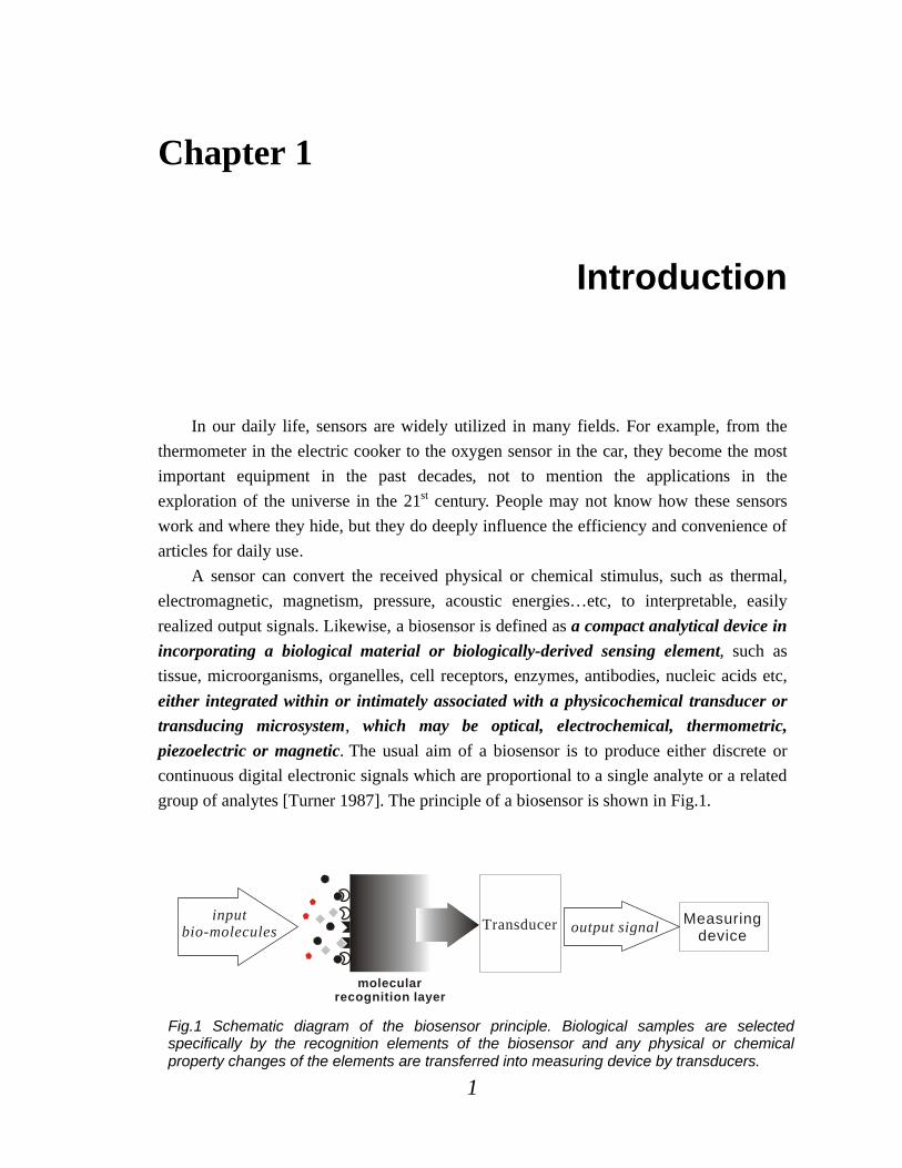


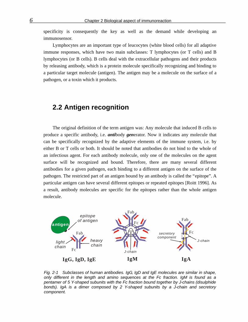
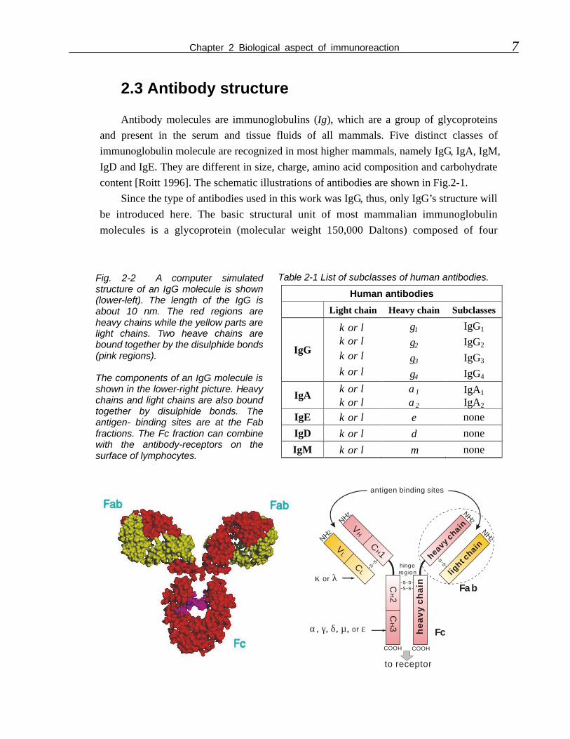


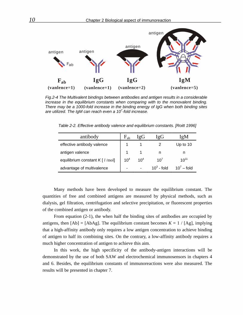

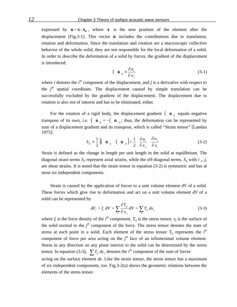


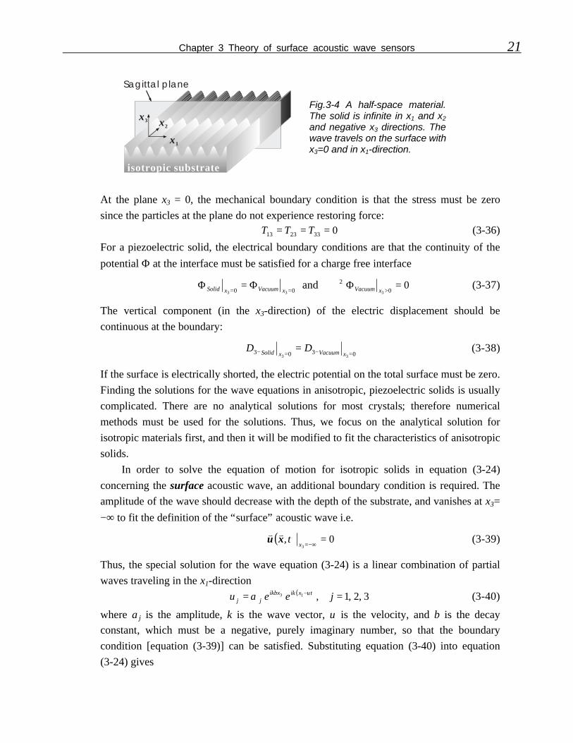

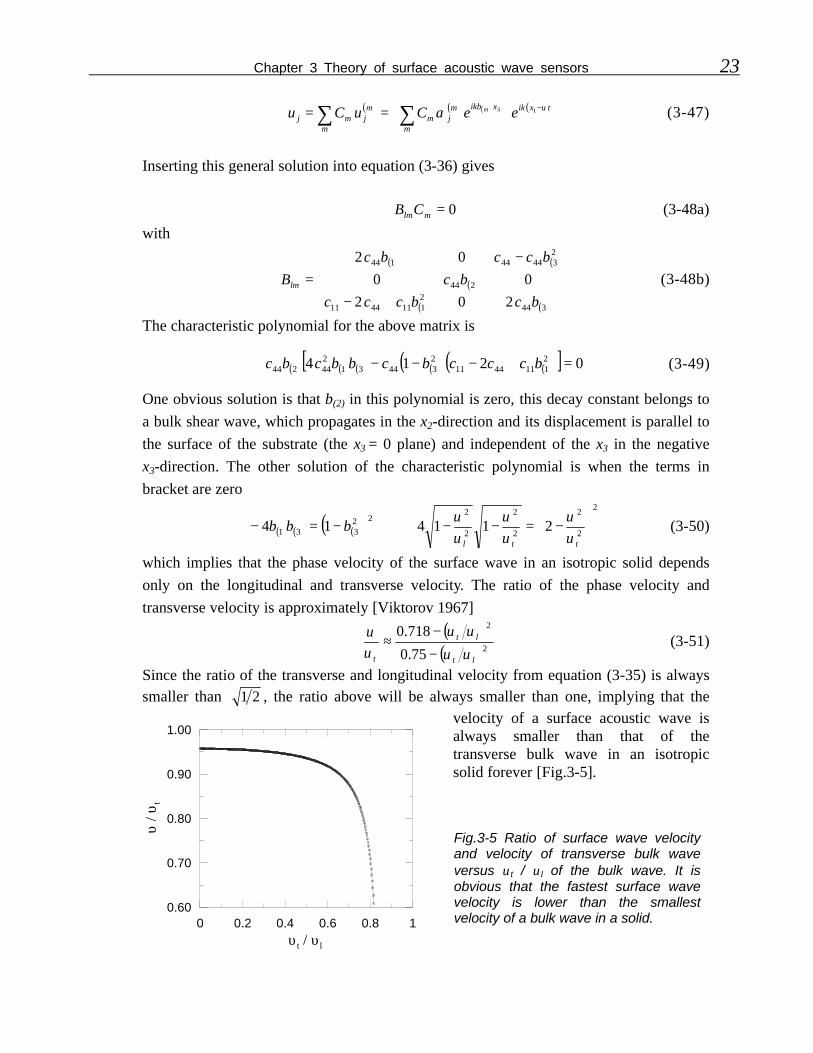


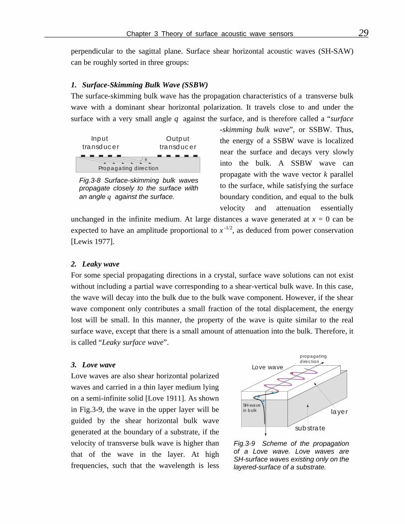

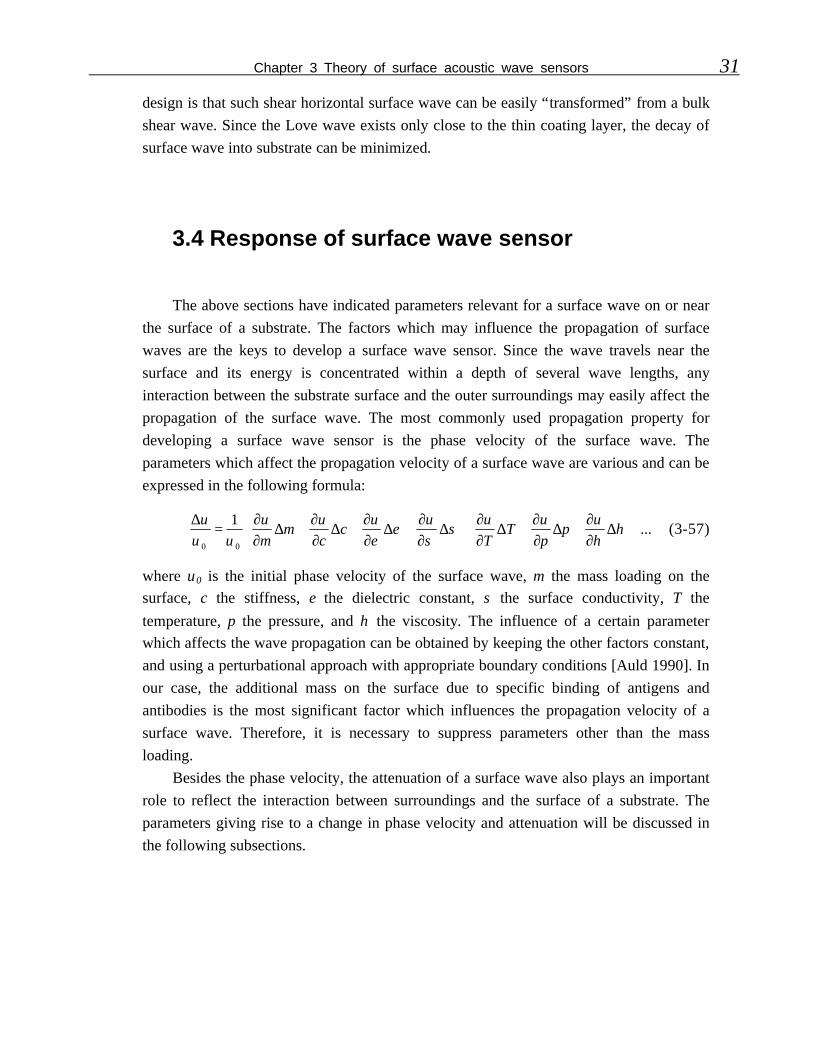


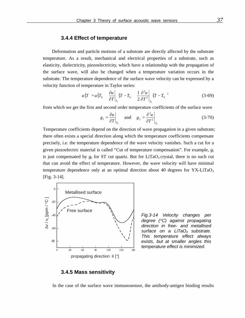

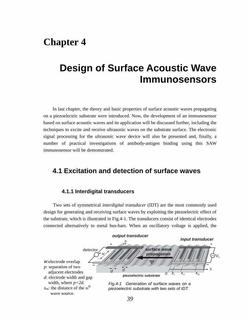


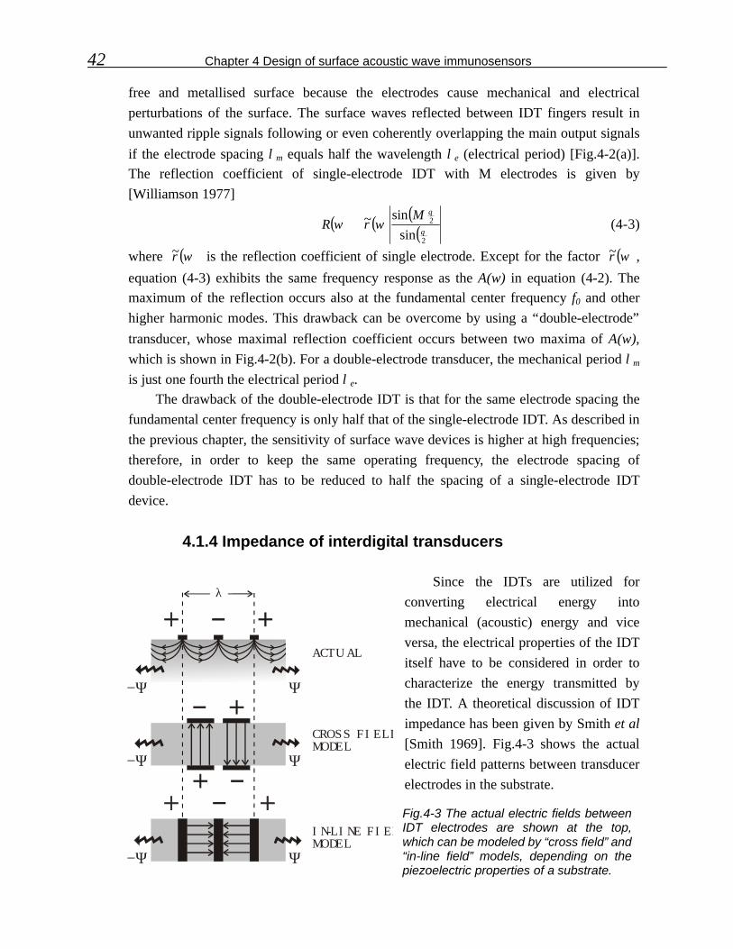
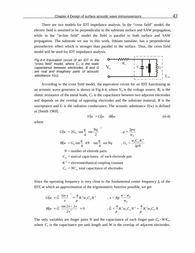
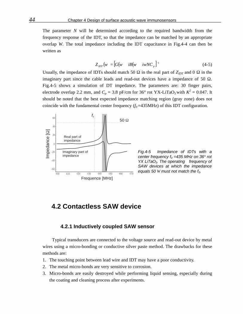
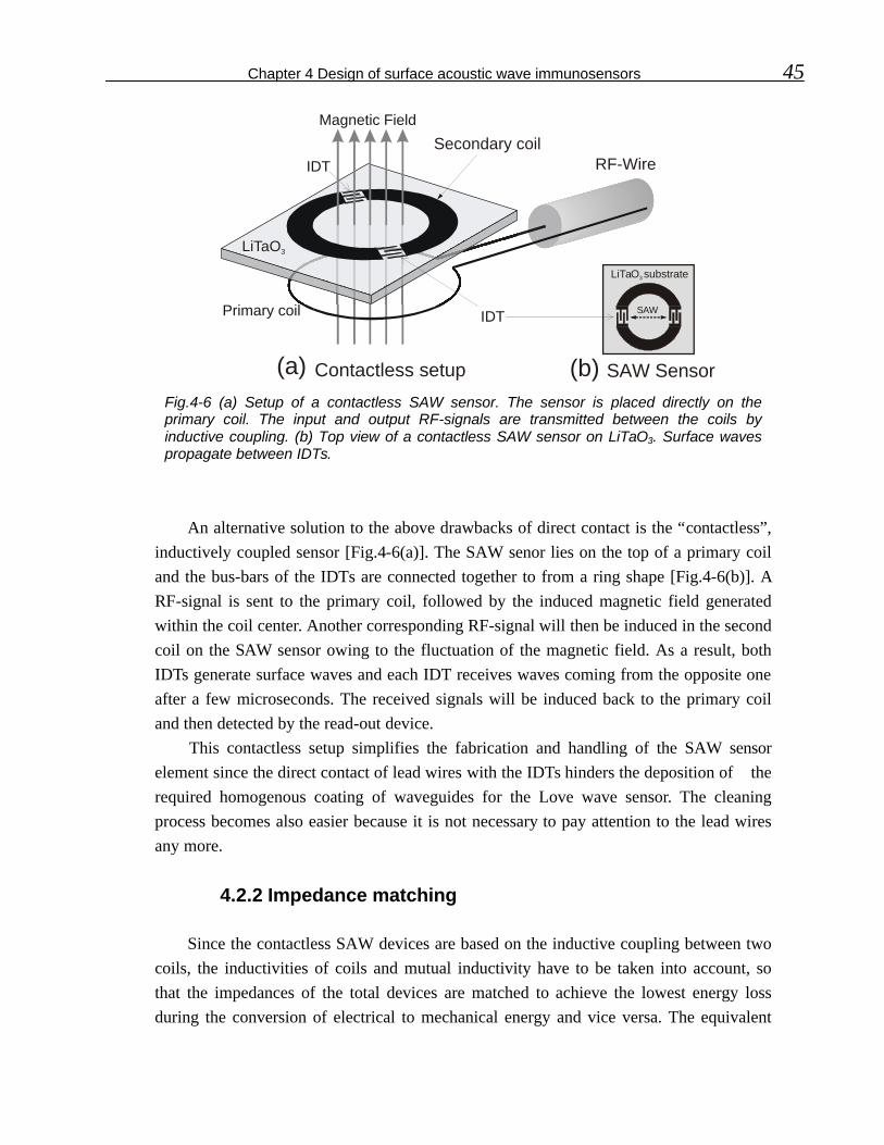


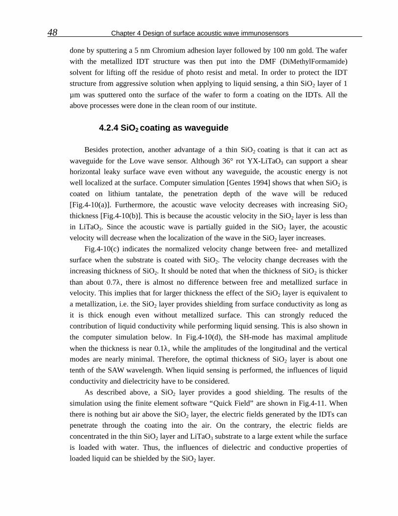


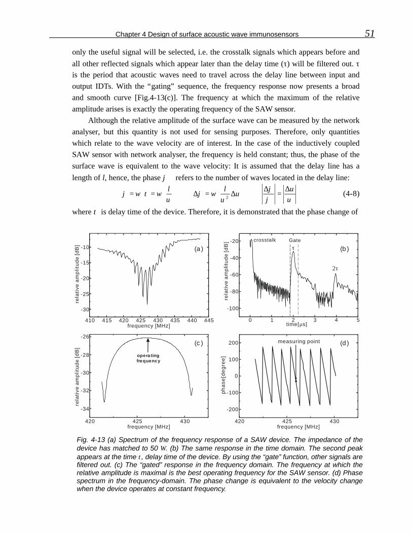
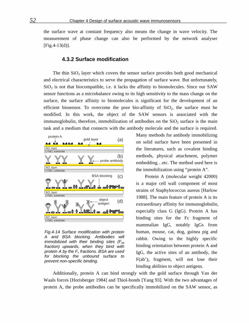


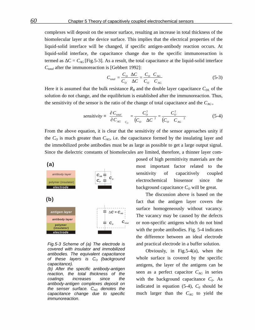


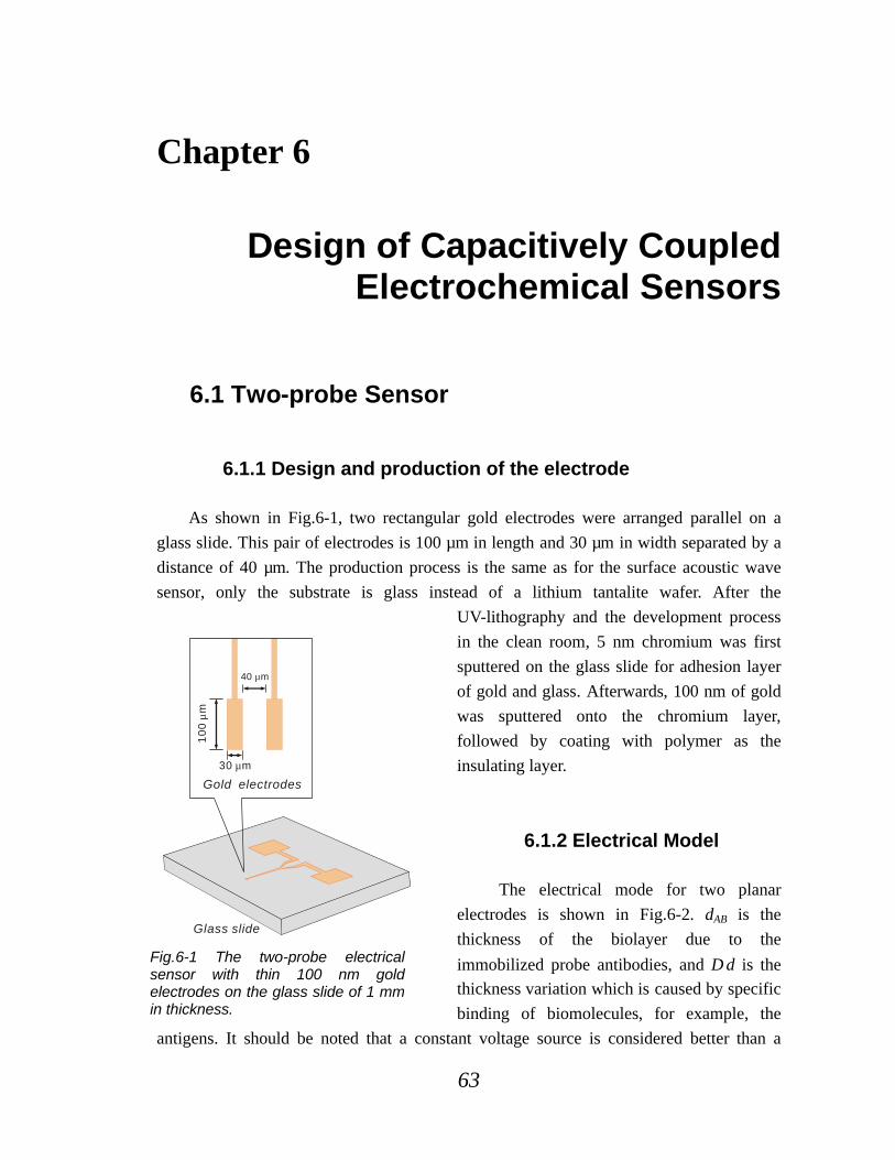


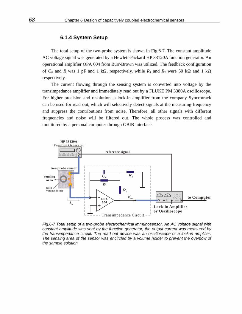


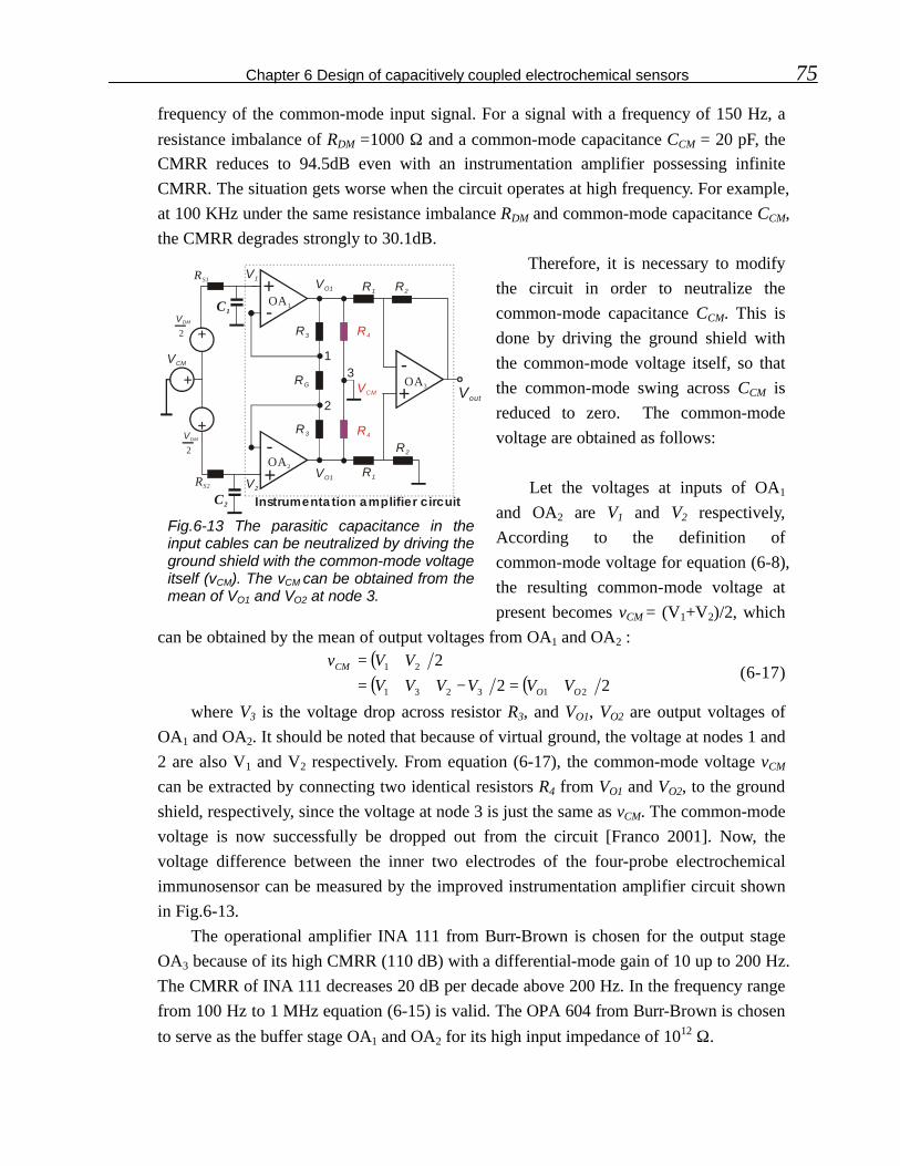


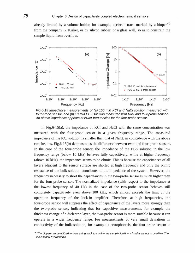


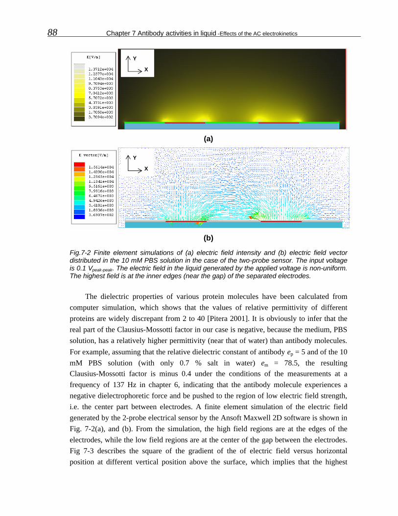


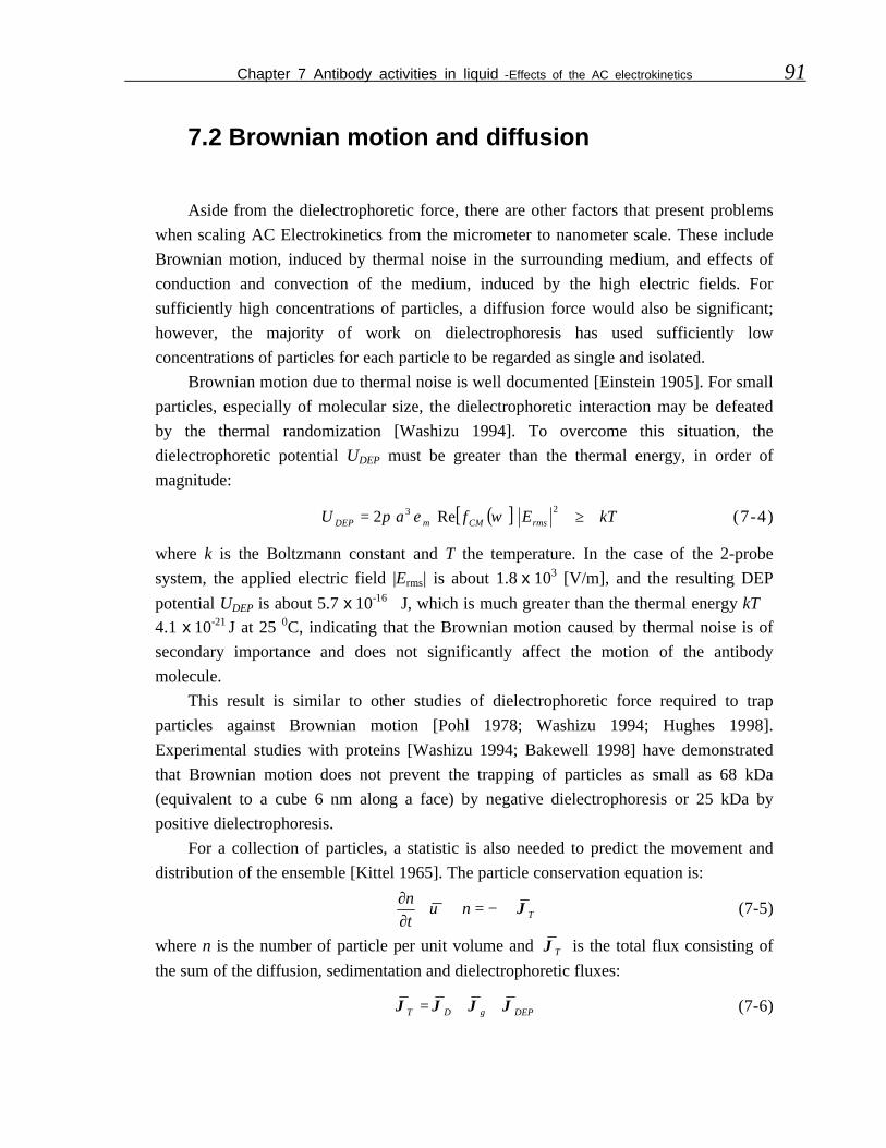


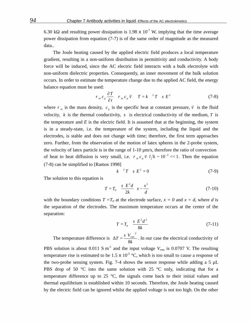
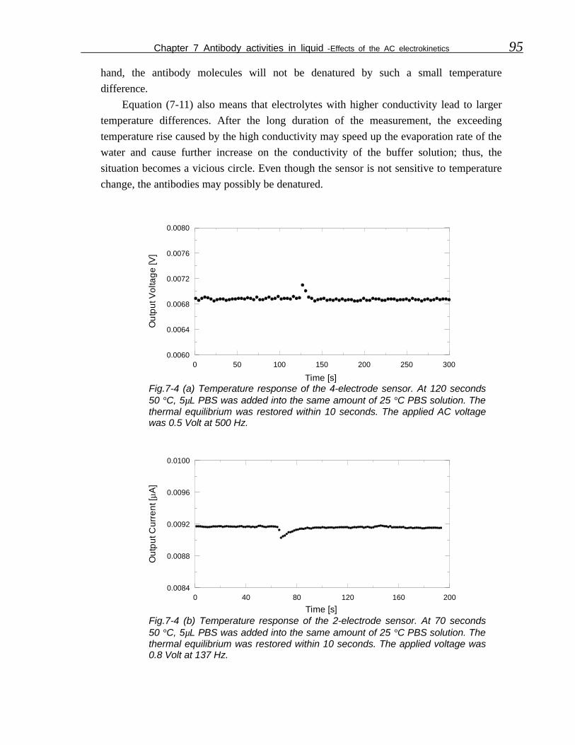


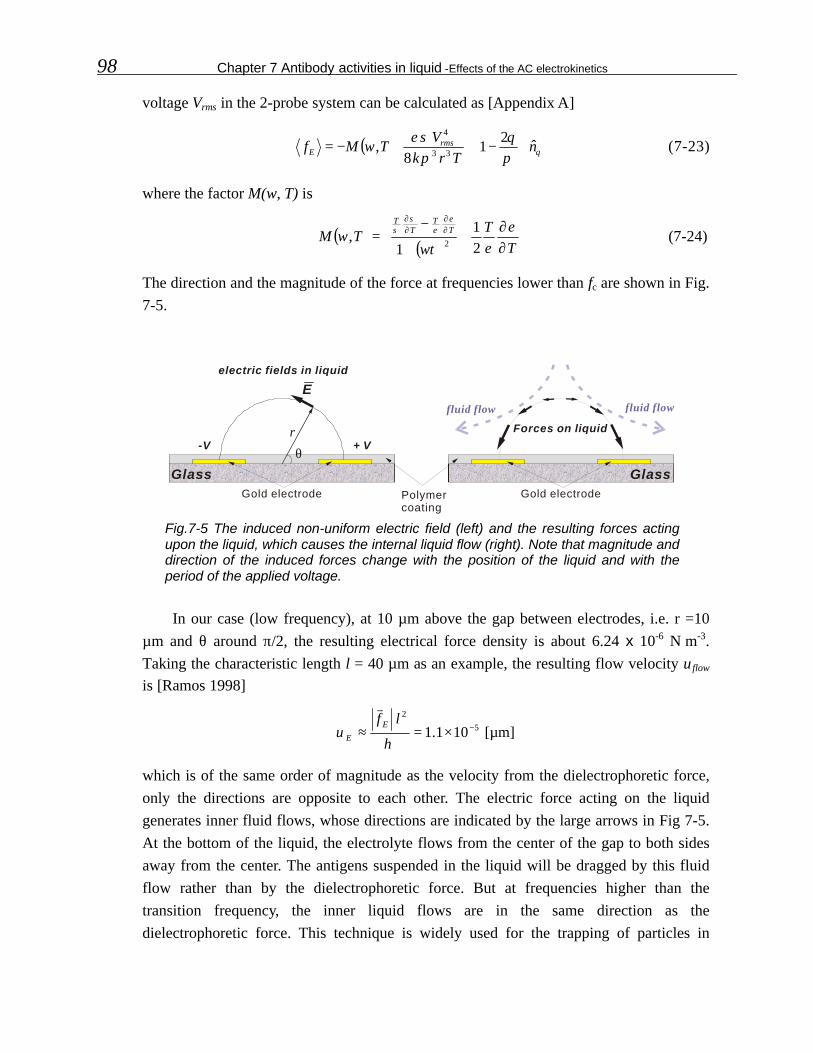
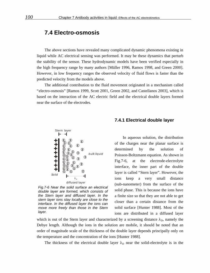
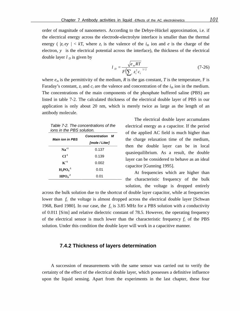
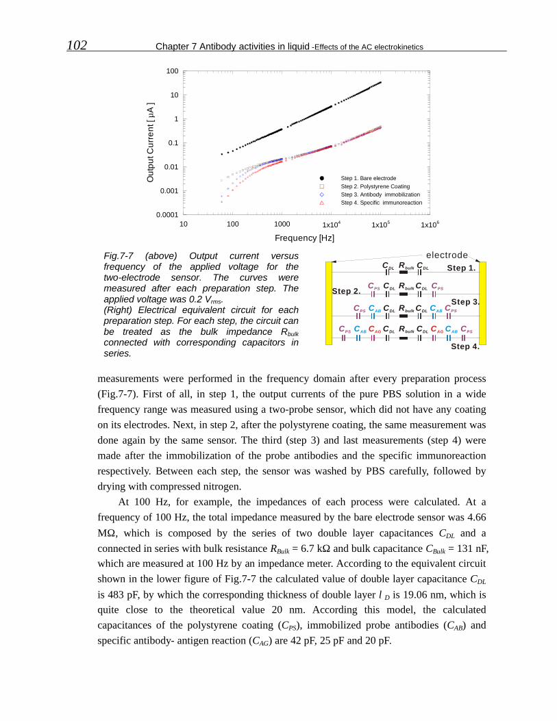
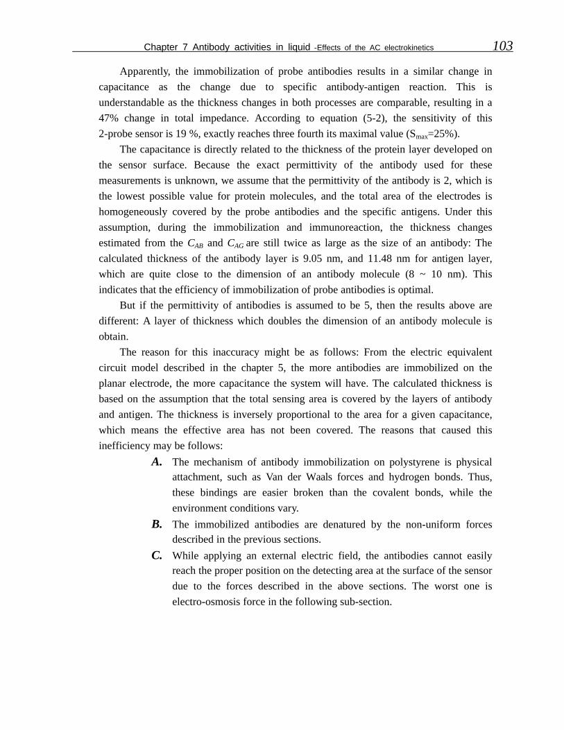
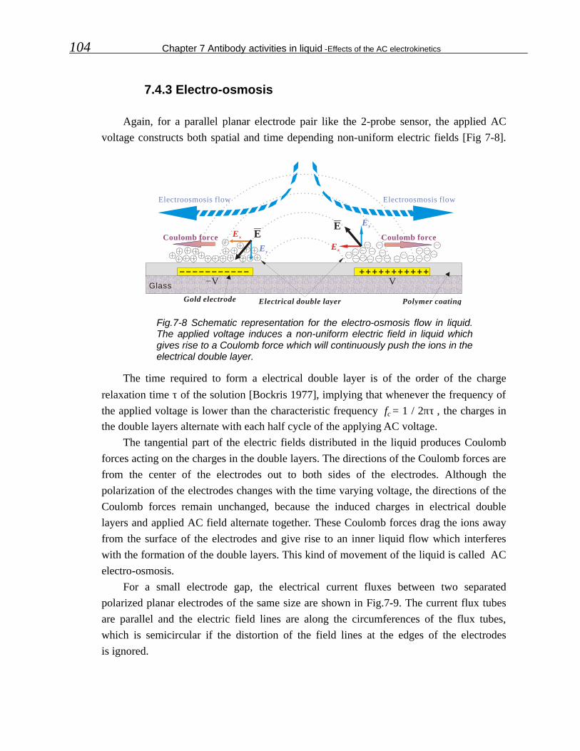
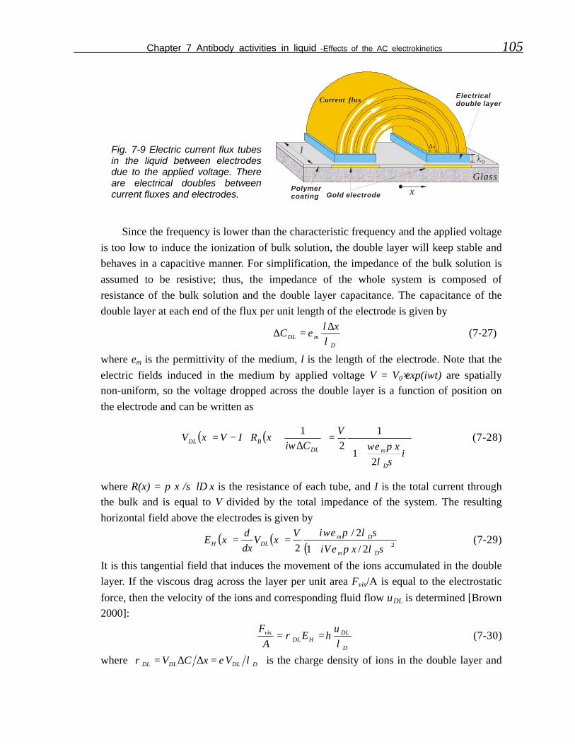

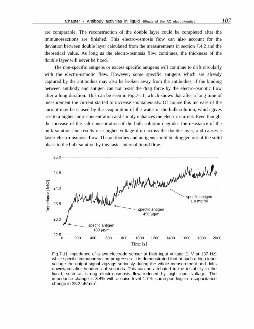

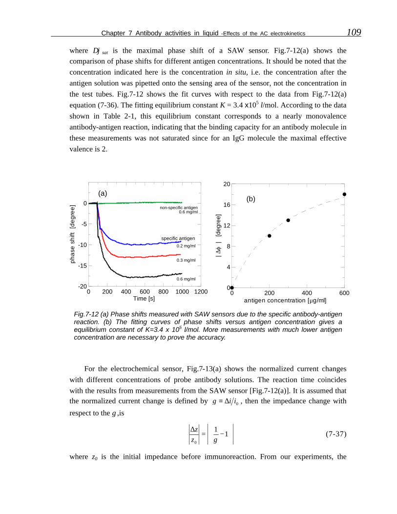


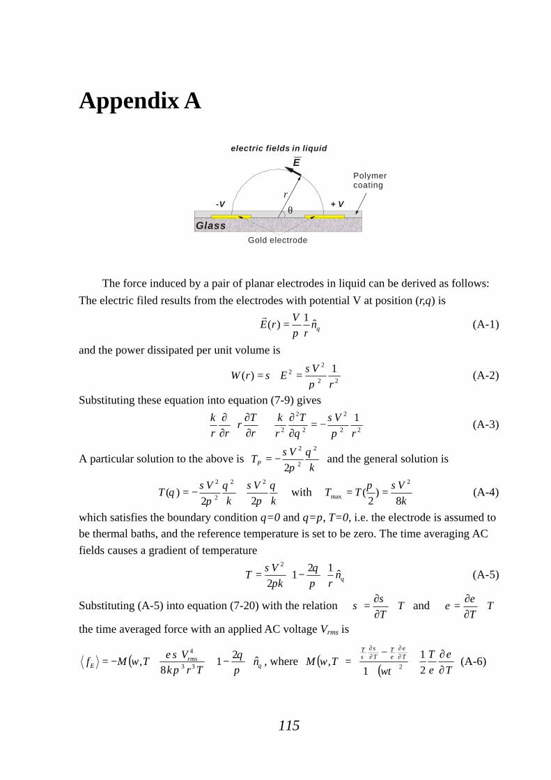


![[ INSIDE PHOTOGRAPHY] - archiv.ub.uni-heidelberg.dearchiv.ub.uni-heidelberg.de/artdok/1566/1/Mueller_Inside_photography... · print. In a very instructive essay, Alexander Liberman,](https://static.documents.pub/doc/80x56/5e1edb3196dfc42a99202245/-inside-photography-print-in-a-very-instructive-essay-alexander-liberman.jpg)


