DISSERTATION PLASMA FLOW FIELD MEASUREMENTS DOWNSTREAM OF A HOLLOW CATHODE Submitted by Casey Coffman Farnell Department of Mechanical Engineering In partial fulfillment of the requirements For the Degree of Doctor of Philosophy Colorado State University Fort Collins, Colorado Fall 2007
Transcript
DISSERTATION
PLASMA FLOW FIELD MEASUREMENTS DOWNSTREAM
OF A HOLLOW CATHODE
Submitted by
Casey Coffman Farnell
Department of Mechanical Engineering
In partial fulfillment of the requirements
For the Degree of Doctor of Philosophy
Colorado State University
Fort Collins, Colorado
Fall 2007
ii
COLORADO STATE UNIVERSITY
October 29, 2007
WE HEREBY RECOMMEND THAT THE DISSERTATION PREPARED
UNDER OUR SUPERVISION BY CASEY C. FARNELL ENTITLED PLASMA
FLOW FIELD MEASUREMENTS DOWNSTREAM OF A HOLLOW CATHODE BE
ACCEPTED AS FULFILLING IN PART REQUIREMENTS FOR THE DEGREE OF
DOCTOR OF PHILOSOPHY.
iii
ABSTRACT OF DISSERTATION
PLASMA FLOW FIELD MEASUREMENTS DOWNSTREAM
OF A HOLLOW CATHODE
The focus of the research described herein is to investigate and characterize the
plasma produced downstream of a hollow cathode with the goal of identifying groups of
ions and possible mechanisms of their formation within a plasma discharge that might
cause erosion, especially with respect to the hollow cathode assembly. In space
applications, hollow cathodes are used in electrostatic propulsion devices, especially in
ion thrusters and Hall thrusters, to provide electrons to sustain the plasma discharge and
neutralize the ion beam. This research is considered important based upon previous
thruster life tests that have found erosion occurring on hollow cathode, keeper, and ion
optics surfaces exposed to the discharge plasma. This erosion has the potential to limit
the life of the thruster, especially during ambitious missions that require ultra long
periods of thruster operation.
Results are presented from two discharge chamber configurations that produced
very different plasma environments. Four types of diagnostics are described that were
used to probe the plasma including an emissive probe, a triple Langmuir probe, a
remotely located electrostatic analyzer (ESA), and an ExB probe attached to the ESA. In
addition, a simulation model was created that correlates the measurements from the direct
and remotely located probes.
Casey C. Farnell Department of Mechanical Engineering
Colorado State University Fort Collins, CO 80523
Fall 2007
iv
ACKNOWLEDGEMENTS
I would like to thank my principle advisors, Dr. Paul Wilbur and Dr. John
Williams, for sharing their expertise, leadership, and encouragement to reach this point in
my research. I would also like to thank my family and friends for their positive and
8.2 Constant Transmission Mode and Variable Transmission Mode ................... 124
9 Appendix C – ExB Probe Equations ................................................................... 129
4
1 Introduction
1.1 Research Goal
In space applications, hollow cathodes are used in electrostatic propulsion
devices, especially in ion thrusters and Hall thrusters, to provide electrons to sustain the
plasma discharge and neutralize the ion beam. Hollow cathodes can also be used as
plasma contactors on spacecraft to manage spacecraft charging. In addition, hollow
cathodes are used in many ground based ion and plasma sources, which are used for
plasma processing applications including ion beam sputtering and deposition. The focus
of this research is to investigate and characterize the plasma produced downstream of a
hollow cathode. The primary goal is to identify groups of ions and possible mechanisms
responsible for their formation within a plasma discharge that might cause erosion,
especially with respect to the hollow cathode assembly. This research is considered
important based upon previous ion thruster life tests that have shown erosion to occur on
cathode and keeper potential surfaces in contact with the discharge plasma (e.g., the
hollow cathode, heater, heater radiation shielding, keeper, and screen grid). The erosion
has the potential to limit the life of the thruster, especially during ambitious missions that
require ultra long periods of thruster operation or high discharge plasma currents.
5
1.2 Nomenclature
Symbol Units Description
A m2 Area
B G Magnetic field strength
σ m2 Electron-ion cross section
λD m Debye length
e C Electron charge, Cx 1910602.1 −
E J or eV Energy
E V/m Electric field
F N Force
I, J A Current
Bk J/K Boltzmann constant, KJx 231038065.1 −
em kg Electron mass, kgx 3110109.9 −
im kg Ion mass
m& sccm Propellant flow rate
en , in #/m3 Electron and ion density
Pt Torr Vacuum tank pressure
φ , V V Voltage potential
q C Ion charge
eT , iT K or eV Electron temperature, ion temperature
v m/s Velocity
6
1.3 Electric Propulsion
1.3.1 Electric Propulsion Background
The main goal of any space propulsion system is to generate thrust to propel a
spacecraft, whether by chemical (rocket) or electrical (electric propulsion) means1,2. In
an electrostatic ion thruster, the thrust, T, is generated by expelling mass from the
spacecraft at a given rate, m& , at an average velocity, U :
UmT ⋅= & Eq. 1.1
Given a spacecraft mission, there is an associated change in velocity, called the
characteristic velocity, ΔV, which is necessary to achieve the desired objectives of the
mission (e.g., a final destination, station keeping for a given duration, rendezvous at
various locations, sample and return, etc.). More ambitious missions require higher
velocity changes. The velocity change can be related to exhaust velocity by the rocket
equation:
⎟⎟⎠
⎞⎜⎜⎝
⎛⋅⋅=Δ
final
initialu m
mUnV ln Eq. 1.2
Here, minitial and mfinal are the initial and final spacecraft masses and nu is the propellant
utilization efficiency. For missions where the ΔV is large, a higher exhaust velocity
allows for a larger fraction of the initial mass to be retained at the end of the mission. Or
in other words, the propellant mass, mp = minitial – mfinal, required by the mission is a
smaller fraction of the total spacecraft mass. The exhaust velocity for a given mission
can be optimized based on the characteristic velocity, power supply specific mass,
propellant usage, and time of flight considerations3. For most ambitious missions
considered within the range of the solar system, the optimal exhaust velocity is in the
7
10,000 to 100,000 m/s range1. Electric propulsion devices can achieve these exhaust
velocities while chemical rockets can not. As a result, electric propulsion can perform
some of these missions with lower initial mass depending upon the amount of mass
required for the power supply system.
Ion thrusters operate with high overall efficiency (nt ~ 60 to 80 %), with much of
the available power going into accelerating the ions to the desired exhaust velocity. The
overall thruster efficiency, nt, is defined using the thrust, T, propellant flow rate, pm& , and
input power, P, as4:
PmTn
pt ⋅⋅
=&2
2
Eq. 1.3
Due to limitations on the power available to most spacecraft, the mass flow rate to an ion
thruster is relatively low, resulting in low overall thrust. Consequently, to achieve large
spacecraft velocity changes, ion thrusters must operate for very long periods of time (on
the order of years) in either continuous or periodic (on/off) modes.
1.3.2 Ion Thruster Considerations
There are three types of electric propulsion thrusters2: 1) electrothermal, 2)
electromagnetic, and 3) electrostatic. Electrothermal propulsion involves the process of
electrically heating the propellant and then expanding the propellant through a nozzle to
produce thrust. These types of thrusters include resistojets, arcjets, and inductively and
radiatively heated devices. Electromagnetic propulsion utilizes a combination of electric
and magnetic fields to produce thrust efficiently. Examples include
magnetoplasmadynamic (MPD), Hall-current, and pulsed plasma thrusters. Electrostatic
propulsion devices, ion thrusters, use electric fields to accelerate ionized particles to
8
produce thrust. This research will focus on hollow cathodes used in ion thrusters (more
specifically the electron bombardment ion thruster), although hollow cathodes are also
used in Hall-current thrusters for the same purpose.
A schematic of the ion thruster is shown in Figure 1.1. The ion thruster works by
ionizing propellant to create a plasma and then accelerating the charged particles to high
velocities to create thrust4,5.
MagneticRings
Hollow Cathode/ Keeper (Anode)
Neutralizer
Discharge Chamber
Discharge CathodeAssembly
Accel GridScreen Grid
Ion Optics
DischargePlasma
e-
e-
Anode
Beam Ions
AnodeSupplyAnodeSupply
ScreenSupplyScreenSupply
AccelSupplyAccel
SupplyNeut.
SupplyNeut.
Supply
+
- +
+
+
-
-
-
IonNeutral atom
Figure 1.1 Ion thruster schematic. The ionized particles generated in the discharge chamber are accelerated by the ion optics to create thrust. An equal amount of electrons are ejected from the thruster neutralizer to maintain charge neutrality.
The plasma is created within the discharge chamber by first drawing electrons
from the hollow cathode. The hollow cathode works by heating a low work function
insert to emit electrons from the surface. The anode is biased positive of the cathode so
9
that electrons from the cathode gain energy and collide with the neutral propellant. A
fraction of the atoms introduced into the discharge chamber through the plenum and
cathode are ionized to form the plasma. A magnetic field is used to confine the electrons
to increase the probability of ionization of neutral atoms.
Some of the ions that are created in the discharge plasma drift toward the ion
optics system. Often the ion optics system is comprised of two grids: the screen grid and
accelerator (or accel) grid. The accelerator grid is biased negative of the screen grid and
plasma so that the ions are accelerated as they pass through the ion optics system. An
example ion optics system is shown in Figure 1.2 along with a schematic of ions being
drawn from the discharge plasma and accelerated from the thruster. The maximum
amount of ion current that can be drawn through each “beamlet” (one screen-accel hole
pair) is determined using the Child-Langmuir law or perveance equation, which takes
into account space charge limitations2,6:
2
23
max_2
94
dV
mqj T
i
ob ⋅
⋅⋅=
ε Eq. 1.4
Where εo is the permittivity of free space, q is the electric charge, mi is the ion mass, VT
is the total voltage applied to the grids, and d is the effective distance between the grids.
To maintain charge neutrality on the spacecraft, an equal number of electrons must be
ejected for each beam ion. This is accomplished using a second electron source, also a
hollow cathode, called the neutralizer that is placed near the ion optics system.
10
Screen Grid
Accel Grid
Direction ofion travel
Figure 1.2 Photograph of an ion thruster grid set7. The ion optics consists of many small apertures (or “beamlets”) through which the ions are accelerated to very high velocities6.
1.4 Hollow Cathodes
In space applications, hollow cathodes are used in electrostatic propulsion
devices, especially in ion thrusters and Hall thrusters, to provide electrons to sustain the
plasma discharge and neutralize the ion beam. Hollow cathodes can also be used as
plasma contactors on spacecraft to reduce spacecraft charging. Also, hollow cathodes are
used in many ground-based ion sources, which are used for processing applications
including ion beam sputtering and deposition.
The purpose of the hollow cathode in an ion thruster is to readily emit a steady
current of electrons over a long period of time. The hollow cathode assembly consists of
the cathode tube, low work function insert, heater, and keeper as shown in Figure 1.3. A
plasma is generated within the hollow cathode by flowing propellant through the cathode
tube and heating the low work function insert to thermionically emit electrons off the
surface. The electrons collide with the neutral atoms within the tube to excite and ionize
11
a fraction of the propellant to create the plasma. The keeper is biased positive of the
cathode to draw electrons from within the cathode and into the main discharge chamber.
The mechanism of electrons being emitted from the insert surface is called field-
enhanced thermionic emission. The cathode generally operates around 1000 degrees
Celsius to ensure sufficient electron emission from the low work function insert8. During
cathode startup, the required ignition temperature is reached using a heater that is coiled
around the cathode tube. Once the discharge is initiated, the cathode and insert
temperatures are maintained through surface heating from the intense plasma produced
within the cathode tube and the heater power can be turned ‘off’. In addition to heating
the cathode insert, the intense plasma forms a thin sheath just above the insert surface that
results in a strong electric field. The field enhancement process serves to further lower
the effective work function and ensure that the insert surface can emit the demanded
electron current.
In a conventional hollow cathode, the electron insert consists of a porous tungsten
tube that is impregnated with a mixture of barium calcium aluminate (BaO, CaO, and
Al2O3). Ba and BaO from the impregnate rise to the insert surface and coat it resulting in
a dramatically lower work function compared to the work function of a porous tungsten
surface. Two standard impregnate mixtures used most often to fill the pores in the
tungsten insert are Ba4CaAl2O8 and Ba6CaAl4O13, also known as 411 and 612,
respectively, because of their relative molar ratios [i.e., 4(BaO), 1(CaO), and 1(Al2O3)
and 6(BaO), 1(CaO), and 2(Al2O3)]. Newer impregnate combinations and insert
materials being used and considered for cathode inserts include barium scandate,
tungsten-iridium, and lanthanum hexaboride (LaB6)9.
12
There are a few failure modes that have been identified for the hollow cathode
assembly. They include erosion to the orifice and surfaces, insufficient supply rate of
barium, insert poisoning, and tungsten transport to undesired regions10. The focus of this
research is to investigate hollow cathode sputter erosion, which is thought to be primarily
caused by ions generated downstream of the hollow cathode in the discharge plasma.
-
-
-+
Neutral Xe AtomsXe IonsElectrons
+-
Propellant Flow
Heater Coils
Insert – Low work function
- +-
--
+-
-
- +-
--
--
Keeper Tube
Cathode Tube
+-
Figure 1.3a Diagram of the hollow cathode. Electrons are emitted from the low work function insert to sustain the plasma.
Figure 1.3b Hollow cathode, insert, and front view with the enclosed keeper.
1.5 Cathode Erosion and Engineering Solutions
1.5.1 Importance of Hollow Cathode Erosion
Discharge cathode erosion has been identified as one source of life limiting failure
of ion thrusters in space missions11,12. As missions become more ambitious, thruster
lifetime requirements increase based on the time to thrust to achieve the desired change in
velocity, ΔV. Extensive ground and in-space testing has been performed on the NSTAR
ion thruster, which demonstrated an in-space firing sequence of 16265 hours in duration.
13
Ground based tests on the NSTAR thrusters and similar derivatives have consisted of
operational periods of 1000 hours, 8200 hours, and an extended life test that ran for over
30000 hours. Cathode erosion was observed in all of these life tests. Other high current
cathode validation tests have shown much more severe erosion to the cathode assembly
after shorter periods of operation (500 to 2000 hours)13,14,15. Figure 1.4 shows erosion
that occurred to the hollow cathode keeper on an NSTAR thruster during the extended
life test16.
Figure 1.4 Pictures of the discharge cathode assembly at different times on the NSTAR extended life test thruster. The keeper orifice enlarged over time, presumably from ion bombardment from ions produced in the plasma downstream of the cathode orifice16.
With ion bombardment from the plasma, the keeper, cathode, and eventually
heater eroded due to sputtering16. In time, the heater could erode to the point where the
heater filament opens. Once this occurs, the discharge cathode could no longer be started
because the temperature (~1000 degrees Celsius) required to re-start the cathode could
not be achieved.
1.5.2 Engineering Solutions
The effects of erosion to a hollow cathode assembly can be mitigated in several
ways. One engineering solution to reduce cathode orifice plate erosion was to add an
enclosed keeper11. The orifice plate of the enclosed keeper structure acts to shield the
cathode and heater from direct bombardment from plasma ions. The enclosed keeper
14
allows for longer lifetimes because the keeper acts mostly as a sacrificial element once
the cathode is operating. An increased lifetime could come from a thicker keeper plate as
long as the potential profiles (temporal and spatial) around the cathode are not adversely
affected.
Another engineering solution to increase cathode lifetimes is to modify the
cathode assembly materials so that they are more resistant to sputtering. Similar to
material selection for ion thruster optics design, carbon/graphite has been considered as
an improvement to molybdenum based on lower sputter yield rate predictions of
graphite7. Tantalum is another material that has been considered for keeper use due to
low sputter yield characteristics in comparison to molybdenum16.
A more useful (however more difficult) solution would be to modify the plasma
characteristics near the hollow cathode, since cathode erosion is most likely caused by
sputtering from ions, sometimes highly energetic, that are produced within the discharge
plasma17. This is the focus of the research presented herein. There are a few ways
erosion could be reduced including 1) reduction of the local plasma potentials and
thereby energy of the ions produced near the cathode and/or reduction of the production
rate of multiply charged ions near the cathode, 2) reduction of the plasma density
produced near the cathode, or 3) re-direction of ions that are produced nearby the cathode
to regions away from the cathode. All of the above (if possible) may involve a
combination of changes to the ion thruster such as the discharge chamber geometry,
cathode geometry, keeper geometry, magnetic field strength and geometry, cathode flow
rate, main discharge flow rate, keeper current, discharge current, etc.
15
1.5.3 Sputtering
The erosion of the cathode assembly is based upon the relationship between the
plasma properties and how ions from the plasma impact the cathode. Sputtering is an
extensive field of study and has many applications outside of electric propulsion. The
largest field is in material processing, such as semiconductors, where ion beams are used
to sputter, implant, and etch the surface of materials to achieve desired surface qualities
and material coatings.
Sputtering, which is an area of interest in regard to hollow cathodes and this
research, involves the process of removing material from a surface as a result of particle
impact18. When an energetic ion hits a surface there is a certain probability that atoms
will be ejected, or sputtered, from the surface. The total sputter yield, Y, is defined as the
number of atoms ejected from the surface per incoming ion. Major factors that affect the
sputter yield are the ion energy, ion species, incidence angle, and the target species and
surface properties. An example sputter yield curve is shown in Figure 1.5 for xenon
atoms striking a molybdenum target at an incidence angle of 0 degrees19. The sputter
yield increases as the ion energy impacting the surface is increased. From knowledge of
the plasma properties and surface variables, the erosion rate could be calculated. The
erosion rate gives an estimate for how long a material, such as a keeper plate or cathode,
would last when exposed to the plasma.
16
1.E-07
1.E-06
1.E-05
1.E-04
1.E-03
1.E-02
1.E-01
1.E+00
0 10 20 30 40 50 60 70 80Energy (eV)
Spu
tter Y
ield
, Y (a
tom
s/io
n)
Xenon on MolybdenumIncidence = 0o
Figure 1.5 Example sputter yield curve for xenon atoms striking a molybdenum target at an incidence angle of 0 degrees (curve fit of data from ref. 19).
1.6 Proposed Mechanisms for Accelerated Erosion
Ions that are created in a plasma can sputter erode the surfaces of the cathode
assembly11,15. The erosion rate of the cathode and keeper could increase if the energy of
the incoming ions is increased or if the flux of ions is increased. Therefore, it is of
interest to not only investigate how the cathode components are eroded, but to investigate
possible mechanisms which cause the higher than anticipated erosion rates that are
observed in some tests. The following sub-sections describe possible mechanisms that
could cause increased erosion of the hollow cathode/keeper assembly.
1.6.1 Potential Hill Model
The potential hill theory was proposed to explain how ions could be created that
have the ability to quickly erode materials within the discharge chamber, especially near
the hollow cathode. The idea is that a steady (DC) potential hill could be formed just
downstream of a hollow cathode that would serve to generate energetic ions (once they
17
fall from their point of origin to a cathode and keeper surface). Various research, such as
that from Friedly17, Williams and Wilbur20, Kameyama and Wilbur21, Crofton and
Boyd22, and Katz et al.23, have proposed that such a potential hill could exist given the
relative speeds and densities of electrons and ions that are created in the high density
plasma. The size and shape of the potential hill, and therefore the resulting energies of
ions from the region, would change depending on the discharge chamber geometry, flow
rate, discharge voltage, and discharge current. Other areas of research have also looked
at potential hills. One example is Hantzsche24 who discussed a model for hydrodynamic
drag in vacuum arcs in which a potential hump (or hill) exists near the cathode arc point.
In this model, forces from electric fields, pressure gradients, and electron-ion friction
were considered to act on the ions and electrons.
1.6.2 Magnetohydrodynamic Effect – MHD Effect
The MHD theory involves the effects of electron currents flowing through the
hollow cathode orifice. The idea is that the electron flow from the cathode produces a
self-induced magnetic field, which then yields a Lorentz force. However, Kameyama25
indicated the energy gain from the force would be relatively small for the cathodes
considered (~ 0 to 1 eV), indicating that this effect would not cause significantly higher
ion energies to be produced near the cathode.
1.6.3 Orifice Causes (Orifice Wall Kinetic Energy Collisions)
Foster and Patterson26 investigated ion energy distribution functions in a hollow
cathode discharge plasma environment similar to research performed at Colorado State
University. Electrostatic analyzer (ESA) measurements of the discharge plasma showed
18
ion energy distribution functions with a wide spread of energies including energetic ion
tails. One idea proposed by Foster and Patterson was that energetic ions could be
produced within the hollow cathode orifice by multiple ionization reactions occurring
within the orifice combined with finite fractions of left-over kinetic energy from glancing
wall neutralization events. This theory does not agree well with experimental
measurements because large numbers of energetic ions are observed at large off-
centerline angles, and because erosion is detected on the downstream surface of the
Both Domonkos and Williams11,27 and Herman and Gallimore28 compared
measured erosion rates from the 1000 hour and 8200 hour tests of the NSTAR discharge
chamber to simple sputtering models. The models used values for the ion energies, ion
current densities, and ion incidence angles that were derived from experimental
measurements, and an assumed fraction of doubly charged ions (5 to 20 %) that might
exist near the hollow cathode. The estimated erosion rate came close to the observed
erosion rate considering the uncertainties in sputter yields at low energies. Since the
doubly charged ions were observed to cause nearly all of the cathode erosion, this theory
implies that ions with energies above the cathode to anode potential do not play a
significant role in cathode erosion, especially for the conditions found within the NSTAR
discharge chamber. In addition to the researchers mentioned above, recent work from
Herman and Gallimore29, Goebel et al.30, and Martin et al.31, have measured DC potential
wells directly in front of the hollow cathode. Ions produced within the potential well
would be channeled toward the cathode assembly if a low potential path existed from the
19
potential well region to the cathode. However, unless these ions were multiply charged,
they would not strike the cathode assembly surfaces with significant energy to sputter.
1.6.5 Potential Well (Charge Exchange)
Katz et al.32 have proposed a possible mechanism for the formation of energetic
ions that involves charge exchange neutralization near the hollow cathode. The idea is
that ions will alternately gain kinetic energy and then potential energy by going through a
charge exchange process within a potential well that exists near the hollow cathode. In
addition to the DC potential well, this idea can be combined with potential structure
oscillations to produce ions with energies higher than the cathode-to-anode voltage
difference. Calculations of potential profiles and estimates of plasma properties were
made to combine the theory with RPA measurements made at remote axial and radial
locations from a hollow cathode experiment. Although this work is promising, Katz et
al.32 point out that most of the ions would not be directed toward the cathode assembly
and therefore might not be critical in affecting cathode erosion.
1.6.6 Oscillations / Turbulent Ion Acoustic Waves
In a discharge, it is common to have plasma oscillations due to the counter
streaming currents of ions and electrons and due to steep gradients in plasma production
rates. Oscillations based on these processes have been observed in Hall type thrusters as
well as in ion thrusters33. For example, noteworthy discharge voltage oscillations of
about 5 to 10 V peak-to-peak were measured in an NSTAR-like discharge by Domonkos
and Williams11 compared to the DC discharge voltage which was around 25 V.
Oscillations of this magnitude can be present in the discharge plasma flow fields as well,
20
especially for operation at high discharge current, high discharge voltage, or low flow
rate conditions. As an example, large amplitude plasma potential oscillations (~ ±20 V)
were observed nearby a hollow cathode at some operating conditions by Goebel et al.30
that could produce ions with energies well above the cathode-to-anode voltage. These
large amplitude oscillations appeared to be present especially for lower magnitude
magnetic field strengths. The presence of potential oscillations could increase sputter
rates of cathode components, due to increased bombarding ion energies from ions created
at higher potentials. Mikellides et al.16 estimated an erosion rate of the keeper surface
from the 8200 hour NSTAR Life Demonstration Test considering the effects of plasma
potential oscillations. Assuming that singly charged ions sputter eroded the surface of the
cathode (i.e., no doubly charged ions were assumed to be present), Mikellides et al. found
better agreement with the experimental measurements when including the effects of high
potential oscillations that would accelerate ions to higher energies and induce higher
sputter erosion rates.
1.7 Investigation Summary
In view of the cathode life tests which showed erosion to the cathode assembly as
well as the proposed models that identify possible mechanisms of erosion to the cathode
assembly, the focus is to further investigate and characterize the plasma produced
downstream of a hollow cathode. Measurements using a variety of diagnostic tools in
different discharge configurations will help to identify important ion groups and
formation regions for investigation of cathode erosion mechanisms.
21
2 Experimental Setup and Diagnostic Tools
This section describes the vacuum facility, discharge chamber configurations, and
diagnostic tools that were used to probe plasmas. Two discharge chamber configurations
were used that had different geometries, which resulted in very different plasma
environments. In both cases, the same hollow cathode was used to produce and sustain
the plasma. Four types of diagnostics were utilized to probe the plasma; an emissive
probe, a triple Langmuir probe, a remotely located electrostatic analyzer (ESA), and an
ExB probe (or Wein filter) attached to the ESA.
2.1 Vacuum Facility
All tests were performed in a 1.2 m diameter by 4.6 m long stainless steel vacuum
chamber that was pumped with a 0.9-m diameter, 20-kW diffusion pump. The base
pressure of this facility with no flow was 1x10⁻⁶ Torr after a 2 hr pump down time. The
vacuum pressure was in the low to mid 10-5 Torr range at typical xenon flow rates of 3 to
15 sccm.
2.2 Case 1: Open Cathode (Zero Magnetic Field) Configuration
A picture of the open cathode configuration is shown in Figure 2.1. The cathode
assembly was set up in the center of a stainless steel ring anode. Here, electrons were
drawn from the cathode assembly to the ring anode without any other discharge chamber
structure present. No magnet rings were used in this configuration. The anode was
19.5 cm in diameter and 9 cm in length. This configuration was beneficial in that the
plasma was easily accessible by both emissive and triple Langmuir probes (for direct
measurement) and by the remotely located ESA and ExB probes.
22
19.5 cm
9 cm
0.5 cm
Figure 2.1 Open cathode (zero magnetic field) configuration. The anode was 19.5 cm in diameter and 9 cm in length.
2.3 Case 2: Prototype NSTAR Discharge Chamber Configuration
The second experimental setup consisted of a hollow cathode mounted within a
discharge chamber as seen in Figure 2.2. The discharge chamber had a 30-cm diameter
cylindrical section attached to a conical central section which was capped by a back plate
and was, therefore, similar in size, shape, and magnetic field geometry to the NSTAR
thruster34,35,36,37,38. The discharge chamber was made from sheet aluminum with an inner
stainless steel lining and three magnet (samarium cobalt) rings. The first ring was located
near the exit of the source (where the ion optics would be located on an actual NSTAR
ion engine) at one end of the cylindrical sidewall section, the second was placed at the
intersection of the cylindrical and conical anode sections, and the third behind the
cathode on the back plate. A more detailed layout of the magnetic field and relative field
strengths is discussed in Appendix A. A pseudo-screen grid fabricated from stainless
steel and biased to cathode potential was used to simulate the neutral flow restricting
23
behavior of an actual ion optics system. Ions produced in the plasma were allowed to
flow directly from the discharge chamber through a 6 mm wide slot cut in the side wall of
the discharge chamber and pseudo-screen grid so they could be sensed by remotely
located probes. The discharge chamber/hollow cathode system was mounted within a
fixture so that it could be rotated about an axis centered at the cathode orifice thereby
enabling measurements at angles from 0o to 90o with respect to the cathode centerline.
This was done to investigate the size and shape of the dense plasma region produced near
the hollow cathode orifice.
Magnet rings
Pseudo-screen grid
Hollow cathode assembly
Magnetic field lines
Anode Figure 2.2a Side view of the prototype NSTAR discharge chamber.
Figure 2.2b Discharge chamber schematic.
2.4 Cathode/Keeper Assembly
The cathode/keeper assembly is shown in a side view and in a view along the
cathode axis looking down the orifice in Figure 2.3. The same cathode and keeper was
used in both case 1 and case 2 configurations. The hollow cathode was a 6.3 mm
diameter tube that contained a low-work-function impregnated, sintered tungsten insert.
The hollow cathode tube was capped with an orifice plate that had a 0.55 mm diameter
orifice on its centerline. The cathode tube and insert were heated by a resistive coil
24
wrapped around the outside of the tube, which was insulated by a multiple-layer,
tantalum-foil radiation shield. The enclosed keeper used with the cathode was equipped
with an orifice plate fabricated from 0.635 mm thick tantalum. The keeper orifice plate
had a 2.54 mm diameter orifice positioned about 0.5 mm downstream of the cathode
orifice plate. It is noted that the cathode and keeper orifice diameters were similar to but
not exactly the same as the discharge cathode and keeper features used in the NSTAR ion
thruster. All of the xenon propellant required to operate the cathode and the discharge
chamber plasma were supplied through the cathode. In case 2, because high voltages
were not applied to extract ions and propellant was lost only through the relatively small
slot in the chamber side-wall and the pseudo-grid surface, the flow through the cathode
was sufficient to produce NSTAR-like neutral densities throughout the discharge plasma.
Figure 2.3 Cathode and keeper assembly with close-up front view of the keeper and cathode orifices.
2.5 Remote Probes – ESA, ExB
2.5.1 Electrostatic Analyzer (ESA)
A Comstock model AC-901 electrostatic analyzer (ESA), shown in Figure 2.4,
was used to measure the energy of the plasma ions39. The ESA consisted of two
25
spherical sector plates fabricated in a 160o arc. Two collimators were used at each end of
the arc to limit the field of view of the device. Both collimators were comprised of a set
of two disks with 2 mm holes aligned with each other and separated by 1 cm. A nickel
mesh was placed in front of the entrance aperture to shield the ESA from ambient plasma
electrons that might penetrate the collimator assembly and flow around the spherical
sectors to the collector electrode. The collector electrode was located downstream of the
exit collimator and was well isolated from the plasma to ensure accurate current
measurements. In order to collect all of the ions that passed through the ESA on the
proper trajectories, a small negative DC bias was applied to the collector electrode to
draw those ions to it. A computer was used to control a Keithley 617 programmable
electrometer that applied both the desired potentials to the spherical plates through a
resistive voltage divider circuit relative to the entrance and exit collimators and measured
the ion current flowing to the collector. The voltage difference on the spherical plates
was converted to ion energy (actually ion energy per charge state, E/z) using Eq. 2.139:
2
1
1
2
rr
rrz
E−
Δ=
φ or, for the ESA geometry used: φΔ*2.254E =z Eq. 2.1
In Eq. 2.1, E represents the ion energy, z the ion charge state (i.e. z = 1 for singly charged
ions, z = 2 for doubly charged ions, etc.), r1 and r2 the inner and outer radii of the ESA
spherical segments, and Δφ the voltage difference applied between r1 and r2. Note that
the ESA detected only the energy to charge ratio, E/z, so a singly charged ion and a
doubly charged ion that went through a potential ΔVp would be measured at the same Δφ.
Once the voltages were applied to the segments, a picoammeter built into the Keithley
electrometer was used to measure the ion current that flowed to the collector electrode.
26
Segments
Collimators
Collector
φ1
r1
r2
rm
φ2
ΔVpsegE
Figure 2.4a Picture of the ESA with the top cover removed.
Figure 2.4b Diagram of the ESA.
There are two modes of ESA operation that can be used to measure an ion energy
distribution function (IEDF); the variable transmission energy mode (or sector field
sweep mode) and the constant transmission energy mode39. While both modes of
operation were used in this work, it was decided that the constant transmission energy
mode was more suitable. When presenting data obtained with the ESA, the reader can
assume that the constant transmission mode was used unless otherwise noted. In the
constant transmission mode, a constant Δφ was applied between the segments, and the
entrance and exit collimators were swept (along with the segments) with respect to the
vacuum facility ground to yield the ion energy distribution function. Figure 2.5 shows an
example ion energy distribution function generated with the ESA. The current to the
collector plate was recorded as a function of the bias voltages, which determined the
selected ion energy to charge ratio (E/z). Appendix B discusses the ESA modes of
27
operation in further detail as well as the governing equations for the relationship between
the ESA geometry and the measured ion energies. For both case 1 and 2 configurations,
the cathode was grounded to the vacuum test facility wall.
0
10
20
30
40
50
0 10 20 30 40 50 60 70 80 90 100ION ENERGY (eV)
ION
CU
RR
EN
T (n
A)
Electrostatic Analyzer (ESA)
VD = 25 V, JD = 25 A
Figure 2.5 Example ion energy distribution function (IEDF) measured with the ESA.
2.5.2 Combined ESA_ExB Probe
The combined ESA and ExB probe was used to measure the energy and charge
state of the plasma ions. The probe consisted of an ExB stage mounted onto the exit
stage of the Comstock model AC-901 ESA39, as shown in Figure 2.6. With this setup, an
ESA trace could be taken to obtain an ion energy distribution function (E/z) by using the
ExB probe collimator as an ion collector plate. Alternately, the ExB probe could be used
to measure the charge state distribution when the ESA was set to transmit a given ion
energy.
28
ExB Probe
ESA
Probe Entrance
ESA Collector/ExB Collimator
Prototype NSTAR Discharge Chamber
ESA Section(Energy Selection)
ExB Section(Charge State)
Prototype NSTAR Discharge Chamber
ESA Section(Energy Selection)
ExB Section(Charge State)
Figure 2.6a Combined ESA_ExB probe. The ESA section is used to select ions according to their energy to charge ratio (E/z) and the ExB section is used to separate ions of different charge (z).
Figure 2.6b ESA_ExB probe looking toward the prototype NSTAR discharge chamber (case 2) at a zenith angle of 90 degrees.
The ExB probe (or Wein filter) is used to measure the charge state of the ions via
crossed magnetic and electric fields that separate the ions41,42. The ExB probe schematic
is shown in Figure 2.7. Ions that are able to pass through the collimator enter the
separation region where they feel a force from both the electric and magnetic fields
according to the Lorentz force equation:
)( BvEqF ×+⋅= Eq. 2.2
In Eq. 2.2, F represents the force on the ion, q the electronic charge, E the electric field
strength, v the ion velocity, and B the magnetic field strength. In order to pass through
the probe to the collector plate, the net force on the ions must be near zero so that the ions
are not pushed off the drift axis. The resulting equation for the ions that are measured by
the ExB probe is:
22
2
2 BdqzmVP ⋅⋅⋅⋅
Δ⋅=Δ
φ Eq. 2.3
29
In Eq. 2.3, ΔVp represents the potential difference between the ion creation potential in
the plasma and the probe in Volts, m the mass of the ion species in kg, Δφ the voltage
difference between the plates in Volts, z the charge state of the ion (1, 2, etc), q the
electronic charge in Coulombs, d the separation distance between the electrodes in
meters, and B the magnetic field strength in Gauss. The derivation of the equations used
in the ExB probe can be found in Appendix C.
d
φ1
φ2
+y
E
BFigure 2.7 ExB probe schematic showing the electric field and magnetic field separation section. The direction change of the ion depends on its entrance energy and the applied electric and magnetic field strengths.
To differentiate the charge state of the incoming ions, Δφ is swept while keeping
the other variables constant. For a given ΔVp and ion mass, ions with charge z = 1 will
show up at a given Δφ1, and ions with charge z = 2 will show up at 12 φΔ⋅ . An example
plot is shown in Figure 2.8 for ions being passed through the ExB section of the
combined ESA_ExB probe. The singly charged ions were measured at a plate voltage
difference of about 5.1 V and the doubly charged ions were measured at a plate voltage
difference of about 2.71.52 =⋅ V. The doubles-to-singles current ratio was found by
dividing the integrated area under the doubles curve by the integrated area under the
singles curve. Note that no triply charged xenon ions were detected in any of the
operating conditions presented herein.
30
0
1
2
3
4
5
2 3 4 5 6 7 8 9 10ExB PLATE VOLTAGE (V)
ION
CU
RR
EN
T (p
A)
Doubly Charged Ions
Singly Charged Ions
Combined ESA_ExB Probe
Etrans = 35 eVJD = 25 AVD = 25 V
Figure 2.8 Example plot of ion current recorded at the exit of the ExB section of the combined ESA_ExB probe. The ExB probe could be used to measure charge state distributions when the ESA was set to transmit a given ion energy. At this operating condition and selected ion energy (E/z = 35 eV), the measured doubles-to-singles ratio was about 17 %.
2.6 Direct Probes – Emissive, Triple Langmuir
2.6.1 Langmuir Probes
Langmuir probes consist of conducting electrodes (single, double, or triple)
placed in the plasma to collect ion and electron currents. Based on measurements of
voltages and currents on the probe, discharge properties such as the plasma density,
electron temperature, and plasma potential can be determined43,44,45.
A single Langmuir probe is used by placing it into a plasma and biasing the probe
over a range of potentials while simultaneously recording the current flowing to the
probe. A schematic of the resulting current versus voltage (I-V) curve is shown in
Figure 2.9. When the probe is biased sufficiently negative of the plasma, electrons from
31
the plasma are repelled and the probe collects ions. This is called the ion saturation
region. As the probe is biased more and more positive, the probe begins to collect
electrons as well as ions. This is called the electron retarding region. As the probe is
biased above plasma potential, ions are repelled from the probe and electrons are
collected. This is called the electron saturation region.
For a Maxwellian electron distribution, the electron temperature can be
determined using Eq. 2.4 from the exponential slope of the curve in the electron retarding
region43,44:
⎟⎟⎠
⎞⎜⎜⎝
⎛=
⋅
dVIde
Tk
p
eB
)ln(1
Eq. 2.4
Once the electron temperature is determined, the electron density can be found (ni ≅ ne)
using the ion saturation current to the probe43,44:
i
eBp
satione
mTk
Aqe
In
⋅⋅⋅⋅
=−21
_ Eq. 2.5
The plasma potential is determined by finding the knee in the curve between the electron
retarding and electron saturation regions.
There are sources of error and difficulties with determining plasma properties
from a Langmuir probe trace. The probe can perturb the local plasma with the applied
bias voltages. The plasma can be non-Maxwellian (e.g., primary electrons from the
cathode). The knee of the curve can be difficult to determine as well as the proper ion
saturation current because of probe sheath changes with applied voltage.
32
Also, the probe must be sized properly and the measurements must be checked to
determine if the probe is operating in the thin sheath or thick sheath regimes, which
require different analysis techniques45. The thin sheath regime is generally preferred and
applicable in high plasma density regions where the ratio of the probe radius to the Debye
length is large. The Debye length is a measure of charge separation distances within the
plasma. In the types of plasmas studied here, the equation for the Debye length is:
20
qnTk
e
eBD ⋅
⋅⋅=
ελ Eq. 2.6
In Eq. 2.6, ε0 represents the permittivity of free space, kB Boltzmann’s constant, Te the
electron temperature, ne the electron density, and q the charge of an electron. In the thin
sheath regime, the effects of the probe sheath can be neglected. In the thick sheath
regime, when the ratio of the probe radius to the Debye length is lass than 3, the sheath
size is significant and of its effects on charged particles collection must be considered45.
-20
0
20
40
60
80
100
120
0 5 10 15 20 25 30 35 40
Probe Voltage (V)
Pro
be C
urre
nt (m
A)
Electron saturation region
Plasma potentialFloating potential
Ion saturation region
Figure 2.9 Example single Langmuir probe sweep which can yield estimates for the plasma potential, electron temperature, and electron density.
33
2.6.2 Triple Langmuir Probes
The triple Langmuir probe uses the same principles as the single Langmuir probe
but has three electrodes instead of just one. The main advantages of this probe are that
estimates of the plasma potential, electron density, and electron temperature can be
obtained relatively quickly and without the need for a voltage sweep46,47,48. A diagram of
the triple probe is shown in Figure 2.10. Three tantalum electrodes with a diameter of
0.381 mm were used in this study. The electrodes were housed in ceramic aluminum
oxide tubing with a separation distance of 1.0 mm. With this probe configuration, four
voltages were recorded. Specifically, the floating potential was measured on one of the
three electrodes while the other two electrodes were biased with respect to the third
electrode using a power supply to measure ion and electron currents. The bias voltage,
V4, was held constant. The negatively biased electrode collected ions while the
positively biased electrode collected an equal current of electrons. The floating feature of
the triple probe helps to reduce plasma perturbations because a net current of zero is
drawn from the plasma.
34
DCDC
V3V3
V2V2
R
V1V1
V4V4
-
+
I
I
0.381mm2.77mm
3.3mm
1.0mmspacing
Vacuum boundary
Plasma
Figure 2.10 Triple Langmuir probe. Three tantalum electrodes having a radius of 0.381 mm and length of 3.3 mm were used.
From the measured current and voltages, the electron temperature, plasma
potential, and electron density can be estimated. The method of Beal43 was followed for
the triple probe analysis. First, the electron temperature is found from the measurements
of V2 and V4 43,46:
⎟⎟⎟
⎠
⎞
⎜⎜⎜
⎝
⎛
+
=
⎟⎟⎠
⎞⎜⎜⎝
⎛ −
eTV
e
e
VT
4
1
2ln
2
Eq. 2.7
In Eq. 2.7, Te represents the electron temperature in eV. Next, the plasma potential can
be found by equating the electron and ion currents to the floating electrode and from the
floating potential, V3, and the electron temperature, Te 47,48:
35
⎟⎟⎠
⎞⎜⎜⎝
⎛
⋅⋅⋅⋅+=
e
iep m
mTVV
π26.01ln3 Eq. 2.8
The electron density can be found from the ion current collected by the probe and the
electron temperature43,48:
1
23
4
4
1
216.0
−
⎟⎟⎠
⎞⎜⎜⎝
⎛ −
⎟⎟⎠
⎞⎜⎜⎝
⎛ −
⎟⎟⎟⎟
⎠
⎞
⎜⎜⎜⎜
⎝
⎛
−
⋅−⋅⋅
⋅⋅=
e
e
TV
TV
e
i
p
e
e
eTm
qA
In Eq. 2.9
There are certain requirements for the emissive probe relations to be valid48. The
probe geometry must be small such that the three electrodes are exposed to the same
plasma environment. However, the electrodes must be spaced far enough apart (many
Debye lengths) so the sheaths around each electrode do not affect the other electrodes.
As with the single Langmuir probe, quasineutrality is assumed and the electron
population is assumed to be Maxwellian46.
In the data presented herein, an effective collection area, As, was used in place of
the probe area, Ap, in Eq. 2.9 following Beal43:
⎥⎥⎥
⎦
⎤
⎢⎢⎢
⎣
⎡+⎟
⎟⎠
⎞⎜⎜⎝
⎛⎟⎟⎠
⎞⎜⎜⎝
⎛⋅⋅
⎥⎥⎥
⎦
⎤
⎢⎢⎢
⎣
⎡−⎟
⎟⎠
⎞⎜⎜⎝
⎛⎟⎟⎠
⎞⎜⎜⎝
⎛⋅⋅⋅= 2ln
21
21ln
2102.1
212
1
21
e
i
e
iD m
mmm
λδ Eq. 2.10
⎟⎟⎠
⎞⎜⎜⎝
⎛+⋅=
pps r
AA δ1 Eq. 2.11
This correction is applied to account for the effective sheath area instead of using the thin
sheath assumption only. The effective collection area approaches the probe area as the
36
plasma density increases or the electron temperature decreases (as reflected through the
Debye length).
2.6.3 Emissive Probe
An emissive probe is used to measure the potential of the plasma29,49. A picture
of the emissive probe is shown in Figure 2.11. Normally, a conducting electrode placed
in a plasma will float at a potential below the true plasma potential due to the higher flux
of electrons in the plasma relative to more massive ions. In an emissive probe, a filament
is heated to the point where it will emit electrons and neutralize the surrounding plasma
sheath. When hot enough, the probe will float near the true plasma potential. This is
useful because it enables direct and straightforward measurement of plasma potential
compared to the analysis required to obtain plasma potential from Langmuir probe data.
There is some uncertainty in the potential measurement when using a floating
emissive probe. One source of error is a voltage drop that occurs across the filament
from the heating power supply. In this study, the voltage drop was about 5 V at a heating
current of 3.4 A for a 0.127 mm diameter filament. Another source of error is due to the
fact that the heated probe floats at a potential slightly below the true plasma potential. It
is commonly accepted that a sufficiently heated probe will float below true potential by
about 1.03 times the electron temperature in eV47. The expected electron temperatures
were in the 1 to 3 eV range for the plasma near the hollow cathode. Therefore, in most
cases the floating potential was recorded with respect to the positive terminal to bias the
measurements closer to the actual plasma potential. Even though the measurements are
biased, it is anticipated that an error of ±3 V still exists.
37
DCDC
VpVp
-
+ I
0.127mm2.5mm
Vacuum boundary
Plasma
Figure 2.11 Floating emissive probe used to measure the local plasma potential (0.127 mm diameter filament).
For the measurements presented here, the plasma potential, Vp, was measured
using a voltmeter connected to the probe through a high impedance, low capacitance
amplifier circuit, similar to the one used by Goebel50. The circuit was necessary for two
reasons: 1) to reduce the effects of the relatively low impedance meter that is used to
measure the floating potential of the probe, and 2) to allow for measurements of plasma
oscillations. The emissive probe circuit is shown in Figure 2.12. The maximum
potentials that could be measured were 85 V relative to ground, which was limited by the
drain voltage on a high impedance transistor. An approximate 10:1 voltage resistor
divider was used to reduce the output voltage of the circuit to below 10 V prior to
insertion into a data acquisition system. The data acquisition system was capable of
sampling at rates of up to about 2 MHz, and the probe response was limited to 0.5 MHz.
38
S
D
V
G
-+
+18V
-9V
+85V
1.5V
1.3kΩ
1.3kΩ
1.3kΩ
12kΩ
EmissiveProbe Vp S
D
VV
G
-+-+
+18V
-9V
+85V
1.5V
1.3kΩ
1.3kΩ
1.3kΩ
12kΩ
EmissiveProbe Vp
Figure 2.12 High impedance circuit used to measure the potential on the floating emissive probe50.
39
3 Data and Results
Results will be presented for two discharge chamber configurations. The first
case that will be discussed is for the open cathode (zero magnetic field) configuration
(case 1). The second case that will be discussed is for plasma produced within a
prototype NSTAR discharge chamber (case 2). One main difference between the two
cases is the magnetic field confining the plasma. The operating conditions for both cases
are summarized in Table 3.1.
Table 3.1 – Operating conditions for the discharge chamber configurations.
3.1 Case 1: Open Cathode (Zero Magnetic Field) Configuration
Results will be presented for five operating conditions in the open cathode
configuration, as seen in Figure 3.1. The five operating conditions are summarized in
Table 3.1. Four of the conditions (1a-1d) were chosen to investigate the effects of
discharge current, which was varied from 3.75 A up to 15 A. The fifth condition (1e)
was chosen to investigate the effect of varying the cathode flow rate on the downstream
40
plasma structure. The heater and keeper power supplies were turned ‘off’ for all of the
tests.
At each of the operating conditions, plasma measurements were made with the
emissive probe, triple Langmuir probe, and the ESA_ExB probe. Each probe could be
mounted to two linear stages (in an x-y orientation) to allow for movement to different
locations within the plasma.
19.5 cm
9 cm
0.5 cm
Figure 3.1 Open cathode (zero magnetic field) configuration. The anode was 19.5 cm in diameter and 9 cm in length.
3.1.1 Direct Measurements in Steady State
The first sets of measurements that will be discussed are from the emissive and
triple Langmuir probes. Figure 3.2 shows a picture of plasma being produced in the open
cathode configuration along with the emissive probe used to measure the plasma
potential. Two linear stages were used to move the emissive probe. The radial stage
moved the probe in a direction normal to the cathode centerline and the axial stage
moved the probe in a direction along the cathode centerline.
41
Emissive probe Hollow cathode
Anode
R-Z probe actuation
Figure 3.2 Experimental setup of the emissive probe used to measure plasma potential in the open hollow cathode configuration. The radial stage moved the probe in a direction normal to the cathode centerline and the axial stage moved the probe in a direction along the cathode centerline.
3.1.2 Emissive Probe Time-Averaged Profiles
Figure 3.3 shows potential profile plots taken with the emissive probe at each of
the five operating conditions. The emissive probe was first moved to a few locations in
the plasma and the filament heating current was varied to ensure that the probe was
sufficiently hot to float near plasma potential. Once the proper heating current was
selected, potential measurements were taken from z = 0.5 to 25.25 cm (from the keeper
orifice location) and r = -7.5 to 7.5 cm (from the cathode centerline axis). All potentials
are relative to cathode common which was connected to the vacuum chamber ground. In
general, plasma potential ranged from about 16 to 50 V, with the potential dropping off
as the emissive probe was moved farther away from the discharge region (axial distances
greater than z ~ 10 cm). Also, the plasma potential decreased to low values when the
probe was positioned close to the cathode, i.e., to within a centimeter from the
42
cathode/keeper orifice. The contour plots contained in Figure 3.3 show the time-
averaged potential of the emissive probe. Temporal measurements were also made with
the emissive probe (which will be described in subsequent sections) and strong
oscillations were present in the plasma.
At conditions 1b (7.5 A) and 1c (11.25 A), there was a potential maximum, or
potential hill, that existed just downstream of the hollow cathode where the peak
potentials were above the cathode-to-anode voltage difference. As the discharge current
was increased from 7.5 A to 15 A (condition 1b to 1c to 1d), the potential hill broadened
and moved farther downstream of the cathode. Also, the peak potential magnitude
decreased from the 7.5 A to 15 A condition.
At conditions 1d and 1e (JD = 15.0 A), it was observed that an increase in flow
rate caused the measured potentials to decrease significantly, especially along the cathode
centerline. Conditions 1a and 1e are similar in that the measured potentials were well
below the anode voltage, however, the potentials increased as the probe was moved
closer to the anode wall (in regions not shown in Figure 3.3). This condition existed
whenever the ratio of the flow rate-to-discharge current was large. It is likely that this
ratio would vary with anode geometry and neutral pressure.
43
Figure 3.3a Condition 1a. Emissive probe potential measurements at JD = 3.75 A, m& = 7.6 sccm Xe, VD = 32 V.
Figure 3.3b Condition 1b. Emissive probe potential measurements at JD = 7.5 A, m& = 7.6 sccm Xe, VD = 33 V.
Figure 3.3c Condition 1c. Emissive probe potential measurements at JD = 11.25 A, m& = 7.6 sccm Xe, VD = 34 V.
Figure 3.3d Condition 1d. Emissive probe potential measurements at JD = 15.0 A, m& = 7.6 sccm Xe, VD = 33.5 V.
0.127mm2.5mm Figure 3.3e Condition 1e. Emissive probe potential measurements at JD = 15.0 A, m& = 9.6 sccm Xe, VD = 41 V.
44
3.1.3 Triple Langmuir Probe Profiles
The triple Langmuir probe was mounted to two linear stages to allow for
movement to different radial and axial locations within the plasma in a manner similar to
the emissive probe. The triple Langmuir probe was used for comparison to the emissive
probe potential measurements and to obtain estimates of the plasma density and electron
temperature profiles. Figure 3.4 shows potential profile plots taken with the triple
Langmuir probe at each of the five operating conditions from z = 0.5 to 25.25 cm (from
the keeper orifice plate) and from r = -7.5 to 7.5 cm (from the cathode centerline axis).
Like the emissive probe measurements, the potentials dropped off as the emissive probe
was moved farther away from the discharge region (axial distances greater than
z ~ 10 cm). Other similarities between the triple Langmuir probe and the emissive probe
measurements included (a) higher potentials at the 7.5 A and 11.25 A conditions (1b and
1c) compared to the 3.75 and 15 A conditions (1a, 1d, and 1e), (b) potentials at conditions
1a and 1e were lower than the discharge voltage, and (c) the same potential well was
observed directly in front of the cathode/keeper orifice.
Although similar in general characteristics, the triple probe measurements were
not as symmetric about the cathode centerline. Some non-symmetry was also observed in
the emissive probe measurements but not to the extent displayed by the triple probe from
one side of the cathode to the other. It is thought that the non-symmetry is due to the
orientation of the triple probe with respect to the cathode and anode where each of the
triple electrodes were affecting the ion and electron currents flowing to the other
electrodes. A similar effect is described by Tilley et al.51 in regard to the orientation of
the triple probe with respect to flowing ion currents that perturbed measurements of
45
plasma properties. In the data presented herein, no corrections were made to account for
these effects. Also, some non-symmetry in the plasma was expected from imperfect
placement of the anode centerline relative to the cathode.
The main differences in the emissive and triple Langmuir probe measurements
included the location of the potential peaks. The triple probe showed the potential peaks
occurring at locations farther downstream from the cathode compared to the emissive
probe (5 to 10 cm for the triple probe compared to 1.5 to 7 cm for the emissive probe).
Another difference was for the potential measurements at conditions 1a and 1e. While
the emissive probe showed low potentials along the centerline axis, the triple probe
showed a small potential peak similar to conditions 1b, 1c, and 1d, although the peak
potential was still below the anode voltage.
There are some causes of measurement error with triple Langmuir probes, which
are strongly associated with an assumption that the electron population is Maxwellian and
that the probe electrode interactions with the plasma meet certain requirements45,46,48,51.
The assumption of a Maxwellian population breaks down when there are significant
numbers of primary electrons present (e.g., whenever primary to Maxwellian density
ratios exceed 1%). This could be the case near the cathode where large numbers of
primary electrons are being provided by the cathode. Also, low plasma density
conditions cause the electrode sheaths to grow and interact with the other electrodes. For
the open cathode conditions, the measured electron densities were in the 1013 to 1015
particles/m3 range. In the lower part of this density range, the probe radius was
comparable to the Debye length and therefore the thin sheath assumption may not have
46
been valid. However, to account for the sheath area, an effective sheath area correction
was used in place of the probe electrode area43.
Figure 3.4a Condition 1a. Triple Langmuir probe potential measurements at JD = 3.75 A, m& = 7.6 sccm Xe, VD = 32 V.
Figure 3.4b Condition 1b. Triple Langmuir probe potential measurements at JD = 7.5 A, m& = 7.6 sccm Xe, VD = 33 V.
Figure 3.4c Condition 1c. Triple Langmuir probe potential measurements at JD = 11.25 A, m& = 7.6 sccm Xe, VD = 34 V.
Figure 3.4d Condition 1d. Triple Langmuir probe potential measurements at JD = 15.0 A, m& = 7.6 sccm Xe, VD = 33.5 V.
0.381mm2.77mm
4.0mm
1.0mmspacing
Figure 3.4e Condition 1e. Triple Langmuir probe potential measurements at JD = 15.0 A, m& = 9.6 sccm Xe, VD = 41 V.
47
In addition to the plasma potential, the triple probe yields useful information
about the electron temperature and electron density. Figure 3.5 shows contour plots of
the calculated electron temperature and electron density at condition 1c. Note that the
electron densities are plotted on a logarithmic scale. As expected, the electron density
was highest near the cathode. The density in the majority of the discharge chamber was
about two to three orders of magnitude lower than near the cathode. The electron
temperatures were about 1.5 to 6.5 eV inside the discharge region, with the lowest
electron temperatures occurring near the cathode and the highest in a band that connected
to the anode.
Figure 3.5a Triple Langmuir probe electron temperature, Te (eV), profile at condition 1c (JD = 11.25 A, m& = 7.6 sccm Xe, VD = 34 V).
Figure 3.5b Triple Langmuir probe electron density profile, ne (#/m3), at condition 1c (JD = 11.25 A, m& = 7.6 sccm Xe, VD = 34 V).
3.1.4 Emissive Probe Potential Oscillations
The emissive probe was used to measure the plasma potential as a function of
time at many different locations. The typical procedure was to place the emissive probe
at a desired location using the radial and axial positioning stages. Then, the emissive
probe voltages were sampled at a rate of 1 MHz using a high speed data acquisition
system. Some of the selected positions for the oscillation measurements are shown in
48
Figure 3.6. Radial locations of 0.5, 2.5, and 6.0 cm were chosen at axial locations of 0.5,
1.25, 2.0, 3.5, 5.0, 6.5, 9.5, 14.5, and 20.0 cm from the keeper plate.
Figure 3.6 Selected points for potential oscillation measurements using the floating emissive probe. The contour plot shows the time-averaged emissive probe potentials (condition 1c shown at JD = 11.25 A, m& = 7.6 sccm Xe, VD = 34 V).
Figure 3.7 shows typical oscillation measurements at axial locations of 0.5, 2.0,
5.0, 9.5, and 20.0 cm from the keeper for operating condition 1c. The largest potential
oscillations were observed near the cathode centerline from about z = 1 to z = 6 cm from
the cathode. At the 1c operating condition, the oscillations at z = 2.0 cm and r = 0.5 cm
(red) varied from 20 V to over 85 V, which was near the maximum potential that the
emissive probe circuitry was capable of measuring.
It is unfortunate in terms of erosion due to sputtering that the largest potential
oscillations were observed to occur near the cathode. Ions produced at higher potentials
would gain more energy as they fall toward lower potentials and would have a much
greater ability to sputter erode surfaces such as the cathode and keeper surfaces. Also,
the ion density, which is relatively high near the cathode, would result in higher flux
energetic ions striking the cathode and keeper.
49
020406080
0 0.0005 0.001
020406080
0 0.0005 0.001
020406080
0 0.0005 0.001
020406080
0 0.0005 0.001
020406080
0 0.0005 0.001
020406080
0 0.0005 0.001
020406080
0 0.0005 0.001
020406080
0 0.0005 0.001
020406080
0 0.0005 0.001
020406080
0 0.0005 0.001
020406080
0 0.0005 0.001
020406080
0 0.0005 0.001
020406080
0 0.0005 0.001
020406080
0 0.0005 0.001
020406080
0 0.0005 0.001
z = 20.0 9.5 5.0 2.0 0.5 cm
Figure 3.7 Plasma potential oscillation measurements for condition 1c (JD = 11.25 A, m& = 7.6 sccm Xe, VD = 34 V) at r = 0.5, 2.5, and 6.0 cm and z = 0.5, 2.0, 5.0, 9.5, and 20.0 cm from the keeper. The y-axis is plasma potential (0 to 90 V) and the x-axis is time (s). The largest potential oscillations were seen near the cathode centerline from about z = 1 to z = 6 cm from the cathode.
Figure 3.8 shows a comparison of the time-averaged (or steady state) potentials at
conditions 1b, 1c, and 1d. The discharge current was varied from 7.5 to 15 A while the
cathode flow rate was held constant (7.6 sccm Xe). The discharge voltage was about the
same for all three conditions (33 V, 34 V, and 33.5 V). The diamonds show the positions
of selected oscillation measurements at a radial location of 0.5 cm. Figure 3.9 shows the
plasma potential oscillations at each of the selected points in Figure 3.8. Similar to the
time-averaged potential profile trend, as the discharge current was increased from 7.5 A
(1b) to 15 A (1d), the location of the largest potential oscillations moved farther
downstream from the cathode (1.25 to 3.5 cm). However, note that the location of the
time-averaged potential peak did not correspond to the location of the maximum
oscillation amplitude. The largest amplitude oscillations were observed at locations
between the cathode and time-averaged potential peaks.
50
1b 7.5A
1c 11.25A
1d15.0A
Figure 3.8 Emissive probe measurements for conditions 1b, 1c, and 1d. The discharge current was varied from 7.5 to 15 A while the cathode flow rate was held constant (7.6 sccm Xe). The discharge voltage was about the same for all three conditions (33 V, 34 V, and 33.5 V). The diamonds show the positions of the emissive oscillation measurements (discussed in Figure 3.9).
51
020406080
0 0.0005 0.0010
20406080
0 0.0005 0.0010
20406080
0 0.0005 0.0010
20406080
0 0.0005 0.0010
20406080
0 0.0005 0.0010
20406080
0 0.0005 0.001
020406080
0 0.0005 0.0010
20406080
0 0.0005 0.0010
20406080
0 0.0005 0.0010
20406080
0 0.0005 0.0010
20406080
0 0.0005 0.0010
20406080
0 0.0005 0.001
020406080
0 0.0005 0.0010
20406080
0 0.0005 0.0010
20406080
0 0.0005 0.0010
20406080
0 0.0005 0.0010
20406080
0 0.0005 0.0010
20406080
0 0.0005 0.001
z = 6.5 5.0 3.5 2.0 1.25 0.5 cm1b. 7.5A
1c. 11.25A
1d. 15.0A
Figure 3.9 Emissive probe oscillation measurements at r = 0.5 cm for conditions 1b, 1c, and 1d. The y-axis is plasma potential (0 to 90 V) and the x-axis is time (s). As the discharge current was increased from 7.5 A (1b) to 15 A (1d), the location of the largest potential oscillations moved away from the cathode (from z = 1.25 to z = 3.5 cm).
Conditions 1a and 1e had much lower amplitude oscillations compared to the
oscillations observed at conditions 1b, 1c, and 1d. This is more clearly evident in Figure
3.10 for selected axial locations at a radius of 0.5 cm. In general, the magnitude of the
potential oscillations decreased when the flow rate-to-discharge current ratio was large.
52
020406080
0 0.0005 0.001
020406080
0 0.0005 0.0010
20406080
0 0.0005 0.0010
20406080
0 0.0005 0.0010
20406080
0 0.0005 0.001
020406080
0 0.0005 0.0010
20406080
0 0.0005 0.0010
20406080
0 0.0005 0.0010
20406080
0 0.0005 0.0010
20406080
0 0.0005 0.001
020406080
0 0.0005 0.0010
20406080
0 0.0005 0.0010
20406080
0 0.0005 0.0010
20406080
0 0.0005 0.0010
20406080
0 0.0005 0.001
020406080
0 0.0005 0.0010
20406080
0 0.0005 0.0010
20406080
0 0.0005 0.0010
20406080
0 0.0005 0.0010
20406080
0 0.0005 0.001
020406080
0 0.0005 0.0010
20406080
0 0.0005 0.0010
20406080
0 0.0005 0.0010
20406080
0 0.0005 0.0010
20406080
0 0.0005 0.001
z = 20.0 9.5 5.0 2.0 0.5 cm
1a
1b
1c
1d
1e
Figure 3.10 Comparison of potential waveforms for conditions 1a-1e at five axial locations (at fixed r = 0.5 cm). The y-axis is plasma potential (0 to 90 V) and the x-axis is time (s). The magnitude of the potential oscillations decreased when the flow rate was high relative to the discharge current (as at conditions 1a and 1e).
3.1.5 Electrostatic Analyzer and ExB (ESA_ExB) Remote Measurements
The combined ESA_ExB probe was used to investigate the discharge plasma
produced in the open cathode configuration (case 1). Figure 3.11 contains ion energy
distribution functions (IEDFs) with the corresponding doubles-to-singles ratio for each of
the five operating conditions. The entrance to the ESA was located at an axial distance of
45 cm from the keeper orifice plate. Each of the three IEDFs shown in Figure 3.11
correspond to a radial location of the ESA relative to the cathode of r = 0, -3, and -6 cm
53
as indicated in the sketch in Figure 3.11f. The doubles-to-singles ratio data correspond to
a radial location of 0 cm (r = 0 cm).
Figure 3.11 and Figure 3.12 show how the IEDF changed with discharge current.
As the discharge current was varied from 3.75 to 15 A, the relative number of higher
energy ions increased, especially in the 50 to 150 eV energy range. A main ion signal
was present in all cases that had a most probable energy near the discharge voltage.
Comparisons between the remote measurements to the direct measurements from the
emissive and triple Langmuir probes suggest that the potential oscillations likely
contribute to the production of ions with energies above the cathode-to-anode potential
difference. Specifically, the most energetic ions would be detected at the remote probe
location whenever ions are produced at a maximum plasma potential that fall from this
point and accelerate toward the remote probe. The energetic ions, both inferred from the
high emissive probe potential oscillations and measured using the remotely located ESA,
would have a greater ability to sputter erode discharge chamber components. Other
processes could result in high ion energies such as multiple charge exchange and re-
ionization reactions, however, these reactions would have to occur in phase with the
spatial and temporal potential field to produce some ions with high energies32. Although
possible, resonant reaction processes are considered unlikely to occur at rates high
enough to be detected in the low neutral pressure environment that exists in the case 1
configuration.
54
0
5
10
15
20
25
0 25 50 75 100 125 150Ion Energy (eV)
Ion
Cur
rent
(nA
)
020406080100120140160180200
Dou
bles
-to-S
ingl
es R
atio
(%)
0
5
10
15
20
25
0 25 50 75 100 125 150Ion Energy (eV)
Ion
Cur
rent
(nA
)
020406080100120140160180200
Dou
bles
-to-S
ingl
es R
atio
(%)
Figure 3.11a Condition 1a. ESA_ExB probe measurements at JD = 3.75 A, m& = 7.6 sccm Xe, VD = 32 V.
Figure 3.11b Condition 1b. ESA_ExB probe measurements at JD = 7.5 A, m& = 7.6 sccm Xe, VD = 33 V.
0
5
10
15
20
25
0 25 50 75 100 125 150Ion Energy (eV)
Ion
Cur
rent
(nA
)
020406080100120140160180200
Dou
bles
-to-S
ingl
es R
atio
(%)
0
5
10
15
20
25
0 25 50 75 100 125 150Ion Energy (eV)
Ion
Cur
rent
(nA
)
020406080100120140160180200
Dou
bles
-to-S
ingl
es R
atio
(%)
Figure 3.11c Condition 1c. ESA_ExB probe measurements at JD = 11.25 A, m& = 7.6 sccm Xe, VD = 34 V.
Figure 3.11d Condition 1d. ESA_ExB probe measurements at JD = 15.0 A, m& = 7.6 sccm Xe, VD = 33.5 V.
0
5
10
15
20
25
0 25 50 75 100 125 150Ion Energy (eV)
Ion
Cur
rent
(nA
)
020406080100120140160180200
Dou
bles
-to-S
ingl
es R
atio
(%)
19.5 cm
9 cm
0.5 cmESA entrance was located45 cm from the keeper plate
Figure 3.11e Condition 1e. ESA_ExB probe measurements at JD = 15.0 A, m& = 9.6 sccm Xe, VD = 41 V.
Figure 3.11f Location of the ESA relative to the cathode for each measured IEDF (red = 0 cm, blue = -3 cm, black = -6 cm). The doubles-to-singles ratio was measured on the cathode centerline (r = 0 cm).
55
Another effect was that as the discharge current was increased, the doubles-to-
singles ratio increased (at each of the energies selected for charge state characterization)
as shown in Figure 3.11 and Figure 3.13. It is interesting to note that condition 1e had a
different trend for the doubles-to-singles ratios compared to the other four conditions.
While there were not many doubly charged ions at lower energies for conditions 1a-1d,
there were significant numbers of doubly charged ions at condition 1e. Direct
measurements of condition 1e did not show excessive DC or AC potentials (see Figure
3.3e, Figure 3.4e, and Figure 3.10), and so the excessive production of doubles at
condition 1e at low energies may represent a mode change in the discharge from
conditions 1a through 1d.
Consider the results from both the ESA section of the probe and the ExB section.
Measurements using the ESA showed that there were many energetic ions produced in
the case 1 configuration, especially at conditions 1c and 1d (see Figure 3.12). At high ion
energies, the ExB section of the probe showed that the doubles-to-singles ratio increased
with ion energy (see Figure 3.13). The considerable portion of higher energy ions that
were also doubly charged further increases the sputtering capability of these ions.
Therefore, it is especially important to operate in a configuration which limits the
production of energetic ions, since the energetic ion populations are comprised of larger
fractions of multiply charged ions.
56
0
5
10
15
20
25
0 25 50 75 100 125 150
Ion Energy (eV)
Ion
Cur
rent
(nA
)
1a (Black) - 3.75 A, 32 V, 7.6 sccmXe1b (Blue) - 7.5 A, 33 V, 7.6 sccmXe1c (Green) - 11.25 A, 34 V, 7.6 sccmXe1d (Red) - 15.0 A, 33.5 V, 7.6 sccmXe1e (Orange) - 15.0 A, 41 V, 9.8 sccmXe
1a
1b1c
1d
1e
Figure 3.12 ESA traces taken at operating conditions 1a-1e. The ESA was located about 45 cm from the keeper on the cathode centerline (r = 0 cm).
0
20
40
60
80
100
120
140
160
180
200
0 25 50 75 100 125 150
Ion Energy (eV)
Dou
bles
-to-S
ingl
es R
atio
(%)
1a (Black) - 3.75 A, 32 V, 7.6 sccmXe1b (Blue) - 7.5 A, 33 V, 7.6 sccmXe1c (Green) - 11.25 A, 34 V, 7.6 sccmXe1d (Red) - 15.0 A, 33.5 V, 7.6 sccmXe1e (Orange) - 15.0 A, 41 V, 9.8 sccmXe
1a
1b
1c
1d
1e
Figure 3.13 Measured doubles-to-singles ratio at operating conditions 1a-1e. The ESA was located about 45 cm from the keeper on the cathode centerline (r = 0 cm).
57
3.2 Case 2: Prototype NSTAR Discharge Chamber Configuration
Results will be presented for six cathode operating conditions in the prototype
NSTAR discharge configuration, as displayed in Figure 3.14 and Figure 3.15. Figure
3.15a shows the discharge plasma as viewed by a remotely located probe located at a
zenith angle of 0 degrees and Figure 3.15b shows the plasma as viewed by a probe
positioned at a zenith angle of 90 degrees. Compared to the discharge setup discussed in
case 1, this configuration was intended to produce plasma similar to that found within the
discharge chamber of an ion thruster. Three magnet rings were used to produce a
magnetic field to better confine the electrons in the plasma. A description of the
magnetic field is contained in Appendix A.
Table 3.2 shows the operating conditions for case 2. Three discharge conditions
(2a, 2b, and 2d) were chosen to operate over a range used in the NSTAR ion engine. In
addition, the discharge current was 18 A in conditions 2e and 2f to investigate the effects
of increased discharge current. The sixth operating point, condition 2c, was chosen to
investigate the effect of increased xenon gas flow compared to condition 2b. For most of
the operating conditions, except for conditions 2c and 2f, the flow rate was chosen to set
the discharge voltage near 25 V. The heater and keeper power supplies were turned ‘off’
Figure 3.18c Triple probe electron temperature, Te (eV), measurements at condition 2d.
Figure 3.18d Triple probe electron density, ne (#/m3), measurements (≅ ion density, ni) at condition 2d.
65
3.2.3 Emissive Probe Potential Oscillations
Temporal measurements of plasma potential are shown in Figure 3.19 at condition
2d. The maximum amplitude oscillations occurred near the cathode and were ±2.5 V
relative to the time-averaged values. In general, the oscillation amplitudes for the
prototype NSTAR configuration of case 2 were much lower than for the open cathode
configuration of case 1. However, as with all of the conditions in case 1, the oscillation
amplitude in case 2 also increased at locations close to the hollow cathode.
01020304050
0 0.0005 0.0010
1020304050
0 0.0005 0.0010
1020304050
0 0.0005 0.0010
1020304050
0 0.0005 0.0010
1020304050
0 0.0005 0.0010
1020304050
0 0.0005 0.0010
1020304050
0 0.0005 0.001
01020304050
0 0.0005 0.001
01020304050
0 0.0005 0.001
01020304050
0 0.0005 0.001
01020304050
0 0.0005 0.001
01020304050
0 0.0005 0.001
01020304050
0 0.0005 0.001
R =-0.5
-2
-5
-10
-15
-20
-25
Z = 25 20 15 10 5 2 0.5
Figure 3.19 Potential versus time at selected locations using the emissive probe at condition 2d (JD = 13.0 A, m& = 13.1 sccm Xe, VD = 25.2 V). The y-axis is plasma potential (0 to 50 V) and the x-axis is time (s).
66
Figure 3.20 contains a comparison of plasma potential waveforms at selected
operating conditions at a constant radial location of -0.5 cm. The oscillation amplitudes
were similar for conditions 2a through 2e. This is somewhat interesting considering the
discharge current was varied from 4.5 to 18.0 A, however, it is noted that the discharge
voltage was held nearly constant at 25 V by varying the flow rate through the cathode.
Operation at constant discharge voltage will likely result in similar coupling in the
plasma region between the cathode and anode. The oscillation amplitudes were higher at
condition 2f where the discharge voltage was higher at 36.0 V and the ratio of the
discharge current to the flow rate was higher.
01020304050
0 0.0005 0.0010
1020304050
0 0.0005 0.0010
1020304050
0 0.0005 0.0010
1020304050
0 0.0005 0.0010
1020304050
0 0.0005 0.0010
1020304050
0 0.0005 0.0010
1020304050
0 0.0005 0.001
Z = 25 20 15 10 5 2 0.5 cm
01020304050
0 0.0005 0.0010
1020304050
0 0.0005 0.0010
1020304050
0 0.0005 0.0010
1020304050
0 0.0005 0.0010
1020304050
0 0.0005 0.0010
1020304050
0 0.0005 0.0010
1020304050
0 0.0005 0.001
01020304050
0 0.0005 0.0010
1020304050
0 0.0005 0.0010
1020304050
0 0.0005 0.0010
1020304050
0 0.0005 0.0010
1020304050
0 0.0005 0.0010
1020304050
0 0.0005 0.0010
1020304050
0 0.0005 0.001
01020304050
0 0.0005 0.0010
1020304050
0 0.0005 0.0010
1020304050
0 0.0005 0.0010
1020304050
0 0.0005 0.0010
1020304050
0 0.0005 0.0010
1020304050
0 0.0005 0.0010
1020304050
0 0.0005 0.001
01020304050
0 0.0005 0.0010
1020304050
0 0.0005 0.0010
1020304050
0 0.0005 0.0010
1020304050
0 0.0005 0.0010
1020304050
0 0.0005 0.0010
1020304050
0 0.0005 0.0010
1020304050
0 0.0005 0.001
01020304050
0 0.0005 0.0010
1020304050
0 0.0005 0.0010
1020304050
0 0.0005 0.0010
1020304050
0 0.0005 0.0010
1020304050
0 0.0005 0.0010
1020304050
0 0.0005 0.0010
1020304050
0 0.0005 0.001
2a
2b
2c
2d
2e
2f
Figure 3.20 Emissive probe oscillations at selected axial locations from z = 0.5 to 25 cm from the cathode/keeper at a radial location of r = -0.5 cm (see diamonds on Figure 3.19 for relative locations with respect to the cathode). The y-axis is plasma potential (0 to 50 V) and the x-axis is time (s).
67
Additional plots of the higher amplitude oscillations are shown in Figure 3.21.
The oscillations near the cathode varied over a range of ±5 V relative to the time-
averaged potentials.
01020304050
0 0.0005 0.0010
1020304050
0 0.0005 0.0010
1020304050
0 0.0005 0.0010
1020304050
0 0.0005 0.0010
1020304050
0 0.0005 0.0010
1020304050
0 0.0005 0.0010
1020304050
0 0.0005 0.001
01020304050
0 0.0005 0.001
01020304050
0 0.0005 0.001
01020304050
0 0.0005 0.001
01020304050
0 0.0005 0.001
01020304050
0 0.0005 0.001
01020304050
0 0.0005 0.001
R =-0.5
-2
-5
-10
-15
-20
-25
Z = 25 20 15 10 5 2 0.5
Figure 3.21 Potential versus time at selected locations using the emissive probe at condition 2f (JD = 18.0 A, m& = 8.3 sccm Xe, VD = 36.0 V). The y-axis is plasma potential (0 to 50 V) and the x-axis is time (s).
The emissive probe was also used to measure the potential versus time for
different cathode flow rate values. While operating conditions 2a through 2e showed the
effects of changing the discharge current while adjusting the flow rate to maintain a
68
discharge voltage near 25 V, this test was performed by varying the flow rate while
keeping the discharge current constant. Figure 3.22 shows a plot of the measured
potentials along with frequency plots at four cathode flow rates of 2.3, 2.7, 3.1, and 3.5
sccm Xe. In this test, a second flow line was installed in the prototype NSTAR discharge
chamber that allowed for main discharge flow in addition to the xenon flow through the
cathode. The discharge current and the main flow rate were maintained at 8.3 A and 15
sccm Xe, respectively.
152025303540455055
0 0.0002 0.0004 0.0006 0.0008 0.001Time (s)
Pot
entia
l (V
)
3.5 sccm, 23.6 V3.1 sccm, 25.6 V
2.7 sccm, 30.4 V2.3 sccm, 35.6 V
(+15 sccm Xe Main Flow)
Condition 2b (JD = 8.3 A) - Modified Flow
Cathode flow
Main flow
0.000.050.100.150.200.250.30
0 50 100 150 200Frequency (kHz)
Am
plitu
de (a
rb.) 3.5 sccm Xe
VD = 23.6 VPt = 8.0x10⁻⁵ torr
0.000.050.100.150.200.250.30
0 50 100 150 200Frequency (kHz)
Am
plitu
de (a
rb.) 3.1 sccm Xe
VD = 25.6 VPt = 7.8x10⁻⁵ torr
0.000.050.100.150.200.250.30
0 50 100 150 200Frequency (kHz)
Am
plitu
de (a
rb.) 2.7 sccm Xe
VD = 30.4 VPt = 7.6x10⁻⁵ torr
0.000.050.100.150.200.250.30
0 50 100 150 200Frequency (kHz)
Am
plitu
de (a
rb.) 2.3 sccm Xe
VD = 35.6 VPt = 7.5x10⁻⁵ torr
Figure 3.22 Emissive probe potential versus time and frequencies for four cathode flow rates of 2.3, 2.7, 3.1, and 3.5 sccm Xe. In this experiment, the discharge current was held constant at 8.3 A and xenon was injected through a main flow line at 15 sccm in addition to the specified cathode flow. The emissive probe was located at r = 3 cm, z = 3 cm.
The potential versus time plots in Figure 3.22 show the oscillation amplitude
decreasing as the cathode flow rate was increased. Large plasma potential oscillations of
69
15 V peak-to-peak were observed at the lowest cathode flow rate of 2.3 sccm Xe. The
frequency spectrums of the potential waveforms are also shown for each of the four flow
rates in Figure 3.22. At low flow rates, peaks in the frequency spectrum were detected at
38 and 76 kHz. There was also a peak at lower frequencies in the 2 to 4 kHz range.
Figure 3.22 suggests that the flow rate through the cathode has a large effect on both the
discharge voltage and the oscillation characteristics of the discharge chamber plasma.
3.2.4 Multiple Emissive Probe Measurements
Two emissive probes were installed in the prototype NSTAR discharge chamber
setup to study the correlation of the potential oscillations observed near the cathode. A
high level of correlation between the two probes suggests that plasma potentials rise and
fall together while low levels of correlation suggest a more randomized time dependence
in the oscillations. Figure 3.23 contains plasma potential measurements from two
emissive probes separated by ~ 2 to 3 cm for condition 2d. Three orientations were used;
one in which the emissive probes were separated radially with respect to each other and
another two in which the emissive probes were separated axially with respect to each
other. In each of the three orientations (Figure 3.23b-d), the plasma potential oscillation
pattern was nearly the same for the two probes. This is interesting considering that there
was no definite single frequency signal observed in the measurements. The pattern was
most similar for lower frequencies in the 5 to 100 kHz range while the pattern became
slightly less similar for higher frequencies above 100 kHz. Recall that the oscillation
amplitudes for the case 2 configuration were low in general and that variations in the
measurements were affected to some degree by noise from the probe circuits and data
acquisition system, especially at higher frequencies above a hundred kHz where the
70
oscillation amplitude approached the noise floor. Similar trends were observed at all
other operating conditions.
One way to characterize the correlation between two signals is to calculate the
correlation coefficient over the sampled time period. The correlation coefficient, r, can
be defined as:
∑∑
∑−−⋅−
−−⋅−==
ii
i
ydiyxix
ydiyxixrYXCorrel
22 ))(())((
))(())((),( Eq. 3.1
Where x and y are the sample means of the signals x(t) and y(t), and d is a sample delay
between the signals. The correlation can be calculated using different delay values to
determine if the signals are correlated but shifted in phase. The correlation function can
result in values from -1 to 1, where values close to 1 or -1 mean that the signals are well
correlated. A correlation function value of 1 means that the signals are exactly the same
in frequency and phase (but can have different amplitudes) whereas a value of -1 means
that the signals have the same frequency but are exactly out of phase. Correlation
function values near zero (determined over range of chosen delay values) suggest that the
signals are not related. (Note that the best fit correlation values (rmax) are listed on each
of the plots along with the delay used to determine the maximum correlation.) For the
conditions in Figure 3.23, the correlation coefficients were near 1 (rmax = 0.78 to 0.82 for
a delay time of 1.0 μs) which indicated that the signals were similar in both frequency
and phase.
71
E1E2
E1 E2
E1 E2
Emissive probe pairs
z = 3.0 cm, r = 2.1 and 4.0 cmz = 5.0 and 9.8 cm, r = 0.0 cmz = 3.0 and 7.8 cm, r = -4.0 cm
Emissive probe pairs
z = 3.0 cm, r = 2.1 and 4.0 cmz = 5.0 and 9.8 cm, r = 0.0 cmz = 3.0 and 7.8 cm, r = -4.0 cm
Figure 3.23b Potential versus time using two emissive probes at different locations. The potentials rise and fall together in the lower frequency ranges.
22
23
24
25
26
27
0 0.00005 0.0001 0.00015 0.0002Time (s)
Pot
entia
l (V
)
E1 E2
E1 E2
rmax = 0.82 (at delay = 1.0 μs)
22
23
24
25
26
27
0 0.00005 0.0001 0.00015 0.0002Time (s)
Pot
entia
l (V
)
E1 E2
E1 E2
rmax = 0.81 (at delay = 1.0 μs)
Figure 3.23c Potential versus time using two emissive probes at different locations.
Figure 3.23d Potential versus time using two emissive probes at different locations.
The frequency of the oscillations ranged from about 5 to 60 kHz with no definite
single frequency component in the signal. One interesting feature was observed when the
discharge was operated in the constant voltage mode instead of the conventional constant
current mode. This was done to investigate the effects of the discharge power supply on
72
the plasma oscillations. The potential versus time and the frequency spectrum of the
signal are shown in Figure 3.24c-d. The potential oscillations displayed larger magnitude
and a more dominant single frequency component near 85 kHz compared to the
conventional constant discharge current condition (see Figure 3.24a-b). Although
differences were noted at 85 kHz, it is pointed out that there were oscillation features in
the 5 to 50 kHz range that were similar for both discharge operating modes. It is believed
that the 85 kHz signal was excited by coupling between the discharge plasma circuit and
the discharge power supply that is quenched when the power supply is operated in
constant current mode.
22
23
24
25
26
27
0 0.00005 0.0001 0.00015 0.0002Time (s)
Pot
entia
l (V
)
E2
0
0.01
0.02
0.03
0.04
0.05
0 50 100 150 200 250 300 350 400Frequency (kHz)
Am
plitu
de (a
rb.)
E2
Figure 3.24a Potential versus time at r = -4.0 cm and z = 3.0 cm at condition 2d (JD = 13.0 A, m& = 13.1 sccm Xe, VD = 25.2V).
Figure 3.24b Frequency spectrum of the plasma potential at r = -4.0 cm and z = 3.0 cm.
22
23
24
25
26
27
0 0.00005 0.0001 0.00015 0.0002Time (s)
Pot
entia
l (V
)
E2
00.020.040.060.08
0.10.120.140.16
0 50 100 150 200 250 300 350 400Frequency (kHz)
Am
plitu
de (a
rb.)
E2
Figure 3.24c Potential versus time using an emissive probe with the discharge operated in the constant voltage mode instead of the conventional constant current mode.
Figure 3.24d Frequency spectrum of the potential at r = -4.0 cm and z = 3.0 cm. Note the frequency component in the signal near 85 kHz in addition to oscillations in the 5 to 50 kHz range.
73
Examples of coupling between the discharge plasma and the anode and keeper
power supplies can be seen in Figure 3.25 for both the constant current mode and the
constant voltage mode at condition 2d. The potential versus time was measured on both
the anode and keeper power supply leads and simultaneously on an emissive probe
placed within the discharge plasma.
22
23
24
25
26
27
0 0.00005 0.0001 0.00015 0.0002Time (s)
Pot
entia
l (V
)
Anode / DischargeVoltage, VD
E2Constant Current Mode
rmax = 0.80 (at delay = 1.0 μs)
E2
z = 3.0 cm, r = -4.0 cm
VK
VD
Figure 3.25a Potential versus time from an emissive probe placed in the plasma versus the discharge voltage (conventional constant current mode) at condition 2d.
Figure 3.25b Condition 2d (JD = 13.0 A, m& = 13.1 sccm Xe, VD = 25.2 V). The emissive probe was located at r = -4.0 cm and z = 3.0 cm from the cathode.
Figure 3.25c Potential versus time from an emissive probe placed in the plasma versus the discharge voltage (constant voltage mode) at condition 2d.
Figure 3.25d Potential versus time from an emissive probe placed in the plasma versus the keeper floating voltage (constant voltage mode) at condition 2d.
The correlation coefficients were near 1 (rmax = 0.67 to 0.90) which means that the
signals were well correlated. However, there was a larger delay, or phase, between the
74
emissive-to-power supply comparisons compared to the correlations between the signals
from the two emissive probes. The signals from the emissive probe and anode were more
out of phase in the constant voltage mode than in the constant current mode. The keeper
floating voltage was also well correlated with the emissive probe potential (rmax = 0.67
for a delay of 7.0 μs), but the signals were nearly out of phase (r = -0.48 for a delay of 0.0
μs) at this location and operating condition.
3.2.5 Possible Causes of the Potential Profiles and Oscillations
From the emissive probe measurements, plasma potential oscillations were
observed in case 1 and case 2 discharge chamber configurations. In the open cathode
configuration of case 1, the oscillations had amplitudes with plasma potentials near (and
possibly exceeding) the probe circuitry limit of 85 V with respect to the cathode. These
are large amplitudes considering the cathode-to-anode voltage differences were only 25
to 35 V. In the prototype NSTAR configuration of case 2, lower amplitude oscillations
were recorded near the cathode having potentials of ±2 to ±5 V with respect to the time-
averaged plasma potential readings. In both cases, the oscillation amplitudes were
highest at locations within a few centimeters of the hollow cathode/keeper region. The
frequency spectrums in both cases had significant frequency content from about 5 to 100
kHz depending on the operating condition and probe location relative to the hollow
cathode. In the open cathode configuration of case 1, there was a slightly more defined
frequency component in the 40 to 50 kHz range. Similar plasma potential measurements
have been made by Goebel et al.30 nearby hollow cathodes and by Fitzgerald54. Although
the discharge chamber conditions and cathode and keeper assembly dimensions of these
75
studies were different from the measurements presented herein, both observed potential
oscillations that had similar frequency content in the 50 to 100 kHz range.
The physical bases of the potential profiles and oscillations are difficult to
determine. In the experimental sense, it appears that some mechanism exists whereby
potential hills and oscillations develop either as a result of the conduction of electrons to
the anode or to facilitate the conduction process. One supporting piece of evidence for
this explanation is the strong oscillations that occur when the flow rate to discharge
current ratio falls below a critical value for a given discharge geometry. Most
discussions of potential oscillations in the frequency ranges seen in these experiments
have focused on turbulent ion acoustic waves16,33,52,53,54,55.
Choueire33 describes both ion and electron interactions with neutrals as well as
ionization instabilities that can create fluctuations in a plasma. The ion-neutral instability
(or ion acoustic instability) can arise whenever there are density gradients in a weakly
ionized plasma. The ionization instability is described as arising from excess electron
energy (e.g., the presence of primary electron populations) in a localized part of the
plasma. These energetic electron populations can lead to localized enhancement of
plasma density and subsequent modification of primary electron energy (due to changes
in localized plasma conductivity) and ionization rate. The changes in ionization rate can
disrupt in the current flow through the local region and lead to oscillations of local
plasma properties. Both ion acoustic and ionization instabilities are likely to exist near
the cathode where large density gradients are present and where relatively large numbers
of energetic (primary) electrons are present while relatively large electron currents are
being drawn from the cathode toward the anode.
76
The ion wave, or ion acoustic instability, can develop when counter streaming
electrons and ions are present in a plasma52,53 when the drift velocity between the
electrons and ion reaches a certain critical velocity. The critical velocity, which depends
highly on the ratio of electron temperature to ion temperature, can be more easily reached
when the ratio of Te/Ti is high16,55 as it is in the discharge plasmas being considered
herein (Te/Ti ~ 10 – 100). Such a two-stream condition can exist near a hollow cathode
where electrons stream from the cathode orifice and ions stream toward the cathode.
Judging by the magnitude of Te/Ti alone, the instability might be expected to be larger at
locations away from the cathode where the electron temperature is higher. However, the
electric fields and density gradients are largest near the cathode, which also contribute to
the instability onset and growth rate.
3.2.6 Electrostatic Analyzer and ExB (ESA_ExB) Remote Measurements
The combined ESA_ExB probe was used to investigate the discharge plasma
produced in the prototype NSTAR configuration (case 2). Figure 3.26 shows the
measured ion energy distribution function (IEDF) for each operating condition at zenith
angles of 0 and 90 degrees. The entrance to the ESA was located about 55 cm away from
the keeper plate for all of the zenith angles shown. The most probable energy of the ions
occurred at or just below the value of the discharge voltage. The magnitude of the ion
current to the ESA was about 5 to 10 times less at 90 degrees compared to 0 degrees. At
most operating conditions and zenith angles, there were a small number of ions that had
energies above the cathode-to-anode voltage difference. The largest fractions of
energetic ions were usually observed at off-axis zenith angles, usually at the 30 degree
angle.
77
0102030405060708090
100
0 10 20 30 40 50 60 70 80Energy (eV)
Ion
Cur
rent
(nA
)
Prototype NSTARAngle = 0o
2a2c
2b
2d
2e2f
0
2
4
6
8
10
12
14
16
0 10 20 30 40 50 60 70 80Energy (eV)
Ion
Cur
rent
(nA
)
Prototype NSTARAngle = 90o
2a
2b
2c2d
2e
2f
Figure 3.26a IEDFs measured at a zenith angle of 0 degrees using the ESA. The most probable energy of the ions occurred near the discharge voltage (Conditions 2a-2e ≅ 21-24 eV, condition 2f ≅ 35 eV).
Figure 3.26b IEDFs measured at a zenith angle of 90 degrees using the ESA. Note that the ion current to the ESA (y-axis) was much lower than for the IEDFs recorded at 0 degrees.
A comparison of the IEDFs at different zenith angles is shown in Figure 3.27 for
conditions 2b and 2f. The current magnitude was highest at the 0 degree zenith angle.
The lowest ion currents occurred at 55 degrees, where the ESA was positioned to look at
the cathode through the cylindrical portion of the anode. The plots are also shown on an
expanded y-axis scale in Figure 3.27c and Figure 3.27d to show more detail of ions
measured at higher energies. It is somewhat unclear as to the creation point of the high
energy ions considering the emissive probe measurements did not show plasma potentials
or potential oscillations to values much higher than the discharge voltage in the regions
that were mapped.
Figure 3.27 also shows the doubles-to-singles ratio when the ESA_ExB was
positioned along the cathode centerline at 0 degrees. At operating conditions 2b and 2f,
the doubles-to-singles ratio was low for ion energies (actually E/z) near the discharge
voltage (0.5 to 10 %), however, the ratio increased for ions with energies above the
discharge voltage (5 to 45 %) and below the discharge voltage. In fact, the doubles-to-
singles ratio was much higher for ions with energies below the discharge voltage,
78
especially at a zenith angle of 0 degrees. For example, there were up to twice as many
doubles as singles (comparing ion currents) in the 25 eV range at condition 2f. These
lower energy ions most likely originate from regions near the pseudo-screen grid where
the plasma potential begins to drop below the potentials found in the center of the
discharge region. The ions could also be created near the cathode where the potentials
are lower but they would not likely overcome the negative potential gradients in order to
exit the discharge chamber.
0102030405060708090
100
0 10 20 30 40 50 60 70 80Energy (eV)
Ion
Cur
rent
(nA
)
Prototype NSTARCondition 2b
30o
55o
90o15o0o
0102030405060708090
100
0 10 20 30 40 50 60 70 80Energy (eV)
Ion
Cur
rent
(nA
)
Prototype NSTARCondition 2f
30o
55o
90o15o0o
Figure 3.27a IEDFs measured at zenith angles of 0, 15, 30, 55, and 90 degrees for condition 2b (JD = 8.3 A, m& = 6.1 sccm Xe, VD = 24.9 V).
Figure 3.27b IEDFs measured at zenith angles of 0, 15, 30, 55, and 90 degrees for condition 2f (JD = 18.0 A, m& = 8.3 sccm Xe, VD = 36.0 V).
0
1
2
3
4
5
0 10 20 30 40 50 60 70 80Energy (eV)
Ion
Cur
rent
(nA
)
Prototype NSTARCondition 2b
30o
55o
90o
15o0o
0
1
2
3
4
5
0 10 20 30 40 50 60 70 80Energy (eV)
Ion
Cur
rent
(nA
)
Prototype NSTARCondition 2f
30o
55o90o
15o0o
Figure 3.27c IEDFs for condition 2b. Expanded y-axis is shown to see the small numbers of ions with energies above the cathode-to-anode voltage difference.
Figure 3.27d IEDFs for condition 2f. Expanded y-axis is shown to see the small numbers of ions with energies above the cathode-to-anode voltage difference.
79
0102030405060708090
100
0 10 20 30 40 50 60 70 80Energy (eV)
Ion
Cur
rent
(nA
)
0
20
40
60
80
100
120
140
160
180
Dou
bles
-to-S
ingl
es R
atio
(%
)
Prototype NSTARCondition 2bAngle = 0o
0102030405060708090
100
0 10 20 30 40 50 60 70 80Energy (eV)
Ion
Cur
rent
(nA
)
0
20
40
60
80
100
120
140
160
180
Dou
bles
-to-S
ingl
es R
atio
(%
)
Prototype NSTARCondition 2fAngle = 0o
Figure 3.27e ESA_ExB probe measurements at a zenith angle of 0 degrees for condition 2b.
Figure 3.27f ESA_ExB probe measurements at a zenith angle of 0 degrees for condition 2f.
0102030405060708090
100
0 10 20 30 40 50 60 70 80Energy (eV)
Ion
Cur
rent
(nA
)
0
20
40
60
80
100
120
140
160
180
Dou
bles
-to-S
ingl
es R
atio
(%
)
Prototype NSTARCondition 2bAngle = 90o
0102030405060708090
100
0 10 20 30 40 50 60 70 80Energy (eV)
Ion
Cur
rent
(nA
)
0
20
40
60
80
100
120
140
160
180
Dou
bles
-to-S
ingl
es R
atio
(%
)
Prototype NSTARCondition 2fAngle = 90o
Figure 3.27g ESA_ExB probe measurements at a zenith angle of 90 degrees for condition 2b.
Figure 3.27h ESA_ExB probe measurements at a zenith angle of 90 degrees for condition 2f.
Figure 3.28 shows IEDF measurements along with doubles-to-singles ratios as a
function of radial position relative to the cathode axis. (Specifically, the ESA_ExB probe
was placed at locations of 0, -5, and -10 cm relative to the cathode axis.) The discharge
current was 10 A and the discharge voltage was 27 V. The ion current to the ESA
decreased as the ESA was moved radially outward from the centerline. The doubles-to-
singles ratio was low for ion energies (E/z) near the discharge voltage (0.6 to 5.0 %) and
the ratio increased (5 to 20 %) at higher ion energies. The largest variation between
positions, however, was observed for ions with energies just below the discharge voltage.
The ratio was highest when the ESA was positioned on the cathode centerline. As with
80
the other operating conditions investigated with the prototype NSTAR discharge
chamber, the lower energy ions observed with the ESA most likely originate from regions
near the pseudo-screen grid where the plasma potential begins to drop below the
potentials found in the center of the discharge region.
0
50
100
150
200
250
300
350
400
0 10 20 30 40 50 60 70 80
Energy (eV)
Ion
Cur
rent
(nA
)
0
5
10
15
20
25
Dou
bles
-to-S
ingl
es R
atio
, J++
/J+
(%)
9.2 sccm XeAngle = 0o
JD = 10.0 AVD = 27.0 V
ESA IEDF's
ExB ratioMeasurements
r = 0 cm
r = -5 cm
r = -10 cm
Figure 3.28 ESA_ExB probe doubles-to-singles ratio as a function of position relative to the cathode centerline.
81
4 Correlation Model for Direct and Remote Probes
4.1 Model Setup and Explanation
The results section above presented measurements from four different sources: a
floating emissive probe, a triple Langmuir probe, an electrostatic analyzer (ESA), and an
ExB probe (Vein filter). The direct measurement emissive and triple Langmuir probes
yielded spatial information such as the plasma potential, electron temperature, and
electron density within the plasma while the remotely located ESA_ExB probe yielded
information about the energy and charge state of the ions flowing from the plasma region.
It would be useful to correlate and compare measurements from the different
probes, both to verify what each probe is measuring and to investigate effects occurring
in the plasma. For example, it would be useful to measure plasma potential throughout
the discharge chamber and determine the resulting IEDF at a given zenith angle and
distance. Alternately, it would be useful to use a set of measured IEDFs along with the
discharge chamber geometry to re-create the structure of the discharge plasma. To
compare the measurements from the probes, a model was created to incorporate the direct
and remote properties. Specifically, the model described below takes the directly
measured plasma properties as inputs and generates a resulting IEDF. The resulting
IEDF from the model calculations was then compared to the IEDF measured with the
remotely located ESA.
82
4.1.1 Model Input
The following items were used as inputs to the model. 1. Plasma potential profile.
a. A set of plasma potentials over a two dimensional (r,z) space are input
from the emissive and triple probes. In most cases, the time-averaged
emissive probe potentials are used over the values obtained with the triple
probe potentials because the former are considered more accurate over the
entire mapped region.
b. The plasma potential values are used to estimate the electric field, E
(V/m), at each (r,z) location. The electric fields are necessary to calculate
basic ion trajectories through the simulation region. Those initial
potentials and electric fields could be later modified to alter the resulting
ion distribution.
2. Ion and neutral density profiles.
a. An estimate for the ion density comes from the triple Langmuir probe
estimate of the electron density. Within the plasma, the ion density is
equal to the electron density (ni ≅ ne) at each location.
b. The ion (and electron) density is used to estimate at the ion generation rate
at each (r,z) location. This rate is important to re-create the IEDF which is
a measure of the number of ions having a certain energy based on the
potential at which each ion was created.
83
c. A neutral density profile can be used to determine charge exchange
reaction rates that could alter the resulting IEDF, but for this simplified
model, no charge exchange reactions were considered.
3. Time-varying potential and density information.
a. Data from the time-varying emissive probe potential measurements are
used in the model.
b. This input is necessary to account for the large amplitude time-varying
oscillations that were observed, especially in the open cathode
configuration of case 1 where no magnetic field was present. The
potential oscillations are expected to have an effect on the energy of ions
observed in the distribution. For example, it is reasonable to imagine that
the energetic ions detected in the 50 to 150 eV range in case 1 originated
from ions produced when the local plasma potential was at the higher
points of the oscillation cycle.
c. The ion production rate would also likely change as a result of potential
oscillations. For example, a varying ion production rate could be
incorporated by estimating the production rate as a function of the
electron-xenon ionization cross section.
4.1.2 Model Flow Process
The model flow processes included the following steps. 1. Input steady state profile geometry and create a 2d (r,z) mesh.
2. Input time-varying potential information. In each case, an equation is used to
describe how the potentials vary with time (one oscillation cycle) along with a
84
second equation to describe how the potential (both dc and ac components) varies
with position.
3. Input ion density formulas. An equation is used to describe how the ion density
varies with position.
4. Calculate ion trajectories through the simulation region over a period of one
oscillation. The ion weighting (density) and energy is varied over the entire mesh
according to the measured plasma properties at each starting location.
5. For each ion tracked, record the initial location, trajectory, exit location, energy,
and weight value to determine the resulting IEDF.
6. In the instance where the user is working toward a pre-defined IEDF (which was
not done in the present work), the next step would be to modify the steady or
time-varying potentials and ion production rates and iterate on the result.
4.2 Geometry Model
The simulation region consisted of a two dimensional array with limits
corresponding to the measured emissive probe regions in each case. Figure 4.1 shows the
mesh used for both cases. In case 2, two regions were considered; one mesh was used
when looking for ions that exited through the pseudo-screen grid (0 to 30 degrees with
respect to the cathode) and another mesh was used when looking for ions that exited
through the anode (90 degrees with respect to the cathode).
85
Hollow cathode
Ring anode
Hollow Cathode
Anode
Pseudo-screen grid
Figure 4.1a Simulation region for the open cathode configuration, case 1. The cathode and anode are shown for reference.
Figure 4.1b Simulation regions for the open cathode configuration, case 2. The cathode, anode, and pseudo-screen grid are shown for reference.
4.3 Ion Density Model
The ion density was modeled by fitting a power equation to the electron density
data from the triple Langmuir probe. Due to the quasi-neutrality of the plasma, the ion
density is equal to the electron density (ni ≅ ne) at each location. The peak of the ion
density was centered near the hollow cathode orifice and dropped as the distance was
increased away from the cathode. The power fit equation was:
( ) 10)( w
avg xwxw = Eq. 4.1
Where wavg(x) was the weight, or density, of the ions, x was the distance from the peak
ion density location (near the cathode/keeper orifice), and w0 and w1 were constants to
describe how the ion density varied with distance. The ion density was limited to a
maximum value close to the cathode when the distance, x, was small.
86
The temporal ion density for a particular location was then modified from its
steady state value according to the electron-ion ionization cross section, which is a
function of the potential, φ(r,z,t). This was done to account for higher ionization rates
that will occur when the plasma potentials were high due to the increased electron-ion
ionization cross section. The equation used was:
)(),(),,( φσφ ⋅= zrwzrw avgparticle Eq. 4.2
Where wparticle was the weight of a test particle, wavg was the weight according to position,
and σ was the electron-ion cross section determined by the potential at the initial particle
location. Also note that the potential, φ, was a function of position and time. This
modification to the weight of the particle results in a slight preference to particles being
born at higher potentials.
4.4 Plasma Potential Model (Time-Varying + Position)
The plasma potential was observed to vary as a function of time and position. In
general, the potential at a given position was calculated as the average potential at that
location plus an oscillation potential:
),,(),(),,( tzrzrtzr oscavg φφφ += Eq. 4.3
The average potential at a particle location, φavg(r,z), was found directly from the time-
averaged emissive probe measurements at the chosen operating condition. Two
equations were used to describe the potential oscillations; one equation described how the
potential varied with time (over one oscillation cycle) and a second equation described
how the potential magnitude varied with position:
)(),(),,( __ tzrtzr toscposcosc φφφ ⋅= Eq. 4.4
87
To describe how the plasma potential varied with time, Eq. 4.5 was used:
φosc_t t( )1
2 b−1 b− cos
tb
2⋅ π⋅⎛⎜⎝
⎞⎟⎠
−⎛⎜⎝
⎞⎟⎠
⋅ t b<if
b−
2 b−
1M
sin 2 π⋅t b−
1 b−⎛⎜⎝
⎞⎟⎠
⋅⎡⎢⎣
⎤⎥⎦
⋅+ otherwise
Eq. 4.5
Where φosc_t was the potential at time, t. For the simulation, the time was varied from 0
to 1 to simulate one oscillation cycle and the particle trajectories were calculated at each
chosen time. The variables b and M were constants and were chosen to approximate how
the potential varied with time by looking at the emissive probe time-varying data. The
potential oscillation profile was chosen such that the integral from time 0 to 1 was equal
to zero. This means that on average the potential at each location was equal to the
measured potential from the emissive probe.
A second equation (Eq. 4.6) was used to describe how the magnitude of the
potential oscillations varied with position:
φosc_p d( ) AC1 e
C2−d
d0⋅
⋅ C3+
C1 C3+⋅
Eq. 4.6
Where φosc_p was the potential as a function of position, d. The value d0 was a reference
value of the maximum distance from the origin to the farthest point in the simulation:
2max
2max0 )()( zrd += Eq. 4.7
The variable, d, was the distance from the center of the peak oscillation to the particle
Consequently, the ratio, d/d0, could vary from about 0 to 1 over the simulation region.
The maximum oscillation potential amplitude, A, was established from the time-varying
emissive measurements. The constants C1, C2, and C3 were found from fits to the
emissive probe data that determined the envelope of the potential oscillations with
distance from the maximum.
Another effect that was included in the simulation was the effect of differences in
the oscillation phase between different locations. This effect was modeled as a small
amplitude, random modification to the time, t, in the potential oscillation function,
φosc_t(t):
phasei tRtt ⋅−= Eq. 4.9
Where t was the time used to determine the potential at which the particle was generated,
ti was the average time along in the cycle, R was a random number between 0 and 1, and
tphase was the maximum allowable phase difference between points. The value ti was
determined in the simulation by dividing up the oscillation cycle into an even number of
increments and then generating particles at each of those points in the cycle. The value
tphase was determined from the time-varying emissive probe measurements and could vary
from 0 to 1. A value of zero for tphase meant that all of the potentials in the simulation
were rising and falling at the same time. Generally, it was found that for case 1, some
phase value other than zero (but less than 0.3) was needed to make the simulation results
agree with the measurements, whereas for case 2, a phase of zero was suitable. Table 4.1
shows the values used for the potential oscillations in each case. Notice that the main
difference between the cases is in the magnitude of the oscillations which were controlled
by variables M and A that were obtained from curve fits to probe measurements.
89
Table 4.1 – Values used to describe plasma potential variations.
Variable Case 1 Case 2b 0.18 0.00M 10.0 1.0A 120.0 2.5C1 1.0 1.0C2 5.0 5.0C3 0.1 0.1
tphase 0.25 0.00
Figure 4.2 shows plots of the potential versus time for each simulation case along
with sample measurements from the time-varying emissive probe data. The values for b,
M, and A were chosen to reproduce the general shape of the oscillations. The magnitude
of the potentials in case 1 was much higher than the magnitude in case 2. Also, the
magnitude of the potentials was made to drop off as the distance from the oscillation
center point increased.
0 0.2 0.4 0.6 0.8 10
35
70
105
140
175
φ t( )
t
0102030405060708090
0 20 40 60 80 100
Time (μs)
Pot
entia
l (V
)
Figure 4.2a Simulated maximum potential oscillation profile (one cycle) versus time for case 1 (b = 0.18, M = 10.0, A = 120.0, φavg = 30 V, r = rosc_center, z = zosc_center).
Figure 4.2b Sample time-varying emissive probe measurements for case 1 (Condition 1c, JD = 11.25 A, m& = 7.6 sccm Xe, VD = 34 V, r = -1.5 cm, z = 2.0 cm). Note that the emissive probe was not capable of measuring voltages above 85 V.
90
0 0.2 0.4 0.6 0.8 10
10
20
30
40
50
φ t( )
t
0
10
20
30
40
50
0 20 40 60 80 100
Time (μs)
Pot
entia
l (V
)
Figure 4.2c Simulated maximum potential oscillation profile (one cycle) versus time for case 2 (b = 0.00, M = 1.0, A = 2.5, φavg = 25 V, r = rosc_center, z = zosc_center).
Figure 4.2d Sample time-varying emissive probe measurements for case 2 (Condition 2d, JD = 13.0 A, m& = 13.1 sccm Xe, VD = 25.2 V, r = -0.5 cm, z = 2.0 cm).
One simplifying assumption in the model was that particles were assumed to
move in a non time-varying potential field. Instead, the oscillation profile was divided up
into snapshots in which the particles were started and assumed to exit a region before the
potential profile greatly changed. How much this simplification affects the simulation
depends on the frequency of the oscillations as well as the velocity the ions gain as they
start to travel from their creation point. The velocity of an ion is given by:
i
ii m
Ev
⋅=
2 Eq. 4.10
Where vi is the ion velocity, Ei is the ion kinetic energy, and mi is the ion mass. Also, the
distance of travel during one period is:
ivf
d ⋅=1 Eq. 4.11
Where d is distance, vi is velocity, and f is frequency. These equations can be used
estimate how far an ion would travel during an oscillation period given a certain energy.
For the oscillations in case 1, the frequencies were in the 5 to 50 kHz range. As an
91
example, assuming the frequency was 40 kHz and the ion quickly gained 10 eV of
energy, the distance the ion would travel in one cycle would be:
mamu
eVm
Ef
damu
kgeV
J
si
i 096.01066.13.131
106.110240000
12127
19
1=
⋅⋅⋅⋅⋅
⋅=⋅
⋅= −
−
Eq. 4.12
This distance is on the order of the simulation region so it is likely that the ion would be
moving through at least a partially varying potential region. For more energetic ions or
lower frequency oscillations, the ion would travel longer distances and would not see the
effects of the potential oscillations as much.
4.5 Simulation Results – Case 1
Operating conditions 1b, 1c, and 1d were examined for the open cathode setup of
case 1. Figure 4.3 shows the basic setup of the simulation region along with the relative
locations of the cathode, anode, and remotely located ESA. The ESA was positioned
about 45 cm downstream of the keeper at radial locations of 0.0, -3.0, and -6.0 cm
relative to the cathode centerline. It was estimated that the ESA had an acceptance angle
of about 3 degrees based on the aperture dimensions. In reality, the ESA has a conical
acceptance because ions can enter the ESA if they have small tangential velocity
components and still travel through the spherical ESA segments to the collector plate.
However, for this two dimensional simulation, all tangentially directed ions were ignored.
92
Figure 4.3 Setup of the ESA relative to the simulation region. The ESA was positioned about 45 cm downstream of the keeper (Condition 1d, JD = 15.0 A, m& = 7.6 sccm Xe, VD = 33.5 V). The time-averaged potential profile is shown for reference.
Figure 4.4 illustrates the ion weighting and peak potential oscillation profiles used
for case 1. The ion density profile was modeled as a power fit equation with the peak ion
density located near the cathode/keeper orifice. The constants in the power fit were
determined from the triple Langmuir probe electron density profiles. The potential
oscillation profile was modeled as an exponential function with the peak located a few
centimeters downstream of the cathode/keeper orifice. The potential profile in Figure 4.4
is modified according to the time during the oscillation cycle and added to the average
potential at each location.
Figure 4.4a Ion weighting profile used for case 1. The peak density was located near the cathode/keeper orifice at r = 0.0 cm, z = 1.0 cm.
Figure 4.4b Profile of the maximum potential oscillation used for case 1 (A = 120 V). The oscillation peak was centered at r = 0.0 cm, z = 2.5 cm from the cathode.
93
Once the ion density and potential profile was determined for a particular time
during the cycle, ions were placed throughout the simulation region and their trajectories
were calculated. Each ion trajectory was determined from local electric fields that were
calculated from gradients of the plasma potential profile. Figure 4.5 shows the starting
point of ions that had trajectories toward the ESA over the entire oscillation cycle for
condition 1d. If the calculated trajectory indicated that the ion would travel toward the
ESA, and the ion was within the required acceptance angle, the particle was binned
according to ion energy to create the IEDF. In most cases, the simulation was run where
the initial trajectory of each ion was calculated and the ions were not tracked further.
This was done due to the long simulation times required if each ion path was calculated.
The energy of the ion was assumed to be equal to the potential difference between the ion
starting point and the ESA, which was assumed to be at 0 V.
Figure 4.5 Plot of the locations and potentials of ions that were started in the simulation region that were directed toward the ESA and were within the ESA acceptance angle. The ions were binned according to ion energy. Three ESA locations of r = 0.0, -3.0, and -6.0 cm are shown at condition 1d (JD = 15.0 A, m& = 7.6 sccm Xe, VD = 33.5 V).
94
After the particles had been monitored and recorded over the oscillation cycle, the
binned particles were used to create the resulting ion energy distribution function. The
ions were grouped according to energy and the particle weights were added to determine
the relative strength of particles with different energies. Then, the distribution was
normalized to the peak value, which typically occurred near the discharge voltage similar
to the experimentally measured IEDFs.
Figure 4.6 shows IEDFs from a simulation along with the measured IEDFs from
the ESA for operating conditions 1b, 1c, and 1d. First, both the simulation and the ESA
measurements showed a main group of ions with energies from about 20 to 50 eV, which
was near the discharge voltage. This is expected since a large portion of the oscillation
cycle was spent where the potentials in the discharge plasma were near the value that
would result in these ion energies. There was also a second group of ions having
energies above 50 eV for both the ESA measurements and the simulations. These more
energetic ions were produced when the potentials were in the higher portion of an
oscillation cycle.
95
0.0
0.2
0.4
0.6
0.8
1.0
1.2
1.4
0 25 50 75 100 125 150Ion Energy (eV)
Am
plitu
de (N
orm
aliz
ed)
r = 0 cm
45 cm from keeper
r = -3 cm
r = -6 cm
0
5
10
15
20
25
0 25 50 75 100 125 150Ion Energy (eV)
Ion
Cur
rent
(nA
)
r = 0 cmr = -3 cmr = -6 cm
45 cm from keeper
Figure 4.6a Simulation results for condition 1b at radial locations of 0.0, -3.0, and -6.0 cm.
Figure 4.6b Measured IEDF using the ESA for condition 1b (JD = 7.5 A, m& = 7.6 sccm Xe, VD = 33 V).
0.0
0.2
0.4
0.6
0.8
1.0
1.2
1.4
0 25 50 75 100 125 150Ion Energy (eV)
Am
plitu
de (N
orm
aliz
ed)
r = 0 cm
r = -3 cm
r = -6 cm
0
5
10
15
20
25
0 25 50 75 100 125 150Ion Energy (eV)
Ion
Cur
rent
(nA
)
r = 0 cmr = -3 cmr = -6 cm
Figure 4.6c Simulation results for condition 1c at radial locations of 0.0, -3.0, and -6.0 cm.
Figure 4.6d Measured IEDF using the ESA for condition 1c (JD = 11.25 A, m& = 7.6 sccm Xe, VD = 34 V).
0.0
0.2
0.4
0.6
0.8
1.0
1.2
1.4
0 25 50 75 100 125 150Ion Energy (eV)
Am
plitu
de (N
orm
aliz
ed)
r = 0 cm
r = -3 cm
r = -6 cm
0
5
10
15
20
25
0 25 50 75 100 125 150Ion Energy (eV)
Ion
Cur
rent
(nA
)
r = 0 cmr = -3 cmr = -6 cm
Figure 4.6e Simulation results for condition 1d at radial locations of 0.0, -3.0, and -6.0 cm.
Figure 4.6f Measured IEDF using the ESA for condition 1d (JD = 15.0 A, m& = 7.6 sccm Xe, VD = 33.5 V).
The agreement between general trends in the simulated and measured IEDFs is
considered to be quite high. Specifically, the simulation results in Figure 4.6 suggest
96
there were more energetic ions present when the ESA was positioned closer to the
cathode centerline (at r = 0.0 cm). This result agrees with both the experimental IEDFs
and the emissive probe measurements in which the highest plasma potentials were
measured on the cathode centerline. Also similar to the measured distributions from the
ESA, the amount of energetic ions in the simulated IEDFs increased relative to the main
ion group as the discharge current was changed from 7.5 to 15.0 A (1b-1d). In a more
detailed comparison, one can see that the simulated IEDFs slightly overestimate the high
ion energy component when the line of sight is along the cathode centerline. The drop in
energetic ion content with radial position was more pronounced for the simulated IEDFs.
The shape of the distributions obtained from the simulations could be varied by
adjusting the values for the weighting, oscillation profile, oscillation magnitude, or phase.
The values used in these simulations were chosen because they gave a reasonable
representation of the measured plasma properties from the emissive and triple Langmuir
probes. In addition, the chosen simulation parameters also yielded reasonable agreement
between the simulated IEDFs and the ESA measurements.
Two variables that had a large effect on the resulting distribution were the
amplitude of the oscillations, A, and the time phase, tphase. Figure 4.7a shows the effect of
choosing two very different values for the peak-to-peak oscillation amplitude, A, of 10 V
versus 120 V. As expected, a lower value for the oscillation amplitude resulted in a
distribution with most ions having energies close to the time-averaged potentials.
Figure 4.7b shows the effect of the value for tphase which varied how the potentials
were related from location to location at a particular point in time. Values of 0.0 and 0.25
were chosen for tphase with the other parameters held constant. When tphase was set to 0.0,
97
all of the potentials in the simulation were rising and falling at the same time according to
the oscillation profile. When tphase was set to 0.25, more random potential profile
gradients were generated which caused a wider energy range of ions to be produced with
trajectories heading toward the ESA. It was found that for case 1, some phase value other
than zero was needed to make the simulation results agree better with the measurements.
Increasing the value of tphase from 0.0 to 0.25 caused the number of energetic ions to
increase relative to the main ion group.
0.0
0.2
0.4
0.6
0.8
1.0
1.2
1.4
0 25 50 75 100 125 150Ion Energy (eV)
Am
plitu
de (N
orm
aliz
ed)
(A = 120 V)
(A = 10 V)
0.0
0.2
0.4
0.6
0.8
1.0
1.2
1.4
0 25 50 75 100 125 150Ion Energy (eV)
Am
plitu
de (N
orm
aliz
ed)
Osc. Phase25% (t phase = 0.25)
Osc. Phase0% (t phase = 0.0)
Figure 4.7a Effect of the oscillation amplitude, A, on the resulting ion energy distribution function (condition 1d).
Figure 4.7b Effect of the oscillation time phase, tphase, on the resulting ion energy distribution function (condition 1d).
4.6 Simulation Results – Case 2
The simulation was also exercised for conditions 2d and 2f for the prototype
NSTAR discharge chamber configuration (case 2). At each condition, the simulation was
run with the ESA positioned at angular locations of 0, 15, 30, and 90 degrees relative to
the cathode centerline. The ESA entrance point was positioned at 55 cm from the
cathode in all cases. Figure 4.8 and Figure 4.9 show the simulation setup with the
approximate angles of acceptance to the ESA for conditions 2d and 2f, respectively.
98
Binned particles are shown that had the proper position and trajectory to be accepted into
the ESA over the entire oscillation cycle.
The amplitude of the oscillations, A, was set to 2.5 V based on the time-varying
emissive probe measurements. Although the amplitudes of the potential oscillations were
relatively small in case 2 compared to case 1, the oscillations were included because they
would affect the widths of the IEDFs. The phase value, tphase, was set to 0.0 based on the
time-varying multiple emissive probe experiments, which showed only small variations
of the potential oscillations with position. The ions were binned according to energy and
the particle weights were added to determine the relative strength of particles with
different energies.
Two different regions were used in the simulation for the prototype NSTAR
configuration. One region was used for the 0, 15, and 30 degree angles and a separate
region was used for the 90 degree angle. At the 0, 15, and 30 degree angles, ions were
accepted to the ESA from both inside and outside the discharge chamber. Although it
appears more ions came to the ESA from outside the discharge chamber, especially in the
15 and 30 degree cases, these ions carried much less weight than the ions created closer
to the cathode region. At the 90 degree angle, most of the accepted ions originated from
either near the anode or outside of the discharge chamber. This was because ions formed
inside the discharge chamber were directed on paths toward the center of the discharge
chamber.
99
0o
15o
30o
90o
Figure 4.8 Simulation setup at condition 2d for the prototype NSTAR discharge chamber (JD = 13.0 A, m& = 13.1 sccm Xe, VD = 25.2 V). Binned particles are shown that had the proper position and trajectory toward the ESA to be measured. The time-averaged potential profile is shown for reference.
0o
15o
30o
90o
Figure 4.9 Simulation setup at condition 2f for the prototype NSTAR discharge chamber (JD = 18.0 A, m& = 8.3 sccm Xe, VD = 36.0 V). Binned particles are shown that had the proper position and trajectory toward the ESA to be measured.
100
For case 2, the distributions were normalized to the peak of the distribution at the
0 degree zenith angle. The resulting distributions are shown in Figure 4.10 along with
ESA measurements made at the same positions relative to the cathode. Looking first at
the simulation results, the IEDF was much stronger at the 0 degree zenith angle. As the
simulated ESA position was varied to 15 and 30 degrees, the distribution magnitude
dropped. The magnitude of the distribution was also lower at the 90 degree angle. In all
cases, the widths of the IEDFs were similar.
Trends observed in the simulations were also observed in ESA data. One
example is the similarity between the most probable energies of the ions. At condition 2d
where the discharge voltage was around 25 V, ions with energies in the 20 to 30 eV range
were recorded in the simulation and measured with the ESA. Similarly, at condition 2f
where the discharge voltage was 36 V, ions with energies in the 25 to 40 eV range were
recorded. It appears that ions were able to leave the discharge region and enter the ESA
most readily at the 0 degree zenith angle. Also, in both the simulation and measurements,
the most probable energy of the distribution increased slightly as the ESA was moved
from 0 to 30 degrees. This may be because ions created at slightly lower energies (15 to
24 eV) near the pseudo-screen grid were not directed toward the ESA (when positioned at
a zenith angle of 30 degrees) in a manner that would allow them to flow through the ESA
collimators.
Another similarity between the simulation and measurement was at the 90 degree
angle for condition 2f where two groups of ions were seen. One ion group had an energy
near 26 eV and the second ion group had an energy near 36 eV. This makes sense if one
101
re-examines Figure 4.9 for the time-averaged plasma potential profile. The plasma
potential near the anode was about equal to the discharge voltage of 36 V and the
potential farther outside of the anode was near 26 V.
0.0
0.2
0.4
0.6
0.8
1.0
1.2
0 10 20 30 40 50 60 70 80Ion Energy (eV)
Rel
ativ
e Am
plitu
de
Condition 2d13.0 A, 25.2 V
0o
15o
30o
90o
0102030405060708090
100
0 10 20 30 40 50 60 70 80Ion Energy (eV)
Ion
Cur
rent
(nA
)
Prototype NSTARCondition 2d
0o
15o
30o
90o
Figure 4.10a Simulation results for condition 2d at zenith angles of 0, 15, 30, and 90 degrees.
Figure 4.10b ESA measurements for condition 2d.
0.0
0.2
0.4
0.6
0.8
1.0
1.2
0 10 20 30 40 50 60 70 80Ion Energy (eV)
Rel
ativ
e Am
plitu
de
Condition 2f18.0 A, 36.0 V
0o
15o
30o
90o
0102030405060708090
100
0 10 20 30 40 50 60 70 80Ion Energy (eV)
Ion
Cur
rent
(nA
)
Prototype NSTARCondition 2f
0o
15o
30o
90o
Figure 4.10c Simulation results for condition 2f at zenith angles of 0, 15, 30, and 90 degrees.
Figure 4.10d ESA measurements for condition 2f.
One part of the measured distributions that the simulations did not reproduce well
was the small number of energetic ions with energies above the cathode-to-anode
potential difference in the 35 to 70 eV range (see Figure 4.10 and Figure 3.27). In the
simulations of case 1, the energetic ions observed in the simulations were produced when
the plasma potentials were at the higher potential regions of the oscillation cycle. There
were potential oscillations observed in the prototype NSTAR discharge chamber, but the
102
amplitudes of the oscillations in this region were measured to be ±2.5 V, or only about 5
to 15 % of the discharge voltage. One possibility is that there were higher frequency
potential spikes (>500 kHz) at some locations that were not measured by the time-
varying emissive probe measurements. This isn’t considered likely because the
frequency spectral power was decreasing rapidly with frequency at frequencies above
100 kHz. Also, it is possible that energetic ions could be produced at locations that were
not probed by the emissive and triple Langmuir probes (e.g., regions closer to the
cathode). One final possibility is that emissive probes can indicate plasma potentials
lower than actual values when placed in dense plasma or when not operated at adequate
temperatures. Tests were conducted at higher emissive probe heating current (to the
point right before the filament burned out), but only modestly higher plasma potentials
were detected in the regions nearby the cathode.
One proposed mechanism of energetic ion production proposed by Katz at al.32
that is not considered in the simulations for creating energetic ions is the possibility of
having multiple charge exchange reactions that cause the ions to alternately gain kinetic
energy, then potential energy, and again kinetic energy via the potential well that exists
nearby the hollow cathode. In the DC plasma potential field, most of the energetic ions
produced in this manner would have trajectories in directions perpendicular to the
cathode axis (~ 90 degrees). It is pointed out that for the prototype NSTAR ESA
measurements described herein, a small number of energetic ions were observed at zenith
angles ranging from 0 to 90 degrees where the largest fractions of energetic ions were
usually seen at the 30 degree angle. Therefore, the particles would need to undergo
scattering collisions as well as the multiple charge exchange reactions to be observed by
103
the ESA at small zenith angles. One final possibility not pursued in the current research
is multiple charge exchange/ionization reactions that occur at different phases of the
plasma potential oscillation cycle that result in energetic ion formation. This explanation
is not considered likely due to the fact that a 50 eV ion travels most of the way through
the discharge chamber volume during a small fraction of a typical oscillation period.
104
5 Discussion and Conclusions
5.1 Summary – Case 1: Open Cathode Configuration
Overall, two different discharge configurations were studied using a combination
of direct and remotely located probes. The open cathode, no magnetic field configuration
of case 1 produced a very unstable plasma, especially at high discharge current operating
conditions (1b-1e). The emissive and triple Langmuir probe time-averaged
measurements showed the presence of a potential hill that existed just downstream of the
hollow cathode exit. Near the peak potential location, the potentials were higher than the
cathode-to-anode potential difference. In addition to the potential hill, the emissive probe
time-varying measurements showed large amplitude potential oscillations with peak
potentials exceeding the emissive probe circuitry limit of 85 V. This was compared to a
cathode-to-anode potential difference of 30 to 40 V. The largest oscillations also
occurred near the cathode, but at slightly different locations (typically closer to the
cathode) than the peak of the DC potential hill.
Corresponding to these large potential oscillations observed with the emissive
probe, a remotely located ESA_ExB probe measured ions having a wide range of
energies from 10 eV all the way up to 150 eV. Given the presence of large amplitude
potential oscillations, one would expect the ESA would measure ions with a wide range
of energies flowing from the plasma. It was observed that as the discharge current was
increased from 7.5 to 15.0 A, the relative number of energetic ions increased (conditions
1b-1d). The simulations showed similar trends when including effects for (1) large
potential oscillations and (2) regions of non-uniform fluctuations. More energetic ions
105
cause higher rates of erosion due to higher sputter yield, and, all other factors being
equal, components within the discharge chamber would erode less and last longer if the
energy and production rate of energetic ions could be reduced. The most likely method
of reducing ion energy is by reducing or eliminating large amplitude potential
oscillations.
When the ExB section of the ESA_ExB probe was used to measure the number of
singly and doubly charged ions, the same trend was followed as with the ion energies
where the relative number of doubly charged ions increased as the discharge current was
increased. Also, it was found that the ratio of doubly charged ions to singly charged ions
increased as the energy of the ions increased. This means that a portion of ions in the
distribution were not only more energetic, but they were also composed of larger
fractions of multiply charged ions. The combination of higher energies and multiple
charge states would cause increased erosion to components such as the cathode assembly
and screen grid. Therefore, reducing the number of energetic ions that are created may
be important for not only reducing the overall energy of the ions, but also for reducing
the fraction of multiply charged ions.
106
5.2 Summary – Case 2: Prototype NSTAR Configuration
In case 2, the cathode was setup in a discharge chamber configuration similar to
an NSTAR ion thruster. The prototype NSTAR discharge chamber had a more confined
geometry compared to the open cathode configuration and included a magnetic field to
enhance plasma production. Here, the emissive and triple Langmuir probes measured
potentials that were near or just above the anode voltage. Plasma potential dropped as the
probe was moved close to the cathode, to within a couple of centimeters of radius from
the cathode/keeper orifice. The time-varying emissive probe measurements showed low
amplitude potential oscillations on the order of 5 to 15 % of the discharge voltage. Like
the results from case 1, the amplitude of the oscillations increased as the ratio of
discharge current-to-flow rate was increased.
The remotely located ESA_ExB probe showed ions with energies near the anode
voltage. This result was both encouraging and consistent with the direct probes
considering that the plasma potentials measured inside the discharge chamber were also
near the anode voltage. For the prototype NSTAR configuration, the ESA was also used
to measure the IEDF of ions flowing from zenith angles of 0 to 90 degrees with respect to
the cathode centerline. The largest numbers of ions were observed on the cathode axis at
0 degrees. This result agreed with the simulation model, which showed that ions were
directed along paths normal to the pseudo-screen grid due to the potentials that developed
in the exit slot region of this electrode. At the 90 degree angle, the simulations showed
that most of the ions observed by the ESA would originate from near the anode and
outside the discharge chamber. This was because ions inside the discharge chamber were
directed away from the sidewall anode and could not overcome the negative potential
107
gradient to exit the discharge chamber in this direction. Ions formed in the near cathode
region would not be able to exit the discharge chamber in the directions measured using
the ESA (zenith angles from 0 to 90 degrees) due to negative potential gradients.
Therefore, the direct probes become more useful than the remote probes for measuring
ions produced near the cathode. The simulations were not able to reproduce the small
number of energetic ions observed with the ESA due to the lack of high amplitude
oscillations in the discharge.
The ExB measurements for the conditions of case 2 showed that the doubles-to-
singles ratio increased as the energies of the ions increased. Therefore, ions in the tail of
the ion energy distribution would contribute to cathode erosion from the combination of
higher energies and multiple charge states. While some erosion to the hollow cathode
and keeper in the prototype NSTAR discharge chamber would be caused by energetic
singly charged ions in the tail of the ion energy distribution, most erosion would be
caused by doubly charged ions which strike cathode potential surfaces at higher energies
compared to singly charged ions.
108
5.3 Suggestions for Future Work
The overall focus of the research was to investigate and characterize the plasma
produced downstream of a hollow cathode with the goal of identifying groups of ions and
possible mechanisms that might cause erosion. Suggestions for further study, additional
experiments, and modeling improvements are briefly described that would lead to
increased understanding of the discharge plasma.
1) Measurements were made of the plasma potentials, ion energies, and charge states at
different operating conditions. The next step might be to try and relate these
measurements to erosion to the hollow cathode by including estimates for the
sputtering capability of the ions. For example, based on the measured IEDFs and
charge state data, determine which groups of ions are most likely responsible for
cathode erosion34.
2) A continued study of plasma potential oscillations using emissive/triple probes. In
this research, remotely measured IEDFs were found to be largely affected by the
time-varying plasma potential structures that were present in the plasma. While some
progress was made using two emissive probes placed in the plasma, there is likely
much more information to be gained by studying the plasma oscillations. Multiple
probes placed at various locations could be used to determine relationships between
possible waves in the plasma and/or dependencies of the potential oscillation
frequencies and magnitudes.
3) The remotely located ESA_ExB is useful for determining ion energies and charge
states. However, with the remotely located probes, there are challenges with
determining the production regions of selected groups of ions with given energies and
109
charge states. In this research, the remote probes were moved to various positions
and angles to try and determine the production locations of groups of ions. One idea
for improving the measurements is to position the ESA_ExB over a wider range of
zenith angles from 0 to 180 degrees to measure the energy and charge state of ions
flowing in all directions from the plasma. Another idea is to add an isolating (or
plasma shielding) tube to the entrance of the ESA to be able to look in to the plasma
and measure the ion energies and charge states of local regions of the plasma.
4) One study performed during this research that showed promise was to introduce a
second type of propellant into the primarily xenon plasma. A small amount of
krypton was introduced at selected locations to look for the ion energies and charge
states of the krypton ions compared to the xenon ions in the remotely located probes.
The resulting energies and charge states of the krypton ions could give information
about local plasma potentials and ion production rates. Similarly, effects of
propellant introduction at different locations could be studied with regard to plasma
potential and oscillation amplitude.
5) The simulation model created to examine the correlation of the direct and remote
measurements could be improved by 1) including effects for charge exchange
reactions in the plasma and downstream regions, 2) including a changing potential
profile while tracking the particles through the simulation, 3) including doubly
charged ion production as well and singly charged ion production, and 4) better
understanding of the plasma potential and density variations with position and phase
during oscillation cycles.
110
6 References
Electric Propulsion 1 Wilbur, P.J., Jahn, R.G., and Curran, F.C., “Space Electric Propulsion Plasmas,” IEEE Transactions on Plasma Science, Vol. 19, No. 6, pp. 1167-1179, December 1991. 2 Jahn, R.G. and Choueiri, E.Y., “Electric Propulsion,” Encyclopedia of Physical Science and Technology, Third Edition, Vol. 5, pp. 125-141, 2002. 3 Brophy, J.R., “Ion Thruster Performance Model,” NASA CR-174810, Colorado State University, Fort Collins, CO, December 1984. 4 Wilbur, P.J., Rawlin, V.K., and Beattie, J.R., “Ion Thruster Development Trends and Status in the United States,” Journal of Propulsion and Power, Vol. 14, No. 5, pp. 708-715, September-October 1998. 5 Goebel, D.M., Wirz, R.E., and Katz, I., “Analytical Ion Thruster Discharge Performance Model,” AIAA-2006-4486, 42nd Joint Propulsion Conference and Exhibit, Sacramento, CA, July 2006. Ion Optics 6 Farnell, C.C., “Performance and Lifetime Simulation of Ion Thruster Optics,” Ph.D. Dissertation, Department of Mechanical Engineering, Colorado State University, 2007. 7 Polk, J., Brophy, J., Shih, W., Beatty, J., Laufer, D.M., Wilbur, P., and Williams, J., “Large Carbon-Carbon Grids for High Power, High Specific Impulse Ion Thrusters,” Space Technology and Applications International Forum Proceedings, Albuquerque, NM, February 2003. Hollow Cathode Operation 8 Polk, J., Marrese, C., Thornber, B., Dang, L., and Johnson, L., “Temperature Distributions in Hollow Cathode Emitters,” AIAA-2004-4116, 40th Joint Propulsion Conference and Exhibit, Fort Lauderdale, FL, July 2004. 9 Polk, J.E., Goebel, D.M., Watkins, R., Jameson, K., Yoneshige, L., Przybylowski, J., and Chu, L., “Characterization of Hollow Cathode Performance and Thermal Behavior,” AIAA-2006-5150, 42nd Joint Propulsion Conference and Exhibit, Sacramento, CA, July 2006.
111
10 Polk, J.E., “The Effect of Reactive Gases on Hollow Cathode Operation,” AIAA-2006-5153, 42nd Joint Propulsion Conference and Exhibit, Sacramento, CA, July 2006. Hollow Cathode Erosion 11 Domonkos, M.T. and Williams, Jr., G.J., “Investigation of Keeper Erosion in the NSTAR Ion Thruster,” IEPC-01-308, 27th International Electric Propulsion Conference, Pasadena, CA, October 2001. 12 Williams, Jr., G.J., Domonkos, M.T., and Chavez, J.M., “Measurement of Doubly Charged Ions in Ion Thruster Plumes,” IEPC-01-310, 27th International Electric Propulsion Conference, Pasadena, CA, October 2001. 13 Vaughn, J.A., Schneider, T.A., Polk, J.E., Goebel, D.M., Ohlinger, W., and Hill, D.N., “NEXIS Reservoir Cathode 2000 Hour Proof-Of-Concept Test,” AIAA-2004-4203, 40th Joint Propulsion Conference and Exhibit, Fort Lauderdale, FL, July 2004. 14 Brophy, J.R. and Garner, C.E., “Tests of High Current Hollow Cathodes for Ion Engines,” AIAA-88-2913, 24th Joint Propulsion Conference, Boston, MA, July 1988. 15 Kamhawi, H., Soulas, G.C., Patterson, M.J., and Frandina, M.M., “NEXT Ion Engine 2000 hour Wear Test Plume and Erosion Results,” AIAA-2004-3792, 40th Joint Propulsion Conference and Exhibit, Fort Lauderdale, FL, July 2004. 16 Mikellides, I.G., Katz, I., Goebel, D.M., Jameson, K.K., and Polk, J.E., “The Partially-Ionized Gas and Associated Wear in Electron Sources for Ion Propulsion, II: Discharge Hollow Cathode,” AIAA-2007-5192, 43rd Joint Propulsion Conference and Exhibit, Cincinnati, OH, July 2007. 17 Friedly, V.J., “Hollow Cathode Operation at High Discharge Currents,” NASA CR-185238, Colorado State University, Fort Collins, CO, April 1990. Sputtering 18 Yalin, A.P., Williams, J.D., Surla, V., Wolf, J., and Zoerb, K.A., “Azimuthal Differential Sputter Yields of Molybdenum by Low Energy Xe+ Bombardment,” AIAA-2006-4336, 42nd Joint Propulsion Conference and Exhibit, Sacramento, CA, July 2006. 19 Doerner, R.P., Whyte, D.G., and Goebel, D.M., “Sputtering yield measurements during low energy xenon plasma bombardment,” Journal of Applied Physics, Vol. 93, No. 9, pp. 5816-5823, 2003.
112
Cathode Erosion Mechanisms 20 Williams, J.D. and Wilbur, P.J., “Electron Emission from a Hollow Cathode-Based Plasma Contactor,” Journal of Spacecraft and Rockets, Vol. 29, No. 6, pp. 820-829, November-December 1992. 21 Kameyama, I. and Wilbur, P.J., “Potential-Hill Model of High-Energy Ion Production near High-Current Hollow Cathodes,” ISTS 98-a-2-17, 21st International Symposium on Space Technology and Science, Sonic City, Omiya, Japan, May 1998. 22 Crofton, M.W. and Boyd, I.D., “Plume Measurement and Modeling Results for a Xenon Hollow Cathode,” AIAA-2002-4103, 38th Joint Propulsion Conference and Exhibit, Indianapolis, IN, July 2002. 23 Katz, I., Anderson, J.R., Goebel, D.M., Wirz, R., and Sengupta, A., “Plasma Generation Near an Ion Thruster Discharge Chamber Hollow Cathode,” AIAA-2003-5161, 39th Joint Propulsion Conference and Exhibit, Huntsville, AL, July 2003. 24 Hantzsche, E., “Theory of the expanding plasma of vacuum arcs,” Journal of Physics D: Applied Physics, Vol. 24, No. 8, pp. 1339-1353, 1991. 25 Kameyama, I., “Effects of Neutral Density on Energetic Ions Produced Near High-Current Hollow Cathodes,” NASA CR-204154, Colorado State University, Fort Collins, CO, October 1997. 26 Foster, J.E. and Patterson, M.J., “Characterization of downstream ion energy distributions from a high current hollow cathode in a ring cusp discharge chamber,” AIAA-2003-4865, 39th Joint Propulsion Conference and Exhibit, Huntsville, AL, July 2003. 27 Domonkos, M.T., Foster, J.E., Soulas, G.C., and Nakles, M., “Testing and Analysis of NEXT Ion Engine Discharge Cathode Assembly Wear,” AIAA-2003-4864, 39th Joint Propulsion Conference and Exhibit, Huntsville, AL, July 2003. 28 Herman, D.A. and Gallimore, A.D., “Discharge Chamber Plasma Potential Mapping of a 40-cm NEXT-type Ion Engine,” AIAA-2005-4251, 41st Joint Propulsion Conference and Exhibit, Tucson, AZ, July 2005. 29 Herman, D.A. and Gallimore, A.D., “Near Discharge Cathode Assembly Plasma Potential Measurements in a 30-cm NSTAR-type Ion Engine amidst Beam Extraction,” AIAA-2004-3958, 40th Joint Propulsion Conference and Exhibit, Fort Lauderdale, FL, July 2004. 30 Goebel, D.M., Jameson, K., Katz, I., and Mikellides, I.G., “Energetic Ion Production and Keeper Erosion in Hollow Cathode Discharges,” IEPC-2005-266, 29th International Electric Propulsion Conference, Princeton, NJ, October-November 2005.
113
31 Martin, R.H., Farnell, C.C., and Williams, J., “Direct and Remote Measurements of Plasma Properties nearby Hollow Cathodes,” IEPC-2005-294, 29th International Electric Propulsion Conference, Princeton, NJ, October-November 2005. 32 Katz, I., Mikellides, I.G., Goebel, D.M., Jameson, K.K., and Johnson, L.K., “Production of High Energy Ions Near an Ion Thruster Discharge Hollow Cathode,” AIAA-2006-4485, 42nd Joint Propulsion Conference and Exhibit, Sacramento, CA, July 2006. 33 Choueiri, E.Y., “Plasma oscillations in Hall thrusters,” Physics of Plasmas, Vol. 8, No. 4, pp. 1411-1426, April 2001. Experimental Setup - Prototype NSTAR Discharge Chamber 34 Farnell, C.C. and Williams, J.D., “Measurement of Ion Energy Distributions Produced within an NSTAR Discharge Chamber,” AIAA-2004-3432, 40th Joint Propulsion Conference and Exhibit, Fort Lauderdale, FL, July 2004. 35 Rawlin, V.K., Sovey, J.S., Hamley, J.A., Bond, T.A., Matranga, M., and Stocky, J.F., “An Ion Propulsion System for NASA’s Deep Space Missions,” AIAA-1999-4612, 35th Joint Propulsion Conference and Exhibit, Los Angeles, CA, June 1999. 36 Foster, J.E., Soulas, G.C., and Patterson, M.J., “Plume and Discharge Plasma Measurements of an NSTAR-type Ion Thruster,” AIAA-200-3812, 36th Joint Propulsion Conference and Exhibit, Huntsville, AL, July 2000. 37 Foster, J.E, “Ion and Electron Transport in an NSTAR-Derivative Ion Thruster,” NASA TM-2001-210669-REV1, June 2001. 38 Herman, D.A., McFarlane, D.S., and Gallimore, A.D., “Discharge Plasma Parameters of a 30-cm Ion Thruster Measured without Beam Extraction using a High-Speed Probe Positioning System,” IEPC-03-0069, 28th International Electric Propulsion Conference, Toulouse, France, March 2003. Remote Diagnostics – ESA and ExB Probes 39 ESA Operating Manual, Model AC-901, Double Focusing Electrostatic Energy Analyzer, Comstock Inc., Oak Ridge, TN, 37830. 40 Dahl, D.A., SIMION 3D Version 7.0, Idaho National Engineering and Environmental Laboratory, BECHTEL BWXT IDAHO, LLC, 2000.
114
41 Vahrenkamp, R.P., “Measurement of Double Charged Ions in the Beam of a 30 cm Mercury Bombardment Thruster,” AIAA-73-1057, 10th Electric Propulsion Conference, Lake Tahoe, NV, October-November 1973. 42 Hofer, R.R. and Gallimore, A.D., “Ion Species Fractions in the Far-Field Plume of a High-Specific Impulse Hall Thruster,” AIAA-2003-5001, 39th Joint Propulsion Conference and Exhibit, Huntsville, AL, July 2003. Direct Diagnostics - Langmuir and Emissive Probes 43 Beal, B.E., “Clustering of Hall Effect Thrusters for High-Power Electric Propulsion Applications,” Ph.D. Dissertation, Department of Aerospace Engineering, University of Michigan, 2004. 44 Herman, D.A. and Gallimore, A.D., “Discharge Chamber Plasma Structure of a 30-cm NSTAR-type Ion Engine,” AIAA-2004-3794, 40th Joint Propulsion Conference and Exhibit, Fort Lauderdale, FL, July 2004. 45 Goebel, D.M., Jameson, K.K., Watkins, R.M., Katz, I., and Mikellides, I.G., “Hollow cathode theory and experiment. I. Plasma characterization using fast miniature scanning probes,” Journal of Applied Physics, 98, 113302, December 2005. 46 Chen, S.L. and Sekiguchi, T., “Instantaneous Direct-Display System of Plasma Parameters by Means of Triple Probe,” Journal of Applied Physics, Vol. 36, No. 8, pp. 2363-2375, August 1965. 47 Beal, B.E., Gallimore, A.D., and Hargus, Jr., W.A., “Plasma properties downstream of a low-power Hall thruster,” Physics of Plasmas, 12, 123503, December 2005. 48 Diamant, K.D., “Plasma Measurement in a Resonant Cavity Hollow Cathode,” AIAA-2006-5154, 42nd Joint Propulsion Conference and Exhibit, Sacramento, CA, July 2006. 49 Smirnov, A., Raitses, Y., and Fisch, N.J., “Plasma measurements in a 100 W cylindrical Hall thruster,” Journal of Applied Physics, Vol. 95, No. 5, pp. 2283-2292, March 2004. 50 Goebel, D.M., Personal Communication, Jet Propulsion Laboratory, California Institute of Technology, Pasadena, CA, 91109, September 2006. 51 Tilley, D.L., Gallimore, A.D., Kelly, A.J., and Jahn, R.G., “The adverse effect of perpendicular ion drift flow on cylindrical triple probe electron temperature measurements,” Review of Scientific Instruments, Vol. 65, No. 3, pp. 678-681, March 1994.
115
Plasma Oscillations 52 Farshi, E., Fukuyama, T., Matsukuma, M., and Kawai, Y., “Non-Maxwellian Shape of Electron Distribution Function in Ion Acoustic Turbulence,” IEEE Transactions on Plasma Science, Vol. 29, No. 6, pp. 907-910, December 2001. 53 Rognlien, T.D. and Self, S.A., “Ion-Acoustic Instability of a Two-Temperature, Collisional, Fully Ionized Plasma,” Physical Review Letters, Vol. 27, No. 12, pp. 792-795, September 1971. 54 Fitzgerald, D.J., “Plasma Fluctuations in Ion Thrusters Utilizing Hollow Cathodes,” Ph.D. Dissertation, Department of Mechanical Engineering, Colorado State University, 1983. 55 Tanaca, H., Hirose, A., and Koganei, M., “Ion-Wave Instabilities in Mercury-Vapor Plasama,” Physical Review, Vol. 161, No. 1, pp. 94-101, September 1967.
116
7 Appendix A – Prototype NSTAR Magnetic Field
A two-dimensional map of the magnetic field inside the prototype NSTAR
discharge chamber was completed. The magnetic field was measured in a single plane
using a 2-axis magnetic field probe that was positioned throughout the interior of the
discharge chamber using an x-y positioning stage. Measurements were made so that
comparisons between the prototype chamber and an actual NSTAR discharge chamber
could be performed.
The magnetic field setup is shown in Figure 7.1 with the probe positioned on the
discharge chamber centerline. The magnetic field is generated in the chamber using three
samarium cobalt magnet rings. The first ring was located near the exit of the source
(where the ion optics would be located on an actual NSTAR ion engine) at one end of the
cylindrical sidewall section, the second was placed at the intersection of the cylindrical
and conical anode sections, and the third behind the cathode on the back plate. The probe
was used to measure the magnetic field in both the axial (Bz) and radial directions (Br).
The directional measurements were then combined to obtain the magnitude of the
magnetic field at each location (i.e., B = (Bz2 + Br
2)0.5). The pseudo-screen grid and
cathode/keeper assemblies were removed to enable measurements throughout the interior
of the discharge chamber. The slot cut in the conical sidewall section was positioned to
be in the plane where the magnetic field was measured. This allowed the probe to be
pushed through the sidewall at these locations to measure the field over a uniform
rectangular region.
117
Prototype NSTAR Discharge Chamber
X-Y Probe Positioning System
2-axis Probe(Axial,Radial)
Magnet Rings
+Y +X
Figure 7.1 Experimental setup showing the prototype NSTAR discharge chamber and the magnetic field probe mounted on an x-y positioning system.
Figure 7.2 shows the measured constant magnitude magnetic field lines and
Figure 7.3 shows selected magnetic field lines within the discharge chamber region. An
outline of the prototype NSTAR chamber is also shown for reference to the locations of
the chamber walls and magnet rings. The magnetic field was found to be symmetric
about the centerline by measuring the field in a few select locations, and so the mapped
field measured on one side was mirrored on the opposite side to show the entire chamber.
The field was measured axially from the back of the chamber (0 cm) out to about 7 cm
beyond where the pseudo-screen grid would be placed. In the radial direction, the field
was measured from the centerline out to about 14 cm.
As expected, the magnetic field strength was highest near the back (near cathode)
magnet ring which consisted of stacks of three magnets. The stacks of three magnets
each were placed directly onto an annular iron (4330 steel) pole piece. The pole piece is
118
similar (but not identical) to the one used on the flight NSTAR thrusters, which serves to
increase the magnetic field strength near the cathode. The magnetic field was also
significant near the other two magnet rings located at axial positions of 12 and 23 cm
from the back wall. The first magnetic field contour to close was the one corresponding
to ~20 Gauss, which is believed to be in reasonable agreement to measurements made on
NSTAR flight and EM model thrusters. For most of the volume within the discharge
chamber, the magnetic field strength was about 5 to 30 Gauss. At the cathode orifice
location, the field strength was found to be about 80 to 85 Gauss, which is near the values
measured in flight and EM model NSTAR thrusters.
Figure 7.2 Constant magnitude magnetic field lines inside the prototype NSTAR discharge chamber. Contours of magnetic field strength 290 Gauss and above are colored red.
119
Figure 7.3 Selected magnetic field lines inside the prototype NSTAR discharge chamber. Contours of magnetic field strength 290 Gauss and above are colored red.
120
8 Appendix B – Electrostatic Analyzer (ESA) Equations
The Comstock model AC-901 electrostatic analyzer (ESA) can be used to
measure ion energies39. The ESA consists of two spherical sector plates fabricated in a
160o arc, as shown in Figure 8.1. At each end of the arc, the ESA has a collimator to
limit the field of view of the device. Both collimators are comprised of a set of two disks
with 2 mm holes aligned with each other and separated by 1 cm to allow for very narrow
solid angle acceptance of ions moving toward the detector. The collector electrode is
located downstream of the exit collimator.
Segments
Collimators
Collector
φ1
r1
r2
rm
φ2
ΔVpsegE
Figure 8.1a Picture of the ESA with the top cover removed.
Figure 8.1b Diagram of the ESA.
121
8.1 Governing Equations
The electrostatic analyzer is designed to separate ions according to their energy to
charge ratio (E/z). This is done by applying voltage biases to the two spherical segments
so that the ions feel an electrostatic force according to Eq. 8.1:
segEqzF ⋅⋅= Eq. 8.1
Where F is the force, z is the charge state, q is the electronic charge, and Eseg is the
electric field in the center of the two spherical segments. The bias on the outer segment,
φ2, is more positive than the bias on the inner segment, φ1, for ion measurement. For an
ion to properly pass through the ESA to the collector plate, the ion must feel a force so
that the path is a circle with a circumference rm:
mrvmF
2⋅= Eq. 8.2
Where m is the mass of the ion, v is the velocity of the ion, and rm is the mean radius of
the segments. These forces must be nearly equal for the ion to pass through the ESA to
the collector plate:
m
segr
vmEqz2⋅
=⋅⋅ Eq. 8.3
If the ion velocity is too low, the ion will drift toward the inner segment and not pass
through to the collector. On the other hand, if the ion velocity is too high, the ion will
drift toward the outer segment and not pass through to the collector.
122
The velocity of the ion entering the ESA (neglecting initial thermal velocities),
can be described in terms of ion energy by Eq. 8.4:
2
21 vmVqzE p ⋅⋅=Δ⋅⋅= or
mVqz
v pΔ⋅⋅⋅=
2 Eq. 8.4
Where E is the ion energy and ΔVp is the potential difference between the ion creation
point in the plasma and the entrance collimator of the ESA.
The electric field, Eseg, can be described by Eq. 8.5:
rr
E seg ˆ∂∂
−=−∇=φφ Eq. 8.5
From the Laplacian in spherical coordinates (only r direction variation):
01 22 =⎟
⎠⎞
⎜⎝⎛ ⋅⋅
drdr
drd
rφ or 2r
Cr
=∂∂φ Eq. 8.6
Integrating this equation from r1 to r2 yields the constant, C:
⎟⎟⎠
⎞⎜⎜⎝
⎛−⋅=−=Δ
2112
11rr
Cφφφ or
⎟⎟⎠
⎞⎜⎜⎝
⎛−
Δ=
21
11rr
C φ Eq. 8.7
Now, the equation for the electric field in spherical coordinates is:
⎟⎟⎠
⎞⎜⎜⎝
⎛−⋅
Δ−=−=
21
22 11
rrr
rCE
mm
segφ
Eq. 8.8
Substituting Eq. 8.8 for the electric field and Eq. 8.4 for the velocity of the ion in terms of
energy into the force balance equation, Eq. 8.3, yields:
2
21
2
2
11 ⎟⎟
⎠
⎞
⎜⎜
⎝
⎛ Δ⋅⋅⋅⋅=
⎟⎟⎠
⎞⎜⎜⎝
⎛−⋅
Δ⋅⋅
mVqz
rm
rrr
qz p
mm
φ Eq. 8.9
123
Then, solving Eq. 8.9 for ΔVp gives the relation:
φφΔ⋅=
−
Δ=Δ 254.2
2
1
1
2
rr
rr
Vp Eq. 8.10
Where the value 2.254 comes from the radius values r1 = 3.25 cm and r2 = 4.05 cm for
the Comstock model AC-901 ESA.
It is important to note that the charge state, z, and mass, m, cancel out of the
equations. This means that the ESA does not differentiate between different ion species.
Also, the ESA detects only the energy to charge ratio, E/z, so a singly charged ion and a
doubly charged ion going through a potential ΔVp will be measured at the same Δφ. This
can be seen by rearranging the force balance equation. The electric field necessary to
measure a singly charged ion (z = 1) is given by:
m
s
m
ss
rqvm
rqzvm
E⋅⋅
=⋅⋅
⋅=
22
Eq. 8.11
Where vs is the velocity of a singly charged ion going through a potential ΔVp. The
equation for the doubly charged ion is similar to the singly charged ion except for the
charge state (z = 2) and velocity. The velocity of the doubly charged ion is:
ssp
d vvzm
Vqzv ⋅=⋅=
Δ⋅⋅⋅= 2
2 Eq. 8.12
Then, the electric field necessary to measure a doubly charged ion is:
s
m
s
m
dd E
rqvm
rqzvm
E =⋅⋅⋅⋅
=⋅⋅
⋅=
2)2( 22
Eq. 8.13
This shows that the ESA will measure the energy to charge ratio, E/z, instead of the ion
energy, E, for ions coming from a plasma through a potential difference ΔVp.
124
8.2 Constant Transmission Mode and Variable Transmission Mode
In the constant transmission mode (Figure 8.2), a constant ΔV is applied to the
segments and the entrance and exit collimators are swept with respect to the plasma to
yield the ion energy distribution function (IEDF). This is generally the preferred method
in which to operate rather than the variable transmission mode. In the variable
transmission mode (or sector field sweep mode, Figure 8.3), the entrance and exit
collimators are biased to a constant value (usually ground) and the spherical segment
potentials are swept to obtain the ion energy distribution function.
+
+
-
-
CollectorBias
Acom
ESAsegmentvoltage
Coll./Body
voltage(sweep)
(constant)
PlasmaΔVp
Figure 8.2 ESA bias setup for the constant transmission energy mode. The voltage difference between the segments is held constant while the collimator voltage is swept to obtain the ion energy distribution function.
125
+
+
-
-
CollectorBias
Acom
ESAsegmentvoltage
(sweep)
PlasmaΔVp
Figure 8.3 ESA bias setup for the variable transmission energy mode. The voltage difference between the segments is swept while the collimator voltage is held constant (typically ground).
The reason the constant transmission mode is preferred is that the energy spread,
ΔE, of ions that are able to pass through the ESA is constant. While selecting for an
energy, E (actually E/z), the actual ion energies that are able to pass through the ESA is E
+/- ΔE/2. The ΔE is determined from the Δφ applied to the spherical segments as well as
the collimation geometry of the probe. One equation for the energy spread through the
ESA is given by Eq. 8.1439:
ER
EFWHM ⋅Φ⋅+Φ−⋅
=Δ)sin)cos1(( δ
ω Eq. 8.14
Where ΔEFWHM is the energy full width at one-half maximum, E is the pass energy of the
ions, ω is the aperture size (~ 0.2 cm), Φ is the angle range of the ESA (160 degrees), R
126
is the mean sphere radius (3.6 cm), and δ is the separation distance from the segments to
the exit collimator (1.07 cm). Since the geometry of the ESA is constant, a larger segment
bias, Δφ, results in a larger pass energy, E, and therefore a larger energy spread of ions,
ΔE, can pass through the segments to the collector plate.
In the constant transmission mode, the segment bias difference, Δφ, (and therefore
ΔE) is held constant. So the ion current magnitude measured at a particular energy is
directly comparable to the ion current magnitude measured at a different energy.
On the other hand, in the variable transmission mode, Δφ is varied to measure the
ion energy distribution function. This means that the accepted energy spread varies and
ion current magnitudes to the probe will not be comparable unless a correction is applied.
Ions with higher energies will appear to have larger current magnitudes as a result of the
larger energy acceptance range relative to the desired target energy.
Figure 8.4 shows the effect of using the variable transmission mode instead of the
preferred constant transmission mode. The ESA was positioned to look at a prototype
NSTAR discharge chamber at a 90 degree angle relative to the cathode centerline. The
traces have been normalized to the peak value in the distribution. The trace taken in the
constant transmission mode shows an energetic tail extending from the main ion group
whereas the trace taken in the variable transmission mode shows a large group in the 30
to 60 eV energy range. The ion current magnitudes from the variable transmission mode
are misleading and should be corrected so that ions of different energies are directly
comparable. Or, the same mode of operation and applied voltage biases should be used if
comparisons are to be made between measured distribution functions.
Figure 8.4 ESA measurements using the constant and variable transmission modes. Note how ion current magnitudes can be directly compared to ions of different energies in the constant transmission mode but not in the variable transmission mode.
The effects of the different transmission modes can also be seen by using a
program called SIMION 3D 7.040. This program allows the user to input virtual models
to investigate how ions are affected by electrode potentials and magnetic poles. The
geometry of the ESA was input into the program as shown in Figure 8.5.
Figure 8.5a The ESA geometry in SIMION 3D 7.0. Electrode potentials are applied to simulate the electric fields seen by the ions.
Figure 8.5b Top view of the ESA in the SIMION program. The black lines are ions that are “flown” through the probe to investigate the ESA operation.
128
Figure 8.6 shows results from the SIMION 3D 7.0 modeling. The plot shows the
spread of ion energies that were able to pass through the ESA to the collector versus the
segment potential difference. As expected, the energy spread of ions that were able to
pass through the segments increased as the segment potential difference was increased.
In practice, it is desirable to be able to compare ion current magnitudes for different
energy ions. This is the case for the constant transmission mode but not the case for the
variable transmission mode. However, since the energy acceptance range changes
uniformly with Δφ in the variable transmission mode, it may be possible to apply a
correction to the data in order to better compare ion current magnitudes at different
energies.
0
5
10
15
20
25
30
35
40
0 20 40 60 80 100 120
SEGMENT POTENTIAL DIFFERENCE [ΔV] (V)
EN
ER
GY
AC
CE
PTA
NC
E R
AN
GE
[ ΔE
] (eV
)
Figure 8.6 ESA modeling results from SIMION 3D 7.0. The energy spread of ions that were able to pass through the segments to the collector increased as the segment potential difference was increased.
129
9 Appendix C – ExB Probe Equations
The ExB probe (or Wein filter) has the ability to measure the charge state of ions
due to the use of magnetic fields in addition to electric fields41,42. The ExB probe
schematic is shown in Figure 9.1.
d
φ1
φ2
+y
E
BFigure 9.1 ExB probe schematic showing the electric field and magnetic field separation section. The amount of direction change the ion undergoes depends on its entrance energy and the applied electric and magnetic field strengths.
Ions that are able to pass through the entrance collimator will then enter a
separation region where they feel a force from both electric and magnetic fields
according to the Lorentz force equation:
)( BvEqF ×+⋅= Eq. 9.1
Where F is the force on the ion, q is the electronic charge, E is the electric field strength,
v is the ion velocity, and B is the magnetic field strength. In order to pass through the
probe to the collector plate, the net force on the ions must be near zero so that the ions are
not pushed off the drift axis. Setting the force equal to zero and rearranging Eq. 9.1
yields:
BvE ×−= Eq. 9.2
130
The equation for the ion velocity entering the ExB probe is given by Eq. 9.3 (neglecting
initial thermal velocities):
mVqz
v pΔ⋅⋅⋅=
2 Eq. 9.3
Where ΔVp is the potential difference between the ion creation point in the plasma and
the entrance collimator of the ExB and m is the mass of the ion species. The equation for
the electric field comes from the Laplacian in Cartesian coordinates (y direction only,
symmetry in x and z directions):
02
2
=∂∂yφ or C
y=
∂∂φ Eq. 9.4
Integrating this equation from y equals 0 to d gives:
ddC φφφ Δ
=−
= 12 Eq. 9.5
Where φ2 and φ1 are the plate voltages and d is the distance between the plates.
Then, the electric field is simply:
dC
yE φφφ Δ
−=−=∂∂
−=−∇= Eq. 9.6
Now, the velocity equation (Eq. 9.3) and electric field equation (Eq. 9.6) can be
substituted into the force balance equation (Eq. 9.2). The resulting equation for the ions
that are measured by the probe is:
22
2
2 BdqzmVP ⋅⋅⋅⋅
Δ⋅=Δ
φ Eq. 9.7
Where ΔVp is the potential difference between the ion creation point in the plasma and
the entrance collimator of the ExB in V, m is the mass of the ion species in kg, Δφ is the
131
voltage difference between the plates in V, z is the charge of the ion (1, 2, etc), q is the
electronic charge in Coulombs, d is the separation distance between the plates in meters,
and B is the magnetic field strength in Gauss.
When taking measurements, the plate voltage difference, Δφ, is swept while the
plate separation distance and the magnetic field are held constant. The magnetic field, B,
is produced using a permanent magnet. Each ion will be separated according to the mass,
m, charge state, z, and the potential difference between the ion creation point in the
plasma and the entrance collimator of the ExB, ΔVp.


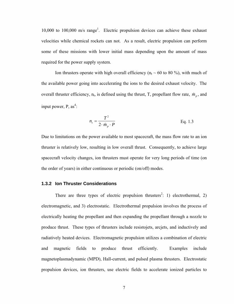
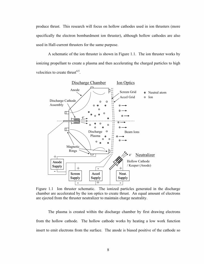
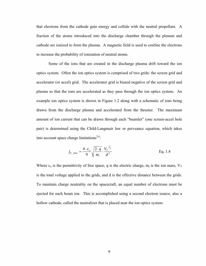

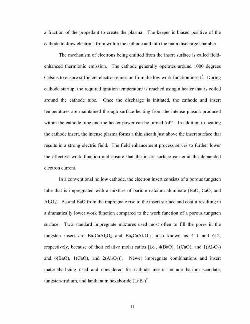


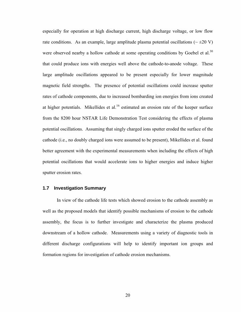


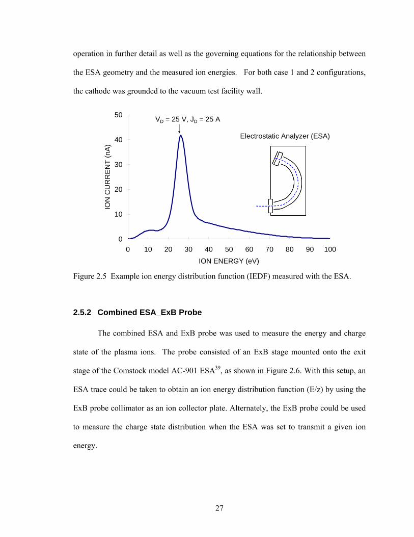
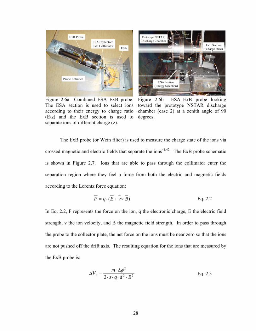

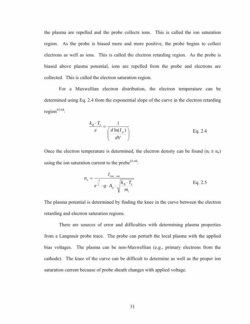
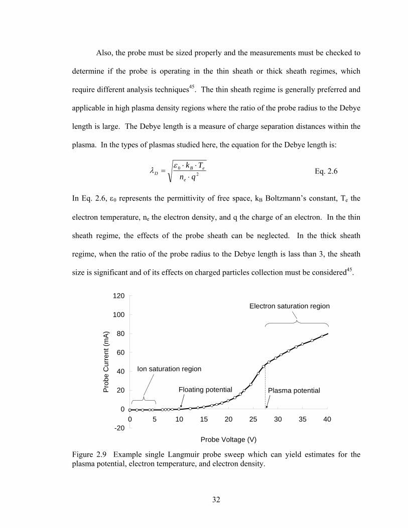

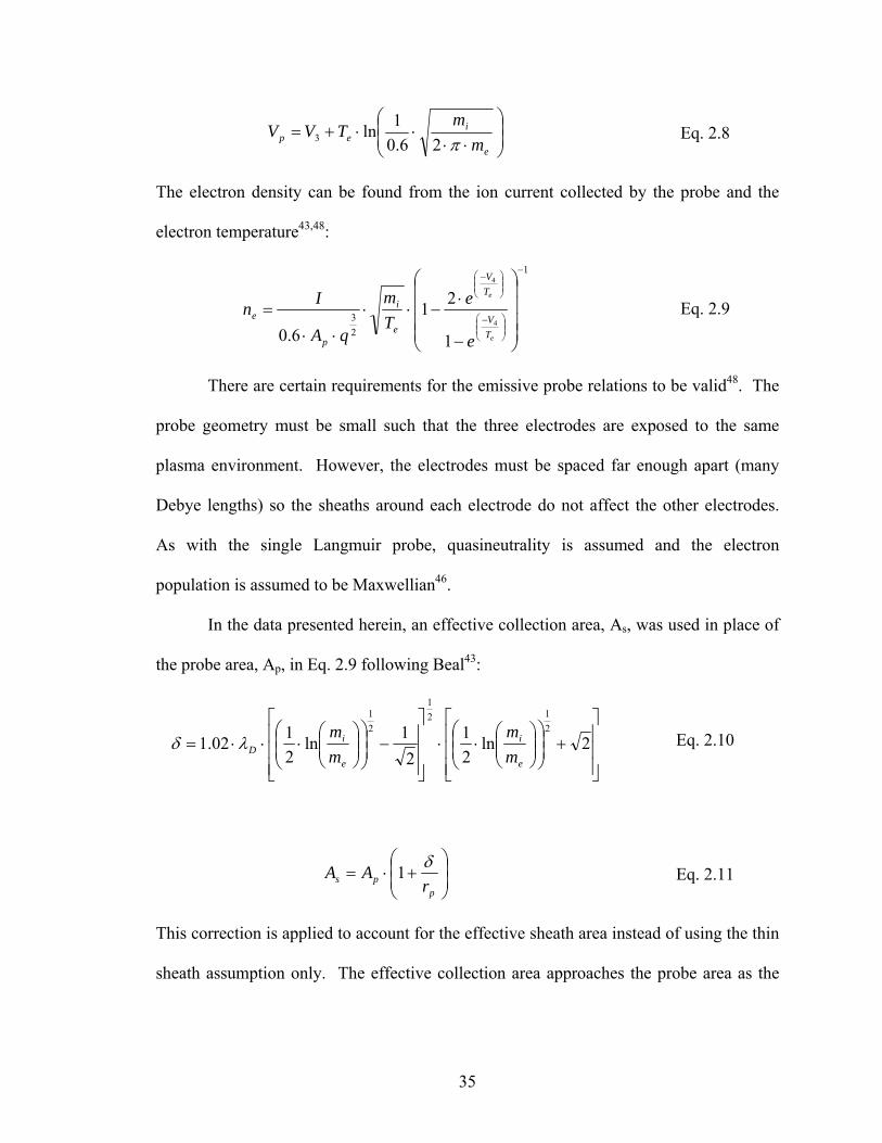


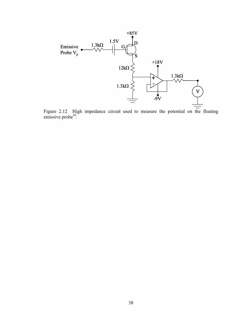

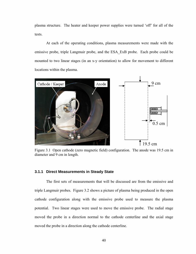
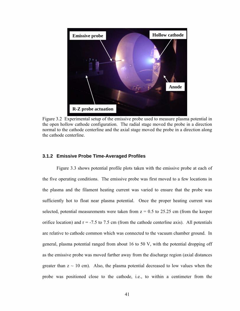

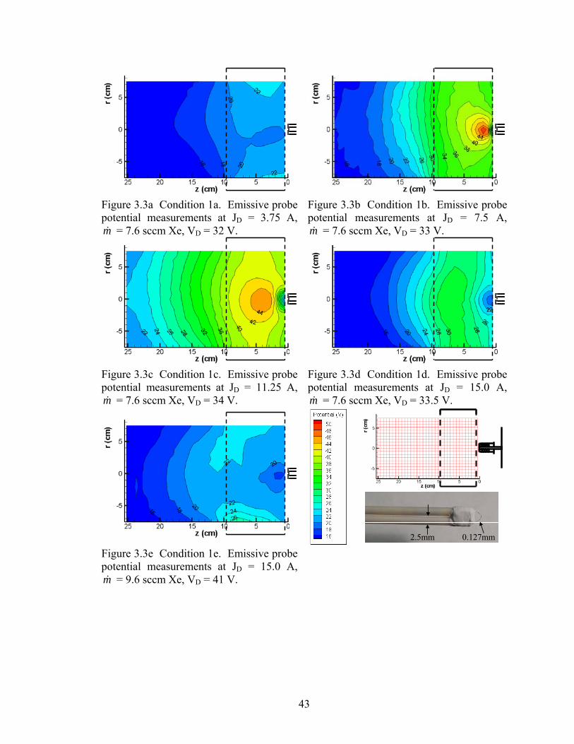
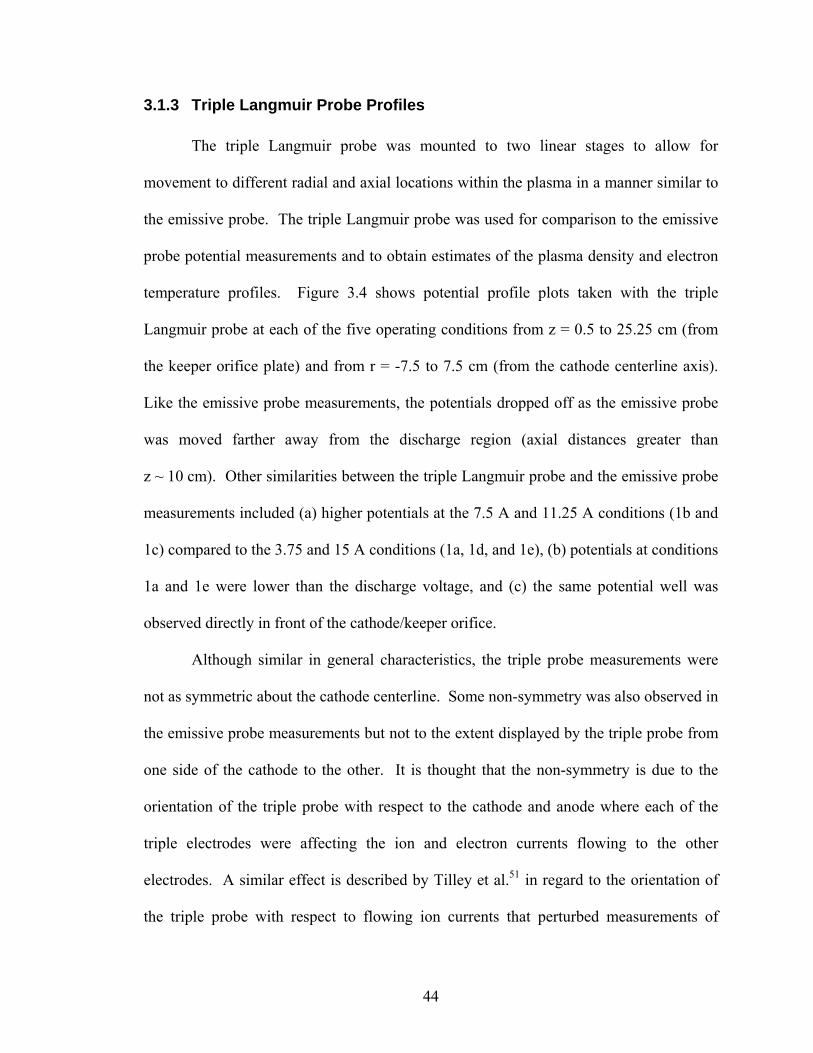


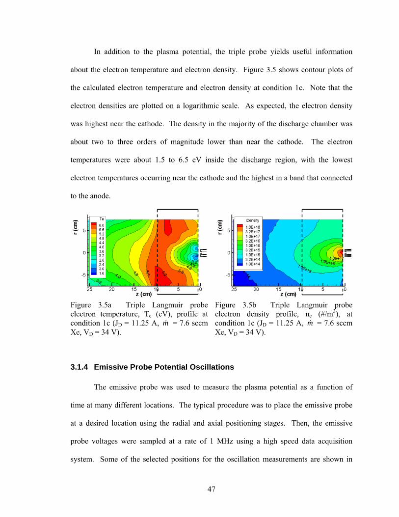

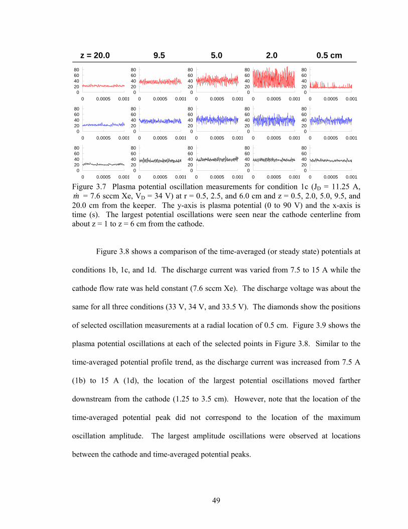
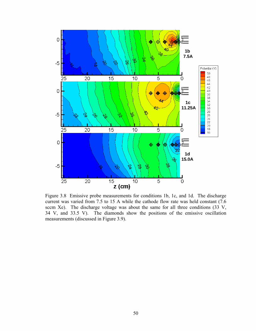


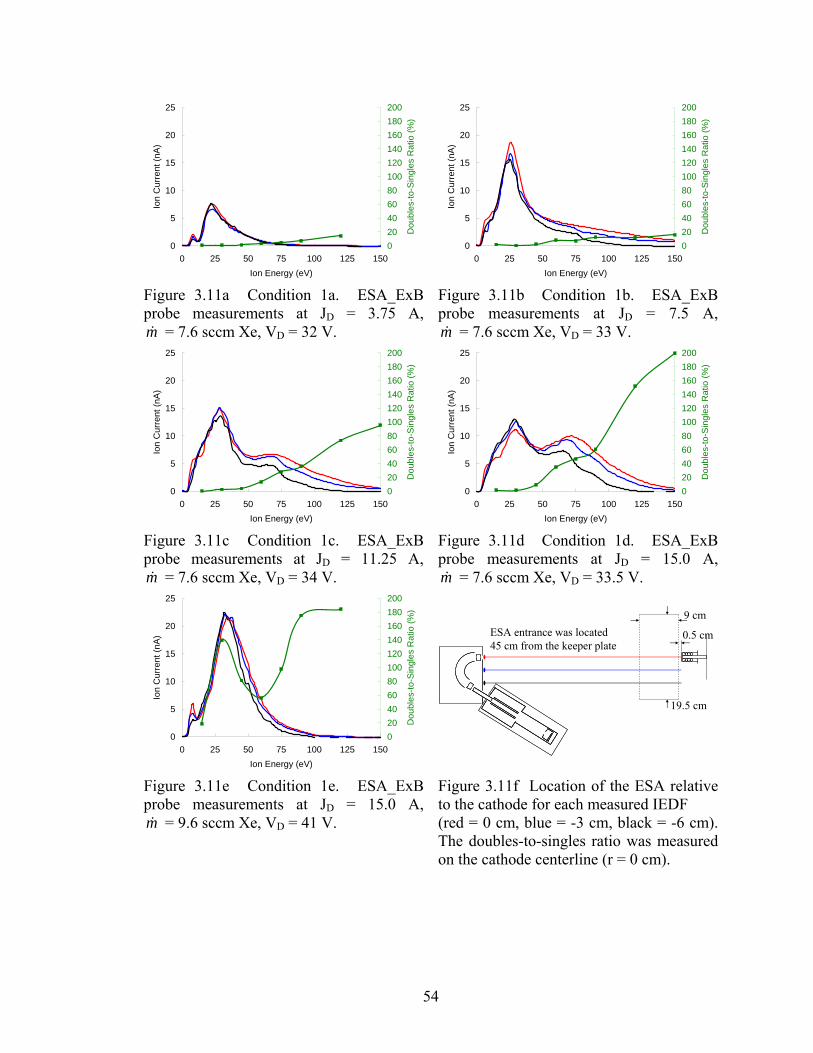


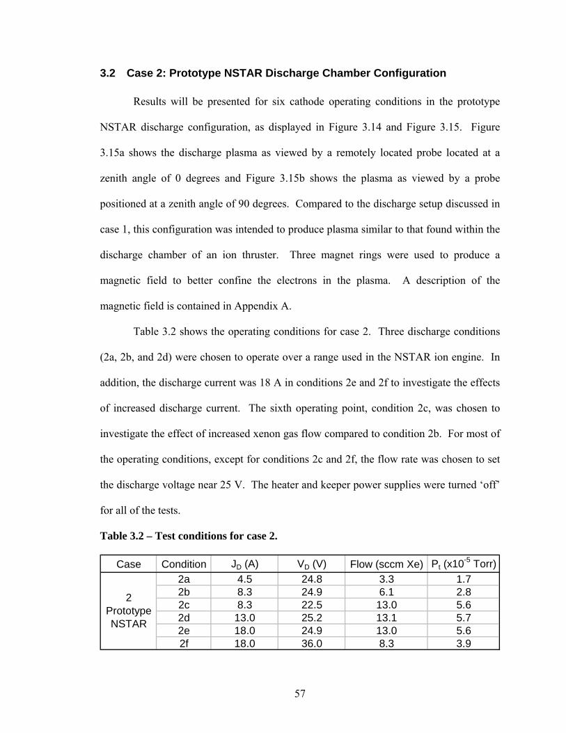
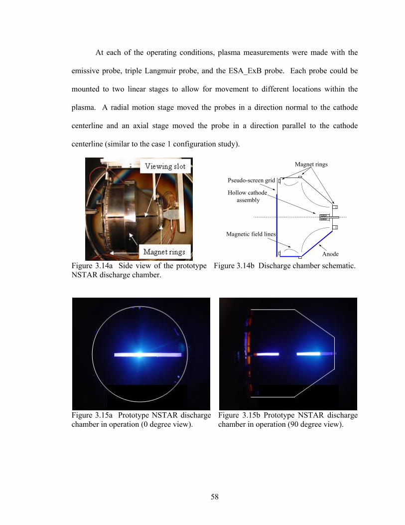

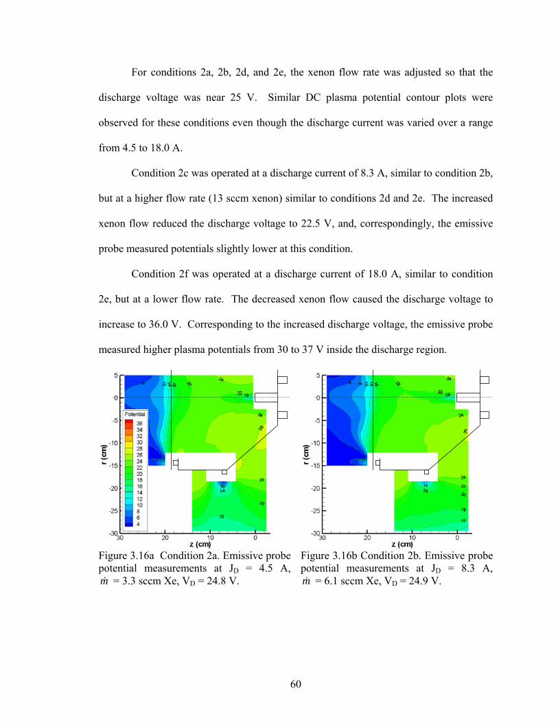


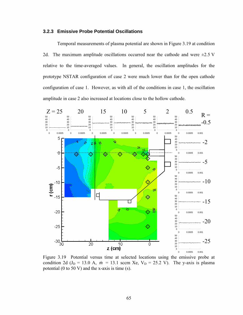

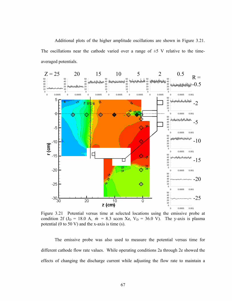


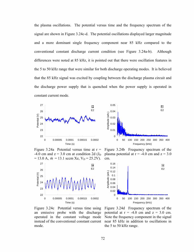

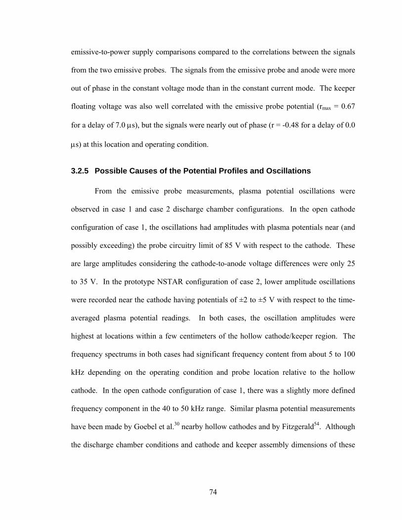
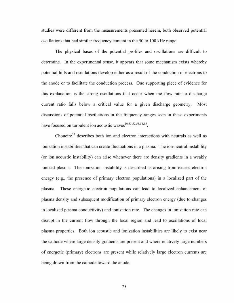
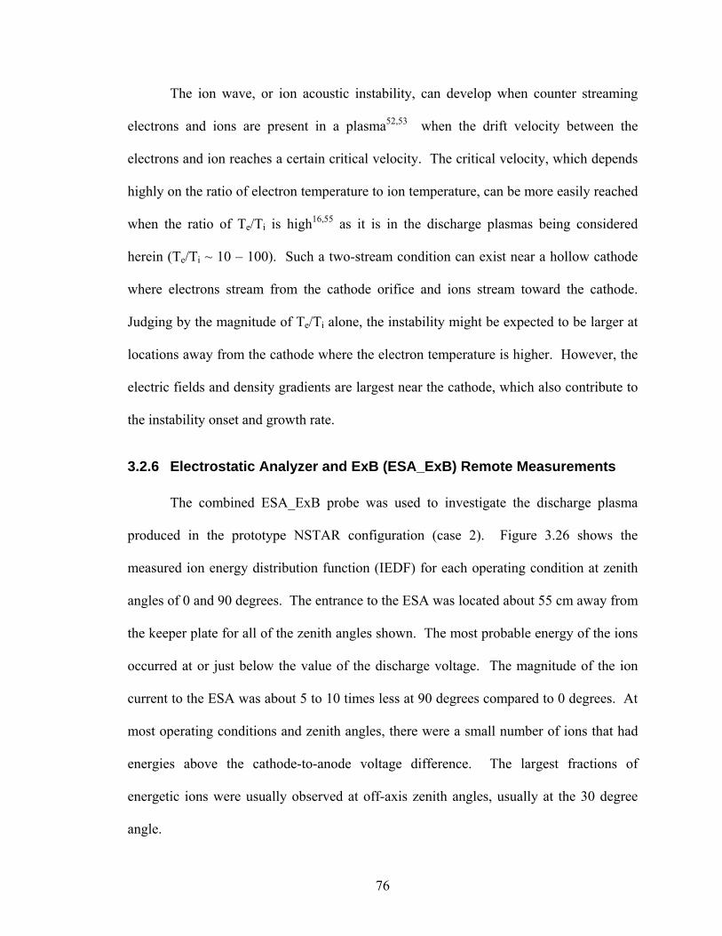


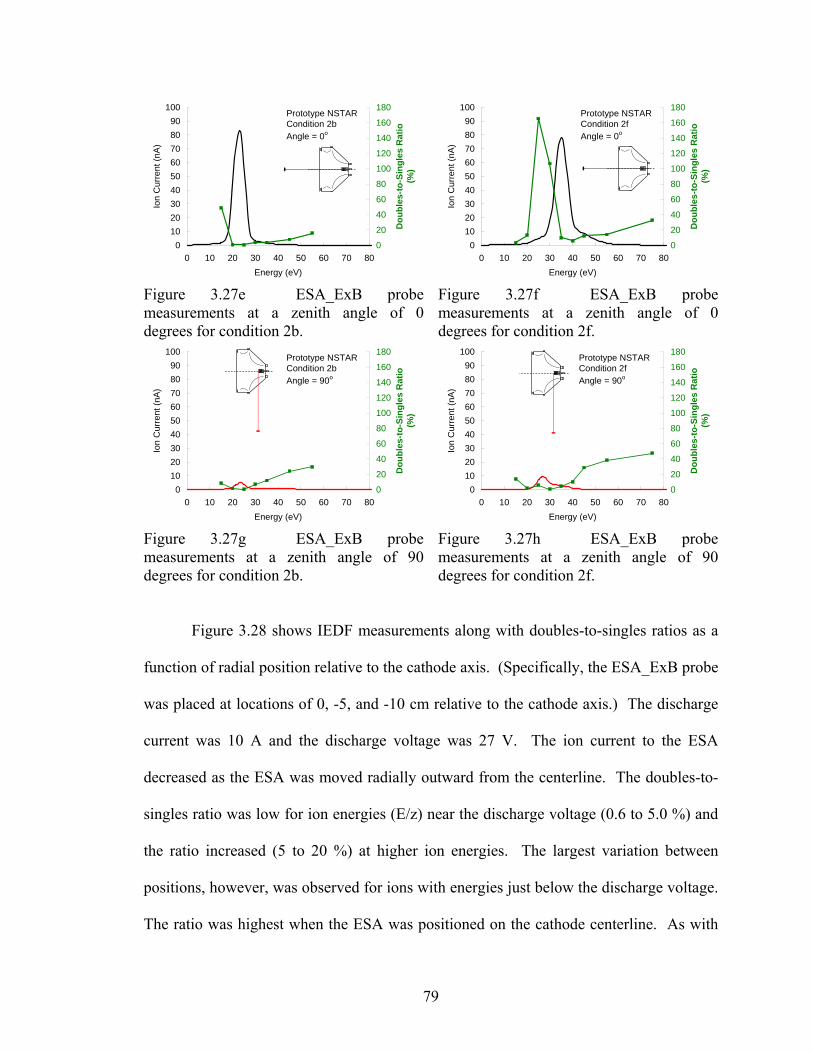
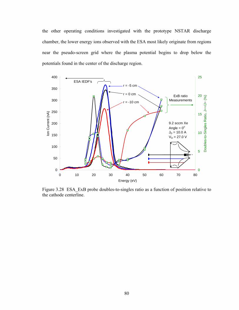

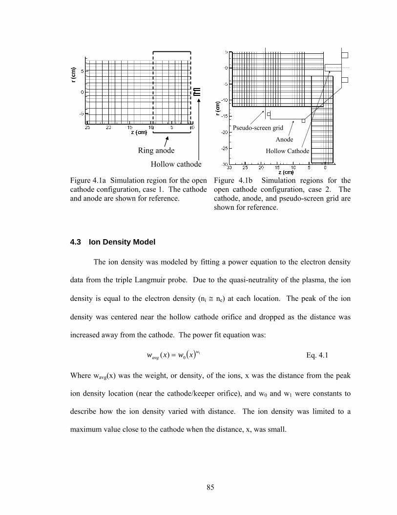


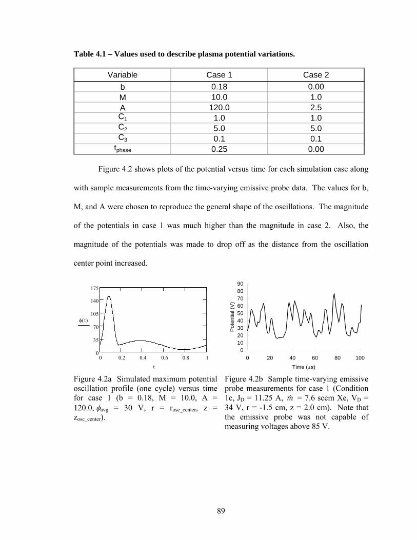
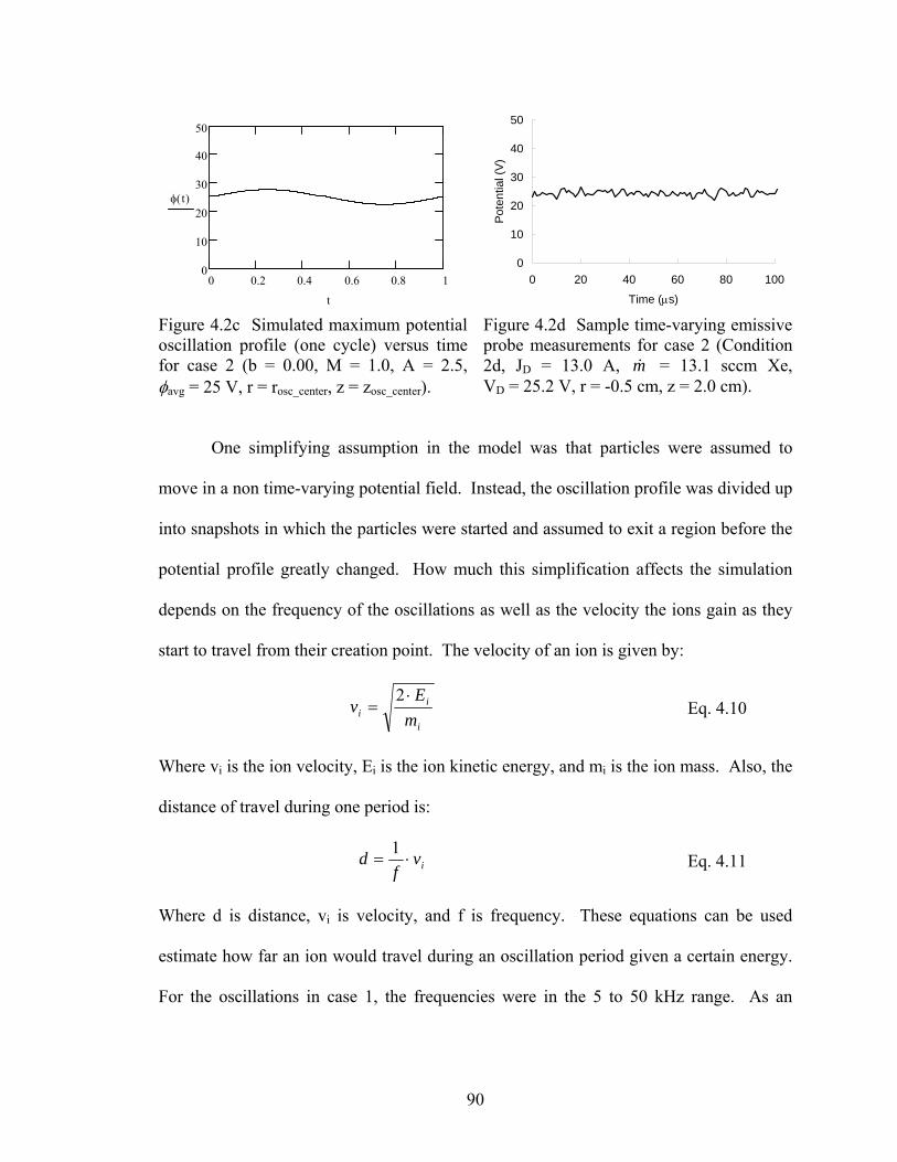
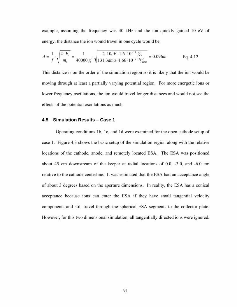
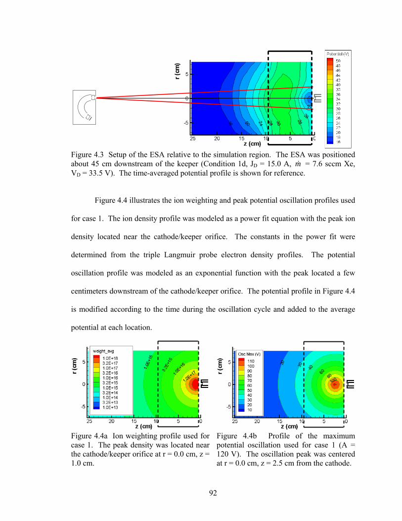


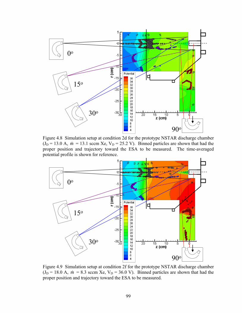
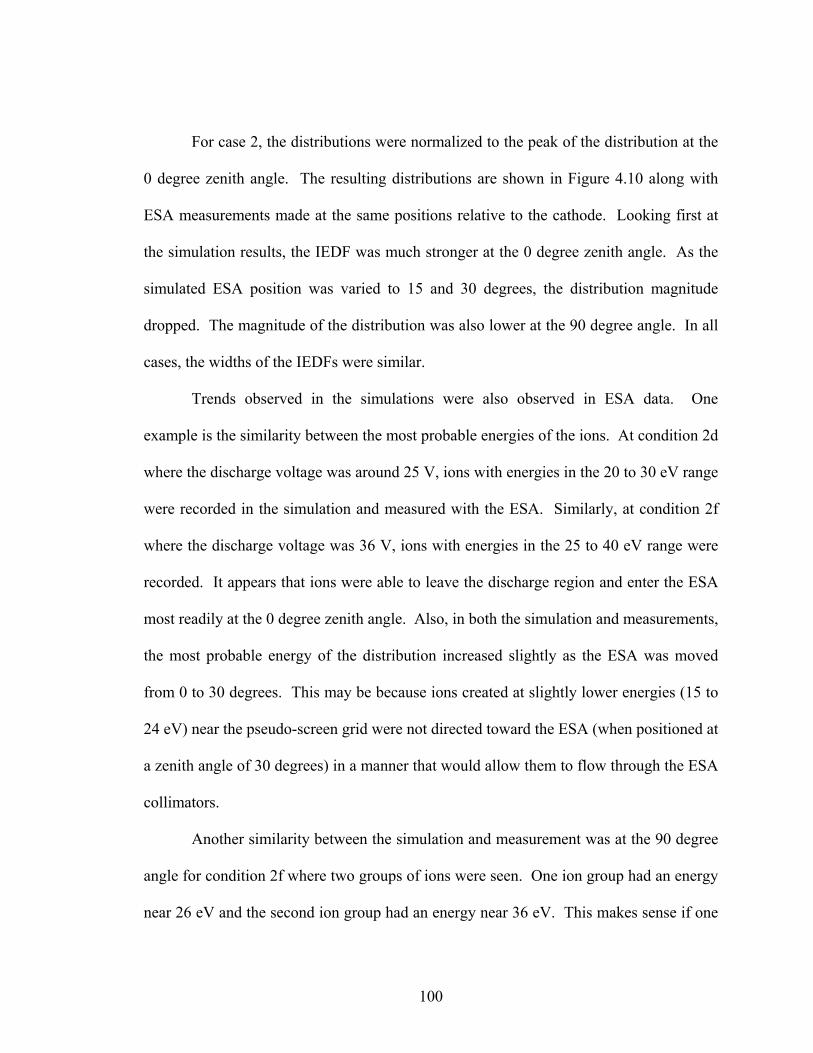
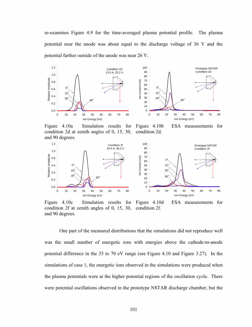


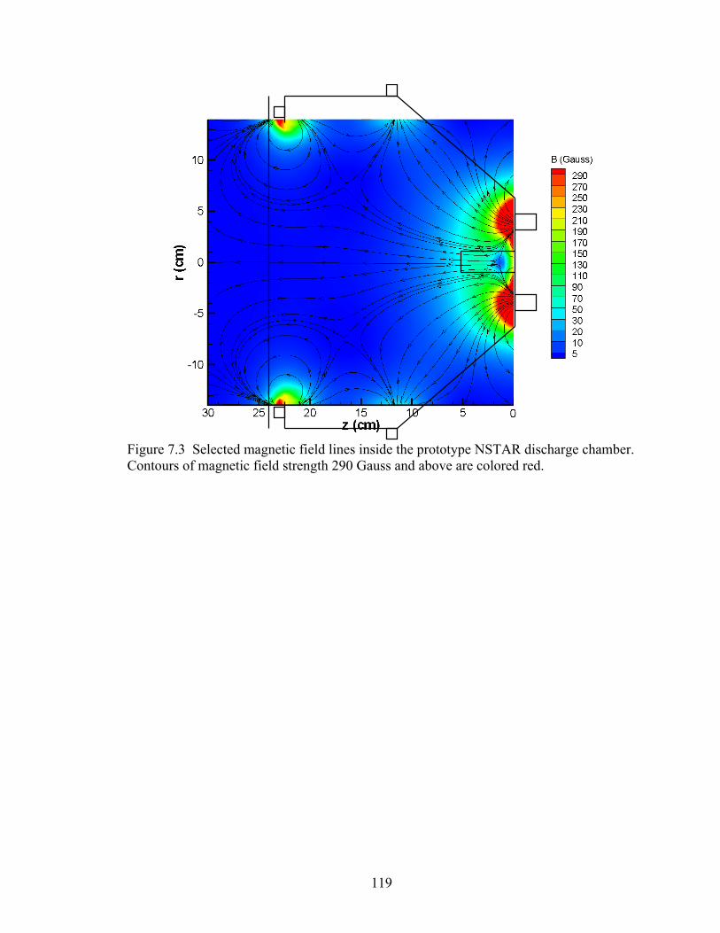


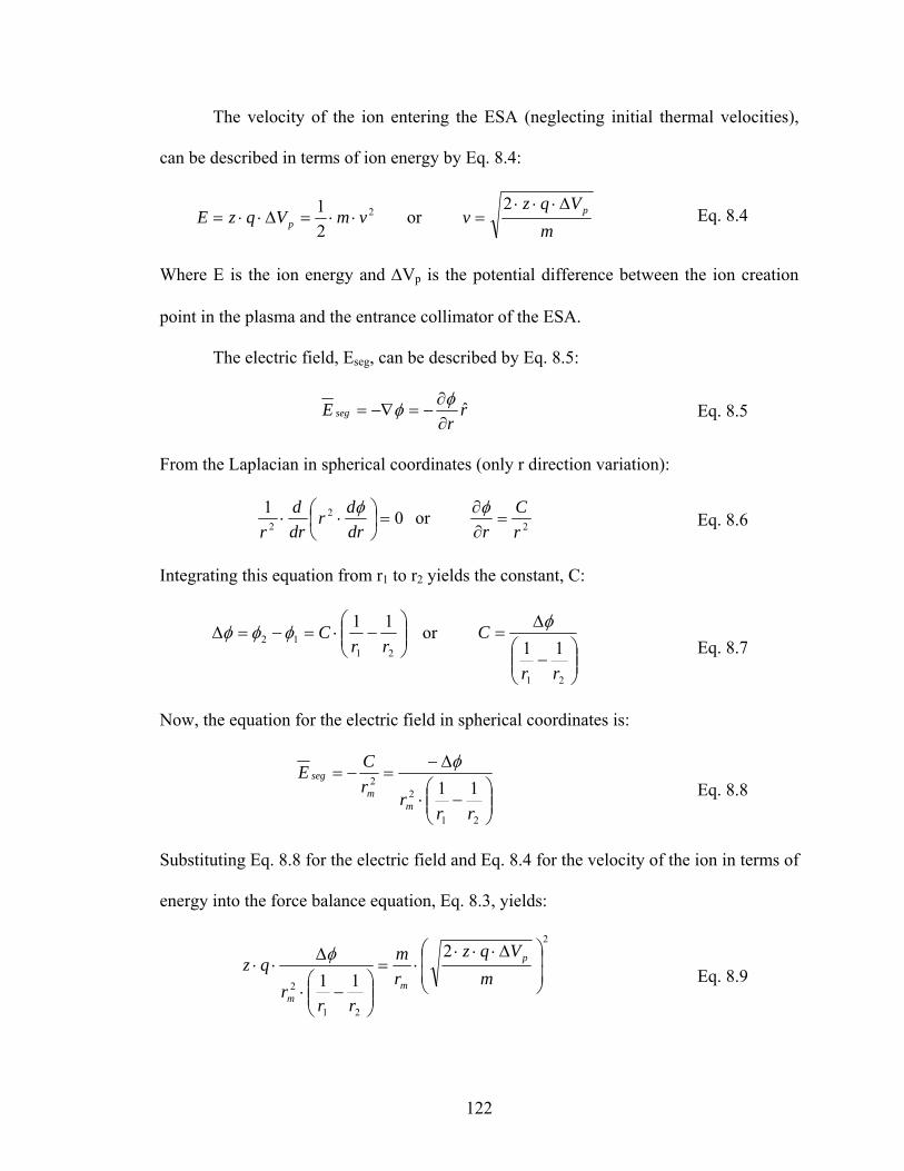


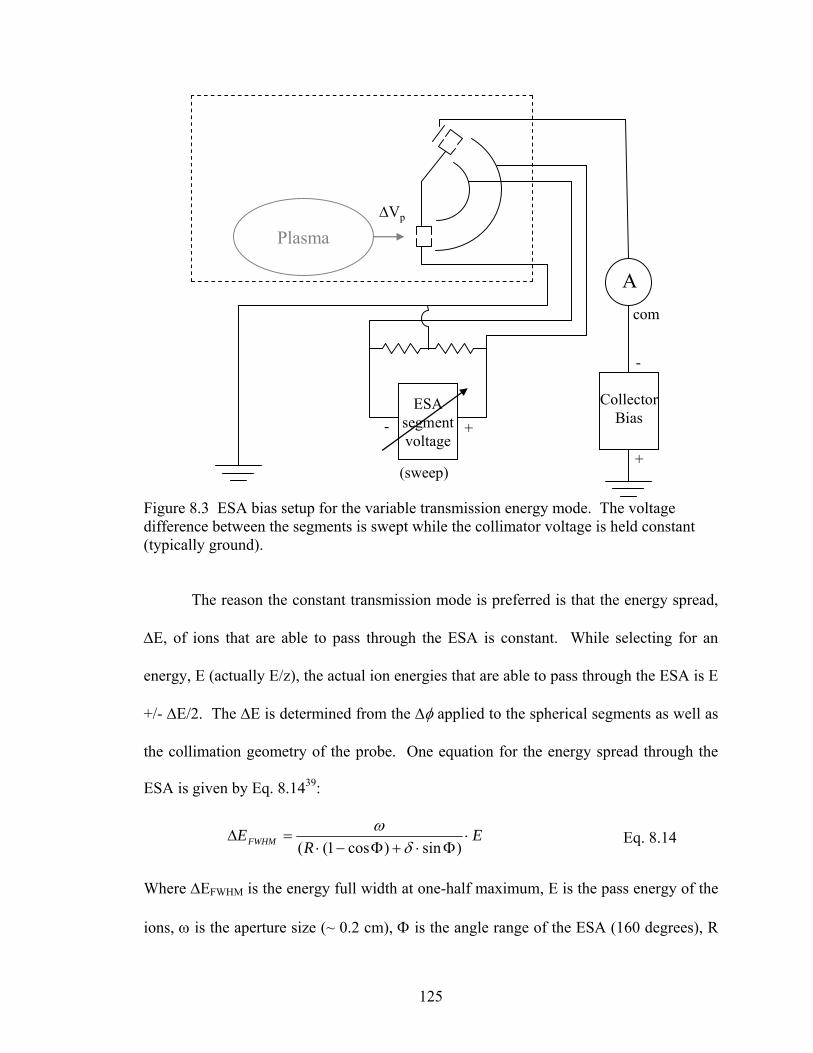
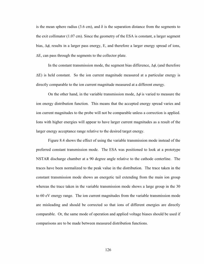
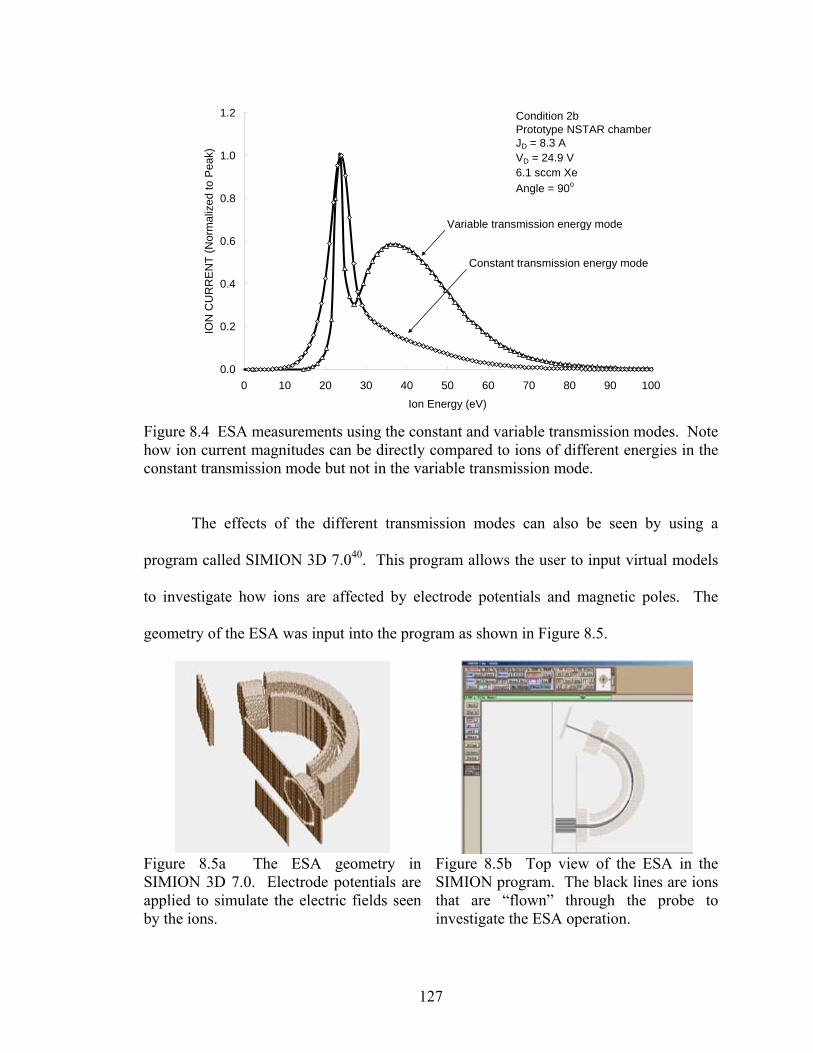

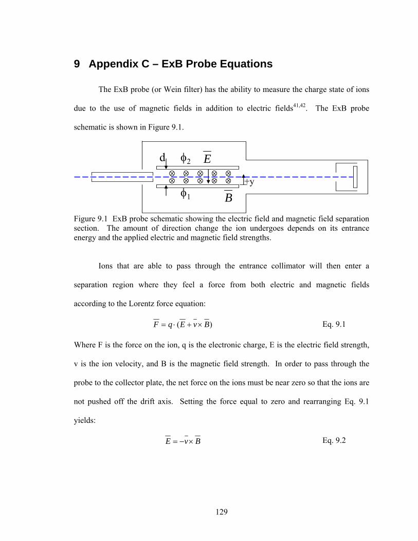


![Princeton Plasma Physics Laboratory · 2008. 3. 4. · ambient plasma with an accelerated ion beam [16]. In the described experiments, we conducted plasma measurements inside the](https://static.documents.pub/doc/80x56/60aa39cfa2904713863d8545/princeton-plasma-physics-laboratory-2008-3-4-ambient-plasma-with-an-accelerated.jpg)


