Dissertation Resource Management in Heterogeneous Computing Systems with Tasks of Varying Importance Submitted by Bhavesh Khemka Department of Electrical and Computer Engineering In partial fulfillment of the requirements For the Degree of Doctor of Philosophy Colorado State University Fort Collins, Colorado Summer 2014 Doctoral Committee: Advisor: Anthony A. Maciejewski Co-Advisor: H. J. Siegel Sudeep Pasricha Gregory A. Koenig Patrick J. Burns
Transcript
Dissertation
Resource Management in Heterogeneous Computing Systems
with Tasks of Varying Importance
Submitted by
Bhavesh Khemka
Department of Electrical and Computer Engineering
In partial fulfillment of the requirements
For the Degree of Doctor of Philosophy
Colorado State University
Fort Collins, Colorado
Summer 2014
Doctoral Committee:
Advisor: Anthony A. MaciejewskiCo-Advisor: H. J. Siegel
Sudeep PasrichaGregory A. KoenigPatrick J. Burns
Copyright by Bhavesh Khemka 2014
All Rights Reserved
Abstract
Resource Management in Heterogeneous Computing Systems
with Tasks of Varying Importance
The problem of efficiently assigning tasks to machines in heterogeneous computing en-
vironments where different tasks can have different levels of importance (or value) to the
computing system is a challenging one. The goal of this work is to study this problem in
a variety of environments. One part of the study considers a computing system and its
corresponding workload based on the expectations for future environments of Department
of Energy and Department of Defense interest. We design heuristics to maximize a perfor-
mance metric created using utility functions. We also create a framework to analyze the
trade-offs between performance and energy consumption. We design techniques to maximize
performance in a dynamic environment that has a constraint on the energy consumption.
Another part of the study explores environments that have uncertainty in the availability of
the compute resources. For this part, we design heuristics and compare their performance
in different types of environments.
ii
Acknowledgements
This dissertation has been made possible by the efforts and support of many people.
First and foremost, I would like to thank my advisors: Dr. Anthony A. Maciejewski and
Dr. Howard J. Siegel for taking the enormous time and energy to impart an abundance of
valuable lessons over countless meetings these past five years. Their knowledge, desire for
perfection, patience, attention to detail, sense of humor, and wisdom have led to an amazing
learning experience. I cannot thank them enough and I will always be grateful to them. I
would also like to thank Dr. Sudeep Pasricha for his guidance and inputs. His constant push
to model real systems as closely as possible has helped shape and direct many parts of the
different research projects. Dr. Gregory A. Koenig, who has been the lead for all the research
projects that were done in collaboration with Oak Ridge National Laboratory (ORNL) and
the U.S. Department of Defense (DoD), has always been a caring and supportive mentor
(including during my internship at ORNL). His readiness to teach and to foster my growth
has been very motivating and I will always be thankful to him for that. I would like to thank
Dr. Patrick Burns for critiquing this work, providing constructive feedback, and for serving
on my committee.
I would like to thank the organizations that funded the different research projects of this
dissertation. Without their support and resources, the research would not have been possible.
Parts of the research in this dissertation were supported by the Colorado State University
George T. Abell Endowment and the National Science Foundation under grant number CNS-
0905339. Parts of the research in this dissertation used resources of the National Center
for Computational Sciences at ORNL, supported by the Extreme Scale Systems Center at
ORNL, which is supported by DoD under subcontract numbers 4000094858 and 4000108022.
iii
Some parts of the research also used the CSU ISTeC Cray System supported by National
Science Foundation under grant number CNS-0923386.
I would like to thank our collaborators at ORNL and DoD: Chris Groer, Marcia Hilton,
Gene Okonski, Steve Poole, Sarah Powers, Jendra Rambharos, and Mike Wright, for their
patience and willingness to have teleconference calls on a weekly basis during the past four
years. Their inputs based on hands-on experience of how schedulers work in the real world
has been invaluable in guiding the research. It truly has been a unique learning experience.
I am thankful to my teammate and friend, Ryan Friese, for the innumerable discussions,
long brainstorming sessions, collaborative writing and code development, laughter, and last
minute favors. It has been an absolute delight to work with him.
My sincere thanks to the members of the robust computing research group at CSU:
Abdulla Al-Qawasmeh, Mohsen Amini, Jonathan Apodaca, Luis D. Briceno, Daniel Dauwe,
Tim Hansen, Eric Jonardi, Paul Maxwell, Mark Oxley, Greg Pfister, Jerry Potter, Jay Smith,
Kyle Tarplee, and Dalton Young, for their insightful and helpful suggestions and feedback
regarding not only the research but also the presentation of the material throughout my
Ph.D.
Many research projects in this dissertation used the CSU ISTeC Cray System for running
the simulation experiments. I would like to extend thanks to the system administrators: Dr.
Richard Casey, Wimroy D’Souza, and Daniel Hamp for their assistance and quick response.
With their help I was able to finish my experiments sooner, and as a result perform more
extensive tests and still get results in a timely manner.
I am deeply indebted to my parents, Mahesh Khemka and Kiran Khemka, for their
undying love and constant support throughout my life. Their care and wisdom are beyond
compare. Even though they were away during my Ph.D., memories of their support and
iv
care kept me going: the nutritious foods in the wee hours of the morning, the many wise
advices, their forward-thinking mentality always looking out for me, and the freedom and
encouragement to let me pursue whatever I want. I am truly blessed to have such wonderful
parents. I also want to thank my extremely caring sisters: Ritu Kedia, Raksha Rajdev, and
Rakhee Divakaran for their perennial support. They have always shown me the humor in
places where I see none.
Priya Naik and Karthik Kadappan have been much more than friends to me in these past
five years. They have been with me through all the lowest lows with their genuine concern
and encouragement and during the highs to celebrate the moment in an ever-more grander
fashion. My heart-felt thanks to them for being patient and understanding with me and for
their heart-warming love and support.
I would like to thank Saket Doshi and Gaurav Madiwale for all the help, for always being
there, for so many fun memories, and for just being the great people they are. I am also
very thankful for all the amazing friends at the Indian Students Association at CSU. My
experience here would be incomplete and not as lively without them.
In closing, I would like to thank my Guru who has made everything possible, including
this wonderful experience to learn and to grow. I cannot thank him enough for his guidance,
blessings, patience, encouragement, love, and support.
This dissertation is typset in LATEX using a document class designed by Leif Anderson.
v
DEDICATION
To the most nurturing and enlightened parents that ever lived
High-performance computing (HPC), high-throughput computing, and many-task com-
puting are currently used to solve a host of problems. These environments may be heteroge-
neous and oversubscribed. By heterogeneous we mean that different tasks may have varied
execution times on the different machines. By oversubscribed we mean that the workload
of tasks is large enough such that the total offered work exceeds the capacity of the sys-
tem in steady state operation (or over an extended period). The process of allocating tasks
to machines for execution is often referred to in the literature as “resource allocation” or
“mapping,” and the process of ordering the tasks’ execution is referred to as “scheduling.”
The mapping and scheduling problem has been known, in general, to be NP-Complete [1],
and therefore heuristics are commonly used to find a solution to this problem. Performing
resource management in oversubscribed heterogeneous environments further complicates the
problem.
In many scenarios, different tasks are of different “importance” to the enterprise com-
puting system. In such environments, it becomes beneficial to account for the differences
in the values of different tasks to make resource allocation decisions. This is particularly
important in oversubscribed heterogeneous computing environments. In this dissertation, we
design and analyze techniques to perform mapping and scheduling decisions in computing
environments that have tasks with different “reward” or “utility” values.
In Chapter 2, we design utility functions to create a performance metric for schedulers
in a dynamic oversubscribed heterogeneous computing environment. We model a computing
system and its intended workload based on the expectations for future environments of
1
Department of Energy and Department of Defense interest. We design twelve heuristics and
compare their performance. We also create additional operations to assist the heuristics in
making mapping decisions. We analyze the performance of the heuristics under two different
levels of oversubscription.
During 2010, global HPC systems accounted for 1.5% of total electricity use, while in
the U.S., HPC systems accounted for 2.2% [2]. With the rising demand and costs of energy
it becomes extremely important to make scheduling decisions in an energy-efficient manner.
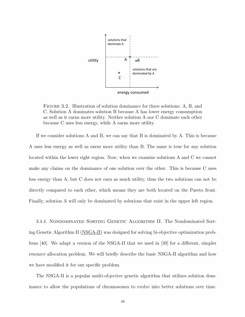
Chapter 3 explores the bi-objective problem of maximizing performance and minimizing
energy consumption. The goal is to create a Pareto front of solutions from which the system
administrator can pick a point to operate by analyzing the trade-offs between performance
and energy consumption. Chapter 4 deals with energy-constrained utility maximization. We
design an energy filtering technique that helps heuristics avoid mapping decisions that can
lead to high energy consumption. Possible extensions for both of these works are mentioned
in Chapter 6.
In many large-scale distributed computing environments, it is common for failures to
randomly occur in the compute resources. These effects are estimated to worsen as we
approach exa-scale. Making resource allocation decisions while being aware of such failures
further complicates the scheduling problem. In Chapter 5, we explore this problem by
studying and comparing the performance of different heuristics in a variety of environments.
Directions for future work of this study are detailed in Chapter 6.
2
CHAPTER 2
Utility Functions and Resource Management1
2.1. Introduction
A utility function for a task describes the value of completing the execution of the task at
a specific time [5–9]. Utility functions capture the time-varying importance of a task to both
the user and the enterprise as a whole. In this work, the value of completing a task decays
over time and so we model monotonically-decreasing utility functions. The design of utility
functions needs to be flexible to capture the importance of tasks within a diverse user base.
In practice, utility functions may be created through a collaboration between the user and
the owner of the computing system. We design dynamic resource management techniques
to maximize the total utility that can be earned by completing tasks in an oversubscribed
heterogeneous distributed environment. By oversubscribed we mean that the workload is
large enough that the total desired work exceeds the capacity of the system in steady state
operation, i.e., over an extended period. By a heterogeneous environment we mean that the
execution time of each task may vary across the suite of machines. We model this computing
environment and the workload of tasks that arrive dynamically. A scheduler makes resource
allocation decisions to map (assign) the incoming tasks to the machines. The total utility
earned from all completed tasks captures how much useful work was done and how timely
that information was to the user. The system characteristics and the workload parameters are
based on environments being investigated by the Extreme Scale Systems Center (ESSC) at
1This work was done jointly with the Ph.D. students Luis D. Briceno and Ryan Friese. The full list ofco-authors is at [3]. A preliminary version of portions of the work mentioned in this chapter appeared in[4]. This research used resources of the National Center for Computational Sciences at Oak Ridge NationalLaboratory, supported by the Extreme Scale Systems Center at ORNL, which is supported by the Departmentof Defense under subcontract numbers 4000094858 and 4000108022. This research also used the CSU ISTeCCray System supported by NSF Grant CNS-0923386.
3
Oak Ridge National Laboratory (ORNL). The ESSC is part of a collaborative effort between
the Department of Energy (DOE) and the Department of Defense (DoD) to perform research
and deliver tools, software, and technologies that can be integrated, deployed, and used in
both DOE and DoD environments.
We design a method that can be used to create utility functions by defining three pa-
rameters: priority, urgency, and utility class. The priority of a task represents the level of
importance of a task to the enterprise, while urgency indicates how quickly the task loses
utility. The utility class provides finer control of the shape of the utility function by parti-
tioning it into intervals. We assume that the scheduler has experiential information about
the execution time of each type of task on each type of machine. However, the scheduler
does not know the arrival time, utility function, or type of each task until the task arrives.
We use two forms of dynamic heuristics to perform the resource allocation decisions.
Immediate-mode heuristics schedule only the incoming task and do not have the opportunity
to re-map tasks that are already in machine queues (e.g., [10–12]). Batch-mode heuristics
consider a set of tasks and have the ability to re-map tasks that are enqueued and waiting
to execute (e.g., [10, 11]). We create seven immediate-mode and five batch-mode heuristics,
and analyze their performance using simulation experiments. To examine the effect of over-
subscription on the performance of the heuristics, we simulate two levels of oversubscription.
We also study the effect of heuristic variations, such as dropping tasks and altering the
mapping decision frequency for the batch-scheduler.
The contributions of this chapter are: (a) a model of the planned DOE/DoD oversub-
scribed heterogeneous high performance computing environment, (b) the design of a metric
using utility functions, based on the three parameters of priority, urgency, and utility class,
to measure the performance of schedulers in an oversubscribed heterogeneous computing
4
environment, (c) the design of twelve heuristics to perform the scheduling operations and
their evaluation over a variety of environments, and (d) the exploration and the analysis of
heuristic variations, such as dropping tasks and varying the number of tasks scheduled at
each batch-mode mapping event.
The remainder of the chapter is organized as follows. In Sec. 2.2, we explain our system
model, including our method to design the utility functions (from the three parameters men-
tioned before), the characteristics of the workload, and the characteristics of the computing
environment. We formally give our problem statement in Sec. 2.3, and introduce our metric
to compare the performance of resource allocation heuristics. In Sec. 2.4, we describe the
various heuristics we have designed and the method to drop tasks. We compare our study
to other work from the literature in Sec. 2.5. We explore the design of our simulation ex-
periments in Sec. 2.6. In Sec. 2.7, we present and analyze our simulation results. Finally,
we conclude the chapter and discuss possible future directions in Sec. 2.8.
2.2. System Model
2.2.1. Utility Functions.
2.2.1.1. Overview. In our study, it is assumed that an enterprise computing system earns
a certain amount of utility for completing each task. The amount of utility earned depends
on the task and the time at which the task was completed relative to the time it arrived,
and reflects its importance to the system. We use utility functions to model the time-
varying benefit of completing the execution of a task. The utility functions we model are
monotonically decreasing. This implies that if a task takes longer to complete, it cannot earn
higher utility. We understand that there may be use cases for non-monotonically-decreasing
utility functions, but they are not considered here. We design a flexible utility function for a
5
task that is defined by three parameters: priority, urgency, and utility class. The goal is to
use a small set of parameters that the users understand and enables the users to obtain the
desired utility curve. By using a combination of these parameters we can create a variety of
shapes for the utility functions. These parameters were designed based on the needs of the
ESSC at ORNL. We expect that these parameters will be set by the customer (submitting the
job) in collaboration with the system owner and the overall system administration policies.
2.2.1.2. Parameters.
Priority. Priority represents the importance of the task to the organization. It sets the
maximum value of a utility function. As the functions are monotonically decreasing, this is
equivalent to the starting value of the utility function. Let π(p) be the maximum utility of
tasks belonging to priority level p, where p ∈ critical, high,medium, low. Each of these
priority levels has a fixed value of maximum utility associated with it. Fig. 2.1a shows
utility functions with different levels of priority for a fixed level of urgency (defined below).
As shown in Fig. 2.1a, a task’s utility does not begin to decay as soon as it arrives, because
this would make the maximum utility value of a task unachievable (i.e., the task needs
non-zero time to execute). In Sec. 2.6.2, we describe how we determine the length of this
interval.
Urgency. The urgency of a task models the rate of decay of the utility of that task over
time. It affects the “shape” of the utility function. Tasks that are more urgent will have their
utility values decrease at a faster rate than less urgent tasks. In this study, we model the
decay of utilities as an exponential (other functions may be used). Let ρ(r) be the exponential
decay rate of tasks belonging to urgency level r, where r ∈ extreme, high,medium, low.
Fig. 2.1b illustrates utility functions with different urgency levels for a fixed priority level.
6
The urgency level of a task along with the task’s average execution time control the duration
for which the starting utility value of a task does not decay (see Sec. 2.6.2).
Utility Class. A utility class is used to fine-tune a utility function by dividing the function
into a set of intervals with discrete characteristics. We define each interval (except the first)
to have three parameters: a start time, a percentage of maximum utility at that start time,
and an exponential decay rate modifier. By defining different utility classes we can devise a
wide variety of utility functions. We could set a hard deadline for a task by having the utility
of the task drop to zero. For our simulations, we created four utility classes and each task
belongs to one of these four classes (the number of utility classes can be domain dependent).
The first element within a utility class is the set of time intervals that partition the time
axis of the utility function (except the end time of the first interval). Let t(k, c) be the start
time of the kth interval relative to the arrival time of a task belonging to utility class c.
The second element in a utility class sets the percentage of the maximum utility at the
start of each of the intervals except the first. Let ψ(k, c) be this percentage for the kth
interval, where 0 ≤ ψ(k, c) ≤ 1 and ψ(k, c) ≤ ψ(k− 1, c) for k > 1. Therefore, the maximum
utility value in the kth interval of a utility function for a task with a priority level p and
utility class c is given by, Ψ(k, c, p) = ψ(k, c)× π(p).
The final element in a utility class c is a modifier, δ(k, c), to the exponential decay rate
of the interval k, with k > 1 to ignore the first interval. The exponential decay rate in
interval k of a utility function with urgency level r and utility class c is given by, ∆(k, c, r) =
δ(k, c) × ρ(r). The values of this modifier are typically near 1, because the purpose of this
modifier is to provide small differences in the decay rate across the intervals.
7
0!1!2!3!4!5!6!7!8!9!
τ+0! τ+10! τ+20! τ+30! τ+40! τ+50!
utili
ty !
completion time from arrival!
for a fixed urgency level!
(a)
0!
1!
2!
3!
4!
5!
τ+0! τ+10! τ+20! τ+30! τ+40! τ+50!
utili
ty !
completion time from arrival!
for a fixed priority level!
(b)
Figure 2.1. (a) Four utility functions with different priority levels and afixed urgency level showing the decay in utility for a task after its arrival timeτ . The curves labeled “c,” “h,” “m,” and “l” are the curves with critical,high, medium, and low priorities, respectively. (b) Four utility functions withdifferent urgency levels and a fixed priority level showing the decay in utilityfor a task after its arrival time τ . The curves labeled “e,” “h,” “m,” and “l” arethe curves with extreme, high, medium, and low urgency levels, respectively.The length of time for which the starting utility value of a task persists (doesnot decay) is shorter for more urgent tasks.
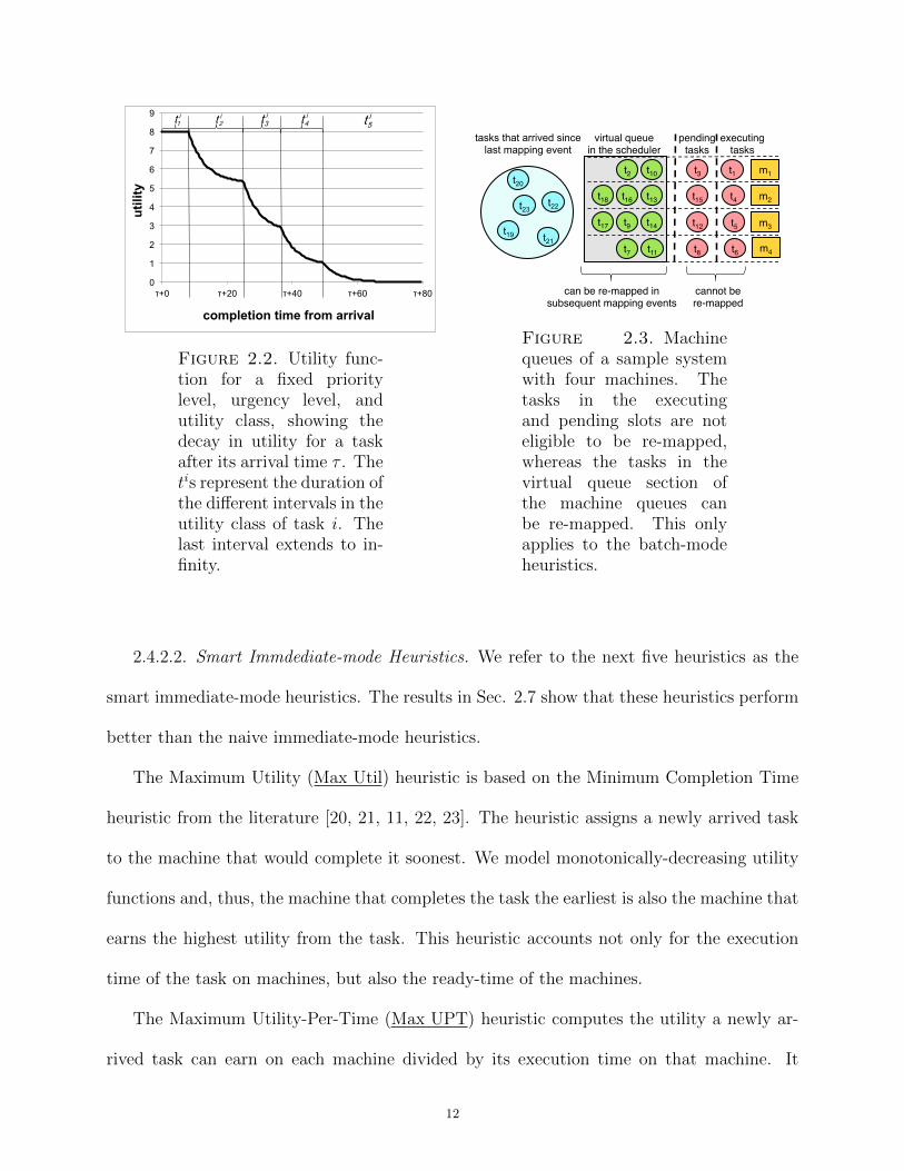
Fig. 2.2 shows a utility function (at a fixed priority and urgency level) partitioned into
separate intervals, each with its own rate of decay and starting utility value. The last interval
shows that the utility drops to zero as time tends to infinity.
2.2.1.3. Construction of a Utility Function. Let p be the priority level, r the urgency
level, and c the utility class of a task i. The utility value U(p, r, c, t) at any time t relative to
the arrival time of the task, where t(k, c) ≤ t < t(k+1, c), is given by the following equation:
2.2.2. Model of Environment. We group tasks with similar computational require-
ments into task types and machines with similar performance capabilities into machine types.
We model a heterogeneous environment, where the execution times of different task types
may vary across the different machine types. We assume we are given an Estimated Time to
8
Compute (ETC) matrix, where ETC(i, j) is the estimated time to compute a task of type i
on a machine of type j. This is a common assumption in the resource management literature
[13–18]. For simulation purposes, we use a synthetic workload as described in Sec. 2.6.3,
but in practice, one could use historical data to obtain such information [15, 17]. We model
special-purpose and general-purpose machines. The special-purpose machine types have the
ability to execute certain task types much faster than the general-purpose machine types,
but may be incapable of executing other task types. Further details are in Sec. 2.6.3.
We model a dynamic environment where tasks arrive throughout a 24 hour period. The
scheduler does not know the arrival time, utility function, or type of each task until the
task arrives. The system is composed of dedicated compute resources with a workload large
enough to create an oversubscribed environment. We assume that the tasks in the workload
are independent (no inter-task communication is required) and serial (each task executes on
a single machine). For scheduling purposes we do not consider the pre-emption of tasks. We
do, however, allow tasks to be dropped prior to execution (see Sec. 2.4.4).
2.3. Problem Statement
Our goal is to design resource management techniques to maximize the overall system
utility achieved in an oversubscribed heterogeneous environment. To solve this problem, we
devise twelve heuristics to perform the scheduling operations and design a metric using utility
functions to measure the performance of schedulers. Once a task arrives, we can calculate
the completion time of the task based on the resource to which it is mapped. Using the
completion time of task i, denoted tcompletion(i), and the task’s utility function parameters
(namely, p(i), r(i), and c(i)), the utility earned by the task can be calculated using Equation
1 to obtain U(p(i), r(i), c(i), tcompletion(i)). Let Ω(tend) be the set of tasks that have completed
9
execution by time tend. The goal of our resource management procedures is to maximize the
total utility that can be earned by the system over the 24 hour period and is computed using:
(2) Usystem(tend) =∑
i∈Ω(tend)
U(p(i), r(i), c(i), tcompletion(i)).
2.4. Resource Management Policies
2.4.1. Overview. The scheduling problem, in general, has been shown to be NP-complete
[1], and therefore it is common to use heuristics to solve this problem. Any time when a
decision has to be made to assign a task to a machine we call a mapping event. The two
types of dynamic heuristics (also known as online heuristics [19]) we use, immediate-mode
heuristics and batch-mode heuristics, differ in the method that a mapping event is triggered
and in the set of tasks that can be scheduled during a mapping event.
In immediate-mode heuristics, a mapping event occurs when a task arrives. The only
exception to this is when the execution of the previous mapping event has not finished before
the arrival of the next task. In that case, the trigger time for the next mapping event is
delayed until the previous mapping event finishes execution. The immediate-mode heuristics
assign the new task to some machine queue. Once the task is put in the machine queue it
cannot be remapped. We design and evaluate seven immediate-mode heuristics.
In batch-mode heuristics, typically mapping events are triggered after fixed time intervals
or a fixed number of task arrivals. If the previous mapping event has not completed execution,
the trigger time of the next mapping event is delayed until the previous mapping event
finishes execution. We refer to the task that is next in-line for execution on a machine queue
as a pending task. We refer to the part of the machine queues that do not include the
executing and the pending tasks as the virtual queues of the scheduler. Fig. 2.3 shows tasks
10
waiting in the virtual queues of an example system with four machines. The batch-mode
heuristics make mapping decisions for both the tasks that have arrived since the last mapping
event and the tasks that are waiting in the virtual queues. This set of tasks is the called
the mappable tasks. The batch-mode heuristics (unlike immediate-mode heuristics) have
the capability to re-map tasks in the virtual queues of scheduler. The batch-mode heuristics
do not re-map pending tasks so the machine does not become idle when its executing task
completes. The simulation results in Sec. 2.7 show that the batch-mode heuristics have a
significant advantage because they have more information available while making a mapping
decision (as they consider a set of tasks). Furthermore they can alter those decisions in the
future by remapping tasks when additional information becomes available. We design and
evaluate five batch-mode heuristics.
2.4.2. Immediate-mode Heuristics.
2.4.2.1. Naive Immediate-mode Heuristics. The first two immediate-mode heuristics do
not consider the execution time estimates of different task types on machine types, nor the
ready-times of the machines (the times that the machines finish execution of their already
queued tasks). These heuristics are used as baseline heuristics for comparison purposes. We
refer to these heuristics as the naive immediate-mode heuristics.
The Random heuristic assigns the newly arrived task to a random machine on which it
can execute (i.e., not a special-purpose machine where it cannot execute). The Round-Robin
heuristic assigns the incoming tasks in a round-robin fashion. The machines are listed in a
randomized order and this ordering is kept fixed. The first task that arrives for a mapping
event is assigned to the first machine (on which it can execute), the next incoming task is
assigned to the next machine (on which it can execute), and so on.
11
0
1
2
3
4
5
6
7
8
9
τ+0 τ+20 τ+40 τ+60 τ+80
utili
ty
completion time from arrival
i1t i
2ti3t i
4t i5t
Figure 2.2. Utility func-tion for a fixed prioritylevel, urgency level, andutility class, showing thedecay in utility for a taskafter its arrival time τ . Thetis represent the duration ofthe different intervals in theutility class of task i. Thelast interval extends to in-finity.
m1!
m2!
m3!
m4!
executing!tasks!
pending tasks!
virtual queue!in the scheduler!
t1!
t4!
t5!
t6!
t3!t2!
t7! t8!
t10!
t13!
t14!
t11!
t16!
t9! t12!
t18!
t17!
can be re-mapped in subsequent mapping events!
cannot be re-mapped!
tasks that arrived since last mapping event
t20
t23
t21 t19
t22 t15!
Figure 2.3. Machinequeues of a sample systemwith four machines. Thetasks in the executingand pending slots are noteligible to be re-mapped,whereas the tasks in thevirtual queue section ofthe machine queues canbe re-mapped. This onlyapplies to the batch-modeheuristics.
2.4.2.2. Smart Immdediate-mode Heuristics. We refer to the next five heuristics as the
smart immediate-mode heuristics. The results in Sec. 2.7 show that these heuristics perform
better than the naive immediate-mode heuristics.
The Maximum Utility (Max Util) heuristic is based on the Minimum Completion Time
heuristic from the literature [20, 21, 11, 22, 23]. The heuristic assigns a newly arrived task
to the machine that would complete it soonest. We model monotonically-decreasing utility
functions and, thus, the machine that completes the task the earliest is also the machine that
earns the highest utility from the task. This heuristic accounts not only for the execution
time of the task on machines, but also the ready-time of the machines.
The Maximum Utility-Per-Time (Max UPT) heuristic computes the utility a newly ar-
rived task can earn on each machine divided by its execution time on that machine. It
12
then assigns the task to the machine that maximizes “utility earned / execution time.” The
reasoning behind this is to earn highest utility per time in an oversubscribed system.
We design two heuristics based on the Minimum Execution Time (MET) heuristic [20,
21, 11]. The Minimum Execution Time-Random (MET-Random) heuristic first finds the
set of machines that belong to the machine type that can execute the newly-arrived task
the fastest (ignoring machine ready time). Among those machines, it assigns the task to
a random machine. The Minimum Execution Time-Max Util (MET-Max Util) heuristic
also finds the set of machines belonging to the minimum execution time machine type for
the newly arrived task, but picks the machine among them that minimizes completion time
(which also maximizes utility).
The K-Best Types heuristic is based on the K-Percent Best heuristic, introduced in [11]
and used in [24, 21, 25, 26]. The idea is to try combining the benefits of the MET heuristic
and the Max Util heuristic. The K-Best Types heuristic first finds the K-best machine
types that have the lowest execution times for the current task. Among the machines of
these machine types, it then picks the machine that minimizes completion time (which also
maximizes utility). By using different values of K, we can control the extent to which the
heuristic is biased towards MET-Max Util or Max Util. We empirically determine the best
value of K.
2.4.3. Batch-mode Heuristics. The Min-Min Completion Time (Min-Min Comp)
heuristic is based on the concept of the two-stage Min-Min heuristic that has been widely
used (e.g., [21, 27, 25, 26, 28, 10, 11, 29, 22, 23, 30]). In the first stage, the heuristic inde-
pendently finds for each mappable task the machine that can complete it the soonest. In
the second stage, the heuristic picks from all the task-machine pairs (of the first stage) the
pair that has the earliest completion time. The heuristic assigns the task to that machine,
13
removes that task from the set of mappable tasks, updates the ready-time of that machine,
and repeats this process iteratively until all tasks are mapped. This batch-mode heuristic is
computationally efficient because it explicitly does not perform any utility calculations.
The Sufferage heuristic concept introduced in [11] and used in, for example, [31, 32, 27,
28, 25, 10, 22], attempts to assign tasks to their maximum utility machine. Ties are broken
in favor of the tasks that would “suffer” the most if they did not get their maximum utility
machine. In the first stage, the heuristic calculates for each mappable task a sufferage value,
i.e., the difference between the best and the second-best utility values that the task could
possibly earn. In the second stage, tasks are assigned to their maximum utility machines.
If multiple tasks request the same machine, then the task that has the highest sufferage
value is assigned to that machine. Assigned tasks are removed from the mappable tasks set,
ready-times of machines updated, and the process repeated until all tasks are mapped.
The Max-Max Utility (Max-Max Util) heuristic is also a two-stage heuristic, like the
Min-Min Comp heuristic. The difference is that in each stage Max-Max Util maximizes
utility, as opposed to minimizing completion time. In the first stage, this heuristic finds
task-machine pairs that are identical to those found in the first stage of the Min-Min Comp
heuristic, because of the monotonically-decreasing utility functions. In the second stage, the
decisions made by Max-Max Util may differ from those of Min-Min Comp. This is because
in the second stage, the Max-Max Util heuristic picks the maximum utility choice among
the different task-machine pairs, and the utility earned depends both on the completion time
and the task’s specific utility function.
The Max-Max Utility-Per-Time (Max-Max UPT) heuristic is similar to the Max-Max
Util heuristic. The difference being that in each stage Max-Max UPT maximizes “utility
earned / execution time,” as opposed to maximizing utility. As mentioned before, this
14
heuristic attempts to maximize utility earned by a task while minimizing the time it uses
computational resources. Completing tasks sooner is helpful in an oversubscribed system.
The MET-Max Util-Max UPT heuristic is similar to the Max-Max UPT heuristic with a
difference in the first stage. In the first stage, this heuristic pairs each task with the minimum
completion time machine among the machines that belong to its minimum execution time
machine type. Therefore, for a task, this batch-mode heuristic performs utility calculations
only for a subset of the machines (i.e., those machines that belong to the machine type that
executes this task the fastest).
2.4.4. Dropping Low-Utility Tasks. In an oversubscribed environment, it is not
possible to earn significant utility from all tasks. We introduce the ability to drop low-utility
earning tasks while making mapping decisions. Dropping a task means that it will never
be mapped to any machine (unless the user resubmits it). The motivation for doing this
is to reduce the wait times (i.e., increase the achieved utility) of the other (higher-utility
earning) tasks that are queued in the system. In practice, we expect that policy decisions
will determine the extent to which this technique is applied, and that it will only be used
in extreme situations. The extent of dropping is a tunable parameter that can be varied
based on the system oversubscription level. The goal is to drop tasks that would earn less
utility than a pre-set threshold, referred to as the dropping threshold. In this study, for each
simulation, the dropping threshold is fixed at a particular value. The model can be extended
to have a dropping threshold that varies based on the current or expected system load. We
use different methods to drop tasks in the immediate-mode and the batch-mode heuristics.
For the immediate-mode heuristics, the decision to drop a task is made after the heuristic
determines the machine queue in which to map the task. We can compute the completion
time of the task on this machine and the utility that this task will earn. If the utility earned
15
by this task is less than the dropping threshold, we do not assign the task to the machine,
and drop it from any further consideration. If the utility earned is greater than or equal to
the dropping threshold, the task is placed on the machine queue as decided by the heuristic.
For the batch-mode heuristics, the decision to drop a task requires more computation
because of the possibility of the task being remapped to another machine in a subsequent
mapping event. Before calling the heuristic, for each mappable task, we determine the
maximum possible utility that the task could earn on any machine assuming it could start
execution immediately after the pending task. If this utility is less than the dropping thresh-
old, we drop this task from the set of mappable tasks. If it is not less than the threshold, the
task continues to stay in the set of mappable tasks and the batch-mode heuristic performs
its allocation decisions.
In addition to the dropping operation, for the batch-mode heuristics, we implement a
technique to permute tasks that are at the head of the virtual queues of the machines, but
this did not improve performance. This technique is described in App. A.
2.5. Related Work
Numerous studies have proposed heuristics to solve the problem of performing resource
management in dynamic heterogeneous computing environments (e.g., [26, 25, 10, 11]). Few
of them, however, optimize for the total utility that the system earns. In a survey of utility
function based resource management [6], the authors point out that in an oversubscribed
system it is preferable to use utility accrual algorithms for performing scheduling decisions
because these have the ability to pick and execute tasks that are more important to the
system (earn high utility). Additional research explores developing a framework for measur-
ing the productivity of supercomputers [33]. They propose a metric for productivity that
16
is the ratio of the utility earned by completing a task to the cost of doing this operation.
Possible shapes for the utility-time and the cost-time curves of a task are discussed. The au-
thors also mention the possible interpretations of “utility” and “cost.” Similar to our work,
they consider only monotonically-decreasing utility-time functions. Our work enhances this
by parameterizing the shape of the utility functions and designing resource management
techniques to maximize the aggregate utility.
Value functions (similar to utility functions) are used in systems with processes running
on symmetric, shared-memory multi-processors (SMP) with one to four processing elements
[5]. Each process has a value function associated with it that specifies the value earned
by the system depending on when it completes execution of that process. The scheduler
can consider the arrival times of tasks to make current scheduling decisions. Moreover, the
processes can be periodic. This is in contrast to our model where the scheduler has no prior
knowledge of the arrival time of the tasks. The paper presents two algorithms that make
decisions based on value density (value divided by processing time) and shows that these
algorithms perform better than scheduling algorithms that consider either only deadlines or
only execution times (ignoring the utility earned). This is similar to some of our heuristics
that use utility-per-time. Unlike our environment, they consider homogeneous processing
elements. Other systems using similar value functions have also been examined [34, 35].
Kim et al. define tasks with three soft deadlines [25]. The actual completion time of
the task is compared to the soft deadlines to obtain a deadline factor. The deadline factor
is multiplied with the priority of a task to calculate the actual “value” that is earned for
completing the task. Dynamic heuristics are used to maximize the total value that can be
earned by mapping the tasks to machines. Although tasks can have different priorities, the
degradation curve for the value of a task is always a step-curve with the steps occurring at
17
the soft deadlines. In our model, each task can have its own utility function shape and the
utility decays exponentially. Also, we model special-purpose machine and task types, have
different arrival patterns for the different kinds of tasks, and experiment with dropping low
utility-earning tasks in our oversubscribed system.
The concepts of utility functions have been used in real-time systems for scheduling tasks
[7, 8]. The problem of scheduling non-preemptive and mutually independent tasks on a single
processor has been examined [7]. In that study, each task has a time value function that gives
the task’s contribution at its completion time. The goal is to order the execution of the tasks
on the single processor to maximize the cumulative contribution from the tasks. Analytical
methods have been used to create performance features and optimize them [8]. In that
study, all jobs have the same shape for their utility functions, as opposed to our study where
every task can have a different shape for its utility function. Although these papers address
the maximization of total utility earned, the environment of a single processor versus our
environment of a heterogeneous distributed system makes solution techniques significantly
different for the two cases.
In [9], the users of a homogeneous high performance computing system can draw arbitrary
shapes for utility functions for the jobs they submit. The users decide the level of accuracy in
modeling the utility functions. The work in [9] uses a genetic algorithm to solve the problem
of maximizing utility. The average execution time of the algorithm is 8,900 seconds. In our
study, scheduling decisions are made at much smaller intervals (after a minute in the case of
the batch-mode heuristics). Furthermore, we assume a heterogeneous computing system, as
opposed to the homogeneous computing system that they model.
18
2.6. Simulation Setup
2.6.1. Overview. In this study, we simulate a heterogeneous computing environment
where a workload of tasks arrive dynamically. To model the execution time characteristics
of the workload, we use an Estimated Time to Compute (ETC) matrix (as described in
Sec. 2.2.2). To completely describe the workload, we need to determine each task’s utility
function parameters, task type, and arrival time. In this section, we explain how we generate
these parameters for our simulations based on the expectations for future environments of
DOE and DoD interest.
Each experiment discussed in Sec. 2.7 has its results averaged over 50 simulation trials.
Each trial has a new workload of tasks (with different utility functions, task types, and
arrival times). Each trial also models a different compute environment by using different
values for the entries of the ETC matrix. We now describe our method of generating these
values for each of the trials.
2.6.2. Generating Utility Functions. For each task in the workload, we need to
assign the three parameters to describe its utility function (i.e., priority, urgency, and utility
class). As mentioned in Sec. 2.2.1.2, we have four possibilities for each of these parameters.
We model four utility classes in this study because these are representative of the expected
workload at ESSC. In our simulations, a task’s utility class is chosen uniformly at random
among the four classes modeled. Fig. 2.4 illustrates the utility functions obtained by using
the four utility classes that we used in this study for a fixed priority level and a fixed
urgency level. The length of the first interval during which the utility value does not decay
is represented by “F” in the figure. It is dependent on the urgency level of the task as well
19
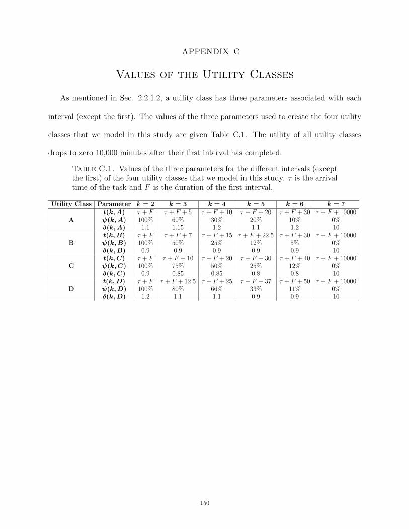
as the average execution time of the task. App. B gives the method for its computation.
App. C gives the values used to create the four utility classes.
0
1
2
+20 +40 +60
utility
time to complete after arrival
for fixedmediumpriority andmediumurgency
τ+Fτ+Fτ+Fτ+Fτ+0
Figure 2.4. The utility functions of the fourutility classes (A, B, C, and D) used in thisstudy shown at fixed priority and urgency lev-els showing the decay in utility for a task afterits arrival time τ . The duration of its first in-terval during which the utility value remainsconstant is represented by F on the x-axis.
In our simulations, the priority and ur-
gency levels of a task are set based on a joint
probability distribution that is representa-
tive of DOE/DoD environments. App. D
shows this probability distribution as a ma-
trix. The model results in most tasks having
medium and low priorities with medium and
low urgencies, and a few important tasks
having critical and high priorities with ex-
treme and high urgencies.
The values of maximum utility set by the various priority levels are: π(critical) = 8,
π(high) = 4, π(medium) = 2, and π(low) = 1. We also experimented with a different set
of values for the priority levels: π(critical) = 1, 000, π(high) = 100, π(medium) = 10, and
π(low) = 1. The exponential decay rates for the various urgency levels are: ρ(extreme) =
0.6, ρ(high) = 0.2, ρ(medium) = 0.1, and ρ(low) = 0.01. These priority and urgency values
are based on the needs of the ESSC.
2.6.3. Generating Estimated Time to Compute (ETC) Matrices. In our simu-
lation environment, we group together tasks that have similar execution time characteristics
into task types, and machines that have similar performance capabilities into machine types.
We model 100 task types and 13 machine types. In our simulations, the procedure by which
we assign tasks to task types is described in Sec. 2.6.4. We model an environment consisting
of 100 machines, where each machine belongs to one of 13 machine types. Among these 13
20
machine types, 4 are special-purpose machine types while the remaining are general-purpose
machine types. We model the special-purpose machine types as having the capability of
executing certain task types (which are special to them) approximately ten times faster than
on the general-purpose machine types. These special-purpose machine types, however, lack
the ability to execute the other task types. In our environment, three to five task types were
special on each special-purpose machine type.
We use techniques from the Coefficient of Variation (COV) method [36] to generate the
entries of the ETC matrix. The mean value of execution time on the general-purpose and the
special-purpose machine types is set to ten minutes and one minute, respectively. Complete
details about our parameters for generating ETC matrices are described in App. E. The
appendix also discusses how we distribute the 100 machines among the 13 machine types.
In this study, the task type of a task is not correlated to the worth of the task to the
system, and therefore is not related to the utility function of the task. The task type only
controls the execution time characteristics of the task.
2.6.4. Generating the Arrival Pattern of Tasks. To generate the arrival times
of the tasks in the simulation, we use different arrival patterns for the special-purpose and
the general-purpose task types. The goal of our arrival pattern generation is to closely
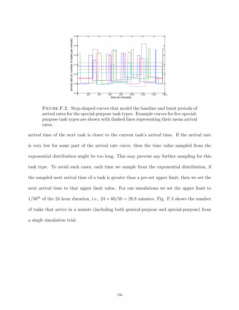
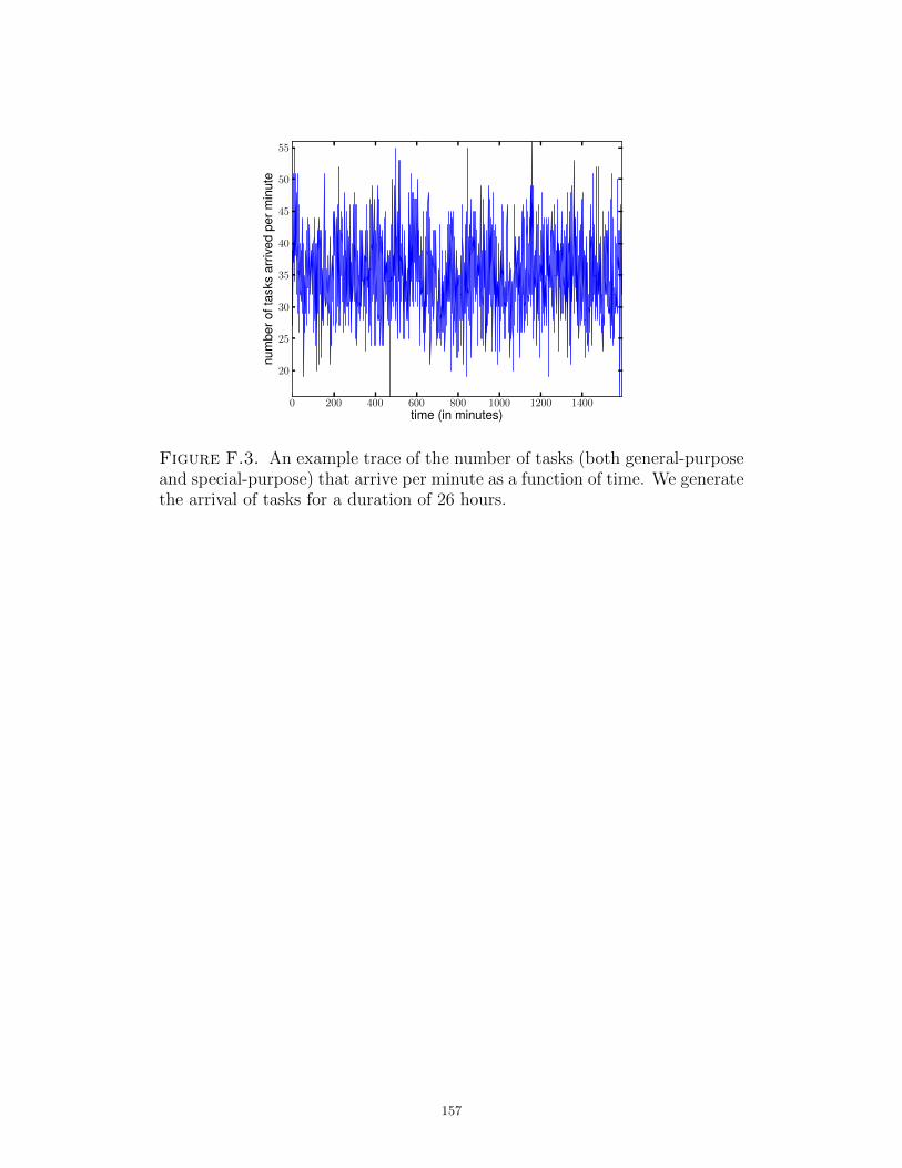
model expected workloads of DOE and DoD interest. Our simulation models the arrival and
mapping of tasks for a 24 hour period. Real-world oversubscribed systems rarely start with
empty queues. To model this in our environment, we simulate the arrival and mapping of
tasks for 26 hours, and exclude the first two hours of data from result calculations. The
initial two hours serve to bring the system up to steady-state and avoid the scenario where
the machine queues start with no tasks. We calculate all of our results (utility earned,
average heuristic execution time, number of dropped tasks, etc.) for the duration of 24
21
hours (i.e., from the end of the 2nd to the end of the 26th hour). We also model two levels
of oversubscription. In one case, approximately 33,000 tasks arrive during a 24 hour period
whereas in the other case approximately 50,000 tasks arrive over that period.
Before we generate the arrival patterns for the special-purpose and the general-purpose
tasks types, we first find a mean arrival rate of tasks for every task type (irrespective of
special-purpose or general-purpose). We find the estimated number of tasks of each task
type that will arrive during the day by sampling from a Gaussian distribution. The mean
for this distribution is the ratio of the desired number of tasks to arrive (33,000 or 50,000)
to the number of task types in the system. The variance is set to 1/10th of the mean. We
obtain the mean arrival rate of a task type by dividing the estimated number of tasks of this
task type that are to arrive during the period by 24 hours. The mean arrival rate of each
task type is used to generate arrival rate patterns (that have different arrival rates during
the 24 hours), based on whether it is a special-purpose or a general-purpose task type. For
the general-purpose task types, we use a sinusoidal pattern for the arrival rate. For the
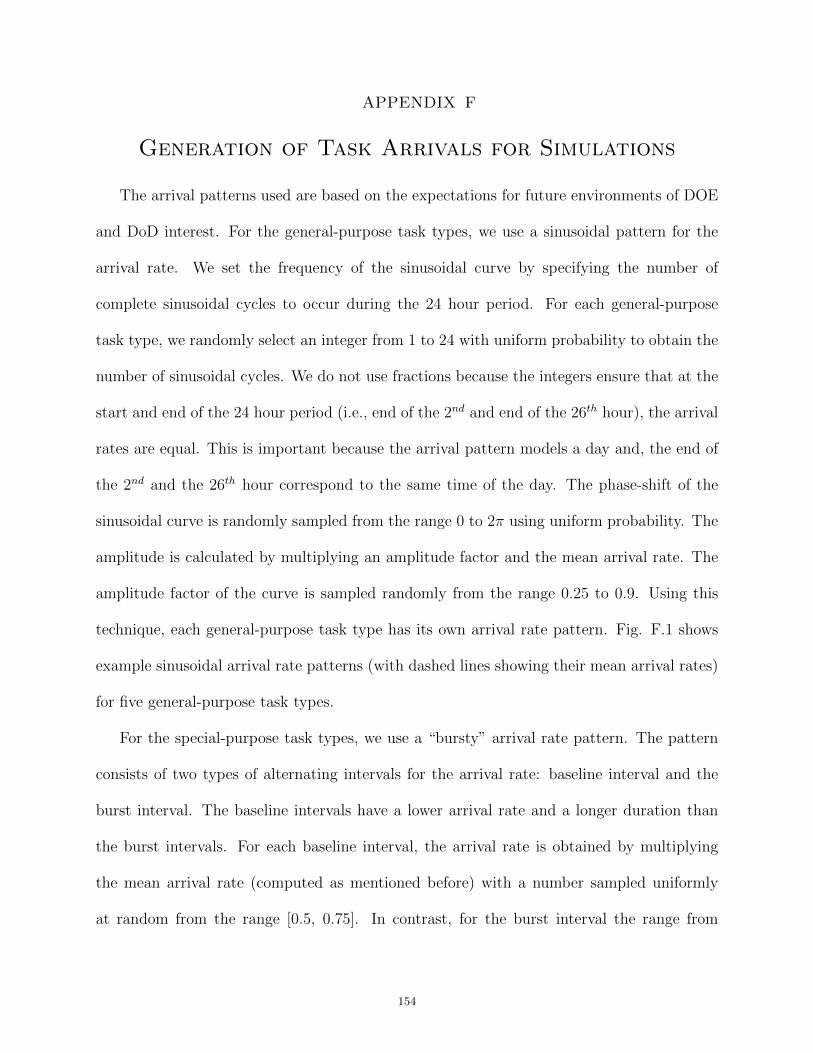
special-purpose task types, we use a bursty arrival rate pattern. App. F discusses how we
create the arrival pattern for a general-purpose or special-purpose task type, and use this
arrival rate pattern of a task type to obtain the actual number and arrival times of the tasks
belonging to that task type.
2.7. Simulation Results and Analysis
2.7.1. Overview. As mentioned in the previous section, we generate 50 simulation trials
for each experiment that we describe in this section. All bar charts in this section have results
averaged over the 50 trials with error bars showing 95% confidence intervals. For the batch-
mode heuristics, the next mapping event occurs after both of the following conditions have
22
been met: a time interval of one minute has passed since the last mapping event and the
execution of the previous mapping event has finished. Later in this section, we show results
with different methods of triggering batch-mode mapping events.
To make a fair comparison across the two levels of oversubscription, it is important to
analyze the performance of a heuristic as a percentage of the maximum possible utility that
could be achieved in that oversubscription level. The value of maximum utility bound that
can be earned is calculated by summing the utility values achieved if all tasks were assumed
to begin execution on their minimum execution time machine as soon as they arrive. We
consider only tasks whose completion times are within the 24 hour period. The values of the
maximum utility bound averaged across the 50 trials in the 33,000 and 50,000 tasks arriving
per day cases are 65,051 and 98,708, respectively. First, we compare the performance of
the various heuristics with the two levels of oversubscription. We then explore the effect of
dropping tasks with different levels of dropping thresholds.
The best value of K for the K-Best Types heuristic was empirically found to be K=1
machine type in our environment. At K=1, the K-Best Types performs the same mapping
decisions as the MET-Max Util heuristic. We therefore do not show the results from this
heuristic in any of the bar charts.
2.7.2. Preliminary Results. Fig. 2.5 shows the performance of the different heuristics
in terms of the percentage of maximum utility earned with the two levels of oversubscrip-
tion. Irrespective of the oversubscription level, we observe that the naive immediate-mode
heuristics always perform poorly compared to the smart immediate-mode heuristics. This
is because the naive heuristics do not consider ETC information, machine ready-times, and
the utility earned by a task on the various machines. The batch-mode heuristics always
perform significantly better than the smart immediate-mode heuristics. This is because the
23
batch-mode heuristics not only consider machine ready-times, but also have the ability to
schedule a set of tasks and re-map tasks that are in the virtual queues. Most of the batch-
mode heuristics are able to use this to their advantage and move any high utility-earning
task that may have just arrived to the front of the virtual queues in the next mapping event.
With the immediate-mode heuristics, the newly-arrived high utility-earning tasks would be
queued behind other tasks, and by the time they get an opportunity to execute, their util-
ity may have decayed significantly. With the 33,000 tasks per day case, on average, the
batch-mode heuristics gave an improvement of approximately 250% compared to the smart
immediate-mode heuristics.
Comparing the percentage of maximum utility earned by the heuristics for the two levels
of oversubscription shows that higher oversubscription makes it harder to earn the maximum
possible utility. The actual utility earned by a heuristic in the 50,000 tasks per day case
will typically be higher than that in the 33,000 tasks per day case. For example, the utility
earned by Min-Min Comp in the 33,000 tasks per day case is 53.13% of 65,051 = 34,555, and
in the 50,000 tasks per day case is 41.26% of 98,708 = 40,726. Even though for both levels of
oversubscription we consider the utility earned by the system only for the 24 hour duration,
the higher oversubscription rate allows a heuristic to select more higher utility earning tasks,
and therefore earn higher utility.
The Max Util and Max UPT immediate-mode heuristics earn most of their utility from
the special-purpose machines. This is because the special-purpose machines are able to
quickly execute the tasks assigned to them (i.e., special-purpose tasks) and these machines
are not oversubscribed. As a result, a task assigned to a special-purpose machine begins
execution quickly and is able to earn high utility. In contrast, the general-purpose machines
have long queues of tasks and therefore the tasks assigned to them usually earn very low
Figure 2.5. Percentage of maximum utility earned by all the heuristics undertwo levels of oversubscription: 33,000 tasks arriving within a day, and 50,000tasks arriving within a day. No tasks were dropped in these cases. The utilityearned value (as opposed to the percentage of maximum utility earned) by aheuristic in the 50,000 tasks per day case will typically be higher than that inthe 33,000 tasks per day case.
utility by the time they finish execution. MET-Random and MET-Max Util alleviate this
problem by assigning tasks to machines where they execute the fastest. This allows these
heuristics to earn utility from the general-purpose machines as well.
The performance of many batch-mode heuristics is severely affected by the increase in the
oversubscription level. The higher oversubscription results in more tasks being present in the
batch during the mapping events. With an increase in the size of the batch, the batch-mode
heuristics take considerably longer to perform each mapping event. This leads to triggering
fewer mapping events (because a new mapping event cannot begin until the previous one
completes). Fig. 2.7 shows the total number of mapping events for the batch-mode heuristics
25
under the two levels of oversubscription. The total number of mapping events are partitioned
into two sections: those triggered at the time interval of one minute and those initiated when
the execution of the previous mapping event took longer than one minute. We observe that
the batch-mode heuristics (other than Min-Min Comp in 33,000 tasks per day case) have
fewer mapping events being triggered than the expected amount (namely, 1,440 if they were
all triggered after one minute). With fewer mapping events, it takes longer for the high
utility-earning tasks to be moved up to the front of the virtual queues and the delay may
cause their utility values to decay significantly. Min-Min Comp executes faster than the other
batch-mode heuristics because it does not perform any explicit utility calculations. MET-
Max Util-Max UPT also executes relatively quickly because it performs utility calculations
only for a subset of the machines. Max-Max Util and Max-Max UPT earn very low utility
in the 50,000 tasks per day case because they have only 200 mapping events being triggered
during the day. In contrast to the batch-mode heuristics, the immediate-mode heuristics
execute quickly, and as a result, even in the case where 50,000 tasks arrive during the day,
they have approximately 50,000 mapping events with only 0.5% of those on average (250
out of 50,000) being initiated as a result of the heuristic execution of the previous mapping
event taking longer than the arrival time of the next task.
Picking the minimum execution time machine type for a task is automatically providing
load balancing in our environment. The MET-type heuristics (both immediate-mode and
batch-mode) are performing particularly well because of the high heterogeneity modeled in
our environment. If we had a variation in our environment where the workload includes
many task types that perform best on a select few machines, these MET-type heuristics
would assign all of those tasks only to these few machines resulting in long machine queues
on these fast machines, where the wait time of a task would negate the faster execution time.
26
Our level of heterogeneity is modeled based on the expectations for future environments of
DOE and DoD interest.
2.7.3. Results with Dropping Tasks. As mentioned in Sec. 2.4.4, we implement
techniques in the immediate-mode and batch-mode heuristics to drop tasks that earn utility
values less than a dropping threshold. We experiment with six levels for the dropping
threshold: 0 (which is equivalent to no dropping), 0.05, 0.5, 1.5, 3, and 5. These are chosen
based on our system model, including the values of maximum utility for the various priority
levels, i.e., 8, 4, 2, and 1. We run simulations with all the heuristics using the six dropping
thresholds for the two cases of oversubscription. In Fig. 2.6, we show the results for the
50,000 tasks per day case. The results of the 33,000 oversubscription level show similar
trends, and are discussed in App. G. The heuristics significantly benefit from the dropping
operation. For almost all heuristics, the utility earned increases as we increase our dropping
threshold from 0 to 1.5. With a dropping threshold of 1.5, all the low priority tasks are
dropped because their starting utility is 1. This may be undesirable in general, but for
our oversubscribed system this results in the best performance. The average computation
capability of our environment is such that approximately 26,000 tasks can execute in the
24-hour period (based on the average execution time of each task on each machine). Our
dropping operation lets us pick the best 26,000 tasks to execute to maximize the total utility
that can be earned. Based on a different system model and administrative policies one may
set the specific levels of dropping thresholds differently.
The immediate-mode heuristics do not have the ability to move newly arrived high-utility
earning tasks to the head of the queue because they are not allowed to remap queued tasks.
The dropping operation benefits the immediate-mode heuristics by clearing the machine
queues of the lower-utility-earning tasks, which allows the other queued tasks to execute
Figure 2.6. Percentage of maximum utility earned earned by all the heuris-tics for the different dropping thresholds with the oversubscription level of50,000 tasks arriving during the day. The average maximum utility bound forthis oversubscription level is 98,708.
sooner and earn higher utility. This helps the immediate-mode heuristics to earn utility
from the general-purpose machines. The special-purpose machines were not oversubscribed
and therefore there is no significant increase in performance from these machines because of
the dropping operation. At the best dropping threshold, i.e., 1.5, Max Util and Max UPT
have an approximately 450% performance improvement compared to the no dropping case.
The performance of these two heuristics comparable to that of the batch-mode heuristics.
As we increase the dropping threshold beyond 1.5, we drop too many tasks from our system
and as a result earn less utility overall.
There are two main reasons why the batch-mode heuristics benefit from the dropping
operation. The first is that the dropping operation helps them reduce the size of their batch
28
during each mapping event by dropping tasks that would only be able to earn low utility.
This makes the mapping events execute faster and results in more mapping events. For the
batch-mode heuristics, in all cases where some level of dropping was implemented, all of the
1440 mapping events were triggered. With the increase in the number of mapping events,
the batch-mode heuristics are able to service high utility-earning tasks faster. This causes
the improvement in performance in the dropping at 0.05 case compared to the no dropping
case. The second reason the batch-mode heuristics benefit from the dropping operation is
the prevention of low utility-earning tasks from blocking the pending and the executing slots
of the machines. When tasks are arriving, there may be periods when most of the arriving
tasks are neither critical nor high priority tasks. During this time period, other lower priority
tasks get the opportunity to fill into the pending slots of the machines. If there is a burst of
critical or high priority tasks after this period, these higher-priority tasks will have to wait
in queue behind the lower priority task in the pending slot, because the pending slot tasks
cannot be re-mapped. By dropping the lower priority tasks, we do not block the pending
(and hence the executing) slots and when the high utility-earning tasks arrive they get to
quickly start execution and provide higher utility to the system. This causes the performance
improvement for batch-mode heuristics with further dropping beyond 0.05. Similar to the
immediate-mode heuristics, dropping thresholds greater than 1.5 drop too many tasks.
Max-Max Util, Max-Max UPT, and MET-Max Util-Max UPT maximize the utility
earned and push low utility-earning tasks to the back of the queue. Thus, for these heuristics,
the biggest advantage of the dropping operation is to reduce the size of the batch, allowing
for more mapping events.
The dropping operation also helps to make the Min-Min Comp and Sufferage heuris-
tics more utility-aware, and we get the biggest performance improvement by increasing the
29
dropping threshold to 1.5 (even though the dropping threshold at 0.05 triggered all 1,440
mapping events).
In all cases where some level of dropping is implemented, almost all of the heuristics
earn similar values of utility from the special-purpose machines because these machines are
not oversubscribed. Utility earned from special-purpose machines decreases with dropping
thresholds of 1.5 and higher because proportionally the number of special-purpose tasks
become fewer.
Although the smart immediate-mode heuristics can earn utility comparable to the batch-
mode heuristics, their performance is very sensitive to the value of the dropping threshold.
For the immediate-mode heuristics, the dropping threshold parameter needs to be tuned
based on the starting utility values for the different priority levels, arrival pattern of the
tasks, degree of oversubscription of the environment, etc., because the immediate-mode
heuristics rely on the dropping threshold to empty the machine queues. In contrast, the
mechanism by which the dropping operation helps batch-mode heuristics such as Max-Max
Util, Max-Max UPT, and MET-Max Util-Max UPT is different, i.e., it increases the number
of mapping events. The performance of these batch-mode heuristics is less sensitive to the
value of the dropping threshold.
The MET-based heuristics, i.e., MET-Random, MET-Max Util, and MET-Max Util-
Max UPT, earn less utility compared to the other heuristics at a dropping threshold of 1.5.
At this dropping threshold, all the low priority tasks are dropped from the system, and
they account for approximately 53% of tasks (see App. D). Therefore, with a 1.5 dropping
threshold the degree of oversubscription reduces significantly. The MET-based heuristics
assign tasks to the machines that belong to the best execution time machine type. As a
result, these heuristics hurt their case at this dropping threshold by oversubscribing certain
30
machines. This causes them to drop more tasks (because tasks wait longer) compared to
the other heuristics and earn less utility overall. The effect of increased oversubscription
by the MET-based heuristics is not apparent at the 0.5 and 3 dropping thresholds because
at these dropping thresholds the system is much more oversubscribed and undersubscribed,
respectively.
For dropping thresholds 1.5 and above, almost all the heuristics earn similar amounts
of total utility (except naive heuristics and the MET-based heuristics). At these dropping
thresholds, only tasks of higher priority levels are executing on the machines (as tasks with
lower priority levels have starting utility values less than the dropping threshold) and as a
result the degree of oversubscription is reduced. The non-dropped tasks start execution as
soon as they because machines are idle most of the time, and therefore, all heuristics earn
similar levels of utility.
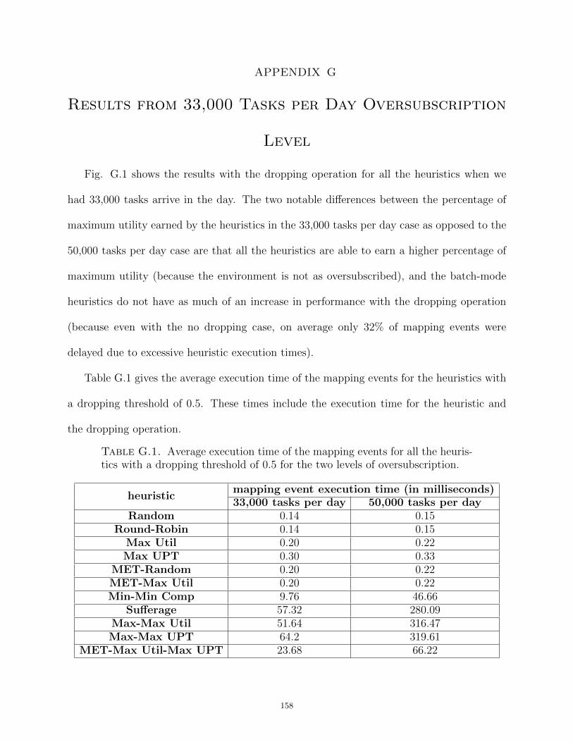
The average mapping event execution times for the heuristics in both levels of over-
subscription at a 0.5 dropping threshold are in App. G. Results of experiments with the
maximum utility values for the priority levels set at 1000, 100, 10, and 1 are discussed in
App. H.
2.7.4. Triggering Batch-mode Mapping Events. The ability of the batch-mode
heuristics to update the machine queues with a high utility-earning task that may have
arrived recently provides a distinct advantage. We now study the effect of varying the size of
the batch by exploring other possibilities for triggering the next mapping event. We examine
a technique to trigger batch-mode mapping events based on a combination of time interval
and number of tasks that have arrived since the last mapping event. A mapping event will
be triggered when either of the above (time interval or number of tasks) occur, or after
the previous mapping execution if it takes longer. These studies are performed using the
31
0.5 dropping threshold and 50,000 tasks per day case. We experiment with the following
five triggering cases: (1) number of tasks: 1; (2) number of tasks: 2, or time interval:
0.0576 minutes; (3) number of tasks: 35, or time interval: 1 minute; (4) number of tasks:
70, or time interval: 2 minutes; (5) number of tasks: 347, or time interval: 10 minutes.
For each case, the time intervals are chosen to approximate the corresponding estimated
number of task arrivals. These experiment parameters are set based on our simulation
environment. One could perform such tests with different values for the parameters based
on other environments.
Fig. 2.8 shows the performance of the Max-Max UPT heuristic with the different cases
of triggering. The other batch-mode heuristics show similar trends as the Max-Max UPT
heuristic. In all five triggering cases mentioned above and for all of the batch-mode heuristics,
the average execution time of a mapping event with a dropping threshold of 0.5 is under 350
milliseconds.
The best performance is obtained when mapping events keep triggering every time a
new task arrives. The batch-mode heuristics were able to execute 50,000 mapping events
because we are using a dropping threshold of 0.5 and this makes the heuristics execute
quickly. The performance benefit is due to the heuristics being able to use new information
to quickly re-map tasks. However, the increase in performance is small because very few
tasks among the newly arrived tasks would be critical or high priority tasks. It is usually
the high utility-earning tasks that change the mapping of the previously mapped tasks. As
mentioned in App. D, on average approximately 4% and 11% of tasks are critical and high
priority tasks, respectively. Therefore, after a minute or after 35 task arrivals, there would
probably be approximately one critical and four high priority tasks among the newly arrived
32
Min-Min Comp
Sufferage
Max-Max Util
Max-Max UPT
MET-Max Util-
Max UPT
batch-mode heuristics
0
200
400
600
800
1000
1200
1400
1600
num
bero
fmap
ping
even
ts(a
vera
ged
over
50tr
ials
)
text
33,0
00ta
sks/
day
case
text
50,0
00ta
sks/
day
case
ooo
initi
ated
afte
rpre
viou
sm
appi
ngev
ent
///
trig
gere
dat
time
inte
rval
Figure 2.7. The number of mappingevents initiated either because the oneminute time interval has passed since thelast mapping event or because the previ-ous mapping event finished execution af-ter one minute are shown for five batch-mode heuristics with the two levels ofoversubscription: 33,000 tasks arrivingwithin a day, and 50,000 tasks arrivingwithin a day. No tasks were dropped inthese cases.
tasks. Scheduling these as soon as they arrive instead of waiting for less than a minute
provides only a marginal increase in the total performance.
2.8. Conclusions and Future Work
In this study, we develop a flexible metric that uses utility functions to compare the
performance of resource allocation heuristics in an oversubscribed heterogeneous computing
environment where tasks arrive dynamically throughout a 24 hour period. We model this
type of environment based on the needs of the ESSC at ORNL. We design and analyze the
33
performance of seven immediate-mode heuristics and five batch-mode heuristics in our sim-
ulated environment based on the total utility they could earn during a one day time period.
We observe that without the ability to drop tasks, the naive immediate-mode heuristics per-
form poorly compared to the smart immediate-mode heuristics, which in turn perform poorly
compared to the batch-mode heuristics. Among the batch-mode heuristics, Max-Max UPT
and MET-Max Util-Max UPT perform the best. This is because these batch-mode heuristics
consider the minimization of the execution time of the task in addition to maximizing util-
ity. This is helpful in an oversubscribed highly heterogeneous environment. Dropping low
utility-earning tasks significantly helps improve performance of the immediate-mode heuris-
tics because it allows other relatively high-utility earning tasks to execute sooner and thus
earn more utility. Dropping tasks also improves the batch-mode heuristics in two ways, (a)
by preventing large batch sizes which results in more mapping events being triggered due
to faster heuristic execution times, and (b) by preventing lower-priority tasks from enter-
ing into the pending slot so that higher priority tasks that arrive subsequently can execute
sooner. Immediate-mode heuristics are much more sensitive to the value of the dropping
threshold and rely on its tuning to avoid low utility earning tasks from entering machine
queues. Permuting the initial tasks at the head of the virtual queues does not affect the
performance significantly in our environment. We also experiment with different triggers for
the batch-mode mapping events. We observe that (in our environment) triggering every time
a new task arrives is not providing significant benefit in the total utility earned compared
to mapping after every minute. Possible future directions for this research are mentioned in
Chapter 6.
34
CHAPTER 3
Trade-offs Between System Performance and
Energy Consumption2
3.1. Introduction
During the past decade, large datacenters (comprised of supercomputers, servers, clus-
ters, farms, storage, etc.) have become increasingly powerful. As a result of this increased
performance the amount of energy needed to operate these systems has also grown. It was
estimated that between the years 2000 and 2006 the amount of energy consumed by high
performance computing systems more than doubled [38]. In 2006 an estimated 61 billon
kWh was consumed by servers and datacenters, approximately equal to 1.5% of the total
United States energy consumption for that year. This amounted to $4.5 billion in electricity
costs [38]. Since 2005, the total amount of electricity used by HPC systems increased by
another 56% worldwide and 36% in the U.S. Additionally, during 2010, global HPC systems
accounted for 1.5% of total electricity use, while in the U.S., HPC systems accounted for
2.2% [2].
With the cost of energy and the need for greater performance rising, it is becoming
increasingly important for HPC systems to operate in an energy-efficient manner. One way
to reduce the cost of energy is to minimize the amount of energy consumed by a specific
system. In this work, we show that we can reduce the amount of energy consumed by a
system by making intelligent scheduling decisions. Unfortunately, consuming less energy
2This work was done jointly with Ph.D. student Ryan Friese. The full list of co-authors is at [37]. Thisresearch used resources of the National Center for Computational Sciences at Oak Ridge National Laboratory,supported by the Extreme Scale Systems Center at ORNL, which is supported by the Department of Defenseunder subcontract numbers 4000094858 and 4000108022. This research also used the CSU ISTeC CraySystem supported by NSF Grant CNS-0923386.
35
often leads to a decrease in the performance of the system [39]. Thus, it can be useful to
examine the trade-offs between minimizing energy consumption and maximizing computing
performance for different resource allocations. Current resource managers, such as MOAB,
cannot reasonably determine the trade-offs between performance and energy.
In this research, we model a computing environment and corresponding workload that
is being investigated by the Extreme Scale Systems Center (ESSC) at Oak Ridge National
Laboratory (ORNL). The ESSC is a joint venture between the United States Department
of Defense (DoD) and Department of Energy (DOE) to provide research, tools, software,
and technologies that can be utilitized in both DoD and DOE environments. Our goal
is to design an analysis framework that a system administrator can use to analyze the
energy and performance trade-offs of a system by using different resource allocations (i.e.
mapping of tasks to machines). System performance is measured in terms of total utility
earned, where each task in the workload is assigned a time utility function that monotonically
decreases in value the longer a task remains in the system [4]. The computing environment
is a heterogeneous mix of machines and tasks that represents an environment with system
characteristics and workload parameters that are based on the expectations of future DoD
and DOE environments.
In a heterogeneous environment, tasks may have different execution and power consump-
tion characteristics when executed on different machines. One can change the performance
and energy consumption of the system by using different resource allocations. A resource
allocation is defined to be a complete mapping of tasks to machines, where we assume the
number of tasks is much greater than the number of machines. To create these resource
allocations, we model this scheduling problem as a bi-objective optimization problem that
36
maximizes utility earned and minimizes energy consumed. We adapt the Nondominated
Sorting Genetic Algorithm II (NSGA-II) [40] to create the resource allocations.
To analyze the effect of different resource allocations, we implement our method in a
static and offline environment. To create the offline environment we simulate a trace over
a specified time period of the modeled environment. This allows us to gather information
about the number of tasks that arrived during this time period, as well as the arrival times
and types of tasks that were present in the system. The availability of this information
makes this a static resource allocation problem. The knowledge gained from studies such
as this can be used to set the parameters needed for designing dynamic or online allocation
heuristics.
We utilize execution and power consumption characteristics from real machines and ap-
plications. We further use this real characteristic data to create a larger data set in order to
simulate larger systems. In all cases, our results show that by using different resource allo-
cations a system administrator can greatly change the amount of utility earned and power
consumed based on the needs of their system.
In this chapter we make the following contributions:
(1) Modeling a bi-objective resource allocation problem between total utility earned
and total energy consumed to address concerns about energy-efficient computing,
specifically for environments of DoD and DOE interest.
(2) Creating and evaluating many intelligent resource allocations to show that the utility
earned and energy consumed by the system can change greatly.
(3) Demonstrating our method by using real machine and task data.
(4) Providing a method to create synthetic data sets that preserve the heterogeneity
measures found from real data sets.
37
(5) Analyzing the effect of using different seeding heuristics on the evolution of solutions
found by the genetic algorithm.
The remainder of this chapter is organized as follows. Related work is discussed in Section
3.2. We construct the system model, and our real data set, in Section 3.3. In Section 3.4, we
describe our bi-objective optimization problem and the NSGA-II. Our simulation setup is
Let Tm be the tasks that execute on machine m, where task tm ∈ Tm. The total energy
consumed by the system, denoted E, is found by
(5) E =∑∀m∈M
∑∀tm∈Tm
EEC[Φ(tm),Ω(m)].
47
Figure 3.1. Task time-utility function showing values earned at differentcompletion times.
3.4.3. Generating Solutions for a Bi-Objective Optimization Problem. When
a problem contains multiple objectives, it is challenging to determine a single global optimal
solution. Often, there is instead a set of optimal solutions. This set of optimal solutions
may not be known, thus it is important to find a set of solutions that are as close as possible
to the optimal set. The set of solutions that we find that best approximates the optimal
set is called the set of Pareto optimal solutions [52]. The Pareto optimal set can be used to
construct a Pareto front that can illustrate the trade-offs between the two objectives.
Not all solutions we find can exist within the Pareto optimal set. We select the eligible
solutions by examining solution dominance. Dominance is used to compare two solutions
to one another. For one solution to dominate another, it must be better than the other
solution in at least one objective, and better than or equal in the other objective. Figure 3.2
illustrates the notion of solution dominance. In this figure we show three potential solutions:
A, B, and C. The objectives we are optimizing for are minimizing total energy consumption
along the x-axis and maximizing total utility earned along the y axis. A “good” solution
would be one that consumes small amounts of energy and earns large amounts of utility
(upper left corner).
48
energy consumed
utility A B
C
solutions that dominate A
solutions that are dominated by A
Figure 3.2. Illustration of solution dominance for three solutions: A, B, andC. Solution A dominates solution B because A has lower energy consumptionas well as it earns more utility. Neither solution A nor C dominate each otherbecause C uses less energy, while A earns more utility.
If we consider solutions A and B, we can say that B is dominated by A. This is because
A uses less energy as well as earns more utility than B. The same is true for any solution
located within the lower right region. Now, when we examine solutions A and C we cannot
make any claims on the dominance of one solution over the other. This is because C uses
less energy than A, but C does not earn as much utility, thus the two solutions can not be
directly compared to each other, which means they are both located on the Pareto front.
Finally, solution A will only be dominated by solutions that exist in the upper left region.
3.4.4. Nondominated Sorting Genetic Algorithm II. The Nondominated Sort-
ing Genetic Algorithm II (NSGA-II) was designed for solving bi-objective optimization prob-
lems [40]. We adapt a version of the NSGA-II that we used in [39] for a different, simpler
resource allocation problem. We will briefly describe the basic NSGA-II algorithm and how
we have modified it for our specific problem.
The NSGA-II is a popular multi-objective genetic algorithm that utilizes solution dom-
inance to allow the populations of chromosomes to evolve into better solutions over time.
49
For our problem domain, a single population represents a set of possible resource allocations
(solutions). To use the NSGA-II for our problem we needed improve upon [39] and encode
the algorithm so that it could solve bi-objective resource allocation problems where the two
objectives are maximizing utility earned and minimizing energy consumed. To do this, the
algorithm must be able to accurately track and calculate the individual utility earned by
each task. This meant we needed to create our own genes, chromosomes, crossover operator,
and mutation operator.
Genes represent the basic data structure of the genetic algorithm. For our problem, a
gene represents a task. Each gene contains: the machine the gene will operate on, the arrival
time of the task, and the global scheduling order of the task. The global scheduling order is
a number from 1 to the number of tasks in the chromosome and it controls the order that
tasks execute on the individual machines. The lower the number, the sooner the task will
execute. The global scheduling order is independent of the task arrival times.
A chromosome represents a complete solution, i.e., resource allocation. Each chromosome
is comprised of T genes, where T is the number of tasks that are present in the trace being
studied. The ith gene in every chromosome corresponds to the same task, in particular, the
ith task ordered based on task arrival times. To examine dominance relationships amongst
the chromosomes in the population, each chromosome is individually evaluated with respect
to utility earned and energy consumed. Because the global scheduling order is independent
of task arrival times, we must ensure that any task’s start time is greater than or equal to
its arrival time. If this is not the case, the machine sits idle until this condition is met.
For populations and chromosomes to evolve from one generation to the next, the following
crossover and mutation operations were implemented. For crossover, we first select two
chromosomes uniformly at random from the population. Next, the indices of two genes
50
are selected uniformly at random from within the chromosomes. Finally, we swap all the
genes between these two indices, from one chromosome to the other. In this operation, the
machines the tasks execute on, and the global scheduling orders of the tasks are all swapped.
The goal of this operation is to allow chromosomes making good scheduling decisions to pass
on favorable traits to other chromosomes.
For the mutation operation, we randomly select a chromosome from the population. We
then select a random gene from within that chromosome. We then mutate the gene by
selecting a random machine that that task can execute on. Additionally, we select another
random gene within the chromosomes and then swap the global scheduling order between
the two genes.
Within a given population, a solution is ranked based on how many other solutions
dominate it. If no other solutions dominate a solution, it is said to be nondominated and is
given a rank of 1. A solution’s rank can be found by taking 1 + the number of solutions that
dominate it. All solutions of rank 1 within a given population represent the current Pareto
optimal set. The process of sorting the solutions is performed using the nondominating
sorting algorithm, and is one step of the NSGA-II algorithm. A basic outline of the NSGA-
II is taken from [39] and shown in Algorithm 1.
An important step to understand in the algorithm is the creation of offspring populations
(step 3). We start with a parent population of size N. We then perform N/2 crossover
operations (each crossover operation produces two offspring) to produce an initial offspring
population also of size N. Next, the mutation operation is then performed with a probability
(selected by experimentation) on each offspring within the population. If a mutation occurs,
only the mutated offspring remains in the population.
51
Algorithm 1 NSGA-II algorithm from [39]
1: create initial population of N chromosomes2: while termination criterion is not met do3: create offspring population of size N4: perform crossover operation5: perform mutation operation6: combine offspring and parent populations into a single meta-population of
size 2N7: sort solutions in meta-population using nondominated sorting algorithm8: take all of the rank 1, rank 2, etc. solutions until we have at least N
solutions to be used in the parent population for the next generation9: if more than N solutions then10: for solutions from the highest rank number used, take a subset based
on crowding distance [40]11: end if12: end while13: the final population is the Pareto front used to show the trade-offs between the two
objectives
We can now combine the parent and offspring population into a single meta-population
of size 2N (step 6). This combining of populations allows elitism to be present within the
algorithm, that is the algorithm keeps the best chromosomes from the previous generation
and allows them to be evaluated in the current generation. From this new meta-population,
we then select the next generation’s parent population (steps 7, 8, 9, and 10). To create the
new parent population, we need to select the best N chromosomes from the meta-population.
To illustrate this procedure, we provide the following example. Assume we currently have
a parent population and offspring population, each with 100 chromosomes, which combines to
make a meta-population with 200 chromosomes. We then perform the nondominated sorting
algorithm from step 7. We find that we have 60 chromosomes of rank 1, 30 chromosomes of
rank 2, 20 chromosomes of rank 3, and 90 chromosomes that have a rank higher than 3. We
need to create a new parent population with only 100 chromosomes in it. First we take the
60 chromosomes that are rank 1 and place them into the new population. This leaves room
for 40 more chromosomes. We then place the rank 2 chromosomes in the new population.
52
There is space in the population for 10 additional chromosomes. To select only 10 out of
the 20 rank 3 chromosomes we use the method of crowding distance [40] to arrive at our
full 100 chromosome population. Crowding distance is a metric that penalizes chromosomes
that are densely packed together, and rewards chromosomes that are in remote sections of
the solutions space. This operation creates a more equally spaced Pareto front.
3.5. Simulation Setup
3.5.1. Datasets and Experiments. To illustrate how our analysis framework allows
system administrators to analyze the trade-offs between utility earned and energy consumed
of a given system, we have conducted numerous simulations using three different sets of data.
The first set consists of the real historical ETC and EPC data gathered from the online
benchmarks (nine machine types and five task types) [49]. This set only allotted one machine
to each machine type and simulated 250 tasks comprised of the five task types arriving over
a period of 15 minutes. We are performing a post-mortem static resource allocation as we
are using a trace of a (simulated) system, thus the arrival times of all tasks are known a
priori. This real data set is used as the basis for the second and third data sets, as described
is Subsection 3.3.4.2.
The second and third sets consist of the ETC and EPC data manufactured from the
real data (Subsection 3.3.4.2). For these sets, we created four special-purpose machine types
for a total of 13 machine types and 25 additional task types for a total of 30 task types.
Additionally, for both sets there were 30 machines across the 13 machine types. The break
up of those machines can be seen in Table 3.3. Data sets 2 and 3 differ from one another by
the number of tasks each set simulates. Set 2 simulates 1000 tasks arriving within the span
of 15 minutes, while set 3 simulates 4000 tasks arriving within the span of an hour.
53
Table 3.3. Breakup of machines to machine types
machine type number of machines
Special-purpose machine A 1Special-purpose machine B 1Special-purpose machine C 1Special-purpose machine D 1
We conducted experiments on each data set. For the first group of experiments, we let
the genetic algorithm execute for a given number of generations and then we analyze the
trade-offs between utility earned and energy consumed. The second group of experiments
compare the effect of using different seeds within the initial population on the evolution of
the Pareto fronts. The seeding heuristics used for these experiments are described in the
section below.
3.5.2. Seeding Heuristics. Seeding heuristics provide the genetic algorithm with ini-
tial solutions that try to intelligently optimize one or both of the objectives. The seeds may
help guide the genetic algorithm into better portions of the search space faster than an all
random initial population. We implement the following four heuristics: Min Energy, Max
Utility, Max Utility-per-Energy, and Min-Min Completion Time. The execution times of the
greedy heuristics are negligible compared to the NSGA-II, making solutions found by these
heuristics plausible to use. To use a seed within a population, we generate a new chromo-
some from one of the following heuristics. We place this chromosome into the population
and create the rest of the chromosomes for that population randomly.
54
3.5.2.1. Min Energy. Min Energy is a single stage greedy heuristic that maps tasks to
machines that minimize energy consumption. This heuristic maps tasks according to their
arrival time. For each task the heuristic maps it to the machine that consumes the least
amount of energy to execute the task. This heuristic will create a solution with the minimum
possible energy consumption. Solutions may exist that consume the same amount of energy
while earning more utility.
3.5.2.2. Max Utility. Max Utility is also a single stage greedy heuristic similar to the min
energy heuristic except that it maps tasks to the machines that maximizes utility earned
[4]. This heuristic must consider the completion time of the machine queues when making
mapping decisions. There is no guarantee this heuristic will create a solution with the
maximum obtainable utility.
3.5.2.3. Max Utility-per-Energy. Max Utility-per-Energy tries to combine aspects of the
previous two heuristics. Instead of making mapping decisions based on either energy con-
sumption or utility earned independently, this heuristic maps a given task to the machine
that will provide the most utility earned per unit of energy consumed.
3.5.2.4. Min-Min Completion Time. Min-min completion time is a two-stage greedy
heuristic that maps tasks to the machines that provide the minimum completion time
[20, 53, 11]. During the first stage, the heuristic finds for every task the machine that
minimizes that task’s completion time. In the second stage, the heuristic selects from among
all the task-machine pairs (from the first stage) the pair that provides the overall minimum
completion time. That task is then mapped to that machine, and the heuristic repeats this
operation until there are no more tasks to map.
55
3.6. Results
In Figures 3.3, 3.4, and 3.6 we show the location of numerous Pareto fronts. In each
figure we show different fronts corresponding to different initial populations, for each of our
three data sets respectively. Each of the four subplots show the Pareto fronts through a
specific number of NSGA-II iterations. The x-axis is the number of megajoules consumed
by the system, and the y-axis is the amount of utility earned by the system. Each marker
within the subplots represents a complete resource allocation. Each marker style represents a
different population. The diamond marker represents the population that contained the “Min
Energy” seed, the square marker represents the population with the “Min-Min completion
time” seed, the circle marker represents the population with the “Max Utility” seed, the
triangle maker represents the population with the “Max Utility-per-Energy” seed, and finally
the star marker represents the population with a completely random initial population. We
also considered an initial population that contained all four of the seeding heuristics, but
we found that this population performed similarly to the min-energy seeded population, and
thus did not include it in our results.
Figure 3.3 shows the Pareto fronts for the real historical data set. For this data set we
evaluated the evolution of the Pareto fronts through four different number of iterations; 100,
1000, 10,000, and 100,000 iterations. First, in the top left subplot we see that after 100
iterations the populations have formed distinct Pareto fronts covering various parts of the
solution space. This occurs because of the use of the different seeds within each population.
The presence of the seed within a population allows that population to initially explore
the solution space close to where the seed originated. As the number of iterations increase
though, the presence of the seed starts to become irrelevant because all the populations,
even the all random initial population, start converging to very similar Pareto fronts.
56
min energy seeded populationmax utility seeded populationmax utility-per-energyseeded populationmin-min completion time seeded population
Figure 3.3. Pareto fronts of total energy consumed vs. total utility earnedfor the real historical data set (data set 1) for different initial seeded popula-tions through various number of iterations. The circled region represents thesolutions that earn the most utility per energy spent. The y-axis values areshared across subplots and while the x-axis values are specific to each subplot.
In the 100,000 iteration subplot, the region highlighted by the circle represents the so-
lutions that earn the most utility per energy consumed. This circle does not represent the
best solution in the front, because all solutions along the front are best solutions, each repre-
senting a different trade-off between utility and energy. The system administrator may not
have energy to reach the circled solution, or may be willing to invest more energy for more
utility. To the left of this region, the system can earn relatively larger amounts of utility for
relatively small increases in energy. To the right of this region, the system could consume a
relatively larger amount of energy but would only see a relatively small increase in utility.
A system administrator can use this bi-objective optimization approach to analyze the
utility-energy trade-offs for any system of interest, and then set parameters, such as energy
constraints, according to the needs of that system. These energy constraints could then be
used in conjunction with a separate online dynamic utility maximization heuristics.
57
min energy seeded populationmax utility seeded populationmax utility-per-energyseeded population
all random initial population
min-min completion time seeded population
Figure 3.4. Pareto fronts of total energy consumed vs. total utility earnedfor the data set containing 1000 tasks (data set 2) for different initial seededpopulations through various number of iterations. The circled region repre-sents the solutions that earn the most utility per energy spent. Both the y-axisand x-axis values are specific to each subplot.
A B C
Figure 3.5. Subplot A shows the Pareto front through 1,000,000 iterationsfor the “max utility-per-energy” seeded population. The circled region rep-resents the solutions that earn the most utility per energy spent. Subplot Bprovides the utility value that gives the highest utility earned per energy spent,shown by the solid line. Subplot C provides the energy value that gives thehighest utility earned per energy spent, shown by the dashed line.
The Pareto fronts in Figure 3.4 illustrate the trade-offs between total energy consumed
and total utility earned for the data set that contains 1000 tasks. These fronts were evaluated
at 1000, 10,000, 100,000, and 1,000,000 iterations. We increased the number of iterations
58
min energy seeded poputationmax utility seeded poputationmax utility-per-energyseeded poputation
all random initial poputation
min-min completion time seeded poputation
Figure 3.6. Pareto fronts of total energy consumed vs. total utility earnedfor the data set containing 4000 tasks (data set 3) for different initial seededpopulations through various number of iterations. The circled region repre-sents the solutions that earn the most utility per energy spent. Both the y-axisand x-axis values are specific to each subplot.
executed for this data set compared to the real historical data set because we are simulating
a larger and more difficult problem.
Examining the top two subplots, we see the effect the initial seeds have on each of the
populations. This provides the chance for system administrators to make some interesting
observations about their systems. For example, the “min energy” population typically finds
solutions that perform better with respect to energy consumption, while the “min-min com-
pletion time” population typically finds solutions that perform better with respect to utility
earned. This analysis could provide insight into what type of dynamic heuristics could be
used to either maximize utility or minimize energy depending on the needs of a given sys-
tem. These subplots also show that using smart resource allocation seeds can produce better
solutions in a limited number of iterations
59
In the lower two subplots, we see that all the populations have started to converge
towards the same Pareto front. This allows us to find the region containing the solutions
that earn the most utility per energy and can provide system administrators with valuable
information about the trade-offs between the total energy consumed and the total utility
earned of their specific systems. Figure 3.5 illustrates how the maximum utility per energy
region is found. Subplot 3.5.A shows the final Pareto front for the “max utility-per-energy”
seeded population. Subplot 3.5.B shows a plot of utility earned per energy spent vs. utility
while Subplot 3.5.C shows a plot of utility earned per energy spent vs. energy. By locating
the “peaks” in both these plots we can find the utility and energy values, respectively, for
which utility earned per energy spent is maximized. We can then translate these values onto
the Pareto front to find where this region is located. This is shown using the solid lines for
utility and the dashed lines for energy.
Finally, Figure 3.6 contains the Pareto fronts for the largest of our three data sets (4000
tasks). This data set is also evaluated at 1000, 10,000, 100,000, and 1,000,000 iterations.
Due to the larger size of this problem, it takes more iterations for the Pareto fronts to start
converging. This allows us to see the benefit of using the seeds in the initial populations over
the all random initial population. In all cases, our seeded populations are finding solutions
that dominate those found by the random population. This occurs because the random initial
population has to rely on only crossover and mutation to find better solutions, whereas the
seeded populations have the advantage of a solution that is already trying to make smart
resource allocation decisions.
Similar to the first two data sets, we see that Pareto fronts for this data set also exhibit
a region where the amount of utility earned per energy spent is maximized. This is the
60
location where the system is operating as efficiently as possible, and can help guide system
administrators in making decisions to try and reach that level of efficiency for their systems.
3.7. Conclusions
Rising costs of energy consumption and the push for greater performance make the
need for energy-efficient computing very important as HPC continues to grow. To begin
computing in an energy-efficient manner, system administrators must first understand the
energy and performance characteristics of their systems. In this work, we have provided
an analysis framework for investigating the trade-offs between total utility earned and total
energy consumed. We have developed a method for creating a synthetic data set that
preserves the heterogeneity characteristics of a data set constructed from real historical
data.
We showed that by using the NSGA-II we can create well defined Pareto fronts and
analyzed how using different seeding heuristics within the initial populations affected the
evolution of the Pareto fronts. Finally, we tested our method using three data sets. The
first data set contained only real data gathered from online benchmarks. The other two
data sets contained synthetic data created from the real data to simulate a larger computing
system. These two data sets differed in the number of tasks that were required to execute.
Our method successfully illustrates the trade-offs between energy consumption and utility
earned for all three data sets. Possible future work are mentioned in Chapter 6.
In summary we have designed an analysis framework that: 1) provides the ability to
create synthetic data sets that preserve the heterogeneity measures found from real data
sets, 2) provides the ability to take traces from any given system and then use our resource
allocation heuristic and simulation infrastructure to plot and analyze the trade-offs between
61
total utility earned and total energy consumed, 3) find the region of the Pareto front where
a given system is operating as efficiently as possible, and 4) show the effect different genetic
algorithm seeds have for various systems, and how using seeds can create populations that
dominate completely random populations.
62
CHAPTER 4
Energy Constrained Utility Maximization3
4.1. Introduction
During the past decade, large-scale computing systems have become increasingly power-
ful. As a result, there is a growing concern with the amount of energy needed to operate
these systems [56, 57]. An August 2013 report by Digital Power Group estimates the global
Information-Communications-Technologies ecosystem’s use of electricity was approaching
10% of the world electricity generation [58]. As another energy comparison, it was using
about 50% more energy than global aviation [58]. In 2007, global data center power require-
ments were 12 GW and in the four years to 2011, it doubled to 24 GW. Then, in 2012 alone
it grew by 63% to 38 GW according to the 2012 DatacenterDynamics census [59]. Some
data centers are now unable to increase their computing performance due to physical limita-
tions on the availability of energy. For example, in 2010, Morgan Stanley, a global financial
services firm based in New York, was physically unable to draw the energy needed to run a
data center in Manhattan [60]. Many high performance computing (HPC) systems are now
being forced to execute workloads with severe constraints on the amount of energy available
to be consumed.
The need for ever increasing levels of performance among HPC systems combined with
higher energy consumption and costs are making it increasingly important for system ad-
ministrators to adopt energy-efficient workload execution policies. In an energy-constrained
3This work was done jointly with the Ph.D. student Ryan Friese. The full list of co-authors is at [54]. Apreliminary version of portions of the work mentioned in this chapter appeared in [55]. This research usedresources of the National Center for Computational Sciences at Oak Ridge National Laboratory, supportedby the Extreme Scale Systems Center at ORNL, which is supported by the Department of Defense undersubcontract numbers 4000094858 and 4000108022. This research also used the CSU ISTeC Cray Systemsupported by NSF Grant CNS-0923386.
63
environment, it is desirable for such policies to maximize the performance of the system.
This research investigates the design of energy-aware scheduling techniques with the goal of
maximizing the performance of a workload executing on an energy-constrained HPC system.
Specifically, we model a compute facility and workload of interest to the Extreme Scale
Systems Center (ESSC) at Oak Ridge National Laboratory (ORNL). The ESSC is a joint
venture between the United States Department of Defense (DoD) and Department of En-
ergy (DOE) to perform research and deliver tools, software, and technologies that can be
integrated, deployed, and used in both DoD and DOE environments. Our goal is to design
resource management techniques that maximize the performance of their computing systems
while obeying a specified energy constraint. Each task has a monotonically-decreasing utility
function associated with it that represents the task’s utility (or value) based on the task’s
completion time. The system performance is measured in terms of cumulative utility earned,
which is the sum of utility earned by all completed tasks [4]. The example computing en-
vironment we model, based on the expectations of future DoD and DOE environments,
incorporates heterogeneous resources that utilize a mix of different machines to execute
workloads with diverse computational requirements. We also create and study heteroge-
neous environments that are very similar to this example environment but have different
heterogeneity characteristics, as quantified by a Task-Machine Affinity (TMA) measure [61].
TMA captures the degree to which some tasks are better suited on some unique machines.
An environment where all tasks have the same ranking of machines in terms of execution
time has zero TMA. In an environment with high TMA, different tasks will most likely have
a unique ranking of machines in terms of execution time. It is important to analyze the
impact on performance if the TMA of the environment is changed. We model and analyze
the performance of low and high TMA environments compared to the example environment
64
based on interests of the ESSC. This analysis also can help guide the selection of machines
to use in a computing system (based on the expected workload of tasks) to maximize the
performance obtainable from the system.
In a heterogeneous environment, tasks typically have different execution time and energy
consumption characteristics when executed on different machines. We model our machines to
have three different performance states (P-states) in which tasks can execute. By employing
different resource allocation strategies, it is possible to manipulate the performance and
energy consumption of the system to align with the goals set by the system administrator. We
develop four novel energy-aware resource allocation policies that have the goal of maximizing
the utility earned while obeying an energy constraint over the span of a day. We compare
these policies with three techniques from the literature designed to maximize utility [4, 3] and
show that for energy-constrained environments, heuristics that manage their energy usage
throughout the day outperform heuristics that only try to maximize utility. We enhance the
resource allocation policies by designing an energy filter (based on the idea presented in [47])
for our environment. The goal of the filtering technique is to remove high energy consuming
allocation choices that use more energy than an estimated fair-share. This step improves the
distribution of the allotted energy across the whole day. We perform an in-depth analysis
to demonstrate the benefits of our energy filter. We also study the performance of all the
heuristics in the low and high TMA environments and perform extensive parameter tuning
tests.
In summary, we make the following contributions: (a) the design of four new resource
management techniques that maximize the utility earned, given an energy constraint for an
oversubscribed heterogeneous computing system, (b) the design of a custom energy filtering
mechanism that is adaptive to the remaining energy, enforces “fairness” in energy consumed
65
by tasks, and distributes the energy budgeted for the day throughout the day, (c) a method
to generate new heterogeneous environments that have low and high TMA compared to the
environment based on interests of the ESSC without changing any of its other heterogeneity
characteristics, (d) show how heuristics that only maximize utility can become energy-aware
by adapting three previous techniques to use an energy filter, (e) a sensitivity analysis for
all the heuristics to the parameter that controls the level of energy-awareness and/or level of
energy filtering, (f) an analysis of the performance of all the heuristics in the low and high
TMA environments, and (g) a recommendation on how to select the best level of filtering
or the best balance of energy-awareness versus utility maximization for heuristics based on
a detailed analysis of the performance of our heuristics.
The remainder of this chapter is organized as follows. The next section formally describes
the problem we address and the system model. Section 3 describes our resource management
techniques. We then provide an overview of related work in Section 4. Our simulation and
experimental setup are detailed in Section 5. In Section 6, we discuss and analyze the results
of our experiments. We finish with our conclusion and plans for future work in Section 7.
4.2. Problem Description
4.2.1. System Model. In this study, we assume a workload where tasks arrive dynam-
ically throughout the day and the scheduler maps the tasks to machines for execution. We
model our workload and computing system based on the interests of the ESSC. Each task
in the system has an associated utility function (as described in [4]). Utility functions are
monotonically-decreasing functions that represent the task’s utility (or value) of completing
the task at different times. We assume the utility functions are given and can be customized
by users or system administrators for any task.
66
Tasks are assumed to be independent (they do not require inter-task communication) and
can execute concurrently (each on a single machine, possibly with parallel threads). This
is typical of many environments such as [62]. We do not allow the preemption of tasks, i.e,
once a task starts execution, it must execute until completion
Our computing system environment consists of a suite of heterogeneous machines, where
each machine belongs to a specific machine type (rather than a single large monolithic system,
such as Titan). Machines belonging to different machine types may differ in their microar-
chitectures, memory modules, and/or other system components. We model the machines to
contain CPUs with dynamic voltage and frequency scaling (DVFS) enabled to utilize three
different performance states (P-states) that offer a trade-off between execution time and
power consumption. We group tasks with similar execution characteristics into task types.
Tasks belonging to different task types may differ in characteristics such as computational
intensity, memory intensity, I/O intensity, and memory access pattern. The type of a task is
not related to the utility function of the task. Because the system is heterogeneous, machine
type A may be faster (or more energy-efficient) than machine type B for certain task types
but slower (or less energy-efficient) for others.
We assume that for a task of type i on a machine of type j running in P-state k, we are
given the Estimated Time to Compute (ETC(i, j, k)) and the Average Power Consumption
(APC(i, j, k)). It is common in the resource management literature to assume the avail-
ability of this information based on historical data or experiments [13–17, 63, 18]. The
APC incorporates both the static power (not affected by the P-state of the task) and the
dynamic power (different for different P-states). We can compute the Estimated Energy
Consumption (EEC(i, j, k)) by taking the product of execution time and average power
consumption, i.e., EEC(i, j, k) = ETC(i, j, k) × APC(i, j, k). We model general-purpose
67
machine types and special-purpose machine types [37]. The special-purpose machine types
execute certain special-purpose task types much faster than the general-purpose machine
types, although they may be incapable of executing the other task types. Due to the sen-
sitive nature of DoD operations, for the ESSC environment, historical data is not publicly
available. Therefore, for the simulation study conducted in this chapter, we synthetically
create our ETC and APC matrices based on the recommendations provided by ESSC.
We model three degrees of heterogeneity by varying the level of Task-Machine Affinity
(TMA) of the system [61]. TMA uses singular value decomposition (SVD) for its com-
putation and captures the degree to which certain tasks execute faster on certain unique
machines. Section 4.5.3.2 describes how TMA is computed. Task Difficulty Homogeneity
(TDH) and Machine Performance Homogeneity (MPH) are given as orthogonal metrics for
quantifying the heterogeneity of the system [61]. TDH and MPH capture the homogeneity in
the aggregate performance of tasks and machines, respectively. We study the performance of
all the heuristics in an example environment (based on the interests of the ESSC), a modified
environment with low TMA, and a modified environment with high TMA. The low and high
TMA environments differ only in their TMA compared to the example environment. All
three environments have similar values of TDH and MPH.
In an environment with extremely low TMA, all tasks will have the same sorted ordering
of machines in terms of execution time. The actual execution time values of different tasks
on the machines can be different, but all the tasks will rank the machines in the same
order. In contrast, in an extremely high TMA environment, each task will have a unique
ordering of machines if the machines were to be sorted in terms of execution time for that
task. Environments that have different TMA but similar MPH and TDH do not have
more powerful or less powerful machines or more difficult or less difficult tasks in general,
68
but instead they differ in the level of uniqueness of the affinity of different tasks to the
machines. An environment with higher TMA does not have more powerful machines, but
instead has machines that are suited to perform well for different tasks. On the contrary,
in an environment with lower TMA, it is easy to rank machines in terms of performance
(irrespective of the tasks). It is desirable to analyze the performance of these different types
of systems. Given the expected workload for an environment, such analyses can help guide
the selection of resource management heuristics and associated tuning parameters in use.
In Section 4.5.3.2, we describe our technique to create the relatively low and high TMA
environments with negligible difference in the values of MPH and TDH of the system.
4.2.2. Problem Statement. Recall that we consider a workload model where tasks
arrive dynamically. The scheduler does not know which task will arrive next, the utility
functions of the task, nor its task type. The goal of the scheduler is to maximize the total
utility that can be earned from completing tasks while satisfying an annual energy constraint.
To simplify the problem, we divide the annual energy constraint into daily energy constraints
and ensure that a given day’s energy constraint is met. We can calculate an appropriately
scaled value for a given day’s energy constraint (energy constraintday) by taking the ratio of
the total energy remaining for the year and the number of days remaining in the year. This
reduces the problem to that of maximizing the total utility earned per day while obeying
energy constraintday. We use the duration of a day to keep the simulation time tractable.
Instead of one day we could base our constraint on any interval of time (e.g., two hours, six
months, a year). If a task starts execution on one day and completes execution on the next,
the utility earned and the energy consumed for each day is prorated based on the proportion
of the task’s execution time in each day. This is done so that each day gets the utility for
69
the executions that consumed its energy to permit a fair comparison of different heuristic
approaches. For ESSC, constraints on power (energy per second) are not a concern.
4.3. Resource Management
4.3.1. Overview. It is common to use heuristics for solving the task to machine resource
allocation problem as it has been shown, in general, to be NP-complete [1]. A mapping event
occurs any time a scheduling decision has to be made. We use batch-mode heuristics that
trigger mapping events after fixed time intervals as they performed best in our previous work
[4]. To account for oversubscription (i.e., more tasks arrive than can possibly be executed
while they are still valuable), we use a technique that drops tasks with low potential utility at
the current time. We also design an energy filter that helps guarantee the energy constraint
by avoiding allocating tasks that use more than their “fair-share” of energy. Our simulation
results show the benefit of this technique.
Mapping events for our batch-mode heuristics are triggered every minute. If the execution
of the previous mapping event takes longer than a minute, then the next mapping event
is triggered after the previous one completes execution. The task that is next-in-line for
execution on a machine is referred to as the pending task. All other tasks that are queued
for the machines are said to be in the virtual queues of the scheduler. Figure 4.1 shows
a small example system with four machines, the executing tasks, the tasks in the pending
slots, and the virtual queues of the scheduler. At a mapping event, the batch-mode heuristics
make scheduling decisions for a set of tasks comprising the tasks that have arrived since the
last mapping event and the tasks that are currently in the virtual queues. This set of tasks
is called the mappable tasks set. The batch-mode heuristics are not allowed to remap the
pending tasks so that the machines do not idle if the currently executing tasks complete
70
m1!
m2!
m3!
m4!
executing!tasks!
pending tasks!
virtual queue!in the scheduler!
t1!
t4!
t5!
t6!
t3!t2!
t7! t8!
t10!
t13!
t14!
t11!
t16!
t9! t12!
t18!
t17!
can be re-mapped in subsequent mapping events!
cannot be re-mapped!
tasks that arrived since last mapping event
t20
t23
t21 t19
t22 t15!
mappable tasks set!
Figure 4.1. An example system of four machines showing tasks that arecurrently executing, waiting in pending slots, waiting in the virtual queue,and have arrived since the last mapping event (and are currently unmapped).
while the heuristic is executing. In this study, we adapt three batch-mode heuristics (from
our previous work [4, 3]) to the new environment, design four new energy-aware batch-mode
heuristics, and analyze and compare their performances.
The scheduling decisions made for a task may depend on the energy that currently
remains in the system for the day (among other factors). The value of the per day energy
constraint can change each day based on the energy that has been consumed thus far in
the year. Therefore, we want to avoid making scheduling decisions for a task that starts its
execution on the next day. Therefore, the batch-mode heuristics are not allowed to map a
task to a machine where it will start execution on the next day. In addition, the batch-mode
heuristics are not allowed to schedule a task that will violate the day’s energy constraint.
If no machine can start the execution of the task within the current day or if the task
will violate the current day’s energy constraint, then the task’s consideration is postponed
to the next day. At the start of the next day, all postponed tasks are added to the mappable
tasks set and the heuristics make mapping decisions for these tasks as well.
71
4.3.2. Batch-mode Heuristics. We present four new heuristics that try to maximize
the utility earned while being energy-aware. The Max-Max Utility-Per-Energy consumption
(Max-Max UPE) heuristic is a two-stage heuristic based on the concept of the two-stage
Min-Min heuristic that has been widely used in the task scheduling literature [20, 21, 27,
25, 26, 64, 28, 10, 11, 30]. In the first stage, the heuristic finds for each task independently
in the mappable tasks set the machine and P-state that maximizes “utility earned / energy
consumption.” If none of the machine-P-state choices for this task satisfy the day’s energy
constraint nor start the execution of the task within the current day, then, the task is
postponed to the next day and removed from the mappable tasks set. In the second stage,
the heuristic picks the task-machine-P-state choice from the first stage that provides the
overall highest “utility earned / energy consumption.” The heuristic assigns the task to that
machine, removes that task from the set of mappable tasks, updates the machine’s ready
time, and repeats this process iteratively until all tasks are either mapped or postponed.
The Weighted Utility (Weighted Util) heuristic is designed to explicitly control the
extent to which allocation decisions should be biased towards maximization of utility versus
minimization of energy consumption. It does this by using a utility-energy weighting factor
(U-E weighting factor or U-E wf) that controls the relative significance of normalized util-
ity and normalized energy in the heuristic’s objective function. To normalize the utility value
across different allocation choices, we divide by the maximum utility any task in the system
could have (max util). For normalizing energy consumption, we determine the highest EEC
value from all possible task, machine, and P-state combinations (max energy consumption).
The Weighted Util heuristic is also a two-stage heuristic. In the first stage, for each mappable
72
task, it finds the machine-P-state pair that has the highest value for the weighted expression:
(1− U-E wf)× utility earned
max util
− U-E wf × energy consumed
max energy consumption.
(6)
As done in Max-Max UPE, if no allocation choices for this task satisfy the day’s energy
constraint or start the execution of the task within the current day, then, the task is removed
from the mappable tasks set and is postponed to be considered the next day. In the second
stage, it picks from the pairs of the first stage the one that has the highest value for the
above expression, makes that assignment, removes that task from the set of mappable tasks,
updates that machine’s ready time, and repeats the two stages iteratively until all tasks have
either been mapped or postponed.
By normalizing the utility and the energy terms in the weighted expression, we ensure
that each of those terms has a value between 0 and 1. This makes it convenient to compare
utility and energy in a single expression as we do. The value of U-E wf can be varied
between 0 and 1 to bias the effect of the normalized energy term to the value of the weighted
expression.
The Weighted Utility-Per-Time (Weighted UPT) heuristic is similar to the Weighted
Util heuristic but the normalized utility term in expression 6 is replaced by “normalized
utility earned / normalized execution time.” To normalize the execution time, we determine
the minimum execution time in the ETC matrix from all task, machine, P-state choices
(min execution time). The weighted expression for this heuristic is:
(1− U-E wf)× utility earned/execution time
max util/min execution time
− U-E wf × energy consumed
max energy consumption.
(7)
73
The Weighted Utility-Per-Energy consumption (Weighted UPE) heuristic is similar
to the Weighted Util heuristic but the normalized utility term in expression 6 is replaced
by “normalized utility earned / normalized energy consumption.” To normalize energy, we
determine the minimum energy consumption value in the EEC matrix from all task, machine,
P-state choices (min energy consumption). The weighted expression for this heuristic is:
(1− U-E wf)× utility earned/energy consumed
max util/min energy consumption
− U-E wf × energy consumed
max energy consumption.
(8)
For comparison, we analyze the following three utility maximization heuristics to examine
how heuristics that do not consider energy perform in an energy-constrained environment.
These heuristics assign tasks while there still remains energy in the day.
The Min-Min Completion time (Min-Min Comp) heuristic is a fast heuristic adapted
from [4] and is a two-stage heuristic like the Max-Max Utility-Per-Energy heuristic. In the
first stage, this heuristic finds for each task the machine and P-state choice that completes
execution of the task the soonest. This also will be the machine-P-state choice that earns
the highest utility for this task (because we use monotonically-decreasing utility functions).
In the second stage, the heuristic picks the task-machine-P-state choice from the first stage
that provides the earliest completion time. This batch-mode heuristic is computationally
efficient because it does not explicitly perform any utility calculations
The Max-Max Utility (Max-Max Util) heuristic introduced in [4] is also a two-stage
heuristic like the Min-Min Comp heuristic. The difference is that in each stage Max-Max
Util maximizes utility, as opposed to minimizing completion time. In the first stage, this
heuristic finds task-machine-P-state choices that are identical to those found in the first
stage of the Min-Min Comp heuristic. In the second stage, the decisions made by Max-Max
74
Util may differ from those of Min-Min Comp. This is because picking the maximum utility
choice among the different task-machine-P-state pairs depends both on the completion time
and the task’s specific utility function.
The Max-Max Utility-Per-Time (Max-Max UPT) heuristic introduced in [3] is similar
to the Max-Max Util heuristic, but in each stage it maximizes “utility earned / execution
time,” as opposed to maximizing utility. This heuristic selects assignments that earn the
most utility per unit time, which can be beneficial in an oversubscribed system.
We collectively refer to the Weighted Util, Weighted UPT, and Weighted UPE heuristics
as the weighted heuristics. We also collectively refer to the Min-Min Comp, Max-Max Util,
Max-Max UPT, and Max-Max UPE heuristics as the non-weighted heuristics.
The weighted heuristics can be viewed as more generalized versions of their non-weighted
counterparts. For example, the Weighted Util heuristic can be viewed as a more generalized
version of the Max-Max Util heuristic. If U-E wf = 0, then Weighted Util reduces to Max-
Max Util. For higher values of U-E wf , the Weighted Util heuristic is more energy-aware
and has the goal of simultaneously maximizing utility while minimizing energy.
4.3.3. Dropping Low Utility Earning Tasks. We use a technique to drop tasks
with low potential utility at the current time (introduced in our previous work [3]). Dropping
a task means that it will never be mapped to a machine. This operation allows the batch-
mode heuristics to tolerate high oversubscription. Due to the oversubscribed environment,
if a resource allocation heuristic tried to have all tasks execute, most of the task completion
times would be so long that the utility of most tasks would be very small. This would
negatively impact users as well as the overall system performance. Given the performance
measure is the total utility achieved by summing the utilities of the completed tasks, dropping
tasks leads to higher system performance, as well as more users that are satisfied.
75
The dropping operation reduces the number of scheduling choices to consider and there-
fore at a mapping event the dropping operation is performed before the heuristic makes its
scheduling decisions. When a mapping event is triggered, we determine the maximum possi-
ble utility that each mappable task could earn on any machine assuming it can start executing
immediately after the pending task is finished. If this utility is less than a dropping threshold
(determined empirically), we drop this task from the set of mappable tasks. If the utility
earned is not less than the threshold, the task remains in the mappable tasks set and is
included in the batch-mode heuristic allocation decisions.
Because of oversubscription in our environment, the number of tasks in the mappable
tasks set increases quickly. This can cause the heuristic execution time to be long enough to
delay the trigger of subsequent mapping events. This results in poor performance because
it now takes longer for the heuristics to service any high utility earning task that may have
arrived. By the time the next mapping event triggers, the utility from this task may decay
substantially. By dropping tasks with low potential utility at the current time, we reduce
the size of the mappable tasks set and enable the heuristics to complete their execution
within the mapping interval time (a minute). This allows the heuristics to move any new
high utility-earning task to the front of the virtual queue to complete its execution sooner.
If a batch-mode heuristic postpones a task to the next day, a check is performed to make
sure that the maximum possible utility that the task could earn (at the start of the next
day) is greater than the dropping threshold. If it is not, the task is dropped instead of being
postponed.
4.3.4. Energy Filtering. The goal of our new energy filter technique is to remove
potential allocation choices (task-machine-P-state combinations) from a heuristic’s consid-
eration if the allocation choice consumes more energy than an estimated fair-share energy
76
budget. We call this budget the task budget. The value of the task budget needs to adapt
based on the energy remaining in the day and the time remaining in the day. Therefore,
the value of the task budget is recomputed at the start of every mapping event. We do not
recompute the value of the task budget within a mapping event (based on the allocations
made by the heuristic in that mapping event) because we want the task budget to only
account for execution information that is guaranteed to occur (i.e., executing and pending
tasks).
We denote energy consumed as the total energy that has been consumed by the system in
the current day, and energy scheduled as the energy that will be consumed by tasks queued
for execution. At the start of a mapping event, the virtual queued tasks are removed from
the machine queues and inserted into the mappable tasks set. Therefore, energy scheduled
will account for the energy that will be consumed by all tasks that are currently executing
and the tasks that are in the pending slot. The total energy that can be scheduled by
heuristics (without violating the day’s energy constraint) is denoted by energy remaining.
It is computed using Equation 9.
energy remaining = energy constraintday
− energy consumed
− energy scheduled
(9)
To estimate the task budget, the filter also needs to compute the time remaining in the
day within which the above energy can be consumed. The availability time of a machine is
set to either the completion time of the last task to be queued for the machine or the current
time, whichever is greater. At the start of the mapping event, the last task to be queued for
77
a machine will be the pending task. The total time remaining for computations (summed
across machines) in the day is denoted as the aggregate time remaining. We compute it by
summing across machines the difference between the end time of the day and the availability
time of the machine. Figure 4.2 shows its computation for an example small-scale system
with three machines. As shown, even though machine m3 is not executing a task after
time 16, the available compute time from that machine is obtained by taking the difference
between end of the day and the current time.
The average of the execution time values of all task types, machine types, and P-states
is represented as average execution time. The energy filtering technique needs to estimate
the total number of tasks that can be executed in the remaining part of the day. It does this
by taking the ratio of aggregate time remaining and average execution time. The energy
filter has to use average execution time because the scheduler is unaware of the type of
tasks that may arrive or which machine or P-state they will be assigned to for the rest of
the day.
To adjust the value of the task budget around its estimate, we use a multiplier called
energy leniency. Higher values of the energy leniency imply more leeway for high energy
allocation choices to pass through the filter, whereas a low value for the energy leniency
would filter out many more choices. This value is determined empirically. The task budget
is computed using Equation 10.
task budget =
energy leniency × energy remaining(aggregate time remaining
machine busy machine available (after current time)
Figure 4.2. An example system of three machines showing the computa-tion of aggregate time remaining. It represents the total computation timeavailable from the current time till the end of the day.
This task budget is recomputed at the start of each mapping event and is an estimate of
the amount of fair-share energy that we want an execution of a task to consume. At each
mapping event, the heuristics consider only those task-machine-P-state allocation choices
that consume less energy than the task budget.
4.4. Related Work
Heterogeneous task scheduling in an energy-constrained computing environment is exam-
ined in [10]. The authors model an environment where devices in an ad-hoc wireless network
are limited by battery capacity and each task has a fixed priority. This differs significantly
for our environment where we model a larger and more complex heterogeneous system with
a utility performance metric based on the exact completion time of each task rather than a
metric that aims to finish more higher priority tasks, as in their work. Additionally, in our
study, the energy available for use under the constraint is shared across all resources, while
in [10] each resource has its own energy constraint (a battery).
In [4] and [3], the concept of utility functions to describe a task’s time-varying importance
is introduced. The authors deal with the problem of maximizing the total utility that can
be earned from task completions. Energy is not considered at all in those papers. In
this work, we are concerned with maximizing utility while obeying an energy constraint.
For accomplishing this, we design four new energy-aware heuristics and an energy filtering
79
technique that adapts to the remaining energy. We perform extensive analysis of all the
heuristics along with parameter tuning tests. We also create low and high TMA environments
and examine the performance of the heuristics in these environments.
An energy-constrained task scheduling problem in a wireless sensor network environment
is studied in [65]. The authors analyze how the presence of an energy constraint affects
the schedule length (i.e., makespan) when executing a set of dependent tasks. A wireless
sensor network is significantly different from the environment we are modeling. In our model,
each task contributes a certain amount of utility to the system. We are not concerned with
minimizing a schedule length, as tasks continuously arrive through out the day.
In [66], a set of dynamically arriving tasks with individual deadlines are allocated to
machines within a cluster environment with the goal of conserving energy. Specifically, the
authors try to optimize the energy consumption while meeting the constraint of completing
all tasks by their deadlines. Our environment tries to maximize the total utility earned while
operating under an energy constraint. Additionally, [66] uses constant arrival patterns in
an undersubcribed system, while our work focuses on highly oversubscribed environments
where tasks arrive in varying sinusoidal or bursty patterns.
A dynamic resource allocation problem in a heterogeneous energy-constrained environ-
ment is studied in [47]. Tasks within this system contain individual deadlines, and the goal
is to complete as many tasks by their individual deadlines as possible within an energy con-
straint. This is a different problem from our work as we are trying to maximize the utility
earned (based on each task’s completion time) and not the number of tasks that meet their
hard deadlines. The authors of [47] use heuristics that map each task to a machine as soon
as the task arrives and do not allow remapping, whereas in our environment we map groups
of tasks at a time, allowing us to use more information when making allocation decisions
80
and can also remap tasks in the virtual queue. The concept of an energy filter is used in
[47], and we build on that for a more complex filter.
In [67], the authors formulate a bi-objective resource allocation problem to analyze the
trade-offs between makespan and energy consumption. Their approaches use total makespan
as a measure of system performance as opposed to individual task utility values as we do
in our work. Additionally, they model static environments where the entire workload is a
single bag-of-tasks, unlike our work that considers a system where tasks arrive dynamically.
In our work, we consider maximizing the utility earned while meeting an energy constraint
whereas [67] does not consider an energy constraint in its resource allocation decisions.
4.5. Simulation Setup
4.5.1. Overview. We simulate the arrival and mapping of tasks over a two day span
with the first day used to bring the system up to steady-state operation. We collect our
results (e.g., total utility earned, energy consumed) only for the second day to avoid the
scenario where the machines start with empty queues. We average the results of our ex-
periments across 48 simulation trials. Each of the trials represents a new workload of tasks
(with different utility functions, task types, and arrival times), and a different computing
environment by using new values for the entries in the ETC and APC matrices (but without
changing the number of machines). All of the parameters used in our simulations are set to
closely match the expectations for future environments of interest to the ESSC.
4.5.2. Workload Generation. A utility function for each task in a workload is given
and each task has a maximum utility value that starts at one of 8, 4, 2, or 1. These
values are based on the plans of the ESSC, but for other environments, different values of
maximum utility may be used. Furthermore, for our environment we have four choices of
81
maximum utility but in other environments greater or fewer choices may be used. A method
for generating utility functions can be found in [4, 3].
For our simulation study, we generate the arrival patterns to closely match patterns of
interest to ESSC [3]. In this environment, general-purpose tasks arrive in a sinusoidal pattern
and special-purpose tasks follow a bursty arrival pattern.
4.5.3. Execution Time and Power Modeling.
4.5.3.1. Example Environment. This example environment is based on the expectation
of some future DoD/DOE environments. In our simulation environment, approximately
50,000 tasks arrive during the duration of a day and each of them belongs to one of 100 task
types. Furthermore, each task’s utility function is generated using the method in [3]. The
compute system that we model has 13 machine types consisting of a total of 100 machines.
Among these 13 machine types, four are special-purpose machine types while the remaining
are general-purpose machine types. Each of the four special-purpose machine types has 2,
2, 3, and 3 machines on them, respectively, for a total of ten special-purpose machines. The
remaining 90 machines are general-purpose and are split into the remaining nine machine
types as follows: 5, 5, 5, 10, 10, 10, 10, 15, and 20. The machines of a special-purpose machine
type run a subset of special-purpose task types approximately ten times faster on average
than the general-purpose machines can run them (as discussed below). The special-purpose
machines do not have the ability to run tasks of other task types. In our environment, three
to five special-purpose task types are special for each special-purpose machine type.
We assume that all machines have three P-states in which they can operate. We use
techniques from the Coefficient of Variation (COV) method [36] to generate the entries of
the ETC and APC matrices in the highest power P-state. The mean value of execution time
on the general-purpose and the special-purpose machine types is set to ten minutes and one
82
minute, respectively. The mean value of the static power for the machines was set to 66
watts and the mean dynamic power was set to 133 watts. To generate the dynamic power
values for the intermediate P-state and the lowest power P-state, we scale the dynamic power
to 75% and 50%, respectively, of the highest power P-state. The execution time for these
P-states are also generated by scaling the execution time of the highest power P-state. To
determine the factor by which we will scale the execution time of the highest power P-state
for the intermediate and lowest power P-states, we sample a gamma distribution with a
mean value that is approximately 1/√
(% scaled in power). For example, the lowest power
P-state’s execution time will be scaled by a value sampled from a gamma distribution that
has a mean approximately equal to 1/√
0.5. The execution time of any task is guaranteed
to be the shortest in the highest power P-state, but the most energy-efficient P-state can
vary across tasks. These are done to model reality where the impact on execution time and
energy consumption by switching P-states depends on the CPU-intensity/memory-intensity
of the task, overhead power of the system, etc. We refer to this set of matrices as the
example environment.
4.5.3.2. Low and High TMA Environments. We modify the ETC matrices at the highest
power P-state of the example environment to create low and high TMA environments with
minimal difference in the MPH and TDH of the environments. All three of these measures are
functions of the Estimated Computation Speed (ECS) matrices. An ECS matrix is created
by taking the reciprocal of each entry in the ETC matrix. Figure 4.3 shows two 3× 3 ECS
matrices that significantly differ in TMA but would have the same value for TDH. In the
high TMA ECS matrix, each task has a unique ranking of the machines in terms of speed
of execution.
83
To make the TMA measure orthogonal to the MPH and TDH measures, alternate row
and column normalizations are performed on the ECS matrix so that the matrix has equal
row sums and equal column sums (called a standard matrix) before the TMA is computed
for the ECS matrix [61]. As mentioned in [61], this iterative procedure is not guaranteed to
converge to a standard matrix if the ECS matrix can be organized into a block matrix (after
reordering rows and columns) with one block containing only 0s. Such a matrix is said to be
decomposable [61]. In our environment, the entries in the ECS matrix for the special-purpose
machines and the tasks that are not special on them contain 0s (because the special-purpose
machines are unable to execute them), and therefore, our ECS matrices are decomposable.
To overcome this problem, we remove the columns of the special-purpose machines from the
matrices and compute the TMA of only the general-purpose-machines matrix that has the
general-purpose machines. We then modify this part of the ECS matrix to have low and high
TMA. For each of the low and high TMA matrices, we then obtain the values for the special-
purpose tasks (on the one machine on which they are special) by taking the average of the
entries of this task from the general-purpose-machines matrix and multiplying that average
speed by 10. By doing this, we retain the characteristics of the special-purpose machines
and tasks as desired by the ESSC at ORNL, but we are able to study the performance of the
heuristics in environments with different TMA. The TMA of the general-purpose-machines
ECS matrices do not capture the actual TMA of the whole environment. However, as we
are only concerned with creating relatively low and high TMA matrices compared to the
example environment, our computation of the TMA measure is valid for our purposes.
As mentioned in [61], after a standard matrix is obtained (by performing alternate row
and column normalizations), the first step for computing the TMA of the matrix is to
determine the SVD. An ECS matrix with T task types and M machine types has dimension
84
very low TMA machine1 machine 2 machine 3
task 1 25 10 5 task 2 25 10 5 task 3 25 10 5
high TMA machine1 machine 2 machine 3
task 1 25 10 5 task 2 5 25 10 task 3 10 5 25
Figure 4.3. Two sample 3× 3 ECS matrices that have equal Task DifficultyHomogeneity but very different values of Task Machine Affinity. In the matrixwith the high TMA, each task has a unique ranking of machines in terms ofexecution speed, i.e., for task 1 the best to worst machines are: 1, 2, and3, whereas for task 2 the ranking of machines would be: 2, 3, and 1. Incontrast, in the very low TMA matrix, all tasks would have the same rankingof machines.
T ×M . The SVD results in the factorization UΣV T . The U and V T are orthogonal matrices
representing the column and the row space, respectively. The matrix Σ is a diagonal matrix
consisting of min(T,M) singular values (σi) along the diagonal in a monotonically decreasing
order, i.e., σ1 ≥ σ2 ≥ ... ≥ σmin(T,M) ≥ 0. The singular values represent the degree of
correlation (linear dependence) between the columns of the ECS matrix. The higher the
first singular value (σ1), the more correlated the columns of the matrix are. The higher the
other singular values (σ2, σ3, ..., σmin(T,M)), the less correlated all the columns are. When
the correlation in the columns of the ECS matrix is low (i.e., high TMA), most tasks will
have unique ranking of the machines in terms of execution speed. Alternatively, when the
correlation in the columns of the ECS matrix is high (i.e., low TMA), most tasks will have
the same ranking of machines in terms of execution speed performance. The TMA of the
matrix is defined as the average of all the non-maximum singular values (i.e., not including
σ1) of the standard matrix:
85
(11) TMA =
min(T,M)∑i=2
σi/(min(T,M)− 1).
For creating the low TMA matrices, we want to have an environment where the columns
of the ECS matrix are completely correlated. We do this by removing the effect of all
non-maximum singular values and only retain the characteristics of the first singular value.
This is equivalent to taking the rank-1 approximation of the ECS matrix (i.e., make all the
non-maximum singular values to be equal to 0).
For creating the high TMA matrices, simply increasing the non-maximum singular values
or decreasing the maximum singular value will typically result in matrices with negative
values or result in very little increase in the TMA. Negative values in an ECS matrix are
meaningless representations of execution speed of a task on a machine and are therefore
undesirable. We design an iterative method to increase the components of the ECS matrix
in the directions that result in higher TMA while making sure that negative values are never
introduced into the matrix. To do this, we first take the SVD of the ECS matrix A. Let u1,
u2, u3, etc., represent the columns of the U matrix and let vT1 , vT2 , vT3 , etc., represent the rows
of the V T matrix resulting from the SVD of A. Our goal is to increase the non-maximum
singular values (without introducing negative values) to get a new ECS matrix with a higher
TMA. We examine how much of the matrix resulting from the product of u2 and vT2 we can
add to A, without making any of the elements in the matrix negative. We then do this with
u3 and vT3 , and continue to do this iteratively for all the non-maximum singular values. This
allows one to increase the TMA of the environment without having any negative values in
the matrix.
86
These procedures to create low and high TMA environments ensure that only the TMA
of the environment is affected while maintaining the other characteristics of the matrix.
The MPH and the TDH of the low and high TMA environments have negligible difference
compared to that of the example environment. Table 4.1 shows the range of TMA values for
the matrices of the example environment and also of the low and high TMA environments
(that we created using our technique described above). Recall that the construction of these
TMA environments are for simulation experiments to evaluate the heuristics. They are not
part of the heuristics or system model.
Table 4.1. Range of Task-Machine Affinity (TMA) Values for the 48 Simu-lation Trials of the Different Environments
type of ETC TMA rangeexample environment 0.082 to 0.091
low TMA < 10−15
high TMA 0.14 to 0.18
4.5.4. Obtaining an Energy Constraint. In many real-world scenarios, an annual
energy budget is typically given for an HPC system. As mentioned in Section 4.2.2, we can
estimate the energy constraint of the current day using a given annual energy constraint to
help ensure each day uses an equal portion of the remaining energy from the annual budget.
For simulation purposes, we need to create an energy constraint that we can use to
analyze our resource management techniques. We first run Max-Max UPT (the heuristic
that provides the best utility earned from our previous work [3]) for a full 24-hour time
period, disregarding the energy constraint. Based on the resource allocations generated
by this heuristic, we average the total energy consumption throughout the day across 48
simulation trials and use 70% of this average value as our energy constraint. We obtain the
simulated annual energy constraint by multiplying this value by the number of days in a
87
year. For our simulations, we used a value of 405.84 GJ for the year, which averages out to
1.11 GJ per day.
4.6. Results
4.6.1. Overview. All results shown in this section display the average over 48 simulation
trials with 95% confidence interval error bars (the simulator uses two 24 core nodes on the
Colorado State University ISTeC Cray HPC cluster [62]). We first discuss the performance
of the heuristics in the energy-constrained environment when not using the energy filtering
technique. All the heuristics used a dropping threshold of 0.5 units of utility to tolerate
the oversubscription, i.e., a task is dropped if the best possible utility it can earn is lower
than 0.5. We use a dropping threshold of 0.5 units of utility as it gave the best performance
in our previous work [3]. When selecting a dropping threshold, we must consider the level
of oversubscription of the environment in addition to the utility values of tasks. We then
examine the effect of the filtering mechanism on the heuristics with a sensitivity study and
an analysis of the performance. We then analyze the performance of the heuristics in the
relatively low and the high TMA environments and finally compare the best performing case
for all the heuristics in the different types of environments.
4.6.2. Example Environment Results in No-Filtering Case. Figure 4.4 shows
the total utility earned by the heuristics in the filtering and no-filtering cases. We first discuss
the performance of the heuristics in the no-filtering case. Our four new heuristics outperform
the heuristics from the literature (i.e., Min-Min Comp, Max-Max Util, and Max-Max UPT).
Among the non-weighted heuristics, Max-Max UPE earns the highest utility even though it
consumes the same amount of energy as the others. This is because the heuristic accounts
for energy consumption while trying to maximize utility, and thus is able to avoid high
88
Min-Min
Comp
Max-M
axUtil
Max-M
axUPT
Max-M
axUPE
Weig
hted Util
Weig
hted UPT
Weig
hted UPE
heuristics
0
10000
20000
30000
40000
50000
60000
tota
lsys
tem
utili
tyea
rned
text
best
no-fi
lterin
gca
se
text
best
filte
ring
case
Figure 4.4. Total utility earned by the heuristics in the no-filteringcase and their best filtering case (case with the best performing value ofenergy leniency). For the weighted heuristics, in both the cases, the bestperforming U-E weighting factor was chosen. The simulated system has 100machines and approximately 50,000 tasks arriving in the day. These resultsare for the example environment. The results are averaged over 48 trials with95% confidence intervals.
energy-consuming allocation choices without significantly affecting the utility earned. Once
the allotted energy for the day (energy constraintday) is consumed, the heuristics were not
allowed to map any more tasks until the following day.
The weighted heuristics perform much better than the other heuristics because of their
ability to balance the extent to which they want to bias their allocations towards utility
maximization versus energy minimization. For each of the weighted heuristics, tests were
performed with different values of the U-E weighting factor from 0.02 to 0.8. A higher
U-E weighting factor biases the allocation decisions more towards energy minimization.
Figures 4.5a and 4.5b show the total utility earned by the Weighted Util and Weighted UPT
heuristics for different values of the U-E weighting factor. Similarly, Figures 4.6a and 4.6b
show the total energy consumption by the Weighted Util and Weighted UPT heuristics for
different values of the U-E weighting factor. Weighted UPE showed similar trends as the
Weighted UPT heuristic.
89
0.02 0.04 0.06 0.08 0.1 0.2 0.3 0.4 0.5 0.6 0.8U-E weighting factors for Weighted Util (no filtering)
0
10000
20000
30000
40000
50000
60000
70000to
tals
yste
mut
ility
earn
ed
(a)
0.02 0.04 0.06 0.08 0.1 0.2 0.3 0.4 0.5 0.6 0.8U-E weighting factors for Weighted UPT (no filtering)
0
10000
20000
30000
40000
50000
60000
70000
tota
lsys
tem
utili
tyea
rned
(b)
Figure 4.5. Tests showing the total utility earned in the no-filtering case asthe U-E weighting factor is varied for (a) Weighted Util and (b) WeightedUPT. The simulated system has 100 machines and approximately 50,000 tasksarriving in the day. These results are for the example environment. The resultsare averaged over 48 trials with 95% confidence intervals.
As we vary the U-E weighting factor from 0.02 to 0.8, the utility earned by the weighted
heuristics increases and then decreases. At very low values of the U-E weighting factor,
the energy term in the weighted expression has very little impact and the Weighted Util
and Weighted UPT heuristics approaches the Max-Max Util and Max-Max UPT heuristics,
respectively. With very high values of the U-E weighting factor, the heuristics are too
conservative in their energy expenditure and only execute tasks that consume the least
energy with little regard to the utility being earned. As can be seen in Figures 4.5a and
4.5b, the best performance is obtained between these extremes. For the Weighted Util
heuristic, the best performance is obtained at a U-E weighting factor that is larger than
the best performing U-E weighting factor for the Weighted UPT and Weighted UPE
heuristics. This is because the Weighted Util heuristic completely depends on the energy
term in the weighted expression to be energy-aware. The Weighted UPE and the Weighted
UPT heuristics already are able to account for energy minimization (directly or indirectly)
using the first part of their weighted expression, and therefore need a smaller portion of the
90
0.02 0.04 0.06 0.08 0.1 0.2 0.3 0.4 0.5 0.6 0.8U-E weighting factors for Weighted Util (no filtering)
0.0
0.2
0.4
0.6
0.8
1.0
1.2
1.4to
tale
nerg
yco
nsum
ed109
(a)
0.02 0.04 0.06 0.08 0.1 0.2 0.3 0.4 0.5 0.6 0.8U-E weighting factors for Weighted UPT (no filtering)
0.0
0.2
0.4
0.6
0.8
1.0
1.2
1.4
tota
lene
rgy
cons
umed
109
(b)
Figure 4.6. Tests showing the total energy consumption in the no-filteringcase as the U-E weighting factor is varied for (a) Weighted Util and (b)Weighted UPT. The dashed horizontal line shows the energy constraint of thesystem. The simulated system has 100 machines and approximately 50,000tasks arriving in the day. These results are for the example environment. Theresults are averaged over 48 trials with 95% confidence intervals.
energy term to help make good low energy consuming choices. The energy consumption
by these heuristics always hits the energy constraint for the weighting factors lower than
the best performing weighting factor. Higher values of the U-E weighting factor further
minimize energy consumption (so it unnecessarily goes below the constraint) leading to
reduced performance.
To illustrate why U-E weighting factor of 0.5 is the best for the Weighted Util heuristic,
Figures 4.7a and 4.7b show the trace of the total utility being earned and the trace of the
total energy consumption for the Weighted Util heuristic in the no-filtering case for different
values of the U-E weighting factor. For U-E weighting factors 0.4 and lower, the energy
constraint is hit before the end of the day and therefore high utility-earning tasks that arrive
after that point in time are unable to execute. This causes a drop in performance because
no utility is earned from such tasks after this point. Values of U-E weighting factor higher
91
0 200 400 600 800 1000 1200 1400 1600time of day (in minutes)
Figure 4.7. Traces of (a) the cumulative utility earned and (b) the cumula-tive energy consumption for the Weighted Util heuristic in the no-filtering casethroughout the day at 20 minute intervals at different U-E weighting factors.The dashed horizontal line in (b) shows the energy constraint of the system.The simulated system has 100 machines and approximately 50,000 tasks ar-riving in the day. These results are for the example environment. The resultsare averaged over 48 trials with 95% confidence intervals.
than 0.5 are too conservative in energy consumption and have too much energy left over at
the end of the day.
These results indicate that for energy-constrained environments it is best to use heuristics
that consider energy, rather than heuristics that try to solely optimize for maximizing utility.
In the no-filtering case, Weighted Util is approximately 28% better than Max-Max UPE, and
Max-Max UPE is approximately 11% better than Max-Max UPT (the best-performing utility
maximization heuristic from the literature [3]).
4.6.3. Example Environment Results with Energy Filtering. We now examine
the effect of the energy filtering mechanism on the batch-mode heuristics. The extent to
which energy filtering is performed is controlled by the energy leniency term (see Equation
10). A higher value for the energy leniency would result in a higher value of the task budget
and would therefore let more allocation choices pass through the filter. Alternatively, a
lower value of energy leniency would let fewer allocations pass through the filter. Not using
energy leniencies for Max-Max UPE with energy filtering
0
10000
20000
30000
40000
50000
60000
70000
tota
lsys
tem
utili
tyea
rned
(b)
Figure 4.8. Sensitivity tests showing the total utility earned as theenergy leniency is varied for (a) Max-Max UPT and (b) Max-Max UPE.The simulated system has 100 machines and approximately 50,000 tasks ar-riving in the day. These results are for the example environment. The resultsare averaged over 48 trials with 95% confidence intervals.
filtering implies an energy leniency value of infinity. We performed a sensitivity test for all
the heuristics by varying the value of energy leniency from 0.3 to 4.0, and compared the
performance with the no-filtering case. We first analyze the performance of the non-weighted
heuristics in Section 4.6.3.1, and then examine the weighted heuristics in Section 4.6.3.2.
4.6.3.1. Non-weighted Heuristics. Figures 4.8a and 4.8b show the effect of varying the
value of energy leniency on the total utility earned by the Max-Max UPT and the Max-Max
UPE heuristics, respectively. Figure 4.9 shows the energy consumption of the Max-Max UPE
heuristic as the energy leniency value is varied. Sensitivity tests of the utility earned for
the Min-Min Comp and Max-Max Util heuristics show trends similar to that of the Max-
Max UPT heuristic, while the sensitivity tests of the energy consumed for Min-Min Comp,
Max-Max Util, and Max-Max UPT showed trends similar to Max-Max UPE.
In general, for the non-weighted heuristics, as we increase the value of energy leniency
from 0.3, the utility earned increases and then decreases as we approach the no-filtering
case. All of these heuristics benefit from the filtering operation. The best-performing case
93
for Min-Min Comp, Max-Max Util, and Max-Max UPT occurs at an energy leniency of 0.75,
whereas the Max-Max UPE heuristic performance peaks at an energy leniency of 1.5. We
observe that the performance benefit for the Max-Max UPE heuristic is less sensitive to the
value of energy leniency, especially in the range 1.0 to 4.0. The drop in performance for this
heuristic in the no-filtering case (compared to its best performance case) is less substantial
than the similar difference for the other heuristics. This is because the Max-Max UPE
heuristic already accounts for energy consumption, reducing the benefits associated with the
energy filter. Therefore, the best-performing case of energy leniency for this heuristic is at a
higher value of energy leniency than the best-performing case for the other heuristics. The
other heuristics require a stricter filtering technique to incorporate energy consumption in
allocation choices, therefore they require lower values of energy leniency to obtain the best
results, because energy is not considered otherwise.
For the non-weighted heuristics, when we use energy leniency values from 0.3 to 0.6,
the filtering is so strict that it prevents the heuristic from using all of the available energy
that was budgeted for the day. Not being able to use all of the budgeted energy results in
fewer tasks being executed and therefore a drop in the total utility earned throughout the
day. Alternatively, when using high values of energy leniency (and the no-filtering case),
all heuristics use all of the day’s budgeted energy early in the day and thus are unable to
execute tasks that arrive in the later part of the day. We are able to observe this using trace
charts that show the gain in total utility and increase in total energy consumption.
Figures 4.10a and 4.10b show the utility trace for the Max-Max UPT and the Max-Max
UPE heuristics, respectively. Figures 4.11a and 4.11b show the energy trace for the Max-
Max UPT and the Max-Max UPE heuristics, respectively. For the no-filtering case, we see
that the system uses all of the available energy for the day in the early part of the day,
94
and then all future tasks are unable to execute and are dropped from the system earning
no utility. The no-filtering case for the Max-Max UPE heuristic uses all available energy
that was budgeted for the day slightly later (approximately three hours) than the Max-Max
UPT heuristic because the heuristic considers energy at each mapping event throughout the
day. The slope of its no-filtering energy consumption trace is less steep than the slope of the
similar trace for the Max-Max UPT heuristic. As a result, Max-Max UPE is able to execute
energy leniencies for Max-Max UPE with energy filtering
0.0
0.2
0.4
0.6
0.8
1.0
1.2
1.4
tota
lene
rgy
cons
umed
×109
Figure 4.9. Sensitivity tests showing the total energy consumed as theenergy leniency is varied for the Max-Max UPE heuristic. The dashed hori-zontal line shows the energy constraint of the system. The simulated systemhas 100 machines and approximately 50,000 tasks arriving in the day. Theseresults are for the example environment. The results are averaged over 48trials with 95% confidence intervals.
The energy trace charts show the adaptive ability of the filtering technique. Recall the
task budget is dependent on the aggregate time remaining and the energy remaining.
When comparing low values of energy leniency to high values of energy leniency, the
energy remaining will be similar at the beginning of the day, but later in the day, there will
be more energy remaining for low values compared to the lower energy remaining for higher
values. Therefore, because the task budget will change with the energy remaining, it will
95
0 200 400 600 800 1000 1200 1400 1600time of day (in minutes)
0
5000
10000
15000
20000
25000
30000
35000
40000
45000
cum
ulat
ive
utili
tyea
rned
byM
ax-M
axU
PT
with
ener
gyfil
terin
g
en len: 0.3en len: 0.5en len: 0.75en len: 1.5no filtering
(a)
0 200 400 600 800 1000 1200 1400 1600time of day (in minutes)
0
10000
20000
30000
40000
50000
cum
ulat
ive
utili
tyea
rned
byM
ax-M
axU
PE
with
ener
gyfil
terin
g
en len: 0.3en len: 0.5en len: 0.75en len: 1.5no filtering
(b)
Figure 4.10. Traces of the cumulative utility earned throughout the day at20 minute intervals as the energy leniency (en len) is varied for the (a) Max-Max UPT and (b) Max-Max UPE heuristics. The simulated system has 100machines and approximately 50,000 tasks arriving in the day. These resultsare for the example environment. The results are averaged over 48 trials with95% confidence intervals.
become larger when there is more energy remaining in the day and smaller when there is less
energy remaining in the day. For example, the slope increases for the energy leniency line of
0.3 during the day in Figures 4.11a and 4.11b. Similarly, with high values of energy leniency,
the filter eventually adapts to lower its value of task budget. This is shown by the decrease
in slope for the 1.5 energy leniency line in Figures 4.11a and 4.11b.
The best performance for each of the non-weighted heuristics comes at an appropriate
energy leniency that allows the total energy consumption of the heuristic to hit the energy
constraint of the day right at the end of the day, saving enough energy for any high-utility
earning tasks that may arrive at later parts in the day. Higher values of energy leniency
(above 1.5) result in the energy constraint being hit in the earlier part of the day, while lower
values of energy leniency can result in a strict environment that prevents the consumption
of all of the energy budgeted for the day. Therefore, in energy-constrained environments, the
best performance is obtained by permitting allocation choices with a fair-share of energy so
96
0 200 400 600 800 1000 1200 1400 1600time of day (in minutes)
0.0
0.2
0.4
0.6
0.8
1.0
1.2cu
mul
ativ
een
ergy
cons
umed
byM
ax-M
axU
PT
with
ener
gyfil
terin
g109
en len: 0.3en len: 0.5en len: 0.75en len: 1.5no filtering
(a)
0 200 400 600 800 1000 1200 1400 1600time of day (in minutes)
0.0
0.2
0.4
0.6
0.8
1.0
1.2
cum
ulat
ive
ener
gyco
nsum
edby
Max
-Max
UP
Ew
ithen
ergy
filte
ring
109
en len: 0.3en len: 0.5en len: 0.75en len: 1.5no filtering
(b)
Figure 4.11. Traces of the cumulative energy consumed throughout the dayat 20 minute intervals as the energy leniency (en len) is varied for the (a)Max-Max UPT and (b) Max-Max UPE heuristics. The dashed horizontal lineshows the energy constraint of the system. The simulated system has 100machines and approximately 50,000 tasks arriving in the day. These resultsare for the example environment. The results are averaged over 48 trials with95% confidence intervals.
that the total energy consumption for the day hits the energy constraint right at the end of
the day. By doing so relatively low utility-earning tasks that arrive early in the day do not
consume energy that could be used by relatively higher utility-earning tasks arriving later in
the day. If the energy consumption is not regulated, then the allocations in the earlier part
of the day can consume too much energy preventing task executions later in the day. Our
energy filtering technique gives this ability to these heuristics.
Among the non-weighted heuristics, Max-Max UPE performs the best and its perfor-
mance is the least sensitive to the value of energy leniency. These are because this heuristic
accounts for the energy consumed to earn each unit of utility. The performance of all the
non-weighted heuristics improves because of the energy filtering technique. When designing
an energy filter for a heuristic in an oversubscribed environment, the best performance is
likely to be obtained when the level of filtering is adjusted to distribute the consumption of
the energy throughout the day and meet the constraint right at the end of the day. This can
97
be used to design filters for such heuristics in energy-constrained environments to maximize
performance.
4.6.3.2. Weighted Heuristics. The weighted heuristics already have the ability to tune
their energy consumption throughout the day and therefore they do not benefit from the
energy filtering technique, as shown in Figure 4.4. Figure 4.12 shows the utility earned
by the Weighted Util heuristic for different combinations of U-E weighting factor and
energy leniency. As seen in Figure 4.6a, even in the no-filtering case, the Weighted Util
heuristic did not consume the total energy budgeted for the day with U-E weighting factors
0.5 and above. Therefore, adding energy filtering (that may further limit the energy con-
sumption) to these cases does not help to improve the performance of the heuristic in com-
parison to the no-filtering case. Using moderate values of energy leniency helps in cases
where we use lower U-E weighting factors, because in these cases, the weighting factor
alone is unable to accomplish the desired level of energy minimization. At the best perform-
ing U-E weighting factor (i.e., 0.5 for Weighted Util), the no-filtering case performs just as
well as the best performing energy leniency cases.
Both, the filtering technique and the weighting technique, have the ability to regulate the
energy consumption throughout the day and allow the energy constraint to be hit only at the
end of the day, but the weighting technique performs better than the filtering technique. We
now analyze why the best performing U-E weighting factor (without any energy filtering,
i.e., energy leniency of infinity) performs better than the best performing energy filtering
case (without using any weighting, i.e., U-E weighting factor = 0). To study this difference,
we plot the utility and energy trace charts of the Weighted Util heuristic for the following
three scenarios:
98
(1) no filtering (energy leniency = infinity) and no weighting (U-E weighting factor =
0),
(2) best filtering case (energy leniency = 0.75) and no weighting, and
(3) no filtering and best weighting case (U-E weighting factor = 0.5).
These trace charts are shown in Figures 4.13a and 4.13b. Recall that without the weighting
i.e., a U-E weighting factor of 0, the weighted heuristics reduce to their non-weighted
The weighting case outperforms the filtering case because of two reasons. Each of these
reasons can be explained by examining the trace up to the point where the no filtering-no
weighting case hits the energy constraint at approximately 1000 minutes. Recall that the no
filtering-no weighting case is only attempting to maximize utility with no regard to energy.
The first reason why the weighting performs better than the filtering is because the filtering
removes allocation choices that consume more energy than the fair-share task budget (of a
mapping event) without considering the utility that that allocation choice may earn. This
causes the filtering case to avoid certain high energy consuming (but high utility earning)
allocation choices to execute. This can be seen by the lower values of utility being earned
by the heuristic in the filtering case compared to the no filtering-no weighting case up to
1000 minutes. The weighting case does not have this problem as it is able to rank choices in
terms of both the utility they earn and the energy they consume. So, if an allocation choice
consumes high energy but proportionally earns high utility then this allocation choice may
be a viable option in the weighting case. Weighting, if tuned correctly, allows the heuristic
to balance the required amount of energy minimization versus utility maximization. The
second reason why the weighting case performs better is because the weighting case biases
decisions to pick low energy consuming allocation choices, and in our environment this also
99
leads to minimization of execution time. Therefore, Weighted Util gets the ability to make
allocations that behave as utility-per-time. Because of the minimization of execution time,
we observed that the weighting case was able to complete many more tasks compared to
the no filtering-no weighting case. This causes the heuristic’s weighting case to earn higher
utility than the unconstrained no filtering-no weighting case even in the region up to 1000
minutes.
The weighting and filtering techniques both allow a heuristic to regulate its energy con-
sumption throughout the day and permit task executions in the later part of the day that
help them to earn more utility than a case that does not use either weighting or filtering.
Filtering does not attempt to minimize energy consumption, it only tries to prune high
energy consuming choices. It makes its filtering mechanism stricter or more lenient if the
energy consumption rate is higher or lower than what it should ideally be, respectively. As
opposed to this, weighting works by attempting to minimize energy consumption right from
the start of the allocation process. It picks allocation choices that have a good balance of
earning utility versus consuming energy.
Figure 4.4 shows the total utility earned by the heuristics in the no-filtering case and
their best energy leniency case. The non-weighted heuristics have a significant performance
increase with the energy filtering because it allows them to control their energy expenditure
throughout the day. The weighted heuristics already have the ability to control their energy
consumption and therefore do not have any increase in performance when using energy
filtering.
4.6.4. Low and High TMA Environment Results with Filtering. We ran sim-
ilar experiments as mentioned thus far for all the heuristics with the low and high TMA
100
0.3
0.5
0.75 1.
01.
52.
0no
filt
0.3
0.5
0.75 1.
01.
52.
0no
filt
0.3
0.5
0.75 1.
01.
52.
0no
filt
0.3
0.5
0.75 1.
01.
52.
0no
filt
0.3
0.5
0.75 1.
01.
52.
0no
filt
0.3
0.5
0.75 1.
01.
52.
0no
filt
0.3
0.5
0.75 1.
01.
52.
0no
filt
0.3
0.5
0.75 1.
01.
52.
0no
filt
0.3
0.5
0.75 1.
01.
52.
0no
filt
0.3
0.5
0.75 1.
01.
52.
0no
filt
0.3
0.5
0.75 1.
01.
52.
0no
filt
energy leniencies for Weighted Util with energy filtering
0
10000
20000
30000
40000
50000
60000
70000to
tals
yste
mut
ility
earn
ed
U-E wf:0.02
U-E wf:0.04
U-E wf:0.06
U-E wf:0.08
U-E wf:0.1
U-E wf:0.2
U-E wf:0.3
U-E wf:0.4
U-E wf:0.5
U-E wf:0.6
U-E wf:0.8
Figure 4.12. Sensitivity tests showing the total utility earned for differentcombinations of U-E weighting factor (U-E wf) and energy leniency for theWeighted Util heuristic. The simulated system has 100 machines and approx-imately 50,000 tasks arriving in the day. These results are for the exampleenvironment. The results are averaged over 48 trials with 95% confidenceintervals.
environments. These environments have the same set of task utility functions, task ar-
rival times, oversubscription levels, dropping threshold, overall aggregate performance of
the machines and tasks with similar values of MPH and TDH compared to the example
environment. The only difference is the TMA of the environment, and that affects the
uniqueness by which certain task types execute faster on certain machine types. In the low
TMA environment, all tasks have the same ranking of machines in terms of execution time,
whereas in the high TMA environment, most tasks have unique ranking of the machines
in terms of execution time performance. We ran parameter tuning tests to find the best
performing energy leniency case for the non-weighted heuristics and the best performing
101
0 200 400 600 800 1000 1200 1400 1600time of day (in minutes)
0
10000
20000
30000
40000
50000
60000
cum
ulat
ive
utili
tyea
rned
byW
eigh
ted
Util
no filtering and no weighting casebest filtering and no weighting caseno filtering and best weighting case
(a)
0 200 400 600 800 1000 1200 1400 1600time of day (in minutes)
0.0
0.2
0.4
0.6
0.8
1.0
1.2
cum
ulat
ive
ener
gyco
nsum
edby
Wei
ghte
dU
til
×109
no filtering and no weighting casebest filtering and no weighting caseno filtering and best weighting case
(b)
Figure 4.13. Traces of (a) the cumulative utility earned and (b) the cu-mulative energy consumption throughout the day at 20 minute intervals ofdifferent cases of using the best/not using energy filtering and/or weightingfor the Weighted Util heuristic. The dashed horizontal line in (b) shows theenergy constraint of the system. The simulated system has 100 machines andapproximately 50,000 tasks arriving in the day. These results are for the exam-ple environment. The results are averaged over 48 trials with 95% confidenceintervals.
energy leniency and U-E weighting factor case for the weighted heuristics. Here, we sum-
marize the conclusions obtained from these tests. The actual results of the tests are omitted
from the draft for brevity.
For the non-weighted heuristics in the low TMA environment, the best performance
was obtained at a higher value of energy leniency. This was because in the low TMA
environments, as all tasks have the same ranking of the machine types in terms of execution
time, fewer tasks get to execute on the machines where they have better execution times. On
average, this results in longer task execution times than that in the example environment.
Therefore, the average execution time estimate is not as accurate as it was in the example
environment. To compensate for this, the best performance is obtained at higher values of
energy leniency. See Equation 10 for understanding how an increase in energy leniency
helps to make up for the lower value of the average execution time estimate.
102
For the weighted heuristics in the low TMA environment, the best performance was
obtained at lower values of the U-E weighting factor (i.e., more weighting towards utility
term) compared to the U-E weighting factors for the best case in the example environment.
The energy term of the weighted expression does not account for how oversubscribed the
machine is. In a low TMA environment, all tasks would have the same ranking of machine-
P-state choices in terms of energy consumption. Assigning all tasks to these energy efficient
machines would oversubscribe them resulting in low utility being earned from the tasks. By
having a lower value for the U-E weighting factor, the preferred allocation choice would be
less biased towards the minimization of energy consumption, therefore allowing for a better
load balance in a low TMA environment.
In contrast, in high TMA environments, the non-weighted heuristics performed their
best at lower values of energy leniency. In such environments, different tasks have different
ranking of the machine types in terms of execution time and this makes it easier for tasks
to be assigned to their best execution time machine type. As a result, the estimate of the
average execution time (calculated based on ETC values) is not as accurate as it was in the
example environment. The best performance is obtained at lower values of energy leniency
as that helps to compensate for the higher value of the average execution time estimate.
For the weighted heuristics, in high TMA environments, the best performance is ob-
tained at higher values of U-E weighting factor (i.e., more weighting towards energy term).
This is because in the high TMA environment, different tasks would generally have different
machine-P-state choices that execute fast and consume less energy. Therefore, biasing the
scheduling decisions more towards the minimum energy consumption choices provides auto-
matic load balancing across the machine types and assigns tasks to the machine types that
execute them the best (i.e., quickest and least energy consuming).
103
Figure 4.14a shows the utility earned by the best performing case of each of the heuristics
in the low and high TMA environments in comparison to the best performance obtained in
the example environment. The overall trend is that heuristics earn less utility in the low
TMA environment and more utility in the high TMA environment compared to the example
environment. This is because in the low TMA environment, all tasks have the same machine
type as their best execution time machine type and as a result fewer tasks get to execute
on the machines of this type. This leads to longer execution times on average for the tasks
and results in fewer tasks being pushed through the system during the day. Alternatively, in
the high TMA environment, different task types execute fastest on different machine types,
and therefore, assigning tasks to their best execution time machine type is feasible as it
implicitly provides load balancing. In such an environment, the average execution time of
the tasks is lower and more tasks complete execution during the day earning higher utility
overall. In high TMA environments, resource allocation decisions are easier to make (as
minimizing execution time provides some load balancing) and therefore the performance of
all the heuristics is quite similar. Although, the weighted heuristics still perform slightly
better than their non-weighted counterparts. Figure 4.14b shows that compared to the
example environment, the number of tasks completed for the low TMA environment is
significantly fewer while the number of tasks completed for the high TMA environment is
significantly greater. The average execution time of a task across the machines (taken from
the ETC) is similar for the low and example environment and slightly higher for the high
TMA environment. We still get better performance in the high TMA environment from
all the heuristics because of the diversity in the tasks’ execution time performance across
machine types.
104
Min-Min
Comp
Max-M
axUtil
Max-M
axUPT
Max-M
axUPE
Weig
hted Util
Weig
hted UPT
Weig
hted UPE
heuristics
0
10000
20000
30000
40000
50000
60000
tota
lsys
tem
utili
tyea
rned
text
low
TMA
envi
ronm
ent
text
exam
ple
envi
ronm
ent
text
high
TMA
envi
ronm
ent
(a)
Min-Min
Comp
Max-M
axUtil
Max-M
axUPT
Max-M
axUPE
Weig
hted Util
Weig
hted UPT
Weig
hted UPE
heuristics
0
5000
10000
15000
20000
25000
30000
num
bero
fcom
plet
edta
sks
text
low
TMA
envi
ronm
ent
text
exam
ple
envi
ronm
ent
text
high
TMA
envi
ronm
ent
(b)
Figure 4.14. (a) Total utility earned and (b) Total number of completedtasks by the best performing cases for all the heuristics with energy filteringin the three types of environments: low TMA, example, and high TMA. Thesimulated system has 100 machines and approximately 50,000 tasks arriving inthe day. The results are averaged over 48 trials with 95% confidence intervals.
4.7. Conclusions and Future Work
In this study, we address the problem of energy-constrained utility maximization. We
model an oversubscribed heterogeneous computing system where tasks arrive dynamically
and are mapped to machines for execution. The system model is designed based on types
of systems of interest to DoD/DOE. A heuristic’s performance in our system is measured in
terms of the total utility that it could earn from task completions. We design four heuristics
for this problem and compare their performance with other heuristics adapted from our
previous work, and integrate an energy filtering technique into our environment.
We show that in an energy-constrained environment our energy-aware heuristics earns
more utility than heuristics that only optimize for utility. Our new energy filter helps to
improve the performance of all the non-weighted heuristics by distributing the consumption
of the budgeted energy throughout the day. The energy filtering technique adapts to the
energy remaining in the system and accordingly budgets the permitted energy for a task’s ex-
ecution. For the non-weighted heuristics, the best performance from the filtering is obtained
105
for all heuristics at a level of filtering that distributes energy consumption approximately
equally throughout the day and meets the energy constraint right at the end of the day.
This can be used to guide the design of heuristics and filtering techniques in oversubscribed
heterogeneous computing environments.
The weighted heuristics have the ability to minimize energy consumption throughout the
day and can be tuned so that their energy consumption meets the energy constraint right
at the end of the day. These heuristics outperform their non-weighted counterparts (even
when they use energy filtering). This is because, filtering considers energy regardless of
utility while weighting considers them together. The filtering removes certain high energy-
consuming allocation choices, but among the remaining choices it simply picks the one that
maximizes the objective of the heuristic. Alternatively, the weighted heuristics rank all
allocation choices by accounting for both utility and energy and have the ability to balance
the degree to which they are energy-aware. As a result, these heuristics perform much better
than the non-weighted heuristics (even when they use filtering).
In the low and high TMA environments, all the heuristics earn lower and higher utility
overall, respectively. This is because the higher the TMA of the environment, the higher the
number of tasks that can be completed because more tasks can be assigned to the machine
on which they have the fastest execution time. This is because assigning tasks to their best
execution time machine implicitly balances the load. Also, in high TMA environments, we
observe that mapping decisions are easier to make and most heuristics perform similarly.
One of the main goals of this study was to perform an in-depth analysis of the performance
of the energy-constrained heuristics. As part of future work, we plan to use our knowledge
of the performance of the heuristics, filtering, and weighting techniques to design adaptive
techniques that can auto-tune the value of energy leniency and/or U-E weighting factor
106
dynamically. Other possible directions for future research include: (1) designing energy-
aware robust resource allocation techniques that account for various sources of uncertainty,
such as stochastic task execution times, (2) creating different patterns for the arrival of
utility into the system (e.g., high utility tasks arriving for certain fixed times of the day) and
designing techniques that can account for and adapt to these changes, (3) designing heuristics
that use the information about the slope of the utility-functions to make allocation decisions,
and (4) considering workloads of dependent and parallel tasks to broaden the scope of this
work.
107
CHAPTER 5
Resource Allocation Policies in Environments with
Random Failures4
5.1. Introduction
High performance and distributed computing systems are currently used to solve a host of
scientific problems. Many of the applications running on these systems are time-critical. Ex-
amples of such applications include meteorological workflows, influenza modeling, economic
forecasting, storm surge modeling, and monitoring or modeling the hazardous effects of oil
spills or airborne contaminants. These kinds of applications typically have hard deadlines,
and their results are not useful if unavailable by the deadline. The large-scale computing
systems needed to run such applications currently have high failure rates and these are es-
timated to become more pronounced as the size of high performance computing systems
approach exa-scale levels. Further, these computing systems are often oversubscribed, that
is, the workload of tasks submitted exceeds the capacity of the system. In such an envi-
ronment, it is important to make resource allocation decisions that both tolerate uncertain
availabilities of compute resources and complete tasks successfully by their deadlines.
We model a computing environment where the compute resources are high performance
computing (HPC) machines, and tasks submitted to this system are large-parallel jobs. An
example of HPC resources being integrated together is the Extreme Science and Engineering
Discovery Environment (XSEDE) program [69]. The environment may be heterogeneous,
which means that each of the tasks may have different execution times on the different HPC
4A preliminary version of portions of the work mentioned in this chapter appeared in [68]. This work wassupported by the National Science Foundation under grant number CNS-0905399, and by the Colorado StateUniversity George T. Abell Endowment.
108
machines. We assume that each submitted task has a reward, and that reward is earned if
the task successfully completes before its deadline. In this chapter, we study the problem of
assigning dynamically arriving tasks to machines to maximize the total reward earned in an
environment where the machines may randomly fail. We design new heuristic techniques to
solve this problem, and improve the performance of heuristics from the literature [70]. We
study and analyze the performance of the different heuristics in a variety of environments
that differ in their heterogeneity.
One method to achieve a certain level of fault-tolerance is to checkpoint tasks and restart
them from their last checkpoint in case they encounter a failure. This is a common method
used to alleviate the damage caused by the failure of resources [71–74] and we model our
applications to have checkpointing.
In this simulation study, we use the analysis of failure data from real systems [75, 76] to
model our machine time to failures and repair/recovery times. The work in [75] analyzes the
failure data from the United States Los Alamos National Laboratory (LANL) comprising 22
HPC systems over the span of nine years (from 1996 to 2005) [77]. Similarly, the work in [76]
analysis failure data from the Google cluster tracelog comprising 12,532 servers spanning a
duration of 29 days starting May 2011 [78].
The contributions of this chapter are: (a) an enhancement in the prediction mecha-
nism used in some of the heuristics from the literature [70], (b) multiple enhancements to
the heuristics from the literature that are designed based on the concepts of the Derman-
Lieberman-Ross theorem [79], (c) design of new heuristics for the problem of maximizing
reward in heterogeneous environments, (d) an improved model of the system using the anal-
yses from real-world machine failure and recovery data, and (e) a study of the performance
of different heuristics on environments that differ in their types of heterogeneities.
109
The remainder of this chapter is organized as follows. Section 4.2 explains the model of
our machines and workload. We formally state our resource allocation problem in Section
4.3. Section 4.4 explains the different heuristic techniques that we use to solve our problem,
including our improvements to the heuristics from the literature and our new heuristics.
Section 4.5 mentions our setup for the simulations. We analyze our experimental results
in Section 4.6. Section 4.7 gives a sample of related work and we conclude this chapter in
Section 4.8.
5.2. System Model
5.2.1. Modeling the Machines. We define a machine as a high performance com-
puter. A task in this study is a large parallel application that can consume the resources on
an entire HPC machine. Once a machine is assigned a task, it is considered unavailable and
no other task can be assigned to it until it completes execution of that task or encounters a
failure.
These large-scale machines are prone to failures. It has been shown that hardware is
the biggest cause of failures in HPC environments compared to other causes e.g., software,
network, environment [75]. Therefore, we focus on modeling and analyzing the impacts of
hardware failures. It has been shown in the literature that exponential distributions can be
used to approximate hardware failures [80–83]. In our environment, each machine has an
exponential distribution associated with it to model the probability of failure. There are a
total of M machines in the system. The failure rate for each machine j is λj.
Once a machine encounters a failure, it first needs to be repaired before any task can
be assigned to it. Lognormal distributions have been found to be the best model for mean
110
time to repair values [75, 76]. For each machine j, we represent the mean and coefficient of
variation of the lognormal repair time distribution by trepairj and COV repairj , respectively.
5.2.2. Modeling the Workload. In our oversubscribed environment, we assume that
each task i has an associated reward ri (representing the worth of the task) and a time to
deadline ∆di. Tasks in our environment dynamically arrive and the deadline of the task di
is set based on the arrival time of the task ai and ∆di, i.e., di = ai + ∆di. The reward value
of the task is earned if the task’s computation is successfully completed by its deadline. We
model our tasks to checkpoint their execution. If the machine on which the task is executing
fails, the task is returned back to the pool of tasks (called the batch) that are waiting for
a machine. If this task is remapped to a machine for execution, it resumes from its last
checkpoint. The task can repeatedly cycle between execution and waiting in the batch as
long as its deadline has not passed. Once its deadline expires, the task is discarded from the
batch and cannot be assigned to a machine. This model of the life cycle of a task is very
similar to the one described in [84].
In our environment, a mapping decision is made whenever a machine becomes available
for executing a task. Machines become available in two cases: when they successfully com-
plete a task that was assigned to them, or when they have encountered a failure and have
returned after being repaired. Therefore, in our environment, machine availability triggers
a mapping event and at the mapping event the resource manager has to decide which task
from the batch should be assigned to that machine. The number of tasks in the batch is
represented as T . T changes across the mapping events depending on the number of task
arrivals and completions.
An Estimated Time to Compute (ETC) matrix is used to model the execution time char-
acteristics of the various tasks in the heterogeneous system. We use task classes to group
111
together tasks that have the same execution time characteristics. Each entry tij in the ETC
matrix gives the mean execution time of tasks of class i on machine j of our heterogeneous
suite. The actual execution time of the tasks are modeled using exponential distributions
with the means obtained from the entries of the ETC matrix. We use exponential distribu-
tions to model task completion times, based on the tests conducted at Ricoh InfoPrint [85].
For simulation purposes, we create and use synthetic workloads, but in real-world environ-
ments one could build such a matrix based on historical data or benchmarking experiments.
We test the performance of various resource allocation policies under different types
of ETC matrices that represent some of the different types of heterogeneity of computing
systems. We model five types of ETC matrices. Sample 3 × 3 ETC matrices for each of
these types are shown in Figure 5.1. We model homogeneous workloads and homogeneous
compute resources by having a fixed value for all the entries in the ETC matrix. We call
this type of ETC matrix constant . We model another environment in which the workload
can be considered homogeneous, but the compute resources have different computational
capabilities. We model such an environment by having unique values for each of the columns
of the ETC matrix, and refer to this matrix as column-varying . Similarly, an environment
where the tasks are heterogeneous but the compute resources are completely homogeneous
is represented by having unique values for each of the rows of the ETC matrix. We call
such a matrix row-varying . A completely heterogeneous environment is modeled by having
random values for each cell in the ETC matrix. In an environment, modeled by such a
matrix, it is possible (and likely) for a machine to be better than another machine for a
particular task class and worse for another. Such a matrix is referred to as inconsistent . If
we independently sort the elements within each of the rows of such an inconsistent ETC,
and then independently sort the entries in each of the columns, we obtain what we call a
112
Figure 5.1. Sample ETC matrices modeling different types of heterogeneityin an environment with three task classes and three machines
task-mach-consistent matrix. In such an environment, if a machine executes a task faster
than another machine, then it will do so for all tasks. Similarly, if a task executes faster
than another task on a single machine, then it will do so on all machines.
We set the checkpoint time of a task based on the percentage of its execution that has
completed. In this study, we set the tasks to checkpoint after every 5% of their execution.
We checkpoint based on percent-complete (as opposed to checkpointing based on fixed time
intervals) so that the periodicity of checkpointing is independent of the machine on which
the task is running.
As mentioned previously, we assume that the task is large and parallelizable enough to
use all the resources of a HPC machine. Once a task is assigned to a machine, the machine is
not available for mapping. Also, we do not allow the pre-emption of tasks. The scheduling of
113
the dependencies of the different sub-parts of the large parallel task within a machine can be
done separately using any Directed Acyclic Graph (DAG) scheduling technique. The entries
in the ETC matrix represent the parallelized time of the tasks on the different machines
including the time for checkpointing.
5.3. Problem Statement
We consider an oversubscribed environment where tasks are dynamically arriving. Once
the task arrives, the scheduler knows the task’s reward, deadline, and task class. Based on
historical information, we assume we are given the ETC entries of the different task classes
and machines, and the machines’ mean times to failure and mean times to repair. The goal
of our resource manager is to assign tasks to machines with the goal of maximizing the total
reward earned by completing tasks before their respective deadlines.
5.4. Resource Allocation Policies
5.4.1. Overview. We use heuristics to solve the NP-complete resource management
problem. We adapt some heuristics from the literature [70], modify and improve some of
them, as well as design new ones.
Shestak et al. [70] have shown how a distribution of machine availability can be obtained
using the average execution time of tasks on a machine j (referred to as tavj ), and the failure
rate of the machine λj. This probability mass function consists of as many pulses as there are
machines in the environment. In that work, the availability rate of each machine j, denoted
by wj, is computed as
(12) wj = λj +e−λjt
avj
tavj.
114
We denote the probability of machine j being available for an assignment as pj. We
compute pj by normalizing the wj terms, i.e.,
(13) pj =wj∑j
wj.
The distribution created using these pj values gives the normalized probability each
machine j becomes available for a mapping event. In the environment in [70], machines
become available for a mapping event under two scenarios: if they have encountered a
failure (first term of the summation in Equation 12), or if they have successfully completed
a task (second term of the summation in Equation 12). In that study, it was assumed
that failed machines become operational immediately. The distribution sorts the machines
in an ascending order of their “quality.” A machine has better “quality” if it has a lower
value for λjtavj . Therefore, a machine that has a lower failure rate and/or a lower value for
mean execution time, is considered “better.” The Cumulative Mass Function (CMF) of this
probability distribution is used to guide resource allocation decisions by some heuristics.
As our environment has checkpointing for tasks and as we have machine recovery times,
we modify the computation of the above terms to correctly represent our model. Let
percremaini represent the remaining percentage of computation for task i. Therfore, a task
i that has not been executed yet or that has no saved checkpoints would have a percremaini
value equal 100%. To consider checkpointing when computing tavj , instead of simply taking
the average of the ETC values for all the tasks in the batch on machine j, we take the aver-
age of tij × percremaini over all tasks i in the batch. This considers the checkpointing of the
tasks and accurately represents the average execution time of the tasks in the batch. To also
include the recovery times, we modify the computation of the availability rate of a machine.
115
The first term used in computing wj represents the rate at which the machine fails (λj).
We want to replace that term with the rate at which the machine fails and subsequently
recovers. Therefore, the modified equation for wj is:
(14) wj =1
1
λj+ trepairj
+e−λjt
avj
tavj.
5.4.2. Heuristics from the Literature.
5.4.2.1. Reward Heuristics. The Reward and Expected Reward heuristics were introduced
in [70]. In Reward, the task that has the highest value for reward is assigned to the machine
that just became available.
For a task i at time t, Pi(t) is the probability of successfully completing task i through
multiple assignments before its deadline expires. The expected reward for a task i is given
by the product riPi(t).
Vi(t) is the estimated number of reassignments that task i may undergo starting at time
t up to its deadline. The derivation of Vi(t) is given in [70]. Pi(t) is calculated using the
equation shown below.
(15) Pi(t) = 1−(
M∑j=1
pj(1− e−λjtij))Vi(t)
The term (1 − e−λjtij) gives the probability of task i failing on machine j. This factor
is weighed by the probability of machine j being available for an assignment (pj), and
therefore the weighted sum,∑M
j=1 pj(1− e−λjtij), gives the probability of failure when task
i is mapped to a machine. Therefore, Equation 15 represents the probability at time t that
task i will successfully complete before its deadline, even through multiple assignments. In
116
the Expected Reward heuristic, the task with the highest value for expected reward is assigned
to the machine that becomes available.
5.4.2.2. Matching Heuristics. There are two heuristics in [70] that use the concepts of
the Derman-Lieberman-Ross (DLR) Theorem [79] to guide mapping decisions, the Matching
heuristic and Expected Matching heuristic. A brief overview of the DLR theorem is given
below, followed by the Matching heuristics that are implemented using the DLR concept.
The DLR theorem [79] provides an algorithm for optimally assigning a set of available
workers to incoming jobs. Each incoming job is assumed to have a reward value associated
with it. Each worker is assumed to have a probability (that represents the quality and skill
of the worker), with which the reward earned for a job is scaled. We create a sorted list
of workers in an ascending order of probability (i.e., skill). It is also assumed that one has
the distribution from which the reward values for all the incoming jobs are sampled. This
distribution lists the reward values of the jobs in an ascending order. Using the distribution of
the reward values of the incoming jobs, and the notion of the skill of the workers (determined
by their probabilities), the DLR method describes an algorithm that maps high reward jobs
to more-skilled workers and low reward tasks to less-skilled workers. The distribution that
represents the probabilities of different reward values for incoming jobs is vital to making
these decisions. The algorithm partitions this distribution into bins of varying sizes. The
number of bins created is equal to the number of workers left. The theorem creates the sizes
of the bins depending on the shape of the distribution. When a job arrives, we find the bin
number that has this job in the distribution. If it is the nth bin, we choose the worker that
is in the nth position in our sorted list of workers. The chosen worker is then assigned to the
arrived job. In this way, the DLR theorem matches the worth of arriving jobs to the quality
of the workers.
117
The Matching heuristics [70] try to implement the DLR concept within the resource
allocation problem. Jobs and workers in the DLR environment translate to machines and
tasks in our environment, respectively. In our problem, machines become available, and tasks
need to be chosen from a batch and assigned to them. This is analogous to jobs coming in
and choosing a worker that can be assigned to them. The distribution described in Section
5.4.1 is used to describe the quality and the likelihood of the incoming machine, analogous
to the distribution that governs the likelihood of various reward values for the incoming jobs.
The only other factor that needs to be accounted for is the ranking of the tasks, analogous
to the ranking of the workers (based on their probabilities). It is in this aspect that the
Matching and the Expected Matching heuristics differ. In Matching, the tasks are sorted
based on their reward values, whereas, in Expected Matching, the tasks are sorted based on
their value of expected reward. As before, expected reward of a task i is given by the product
riPi(t).
5.4.3. Modifications to Heuristics.
5.4.3.1. Improved Computation for Pi(t). We modify Equation 15 to incorporate the
knowledge of the machine that just became available for a mapping event. Let J be the
machine that just became available. The probability that this machine will become available
pJ will be 1, and by a similar logic pj = 0,∀j 6= J . Therefore, the summation term for this
mapping event reduces to (1− e−λJ tiJ ). We know that this counts as an assignment for task
i, and therefore we extract the term (1− e−λJ tiJ ) out, and reduce the count of the number of
reassignments of task i (denoted by Vi(t)) by one. This gives us our new equation for Pi(t):
(16) Pi(t) = 1− (1− e−λJ tiJ )×(
M∑j=1
pj(1− e−λjtij))Vi(t)−1
.
118
We use the updated computation of wj mentioned in Equation 14 to consider checkpoint-
ing. Recall, wj is used in the computation of pj. To further consider the reduced computation
needed by checkpointed tasks, we modify Equation 16 to the following:
(17) Pi(t) = 1− (1− e−λJ tiJ )×(
M∑j=1
pj(1− e−λjtijpercremaini )
)Vi(t)−1
We use these updated versions of these heuristics when analyzing our results, i.e., they
use Equation 17 for their expression of Pi(t) instead of Equation 15. Considering the machine
that just became available significantly improves the performance of the Expected Reward
and Expected Matching heuristics.
5.4.3.2. Oversubscription-awareness for Matching Heuristics. There are multiple differ-
ences in our environment compared to that in the original DLR theorem that present difficult
challenges. For one, in the DLR theorem, it is assumed that the number of arriving jobs
equals the number of workers available. It is also assumed that once a worker is assigned to a
job, the worker successfully completes the job and the job never returns. Therefore, the DLR
environment is perfectly subscribed. When we examine the tasks that the Matching heuris-
tics attempted to execute versus those that it did not get a chance to execute, we observe
that tasks that were never mapped (because of the high oversubscription) were present across
the whole range of reward values. As opposed to this, for the Reward heuristic, the tasks
that were never mapped were present in the low-reward range. This happens because the
Matching heuristics attempt to map good quality machines to high-ranked tasks and poor
quality machines to low-ranked tasks. Recall that tasks can be ranked either in terms of
reward or expected reward. Therefore, it is important to make the Matching heuristics aware
of the level of oversubscription in the environment. This will allow the Matching heuristics
to plan appropriately, and when the worst machine becomes available they can assign it a
119
task that is ranked reasonably as opposed to assigning the worst task. In other words, we
do not want to partition the distribution into the number of tasks that are available in the
system, but instead into the number of tasks that we can hope to finish (given that the
system is oversubscribed). Let us call this the number of tasks that the heuristic should
consider Tconsider. Then, from our sorted list of task rankings, we only include the Tconsider
number of best tasks. Therefore, if the worst machine becomes available, the Tconsider-worst
task is assigned to it as opposed to the worst task.
We now explain our calculation of Tconsider. Let execi denote the average execution time
of task i across the M machines, calculated as:
(18) execi =
M∑j=1
tijpercremaini
M.
Because we have checkpointing, even though the task may successfully complete its com-
putation gradually through multiple assignments, execi is a good approximation of the total
computation time it may need. Therefore, an estimate of the total computation time needed
by the tasks in the batch, compute timeneeded, is computed by summing execi over all the
tasks in the batch.
Let d be the average deadline of all tasks in the batch. Knowing the current time, an esti-
mate of the compute time available for successfully executing the tasks, compute timeavailable,
is computed as compute timeavailable = (d− current time)×M .
An estimate of the percentage of tasks that the heuristic can hope to complete, Tconsider,
If Tconsider > T , then Tconsider is set to T . This ensures that we do not unreasonably
create more bins than the number of tasks. If Tconsider < M , then Tconsider is set to M . This
is done so that there are at least as many bins as there are machines in the system. Without
this step, the Matching heuristics might reduce to the Reward heuristics where only the best
task (irrespective of the machine) is considered.
5.4.3.3. Heterogeneity-awareness for Matching Heuristics. The Matching heuristics rank
machines in terms of their quality and the tasks based on either reward or expected reward.
They then match good and bad quality machines to high and low ranked tasks, respectively.
They do not consider individual performance of a task across different machines, i.e., they
do not explicitly account for heterogeneity. We add heterogeneity-awareness to the Matching
heuristics by allowing them to explore a neighborhood of bins as opposed to blindly picking
the bin suggested by the DLR theorem. By examining the neighboring bins, the concept
of the DLR is affected the least as the tasks in the neighboring bins will have very similar
ranks compared to the chosen bin. We pick the bin among the neighbors that has the least
execution time on the current machine. The execution times are calculated as the product
of the ETC information and percremaini .
It is important to control the number of bins that are designated as “neighbors.” We
consider two different techniques for selecting the designated number of neighbors: (1) using
a fixed value, and (2) adaptively computing this value. The adaptive method estimates the
number of neighboring bins by dividing the number of tasks being considered by the number
of machines in the system. The motivation for such a computation is to define the size of
121
the neighborhood that changes based on the total number of tasks being considered and
reduces the possibility of the neighborhood crossing over into the region that is designated
for other machines. Another important aspect to control when defining the neighborhood is
the direction in which to explore. We experiment with the following two cases: (1) neighbors
are examined solely in the direction of improving ranks, and (2) neighbors are examined in
both the directions of the chosen bin.
5.4.3.4. Alternative Objectives. The last modification we did to all the versions of the
Reward and Matching heuristics is to experiment with using different objectives for which
these heuristics greedily optimize by dividing the objective by the execution time or deadline
of the task being considered for mapping. For example, the first modified version of the
Reward heuristic would be called Reward-per-time, and if machine j is available for mapping,
the heuristic selects the task i that has the highest value for the ratio: ri/(tij.percremaini ).
The other modified version of the Reward heuristic, called the Reward-per-deadline heuristic,
would pick the task i that maximizes the ratio: ri/(di − current time). It is to be noted
that the per-time versions account for the checkpointing and the per-deadline versions are
technically per-time-to-deadline.
We similarly modify the objectives for the Expected Reward heuristic. For the Match-
ing-based heuristics, doing a per-time version does not make sense as it would change the
ranking of the tasks for each machine. Therefore, for the Matching-based heuristics, we only
experiment with the per-deadline version.
5.4.4. New Heuristics.
5.4.4.1. Min Exec Time-Max Reward Heuristic. When a mapping event is triggered be-
cause of the availability of machine j, this heuristic picks the task i from the batch that has
122
the lowest value for tij.percremaini . If there are ties, they are broken by picking the choice
that earns the highest reward.
5.4.4.2. Affinity Heuristic. The Affinity heuristic tries to identify the “affinity” that may
exist between certain task classes and heterogeneous machines in terms of execution time
and gives preference for those allocations with high “affinity.” It is motivated by the concept
of the Task-Machine Affinity (TMA) [61] heterogeneity measure. TMA captures the degree
to which certain tasks prefer certain unique machines (in terms of execution time). In highly
heterogeneous environments such as the inconsistent environment, the TMA is typically
high, whereas for a low heterogeneous environment (e.g., our column-varying environment),
the TMA would be zero because the ranking of machines in terms of execution time would
be identical for all the tasks (as opposed to being unique).
The Affinity heuristic examines the ETC matrix of an environment and computes the
affinity information that is used when performing mapping decisions. The computation is
best explained with an example ETC. Figure 5.2 shows a sample ETC matrix with five task
classes and three machines. As shown in the figure, this information can be viewed in another
way by graphing the machine entries for each task class on a time axis. For each task class
c, we compute the mean value µc and the standard deviation σc of its execution time entries
across the machines in the ETC matrix. Then, for each machine, we compute the deviation
of its execution time from the mean of each task class, i.e., for machine j executing task
class c, the deviation devjc is computed as:
(20) devjc =tcj − µcσc
123
Figure 5.2. Representing the information from a sample ETC matrix in away that highlights the computation of the affinity information for machine 2(m2) for the Affinity heuristic
A low value for devjc shows that machine j and task class c have a high affinity. devjc
can also be negative. Then, for each machine j the entries devjc are sorted across all the task
classes. We then store this sorted list of task classes for machine j as its affinity information.
A similar computation is performed for all the machines. As this computation only uses the
ETC information, it can be precomputed offline.
For the example system showed in Figure 5.2, we highlight machine 2 across the different
task classes. Intuitively, we want to say that machine 2 has the highest affinity to task class
2 because not only does it perform the best among all the machines for task class 2 (which
it also does for task class 1), but it does so by a bigger margin, i.e., on task class 2 there is
a bigger spread of execution times, and therefore there would be a bigger loss if task class
2 was assigned to some other machine (compared to the loss if task class 1 was assigned
to some other machine). This is captured by our affinity computation. For machine 2, the
affinity information computed would have the task classes in the following order: t2, t1, t5,
t3, t4. It is important to note that even though machine 2 had the same execution time for
task classes 2, 3, and 5, their affinity values are very different, and that it did not matter
that task class 1 has the least execution time on it.
124
At a mapping event, the Affinity heuristic considers only a subset of the tasks in the
batch. We experiment with 50% and 20%. The subset is created by considering task classes
in the order mentioned in this machine’s affinity information. For each task class (considered
in order), all the tasks in the batch that belong to that task class are added to the subset.
When the subset has more than the required percentage of the tasks from the batch, we
stop adding tasks to it. After finding this subset of tasks that have the highest affinity to
our current machine, we pick from them the task that maximizes a desired objective. The
different objectives we experimented with are: reward, reward-per-time, reward-per-deadline,
expected reward, expected reward-per-time, and expected reward-per-deadline.
The affinity information computed for each machine are compared with each other and if
they are completely identical (which means there is no affinity in the system), then irrespec-
tive of the percentage set, the heuristic considers all the tasks in the batch. This happens
when we have ETC types: constant, column-varying, or row-varying. In these cases, the
Affinity heuristic reduces to a version of the Reward heuristic (because it considers all the
tasks).
5.5. Simulation Setup
We model a system that has 25 HPC machines. In [75], one system was shown to have
an average time between failure around 8.5 to 14 hours. As mentioned in [75], there is a
very large variance in mean time between failure values across machines with some being
as low as 7.5 hours to others going up to 516 hours. Therefore, we select the average fail
time of machines from a uniform probability in the range [8, 80] hours. We use exponential
distributions for modeling the hardware failure times of machines. Exponential distributions
have been used to stochastically approximate failure times [80–83].
125
It has been shown that lognormal distributions provide the best model for recovery or
repair times of machines [75, 76]. From [76], we calculate the weighted sum of the mean
times to repair to obtain a mean value of 5.22 hours. We observe that this is consistent with
the values of time to repair in [75] when considering the system on average for the years after
the first year. Therefore, we pick the mean repair times of the machines in the range: [2,
5] hours. From [76], the weighted coefficient of variation is 3.6325. In [75], it is mentioned
that within a system, the data of repair times tend to be well approximated by exponential
distributions. Exponential distributions have a coefficient of variation of 1. As we have a
different repair time distributions for each machine in our system, we wanted to capture
this fact and have less variance. Therefore, for each machine the coefficient of variation is
selected in the range: [1.1, 3.6325].
We modeled different ETC matrices, as described in Section 5.2.2. As [75] mentioned,
these HPC systems are used for executing long running jobs. Therefore, we set the execution
times of the jobs in the range: [6, 360] hours.
There are 30 task classes that any of the incoming tasks will belong to. The tasks arrive
in a bursty arrival pattern. The reward values of the tasks are selected randomly (with
uniform probability) in the range: [1, 100]. The ∆di for a task i was set in the range [3,
7] times the average execution time of that task on any machine. As mentioned before, the
tasks checkpoint after every 5% of their total computation. The number of tasks that arrive
was set differently for the different types of ETC environments with the goal of keeping the
system oversubscribed. The following are the number of tasks that arrived for each ETC
type:
• constant ETC: 800 tasks
• column-varying ETC: 1,200 tasks
126
• row-varying ETC: 1,200 tasks
• inconsistent ETC: 2,500 tasks
• task-mach-consistent ETC: 1,200 tasks
5.6. Experimental Results and Analysis
As different ETC types model completely different environment types, it serves to only
compare the relative performance of the heuristics with each other within the various ETCs,
as opposed to comparing the absolute performance of a heuristic across the ETC types.
For each result shown, we experiment with 48 scenarios and present the average and 95%
confidence interval bars of these scenarios. For each scenario, different values were used for
the following: entries of the ETC matrix, reward values of the tasks, arrival times of the
tasks, deadline times of the tasks, task to task class mapping, fail rates and recovery times
of the machines.
Among the many different versions of the Matching heuristics, Figures 5.3 and 5.4 show
the best cases among these variations. The results from the other ETC types show similar
trends. Shown in these figures are (in order): Matching, Matching while accounting over-
subscription, Matching that examines a neighborhood of 15 bins in both directions (for a
total of 30 bins), Expected Matching, Expected Matching while accounting oversubscription,
Expected Matching that examines a neighborhood of 30 bins in the direction of increasing
task ranks, and Expected Matching that examines a neighborhood of an adaptive number
of bins in the direction of increasing task ranks while also accounting for oversubscription.
Examining neighbors significantly helps in the inconsistent environment, but does not help
that much in the column-varying environment. This is because in the column-varying en-
vironment, all the tasks have the same execution time and a neighbor is chosen only if its
127
inconsistent0
20000
40000
60000
80000
100000
120000
tota
l re
ward Matching
Matching - oversub
Matching - neigh, both direction, #30
Expected Matching
Expected Matching - oversub
EM - neigh, incr direction, #30
EM - neigh, incr direction, #adapt - oversub
Figure 5.3. Total reward earned by the best versions of the Matching andExpected Matching heuristics with the inconsistent type of ETC. The red hor-izontal line shows the bound on the maximum reward that could possibly beearned.
percremain is lower. Accounting for oversubscription significantly improves the performance
of the Matching heuristics. In the inconsistent environment, the heuristic variation that per-
forms both techniques (i.e., accounting oversubscription and examining neighbors) performs
the best. This highlights the non-overlapping benefits of these two techniques to improve
the performance of the Matching heuristics.
The best case of the Affinity heuristic was obtained when 50% of the tasks from the batch
were considered, and the reward-per-time objective was used. We now plot the performance
of all the best case heuristics together to contrast their performance.
Figures 5.5 and 5.6 show the performance of the best cases of the heuristics in the
inconsistent and task-mach-consistent type of ETC matrices. The other ETC types show
similar types of trends. We experimented with many heuristic versions. In this section,
128
column-varying0
10000
20000
30000
40000
50000
60000
tota
l re
ward Matching
Matching - oversub
Matching - neigh, both direction, #30
Expected Matching
Expected Matching - oversub
EM - neigh, incr direction, #30
EM - neigh, incr direction, #adapt - oversub
Figure 5.4. Total reward earned by the best versions of the Matching andExpected Matching heuristics with the column-varying type of ETC. The redhorizontal line shows the bound on the maximum reward that could possiblybe earned.
we show the results for the cases that performed the best across all ETC types. For the
Reward heuristic, using Reward-per-time as its objective provided the best results as it
considers a task’s execution time in addition to the reward. For the Expected Reward heuristic
variants, using Expected-Reward-per-time and Expected-Reward-per-deadline performed best
depending on the environment. The Reward-per-time and the Affinity heuristics perform
the best across the different ETC types, except in the task-machine-consistent type of ETC
environment, where the Reward-per-time heuristic beats the Affinity heuristic.
The Min Exec Time-Max Reward heuristic performs well in the inconsistent environment
but does not perform as well in the task-mach-consistent environment as it considers the tasks
in their execution order first, i.e., first completes all the tasks that belong to the task class
that has the least execution time and then considers the other task classes.
129
inconsistent0
20000
40000
60000
80000
100000
120000
tota
l re
ward Min Exec Time-Max Reward
Reward-per-time
Expected Reward-per-time
Expected Reward-per-deadline
Matching - oversub
EM - neigh, incr direction, #adapt - oversub
Affinity - reward-per-time, 50%
Figure 5.5. Total reward earned by the best versions of the different heuris-tics with the inconsistent type of ETC. The red horizontal line shows thebound on the maximum reward that could possibly be earned.
The Matching heuristics perform very poorly in the inconsistent environment. This is
because in such an environment it is very hard for the Matching heuristics to accurately
rank machines in terms of their performance.
5.7. Related Work
The scheduling problem has been widely studied in heterogeneous computing environ-
ments (eg., [11, 20, 22]). It is important to make the resource allocations be fault tolerant,
especially in HPC and distributed computing environments. Various techniques have been
used to cope with the ill-effects of failures of compute resources. Checkpointing and roll-
back recovery are common techniques used to avoid having to restart failed tasks from the
beginning (e.g., [71–74]). Another method used to improve the reliability of the system, in
130
task-mach-consistent0
10000
20000
30000
40000
50000
60000
tota
l re
ward Min Exec Time-Max Reward
Reward-per-time
Expected Reward-per-time
Expected Reward-per-deadline
Matching - oversub
EM - neigh, incr direction, #adapt - oversub
Affinity - reward-per-time, 50%
Figure 5.6. Total reward earned by the best versions of the different heuris-tics with the task-mach-consistent type of ETC. The red horizontal line showsthe bound on the maximum reward that could possibly be earned.
terms of increasing the chances of completing tasks, is to run replicas of the tasks on multiple
compute resources (e.g., [86, 87, 74, 88]).
Shestak et al. [70] addressed the problem of maximizing the reward earned by the tasks
in an oversubscribed environment where the compute nodes may randomly fail. Their work
used the concepts of a theorem introduced by Derman et al. [79]. Our study builds on the
work done in [70] by significantly expanding the model, improving heuristics’ performance,
and designing new heuristics. There have been other works on scheduling that look at
maximizing reward earned by the tasks [4], but they do not model environments where the
machines tend to fail.
131
5.8. Conclusions
The goal of this study was to model an environment where large, parallel tasks are
assigned for execution on HPC machines (with high failure rates) and to design resource
management techniques that maximize the total reward that can be earned by completing
tasks before their deadlines expire. We design two heuristics to solve this problem, and
significantly improve the performance of heuristics from the literature. Particularly, we
improve the performance of the Matching heuristics by enhancing them to include awareness
of the oversubscription and awareness of the heterogeneity in the system. We also improve the
prediction mechanism of the expected reward computation by using the latest information
about the system. We model the machine failure and recovery characteristics based on
the analyses of real-world data from [75, 76]. We simulated and tested all of our heuristic
variations under a variety of ETC types. Our results show that the best performance is
obtained by the Reward-per-time and the Affinity heuristics. Future directions for this
research are mentioned in Chapter 6.
132
CHAPTER 6
Future Work
One direction for future work for extending the study mentioned in Chapter 2 is to
use stochastic estimates of execution time to more closely model a real environment and to
analyze the tolerance of the resource management policies to such uncertainties. It would also
be interesting if a model of expected arrival time of tasks could be obtained from historical
data to create a global scheduling problem, where the dropping threshold could be varied
dynamically throughout the day based on the expected system load. To broaden the scope
of this study, we could introduce utility functions that do not have to be monotonically-
decreasing. It would help to develop heuristics that take the utility-functions’ slopes into
consideration to guide their resource allocation decisions. Introducing parallel jobs (that
require multiple machines concurrently to execute) and permitting pre-emption of tasks
would also broaden the scope of this work.
There are many possible directions for future work for the study mentioned in Chapter 3.
We could implement the tecnique to drop tasks that will generate negligible utility when they
complete. Incorporating dynamic voltage and frequency scaling capabilities of processors
would make this research more applicable. Adapting the bi-objective genetic algorithm to
be used as a heuristic in an online (dynamic) method could lead to an innovation in this
field. It would also help to compare the NSGA-II to another bi-objective algorithm. We
could also explore a multi-objective genetic algorithm by defining and maximizing robustness
in addition to optimizing for performance and energy. We could explore the island model of
the genetic algorithm in detail and see how that applies to our environment.
133
The work in Chapter 5 can be extended in many ways. It would also be interesting to
modify the workload to have tasks whose reward values degrade with time, instead of having
a fixed reward value until a hard deadline. We would also like to improve the failure model
by using Weibull distributions instead of exponential distributions. It would be useful to run
additional experiments with a variety of environments to study which heuristics perform the
best in which environments.
134
Bibliography
[1] M. R. Gary and D. S. Johnson, Computers and Intractability: A Guide to the Theory
of NP-Completeness. W. H. Freeman and Co., 1979.
[2] J. Koomey, “Growth in data center electricity use 2005 to 2010,” Analytics Press, Aug.
2011.
[3] B. Khemka, R. Friese, L. D. Briceno, H. J. Siegel, A. A. Maciejewski, G. A. Koenig,
C. Groer, G. Okonski, M. M. Hilton, R. Rambharos, and S. Poole, “Utility functions
and resource management in an oversubscribed heterogeneous computing environment,”
IEEE Transactions on Computers, accepted to appear pending minor revisions.
[4] L. D. Briceno, B. Khemka, H. J. Siegel, A. A. Maciejewski, C. Groer, G. Koenig,
G. Okonski, and S. Poole, “Time utility functions for modeling and evaluating resource
allocations in a heterogeneous computing systems,” in 20th Heterogeneity in Computing
Workshop (HCW 2011), in IPDPS 2011, May 2011, pp. 7–19.
[5] E. Jensen, C. Locke, and H. Tokuda, “A time-driven scheduling model for real-time
systems,” in Int’l Real-Time Systems Symp., Dec. 1985, pp. 112–122.
[6] B. Ravindran, E. D. Jensen, and P. Li, “On recent advances in time/utility function
real-time scheduling and resource management,” in Int’l Symp. on Object-Oriented Real-
Time Distributed Computing (ISORC 2005), May 2005, pp. 55–60.
[7] K. Chen and P. Muhlethaler, “A scheduling algorithm for tasks described by time value
function,” J. of Real-Time Systems, vol. 10, no. 3, pp. 293–312, May 1996.
[8] M. Kargahi and A. Movaghar, “Performance optimization based on analytical mod-
eling in a real-time system with constrained time/utility functions,” IEEE Trans. on
Computers, vol. 60, no. 8, pp. 1169–1181, Aug. 2011.
135
[9] C. B. Lee and A. E. Snavely, “Precise and realistic utility functions for user-centric
performance analysis of schedulers,” in Int’l Symp. on High Performance Distributed
Computing (HPDC ’07), 2007, pp. 107–116.
[10] J.-K. Kim, H. J. Siegel, A. A. Maciejewski, and R. Eigenmann, “Dynamic resource man-
agement in energy constrained heterogeneous computing systems using voltage scaling,”
IEEE Trans. on Parallel and Distributed Systems, vol. 19, no. 11, pp. 1445–1457, Nov.
2008.
[11] M. Maheswaran, S. Ali, H. J. Siegel, D. Hensgen, and R. F. Freund, “Dynamic mapping
of a class of independent tasks onto heterogeneous computing systems,” J. of Parallel
and Distributed Computing, vol. 59, no. 2, pp. 107–121, Nov. 1999.
[12] B. D. Young, J. Apodaca, L. D. Briceo, J. Smith, S. Pasricha, A. A. Maciejewski,
H. J. Siegel, B. Khemka, S. Bahirat, A. Ramirez, and Y. Zou, “Deadline and energy
constrained dynamic resource allocation in a heterogeneous computing environments,”
J. of Supercomputing, vol. 63, no. 2, Feb. 2013.
[13] H. Barada, S. M. Sait, and N. Baig, “Task matching and scheduling in heterogeneous sys-
tems using simulated evolution,” in Int’l Heterogeneity in Computing Workshop (HCW
2001), in IPDPS 2001, Apr. 2001, pp. 875–882.
[14] M. K. Dhodhi, I. Ahmad, and A. Yatama, “An integrated technique for task matching
and scheduling onto distributed heterogeneous computing systems,” J. of Parallel and
Distributed Computing, vol. 62, no. 9, pp. 1338–1361, Sep. 2002.
[15] A. Ghafoor and J. Yang, “A distributed heterogeneous supercomputing management
For the batch-mode heuristics, we experiment with an additional technique to modify
the ordering of the tasks that are at the head of the virtual queue of the machines. The
motivation for doing this is to take advantage of the following situation: consider that there
are two tasks, with one having a utility function that starts at a higher utility value but
decays very slowly (marked as “1” in Fig. A.1), whereas the other task’s utility function
starts at a relatively lower utility, but has a quick decay occurring very soon (marked as
“2” in Fig. A.1). The utility maximizing heuristics may schedule task 1 ahead of task 2
when assigning them to a machine. In this scenario, higher overall utility may be earned
by switching the execution order because the loss in utility from task 1’s delayed execution
might be less than the gain in utility from the earlier completion of task 2.
To capture this benefit, once the batch-mode heuristic has made its resource allocation
decisions, we try all permutations of the two, three, or five initial tasks within the virtual
queue of each machine. For each machine, the ordering that earns the highest utility from
the three tasks is chosen. We use a dropping threshold of 0.5 to perform our experiments
with the permuting operation because it explicitly does not drop tasks of certain priority
levels. There was no significant difference in the performance of the batch-mode heuristics
with the permuting operation.
147
2
1
uti
lity
timecurrent
time
Figure A.1. Though task 2 has lower utility than task 1, there might bebenefit in scheduling it before task 1.
148
APPENDIX B
Calculating Duration of the First Interval
To make the starting utility value of each task realizable, this utility value persists for
some time before it starts to decay. If this is not done, even if the task starts execution as
soon as it arrives on the machine that can complete it the soonest, it will not be possible to
obtain the task’s maximum utility value. For our simulation studies, the length of time for
which the starting utility value of the task persists is dependent on the urgency level of the
task and its average execution time across the machine types. We compute for each task the
average execution time of that task across the machine types (ignoring machine types that
cannot execute it). We scale this average value by a factor dependent on the urgency level of
the task. If the task is an extreme urgency task, then we scale the average execution time of
this task by 80% to obtain the length of its first interval. For high, medium, and low urgency
levels, we scale the average value by 90%, 100% (no scaling), and 110%, respectively.
149
APPENDIX C
Values of the Utility Classes
As mentioned in Sec. 2.2.1.2, a utility class has three parameters associated with each
interval (except the first). The values of the three parameters used to create the four utility
classes that we model in this study are given Table C.1. The utility of all utility classes
drops to zero 10,000 minutes after their first interval has completed.
Table C.1. Values of the three parameters for the different intervals (exceptthe first) of the four utility classes that we model in this study. τ is the arrivaltime of the task and F is the duration of the first interval.
Utility Class Parameter k = 2 k = 3 k = 4 k = 5 k = 6 k = 7t(k,A) τ + F τ + F + 5 τ + F + 10 τ + F + 20 τ + F + 30 τ + F + 10000
A ψ(k,A) 100% 60% 30% 20% 10% 0%δ(k,A) 1.1 1.15 1.2 1.1 1.2 10t(k,B) τ + F τ + F + 7 τ + F + 15 τ + F + 22.5 τ + F + 30 τ + F + 10000
B ψ(k,B) 100% 50% 25% 12% 5% 0%δ(k,B) 0.9 0.9 0.9 0.9 0.9 10t(k,C) τ + F τ + F + 10 τ + F + 20 τ + F + 30 τ + F + 40 τ + F + 10000
C ψ(k,C) 100% 75% 50% 25% 12% 0%δ(k, C) 0.9 0.85 0.85 0.8 0.8 10t(k,D) τ + F τ + F + 12.5 τ + F + 25 τ + F + 37 τ + F + 50 τ + F + 10000
To generate the priority and urgency levels for the tasks, we use a joint probability
distribution represented by the matrix shown in Table D.1. This table is representative of
DOE/DoD environments. The matrix models an environment where the probability of a
task having critical priority and low urgency is zero. Similarly, extreme and high urgency
tasks are unlikely to have low priority. Most of the tasks have medium and low priorities
with medium and low urgencies. A few important tasks have critical and high priorities
with extreme and high urgencies. The results in Sec. 2.7 show that the timely execution of
the critical priority tasks (approximately 4% of the tasks) significantly contributes to the
total utility earned by the system. For each task, we sample from this joint probability
distribution to obtain the task’s priority and urgency levels.
Table D.1. The joint probability distribution of tasks having certain priorityand urgency levels
priority levelsurgency levels
extreme high medium lowcritical 2% 2% 0.05% 0%high 3.45% 5% 1.5% 3%
medium 0% 10% 10% 10%low 0% 0% 20% 33%
151
APPENDIX E
Simulation Parameters for Generating
Estimated Time to Compute (ETC) Matrices
To generate the entries of the ETC matrix, we adopt the Coefficient of Variation (COV)
method [36] to our environment. The mean value of execution time on the general-purpose
and the special-purpose machine types is set to ten minutes and one minute, respectively.
The coefficient of variation along the task types is set to 0.1. The coefficient of variation
along the special-purpose machine types is also set to 0.1, whereas the coefficient of variation
along the general-purpose machine types is set to 0.25. This models heterogeneity in the
ETC matrix [36]. To represent the fact that some task types are incapable of executing on
some of the special-purpose machine types, we set the corresponding entries of the matrix
to infinity. Table E.1 shows a sample ETC matrix with only four machine types and only
four task types. Among the four machine types, machine types A and B are modeled as
special-purpose machine types. Each of them has one task type that is special on them.
Across the different simulation trials, the actual number of machines for each machine
type is constant, but the properties of the machine types varies. The partitioning of the 100
machines into the 13 machine types is as follows: 2, 2, 3, 3, 5, 5, 5, 10, 10, 10, 10, 15, and
20. The first four machine types in this list are the special-purpose machine types. So, in
all we have 10 special-purpose machines. This distribution of the number of machines across
the machine types is chosen based on the expectations for future environments of DOE and
DoD interest.
152
Table E.1. A sample ETC matrix with only four machine types and only fourtask types showing the execution times in minutes. Machine types A and B arespecial-purpose machine types (task types 1 and 2, respectively, are special onthem). All other task types are incompatible on the special-purpose machinetypes. In the table, “spl” is used to denote a special-purpose task/machinetype and “gen” is used to denote a general-purpose task/machine type.
machine typeA (spl)
machine typeB (spl)
machine typeC (gen)
machine typeD (gen)
task type 1(spl)
1.1 ∞ 13 9
task type 2(spl)
∞ 0.9 8 11
task type 3(gen)
∞ ∞ 10 12
task type 4(gen)
∞ ∞ 12 9
153
APPENDIX F
Generation of Task Arrivals for Simulations
The arrival patterns used are based on the expectations for future environments of DOE
and DoD interest. For the general-purpose task types, we use a sinusoidal pattern for the
arrival rate. We set the frequency of the sinusoidal curve by specifying the number of
complete sinusoidal cycles to occur during the 24 hour period. For each general-purpose
task type, we randomly select an integer from 1 to 24 with uniform probability to obtain the
number of sinusoidal cycles. We do not use fractions because the integers ensure that at the
start and end of the 24 hour period (i.e., end of the 2nd and end of the 26th hour), the arrival
rates are equal. This is important because the arrival pattern models a day and, the end of
the 2nd and the 26th hour correspond to the same time of the day. The phase-shift of the
sinusoidal curve is randomly sampled from the range 0 to 2π using uniform probability. The
amplitude is calculated by multiplying an amplitude factor and the mean arrival rate. The
amplitude factor of the curve is sampled randomly from the range 0.25 to 0.9. Using this
technique, each general-purpose task type has its own arrival rate pattern. Fig. F.1 shows
example sinusoidal arrival rate patterns (with dashed lines showing their mean arrival rates)
for five general-purpose task types.
For the special-purpose task types, we use a “bursty” arrival rate pattern. The pattern
consists of two types of alternating intervals for the arrival rate: baseline interval and the
burst interval. The baseline intervals have a lower arrival rate and a longer duration than
the burst intervals. For each baseline interval, the arrival rate is obtained by multiplying
the mean arrival rate (computed as mentioned before) with a number sampled uniformly
at random from the range [0.5, 0.75]. In contrast, for the burst interval the range from
Figure F.1. Example sinusoidal curves that model the arrival rate for thegeneral-purpose task types. Curves for five general-purpose task types areshown with dashed lines representing their mean arrival rates.
which the random number is sampled is [1.25, 1.5]. The duration of each baseline interval
is obtained by sampling uniformly at random from the range [3, 5] hours, whereas for each
burst interval the range is [30, 90] minutes. To ensure that the arrival rate of the 2nd and
26th hour remain the same, we make sure that the duration of the interval that was present
just before the end of the 2nd hour is repeated just before the end of the 26th hour. Fig.
F.2 shows example arrival rate patterns for five special-purpose task types with their mean
arrival rate shown using dashed lines.
Once we have an arrival rate pattern for every task type, we step along the curve to
generate the arrival times of the different tasks that will belong to this task type. We start
with the arrival rate at the beginning of each curve. We sample an exponential distribution
with the rate to get a time duration. We step along the curve based on the sampled time
duration value and generate the arrival time of the next task (of this type). We keep repeating
the process until the end of the 26th hour. This generates not only the arrival times but also
generates the number of tasks that belong to that task type. In regions where the arrival
rate is higher, the sampled time from the exponential distribution is lower, and therefore the
Figure F.2. Step-shaped curves that model the baseline and burst periods ofarrival rates for the special-purpose task types. Example curves for five special-purpose task types are shown with dashed lines representing their mean arrivalrates.
arrival time of the next task is closer to the current task’s arrival time. If the arrival rate
is very low for some part of the arrival rate curve, then the time value sampled from the
exponential distribution might be too long. This may prevent any further sampling for this
task type. To avoid such cases, each time we sample from the exponential distribution, if
the sampled next arrival time of a task is greater than a pre-set upper limit, then we set the
next arrival time to that upper limit value. For our simulations we set the upper limit to
1/50th of the 24 hour duration, i.e., 24× 60/50 = 28.8 minutes. Fig. F.3 shows the number
of tasks that arrive in a minute (including both general-purpose and special-purpose) from
a single simulation trial.
156
0 200 400 600 800 1000 1200 1400time (in minutes)
20
25
30
35
40
45
50
55
num
bero
ftas
ksar
rived
perm
inut
e
Figure F.3. An example trace of the number of tasks (both general-purposeand special-purpose) that arrive per minute as a function of time. We generatethe arrival of tasks for a duration of 26 hours.
157
APPENDIX G
Results from 33,000 Tasks per Day Oversubscription
Level
Fig. G.1 shows the results with the dropping operation for all the heuristics when we
had 33,000 tasks arrive in the day. The two notable differences between the percentage of
maximum utility earned by the heuristics in the 33,000 tasks per day case as opposed to the
50,000 tasks per day case are that all the heuristics are able to earn a higher percentage of
maximum utility (because the environment is not as oversubscribed), and the batch-mode
heuristics do not have as much of an increase in performance with the dropping operation
(because even with the no dropping case, on average only 32% of mapping events were
delayed due to excessive heuristic execution times).
Table G.1 gives the average execution time of the mapping events for the heuristics with
a dropping threshold of 0.5. These times include the execution time for the heuristic and
the dropping operation.
Table G.1. Average execution time of the mapping events for all the heuris-tics with a dropping threshold of 0.5 for the two levels of oversubscription.
heuristicmapping event execution time (in milliseconds)33,000 tasks per day 50,000 tasks per day
Figure G.1. Percentage of maximum utility earned by all the heuristics forthe different dropping thresholds with an oversubscription level of 33,000 tasksarriving during the day. The average maximum utility bound for this oversub-scription level is 65,051.
159
APPENDIX H
Discussion of Additional Results
We performed experiments with the maximum utility values for the priority levels set at
1000, 100, 10, and 1 instead of 8, 4, 2, and 1, respectively. The dropping thresholds that we
used in that case were: 500, 50, 5, 0.5, 0.05, and 0.005. We observed that the utility being
earned in those cases was controlled to a large extent by the timely execution of the critical
priority tasks. A significant amount of utility could be earned even if all tasks except the
critical priority tasks were dropped. This is because with the priorities set at 1000, 100, 10,
and 1, it takes ten high priority tasks to equal the benefit of one critical priority task, as
opposed to two high priority tasks in our current model with priorities set at 8, 4, 2, and 1.
These latter priority values better match the intended environment.