234
Copyright by Kapil Gulati 2011

Copyright
by
Kapil Gulati
2011

The Dissertation Committee for Kapil Gulaticertifies that this is the approved version of the following dissertation:
Radio Frequency Interference Modeling and Mitigation
in Wireless Receivers
Committee:
Brian L. Evans, Supervisor
Jeffrey G. Andrews
Elmira Popova
Haris Vikalo
Sriram Vishwanath

Radio Frequency Interference Modeling and Mitigation
in Wireless Receivers
by
Kapil Gulati, B.Tech.; M.S.E.
DISSERTATION
Presented to the Faculty of the Graduate School of
The University of Texas at Austin
in Partial Fulfillment
of the Requirements
for the Degree of
DOCTOR OF PHILOSOPHY
THE UNIVERSITY OF TEXAS AT AUSTIN
August 2011

Acknowledgments
I would like to thank, first of all, my closest friend and now lovely wife
Parul. Her unconditional love and encouragement is the greatest motivation
in my life. I also thank my family and friends for their constant support.
I am indebted to my advisor, Prof. Brian Evans, for his guidance and
financial support throughout my graduate studies. I have great reverence for
Prof. Evans, both as a researcher and as a person. I aspire to imbibe his
professional ethics, diligence, and discipline. He is the best advisor I could
have hoped for and has been a great influence in my life.
My graduate studies would not have been possible without the rec-
ommendations from Prof. Ratnajit Bhattacharjee, Prof. Prabin Bora, and
Prof. Marius Pesavento, and I thank them for their encouragement. I am
grateful to Prof. Vishal Monga, alumnus of IIT Guwahati and ESPL group,
for encouraging me to join the ESPL group under Prof. Evans.
I would like to thank my committee members, Prof. Jeff Andrews,
Prof. Elmira Popova, Prof. Haris Vikalo, and Prof. Sriram Vishwanath, for
their constructive feedback on this dissertation. I especially thank Prof. An-
drews for his in-depth feedback on the first two contributions of this disserta-
tion, and for co-authoring the papers on the same. He has been like a technical
co-advisor for this dissertation. I am greatly indebted to Dr. Radha Ganti for
iv

mentoring me through the second contribution of this dissertation.
The problem addressed in this dissertation was first introduced to our
research group by Mr. Keith Tinsley, when he was with Intel Labs, and I
am indebted to him for guiding my research. I worked in close collaboration
with Dr. Nageen Himayat, Mr. Kirk Skeba, Dr. Srikathyayani Srikanteswara,
and Mr. Keith Tinsley at Intel Labs, and I thank them for their guidance. I
am deeply grateful to Dr. David Bormann, Dr. Anthony Chun, and Mr. Kirk
Skeba from Intel Labs, who not only mentored me during my internships at
Intel, but have also guided me throughout my graduate studies.
Last, but not the least, I would like to thank the ESPL members:
Greg Allen, Hugo Andrade, Wael Barakat, Aditya Chopra, Marcus DeYoung,
Chao Jia, Jing Lin, Yousof Mortazavi, Marcel Nassar, Karl Nieman, Alex
Olson, Kenneth Perrine, Hamood Rehman, Rabih Saliba, Akshaya Srivatsa,
Kyle Wesson, and Ian Wong, for their camaraderie and feedback on my work.
I have benefited greatly by collaborating with Aditya, Marcel, Marcus, and
Yousof, on the early research that lead to this dissertation.
v

Radio Frequency Interference Modeling and Mitigation
in Wireless Receivers
Publication No.
Kapil Gulati, Ph.D.
The University of Texas at Austin, 2011
Supervisor: Brian L. Evans
In wireless communication systems, receivers have generally been de-
signed under the assumption that the additive noise in system is Gaussian.
Wireless receivers, however, are affected by radio frequency interference (RFI)
generated from various sources such as other wireless users, switching electron-
ics, and computational platforms. RFI is well modeled using non-Gaussian
impulsive statistics and can severely degrade the communication performance
of wireless receivers designed under the assumption of additive Gaussian noise.
Methods to avoid, cancel, or reduce RFI have been an active area of
research over the past three decades. In practice, RFI cannot be completely
avoided or canceled at the receiver. Methods to reduce the intensity of RFI
at the receiver are acceptable as long as the degradation in communication
performance caused by the residual RFI is tolerable. Intensity of residual
vi

RFI, however, is rapidly increasing as the reuse of available radio spectrum
increases, sources of electromagnetic radiation increase, and the form factor of
computational platform decreases. To this end, this dissertation derives the
statistics of the residual RFI and utilizes them to analyze and improve the
communication performance of wireless receivers.
Prior work in statistical modeling of RFI is limited by the spatial distri-
bution of the sources of RFI considered. This dissertation derives closed-form
instantaneous statistics of RFI in a broad range of interferer topologies, with
applications to wireless ad hoc, cellular, local area, and femtocell networks.
This dissertation then extends the RFI statistics to include the tem-
poral dimension. The network model adopted in this dissertation spans the
extremes of temporal independence to long-term temporal dependence. The
joint temporal statistics of RFI are utilized to derive closed-form expressions
for various performance measures for single hop communications in decen-
tralized wireless networks, unveiling 2× potential improvement in network
throughput by optimizing certain medium access control layer parameters.
Finally, the knowledge of joint temporal statistics of RFI is used to
derive pre-filtering methods, amenable to real-time implementation, for miti-
gating the residual RFI. This dissertation uses a recently proposed non-linear
measure of distance that yields improved robustness and improves the link
spectral efficiency, for example, by an additional 1−6 bits/s/Hz per commu-
nication link in a decentralized wireless network.
vii

Table of Contents
Acknowledgments iv
Abstract vi
List of Tables xii
List of Figures xv
Chapter 1. Introduction 1
1.1 Sources of RFI . . . . . . . . . . . . . . . . . . . . . . . . . . . 3
1.1.1 Intelligent sources of RFI . . . . . . . . . . . . . . . . . 3
1.1.2 Non-intelligent sources of RFI . . . . . . . . . . . . . . . 7
1.2 RFI in Wireless Receiver: Impact and Mitigation Methods . . 8
1.3 Statistical Modeling and Mitigation of Residual RFI . . . . . . 12
1.4 Dissertation Summary . . . . . . . . . . . . . . . . . . . . . . 14
1.4.1 Thesis Statement . . . . . . . . . . . . . . . . . . . . . . 14
1.4.2 Summary of Contributions . . . . . . . . . . . . . . . . 15
1.5 Organization . . . . . . . . . . . . . . . . . . . . . . . . . . . . 17
1.6 Nomenclature . . . . . . . . . . . . . . . . . . . . . . . . . . . 18
1.7 Notation . . . . . . . . . . . . . . . . . . . . . . . . . . . . . . 20
Chapter 2. Background 21
2.1 Introduction . . . . . . . . . . . . . . . . . . . . . . . . . . . . 21
2.2 RFI Mitigation in Wireless Receivers . . . . . . . . . . . . . . 22
2.2.1 Static Methods . . . . . . . . . . . . . . . . . . . . . . . 22
2.2.2 Dynamic Methods . . . . . . . . . . . . . . . . . . . . . 25
2.3 Statistical Modeling and Mitigation of RFI . . . . . . . . . . . 29
2.3.1 Statistical Modeling of RFI . . . . . . . . . . . . . . . . 30
2.3.2 Communication Performance of Wireless Networks . . . 35
viii

2.3.3 Receiver Design to Mitigate RFI . . . . . . . . . . . . . 38
2.4 Conclusions . . . . . . . . . . . . . . . . . . . . . . . . . . . . 43
Chapter 3. Instantaneous Statistics of Co-Channel Interferencein Wireless Networks 45
3.1 Introduction . . . . . . . . . . . . . . . . . . . . . . . . . . . . 45
3.1.1 Motivation and Prior Work . . . . . . . . . . . . . . . . 46
3.1.2 Contribution, Organization, and Notation . . . . . . . . 48
3.2 System Model . . . . . . . . . . . . . . . . . . . . . . . . . . . 49
3.3 Co-Channel Interference in a Poisson Field of Interferers . . . . 52
3.3.1 Case I: Interferers distributed over the entire plane . . . 55
3.3.2 Case II: Interferers distributed over a finite-area annularregion . . . . . . . . . . . . . . . . . . . . . . . . . . . . 56
3.3.3 Case III: Interferers distributed over infinite-area annularregion with guard zone . . . . . . . . . . . . . . . . . . 59
3.4 Co-Channel Interference in a Poisson-Poisson Cluster Field ofInterferers . . . . . . . . . . . . . . . . . . . . . . . . . . . . . 64
3.4.1 Case I: Cluster centers distributed over the entire plane 67
3.4.2 Case II: Cluster centers distributed over finite-area annu-lar region . . . . . . . . . . . . . . . . . . . . . . . . . . 69
3.4.3 Case III: Cluster centers distributed over infinite-area an-nular region with guard zone . . . . . . . . . . . . . . . 72
3.5 Summary and Discussion . . . . . . . . . . . . . . . . . . . . . 75
3.6 Simulation Results . . . . . . . . . . . . . . . . . . . . . . . . 78
3.6.1 Co-channel interference in a Poisson field of interferers . 81
3.6.2 Co-channel interference in a Poisson-Poisson cluster fieldof interferers . . . . . . . . . . . . . . . . . . . . . . . . 83
3.6.3 Comments on simulation results . . . . . . . . . . . . . 84
3.7 RFI in laptop embedded wireless transceiver . . . . . . . . . . 85
3.8 Conclusions . . . . . . . . . . . . . . . . . . . . . . . . . . . . 88
Chapter 4. Throughput, Delay, and Reliability of DecentralizedWireless Networks with Temporal Correlation 90
4.1 Introduction . . . . . . . . . . . . . . . . . . . . . . . . . . . . 90
4.1.1 Motivation and Prior Work . . . . . . . . . . . . . . . . 91
ix

4.1.2 Contribution, Organization, and Notation . . . . . . . . 95
4.2 System Model . . . . . . . . . . . . . . . . . . . . . . . . . . . 96
4.2.1 Network Model I: Synchronous . . . . . . . . . . . . . . 98
4.2.2 Network Model II: Asynchronous . . . . . . . . . . . . . 100
4.3 Joint Statistics of Interference . . . . . . . . . . . . . . . . . . 102
4.3.1 Network Model I . . . . . . . . . . . . . . . . . . . . . . 102
4.3.2 Network Model II . . . . . . . . . . . . . . . . . . . . . 108
4.3.3 Joint Tail Probability of Interference Amplitude . . . . . 109
4.4 Single Hop Communication Performance Analysis . . . . . . . 113
4.4.1 Local Delay . . . . . . . . . . . . . . . . . . . . . . . . . 114
4.4.2 Outage with respect to Throughput . . . . . . . . . . . 117
4.4.3 Average Network Throughput (Network Model II) . . . 119
4.4.4 Transmission Capacity and Throughput-Delay-Reliability(TDR) Tradeoff (Network Model II) . . . . . . . . . . . 120
4.5 Simulation Results . . . . . . . . . . . . . . . . . . . . . . . . 121
4.5.1 Local Delay . . . . . . . . . . . . . . . . . . . . . . . . . 122
4.5.2 Outage with respect to Throughput . . . . . . . . . . . 122
4.5.3 Average Network Throughput (Network Model II) . . . 125
4.5.4 Transmission Capacity and Throughput-Delay-Reliability(TDR) Tradeoff (Network Model II) . . . . . . . . . . . 126
4.6 Conclusions . . . . . . . . . . . . . . . . . . . . . . . . . . . . 127
Chapter 5. Pre-filter Design to Mitigate RFI in Wireless Re-ceivers 129
5.1 Introduction . . . . . . . . . . . . . . . . . . . . . . . . . . . . 129
5.1.1 Motivation and Prior Work . . . . . . . . . . . . . . . . 130
5.1.2 Contributions, Organization, and Notation . . . . . . . 134
5.2 System Model . . . . . . . . . . . . . . . . . . . . . . . . . . . 135
5.2.1 Baseband Model of Transmitter and Receiver . . . . . . 135
5.2.2 Network Interference Model . . . . . . . . . . . . . . . . 138
5.3 Joint Statistics of Interference . . . . . . . . . . . . . . . . . . 141
5.3.1 Joint characteristic function of Ik,1:n . . . . . . . . . . . 142
5.3.2 Joint characteristic function of I1:n . . . . . . . . . . . . 146
x

5.4 Pre-filter Design Criterion . . . . . . . . . . . . . . . . . . . . 148
5.4.1 Correntropy and Correntropy Induced Metric (CIM) . . . 149
5.4.2 Zero-Order Statistics (ZOS) . . . . . . . . . . . . . . . . 152
5.4.3 Using CIM and ZOS in pre-filter design . . . . . . . . . . 154
5.4.4 Lower Bound on Error Probability . . . . . . . . . . . . 156
5.5 Pre-filter Design to Mitigate RFI . . . . . . . . . . . . . . . . 156
5.5.1 Selection Pre-filter (S pre-filter) . . . . . . . . . . . . . 157
5.5.2 Combination Pre-filter (L` pre-filter) with Impulse Masking158
5.5.3 Extensions to include temporal dependence in RFI (LJ` pre-filter) . . . . . . . . . . . . . . . . . . . . . . . . . . . . 162
5.5.4 Computational Complexity Analysis . . . . . . . . . . . 162
5.6 Simulation Results . . . . . . . . . . . . . . . . . . . . . . . . 163
5.6.1 Joint Statistics of Interference . . . . . . . . . . . . . . . 164
5.6.2 Communication Performance of Pre-filter Based Receivers 165
5.7 Conclusions . . . . . . . . . . . . . . . . . . . . . . . . . . . . 170
Chapter 6. Conclusions 171
6.1 Summary . . . . . . . . . . . . . . . . . . . . . . . . . . . . . . 171
6.2 Future Work . . . . . . . . . . . . . . . . . . . . . . . . . . . . 175
Appendices 179
Appendix A. Statistical Properties of Symmetric Alpha StableRandom Vectors 180
Appendix B. Statistical Properties of Gaussian Mixture Ran-dom Vectors 189
Appendix C. Statistical Properties of Middleton Class A Com-plex Random Variables 191
Bibliography 193
Vita 216
xi

List of Tables
1.1 Radio frequency interference (RFI) in wireless receivers: clas-sification of sources, impact, and common mitigation methods.Acronyms ALOHA, CSMA, LCD, MAC, Wi-Fi, WiMAX aredefined in Section 1.6. . . . . . . . . . . . . . . . . . . . . . . 11
2.1 Statistical properties of symmetric alpha stable (SAS), Mid-dleton Class A (MCA), and Gaussian mixture (GMM) distri-butions, for a two-dimensional zero-centered isotropic randomvector I(I), I(Q). A detailed discussion of the statistical prop-erties of the SAS, GMM, and MCA distributions is provided inAppendix A, B, and C, respectively. . . . . . . . . . . . . . . . 31
2.2 Summary of prior work on (i) statistical modeling of RFI, (ii)use of RFI statistics for communication performance analysisof wireless networks, and (iii) use of RFI statistics for receiverdesign to mitigate RFI. Prior work has been categorized by thekey statistical-physical models of RFI derived in prior work.Here SAS, MCA, and GMM stand for symmetric alpha stable,Middleton Class A, and Gaussian mixture model, respectively. 44
3.1 Summary of Notation used in Chapter 3 . . . . . . . . . . . . 50
3.2 Values for η, β and the associated weighted mean squarederror (WMSE), obtained by solving (3.31), for different valuesof the power pathloss exponent (γ) and using the weightingfunction u(k) = e−k. Solution to (3.31) was obtained by usingthe fminunc function in MATLAB, which uses the BFGS quasi-Newton method [1]. . . . . . . . . . . . . . . . . . . . . . . . . 62
3.3 Statistical-physical modeling of co-channel interference in a fieldof Poisson distributed interferers categorized by the region con-taining the interferers. . . . . . . . . . . . . . . . . . . . . . . 76
3.4 Statistical-physical modeling of co-channel interference in a fieldof Poisson-Poisson cluster distributed interferers categorized bythe region containing the cluster centers. . . . . . . . . . . . . 77
xii

3.5 Kullback-Leibler divergence between empirical and statisticalmodel distribution (joint in-phase and quadrature-phase distri-bution) in Poisson and Poisson-Poisson cluster field of interfer-ers for different wireless network scenarios. Here SAS, MCA,and GMM stand for symmetric alpha stable, Middleton ClassA, and Gaussian mixture model, respectively. Parameter val-ues governing the interference space for each of the scenariosare listed in caption to Figs. 3.3 through 3.8. . . . . . . . . . 84
4.1 Summary of Notation used in Chapter 4 . . . . . . . . . . . . 97
5.1 Summary of Notation used in Chapter 5 . . . . . . . . . . . . 136
5.2 Distance cost function corresponding to L2 norm, L1 norm, andCIM as a distance measure in a S pre-filter. . . . . . . . . . . . 157
5.3 Weight update factor∂J(e(I)[n],0)∂W
(I)L`,n
for weights corresponding to
in-phase sample values using L2 norm, L1 norm, and CIM asa distance measure in a adaptive L` pre-filter. Here e[n] =
xTx[n]−W T
L`XL`(n) is the error in the estimate of the nth train-ing sample. Weight update factor for weights corresponding to
quadrature phase sample values∂J(e(Q)[n],0)∂W
(Q)L`,n
follow similarly with
(I) replaced by (Q). . . . . . . . . . . . . . . . . . . . . . . . . 161
5.4 Comparison of computation complexity of S and L` pre-filters(PF) of length W that use L2, L1, or CIM as a distance mea-sure. The computations are reported per output sample in theruntime phase (RN), and per training sample in the trainingphase (TR). T training samples are assumed to be availablein the training phase. Computational complexity is reportedwith respect to the number of real multiplications or inverseoperations (×, (·)−1), additions or subtractions (+,−), compar-isons (>,<,=), and exponential evaluations (e(·)) required. Re-ported numbers are accurate only up to O(1). Other O( 1
T) and
O( 1W
) operations, such as log(·) and√
(·) required in certainpre-filters, are not reported. . . . . . . . . . . . . . . . . . . . 163
xiii

6.1 Contributions of this dissertation compared to prior work in (i)statistical modeling of RFI, (ii) use of RFI statistics for net-work performance analysis, and (iii) use of RFI statistics forreceiver design to mitigate RFI. SAS, MCA, and GMM are de-fined in Section 1.6. BPL/UBPL refer to the assumption ofbounded/unbounded pathloss function. Unless specified, statis-tics are derived assuming an UBPL function. CIM and ZOS standfor correntropy induced metric and zero-order statistics, respec-tively. . . . . . . . . . . . . . . . . . . . . . . . . . . . . . . . 174
xiv

List of Figures
1.1 Illustration of radio frequency interference (RFI) in dense Wi-Finetworks that is common in apartment complexes, university,and market place. Wireless receivers are affected by interferencefrom various intelligent (co-channel and adjacent channel) andnon-intelligent sources (out-of-platform and in-platform). . . . 6
2.1 Summary of commonly used techniques to mitigate RFI in wire-less receivers. Under dynamic RFI mitigation methods, thisdissertation proposes direct contributions in robust transceiverdesign and identifies potential improvement in network through-put via optimization of MAC layer channel access protocols.The acronyms CDMA, CSMA, FDMA, MAC, MUD, OFDMA,SIC, and TDMA are defined in Section 1.6. . . . . . . . . . . . 23
3.1 Interference space and receiver location for different networktopologies in a field of Poisson distributed interferers categorizedby the region containing the interferers. . . . . . . . . . . . . . 53
3.2 Interference space and receiver location for different networktopologies in a field of Poisson-Poisson cluster distributed in-terferers categorized by the region containing the cluster centers. 64
3.3 Decay rates for tail probabilities of simulated co-channel inter-ference and the symmetric alpha stable (SAS) model for CaseI (rl = 0, rh = ∞,B = 5) of Poisson field of interferers. TheMiddleton Class A and Gaussian models are not suitable in thisscenario as the mean intensity Ω2A →∞. . . . . . . . . . . . . 80
3.4 Decay rates for tail probabilities of simulated co-channel inter-ference and the symmetric alpha stable (SAS), Middleton ClassA (MCA), and Gaussian models for Case II (rl = 20, rh =40, ‖Rm‖ = 4,B = 1400) of Poisson field of interferers. MCAhas the best match to the empirical (simulated) co-channel in-terference. . . . . . . . . . . . . . . . . . . . . . . . . . . . . . 80
xv

3.5 Decay rates for tail probabilities of simulated co-channel inter-ference and the symmetric alpha stable (SAS), Middleton ClassA (MCA), and Gaussian models for Case III (rl = 30, rh =∞, ‖Rm‖ = 4,B = 2200) of Poisson field of interferers. η, β =2.781,−1.025 for γ = 4 and u(k) = e−k from Table 3.2. MCAhas the best match to the empirical (simulated) co-channel in-terference. . . . . . . . . . . . . . . . . . . . . . . . . . . . . . 81
3.6 Decay rates for tail probabilities of simulated co-channel inter-ference and the symmetric alpha stable (SAS) model for Case I(Rl = 0, Rh = ∞, rl = 0, rh = 10,B = 100) of Poisson-Poissoncluster field of interferers. The Gaussian mixture and Gaussianmodels are not suitable in this scenario as the mean intensityΩ2A →∞. . . . . . . . . . . . . . . . . . . . . . . . . . . . . . 82
3.7 Decay rates for tail probabilities of simulated co-channel inter-ference and the symmetric alpha stable (SAS), Gaussian mix-ture (GMM), and Gaussian models for Case II (Rl = 40, Rh =80, rl = 0, rh = 10, ‖Rm‖ = 4,B = 6000) of Poisson-Poissoncluster field of interferers. GMM has the best match to theempirical (simulated) co-channel interference. . . . . . . . . . 82
3.8 Decay rates for tail probabilities of simulated co-channel inter-ference and the symmetric alpha stable (SAS), Gaussian mix-ture (GMM), and Gaussian models for Case III (Rl = 30, Rh →∞, rl = 0, rh = 10, ‖Rm‖ = 4,B = 4000) of Poisson-Poissoncluster field of interferers. η, β = 2.781,−1.025 for γ = 4and u(k) = e−k from Table 3.2. MCA has the best match tothe empirical (simulated) co-channel interference. . . . . . . . 83
3.9 Kullback-Leibler (KL) divergence of the measured distributionfrom the estimated Gaussian, symmetric alpha stable, Middle-ton Class A, and Gaussian mixture distributions. KL divergencefor twenty-five measured RFI datasets is compared. . . . . . . 86
3.10 Tail probability of the measured and estimated Gaussian, sym-metric alpha stable, Middleton Class A, and Gaussian mix-ture models for measurement set number 23. Gaussian mixturemodel provides closest fit to tail probability of measured data. 87
4.1 Network Model I: nodes emerge only at fixed time slots andtransmit for a random number of time slots (= L). . . . . . . 98
4.2 Network Model II: nodes can emerge at any time slot and areactive for a random number of time slots (= L). . . . . . . . . 101
xvi

4.3 Local delay in network model I with and without power control,Lmax = 20 (L = 10), and power pathloss exponent γ of 4, 6.Local delay increases sublinearly as SIR threshold T required forsuccessful detection increases, and exponentially as the powerpathloss exponent increases. Channel inversion power controlreduces the local delay of the network. . . . . . . . . . . . . . 123
4.4 Local delay in network model II with and without power control,Lmax = 20 (L = 10), and power pathloss exponent γ of 4, 6.Variations of local delay with various network parameters aresimilar to those observed for network model I in Fig. 4.3. . . . 123
4.5 Outage probability associated with achieving at least s = 1, 2, 3, 4successes in Lmax = 20 time slots for network model I. . . . . . 124
4.6 Outage probability associated with achieving at least s = 1, 2, 3, 4successes in Lmax = 20 time slots for network model II. . . . . 124
4.7 Average throughput for network model II for Lmax = 10, L = 5,and for λ = 0.01, 0.005. Average throughput decreases as theSIR detection threshold T increases. Average throughput growssublinearly with λ. . . . . . . . . . . . . . . . . . . . . . . . . 125
4.8 Transmission capacity TC(L, ε) of network model II as a functionof the outage constraint ε and delay constraint of L = Lmax
2=
20, 10 for a SIR detection threshold T of 0.1. Transmissioncapacity is plotted for a truncated Poisson lifetime distributiondefined in (4.56) and that obtained by optimizing over all fea-sible lifetime distributions. . . . . . . . . . . . . . . . . . . . 126
5.1 Simplistic baseband model of a typical transmitter and receiverpair in the network employing single carrier, uncoded, QAMmodulated transmissions. . . . . . . . . . . . . . . . . . . . . . 137
5.2 Network model used to derive interference statistics. Interfer-ers can emerge at any time slot and are active for a randomnumber of time slots (= L). A bounded pathloss functionl(r) = min1, r− γ2 is assumed, where r is the distance of inter-ferer from the origin and γ = 4 is the power pathloss exponent. 139
5.3 Contours of CIM(X, 0) in a two-dimensional sample space (N =2, X = [x1, x2]) for Gaussian kernel size σc = 1. When X isclose to the origin, CIM(X, 0) behaves like L2 norm. As X movesaway from the origin, the behavior of CIM(X, 0) changes fromL2 norm, to L1 norm, and to L0 norm when they are far apart [2].150
xvii

5.4 Sample snapshot of a Gaussian and Gaussian mixture randomprocess with the same zero-order statistic(ZOS) power. With thesame ZOS = 0.5300, smaller variations in the Gaussian mixturerandom process are indistinguishable from a Gaussian process,as indicated by the dotted lines. A similar illustration is pre-sented in [3] for a symmetric alpha stable random process. . . 153
5.5 Joint tail probability of interference amplitude over n = 1, 2, 3time slots with the intensity of emerging interferers λ = 0.1.A bounded pathloss function l(r) = min
(1, r−
γ2
)is assumed,
where r is the propagation distance and γ = 4 is the powerpathloss exponent. The number of mixture terms NT for eachcontributing component was chosen as 4, that results in a totalnumber of mixture terms (NT )2n! = 42, 44, 46 for n = 1, 2, and3, respectively. . . . . . . . . . . . . . . . . . . . . . . . . . . . 165
5.6 Communication performance of correntropy induced metric (CIM)based pre-filters in the presence of the simulated network inter-ference. Intensity of emerging interferers λ = 0.0001 results innon-Gaussian impulsive interference. Interference-to-noise ratiois fixed at 30 dB. While L` pre-filter outperform S pre-filter, thelatter provides a good tradeoff between communication perfor-mance and computational complexity in the presence of impul-sive non-Gaussian interference. Both pre-filters provide around15−20 dB improvement over conventional matched receiver ata symbol-error-rate (SER) of 10−3. . . . . . . . . . . . . . . . 166
5.7 Communication performance of S pre-filters in the presence ofthe simulated network interference. Intensity of emerging inter-ferers λ = 0.0001 results in non-Gaussian impulsive interference.Interference-to-noise ratio is fixed at 30 dB. CIM based S pre-filter outperforms its counterparts that use L2 or L1 norm as adistance measure. . . . . . . . . . . . . . . . . . . . . . . . . . 167
5.8 Communication performance of L` pre-filters in the presenceof the simulated network interference. Intensity of emerginginterferers λ = 0.0001 results in non-Gaussian impulsive inter-ference. Interference-to-noise ratio is fixed at 30 dB. CIM basedL` pre-filter outperforms its counterparts that use L2 or L1 normas a distance measure. . . . . . . . . . . . . . . . . . . . . . . 167
5.9 Communication performance of correntropy induced metric (CIM)based pre-filters in the presence of Gaussian distributed inter-ference. Interference-to-noise ratio is fixed at 30 dB. Matchedfilter receiver is BER optimal in the presence of Gaussian dis-tributed interference. At a symbol-error-rate (SER) of 10−3,degradation in communication performance due to L` and Spre-filters is approximately 0.3 dB and 1 dB, respectively. . . . 169
xviii

Chapter 1
Introduction
Performance of wired or wireless communication systems is limited by
the noise present in the system. The term noise has varied meaning, conno-
tation, and impact based on the physical phenomenon it is used to describe
– from proving the existence of atoms to denoting undesired effects in electri-
cal conductors [4, 5]. In wireless communication systems, noise is commonly
used to denote the unwanted additive distortions caused by the system in con-
junction to linear and other non-linear distortions to the transmitted signal.
Additive noise degrades the ability of the receiver to successfully detect the
information in the transmitted signal.
An unavoidable source of noise is due to the electronic circuitry at the
receiver, and is termed as circuit noise. Impact of circuit noise on communi-
cation systems was first studied by Schottky in 1918, where he considered the
impact due to two forms of circuit noise: thermal and shot noise [6]. These
are the dominant sources of circuit noise and are unavoidable in any electronic
circuit. Thermal noise is due to random motion of electrons inside an elec-
trical conductor and occurs regardless of the voltage applied. Shot noise, on
the other hand, is due to statistical variations in the electrical current in a
1

conductor as the moving charges are randomly emitted (hence the name shot
noise) [7]. Schottky studied the impact of thermal and shot noise as they pass
through the receiver and perturb the desired signal. This helped in recognizing
that the fluctuations caused due to thermal noise and shot noise (under weak
assumption that the rate of shots is greater than receiver bandwidth) are spec-
trally flat and the amplitude statistics follow a Gaussian distribution [6–8]. In
this dissertation, circuit noise is loosely referred to as thermal noise and is
assumed to be spectrally flat and Gaussian distributed.
To date, wireless transceivers are generally designed, and their perfor-
mance analyzed, under the assumption of additive Gaussian thermal noise at
the receiver. While thermal noise was the dominant noise source in early com-
munication systems, it is no longer the case in many of the current wireless
communication systems. Wireless receivers are affected by radio frequency in-
terference (RFI) from various sources of electromagnetic radiation, including
other wireless communication sources [9], electronic devices such as microwave
ovens [10], and clocks and busses on the computational platform on which the
receiver is deployed [11]. Unlike thermal noise, RFI is typically well modeled
using non-Gaussian impulsive statistics. The non-Gaussian statistics of RFI
can severely degrade the communication performance of wireless transceivers
that are designed assuming additive Gaussian noise.
2

1.1 Sources of RFI
Sources of RFI can be classified in numerous ways. Based on the
method in which RFI is introduced in the systems, sources are classified as
either radiated or conductive sources of RFI. Conductive RFI is caused by the
physical contact of conductors as opposed to radiated RFI that is picked up
by the radio. Radiated RFI is the dominant source that limits the perfor-
mance of typical commercial wireless communication systems [5,11]. Focusing
on radiated RFI, this dissertation adopts a broad classification introduced by
Middleton [12,13]. Middleton classifies the sources of RFI as either intelligent
or non-intelligent based on the presence or absence of information content in
source emissions, respectively [12,13].
1.1.1 Intelligent sources of RFI
Intelligent or information bearing sources of RFI primarily include other
wireless communication systems. The dominant form of such interference is
due to sources that transmit in the same frequency band as the signal of
interest, occupying partial or the complete band, are is commonly referred to
as co-channel interference [14]. Comparatively weaker, but still significant,
form of intelligent interference is due to transmissions that ideally lie adjacent
to the frequency band of desired transmission. Even though such sources
are designed to occupy adjacent, but non-overlapping frequencies, some of
the energy leaks into neighboring frequency band due to non-linearity in the
transmitter circuitry. This form of interference is commonly referred to as
3

adjacent channel interference [14].
Co-channel interference: Communication performance of many of
the current wireless networks, such as cellular networks and wireless ad hoc
networks, is limited due to co-channel interference [9, 15]. Driven by the in-
creasing demand in user data rates, current wireless networks employ a dense
spatial reuse of the available radio spectrum [16]. This results in increased
co-channel interference from other active users in the network that occupy the
same radio spectrum.
In addition to interfering users associated with the same network, wire-
less transceivers are prone to co-channel interference from users in co-existing
wireless networks that occupy the same radio spectrum [17]. This is partic-
ularly true for wireless technologies, such as Wi-Fi [18], Bluetooth [19], and
ZigBee (built on IEEE 802.15.4 standard [20]) [21], that work in the globally
unlicensed 2.4 GHz Industrial, Scientific and Medical (ISM) radio frequency
band [17,22].
Let us consider the example of a Wi-Fi network (IEEE 802.11g) as
depicted in Fig. 1.1. One of the methods to reduce RFI in 802.11g networks
involves the use of the request-to-send/clear-to-send (RTS/CTS) protocol [18].
A user that wishes to transmit sends a RTS packet to the access point indicat-
ing the duration of the upcoming transmission. The access point responds by
sending a CTS packet, thereby reserving the wireless medium for the duration
indicated in the RTS packet. Other users in network refrain from using the
wireless medium if they receive either the RTS or CTS packet. Thus, under
4

idealistic assumptions, users within some distance of either the access point
or the active user will not interfere. However, the users beyond that guarded
distance may interfere if they also wish to transmit. The aggregate RFI due to
all active users outside the guard distance can be significant. Further, the net-
work is prone to interference from users associated with other Wi-Fi networks
operating in close vicinity that use the same frequency band. Such interfer-
ence can be severe in dense Wi-Fi network deployments, such as universities,
office buildings, and apartment complexes. Further, other wireless devices on
co-existing technologies, such as a Bluetooth mouse or cordless phone, inter-
fere with the Wi-Fi transmissions. Even though the transmit power of such
devices may be relative small, close proximity to the Wi-Fi transceiver may
still cause significant degradation in communication performance [22].
Adjacent channel interference: Adjacent channel interference has
been a growing concern for co-located wireless transceivers working in adja-
cent channels, e.g., Wi-Fi and WiMAX [23] transceivers deployed on a laptop
computer [24]. The spurious power that leaks into adjacent channels is con-
trolled by strict regulations in the wireless standard by organizations such as
the Federal Communications Commission (FCC) in United States [25]. Even
with strict limitations, the spurious power leaking into the adjacent channel
can cause significant degradation in communication performance due to close
proximity – as is the case in co-located transceivers.
There is an increasing demand to integrate multiple wireless transceivers
on the same platform, e.g., to have Wi-Fi and cellular connectivity on a mo-
5

Figure 1.1: Illustration of radio frequency interference (RFI) in dense Wi-Fi networks thatis common in apartment complexes, university, and market place. Wireless receivers areaffected by interference from various intelligent (co-channel and adjacent channel) and non-intelligent sources (out-of-platform and in-platform).
6

bile phone [17]. In addition, simultaneous use of these transceivers is desired,
e.g., downloading data via Wi-Fi during an ongoing voice call over the cellular
link. The impact of adjacent channel interference among co-located wireless
transceivers co-located on a platform, such as a laptop, is increasing as the de-
mand for simultaneous use of multiple data transmission technologies increases
and form factor of the platforms decreases.
1.1.2 Non-intelligent sources of RFI
Non-intelligent sources affect the communication performance of wire-
less communication systems due to unintentional electromagnetic emissions.
In contrast to intelligent sources of RFI, emissions from non-intelligent sources
do not bear any information. Non-intelligent sources interfering with a particu-
lar wireless transceiver embedded on a computational platform can be further
classified as in-platform or out-of-platform, based on their physical location
being either inside or outside of the platform, respectively.
Out-of-platform: Commercial electronic devices, such as microwave
ovens, emit electromagnetic radiations due to the electronic circuitry present
in them. Commercial electronic devices are required to abide by regulations
(from regulatory organizations such as FCC in United States) that limit the
electromagnetic interference that they can produce. FCC regulations for de-
vices causing unintended interference, for example, specifies the limit on radia-
tions when measured at a minimum distance of 3m [25]. The limit is generally
intended to provide some protection and may still cause significant degrada-
7

tion in communication performance. For example, microwave ovens radiate
power as high as −50 dBm at 15m in the 2.4 GHz ISM band, which is compa-
rable to the transmit power of an access point of a Wi-Fi network [26]. Thus
RFI from microwave interference is a common concern for 802.11b/g networks
working in the 2.4 GHz ISM band [27].
In-platform: In-platform sources include clocks and busses in the
platform on which the wireless transceiver in embedded. Because of the close
proximity, RFI from in-platform sources may severely impair the wireless
transceivers on the same platform [11, 28]. Moreover, there are no regula-
tions by organization such as the FCC that limit the RFI inside the platform
itself [11, 25]. For example, while a laptop computer has to abide by the RFI
regulations as specified at a distance of 3m away, there is no limit on how
much RFI power the LCD clock circuitry inside the laptop can generate at a
distance of 3 cm where a Wi-Fi antenna is located [11]. In-platform RFI is
an increasing concern in computational platforms, such as laptops and smart
phones, as the number of electronic components integrated on the platform
increase and form factors decrease.
1.2 RFI in Wireless Receiver: Impact and MitigationMethods
The severity of impact caused by RFI on the communication perfor-
mance of wireless transceivers can be attributed to three factors: (i) strength of
the desired signal at the wireless receiver; (ii) non-impulsive statistics of RFI;
8

and (iii) large number of RFI sources. Regarding (i), it is common in many
wireless networks for the strength of the desired signal at the receiver to be
comparable to the thermal noise power [14]. Let us consider the example of a
Wi-Fi network where the user is transmitting at the maximum allowable power
of around 23 dBm. Assuming a simple home propagation environment (power
pathloss model with an exponent of 3.5 and 40 dB loss at 1m at 2.4 GHz),
the received signal strength at a moderate distance of ≈ 235m is then around
−100 dBm [14]. Typical thermal noise power in commercial Wi-Fi receivers is
also around −100 dBm (generally higher) [11]. Thus the margin in wireless re-
ceivers to tolerate additional interference is low, particularly for receivers at a
moderate distance away from the source. Regarding (ii), even marginal power
levels of non-Gaussian interference have an adverse affect on the receiver that
is designed assuming Gaussian statistics for the additive noise [29]. Regarding
(iii), impact of the increasing intelligent and non-intelligent sources of RFI is
evident. Even centralized networks such as cellular networks are widely ac-
knowledged to be interference limited [30]. Further, for wireless transceivers
embedded on a laptop, recent studies have demonstrated that platform RFI
alone can cause up to 50% reduction in the range and throughput of the
transceiver [11].
If wireless networks were designed without considering interference from
other users, then a majority of the users will not be able to successfully com-
municate to their corresponding destinations due to network interference. In
centralized wireless networks, such as cellular networks, interference can be re-
9

duced to a certain extent due to the ability to plan the network topology and
the presence of centralized control during regular operation of the network.
For example, in cellular networks, the frequency spectrum is split among var-
ious geographical cell sites such that two cells using the same fraction of the
spectrum are far apart. Further, users in the same cell site are often coor-
dinated by the basestation such that they are not active at the same time
(time division multiple access, a.k.a., TDMA) or use the same frequency band
(frequency division multiple access, a.k.a., FDMA or orthogonal frequency di-
vision modulation, a.k.a., OFDM). Such coordination, however, reduces the
aggregate throughput of the network since the limited wireless resources are
multiplexed among the users. Further, residual RFI from uncoordinated users
will still be present, e.g., out-of-cell users in cellular networks.
Radio frequency planning and centralized control in wireless networks
also have economic implications due to both network infrastructure layout
and network operation. These factors have motivated the emergence of de-
centralized wireless networks such as wireless ad hoc network and femtocell
network [31, 32]. In decentralized wireless networks, co-channel interference
is even more severe due to the lack of any infrastructure and control in the
network. At best, local coordination among the users can be enforced, for
example, using medium access control (MAC) layer protocols such as carrier
sense multiple access (CSMA) protocol. CSMA protocol entails the users to
sense the wireless medium for ongoing transmissions, and transmit only if
no ongoing transmissions are observed. This reduces the interference in the
10

Table 1.1: Radio frequency interference (RFI) in wireless receivers: classification of sources,impact, and common mitigation methods. Acronyms ALOHA, CSMA, LCD, MAC, Wi-Fi,WiMAX are defined in Section 1.6.
Sou
rces
of
RF
I Intelligent Non-intelligent
Co-channel AdjacentChannel
Out-of-platform
In-platform
Exam
ple Out-of-cell
users in cellu-lar networks
Users operat-ing in adjacentfrequencyband, e.g.,Wi-Fi andWiMAX
Microwaveoven
LCD clock har-monics on alaptop
Imp
act
in-
crease
wit
h
Increasing userdensity
Close prox-imity oftransceivers
Increasing elec-tronic devices
Decreasingform factor ofplatform
Mit
igati
on
Meth
od
s
a. Interferencealignment orcancellation
b. MACschemessuch asALOHA,CSMA
a. Dedicatedcoordina-tion forinterferenceavoidance
a. Shielding
b. MACschemessuch asALOHA,CSMA
a. Shielding
Resi
dual
RF
Idue
to
Uncoordinatedusers
Uncoordinatedtransceivers
Unshieldedsources
Unshieldedsources
11

network, but residual RFI is still present in abundance.
Table 1.1 lists some of the common methods to avoid, cancel, and reduce
RFI classified according to the source of RFI. Residual RFI, however, is present
in all cases. The intensity of the residual RFI is rapidly increasing as the
reuse of available radio spectrum increases, the form factor of computational
platform decreases, and the number of wireless transceivers integrated on a
platform increases. To this end, this dissertation derives the statistics of the
residual RFI and utilizes them to analyze and improve the communication
performance of wireless receivers. A more detailed review of the common
methods to mitigate RFI in wireless receivers is presented in Chapter 2.
1.3 Statistical Modeling and Mitigation of Residual RFI
Residual RFI, henceforth referred to as RFI, is unavoidable as it is
caused by sources that cannot be coordinated with the desired transmissions.
Motivated by the increasing strength of RFI in current wireless networks, wire-
less receivers should be designed to be robust to the non-Gaussian statistics
of residual RFI.
Knowledge of RFI statistics can be used to design physical (PHY) layer
methods and MAC layer protocols to mitigate RFI. Deriving closed-form RFI
statistics that are applicable to a wide range of interference scenarios is cen-
tral to the approach adopted in this dissertation. PHY layer methods to
mitigate RFI include pre-filtering and detection methods which are robust to
the non-Gaussian statistics of RFI. This dissertation investigates design of
12

pre-filtering methods based on the closed-form RFI statistics derived. Explicit
design of MAC protocols to improve the communication performance of the
network using the closed-form RFI statistics is not addressed in this disserta-
tion. Rather, the focus of the dissertation is to derive closed-form expressions
for various measures of communication performance using closed-form RFI
statistics. Closed-form expressions for communication performance measures
enable identifying the ways to improve the network performance and motivate
the design of MAC protocols to achieve the same.
Prior research on statistical modeling of RFI, communication perfor-
mance analysis of wireless networks, and receiver design to mitigate RFI is
limited due to the following reasons:
1. Statistical modeling of RFI: Closed-form statistics of RFI are known
only for certain spatial distributions and topologies of the interfering
sources. Further, prior research lacks a unified approach towards statisti-
cal modeling and hence results in different statistics for different wireless
networks. This limits the applicability of the RFI statistics when the in-
terference scenarios deviate from the assumption made during statistical
modeling.
2. Communication performance analysis of wireless networks: In
absence of closed-form RFI statistics, much of the prior work derives
bounds on the measures of communication performance. Based on the
approximations used, these bounds can be relatively loose and the worst-
13

case performance might be significantly different from the expected per-
formance. Lack of closed-form expressions for performance measures also
limits insight into the effect of various network parameters on the per-
formance of the wireless network. Knowledge of the relation between
various network parameters and the network performance is integral to
the design of channel access protocols that mitigate RFI.
3. Receiver design to mitigate RFI: The literature on non-linear fil-
tering and detection methods to mitigate RFI for single carrier, single
antenna receivers is rich. The optimality (with respect to communication
performance measure such as bit-error-rate) of such methods, however, is
limited by the assumption on the RFI statistics. Much of the prior work
in receiver design is based on assumptions regarding RFI statistics that
are not entirely justified or physically valid. RFI statistics dictate the
optimal filter structure (such as linear or non-linear) and the distance
measure to use for designing the filter.
1.4 Dissertation Summary
1.4.1 Thesis Statement
In this dissertation, I defend the following thesis statement:
For interference-limited wireless networks, deriving closed-form
non-Gaussian statistics to model the tail probabilities of radio frequency
interference unlocks analysis of network throughput, delay, and reliability
14

tradeoffs and designs of physical layer receivers to increase link spectral
efficiency by several bits/s/Hz, without requiring knowledge of the num-
ber, locations, or types of interference sources.
1.4.2 Summary of Contributions
Following is the summary of the contributions of this dissertation.
1. Statistical Modeling of RFI: Instantaneous statistics of co-channel
interference are derived using statistical-physical principles for a wide
range of interference scenarios. In particular, I consider co-channel in-
terference from an annular field of Poisson or Poisson-Poisson cluster
distributed interferers. Poisson and Poisson-Poisson cluster processes
are commonly used to model interferer distributions in large wireless
networks without and with interferer clustering, respectively. I develop
a unified framework for deriving RFI statistics for various wireless net-
work environments. The symmetric alpha stable and Gaussian mixture
distributions are shown to be applicable for modeling RFI in a wide range
of wireless networks, including wireless ad hoc, cellular, local area, and
femtocell networks. The applicability of these distributions for modeling
platform RFI is also established using measured RFI data from a laptop
computer.
2. Communication performance analysis of wireless networks: I
demonstrate the benefit of using closed-form statistics of RFI to analyze
15

the communication performance of wireless networks. To illustrate this
novel approach, I analyze the throughput, delay, and reliability of decen-
tralized wireless networks with temporal correlation. Temporal correla-
tion in user locations results in temporal dependence in network inter-
ference, and increases as user mobility decreases and transmission time
increases. The network model adopted in this work spans the extremes
of temporal independence to long-term temporal dependence in network
interference. I first derive the joint temporal statistics of interference
(using the framework developed for deriving instantaneous statistics)
and show that they follow a multivariate symmetric alpha stable distri-
bution. The closed-form statistics are then used to derive closed-form
expressions for throughput, delay, and reliability of single hop transmis-
sions in the network. Simulation results demonstrate gains up to 2× in
network throughput and reliability by optimizing the closed-form per-
formance measures over certain parameters of the MAC layer protocol.
3. Receiver design to mitigate RFI: A key motivation of deriving in-
terference statistics that are applicable to a wide range of interference
scenarios is to use the statistics for designing methods to mitigate RFI
at the receiver. I focus on pre-filtering methods to mitigate temporally
dependent RFI in baseband. Pre-filtering methods require minimum re-
design of conventional receivers and hence are attractive for real-time
implementation. The temporal statistics of RFI, under more realistic
assumptions regarding propagation of RFI in the wireless medium, are
16

shown to follow a multivariate Gaussian mixture distribution. The mul-
tivariate Gaussian mixture distribution motivates the use of a recently
proposed non-linear measure of distance as a design criterion for pre-
filtering methods. The pre-filters proposed have superior bit-error-rate
performance than existing prior work and are robust to deviations in the
interference statistics.
1.5 Organization
This dissertation is organized as follows. Chapter 2 presents a brief
survey of previous work with their relative strengths and limitations.
Chapter 3 derives the instantaneous statistics of RFI in a field of Poisson
and Poisson-Poisson cluster distributed interferers. The framework used to
derive the instantaneous statistics is utilized in the subsequent chapter to
extend the statistical modeling approach to include the temporal dependence
in interference.
Chapter 4 characterizes the single hop communication performance of
decentralized wireless networks with temporal correlation. Using the approach
introduced in the previous chapter, joint temporal statistics of interference are
first derived in closed-form. The temporal statistics of interference are then
used to derive closed-form expressions for the throughput, delay, and reliability
of single hop transmissions in the network.
Chapter 5 utilizes the RFI statistics to derive pre-filtering methods
17

to mitigate RFI at the receiver. The temporal statistics derived in Chapter
4 are extended using the approach used in Chapter 3 for a more realistic
assumption on propagation of RFI in the wireless medium. The knowledge of
the temporal RFI statistics is then utilized to propose pre-filtering methods
that are amenable to implementation.
Finally, Chapter 6 summarizes the contributions of this dissertation
and outlines avenues for future research.
1.6 Nomenclature
3GPP Third Generation Partnership Project
3GPP2 : Third Generation Partnership Project 2
AWGN : Additive White Gaussian noise
BER : Bit-error-rate
CDMA : Code Division Multiple Access
CSMA : Carrier Sense Multiple Access
CSMA/CA : Carrier Sense Multiple Access with Collision Avoidance
EMI : Electromagnetic Interference
FDMA : Frequency Division Multiple Access
GMM : Gaussian mixture model
LCD : Liquid Crystal Display
LTE : Long Term Evolution
MAC : Medium Access Control
MCA : Middleton Class A
18

MSE : Mean squared error
MUD : Multiuser Detection
OFDM : Orthogonal Frequency Division Multiplexing
OFDMA : Orthogonal Frequency Division Multiple Access
PHY : Physical
PPP : Poisson Point Process
QAM : Quadrature Amplitude Modulation
RFI : Radio Frequency Interference
SAS : Symmetric Alpha Stable
SC-FDMA : Single Carrier Frequency Division Multiple Access
SER : Symbol-error-rate
SIC : Successive Interference Cancellation
SINR : Signal-to-interference-plus-noise ratio
SIR : Signal-to-interference ratio
SNR : Signal-to-noise ratio
TDMA : Time Division Multiple Access
Wi-Fi : Wireless Fidelity (WLAN built on IEEE 802.11a/b/g/n standards)
WiMAX : Worldwide Interoperability for Microwave Access
(built on IEEE 802.16 standards)
WLAN : Wireless Local Area Networks
19

1.7 Notation
Throughout this dissertation, random variables are represented using
boldface notation and deterministic parameters are represented using non-
boldface type. Following are the mathematical notations used throughout this
dissertation. Further notations are introduced in the chapters as the need
arises and are kept consistent between chapters.
CN(0, σ2) : Zero-mean complex normal distribution with variance σ2
=(·) : Imaginary part
<(·) : Real part
EX f(X) : Expectation of the function f(X) with respect to X
P(·) : Probability of a random event⊗,⊕
: Kronecker product, sum
p=,
p
6= : Equality, non-equality in probability
| · |, ‖ · ‖ : Euclidean norm
δ(·) : Dirac delta functional
j :√−1
(·)T : Vector transpose
20

Chapter 2
Background
2.1 Introduction
This chapter provides a literature survey of the commonly used tech-
niques to mitigate RFI in wireless receivers. In particular, Section 2.2 discusses
various RFI management techniques used in wireless networks, without which
multi-user interference would severely limit the communication performance of
the network. Residual RFI is always present despite of the RFI management
techniques. To this end, Section 2.3.1 provides a review of the prior work
on statistical modeling of residual RFI. Closed-form RFI statistics have been
primarily used to design filtering and detection methods to mitigate RFI at
the receiver. This dissertation also shows the benefit of using closed-form RFI
statistics for communication performance analysis of wireless networks. Sur-
vey of prior work on communication performance analysis of wireless networks
and using the RFI statistics for receiver design is presented in Sections 2.3.2
and 2.3.3, respectively.
21

2.2 RFI Mitigation in Wireless Receivers
This section reviews some of the common methods of RFI mitigation
and their limitations that result in residual RFI to be present. For simplic-
ity of exposition, methods of RFI mitigation are classified as either static or
dynamic methods. Static methods encompass techniques that attempt to re-
duce RFI using prior knowledge of the network topology and sources of RFI.
In context of wireless networks, prior knowledge of network topology restricts
the applicability of these methods to centralized networks. Dynamic methods,
on the contrary, encompass techniques that avoid or cancel RFI by adapt-
ing to the current state of the network, but may require coordination among
users. Summary of the various static and dynamic methods of RFI mitigation
is presented in Fig. 2.1.
2.2.1 Static Methods
Static methods of RFI mitigation are applied during network planning
and transceiver deployment phase. In regard to isolated sources of RFI, these
methods require the knowledge of the location of the RFI sources. In regard
to network interference, these methods require prior knowledge of the network
topology. Following are some of the commonly used static methods of RFI
mitigation.
Shielding: Shielding is a common industry practice used to mitigate
platform noise in wireless transceivers embedded on a platform [11]. In-
platform RFI in commercial laptops, for example, is measured at various loca-
22

RFI MitigationMethods
Static
Dynamic
Sectored Antennas [33,34]
Fractional Frequency Reuse [33,35,36]
Shielding [11,28]
Robust Transceivers [29,37–41]
Interference Alignment [42–50]
Interference Cancellation [14,30,51–54]e.g., MUD, SIC
MAC Layer Channel Access Protocols [18,55–57]e.g., ALOHA, CSMA
Orthogonal Multiple Access Schemes [14,58–60]e.g., TDMA, FDMA, CDMA, OFDMA
Figure 2.1: Summary of commonly used techniques to mitigate RFI in wireless receivers.Under dynamic RFI mitigation methods, this dissertation proposes direct contributions inrobust transceiver design and identifies potential improvement in network throughput viaoptimization of MAC layer channel access protocols. The acronyms CDMA, CSMA, FDMA,MAC, MUD, OFDMA, SIC, and TDMA are defined in Section 1.6.
23

tions and sources of RFI are identified. Shielding from the identified sources,
while expensive, may become a necessity based on the location where the
transceiver is deployed [28]. Residual RFI is however always present due to
unshielded sources [11].
Fractional frequency reuse: Early deployments of cellular networks
reduced co-channel interference in the network through fractional frequency
reuse [33, 35, 36]. In fractional frequency reuse, the available spectrum is ge-
ographically split among the cells in the network with a spatially repeating
pattern. Since each cell is allocated only a fraction of the total spectrum, frac-
tional frequency reuse results in reduced peak data rates that can be achieved.
Distance between cells using the same fraction of the frequency spectrum in-
creases as the frequency reuse fraction increases. Thus residual RFI, however
restricted, will still be present.
Current and upcoming cellular standards, like the third generation
partnership program (3GPP) long term evolution (LTE) Advanced [16], aim
to increase the peak data rate by using the entire available spectrum in each
cell. This increases the co-channel interference present in cellular networks.
Sectored antennas: It is common for cellular networks to employ sec-
tored antennas at the basestation to reduce the interference within a cell [33].
It is common in current cellular deployments for a cell site to be partitioned
into 3 sectors [34]. Partitioning a cell site into sectors helps in fractional re-
duction of RFI, but residual RFI is still present.
24

2.2.2 Dynamic Methods
Dynamic methods encompass PHY layer and MAC layer protocols to
mitigate RFI.
Orthogonal multiple access schemes: Such schemes allow mul-
tiple users to simultaneously access the wireless medium by making their
transmissions orthogonal to each other in some space - time, frequency, or
code space. Common orthogonal multiple access schemes include time divi-
sion multiple access (TDMA), frequency division multiple access (FDMA),
code division multiple access (CDMA), single carrier frequency division mul-
tiple access (SC-FDMA), and orthogonal frequency division multiple access
(OFDMA) [14]. Orthogonal multiple access schemes are a backbone of many
centralized wireless networks, such as a cellular network. 2G cellular standards
employed TDMA, the most popular 3G cellular standards employ CDMA
(CDMA/TDMA hybrid in 3GPP2 Evolution-Data Optimized, a.k.a. EVDO),
and the current and upcoming 4G cellular standards are using OFDMA (down-
link in 3GPP-LTE, IEEE 802.16e WiMAX) and SC-FDMA (uplink in 3GPP-
LTE) [58]. While TDMA, FDMA, and OFDMA require user coordination
and centralized control to distribute the time or frequency resource among the
users, use of CDMA physical layer has been proposed as a viable option in
decentralized wireless networks. [59,60]
Residual RFI will be present due to the following reasons. First, only
a finite number of user transmissions can be made orthogonal to each other.
For example, in cellular networks only a finite number of users are scheduled
25

at any time, and their transmissions are made orthogonal to each using or-
thogonal multiple access schemes. Residual RFI is present, however, due to
out-of-cell users that use the same resources. Further, residual RFI may be
present when the transmissions are not perfectly orthogonal. For example,
CDMA physical layer with pseudo-random spreading codes do not make the
simultaneous transmissions perfectly orthogonal [14].
MAC layer channel access protocols: Decentralized wireless net-
works, such as wireless ad hoc networks and dense Wi-Fi networks, rely on
MAC layer channel access protocols such as ALOHA and carrier sense multi-
ple access (CSMA) to reduce RFI [18, 55–57]. Schemes such as ALOHA and
time/frequency hopping attempt to reduce the simultaneous user transmis-
sions that use the same frequency spectrum and have been widely applied to
reduce RFI in wireless ad hoc networks [55]. CSMA involves listening to the
wireless medium and schedule a user transmission only if no ongoing transmis-
sions are observed. Variants of CSMA, such as CSMA with collision avoidance
(CSMA/CA) and CSMA/CA with RTS/CTS are used in IEEE 802.11a/b/g/n
Wi-Fi networks [18].
Because the primary aim of such schemes is to reduce and not elimi-
nate RFI, residual RFI is always present. This dissertation identifies certain
parameters of the MAC protocol that can be optimized to reduce RFI in a
decentralized wireless network.
Interference cancellation: The basic idea behind interference can-
cellation schemes is that if the interference can be successfully decoded at the
26

receiver, then it can be subtracted from the received signal to improve the
detection performance of the desired signal [14]. Interference cancellation for
cellular networks has been an active area of research since the mid-1980s, peak-
ing in the 1990s [30]. Methods of interference cancellation include multiuser
detection (MUD), successive interference cancellation (SIC) and spatial inter-
ference cancellation schemes such as Bell Labs layered space-time (BLAST)
system for multi-antenna receivers [51, 52]. Interference cancellation schemes
in decentralized wireless networks are an active area of current research [53,54].
The goal of interference cancellation schemes is to cancel out dominant
interferers, and residual RFI will be present due to other users whose individ-
ual power is not that significant at the receiver. Cumulative RFI from users
that are not canceled at the receiver may still be strong to cause significant
degradation in communication performance.
Interference alignment: Interference alignment is a relatively new
technique that is a subject of current research. Interference alignment is a
linear precoding technique that attempts to align interfering signals in time,
frequency, or space. It was first introduced in [42] as a coding technique in
two-user multi-input multi-output (MIMO) interference channel where it was
shown to achieve rates higher than MIMO interference cancellation techniques.
Explicit formulation of interference alignment was later done in [43]. The key
idea of interference alignment is that users coordinate their transmissions, us-
ing linear precoding, such that the interference signal lies in a reduced dimen-
sional subspace at each receiver. The importance of this technique is the result
27

that in a network with K transmit-receiver pairs, an interference alignment
strategy will result in a sum throughput of K2
log(SNR) + o(K log(SNR)).
This is a significant improvement (K times) over orthogonal multiple access
techniques where the sum throughput is 12
log(SNR) + o(K log(SNR)), and
is somewhat surprising at first [43]. The assumption in achieving these gains
is that each transmitter and receiver has a global knowledge of all interfering
links in the network [43]. Thus a lot of feedback and coordination is required
among the users to achieve these gains.
Interference alignment has received a lot of attention in the last couple
of years. Methods for interference alignment in cellular network [44], wireless
ad hoc networks [45,46], cognitive networks [47], and MIMO wireless networks
[48] have been studied in recent past. The feasibility of interference alignment
techniques in practice, due to limited capacity and accuracy in the feedback
channels, has also been studied [49, 50]. Delay introduced in the system for
exchanging the global channel states is also an important concern.
Interference alignment methods require coordination among user pairs.
Thus such methods can be used in practice to align only certain users, e.g.,
a limited number of neighboring basestations in cellular networks to reduce
inter-cell interference [44]. Residual interference will still be present due to
uncoordinated users and imperfect interference alignment due to limited accu-
racy in the global channel state information available at the transmitter and
receivers.
Robust Transceivers: Treating interference as noise at the receiver,
28

communication performance of wireless transceivers in the presence of RFI
can be improved by using better modulation schemes, error-correction-codes,
and receiver pre-filtering methods [29, 37–41]. Such methods do not attempt
to avoid, reduce, or cancel RFI, but rather try to improve the communication
performance given that RFI is present. Motivated by the increasing RFI in
wireless networks, designing robust transceivers in conjunction to other meth-
ods to avoid, reduce, or cancel RFI are being investigated to suppress the
residual RFI. Using the accurate statistics of residual RFI to analyze and
design wireless receivers overlaps directly with the approach adopted in this
dissertation.
2.3 Statistical Modeling and Mitigation of RFI
Communication performance of point-to-point communication links,
and wireless networks as a whole, is affected by the residual RFI present due
to various sources. Knowledge of closed-form RFI statistics can be used to
design both PHY layer and MAC layer techniques with improved communi-
cation performance. Closed-form statistics of RFI are however known in only
a few interference scenarios. This is the key limitation in prior work that is
addressed in this dissertation. Further, this dissertation shows the benefit of
using closed-form RFI statistics for communication performance analysis of
wireless networks and designing receivers to mitigate RFI. The following sub-
sections review the prior work on statistical modeling of RFI, communication
performance analysis of wireless networks, and receiver design to mitigate RFI.
29

2.3.1 Statistical Modeling of RFI
Statistical techniques used in modeling RFI include empirical and
statistical-physical methods. Empirical approaches fit a mathematical model
to received signals, without regard to the physical generation mechanisms be-
hind the interference. Statistical-physical models, on the other hand, model
interference based on the physical principles that govern the generation and
propagation of the interference-causing emissions. Statistical-physical mod-
els are thus more widely applicable than empirical models [12, 13]. The key
statistical-physical models derived in prior work include symmetric alpha sta-
ble and Middleton Class A distributions. In this dissertation, the Gaussian
mixture distribution is also derived using statistical-physical principles. Table
2.1 presents a brief introduction to these distributions, including the distribu-
tion parameters, for a two-dimensional zero-centered isotropic random vector
I(I), I(Q). A detailed discussion of the statistical properties of the symmet-
ric alpha stable, Gaussian mixture, and Middleton Class A distributions is
provided in Appendix A, B, and C, respectively.
Statistics of RFI are affected by the following key factors [12, 13,61]:
(i) Duration and frequency bandwidth of typical interferer emissions relative
to the receiver bandwidth.
(ii) Spatial or spatio-temporal distribution of interferers.
(iii) Spatial region over which the interferers are distributed.
30

Table 2.1: Statistical properties of symmetric alpha stable (SAS), Middleton Class A (MCA),and Gaussian mixture (GMM) distributions, for a two-dimensional zero-centered isotropicrandom vector I(I), I(Q). A detailed discussion of the statistical properties of the SAS,GMM, and MCA distributions is provided in Appendix A, B, and C, respectively.
StatisticalModel
Distribution Characteristics
SAS
Characteristic function: ΦI(I),I(Q)(ωI , ωQ) = e−σ|√ω2I+ω2
Q|α
Closed-form PDF do not exist, except for α = 2 (Gaussianand α = 1 (Cauchy).Parameter Description Range
α Characteristic exponent (indicates [0, 2]impulsiveness)
σ Dispersion (analogous to variance) (0,∞)
MCA
PDF:
fI(I),I(Q)
(i(I), i(Q)
)=e−Aδ(i(I), i(Q))+
∞∑m=1
e−AAm
m!e−
(i(I))2+(i(Q))
2
2mΩ2AA
Particular form of Gaussian mixture distributionThe above form is without the additive Gaussian componentParameter Description Range
A Overlap index (indicates impulsiveness) (0,∞)Ω2A Mean intensity (0,∞)
GMM
PDF:
fI(I),I(Q)
(i(I), i(Q)
)=p0δ(i
(I), i(Q)) +∞∑l=1
pl1
σl√
2πe−
(i(I))2+(i(Q))
2
2σ2l
Parameter Description Range
pl Mixture probabilities such that∞∑l=0
pl = 1 [0, 1]
σ2l Variance of individual Gaussian compo-
nents(0,∞)
31

(iv) Propagation characteristics of the wireless medium including pathloss
and fading.
Following is a review of prior work on statistical modeling of RFI with
respect to these factors.
Regarding (i), the duration and frequency bandwidth of the interferer
emissions, with respect to the receiver bandwidth, affects the response at the
receiver front end. Interferers with typical duration of emission much greater
than the reciprocal of the receiver bandwidth are referred to as narrowband
interferers, as they do not cause any transients (ringing effect) in the receiver
[12]. Much of the prior work assumes a field of narrowband interferers to model
both intelligent and non-intelligent sources of RFI in the environment. This is
a reasonable assumption since it precludes only certain non-intelligent sources
of RFI that have very short duration of electromagnetic emissions.
Regarding (ii) and (iii), much of the prior work on statistical mod-
eling of RFI assumes the interferers to be distributed according to a homoge-
neous Poisson point process over the entire plane [62–69]. The instantaneous
statistics of RFI in a homogeneous Poisson field of interferers distributed over
the entire plane have been shown to follow a symmetric alpha stable distribu-
tion [70–72]. When the interferers are distributed according to a homogeneous
Poisson point process over a finite area region with a guard zone around the
receiver, then the RFI has been shown to follow a Middleton Class A distribu-
tion [12,13]. Extensions for joint temporal statistics of RFI when the Poisson
32

point process has temporal correlation have been limited [71–73].
The knowledge of closed-form RFI statistics, along with certain desir-
able properties of the Poisson point process, renders the assumption of Poisson
distributed interferers over the entire plane analytically tractable for modeling
interference in wireless networks [63, 67, 68]. The validity of Poisson assump-
tion has been argued for decentralized networks, such as wireless sensor and ad
hoc networks, where the user locations are spatially random to a great extent.
For example, in wireless mobile ad hoc networks, this assumption is justified
by arguing that the users move independently from each other resulting in
complete spatial randomness [31,74–76].
While the assumption of Poisson interferer filed may be accurate for
certain interferer environments (e.g., co-channel interference in wireless sensor
networks), it fails to capture certain important characteristics such as interferer
clustering and guard zone creation in wireless networks [32, 57, 60, 64, 66, 75,
77]. Other spatial distributions have also been studied in the literature to
some extent [68, 75, 78]. Closed form amplitude statistics of the interference,
however, are not known for most spatial distributions and topologies of the
interferers [64,66,75,79].
Regarding (iv), in addition to the assumption of spatially Poisson dis-
tributed user locations, deriving closed-form RFI statistics requires additional
assumptions on the fading and pathloss function. For example, the symmetric
alpha stable distribution is derived assuming an unbounded
pathloss function of the form r−γ2 , where r is the propagation distance and
33

γ is the power pathloss exponent [70–72]. Unbounded pathloss function, how-
ever, is not realistic because it suggests that the received power is greater than
the transmitted power when r < 1 [61]. Further, the Middleton Class A model
is exact only under the assumption of Rayleigh distributed amplitude of the
received signal (that has experienced fading), and is a good approximation of
the tail probabilities otherwise [12,13].
To address the aforementioned limitations in prior work, Chapter 3
derives closed-form instantaneous statistics of RFI in a field of Poisson and
Poisson-Poisson clustered distributed interferers assuming an unbounded
pathloss model. Further, by considering the interferers distributed over a
parametric annular region, interference statistics are derived for finite- and
infinite area interference region with and without a guard zone around the
receiver. When exact statistics cannot be derived in closed-form, this disserta-
tion attempts to derive approximate closed-form expressions that accurately
model the tail probability of RFI. The motivation of accurately modeling tail
probability arises from the fact that the communication performance measures
(such as outage probability and bit-error-rates) depend on tail probability of
RFI, particularly in the low outage regime.
In addition to symmetric alpha stable and Middleton Class A distri-
butions derived in prior work, Chapter 3 establishes the applicability of the
Gaussian mixture distribution in accurately modeling the RFI statistics in a
wide range of interference scenarios. Further, the framework used to derive the
instantaneous statistics in Chapter 3 is exploited to derive closed-form joint
34

interference statistics of RFI in temporally correlated Poisson field of inter-
ferers, for both unbounded and bounded pathloss function in Chapter 4 and
Chapter 5, respectively.
2.3.2 Communication Performance of Wireless Networks
Capacity is the fundamental limit on communication performance of
a network. The capacity of wireless networks is a cross layer design issue
and depends on varied factors such as the properties of the physical layer,
MAC layer protocol, and spatio-temporal traffic patterns. For a network of
n nodes, the unicast capacity region of the network has a dimensionality of
n(n − 1) since each node can potentially communicate with all other nodes.
Characterizing the multidimensional capacity region of ad hoc networks is
an open problem in information theory [31, 80]. In the seminal paper [9], the
authors proposed the capacity analysis of random and arbitrary networks with
asymptotically large number of nodes. With n nodes randomly located on a
unit-area disk, and grouped into source-destination pairs randomly, [9] shows
that the per-node throughput capacity is Θ(
1√n logn
). In [81], the authors
show using percolation theory that a per-node throughput capacity of Θ(
1√n
)is achievable in networks with randomly located nodes - improving the result
in [9] by a factor of√
log n. If the node locations and traffic patterns are chosen
optimally, then the transport capacity defined as the bit-meters that can be
achieved for each node over a given time interval was shown to be Θ(
1√n
)[9].
While many publications suggest more optimistic throughput scaling [82,83] in
35

special cases (such as with node mobility [83]), it is widely agreed that a per-
node throughput of Θ(
1√n
)can be achieved using nearest-neighbor routing in
ad hoc networks [9, 81,84,85].
While transport capacity provides a high-level insight on how differ-
ent network scenarios (including routing and node placement) may affect the
scaling law, the results are typically asymptotic scaling laws with little [86]
or no information about the constant multiplier. This restricts comparing
different networks and studying capacity tradeoffs in network design choices
(such as physical layer properties and MAC protocols). This has motivated
computing the achievable rate regions for different network architectures in-
cluding assumptions on node distribution and MAC protocol [87, 88]. In [87],
the authors defined the transmission capacity of a network as the number of
successful transmissions taking place in the network per unit area, subject
to a constraint on the network outage probability [87]. Transmission capac-
ity framework has been widely used in the literature to characterize the ef-
fect of various physical layer techniques and MAC layer protocols in ad hoc
networks, such as successive interference cancellation [53], guard zone based
scheduling [56, 60], and multiple antennas [89, 90]. While much of the prior
work considers the nodes to be Poisson distributed, there has been notable
work done to characterize transmission capacity in networks with non-Poisson
distributed nodes [79]. While transmission capacity was initially defined for
single-hop communication in the networks, extensions for multi-hop commu-
nication performance have also been investigated [84,91].
36

Exact closed-form expressions of single-hop communication measures
such as outage probability and transmission capacity have been derived in
closed-form only under the assumptions of unbounded pathloss model and
that the interferers are distributed according to Poisson point process over the
entire plane [63, 68, 76]. Exact expressions can be derived since RFI is known
to follow a symmetric alpha stable distribution in this case [76]. Further, even
though RFI statistics are known to follow a Middleton Class A distribution
in a Poisson field of interferers distributed over an annular region around the
receiver, Middleton Class A distribution has not been used for communication
performance analysis of wireless networks [74]. Poisson field of interferers
distributed over an annular region around the receiver serves as a good model
for local area networks, such as local Wi-Fi hotspots.
For network models where closed-form RFI statistics are not known,
much of the prior work resorts to deriving bounds on the measures of commu-
nication performance [76,91]. Further, single-hop communication performance
measures such as outage probability and transmission capacity have been de-
fined and analyzed under the assumption of temporal independence in user
locations [76]. User locations, however, may exhibit temporal correlation due
to limited user mobility and increased time duration of typical transmissions
in the network. Recently, the local delay of decentralized wireless networks
was derived for the extremes of temporal independence and complete tempo-
ral correlation in user locations [92–95]. Local delay is defined as the average
number of time slots required for a typical single-hop communication link to
37

be successful in the network [92]. To address the aforementioned limitations
in prior work, Chapter 4 derives closed-form expressions for throughput, lo-
cal delay, and reliability (throughput outage probability) of single-hop trans-
missions in a decentralized wireless network with temporal correlation. The
definition of transmission capacity of single-hop transmissions is extended to
account for temporal correlation in user locations such that it captures the
throughput-delay-reliability tradeoff of single hop transmissions. Closed-form
communication performance measures and the extended definition of trans-
mission capacity enables identifying MAC parameters that can be optimized
to improve the throughput and reliability of the network.
2.3.3 Receiver Design to Mitigate RFI
Prior work has demonstrated significant gains in communication per-
formance by designing filtering and detection methods at the receiver to mit-
igate RFI [29, 37, 40, 96–99]. Two common approaches for designing filtering
or detection methods at the receiver to mitigate RFI are (a) exploiting the
exact statistics of the RFI and deriving bit-error-rate (BER) optimal filter-
ing and detection methods [29, 37, 40], and (b) designing the receivers based
on “robust statistics” which are resilient to the general impulsive nature of
RFI [100–103]. Exploiting exact statistics of the RFI is useful in deriving re-
ceiver structures that are optimal with respect to the chosen communication
performance measure (such as BER). The robustness of the receiver, however,
is not guaranteed if the statistics of observed RFI deviate from those assumed
38

while designing the receiver [37]. Further, such methods require estimation
of parameters governing the RFI distribution at the receiver - which adds to
the computational complexity. On the other hand, designing receivers based
on the general impulsive nature of RFI may yield limited improvement in
communication performance. The improvement depends on the extent of the
knowledge of RFI statistics exploited. This motivates designing receivers that
are closely bound to RFI statistics and are yet robust to deviations in RFI
statistics, and do not require estimation of parameters that govern the RFI
distribution.
Designing receivers using interference statistics can be divided into pre-
filtering and detection techniques. Detection techniques refer to deriving the
optimum decision criterion based on Bayesian or maximum a posteriori infer-
ence, and may require significant redesign of the receiver [29,37]. Pre-filtering
methods, on the contrary, introduce a filtering stage prior to the conventional
receiver structure [29,97]. While pre-filtering methods may not be optimal with
respect to the communication performance measure considered, they present
a tradeoff in improvement of communication performance vs. implementation
complexity of the receiver structure. Motivated by the minimal redesign of
conventional receivers required, this dissertation focuses on developing pre-
filtering methods to mitigate RFI.
Statistics of RFI affects the design of per-filters with regard to the
following factors: (i) filter structure, and (ii) the distance measure used for
deriving filter parameters. Knowledge of the optimum filter structure and dis-
39

tance measure for a certain RFI distribution (zero-centered and symmetric) is
related directly to the knowledge of closed-form maximum likelihood (ML) es-
timate of a constant signal in presence of RFI. For example, the ML estimate
of a constant signal in zero-mean Gaussian distributed RFI is the mean of
the observed samples, and minimizes the mean squared error (MSE) from the
observed samples [101]. This leads to the optimality of a linear filter structure
and MSE (L2-norm) as the distance measure in the presence of Gaussian dis-
tributed noise. Similarly, for Laplacian distributed RFI, the median pre-filter
and absolute deviation (L1-norm) distance measure is optimal [101].
As discussed in Section 2.3.1, prior work has shown the applicability
of symmetric alpha stable and Middleton Class A distributions for modeling
RFI in certain network environments. Further, this dissertation shows the
applicability of the Gaussian mixture distribution in modeling RFI in a wide
variety of wireless networks. Middleton Class A distribution is a particular
form of the Gaussian mixture distribution. Symmetric alpha stable model is
derived assuming an unbounded pathloss function, and is not realistic [70–72].
Further, inclusion of thermal noise in the design of receivers is difficult since
the sum of symmetric alpha stable and Gaussian random variables is no longer
symmetric alpha stable distributed [13]. Gaussian mixture models, on the
contrary, can be motivated by physical constraints and can easily be extended
to include the background thermal noise component [13, 104]. Following is a
summary of prior work in pre-filter design categorized based on the distribution
of RFI.
40

Symmetric Alpha Stable: There is a rich literature on receiver de-
sign in the presence of symmetric alpha stable interference, including both
pre-filtering [101, 105–107] and detection methods [37, 108, 109]. Prior work
has shown the optimality of the Myriad pre-filter in the presence of symmetric
alpha stable distribution in the context of removing impulsive noise from im-
ages. The robustness of Myriad pre-filters to general impulsive nature of RFI
has also been argued [105–107].
Gaussian Mixture Model (includes Middleton Class A): Knowl-
edge of the optimum pre-filter structure or distance measure for Gaussian
mixture distribution (which includes Middleton Class A distribution) is not
known in prior work. Nonetheless, many pre-filters and detection methods
have been proposed for both Middleton Class A noise and Gaussian mixture
noise [38, 97, 100–102, 110–113]. Much of the prior work, however, use the
Gaussian mixture (or Middleton Class A) distribution to analyze the perfor-
mance of a receiver, rather than designing the pre-filter based on the Gaussian
mixture statistics. Minimum mean squared error (MMSE) based pre-filtering
methods in the presence of Gaussian mixture noise were studied in [112,113].
BER optimality of these pre-filtering methods [112,113], however, is not guar-
anteed since the MMSE criterion is BER optimal only if the noise is Gaussian
distributed. Extension of pre-filtering methods to the case when RFI is tem-
porally dependent have been limited.
In addition to symmetric alpha stable, Middleton Class A, and Gaus-
sian mixture distributions, many other distributions have been used to model
41

the impulsive nature of RFI. Some of the common distributions used for analy-
sis and design RFI mitigation methods include Generalized Gaussian distribu-
tion [114], Laplacian distribution [115], and mixture of Laplacian and Gaussian
distribution [116].
Common pre-filtering structures assumed in prior work include mem-
oryless clipping and/or blanking non-linearities [97, 102], order statistics fil-
tering methods [101], and polynomial filters based on Volterra series [117].
Pre-filtering structures such as the memoryless clipping and/or blanking non-
linearity [97,114], myriad pre-filter [107], and median pre-filter [118] belong to
a general class of M-estimation based pre-filters [100]. Bit-error-rate optimal-
ity or the design of filter parameters (e.g., threshold for clipping or blanking)
using RFI statistics, however, is not accurately established [97].
Common distance measures used for design of pre-filters or other de-
tection methods in the presence of RFI include higher order statistical dis-
tance [119,120], fractional lower order norms [108], zero order statistics [3], er-
ror entropy [121], and correntropy [2]. Motivating the distance measure used,
along with the pre-filter structure, for the particular form of RFI statistics is
a limitation in prior work.
To address the aforementioned limitations in prior work, Chapter 5
first motivates the use of multivariate Gaussian mixture distribution to model
the temporal statistics of RFI. Order statistic filters are then proposed that
use correntropy as a distance measure and zero-order-statistics of RFI to scale
the correntropy induced metric space. The use of correntropy and zero-order-
42

statistics is justified for the given RFI statistics.
2.4 Conclusions
In this chapter, a survey of prior work on RFI management in wireless
receivers was presented. No single technique of RFI management can com-
pletely eliminate RFI. The residual RFI is treated as noise at the receiver.
Limitations in prior work on statistical modeling and mitigation of the resid-
ual RFI in wireless receivers were identified. Table 2.2 summarizes the prior
work on statistical modeling and mitigation of the residual RFI in wireless re-
ceivers. This dissertation builds on the prior work on statistical modeling and
mitigation of the residual RFI. Chapter 3 derives closed-form RFI statistics
in a wide range of interference scenarios. Chapter 4 shows the benefit in the
novel approach of deriving communication performance measures using the
amplitude statistics of RFI. Throughput, delay, and reliability of decentral-
ized wireless networks are analyzed as an illustration of the approach. Results
demonstrate potential improvement in the throughput and reliability of the
networks - thereby motivating design of MAC layer protocols to achieve the
same. Chapter 5 designs pre-filters at the PHY layer using the knowledge
of RFI statistics for improved communication performance in the presence of
RFI.
43

Table 2.2: Summary of prior work on (i) statistical modeling of RFI, (ii) use of RFI statisticsfor communication performance analysis of wireless networks, and (iii) use of RFI statisticsfor receiver design to mitigate RFI. Prior work has been categorized by the key statistical-physical models of RFI derived in prior work. Here SAS, MCA, and GMM stand for sym-metric alpha stable, Middleton Class A, and Gaussian mixture model, respectively.
RFI Statistics SAS MCA GMM
Sta
tist
ical
Mod-
elin
gof
RF
I
Key Prior Work [70–72] [12,13] - a
Interferer distribution Poisson Poisson - a
Space containing interferers EntirePlane
FiniteArea
- a
Bounded pathloss No Yes - a
Netw
ork
Perf
or-
mance
An
aly
sis
Key Prior Work [63,68,76] - b - b
Networks with temporalcorrelation
Limitedc No No
Rece
iver
Desi
gn
toM
itig
ate
RF
I Key Prior Work [37, 101,105–109]
[29,40,96] [38, 102,110–113]
L2 norm exists No Yes Yes
Can include Thermal noise No Yes Yes
Optimal pre-filter structure Myriad d Unknown Unknown
Optimal distance measure LD d e Unknown Unknown
aApplicability of Gaussian mixture distribution to model RFI is not shown in prior workusing statistical-physical principles.
bNot used for communication performance analysis of wireless networkscOnly extremes of full temporal correlation studied in [92–94]dExact optimality in case of Cauchy distribution, i.e., when α = 1 [107].eLogarithmic Deviation
44

Chapter 3
Instantaneous Statistics of Co-Channel
Interference in Wireless Networks
3.1 Introduction
Current and future wireless communication systems require higher spec-
tral usage due to increasing demand in user data rates. One of the principal
techniques for efficient spectral usage is to implement a dense spatial reuse
of the available radio spectrum. This causes severe co-channel interference,
which limits the communication system performance. Chapter 2 highlighted
the benefit of using closed-form interference statistics to analyze and improve
the communication performance of wireless networks. As reviewed in Section
2.3.1, closed-form statistics of co-channel interference are known only in a few
interference scenarios. In this chapter, I derive the instantaneous statistics
of co-channel interference with applicability to a wide range of interference
scenarios that is common in many wireless networks. Applicability of statisti-
cal distributions derived in modeling in-platform RFI obtained from a laptop
embedded wireless receiver is also established using empirical methods. The
contents of this chapter are close to that of the papers [99,104,122,123].
45

3.1.1 Motivation and Prior Work
Co-channel interference statistics in wireless networks are affected by
the following key factors: (i) the spatial distribution of interferers, (ii) the spa-
tial region over which the interferers are distributed, and (iii) propagation char-
acteristics including the power pathloss exponent and fading. Regarding (i),
the distribution of active interferers in large random wireless networks is gener-
ally assumed to be a homogeneous spatial Poisson point process [62–64,67,68].
While this assumption may be valid for certain wireless networks (e.g. wire-
less sensor and ad hoc networks), it may be common for interfering users to
cluster in space due to geographical factors (e.g. gathering places or femtocell
networks [32, 124]), or medium access control (MAC) layer protocols [68, 77].
Regarding (ii), the spatial region containing the interferers is commonly as-
sumed to be an infinite plane [62–64, 67]. Many wireless networks, however,
employ contention-based MAC protocols (e.g. carrier sense multiple access and
multiple access with collision avoidance) or other local coordination techniques
to limit the interference, thereby creating a guard zone around the receiver
(e.g. in wireless ad hoc networks [60] and in dense Wi-Fi networks [18, 68]).
Guard zones around the receiver can also occur due to scheduling-based MAC
protocols, such as in cellular networks in which the users in the same cell site
are orthogonal to each other and all interfering users are outside the cell site
in which the receiver is located. Further, receivers in many wireless networks
may experience interference from finite-area regions (e.g. interference from a
cell cite in cellular networks with reuse factor greater than one) [65]. This mo-
46

tivates characterizing the interference statistics in Poisson and Poisson-Poisson
clustered interferers distributed over a parametric annular region. For each of
the interferer distributions, the finite- and infinite- area with and without a
guard zone around the receiver can then be studied as particular cases of the
parametric annular interference region.
Statistical-physical modeling of co-channel interference in random Pois-
son interference fields has been extensively studied in literature [65,70–72,122,
123]. In [70], it was shown that interference from a homogeneous Poisson
field of interferers distributed over the entire plane can be modeled using the
symmetric alpha stable distribution [125]. This result was later extended to
include channel randomness [71] and second-order statistics capturing the tem-
poral dependence [72]. Recently, the authors in [65] investigated extensions
for a finite-area field and derived the interference moments. Closed form ap-
proximations to the interference distribution, however, were not investigated.
Other key statistical-physical models for co-channel interference in ran-
dom Poisson interference fields include Middleton Class A, B, and C mod-
els [13]. Middleton models are useful because they characterize a wider range
of physical conditions, including narrowband and broadband interference emis-
sions, transients at the receiver, and background thermal noise [12, 13]. Mid-
dleton models, however, have not been widely used to characterize co-channel
interference in wireless network environments.
Statistical-physical modeling of co-channel interference in random Pois-
son clustered interference fields was recently studied in [75]. The focus of the
47

work was to characterize the network performance (outage probability and
transmission capacity) and the interferer clusters were assumed to be dis-
tributed over the entire plane. Closed form interference statistics, however,
were not derived.
The problem considered in this chapter is also closely related to the
problem of deriving the amplitude distribution of shot noise processes [7]. Co-
channel interference in a planar network of nodes distributed according to
any point process can be modeled as a generalized shot noise process [7, 126].
The shot noise process is studied in detail in [7] and existence of generalized
shot noise process for any point process was shown in [126]. Properties of the
shot noise processes, such as characteristic function for power-law shot noise
process [127], are commonly used to evaluate bounds on outage probabilities
in wireless networks [124, 128]. To the best of my knowledge, closed form
expression of the amplitude distribution for shot noise process are not known
for the interferer topologies considered in this chapter.
3.1.2 Contribution, Organization, and Notation
In this chapter, I derive the interference statistics of co-channel interfer-
ence from a field of Poisson and Poisson-Poisson clustered distributed interfer-
ers. Further, for each of the interferer distributions, the statistics are derived
for interferers or interferer clusters distributed over (i) the entire plane, (ii)
finite-area annular region, and (iii) infinite-area annular region with a guard
zone around the desired receiver. One of the key contributions of this chapter
48

is to develop a unified framework to derive the co-channel interference statis-
tics in different wireless network environments and establish the applicability
of the symmetric alpha stable and Gaussian mixture model (with Middleton
Class A model as a particular form). Analytical constraints on the system
model parameters for which these distributions accurately model the statisti-
cal properties of the interference are also derived. When exact statistics cannot
be derived in closed form, I focus on accurately modeling the tail probability
of the interference distribution.
The chapter is organized as follows. Section 3.2 discusses the system
model. Section 3.3 derives the interference statistics for interferers distributed
according to a homogeneous spatial Poisson point process. Section 3.4 derives
the interference statistics for a interferers distributed according to a homoge-
neous spatial Poisson-Poisson clustered process. Section 3.5 summarizes the
interference models derived in this chapter. Section 3.6 presents results from
numerical simulations. Section 3.7 presents results from empirical fitting of
measured in-platform RFI data to the statistical models derived. Appendices
A, B, and C contains a brief discussion on the statistical properties of the
interference models derived in the chapter. Table 3.1 summarizes the notation
used in this chapter.
3.2 System Model
At each sampling time instant n, the locations of the active interferers
are assumed to be distributed according to a homogeneous spatial point process
49
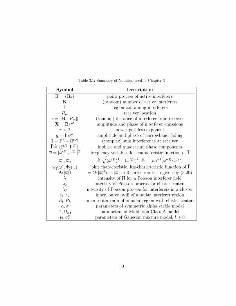
Table 3.1: Summary of Notation used in Chapter 3
Symbol Description
Π = Ri point process of active interferersK (random) number of active interferersΓ region containing interferersRm receiver location
r = ‖R−Rm‖ (random) distance of interferer from receiverX = Bejφ amplitude and phase of interferer emissionsγ > 2 power pathloss exponent
g = hejθ amplitude and phase of narrowband fadingI = I(I)+jI(Q) (complex) sum interference at receiver
I , I(I), I(Q) inphase and quadrature phase componentsω = [ω(I), ω(Q)]T frequency variables for characteristic function of I
|ω|, ωφ ,√
(ω(I))2
+ (ω(Q))2, , − tan−1(ω(Q)/ω(I))
ΦI(ω),ΨI(ω) joint characteristic, log-characteristic function of IΛ(|ω|) = O(|ω|4) as |ω| → 0 correction term given by (3.20)λ intensity of Π for a Poisson interferer fieldλc intensity of Poisson process for cluster centersλf intensity of Poisson process for interferers in a clusterrl, rh inner, outer radii of annular interferer regionRl, Rh inner, outer radii of annular region with cluster centersα, σ parameters of symmetric alpha stable modelA,Ω2A parameters of Middleton Class A modelpl, σ
2l parameters of Gaussian mixture model, l ≥ 0
50

Π = R1,R2, · · · over the space Γ, where Ri are the random locations of the
interferers. This model is sufficient to capture both the emerging interferers,
whose contributions arrive at the receiver for the first time at the time instant
n, and interferers that first emerged at some prior sampling time instant m < n
but are still active until the sample time n [72].
The baseband model for the sum interference I at any time instant can
then be represented as
I =K∑i=1
r− γ
2i giXi (3.1)
where K is the random number of active interferers at that time instant, i is the
interferer index, ri = ‖Ri−Rm‖ are the random distances of active interferers
from the receiver, γ is the power pathloss exponent, gi is the independent
and identically distributed (i.i.d.) random fast fading experienced by each
interferer emission, and Xi are the random interferer emissions.
All potential interferers are assumed to have i.i.d. symmetric narrow-
band emissions of the form [12]
Xi = Biejφi = Bi cos(φi) + jBi sin(φi) (3.2)
where Bi is the i.i.d. envelope, and φi is the i.i.d. random phase of the emis-
sions. Further, emerging times of the interferers are assumed to be uniformly
distributed between the sampling times at the receiver. Thus the phase φi
of the emissions at the sampling instants can be assumed to be uniformly
distributed on [0, 2π]. The assumption of i.i.d. emissions is valid for wire-
less communication networks without power control and may not be true for
51

modeling interference from diverse types of interferers with unequal transmit
power (e.g. base stations and mobile users).
The fast fading experienced by the interferer emissions is also assumed
to be narrowband of the form
gi = hiejθi (3.3)
where hi is the random amplitude scaling and θi is the random phase variation
due to fading. The in-phase and quadrature-phase components of the emis-
sions are assumed to experience uncorrelated fading and thus θi is uniformly
distributed on [0, 2π]. The sum interference can be expressed as
I =K∑i=1
r− γ
2i hiBi cos(φi+θi) + j
K∑i=1
r− γ
2i hiBi sin(φi+θi) (3.4)
3.3 Co-Channel Interference in a Poisson Field of In-terferers
Consider a scenario, as shown in Fig. 3.1, in which the spatial point
process Π in (3.1) is a homogeneous spatial Poisson point process with intensity
λ and the interferers are distributed over the space Γ(rl, rh). The parametric
interference space is defined as
Γ(rl, rh) =x ∈ R2 : rl ≤ ‖x‖ ≤ rh
. (3.5)
From (3.4), the joint characteristic function of the in-phase and quadrature-
phase components of the sum interference I = I(I) + jI(Q) can be expressed
52

Figure 3.1: Interference space and receiver location for different network topologies in a fieldof Poisson distributed interferers categorized by the region containing the interferers.
as
ΦI(I),I(Q)(ω(I), ω(Q))
= EI(I),I(Q)
ejω
(I)I(I)+jω(Q)I(Q)
(3.6)
= Eej∑Ki=1 r
− γ2i hiBi(ω(I) cos(φi+θi)+ω
(Q) sin(φi+θi))
(3.7)
= Eej|ω|
∑Ki=1 r
− γ2i hiBi cos(φi+θi+ωφ)
(3.8)
=∞∑k=0
Eej|ω|
∑ki=1 r
− γ2i hiBi cos(φi+θi+ωφ)
∣∣k in Γ(rl, rh)
P (k in Γ(rl, rh)) (3.9)
where ω = [ω(I), ω(Q)]T , |ω| =
√(ω(I))
2+ (ω(Q))
2, and ωφ = − tan−1
(ω(Q)
ω(I)
).
The expectation in (3.9) is with respect to the set of random variables
ri,hi,Bi,φi,θi.
Conditioned on the number of interferers present in the space Γ(rl, rh),
the interferer locations are mutually independent and uniformly distributed
53

across this space [125]. Henceforth, the conditioning on the number of in-
terferers is removed from the expectation by noting that the interferers are
uniformly distributed over Γ(rl, rh). Further, in the absence of power con-
trol, the interferer emissions can be assumed to be i.i.d.. The characteristic
function can then be expressed as
ΦY(ω) =∞∑k=0
[Eej|ω|r
− γ2 hB cos(φ+θ+ωφ)]k [λπ (r2
h − r2l )]
ke−λπ(r
2h−r
2l )
k!(3.10)
= eλπ(r2
h−r2l )(E
ej|ω|r−
γ2 hB cos(φ+θ+ωφ)
−1
)(3.11)
where Y is the set I(I), I(Q). By taking the logarithm of ΦY(ω), the log-
characteristic function is
ψY(ω) , log ΦY(ω) = λπ(r2h − r2
l
) (Eej|ω|r
− γ2 hB cos(φ+θ+ωφ)− 1). (3.12)
By using the identity
eja cos(φ) =∞∑k=0
jkεkJk(a) cos(kφ) (3.13)
where ε0 = 1, εk = 2 for k ≥ 1, and Jk(·) denotes the Bessel function of order
k, the log-characteristic function can be expressed as
ψY(ω)=λπ(r2h−r2
l
)(E
∞∑k=0
jkεkJk
(|ω|r−
γ2 hB
)cos (k(φ+ θ + ωφ))
−1
).
(3.14)
Since φ and θ are uniformly distributed on [0, 2π], Eφ,θ cos (k(φ+ θ + ωφ)) =
0 for k ≥ 1, and (3.14) reduces to
ψY(ω) = λπ(r2h − r2
l
) (Er,h,B
J0
(|ω|r−
γ2 hB
)− 1). (3.15)
54

The log-characteristic function derived in (3.15) holds in general for narrow-
band interferers distributed over the parametric space Γ(rl, rh), governed by
the parameters rh and rl and the receiver location Rm. The receiver loca-
tion Rm affects the expectation in (3.15). The following three cases are now
considered and the log-characteristic function is further simplified.
3.3.1 Case I: Interferers distributed over the entire plane (rl =0, rh →∞)
Consider a wireless network, as shown in Fig. 3.1, where the interfering
sources are distributed according to a spatial Poisson point process over the
entire plane. Note that ‖Rm‖ can be assumed to be zero without any loss in
generality of the result. This scenario corresponds to a decentralized network
in which nodes do not employ any contention-based MAC protocol, and has
been widely studied [63, 70–72, 108, 122, 123]. Lets consider the interference
space Γ(0, rh) and take the limit on the log-characteristic function as rh →∞
[63, 70]. Recall that the expectation in (3.15) is conditioned such that the
interferer locations are uniformly distributed over Γ(rl, rh). The distance of
each interferer from the receiver thus follows the distribution
fr|K(r|K) =
2rr2h
if 0 ≤ r ≤ rh,
0 otherwise.
Expanding the expectation in (3.15) gives
ψY(ω) = limrh→∞
λπr2h
rh∫0
Eh,B
J0
(|ω|r−
γ2 hB
) 2r
r2h
dr − 1
. (3.16)
55

Integrating the above by parts, noting that limrh→∞
Eh,B
r2h
(J0
(|ω|r−
γ2
h hB)−1)
= 0 for γ > 2, and ddxJ0(x) = −J1(x), gives
ψY(ω) = −|ω|4γ λπEh,B
h
4γB
4γ
∞∫0
J1(x)
x4γ
dx. (3.17)
Equation (3.17) is the log-characteristic function of a two-dimensional isotropic
symmetric alpha stable distribution centered at zero such that
ψI(I),I(Q)(ω(I), ω(Q)) = −σ∣∣∣∣√(ω(I))
2+ (ω(Q))
2
∣∣∣∣α (3.18)
where α = 4γ
is the characteristic exponent, and σ = λπEh,B hαBα∞∫0
J1(x)xα
dx
is the dispersion parameter of the symmetric alpha stable distribution [125].
Here, 0 < α < 2 and σ > 0. Hence, the sum interference in a Poisson field of
interferers distributed over the entire plane follows a symmetric alpha stable
distribution.
3.3.2 Case II: Interferers distributed over a finite-area annular re-gion (0 ≤ rl < rh <∞, Rm /∈ Γ(rl, rh))
Consider a wireless network, as shown in Fig. 3.1, where the interferers
are distributed over a finite-area annular region. When rl > 0 and ‖Rm‖ < rl,
this corresponds to a scenario where all the interferers are outside a guard
zone around the receiver and within a maximum distance (rh < ∞) beyond
which they do not generate significant interference. When ‖Rm‖ > rh, this
corresponds to a scenario where the interferers are distributed over a finite-
area circular or annular region with the receiver exterior to this region. The
56

former scenario is applicable for wireless networks with contention-based or
scheduling-based MAC protocols creating a guard zone around the receiver
(e.g. cellular networks with reuse factor of one and ad hoc networks with guard
zones [60]). The latter scenario is useful in characterizing the interference from
a hotspot (e.g. interferers localized in space around a cafe) and in cellular
networks with reuse factor greater than one. In cellular networks with reuse
factor greater than one, the interferers are distributed within a regular pattern
of isolated cell sites and the sum interference is thus a sum of the interference
from these isolated finite-area cell sites.
In [12], Middleton proposed an approximation of the log-characteristic
function for |ω| in the neighborhood of zero. From Fourier analysis, the behav-
ior of the characteristic function for |ω| in the neighborhood of zero governs
the tail probability of the random envelope. The proposed approximation is
based on the following identity [12]:
Er,h,B
J0
(|ω|r−
γ2 hB
)= e−
|ω|2Er,h,Br−γh2B24 (1 + Λ(|ω|)) (3.19)
where Λ(|ω|)) indicates a correction term with the lowest exponent in |ω| of
four and is given by
Λ(|ω|)) =∞∑k=2
(EZ Z)k |ω|2k
22kk!EZ
1F1
(−k; 1;
Z
EZ Z
)(3.20)
where the random variable Z = r−γh2B2, and 1F1 (a; b;x) is the confluent
hypergeometric function of the first kind, such that Λ(|ω|) = O(|ω|4) as |ω| →
0.
57

Using this identity, and approximating Λ (|ω|) 1 for |ω| in the neigh-
borhood of zero, the log-characteristic function in (3.15) can be expressed as
ψY(ω) ≈ λπ(r2h − r2
l
)(e−|ω|2Er,h,Br−γh2B2
4 − 1
). (3.21)
Equation (3.21) is the log-characteristic function of a Middleton Class A dis-
tribution such that
ψI(I),I(Q)(ω(I), ω(Q)) = A
(e−
((ω(I))
2+(ω(Q))
2)
Ω2A
2A − 1
)(3.22)
where A = λπ (r2h − r2
l ) is the overlap index that indicates the amount of
impulsiveness of the interference, and Ω2A =A×Er,h,Br−γh2B2
2is the mean
intensity of the interference [13]. Hence, the co-channel interference from a field
of Poisson distributed interferers over the finite-area space Γ(rl, rh) with Rm /∈
Γ(rl, rh) follows the Middleton Class A distribution. It should be emphasized
that the correspondence to the Middleton Class A distribution is particularly
valid for modeling the tail probabilities.
The approximation in (3.19) and the subsequent interference model
in (3.22) is valid for Rm /∈ Γ(rl, rh), since Ω2A → ∞ as ‖Rm‖ → rl or as
‖Rm‖ → rh. This is unlike Case I in Section 3.3.1 where the interference was
modeled for rl = 0. This is the key difference between the symmetric alpha
stable and Middleton Class A models for interference.
Next, I quantify the range of the system model parameters over which
the Middleton Class A model provides an accurate approximation to the co-
channel interference in this scenario. From (3.19), a first-order measure of the
58

accuracy of the approximation can be expressed by comparing the coefficient of
|ω|4 term in e−|ω|2Er,h,Br−γh2B2
4 against the coefficient of |ω|4 in the correction
term Λ(|ω|). Using the fact that
1F1 (−2; 1;x) =1
2(x2 − 4x+ 2), (3.23)
the coefficient of |ω|4 in the correction term (i.e., c4) can be expressed as
c4 =EZ Z2 − 2 [EZ Z]2
128. (3.24)
Thus, the Middleton Class A model provides a good approximation when the
system parameters, such as rh, rl, Rm, and γ, satisfy∣∣∣∣∣EZ Z2 − 2 [EZ Z]2
128
∣∣∣∣∣ [EZ Z]2
32(3.25)
⇒
∣∣∣∣∣ Er,h,B r−2γh4B44× [Er,h,B r−γh2B2]2
− 1
2
∣∣∣∣∣ 1. (3.26)
To provide some intuition about the above result, for a non-random h and B,
the condition is satisfied when ‖Rm‖ rl and rlrh
is greater than a fraction
that depends on γ and Rm, or when ‖Rm‖ rh. The conditions ‖Rm‖ rl
and ‖Rm‖ rh ensure that the interferers are not close to the receiver and
a lower bound on rlrh
ensures that rh is not very large compared to rl when
‖Rm‖ < rl.
3.3.3 Case III: Interferers distributed over infinite-area annular re-gion with guard zone (rl > 0, rh →∞, and ‖Rm‖ < rl)
Consider a wireless network, as shown in Fig. 3.1, where the interfering
sources are distributed according to a spatial Poisson point process on the
59

entire plane, except within a guard zone around the receiver. The applicability
of Case II for guard zone scenarios was limited to finite-area fields and does
provide a good approximation for a wide range of system parameters. In
this subsection, the interference region is allowed to have infinite area and is
thereby more applicable to large random wireless networks with guard zones
[60]. Lets consider the interference space Γ(rl, rh) and take the limit on the log-
characteristic function as rh → ∞. Conditioned on the number of interferers
in Γ(rl, rh), the interferer locations are mutually independent and uniformly
distributed in the space Γ(rl, rh). Thus as rh → ∞, with high probability,
the distance of an interferer from receiver located at Rm can be approximated
as r = ‖R − Rm‖ ≈ ‖R‖, particularly for ‖Rm‖ rl. The distance of each
interferer from the receiver thus follows the distribution
fr|K(r|K) =
2r
r2h−r
2l
if rl ≤ r ≤ rh,
0 otherwise.
Expanding the expectation in (3.15) gives
ψY(ω) = limrh→∞
λπ(r2h − r2
l )
rh∫rl
Eh,B
J0
(|ω|r−
γ2 hB
) 2r
r2h − r2
l
dr − 1
.
(3.27)
Integrating the above by parts, reordering terms, and noting that
limrh→∞
λπr2h
(Eh,B
J0
(|ω|r−
γ2
h hB)−1)
= 0 for γ > 2, gives
ψY(ω) = −λπr2l
(Eh,B
J0
(|ω|r−
γ2
l hB)−1)
− limrh→∞
λπ
rh∫rl
∂
∂r
(Eh,B
J0
(|ω|r−
γ2 hB
))r2dr. (3.28)
60

Invoking the identity (3.19), and approximating Λ (|ω|) 1 for |ω| in the
neighborhood of zero, the log-characteristic function can be expressed as
ψY(ω) ≈ − λπr2l
(e−|ω|2r−γ
lEh,Bh2B2
4 − 1
)
− limrh→∞
λπ
∫ rh
rl
∂
∂r
(e−|ω|2r−γEh,Bh2B2
4
)r2dr. (3.29)
Note that unlike (3.19), the approximation in (3.29) involves a non-random r.
Using Taylor series expansion of ex, the log-characteristic function reduces to
ψY(ω) = λπr2l
[∞∑k=1
(−1)k|ω|2k
4kk!
(Eh2B2
)kr−γkl
2
kγ − 2
](3.30)
valid for γ > 2. The 2kγ−2
multiplicative factor inside the summation prevents
the log-characteristic function to be expressed in closed form. I thus approxi-
mate the function 2kγ−2
as ηeβk for k ≥ 1. The parameters η and β are chosen
to minimize the weighted mean squared error (WMSE)
η, β = arg minη,β
∞∑k=1
(2
kγ − 2− ηeβk
)2
u(k) (3.31)
where u(k) are the weights. The weights should be chosen such that penalty of
error is large when k is small, since it affects the coefficients of terms with lower
order exponents of |ω|. Equation (3.31) is an unconstrained nonlinear opti-
mization problem and can be solved efficiently using numerical techniques such
as quasi-Newton methods [1]. Quasi-Newton methods have superlinear con-
vergence and require O(ln(| ln(ε)|)) number of iterations and O(d2 ln(| ln(ε)|))
algebraic computational effort, where d is the dimensionality of the problem
and ε is the maximum permissible error tolerance in the result. Table 3.2
61

Table 3.2: Values for η, β and the associated weighted mean squared error (WMSE),obtained by solving (3.31), for different values of the power pathloss exponent (γ) and usingthe weighting function u(k) = e−k. Solution to (3.31) was obtained by using the fminuncfunction in MATLAB, which uses the BFGS quasi-Newton method [1].
γ η, β WMSE
2.5 22.818,−1.741 4.32× 10⁻³
3.0 7.484,−1.321 1.84× 10⁻³
3.5 4.132,−1.132 9.81× 10⁻⁴
4.0 2.781,−1.025 5.96× 10⁻⁴
4.5 2.073,−0.954 3.96× 10⁻⁴
5.0 1.645,−0.905 2.80× 10⁻⁴
lists the values for η, β and the associated WMSE for certain values of γ,
using the weights u(k) = e−k. By approximating 2kγ−2
as ηeβk for k ≥ 1, the
log-characteristic exponent can be expressed as
ψY(ω) ≈ λπr2l η
(e−|ω|2r−γ
leβEh,Bh2B2
4 − 1
). (3.32)
Equation (3.32) is the log-characteristic function of a Middleton Class A dis-
tribution such that
ψI(I),I(Q)(ω(I), ω(Q)) = A
(e−
((ω(I))
2+(ω(Q))
2)
Ω2A
2A − 1
)(3.33)
where A = λπr2l η is the overlap index that indicates the impulsiveness of
the interference, and Ω2A =A×r−γl eβEh,Bh2B2
2is the mean intensity of the
interference [13].
The functional form of ηeβk to approximate 2kγ−2
for k ≥ 1 was chosen
since, a) it provides a good approximation and enables the log-characteristic
function to be expressed in closed form, and b) provides two parameters η, β
62

such that η affects only the impulsive index A, while β affects only the vari-
ance σ2m = m
AΩ2A of individual components of the Gaussian mixture form of
Middleton Class A model.
Similar to Case II, a first-order measure of accuracy of the approxima-
tion can be expressed by comparing the coefficient of |ω|4 term in the true
log-characteristic function (3.28) against the the coefficient of |ω|4 term in
the approximated log-characteristic function (3.32). The two approximations
involved are using ηeβk to approximate the function 2kγ−2
for k ≥ 1, and ap-
proximating Λ (|ω|) 1 for |ω| close to zero. Note that the lowest order
term affected by the former approximation is the coefficient of |ω|2 term. The
approximation error is assumed to be negligible due to the optimization in
(3.31). Using (3.19) and (3.20), the coefficient of |ω|4 term in the true log-
characteristic function (3.32) is
λπr−2γ+2l
(E Z2+ 2 [E Z]2
128
)(2
2γ − 2
)where Z = h2B2. Comparing with the coefficient of |ω|4 term in (3.32), the
Middleton Class A distribution provides a good approximation to co-channel
interference statistics in this scenario when∣∣∣∣∣(
[E Z]2
64
)(2
2γ − 2− 2ηe2β
)+
(E Z2
128
)(2
2γ − 2
)∣∣∣∣∣∣∣∣∣∣ [E Z]232
ηe2β
∣∣∣∣∣ .(3.34)
Note that if ηe2β = 22γ−2
, then the above condition is same as the one obtained
for Case II in (3.25), with the exception that Z = h2B2 in this case. The above
63

Figure 3.2: Interference space and receiver location for different network topologies in a fieldof Poisson-Poisson cluster distributed interferers categorized by the region containing thecluster centers.
condition is independent of the parameter rl that governs the interference space
and is valid when the variance of h2B2 is low when compared to [Eh2B2]2.
The above condition does not capture the error due to the approximation
r = ‖R − Rm‖ ≈ R, which is true with high probability in this scenario and
is particularly valid for ‖Rm‖ rl.
3.4 Co-Channel Interference in a Poisson-Poisson Clus-ter Field of Interferers
Consider a scenario, as shown in Fig. 3.2, where the interferers are clus-
tered in space. The center of the clusters are assumed to distributed according
to a spatial Poisson point process Πc with intensity λc over the space Γ(Rl, Rh).
For each cluster center Rc ∈ Πc, interferers are assumed to be distributed ac-
cording to an independent spatial Poisson process Πc,f with intensity λf over
64

the space Γ(rl, rh) around the center Rc. The point process Π in (3.1) is then
a homogeneous spatial Poisson-Poisson cluster process such that
Π =⋃
Rc∈Πc
⋃Rc,f∈Πc,f
Rc + Rc,f . (3.35)
Note that the cluster centers are themselves not included. The parametric
interference space Γ(·, ·) is defined in (3.5). When rl = 0, Π is a Matern
cluster process [129].
The joint characteristic function of the in-phase and quadrature-phase
components of the sum interference I = I(I) + jI(Q) can be expressed as
ΦI(I),I(Q)(ω(I), ω(Q))
= EI(I),I(Q)
ejω
(I)I(I)+jω(Q)I(Q)
(3.36)
= Eej|ω|
∑Kci=1
∑Kc,fm=1 r
− γ2i,mhi,mBi,m cos(φi,m+θi,m+ωφ)
(3.37)
=∞∑kc=0
Eej|ω|
∑kci=1
∑Kc,fm=1 r
− γ2i,mhi,mBi,m cos(φi,m+θi,m+ωφ)
∣∣kc in Γ(Rl, Rh)
× P (kc in Γ(Rl, Rh)) (3.38)
where Kc is the random number of active clusters, Kc,f is the random number
of active interferers per cluster, ω = [ω(I), ω(Q)]T , |ω| =
√(ω(I))
2+ (ω(Q))
2,
and ωφ = − tan−1(ω(Q)
ω(I)
). The expectation in (3.38) is with respect to the
set of random variablesKc,f , ri,m,hi,m,Bi,m,φi,m,θi,m
. The indexing (·)i,m
denotes the mth active interferer in the ith cluster.
Conditioned on the number of clusters present in the space Γ(Rl, Rh),
location of the cluster centers (Rc) are mutually independent and uniformly
65

distributed over this space [125]. Further, in the absence of power control, the
sum interference from each cluster can be assumed to be i.i.d., such that
ΦY(ω) =∞∑kc=0
[Eej|ω|
∑Kc,fm=0 r
− γ2m hmBm cos(φm+θm+ωφ)
]kc× [λcπ (R2
h −R2l )]
kc e−λcπ(R2h−R
2l )
kc!(3.39)
= eAc
(E
ej|ω|
∑Kc,fm=0 r
− γ2m hmBm cos(φm+θm+ωφ)
−1
)(3.40)
where Y is the set I(I), I(Q), and Ac = λcπ (R2h −R2
l ). The expectation in
(3.40) is with respect to the set of random variables Rc,Kc,f ,Rc,m,hm,Bm,
φm,θm. By taking the logarithm of ΦY(ω), the log-characteristic function is
ψY(ω) = Ac
(Eej|ω|
∑Kc,fm=0 r
− γ2m hmBm cos(φm+θm+ωφ)
− 1
). (3.41)
The above equation can be expressed in the form
ψY(ω) = Ac(ERc
EIc,f
ej|ω|Ic,f
− 1)
(3.42)
where Ic,f is the sum interference from an interferer cluster and is a function
of the set of random variables Kc,f ,Rc,m,hm,Bm,φm,θm, similar to (3.8).
Thus Ic,f is the sum interference from a field of Poisson distributed interferers
over the interference space Γ(rl, rh) around the cluster center Rc. Using (3.15),
the log-characteristic function can then be expressed as
ψY(ω) = Ac
[ERc
eAf
(ERc,f ,h,B
J0
(|ω|r−
γ2 hB
)−1)− 1
](3.43)
where Af = λfπ (r2h − r2
l ), r = ‖Rc + Rc,f −Rm‖, Rc is uniformly distributed
in Γ(Rl, Rh), and Rc,f is uniformly distributed in Γ(rl, rh).
66

The log-characteristic function derived in (3.43) holds in general for
a Poisson-Poisson clustered field of narrowband interferers, where the cluster
centers are distributed over the parametric space Γ(Rl, Rh) and the interferers
are distributed over the parametric space Γ(rl, rh) around each cluster center.
The receiver location Rm affects the inner expectation in (3.43). I now consider
the same three cases, categorized by the region containing the cluster centers,
and further simplify the log-characteristic function.
3.4.1 Case I: Cluster centers distributed over the entire plane (Rl =0, Rh →∞)
Consider a wireless network scenario, as shown in Fig. 3.2, where the
center of interferer clusters are distributed according to a homogeneous spatial
Poisson point process over the entire plane. Similar to Case I for a Poisson field
of interferers, ‖Rm‖ can be assumed to be zero without any loss in generality
of the result. Conditioned on the number of clusters in Γ(0, Rh), the distance
of each cluster center from the origin follows the distribution
fRc|Kc(Rc|Kc) =
2RcR2h
if 0 ≤ Rc ≤ Rh,
0 otherwise.
Thus as Rh → ∞, with high probability, the distance of an interferer from
the receiver can be approximated as r = ‖Rc + Rc,f‖ ≈ ‖Rc‖. Expanding the
expectation over Rc in (3.43) and using the Taylor series expansion of ex gives
ψY(ω) = limRh→∞
Ac
Rh∫0
eAf
(EJ0
(|ω|R
− γ2c hB
)−1
)2Rc
R2h
dRc−1
67

= e−Af∞∑k=0
Akfk!
limRh→∞
Ac
Rh∫0
(EJ0
(|ω|R−
γ2
c hB))k 2Rc
R2h
dRc − 1
= e−Af
∞∑k=0
Akfk!
Υ (3.44)
where
Υ = limRh→∞
Ac
Rh∫0
(EJ0
(|ω|R−
γ2
c hB))k 2Rc
R2h
dRc − 1
. (3.45)
Integrating the above by parts, reordering terms, and noting that
limRh→∞
Ac
[(EJ0
(|ω|R−
γ2
h hB))k
− 1
]= 0 for γ > 2, gives
Υ = limRh→∞
−λcπ∫ Rh
0
∂
∂Rc
[(EJ0
(|ω|R−
γ2
c hB))k]
R2c dRc. (3.46)
Invoking the identity (3.19), and approximating Λ(|ω|)) 1 for |ω| close to
zero, gives[EJ0
(|ω|R−
γ2
c hB)]k
= e−|ω|2kR−γc Eh2B2
4 (1 + Λ(|ω|))k (3.47)
≈ EJ0
(|ω|√kR− γ
2c hB
). (3.48)
Substituting (3.48) in (3.46), and noting that ddxJ0(x) = −J1(x), gives
Υ = −|ω|4γ λcπ
(√k) 4γ Eh,B
h
4γB
4γ
∞∫0
J1(x)
x4γ
dx. (3.49)
Using (3.49), the log-characteristic function in (3.44) reduces to
ψY(ω) = −|ω|4γ
(λcπEh,B
h
4γB
4γ
∫ ∞0
J1(x)
x4γ
dx
) ∞∑k=0
e−AfAkf
(√k) 4γ
k!
.(3.50)
68

Equation (3.50) is the log-characteristic function of a two-dimensional isotropic
symmetric alpha stable distribution centered at zero such that
ψI(I),I(Q)(ω(I), ω(Q)) = −σ∣∣∣∣√(ω(I))
2+ (ω(Q))
2
∣∣∣∣α (3.51)
where α = 4γ
is the characteristic exponent (0 < α < 2), and σ =[(λcπ
Eh,B hαBα∫∞
0J1(x)xα
dx)∑∞
k=0
e−AfAkf(
√k)α
k!
]is the dispersion parameter (σ >
0) of the symmetric alpha stable distribution [125]. Hence, when the center
of interferer clusters are distributed according to a spatial Poisson process on
the entire plane, the co-channel interference follows a symmetric alpha stable
distribution. Note that unlike Case I for a Poisson field of interferers, the sym-
metric alpha stable distribution is not an exact model due to approximation
in (3.48), but accurately models the tail probability of the interference.
3.4.2 Case II: Cluster centers distributed over finite-area annularregion (0 ≤ Rl < Rh <∞, and Rm /∈ Γ(Rl − rh, Rh + rh))
Consider a wireless network scenario, as shown in Fig. 3.2, where the
cluster centers are distributed over a finite-area annular region. The receiver
location is such that it does not belong to the space of active interferers (Rm /∈
Γ(Rl − rh, Rh + rh)). Similar to Case II for a Poisson field of interferers, this
scenario is useful in characterizing interference from a finite-area annular field
when the receiver is located interior to the region with a guard zone (when
‖Rm‖ < Rl − rh) or at a point exterior to the region (when ‖Rm‖ > Rh + rh).
Using the identity (3.19), the log-characteristic function in (3.43) can
69

be expressed as
ψY(ω)=Ac
[ERc
exp
(Af
(e−|ω|2ERc,f ,h,Br−γh2B2
4 (1+Λ(|ω|))−1
))−1
](3.52)
where Λ(|ω|) is the correction term given by (3.20). For notational simplicity,
let F = ERc,f ,h,B r−γh2B2. F is then a function of the random variable Rc.
Approximating Λ(|ω|)) 1 for |ω| in the neighborhood of zero, and using the
Taylor series expansion of ex, the log-characteristic function reduces to
ψY(ω) ≈ Ac
[ERc
e−Af
∞∑k=0
Akfk!e−k|ω|2F
4
− 1
](3.53)
= Ac
[e−Af
∞∑l=0
(−1)l|ω|2lERc
Fl
4ll!
∞∑k=0
Akfkl
k!− 1
]. (3.54)
To express the log-characteristic function in closed form, I approximate ERc
Fl
≈ (ERc F)l. This approximation holds with equality for l = 0, 1 and hence
does not affect the coefficient of |ω|2 term. The coefficient of the lowest
order term affected by this approximation is the |ω|4 term. Thus the log-
characteristic function is not severely affected by this approximation for |ω|
in the neighborhood of zero, which is desired for accurately modeling the tail
probability, and can be expressed as
ψY(ω) ≈ Ac
[exp
(Af
(e−|ω|2ERc
F4 − 1
))− 1
]. (3.55)
Using the log-characteristic function, and using the Taylor series expansion
from ex, the characteristic function can be expressed as
ΦY(ω) = e−Ac∞∑l=0
Alfl!
(∞∑k=0
Akckle−kAf
k!
)e−l|ω|2ERc
F4 . (3.56)
70

Equation (3.56) is the characteristic function of a two-dimensional isotropic
Gaussian mixture model such that
ΦI(I),I(Q)(ω(I), ω(Q)) =∞∑l=0
ple−((ω(I))
2+(ω(Q))
2)σ2l
2 (3.57)
where pl =e−AcAlf
l!
(∑∞k=0
Akckle−kAf
k!
)are the mixture probabilities, and σ2
l =
l×ERc,Rc,f ,h,Br−γh2B22
are the variance of the individual Gaussian components,
for l ≥ 0.
The two approximations involved in expressing the true log-characteristic
function (3.52) as (3.55) are approximating Λ (|ω|) 1 for |ω| in the neigh-
borhood of zero, and expressing ERc
Fl
as (ERc F)l. Using (3.20), the
coefficient of |ω|4 term in the true log-characteristic function (3.52) can be
expressed as
Ace−Af
[ERc F2
32
∞∑k=0
k2Akfk!
+ ERc c4∞∑k=0
kAkfk!
]
where c4=ERc,f ,h,Br−2γh4B4−2
(ERc,f ,h,Br−γh2B2
)2
128, and F=ERc,f ,h,B r−γh2B2.
Comparing with the coefficient of the |ω|4 term in the approximated log-
characteristic function (3.55), the Gaussian mixture distribution provides a
good approximation to the interference statistics in this scenario when∣∣∣∣∣V ar(F)
32
∞∑k=0
k2Akfk!
+ ERc c4∞∑k=0
kAkfk!
∣∣∣∣∣∣∣∣∣∣(ERc F)
2
32
∞∑k=0
k2Akfk!
∣∣∣∣∣ (3.58)
where V ar(F) = ERc F2−(ERc F)2. Intuitively, the above condition is sat-
isfied when the interferers are not close to the receiver (i.e., ‖Rm‖ Rl − rh
or ‖Rm‖ Rh + rh) and Rh is not very high compared to Rl when ‖Rm‖ <
Rl − rh.
71

3.4.3 Case III: Cluster centers distributed over infinite-area annu-lar region with guard zone (Rl > 0, Rh →∞, and ‖Rm‖ < Rl−rh)
Consider a wireless network, as shown in Fig. 3.2, where the center of
interferer clusters are distributed according to a homogeneous spatial Poisson
point process over the entire plane, except within a guard zone around the
receiver. Analogous to Case III for a Poisson field of interferers, the distance
of each cluster center from the origin follows the distribution
fRc|Kc(Rc|Kc) =
2Rc
R2h−R
2l
if Rl ≤ Rc ≤ Rh,
0 otherwise.
Thus as Rh → ∞, with high probability, the distance of an interferer from
receiver located at Rm can be approximated as r = ‖Rc + Rc,f − Rm‖ ≈
‖Rc‖, particularly for Rm Rl − rh. Analogous to Case I, on expanding the
expectation over Rc in (3.43) and using the Taylor series expansion for ex gives
ψY(ω) = limRh→∞
Ac
Rh∫Rl
eAf
(EJ0
(|ω|R
− γ2c hB
)−1
)2Rc
R2h −R2
l
dRc − 1
(3.59)
= e−Af∞∑k=0
Akfk!
Υ (3.60)
where
Υ = limRh→∞
Ac
Rh∫Rl
(EJ0
(|ω|R−
γ2
c hB))k 2Rc
R2h −R2
l
dRc − 1
. (3.61)
Integrating the above by parts, reordering terms, and noting that
limRh→∞
λcπR2h
[(EJ0
(|ω|R−
γ2
h hB))k −1
]= 0 for γ > 2, gives
Υ = −λcπR2l
((Eh,B
J0
(|ω|R−
γ2
l hB))k
− 1
)−
72

limRh→∞
λcπ
Rh∫Rl
∂
∂Rc
[(Eh,B
J0
(|ω|R−
γ2
c hB))k]
R2c dRc. (3.62)
Invoking the identity (3.19), approximating Λ (|ω|) 1 for |ω| in the neigh-
borhood of zero, and using the Taylor series expansion of ex, gives
Υ ≈ λcπR2l
[∞∑m=1
(−1)m|ω|2mkm
4mm!
(Eh2B2
)mR−γml
2
γm− 2
]. (3.63)
Similar to Case III for Poisson field of interferers, the 2γm−2
multiplica-
tive factor inside the summation prevents Υ, and hence the log-characteristic
function, to be expressed in closed form. I thus approximate the function
2γm−2
as ηeβm for m ≥ 1, where η, β are chosen to minimize a weighted
mean squared error (WMSE) criterion as discussed in Section 3.3.3. Using
this approximation, (3.63) reduces to
Υ ≈ λcπR2l η
(e−l|ω|2R−γ
leβEh2B24 − 1
)(3.64)
Substituting the above equation in (3.60), the log-characteristic function can
be expressed as
ψY(ω) = λcπR2l η
[exp
(Af
(e−|ω|2R−γ
leβEh2B24 − 1
))− 1
]. (3.65)
Using the log-characteristic function, and the Taylor series expansion for ex,
the characteristic function can be expressed as
ΦY(ω) = e−λcπR2l η
∞∑l=0
[Alfl!
(∞∑k=0
(λcπR2l η)
kkle−kAf
k!
)e−l|ω|2R−γ
leβEh2B24
].
(3.66)
73

Equation (3.66) is the characteristic function of a two-dimensional isotropic
Gaussian mixture model such that
ΦI(I),I(Q)(ω(I), ω(Q)) =∞∑l=0
ple−((ω(I))
2+(ω(Q))
2)σ2l
2 (3.67)
where pl =e−λcπR
2l ηAlf
l!
(∑∞k=0
(λcπR2l η)
kkle−kAf
k!
)are the mixture probabilities,
and σ2l =
l×R−γl eβEh,Bh2B22
are the variance of the individual Gaussian com-
ponents, for l ≥ 0.
Using (3.62), (3.19), and (3.20), the coefficient of |ω|4 term in the true
log-characteristic function (3.60) can be expressed as
λcπR−2γ+2l e−Af
[(E Z)2
32
∞∑k=0
k2Akfk!
+ c4
∞∑k=0
kAkfk!
](2
2γ − 2
). (3.68)
where Z = h2B2 and c4 =EZ2−2(EZ)2
128. Comparing with the coefficient
of |ω|4 term in the approximated log-characteristic function (3.66), the Gaus-
sian mixture distribution provides a good approximation to the interference
statistics in this scenario when∣∣∣∣∣(E Z)2
32
(2
2γ − 2− ηe2β
) ∞∑k=0
k2Akfk!
+2c4
(2γ − 2)
∞∑k=0
kAkfk!
∣∣∣∣∣
∣∣∣∣∣(E Z)2
32ηe2β
∞∑k=0
k2Akfk!
∣∣∣∣∣ . (3.69)
Analogous to Case III for a Poisson field of interferers, the above condition
is independent of the parameter Rl that governs the interference space and is
satisfied when the variance of the random variable h2B2 is low when compared
to [Eh2B2]2. Note that the above condition does not capture the error due
74

to the approximation r = ‖Rc + Rc,f − Rm‖ ≈ Rc, which is true with high
probability and is particularly valid for ‖Rm‖ Rl − rh.
3.5 Summary and Discussion
Tables 3.3 and 3.4 summarize the key results derived in this chapter for
a field of Poisson and Poisson-Poisson cluster distributed interferers, respec-
tively. The following observations are made.
1. Narrowband emissions from interferers: The narrowband form of
the interfering emissions is truly attributed to the narrowband filtering
done at the receiver. Hence the interferer emissions can have a higher
bandwidth than the receiver, as long as the transients caused due to
interferer emissions at the receiver can be ignored [13]. From [13], the
analysis and results presented in this chapter are valid as long as the
duration of the interfering emissions (TI) is much greater than the recip-
rocal of the receiver bandwidth (∆fR), i.e., TI 1∆fR
.
2. Extensions for finite-area interference fields with arbitrary shape:
The finite-area cases are studied for Poisson and Poisson-Poisson clus-
tered field of interferers in Sections 3.3.2 and 3.4.2, respectively. For a
finite-area interference Γ with arbitrary shape, P k in Γ = λ|Γ|, where
|Γ| denotes the area of the space Γ in (3.9) and (3.38). The remaining
analysis does not change since the expectation over the random variable
r is not expanded for finite-area cases. Hence it can be readily shown
75

Table 3.3: Statistical-physical modeling of co-channel interference in a field of Poisson dis-tributed interferers categorized by the region containing the interferers.
Poisson field of Interferers
Wireless Sce-nario
Example WirelessNetwork
Statistical Model
Case I: EntirePlane(rl = 0, rh →∞)
Sensor or Ad hocnetworks
Symmetric Alpha StableParameters:α= 4
γ
σ=λπEh,B hαBα∞∫0
J1(x)xα
dx
Models exact statistics
Case II: Finite-areaAnnular Region(0 ≤ rl < rh <∞,andRm /∈ Γ (rl, rh))
a. Cellular networks(out-of-cellinterference)
b. Interference from ahotspot (e.g. cafe)
Middleton Class AParameters:A = λπ (r2
h − r2l )
Ω2A =A×Er,h,Br−γh2.B2
2
where r = ‖R−Rm‖.Models tail probabilitywhen (3.26) is met.
Case III:Infinite-area withGuard Zone(rl > 0, rh →∞,and ‖Rm‖ < rl)
a. Cellular networks(out-of-cellinterference)
b. Decentralizednetworks withcontention-basedMAC protocols
c. Dense WiFinetworks
Middleton Class AParameters:A = λπr2
l η
Ω2A =A×r−γl eβEh,Bh2.B2
2
where η, β are obtainedfrom (3.31).Models tail probabilitywhen (3.34) is met.
76

Table 3.4: Statistical-physical modeling of co-channel interference in a field of Poisson-Poisson cluster distributed interferers categorized by the region containing the cluster cen-ters.
Poisson-Poisson Cluster field of Interferers
Wireless Sce-nario
Example WirelessNetwork
Statistical Model
Case I: EntirePlane(Rl = 0, Rh →∞)
a. Two-tier femtocellnetworks(femtocellinterference)
b. Sensor or ad hocnetworks withgeographical orMAC inducedclustering
Symmetric Alpha StableParameters:α= 4
γ
σ=
[λcπEh,B hαBα
∞∫0
J1(x)xα
dx
]×∞∑k=0
e−AfAkf(
√k)α
k!
where Af = λfπ (r2h − r2
l ).Models tail probability.
Case II: Finite-areaAnnular Region(0≤Rl<Rh<∞,and Rm /∈Γ (Rl−rh, Rh+rh))
a. Cellular networks(out-of-cellinterference) withuser clustering
b. Interference fromregion withmultiple (random)hotspots(e.g. market place,university)
Gaussian Mixture ModelParameters:
pl =e−AcAlf
l!
(∞∑k=0
Akckle−kAf
k!
)σ2l =
l×ERc,Rc,f ,h,Br−γh2B22
where Ac = λcπ (R2h −R2
l ),Af = λfπ (r2
h − r2l ), and
r = ‖Rc + Rc,f −Rm‖.Models tail probability when(3.58) is met.
Case III:Infinite-area withGuard Zone(Rl > 0, Rh →∞,and‖Rm‖ < Rl − rh)
a. Two-tier femtocellnetworks(out-of-cellfemtocellinterference)
b. Cellular networks(out-of-cellinterference) withuser clustering
Gaussian Mixture ModelParameters:
pl=e−λcπR
2l ηAlf
l!
∞∑k=0
(λcπR2l η)
kkle−kAf
k!
σ2l =
l×R−γl eβEh,Bh2B22
where Af = λfπ (r2h − r2
l ),η, β are obtained from(3.31).Models tail probability when(3.69) is met.
77

that Middleton Class A and the Gaussian mixture models are still ap-
plicable for interference spaces with arbitrary shape using the following
changes in the parameters. The overlap index for Middleton Class A
is expressed more generally as A = λ|Γ| for finite-area field of Poisson
distributed interferers. For finite-area field of Poisson-Poisson cluster
distributed interferers, the parameters Af = λf |Γf | and Ac = λc|Γc|,
where Γc is the space in which the cluster centers are distributed and Γf
is the space in which the interferers are distributed around each cluster
center.
3.6 Simulation Results
Using the physical model discussed in Section 3.2, I apply Monte-Carlo
numerical techniques to simulate the co-channel interference observed at the
receiver in various wireless network environments based on (3.1). At each sam-
ple instant, the location of the active interferers is generated as a realization of
a spatial Poisson or Poisson-Poisson cluster point process. Parameter values
governing the interference space and the receiver location change according
to the wireless network model under consideration. It should be noted that
parameters denoting distance are are treated as dimensionless quantities as
this does not influence the statistics of the resultant interference.
System model parameters used in the numerical simulations are
γ = 4, h ∼ Rayleigh
(1√2
), λ = 10−4, λc = 10−4, λf = 10−3.
78

The amplitude of the interferer emissions, B, was chosen as a constant for a
particular wireless environment such that the tail probability, P(‖I‖ > y), at
an interference threshold of y = 7, is of the order of 10−4. The probability
distribution of co-channel interference is empirically estimated from 500000
time samples of the received interference using kernel smoothed density esti-
mators [130].
Accuracy of the statistical models is established by comparing the em-
pirical and interference model tail probabilities. I compare the asymptotic
decay rates of the tail probabilities given by
ρ (y) = − log (P(‖I‖ > y))
y(3.70)
where ρ(y) is the asymptotic decay rate at interference amplitude y. The decay
rate is the rate at which the tail probability asymptotically approaches zero.
The decay rates are a useful measure to compare the extreme value statis-
tics of different statistical models with respect to the empirically estimated
distribution.
Accuracy of fit of the statistical models is also quantified using the
Kullback-Leibler divergence (KLD) measure [131], where a KLD of zero indi-
cates an exact match of the densities. Lower KLD, however, does not imply
correspondence in tail probabilities since the KLD is the relative error between
two distribution functions over their entire support. Thus, even though a sta-
tistical model has a low KLD with respect to the empirical distribution, it may
be an inaccurate model for modeling extreme statistics.
79

4.5 5 5.5 6 6.5 70
0.5
1
1.5
2
2.5
3
3.5
4
Interference Amplitude
De
ca
y R
ate
Empirical
SAS
Figure 3.3: Decay rates for tail probabilities of simulated co-channel interference and thesymmetric alpha stable (SAS) model for Case I (rl = 0, rh =∞,B = 5) of Poisson field ofinterferers. The Middleton Class A and Gaussian models are not suitable in this scenarioas the mean intensity Ω2A →∞.
4.5 5 5.5 6 6.5 70
0.5
1
1.5
2
2.5
3
3.5
4
4.5
5
Interference Amplitude
De
ca
y R
ate
Empirical
SAS
MCA
Gaussian
Figure 3.4: Decay rates for tail probabilities of simulated co-channel interference and thesymmetric alpha stable (SAS), Middleton Class A (MCA), and Gaussian models for CaseII (rl = 20, rh = 40, ‖Rm‖ = 4,B = 1400) of Poisson field of interferers. MCA has the bestmatch to the empirical (simulated) co-channel interference.
80

4.5 5 5.5 6 6.5 70
0.5
1
1.5
2
2.5
3
3.5
4
4.5
Interference Amplitude
De
ca
y R
ate
Empirical
SAS
MCA
Gaussian
Figure 3.5: Decay rates for tail probabilities of simulated co-channel interference and thesymmetric alpha stable (SAS), Middleton Class A (MCA), and Gaussian models for CaseIII (rl = 30, rh = ∞, ‖Rm‖ = 4,B = 2200) of Poisson field of interferers. η, β =2.781,−1.025 for γ = 4 and u(k) = e−k from Table 3.2. MCA has the best match to theempirical (simulated) co-channel interference.
3.6.1 Co-channel interference in a Poisson field of interferers
Figs. 3.3, 3.4, and 3.5 show the decay rates of the empirical distribution
compared with the statistical models for Case I, Case II, and Case III (see
Fig. 3.1), respectively. In each scenario, the empirical distribution is compared
against the symmetric alpha stable and the Middleton Class A distribution
with appropriate parameters (see Table 3.3), and a Gaussian distribution with
equal variance.
For a Poisson field of interferers, the results demonstrate that the tail
probabilities of the co-channel interference in Case I are well modeled us-
ing a symmetric alpha distribution, while the Middleton Class A distribution
provides a good fit to the tail probabilities in Case II and Case III.
81

4.5 5 5.5 6 6.5 70
0.5
1
1.5
2
2.5
3
3.5
4
Interference Amplitude
De
ca
y R
ate
Empirical
SAS
Figure 3.6: Decay rates for tail probabilities of simulated co-channel interference and thesymmetric alpha stable (SAS) model for Case I (Rl = 0, Rh =∞, rl = 0, rh = 10,B = 100)of Poisson-Poisson cluster field of interferers. The Gaussian mixture and Gaussian modelsare not suitable in this scenario as the mean intensity Ω2A →∞.
4.5 5 5.5 6 6.5 70
0.5
1
1.5
2
2.5
3
3.5
4
Interference Amplitude
De
ca
y R
ate
Empirical
SAS
GMM
Gaussian
Figure 3.7: Decay rates for tail probabilities of simulated co-channel interference and thesymmetric alpha stable (SAS), Gaussian mixture (GMM), and Gaussian models for Case II(Rl = 40, Rh = 80, rl = 0, rh = 10, ‖Rm‖ = 4,B = 6000) of Poisson-Poisson cluster field ofinterferers. GMM has the best match to the empirical (simulated) co-channel interference.
82

4.5 5 5.5 6 6.5 70
0.5
1
1.5
2
2.5
3
3.5
4
Interference Amplitude
De
ca
y R
ate
Empirical
SAS
GMM
Gaussian
Figure 3.8: Decay rates for tail probabilities of simulated co-channel interference and thesymmetric alpha stable (SAS), Gaussian mixture (GMM), and Gaussian models for Case III(Rl = 30, Rh →∞, rl = 0, rh = 10, ‖Rm‖ = 4,B = 4000) of Poisson-Poisson cluster field ofinterferers. η, β = 2.781,−1.025 for γ = 4 and u(k) = e−k from Table 3.2. MCA hasthe best match to the empirical (simulated) co-channel interference.
3.6.2 Co-channel interference in a Poisson-Poisson cluster field ofinterferers
Figs. 3.6, 3.7, and 3.8 show the decay rates of the empirical distribution
compared with the statistical models for Case I, Case II, and Case III (see
Fig. 3.2), respectively. In each scenario, the empirical distribution is compared
against the symmetric alpha stable and the Gaussian mixture distribution with
appropriate parameters (see Table 3.4). Further, the empirical distribution
of co-channel interference is compared to a Gaussian distribution with equal
variance for all scenarios.
For a Poisson-Poisson clustered field of interferers, the results demon-
strate that the tail probabilities of the co-channel interference in Case I are
83

Table 3.5: Kullback-Leibler divergence between empirical and statistical model distribution(joint in-phase and quadrature-phase distribution) in Poisson and Poisson-Poisson clusterfield of interferers for different wireless network scenarios. Here SAS, MCA, and GMM standfor symmetric alpha stable, Middleton Class A, and Gaussian mixture model, respectively.Parameter values governing the interference space for each of the scenarios are listed incaption to Figs. 3.3 through 3.8.
Poisson Field of InterferersWireless Scenario SAS MCA Gaussian
Case I 0.0154 − −Case II 0.0953 0.0141 0.2275Case III 0.1594 0.8869 0.2246
Poisson-Poisson Cluster Field of InterferersWireless Scenario SAS GMM Gaussian
Case I 0.1656 − −Case II 0.1243 0.0182 0.2789Case III 0.3309 3.2177 0.6234
well modeled using a symmetric alpha distribution, while the Gaussian mix-
ture distribution provides a good fit to the tail probabilities in Case II and
Case III.
3.6.3 Comments on simulation results
In all of the network models discussed above, the statistics of co-channel
interference are not modeled well by the Gaussian distribution. The Gaussian
distribution decays far too quickly to accurately model the impulsive nature
of co-channel interference.
For Case II of Poisson and Poisson-Poisson cluster distributed inter-
ferers, accuracy of the Middleton Class A and the Gaussian mixture models in
approximating the tail probability of co-channel interference depends on the
84

interference space based on (3.26) and (3.58), respectively. The results shown
in Figs. 3.4 and 3.7 are when these conditions are met with moderate accu-
racy. For example, the Middleton Class A and the Gaussian mixture models
provides a much closer approximation to the simulated tail probabilities for
‖Rm‖ = 0, with the remaining parameters held constant.
For Case III, even though the Middleton Class A and the Gaussian
mixture models closely approximate the tail probability of the simulated in-
terference (see Figs. 3.5 and 3.8), Table 3.5 shows that the KL-divergence form
the empirical distribution is significantly higher than the other statistical mod-
els. This is because the approximations used for accurately modeling the tail
probabilities may introduce significant mismatch in approximated distribution
for near-zero amplitudes (discrete probability mass of e−A and e−Ac(1−e−Af ) at
zero amplitude in this case for Poisson and Poisson-Poisson clustered interfer-
ers, respectively).
3.7 RFI in laptop embedded wireless transceiver
Measurements of RFI from a computation platform collected using a
20GSPS scope were obtained from Intel Corporation. Twenty-five sets of mea-
surement data were recorded in different configuration of the computation
platform (i.e., different subsystems active). No further information was pro-
vided. The first 50000 samples in each measurement dataset were fitted to the
Gaussian, symmetric alpha stable, Middleton Class A, and Gaussian mixture
models. For Gaussian mixture distribution, 10 mixture terms were assumed.
Fig. 3.9 shows the Kullback-Leibler (KL) divergence of the probability distri-
85

0 5 10 15 20 250
0.05
0.1
0.15
0.2
0.25
0.3
0.35
0.4
Measurement Set
Ku
llba
ck−
Le
ible
r d
ive
rge
nce
Symmetric Alpha Stable
Middleton Class A
Gaussian Mixture Model
Gaussian
Figure 3.9: Kullback-Leibler (KL) divergence of the measured distribution from the esti-mated Gaussian, symmetric alpha stable, Middleton Class A, and Gaussian mixture distri-butions. KL divergence for twenty-five measured RFI datasets is compared.
bution of the estimated statistical models from the empirical density of the
measured data. The empirical probability density of the measured data was
estimated using kernel smoothing density estimators [130]. The measurement
sets have been sorted to have increasing KL divergence from the estimated
Gaussian model, i.e. increasing impulsiveness of the noise samples.
Fig. 3.9 suggests that the Gaussian mixture model, symmetric alpha
stable model, and also the Middleton Class A model in some cases, provide
a good approximation to the empirical distribution in varying scenarios. KL
divergence, however, may not be an accurate measure to quantify the fit of
the statistical models to the measured data. Recall that the emphasis in this
chapter is to accurately model the tail probabilities of the RFI, as the tail
probabilities govern the BER performance of the wireless receivers. Since KL
86

0 1 2 3 4 5 6 7 8 910
−20
10−15
10−10
10−5
100
Threshold Amplitude (a)
Ta
il P
rob
ab
ilitie
s [
P(X
> a
)]
Empirical
Middleton Class A
Symmteric Alpha Stable
Gaussian
Gaussian Mixture Model
Figure 3.10: Tail probability of the measured and estimated Gaussian, symmetric alphastable, Middleton Class A, and Gaussian mixture models for measurement set number 23.Gaussian mixture model provides closest fit to tail probability of measured data.
divergence finds the relative error between two distributions on their entire
support, a lower KL divergence does not imply a match in the tail probability
of distributions.
Consider the measurement set number 23 in Fig. 3.9. Comparing the
KL divergence, it seems that both Gaussian mixture and symmetric alpha
stable models provide a good fit to measured density. Fig. 3.10, however, shows
that the tail probability of the measured data closely matches the estimated
Gaussian mixture model tails and is significantly apart from the tails estimated
by the symmetric alpha stable model. Further, the Gaussian mixture model
was observed to be robust to the number of mixture terms and the number
of samples used for empirical fitting. This motivates the design of wireless
receivers under the assumption of Gaussian mixture distributed interference.
87

3.8 Conclusions
The results presented in this chapter are applicable to a wide variety
of wireless network topologies, including user clustering, contention-based and
contention-free MAC protocols, and finite-area interference regions. Tables
3.3 and 3.4 list some of the example wireless networks for which the results
are applicable. Knowledge of closed form amplitude statistics of co-channel
interference can be used to analyze and improve the communication perfor-
mance of wireless networks, including both PHY layer algorithms and MAC
layer protocols. This is illustrated in Chapters 4 and 5 using the framework
introduced in this chapter.
Chapter 4 shows the benefit of closed-form interference statistics in
analyzing the communication performance of a decentralized wireless network.
The network model therein extends the Case I of Poisson field of interferers
to include temporal correlation in interferer locations. The joint statistics of
interference is then derived using the framework introduced in this chapter.
The joint interferer statistics are used to derive closed-form expressions for
various measures of communication performance of the network. The results
of Chapter 4 are used to motivate the design of MAC layer protocols to mitigate
interference in wireless networks.
Chapter 5 uses the knowledge of interference statistics to derive pre-
filtering techniques at the PHY layer to improve the BER performance of
wireless receivers in the presence of non-Gaussian interference. While this
chapter, and the next chapter, assumes an unbounded pathloss function to
88

derive interference statistics, Chapter 5 assumes a bounded pathloss function
in addition to including temporal dependence in user locations. Using the
framework developed in this chapter, closed-form joint statistics of interference
are derived. The joint interference statistics are used to motivate the design
of pre-filtering methods.
89

Chapter 4
Throughput, Delay, and Reliability of
Decentralized Wireless Networks with
Temporal Correlation
4.1 Introduction
As indicated in Chapter 2, prior work on communication performance
analysis of wireless networks has been limited by the knowledge of closed-
form statistics of interference in the network [63, 68, 76]. In the absence of
closed-form interference statistics, much of the prior work resorts to deriving
bounds on the measures of communication performance [76, 91]. In Chapter
3, I developed a framework to derive closed-form instantaneous statistics of
interference in a wide range of wireless networks. In this chapter, I utilize the
framework to first derive joint temporal statistics of interference in a decentral-
ized wireless network. The joint interference statistics are then used to study
the throughput, delay, and reliability of single hop transmissions in a decen-
tralized wireless network. Communication performance measures such as local
delay, throughput outage probability, and average network throughput are de-
rived in closed-form in the low outage regime. The closed-form expressions
of communication performance measure unveil 2× potential improvement in
network throughput by optimizing certain MAC layer parameters.
90

4.1.1 Motivation and Prior Work
Characterizing the communication performance of single hop trans-
missions from a transmitter to its next hop receiver is a fundamental step
towards understanding the end-to-end performance of multihop wireless net-
works. Over the last decade, significant research has been done towards an-
alyzing the single hop communication performance in a decentralized wire-
less network, such as a wireless ad hoc network, under the assumption that
user locations at any given time instant follow a spatial Poisson point process
(PPP) [63, 68]. Key measures of communication performance include outage
probability [63], transmission capacity [76], and local delay [92,94]. Such mea-
sures are affected not only by the user locations at any given time instant, but
also the correlation in user locations over time [132]. Much of the prior work
assumes either no dependence or complete correlation in the user locations
over time [92, 94]. This captures only the extremes of either no mobility and
infinitely backlogged user queues (complete correlation), or highly mobile users
and/or short user queues (little or no correlation). In most realistic settings,
however, there is some mobility or traffic bursts that play out over a signif-
icantly slower time scale than contention and channel access. It is therefore
important to study the throughput, delay, and reliability of single hop trans-
missions when there is nontrivial correlation in the transmitter locations. The
network model adopted in this chapter spans the extremes of temporal inde-
pendence to long-term temporal dependence in interference, capturing random
mobility and random queue size of users in the network.
91

Temporal correlation in user locations, and hence temporal dependence
in interference, depends on user mobility and the typical duration of user
transmissions. The effect of mobility on the local delay of wireless ad hoc
networks was recently studied in [92, 94] for static and highly mobile ad hoc
networks. Local delay was defined as the mean time required for a successful
transmission from a transmitter to its next hop receiver. In [92,94], the network
was assumed to have an infinite backlog and thus the users attempt to transmit
at all time instants. In static networks, the users are assumed to have no
mobility, and hence the user locations are fully correlated over time. In a highly
mobile network, on the other hand, the user mobility may be sufficient to
make the user locations nearly independent over adjacent contention time slots.
Static and highly mobile network models also have an equivalent interpretation
in terms of classification with respect to the duration of user transmissions.
Complete correlation in user locations over time is a result of no mobility and
when the users intend to transmit at all time instants. Temporal independence
in user locations, on the contrary, may occur when the typical user is highly
mobile and/or the duration of user transmissions is small. Thus static and
highly mobile network models are two extremes, in which user locations are
either independent or fully correlated over time.
In this chapter, I model a wider spectrum of temporal dependence in
interference that may exist in a decentralized wireless network. Although the
system model is described with respect to the duration of user transmissions,
it can also be interpreted with respect to the varying user mobility. A user
92

may start a transmission at any time, termed as the emerging time, and the
transmissions lasts for a random duration, termed as the lifetime. Distribution
of the random lifetime of users can be deduced from typical data transfer
characteristics in the network. Thus at any given time, users that transmit
include those whose transmissions are ongoing from some time in the past,
and users that just started transmitting. Hence the temporal dependence in
the interference increases as the lifetime of a typical user increases. The static
and highly mobile network models are included as special cases in this network
model by appropriately choosing the lifetime distribution and constraints on
the emerging time of users. Although I assume a channel access probability of
one, the results can be readily extended to include a ALOHA type MAC layer
protocol in conjunction to the network model adopted in this chapter [55,68].
This chapter adopts a novel approach to derive the single hop com-
munication performance measures in closed-form. Much of the prior work
formulates the system model as an abstraction of transmit and receive power,
uses tools from stochastic geometry, and attempts to express the measures
of communication performance in terms of the Laplace transform of inter-
ference [63, 67, 68]. The performance measures can typically be derived in
closed-form only under the assumption of Rayleigh fading. Further, to the
best of my judgment, using prior methods to derive closed-form expressions
for the performance measures considered in this chapter is hard. In contrast,
I formulate the problem as an abstraction of amplitude and phase of the in-
terfering and desired signals, and express the performance measures in terms
93

of the joint tail probability of the interference. The joint tail probabilities
are arrived at by first deriving the joint characteristic function of interference
in a known statistical form. Advantage of this approach is that closed-form
expressions can be derived with ease and do not require stringent assumptions
on the fading random variable [104]. The disadvantage of this approach is
that our results are mathematically exact only in the low outage probability
regime. Low outage regime is assumed to derive a closed-form expression for
the joint tail probability, and also the joint characteristic function for non-
Rayleigh fading. However, the results match closely in simulations even when
the outage probability is fairly high.
As shown in Chapter 3, interference at any given time instant follows
the symmetric alpha stable distribution under the assumptions of power-law
pathloss function and PPP distributed user locations [64,70–72,104,127]. Fur-
ther, the second-order joint temporal statistics of interference have been shown
to follow a two-dimensional symmetric alpha stable distribution [72]. To the
best of my knowledge, closed-form joint temporal statistics of interference of
higher order, required for deriving the single hop communication performance
measures, are not known in general [72].
The mathematical problem in hand closely resembles analyzing end-to-
end outages in multi-hop wireless ad hoc networks, where spatial and temporal
dependence in interference affects the performance of successive hops [91].
Relevant prior work includes [84, 91, 133]. To the best of my knowledge, the
results presented in this chapter cannot be derived directly from the prior work
94

in multi-hop networks - key difference being the network model governing the
temporal dependence.
4.1.2 Contribution, Organization, and Notation
I derive the closed-form joint characteristic function of interference over
multiple time instants in a decentralized wireless network with temporally cor-
related user locations. The joint characteristic function of interference is shown
to follow the multivariate symmetric alpha stable distribution. The joint char-
acteristic function is exact when the amplitude of the faded interferer emis-
sions are Rayleigh distributed, and closely characterizes the tail probability
of interference otherwise in the low outage regime. Using properties of the
multivariate symmetric alpha stable distribution, I provide new theorems for
expressing the joint tail probability of interference in closed-form. The closed-
form expressions of tail probability enable us to derive the following single hop
communication performance measures: (i) local delay, (ii) throughput outage
probability, (iii) average network throughput, and (iv) transmission capac-
ity. Transmission capacity for single hop transmissions was first defined for
temporally independent user locations as the maximum allowable density of
transmitting users satisfying an outage probability constraint [76, 87]. In this
chapter, I extend the definition of transmission capacity to account for tem-
poral dependence and show that it captures the throughput-delay-reliability
tradeoff of single hop transmissions. Using the extended definition, I demon-
strate up to 2× gain in network throughput and reliability by optimizing over
95

the lifetime distribution - which motivates designing MAC protocols to incor-
porate the effect of temporal correlation.
The chapter is organized as follows. Section 4.2 discusses the system
model. Section 4.3 derives joint interference statistics, including characteris-
tic function and tail probability, of interference for the two network models
discussed in the system model. Section 4.4 uses the results on tail probability
to derive various single hop communication performance measures. Section
4.5 presents the numerical simulation results. Appendix A contains a brief
overview of statistical properties of symmetric alpha stable vectors and proofs
for the new theorems used in the chapter. Table 4.1 summarizes the notation
used in this chapter.
4.2 System Model
Time is assumed to be slotted with respect to the duration required for
one physical packet transmission. The locations of transmitters, also referred
to as nodes, are modeled using a spatial point process. A node is said to
emerge at a particular time slot if it first starts to transmit at that time slot.
All nodes transmitting at a given time slot are referred to as active nodes at
that time slot. Thus at each time slot n, the set of active nodes is a union over
the sets of nodes that first emerged at a slot m ≤ n and are still active at the
time slot n. Emerging nodes at any time slot m are assumed to be spatially
distributed according to a homogeneous PPP Π(m) =(
R(m)i ,L
(m)i
), i ≥ 1
with intensity λ(m). Here R
(m)i is the random location of the node i that
96

Table 4.1: Summary of Notation used in Chapter 4
Symbol Description
Π(m) Poisson point process of emerging nodes at time slotm
λ(m) intensity of Π(m)
Ξn(Ξk,n)point process of nodes active at time slot n (thatemerged at time slot k)
R,R(m) (random) location of a node in spaceL,L(m) (random) time slots a node transmits (i.e., lifetime)γ power pathloss exponent (γ > 2)X = Bejφ amplitude and phase of interferer emissionsg = hejθ amplitude and phase of narrowband fading
In(Ik,n)interference at time slot n (due to nodes that emergedat time slot k)
Ik,1:n ,
I(I)k,1, I
(Q)k,1 , · · · , I
(I)k,n, I
(Q)k,n
, Ik,m=I
(I)k,m+jI
(Q)k,m
ω1:n ,ω
(I)1 , ω
(Q)1 , · · · , ω(I)
n , ω(Q)n
frequency variables
ΦI (ω1:n) characteristic function of I, where I = Ik,n or InψI (ω1:n) log-characteristic function of I, where I = Ik,n or In∆ (random) number of consecutive failed transmissionsD distance between a transmitter-receiver pair
Tsignal-to-interference ratio threshold for successfuldetection
Sd unit sphere in d dimensions
αcharacteristic exponent of symmetric alpha stablevector, α = 4/γ
Γ spectral measure of symmetric alpha stable vector
σdispersion of an isotropic symmetric alpha stable vec-tor
FL(n), K(α)constants defined in (4.33) and (4.39), respectively
97

Figure 4.1: Network Model I: nodes emerge only at fixed time slots and transmit for arandom number of time slots (= L).
first emerged at time m, and L(m)i ≥ 1 is the random number of time slots
(lifetime) it intends to be active. The node i disappears after L(m)i time slots
after its emergence at time slot m. Each node of the point process represents
an active transmitter and is assumed to be associated with a distinct receiver
at a distance D in a random direction. Extension to include randomness in
D is straightforward [76]. A node may intend to transmit single or multiple
packets in its lifetime, and may not be successful due to packet errors. Two
network models are considered - network model I represents a synchronous
network where nodes emerge only at fixed time slots, while network model II
represents a asynchronous network where nodes may emerge at any time slot.
4.2.1 Network Model I: Synchronous
Consider a network, as depicted in Fig. 4.1, in which the nodes can start
transmitting only at fixed time slots, referred to as MAC scheduling instants.
98

The MAC scheduling instants are spaced apart by Lmax + 1 time slots such
that all nodes complete their transmission prior to the next scheduling instant.
For analysis of such a network, just one MAC scheduling cycle is considered.
Thus the interference can be modeled by assuming that nodes emerge only at
the time slot k with λ(k) = λ, λ(m) = 0 for m 6= k, and P(L(k) ≤ Lmax
)= 1
for all nodes. Further, without loss of generality, k = 1 could be chosen for
analysis of the network. However, k is kept as a variable so that it can be used
as a building block for network model II.
The point process of active nodes at any time slot n ≥ k is then a subset
of the point process Π(k), such that Ξk,n =
R : (R,L) ∈ Π(k),L ≥ n− k + 1
.
For n < k, Ξk,n is an empty set since no nodes have yet emerged. Since the
underlying node distribution follows a PPP, by Slivnyak’s theorem and the
random translation invariance property of PPP, a typical transmit node can
be added to the point process such that its associated receiver lies on the
origin without affecting the node distribution. Note that the active node
distribution at any given time instant n ≥ k is still a PPP with intensity
λP (L ≥ n− k + 1). The node distribution, however, is correlated across time
slots. Complete temporal correlation is a special case of network model I with
Lp→∞.
The sum interference Ik,n observed at the typical receiver located at
the origin at the time slot n due to the nodes that emerged at time slot k can
99

then be represented as
Ik,n =∑
Ri∈Ξk,n
r− γ
2i hi(n)Bi(n) (cos(φi(n)+θi(n)) + j sin(φi(n)+θi(n))) . (4.1)
where i is the interferer index, ri = ‖Ri‖ are the random distances of active
interferers from the receiver, γ is the power pathloss exponent, Bi(n)ejφi(n)
are the narrowband interferer emissions from interferer i at time slot n, and
hi(n)ejθi(n) is the narrowband fading experienced by the interferer emissions.
Random variables Bi(n),hi(n),φi(n),θi(n) are each assumed to be i.i.d. for
each interferer i and time slot n. Assuming the actual emerging time of the
interferers to be uniformly distributed between two time slots, φi(n) and θi(n)
can be assumed to be uniformly distributed on [0, 2π]. The rationale behind
the narrowband assumption of user emissions and fast fading is discussed is
Chapter 3.
The signal-to-interference ratio (SIR) at the typical receiver at time
slot n in the presence of interferers that first emerged at time slot k can be
expressed as
SIRk,n =
∥∥D− γ2 h0(n)B0(n)ej(φ0(n)+θ0(n))∥∥2
‖Ik,n‖2 =D−γh2
0(n)B20(n)
‖Ik,n‖2 (4.2)
where B0(n)ej(φ0(n)) is the random emission and h0(n)ej(θ0(n)) is random fading
at time slot n corresponding to the desired transmitter-receiver pair.
4.2.2 Network Model II: Asynchronous
Model II, as depicted in Fig. 4.2, extends the network model I by remov-
ing the assumption of globally synchronized MAC scheduling instants. This
100

Figure 4.2: Network Model II: nodes can emerge at any time slot and are active for a randomnumber of time slots (= L).
represents a more dynamic and fully decentralized wireless network where the
nodes can emerge at any time slot and stay active for random number of slots.
The point process for the emerging nodes Π(m) is assumed to be independent
and identical over the time slots m with λ(m) = λ, ∀m. The point process of
active nodes Ξn is thus a stationary process.
The point process of active nodes at time slot n can then be represented
as union over the active node point process for network model I, given as
Ξn =n⋃
k=−∞Ξk,n. Using Slivnyak’s theorem, stationarity of the point process,
and the random translation invariance property of PPP, a typical node can
be added to the point process of active nodes such that its associated receiver
lies on the origin without affecting the node distribution. Note that the active
node distribution at any given time instant n is still a PPP with intensity
λn∑
k=−∞P (L ≥ n− k + 1) = λEL. Similar to model I, the node distribution
is correlated across time slots unless P(L(k) = 1
)= 1 for all nodes and time
101

slots k.
Since Ξn =n⋃
k=−∞Ξk,n, the sum interference at the typical receiver
located at the origin from all active interfering nodes at time slot n can be
expressed as
In =n∑
k=−∞
Ik,n (4.3)
=n∑
k=−∞
∑Ri∈Ξk,n
r− γ
2i hi(n)Bi(n) (cos(φi(n)+θi(n)) + j sin(φi(n)+θi(n)))
.(4.4)
The signal-to-interference ratio (SIR) at the typical receiver at time slot
n can be expressed as
SIRn =
∥∥D− γ2 h0(n)B0(n)ej(φ0(n)+θ0(n))∥∥2
‖In‖2 =D−γh2
0(n)B20(n)
‖In‖2 . (4.5)
4.3 Joint Statistics of Interference
In this section, I derive the joint temporal statistics of interference for
network models I and II. The properties of the joint temporal statistics of
interference are then used to derive closed-form expressions for the joint tail
probability of interference over time. The joint tail probability enable us to
derive closed-form expressions for various network performance measures.
4.3.1 Network Model I
Let Ik,1:n =
I(I)k,1, I
(Q)k,1 , I
(I)k,2, I
(Q)k,2 , · · · , I
(I)k,n, I
(Q)k,n
denote the vector of in-
phase and quadrature phase components on the interference at time slots 1
102

through n due to nodes that emerged at time instant k, where Ik,n is given
by (4.1). Further, let ω1:n =ω
(I)1 , ω
(Q)1 , ω
(I)2 , ω
(Q)2 , · · · , ω(I)
n , ω(Q)n
denote the
vector of frequency variables. To derive the joint statistics, I first consider
the nodes distributed over disc of radius R, denoted as b(0, R), and take the
limit on the joint distribution as R→∞. Using (4.1), the joint characteristic
function of Ik,1:n can be expressed as
ΦIk,1:n(ω1:n)
= Eej
n∑m=1
(ω
(I)m I
(I)k,m+ω
(Q)m I
(Q)k,m
)(4.6)
= Eej
n∑m=1|ωm|
∑Ri∈Ξk,m
r− γ2i hi(m)Bi(m) cos(φi(m)+θi(m)+φωm)
(4.7)
= Eej
n∑m=1|ωm|
∑(Ri,Li)∈Π(k)
r− γ2i hi(m)Bi(m) cos(φi(m)+θi(m)+φωm)1(Li≥m−k+1>0)
(4.8)
= eλπR2
−1+Eej
n∑m=1
|ωm|r− γ2 h(m)B(m) cos(φ(m)+θ(m)+φωm )1(L≥m−k+1>0)
. (4.9)
where |ωm| =
√(ω
(I)m
)2
+(ω
(Q)m
)2
, φωm = tan−1(ω
(Q)m
ω(I)m
), 1(·) is the indicator
function, and the expectation in (4.9) is with respect to the set of random
variables r,L,h(m),B(m),φ(m),θ(m). Equation (4.8) holds since Ξk,m =R : (R,L) ∈ Π(k),L ≥ m− k + 1
for m ≥ k, and is an empty set for m < k.
Equation (4.9) is derived using the probability generating functional (PGFL)
of a homogeneous PPP [63] and holds since the node emissions, node lifetime,
and fading are each assumed to be i.i.d. across time slots and nodes. Note
that the expectation in (4.9) is conditioned such that the node locations are
uniformly distributed over b(0, R) [63, 104]. The distance of each node from
103

the typical receiver at the origin thus follows the distribution
fr(r) =
2rR2 if 0 ≤ r ≤ R,
0 otherwise.
Using the identity
eja cos(φ) =∞∑l=0
jlεlJl(a) cos(lφ) (4.10)
where ε0 = 1, εl = 2 for l ≥ 1, and Jl(·) denotes the Bessel function of order l,
the log-characteristic function ψIk,1:n(ω1:n) , log ΦIk,1:n
(ω1:n) can be expressed
as
ψIk,1:n(ω1:n)
= λπR2[−1+E
n∏m=1
( ∞∑l=0
jlεlJl
(|ωm| r−
γ2 h(m)B(m)1 (L ≥ m−k+1 > 0)
)× cos
(l(φ(m)+θ(m)+φωm
)) )](4.11)
= λπR2
[−1 + E
n∏
m=1
J0
(|ωm| r−
γ2 h(m)B(m)1 (L ≥ m− k + 1 > 0)
)](4.12)
= λπR2
[n∑s=1
F(k,n)
L (s)
−1 + E
s∏
m=max(1,k)
J0
(|ωm| r−
γ2 h(m)B(m)
)](4.13)
where
F(k,n)
L (s) =
0 s < k,
P(L = s− k + 1) k ≤ s < n,
P(L ≥ s− k + 1) s = n.
(4.14)
The expectation in (4.11) is with respect to the set of random variables
r,L,h(m),B(m),φ(m),θ(m). Equation (4.12) involves expanding the ex-
pectation over φ(m) and θ(m), where φ(m),θ(m) are mutually independent
104

and uniformly distributed in [0, 2π] and i.i.d. across time slots m, and noting
that Eφ(m),θ(m) cos (l(φ(m) + θ(m) + φωm)) = 0 for l ≥ 1 for all time slots
m. Equation (4.13) is derived by expanding the expectation over lifetime ran-
dom variable L. The expectation in (4.13) is thus with respect to the set of
random variables r,h(m),B(m). To further simplify (4.13), I express it as
ψIk,1:n(ω1:n) = λπ
[n∑s=1
F(k,n)
L (s)Υ(k,s) (ω1:n)
](4.15)
where for any parameters k, s,
Υ(k,s) (ω1:n) = limR→∞
R2
−1 + E
s∏
m=max(1,k)
J0
(|ωm| r−
γ2 h(m)B(m)
)(4.16)
= limR→∞
R2
−1 +
R∫0
s∏m=max(1,k)
Eh,B
J0
(|ωm| r−
γ2 hB
) 2r
R2dr
(4.17)
= −∞∫
0
∂
∂r
s∏m=max(1,k)
Eh,B
J0
(|ωm| r−
γ2 hB
) r2dr. (4.18)
Equation (4.17) is derived by expanding the expectation over r in (4.16) and
noting that h(m) and B(m) are each i.i.d. across time slotsm. Equation (4.18)
involves integrating (4.17) by parts and noting that
limR→∞
R2
(−1 +
s∏m=max(1,k)
Eh,B
J0
(|ωm|R−
γ2 hB
))= 0 for γ > 2.
Exact evaluation of (4.18) is possible for s = max(1, k), i.e., when
only one J0(·) term exists, which arises in deriving the instantaneous statistics
of interference and reduces to an isotropic alpha stable form(∝ |ωs|
4γ
)[70,
105

104]. Similar reduction with exact equality, however, does not seem to be
possible for terms involving product of Bessel functions. I thus propose an
approximation of the log-characteristic function for |ωm| ,m = 1, · · · , n in the
neighborhood of zero based on an identity proposed by Middleton [12]. From
Fourier analysis, the behavior of the characteristic function for |ωm| ,m =
1, · · · , n in the neighborhood of zero governs the joint tail probability of the
random envelope at time instants 1 through n. The proposed approximation
is based on the following identity [12]:
Eh,B
J0
(|ωm| r−
γ2 hB
)= e−
|ωm|2r−γEh,Bh2B24 (1 + Λ(|ωm|)) (4.19)
where Λ(|ωm|) indicates a correction term with the lowest exponent in |ωm| of
four and is given by
Λ(|ωm|) =∞∑k=2
(EZ Z)k |ωm|2k r−kγ
22kk!EZ
1F1
(−k; 1;
Z
EZ Z
)(4.20)
where the random variable Z = h2B2, and 1F1 (a; b;x) is the confluent hyper-
geometric function of the first kind. Also Λ(|ωm|) = O(|ωm|4
)as |ωm| → 0.
Using this identity, and approximating Λ(|ωm|) 1 for |ωm| ,m =
1, · · · , n in the neighborhood of zero, (4.18) reduces to
Υ(k,s) (ω1:n) ≈ −∞∫
0
∂
∂r
(e−
s∑m=max(1,k)
|ωm|2r−γEh,Bh2B24
)r2dr (4.21)
= −
s∑m=max(1,k)
|ωm|2 Eh,B h2B2
4
2γ
Γ
(1− 2
γ
)(4.22)
106

where Γ(·) denotes the Gamma function. When hB is Rayleigh distributed,
e.g., for constant amplitude modulated transmissions in Rayleigh fading envi-
ronment, then Λ(|ωm|) = 0 and the expression in (4.21) is exact. Substituting
(4.22) in (4.15), the log-characteristic function can be expressed as
ψIk,1:n(ω1:n)=−σ
n∑s=1
F(k,n)
L (s)
√√√√ s∑m=max(1,k)
|ωm|2 4
γ
(4.23)
where σ=λπ
(Eh,Bh2B2
4
) 2γ
Γ(
1− 2γ
)and F
(k,n)
L (·) is defined in (4.14). Equa-
tion (4.23) is the log-characteristic function of a 2n-dimensional symmetric
alpha stable vector with characteristic exponent α = 4γ
. To gain some intu-
ition in the form of the joint log-characteristic function, let us consider the
following example.
Example: Using (4.23), the joint log-characteristic function of inter-
ference at time slots 1 through 3 (n = 3) for cases when the interfering nodes
first emerged at time slots k = 0, 1, and 2 are
ψI0,1:3=−σ
[P(L=2)
(√|ω1|2
)α+P(L=3)
(√|ω1|2 + |ω2|2
)α+P(L≥4)
(√|ω1|2 + |ω2|2 + |ω3|2
)α],
ψI1,1:3=−σ
[P(L=1)
(√|ω1|2
)α+P(L=2)
(√|ω1|2 + |ω2|2
)α+P(L≥3)
(√|ω1|2 + |ω2|2 + |ω3|2
)α],
ψI2,1:3=−σ
[P(L=1)
(√|ω2|2
)α+P(L≥2)
(√|ω2|2 + |ω3|2
)α].
107

The parameter λ embedded inside σ along with the probability on the random
variable L forms a pre-multiplier to the terms
(√∑m |ωm|
2
)αrepresenting
the density of users that affect the interference only at the time slots involved.
Thus the pre-multiplier to
(√|ω1|2 + |ω2|2
)αrepresents the density of users
that affect the interference at time slots 1 and 2 only, which is λP(L = 2) if
nodes emerged at time slot 1, λP(L = 3) if nodes emerged at time slot 0, and
0 if nodes emerged only at time slot 2.
4.3.2 Network Model II
Let I1:n =
I(I)1 , I
(Q)1 , I
(I)2 , I
(Q)2 , · · · , I(I)
n , I(Q)n
denote the vector of in-
phase and quadrature phase components on the interference at time slots 1
through n due to nodes that emerged anytime until slot n. Using (4.4) and
noting that the underlying Poisson process of emerging nodes at any time slots
k are mutually independent for all k, the joint log-characteristic function of
I1:n can be expressed as
ψI1:n(ω1:n) =
n∑k=−∞
ψIk,1:n(ω1:n) . (4.24)
Substituting (4.23) in (4.24), the log-characteristic function can be expanded
as
ψI1:n(ω1:n) =
− σ[P (L ≥ 1)
((√|ω1|2
)α+
(√|ωn|2
)α)+ P (L = 1)
(n−1∑l=2
(√|ωl|2
)α)
+ P (L ≥ 2)
((√|ω1|2 + |ω2|2
)α+
(√|ωn−1|2 + |ωn|2
)α)
108

+P (L = 2)
(n−2∑l=2
(√|ωl|2 + |ωl+1|2
)α)+
...
+ P (L ≥ n− 1)
((√|ω1|2 + · · ·+ |ωn−1|2
)α+
(√|ω2|2 + · · ·+ |ωn|2
)α)+ (P (L ≥ n) + P (L ≥ n+ 1) + · · · )
(√|ω1|2 + |ω2|2 + · · ·+ |ωn|2
)α ](4.25)
where σ = λπ
(Eh,Bh2B2
4
) 2γ
Γ(
1− 2γ
). Equation (4.25) is the log-characteristic
function of a 2n-dimensional symmetric alpha stable vector with characteris-
tic exponent α = 4γ. Analogous to network model I, further intuition can be
gained by viewing the pre-multiplicative factor of each of
(√∑m |ωm|
2
)αas
the density of users that affect the interference only at the time slots involved.
4.3.3 Joint Tail Probability of Interference Amplitude
Closed-form expressions for the joint interference tails of the following
form are required:
P(∆ > n) = P (‖I1‖ > β1, ‖I2‖ > β2, · · · , ‖In‖ > βn) . (4.26)
For simplicity in exposition, non-random thresholds βi are assumed in this
subsection. Recall that for analysis of network model I, k = 1 can be assumed
without loss of generality. Hence, I use In to denote the interference at time
slot n for both the network models.
For both the network models, the joint characteristic function of inter-
ference at time slots 1 through n was shown to follow a 2n-dimensional sym-
109

metric alpha stable distribution. Even though the joint characteristic function
of interference are derived in a known form, expressing the joint tail probabil-
ity in closed-form turns out to be nontrivial. Referring to (4.23) and (4.25),
the log-characteristic function is a sum of many
(√∑m |ωm|
2
)αterms. To
the best of my knowledge, no direct result is available in the literature to aid
the derivation of (4.26) in closed-form for this specific form of joint charac-
teristic function. To this end, I provide certain useful theorems regarding the
tail probability of symmetric alpha stable vectors with the same mathematical
form as (4.23) and (4.25).
I now briefly describe the steps required to derive the joint tail prob-
ability in closed-form using the results proved in Appendix A. Theorem A.5
is the key underlying theorem, and expresses the tail probability of the form
(4.26) in terms of the symmetric alpha stable spectral measure in an inte-
gral form. The spectral measure, along with the characteristic exponent α,
completely characterize the statistics of a symmetric alpha stable vector (see
Theorem A.1). Further, for the log-characteristic function of the form (4.23)
and (4.25), the spectral measure Γ on the 2n-dimensional unit sphere S2n can
be represented as a sum of independent measures
Γ = Γ0 +
|X|∑k=1
Γkδ
⋃j∈X(k)
s2j−1, s2j
, (4.27)
where X is an arbitrary collection of non-empty proper subsets of 1, 2, · · · , n,
|X| denotes the cardinality of X, X(k) denotes the kth set contained in X,
δ(· · · ) denotes the multi-dimensional dirac delta functional, s ∈ S2n, Γ0 is a
110

spectral measure distributed over the unit sphere S2n, and Γk is a spectral mea-
sure distributed over the unit sphere S2(n−|X(k)|) formed from the dimensions
∪j=1,··· ,2n;j /∈X(k)2j − 1, 2j.
Example: From (4.25), the joint log-characteristic function for in-
terference at time slots 1 through 3 (n = 3) for network model II can be
represented as
ψI1:3(ω1:3)
= −σ[P (L ≥ 1)
((√|ω1|2
)α+
(√|ω3|2
)α)+ P (L = 1)
(√|ω2|2
)α+ P (L ≥ 2)
((√|ω1|2 + |ω2|2
)α+
(√|ω2|2 + |ω3|2
)α)+ (P (L ≥ 3) + P (L ≥ 4) + · · · )
(√|ω1|2 + |ω2|2 + |ω3|2
)α ]. (4.28)
Using Theorem A.2, the spectral measure Γ of I1:3 on the unit sphere S6 can
then be expressed as
Γ = Γ0 + Γ1δ (s1, s2) + Γ2δ (s5, s6) + Γ3δ (s1, s2, s3, s4) + Γ4δ (s3, s4, s5, s6)
+ Γ5δ (s1, s2, s5, s6) (4.29)
where Γ0 is uniformly distributed over unit sphere S6. Γ1 and Γ2 are uniformly
distributed over S4 formed from the dimensions 3, 4, 5, 6 and 1, 2, 3, 4,
respectively. Γ3, Γ4, and Γ5 are uniformly distributed over S2 formed from the
dimensions 5, 6, 1, 2, and 3, 4, respectively. Here Γ1δ (s1, s2) leads to
the term
(√|ω2|2 + |ω3|2
)α, Γ3δ (s1, s2, s3, s4) leads to the term
(√|ω3|2
)α,
and so on, in the log-characteristic function. Further, spectral measure (4.29)
corresponds to X = 1, 3, 1, 2, 2, 3, 1, 3 when expressed as (4.27).
111

For symmetric alpha stable vectors with a spectral measure of the form
(4.27), Corollary A.6 proves that the joint tail probability of the form (4.26)
depends on the measure Γ0 alone. In other words, the joint tails depend only
on the
(√|ω1|2 + · · ·+ |ωn|2
)αterm in the log-characteristic function when
β1, · · · , βn →∞ with the same rate. Further, since the spectral measure Γ0 is
uniformly distributed over unit sphere, it implies that the tails are equivalent to
the tails of an isotropic symmetric alpha stable vector with spectral measure Γ0
(see Theorem A.2). For an isotropic symmetric alpha stable vector, Corollary
A.3 derives the tail probability in closed-form.
Formalizing the aforementioned proof outline, if βi = βηi for 0 < ηi <
∞, then
limβ→∞
√√√√ n∑i=1
β2i
α
P(∆ > n)
= limβ→∞
√√√√ n∑i=1
β2i
α
P (‖I1‖ > β1, ‖I2‖ > β2, · · · , ‖In‖ > βn) (4.30)
= limβ→∞
√√√√ n∑i=1
β2i
α
P(√
Y21 + Y2
2 > β1, · · · ,√
Y22n−1 + Y2
2n > βn
)(4.31)
= 2ασFL(n)Cα2
cos(πα
4
)Γ(
1 +α
2
)(4.32)
where
FL(n) =
P (L ≥ n) for network model I,∞∑k=n
P (L ≥ k) for network model II,(4.33)
Cα2
is given by (A.5), and Y1, · · · ,Y2n is an isotropic symmetric alpha
112

stable vector with characteristic exponent α and dispersion parameter σFL(n).
Equation (4.31) follows from Corollary A.6, Theorem A.2, and noting that the
spectral measure of I1:n for both the network models is of the form (4.29) with
Γ0 uniformly distributed over S2n. Equation (4.32) follows from Corollary A.3,
and the log-characteristic functions of network models I and II given by (4.23)
and (4.25), respectively. Thus for β1, · · · , βn large,
P(∆ > n) ≈
√√√√ n∑i=1
β2i
−α 2ασFL(n)Cα2
cos(πα
4
)Γ(
1 +α
2
). (4.34)
Intuitively, the joint tail probability is dominated by the term(√|ω1|2 +· · ·+ |ωn|2
)αin the log-characteristic function since this term cor-
responds to the contribution by the nodes that are active at all time slots 1
through n. The event that the interference amplitude is high at all time slots
1 though n is more likely to be due to the nodes that were active at all time
slots, rather than due to nodes that were active in only some of those time
slots.
4.4 Single Hop Communication Performance Analysis
In this section, the closed-form expression for the joint tail probability of
interference is used to derive the following measures of communication perfor-
mance for single hop transmissions: local delay, throughput outage probability,
average network throughput, and transmission capacity. The closed-form tail
probability expressions yield simple algebraic form for these measures, provid-
ing insight into the effect of various network parameters on communication
113

performance of the network. For both the network models, I assume the per-
formance of the network is interference limited and the thermal noise present
at the receiver can be ignored in comparison to interference.
4.4.1 Local Delay
Local delay (LD) of the network is defined as the expected number of
time slots a typical node requires for a successful transmission to its receiver.
In other words, the local delay is one more than the expected number of
successive failed transmission attempts (E∆) of a typical node. Noting that
a node is active for a maximum of Lmax time slots, the local delay of the
network can be expressed as
LD = 1 + E∆ (4.35)
= 1 +Lmax∑n=1
P (SIR1 < T, SIR2 < T, · · · , SIRn < T ) (4.36)
= 1 +Lmax∑n=1
P (‖I1‖ > β1, ‖I2‖ > β2, · · · , ‖In‖ > βn) (4.37)
where β2n = T−1D−γh2
0(n)B20(n), and T is the SIR threshold required for suc-
cessful detection. I assume that T 1 which will be valid for spread spectrum
physical layer where T−1 is proportional to the spreading gain. Thus the local
delay can be expressed as the joint tail probability of interference. For T 1,
βn is large and thus by using (4.34) gives
LD ≈ 1 + Tα2D2λK(α)
(Eh2B2
)α2
Lmax∑n=1
E(
n∑k=1
h20(k)B2
0(k)
)−α2
FL(n)
(4.38)
114

where
K(α) = πCα2
cos(πα
4
)Γ(
1− α
2
)Γ(
1 +α
2
). (4.39)
Equation (4.38) expresses the local delay for network models I and II
in closed-form. The impact of various system parameters on the local delay
can now be studied.
User density: The intensity (λ) of the PPP has a linear effect on the
local delay of the network.
Power pathloss exponent: Recall that the power pathloss exponent
(γ) is related to the characteristic exponent as α = 4γ. To gain insight into
the effect of α on the local delay, let us consider E(∆) for a non-random
fading (h,h0(k)) and non-random emission amplitudes (B,B0(k)). The RHS
of (4.38) becomes Tα2D2λK(α)
∑Lmaxn=1 n−
α2 FL(n). The factor K(α) does not
vary significantly over the meaningful range of pathloss exponent (2 < γ ≤ 8).
Since this chapter considers T 1, increasing γ (or equivalently decreasing α)
increases the local delay E(∆) exponentially. Intuitively, this happens because
an interferer close to the desired receiver becomes even more dominant as
compared to the desired signal if γ is large.
SIR threshold: Since α < 2, local delay scales sublinearly (Tα2 ) with
the SIR threshold (T ).
Fading: To study the effect of fading, consider non-random emission
amplitudes (B,B0(k)). Exact evaluation of (4.38) can be done for Rayleigh
115

fading with parameter 1/√
2 (i.e. , h20(k) ∼ exp(1)), giving
LD = 1 + Tα2D2λK(α)
Lmax∑n=1
Γ(n− α
2
)(n− 1)!
FL(n) (Rayleigh Fading) (4.40)
where the factorΓ(n−α2 )(n−1)!
is approximately equal to n−α2 . Further, for any
fading and interferer emission distributions, local delay can be lower bounded
by using the Jensen’s inequality and recalling that h20(k)B2
0(k) are mutually
i.i.d. for all k, given as
LD ≥ 1 + Tα2D2λK(α)
(Eh2B2
)α2
Lmax∑n=1
(E n∑k=1
h20(k)B2
0(k)
)−α2
FL(n)
(4.41)
= 1 + Tα2D2λK(α)
(E h2B2)α2
E hα0 Bα0
Lmax∑n=1
n−α2 FL(n). (4.42)
Equality in (4.42) is attained, for example, when h20(k)B2
0(k) does not vary
with k. Such a situation can occur when the desired node employs channel in-
version power control by adapting its instantaneous transmission power B20(k)
to combat the variations due to channel fading h20(k). Using (4.42), it can be
concluded that channel inversion power control reduces the local delay of the
network.
Lifetime probability: From (4.38) it can concluded that the local
delay increases as E(L) increases. This is also intuitively clear as increasing
the mean lifetime of nodes causes more interference in the network. Further
the static and highly network models studied in prior work [92, 94] can be
analyzed as particular cases of the network models I and II.
116

(a) Network model I with Lp→∞: This would represent a static network
with no node mobility, where given a particular instantiation of the PPP,
the node actively transmit for a large number of time slots. Here Lmax →
∞, FL(n) = 1 ∀n from (4.33). Thus the local delay is
LD ≥ 1 + Tα2D2λK(α)
∞∑n=1
n−α2 →∞ (4.43)
since α < 2. This is the same result as [92, 94] for the Poisson bipolar
model with medium access probability of 1 in slotted-ALOHA MAC
protocol.
(b) Network model II with Lp= 1: This would represent a highly mobile net-
work, where the location of active nodes at each time slot is an indepen-
dent instantiation of the PPP. Here Lmax = 1, FL(1) = 1, and FL(n) = 0
for n ≥ 2 from (4.33). The local delay for such a network can be ex-
pressed as
LD = 1 + Tα2D2λK(α)
(E h2B2)α2
E hα0 Bα0≥ 1 + T
α2D2λK(α) (4.44)
which is asymptotically (T 1) same as the result in [92] for the Poisson
bipolar model with Rayleigh fading and medium access probability of 1
in slotted-ALOHA MAC protocol.
4.4.2 Outage with respect to Throughput
Let S(n) denote the number of successful transmissions in n consecutive
time slots. Then the outage probability associated with achieving at least s
117

successful transmissions in n time slots is
P (S(n) < s)
= P
⋃1≤i1≤···≤in−s+1≤n
SIRi1 < T, · · · , SIRin−s+1 < T
(4.45)
=n∑
k=n−s+1
(−1)k−(n−s+1)
(k − 1
n− s
) ∑1≤i1≤···≤ik≤n
P (‖Ii1‖ > βi1 , · · · , ‖Iik‖ > βik)
(4.46)
for 1 ≤ s ≤ n, where βi = βηi, β2 = T−1D−γ, and η2
i = h20(i)B2
0(i). Now for
I = i1, · · · , ik,
limβ→∞
√∑l∈I
β2l
α
P (‖Ii1‖ > βi1 , · · · , ‖Iik‖ > βik)
= 2ασML(i1, ik)Cα2
cos(πα
4
)Γ(
1 +α
2
)(4.47)
where
ML(i, j) =
FL(j) for network model I,
FL(j − i+ 1) for network model II(4.48)
can be derived using (4.34) and noting that the log-characteristic function forI
(I)i1, I
(Q)i1· · · , I(I)
ik, I
(Q)ik
is of the form (4.23) or (4.25) for network models I
and II, respectively, with |ωm| set to zero for m /∈ I. Using (4.46) and (4.47),
for β large
P (S(n) < s) ≈ Tα2D2λK(α)
(Eh2B2
)α2
n∑k=n−s+1
(−1)k−(n−s+1)
(k − 1
n− s
)
×∑
1≤i1≤···≤ik≤n
E
(∑
l∈I
h20(l)B2
0(l)
)−α2
ML(i1, ik) (4.49)
118

= Tα2D2λK(α)
(Eh2B2
)α2
n∑k=n−s+1
(−1)k−(n−s+1)
(k − 1
n− s
)
× E
(
k∑l=1
h20(l)B2
0(l)
)−α2
n∑d=k
N(n, k, d)FL(d) (4.50)
where
N(n, k, d) =
n for k = 1,
(n− d+ 1)(d−2k−2
)for k ≥ 2,
for network model I,(d−1k−1
)for network model II.
(4.51)
Trends similar to the local delay can be observed for P (S(n) < s) as a function
of various network parameters. Further, if a node is active for n consecutive
time slots, the expected number of successes during those n time slots is given
as
E S(n) = n−n∑s=1
P (S(n) < s) . (4.52)
Using P (S(n) < s) and E S(n), the throughput performance of the network
is analyzed in the following subsections for network model II.
4.4.3 Average Network Throughput (Network Model II)
I focus on network model II since the underlying point process of active
nodes is statistically invariant across time slots in this case. Recall that at any
give time slot, there are λEL active nodes per unit area on average. Now
consider a typical node in the network that is active for l consecutive time slots
with probability P(L = l). Assume that for each successful transmission, the
typical node is able to communicate at log2(1 + T ) bits/Hz, i.e., the Shannon
119

rate. In l time slots, the typical node is expected to have E S(l) successful
transmissions, or an expected successful transmission rate of ES(l)l
log2(1+T )
bps/Hz. Averaging this rate over the lifetime distribution of a typical node,
the average network throughput can be expressed as
Cav = λEL log2(1 + T )EL
E S(L)
L
bps/Hz/area. (4.53)
4.4.4 Transmission Capacity and Throughput-Delay-Reliability (TDR)Tradeoff (Network Model II)
The average throughput of the network discussed in the last subsection
does not capture the quality-of-service constraints which may be required in
most networks. Motivated by the approach used in [84,91], I define the trans-
mission capacity of the network and show that it captures the TDR tradeoff.
For single hop transmissions, delay can be interpreted as the number
of time slots a typical node has to be active to achieve a desired throughput
with a certain reliability. Thus EL is considered to be the delay for single
hop transmissions. This definition also enables us to study the TDR tradeoff
of the network for different probability mass functions of the time slots that a
node is active, pL(l) for l ∈ 1, · · · , Lmax, given a delay constraint EL = L.
Further, given an outage constraint of ε, let us define
s∗(l, ε) = max s : P (S(l) < s) ≤ ε (4.54)
as the maximum number of successful transmissions in l time slots that can
be achieved with reliability (1 − ε). Hence a successful transmission rate of
120

EL
s∗(L,ε)
L
log2(1 + T ) bps/Hz can be achieved with reliability of (1− ε) for
each user. I define the transmission capacity of the network as
TC(L, ε) , maxpL(l),l∈1,··· ,Lmax,
EL=L
λL log2(1+T )EL
s∗(L, ε)
L
(1−ε) bps/Hz/area.
(4.55)
Thus transmission capacity captures the TDR tradeoff, where the successful
throughput of TC(L, ε) bps/Hz/area can be achieved in a network with relia-
bility constraint of (1− ε) and delay constraint EL = L. For a given (L, ε)
pair, TC(L, ε) can be evaluated using numerical optimization of (4.55) over
feasible lifetime distributions. Further, for a given distribution of L, closed-
form expression for P (S(n) < s) in (4.50) enables direct numerical evaluation
of (4.55), without requiring any Monte Carlo simulations of the network.
4.5 Simulation Results
Using the physical model discussed in Section 4.2, I apply Monte Carlo
numerical techniques to simulate the dynamics of network models I and II.
A typical link is simulated by generating the desired transmission link in the
presence of network interference using (4.1) and (4.4) for network models I
and II, respectively. The empirical performance measures are then compared
against the closed-form expressions for the corresponding measures derived in
this chapter. Even though the chaper assumes that T−1 is large for deriving
closed-form expressions, simulations reveal that the results are almost exact
for considerably small values of T−1 of around 10− 20.
121

Unless mentioned otherwise, the network model parameters used in
numerical simulations are:
γ = 4, λ = 0.01,h ∼ Rayleigh
(1√2
),B = 5,
and the lifetime (L) of a typical node is assumed to follow a truncated Poisson
distribution given as
L ∼Ll
l!
Lmax∑l=1
Ll
l!
l = 1, · · · , Lmax, (4.56)
where Lmax and L are the maximum and the average number of time slots a
node is active, respectively. In simulations, L is chosen to be Lmax2
.
4.5.1 Local Delay
Figs. 4.3 and 4.4 compare the empirical and estimated local delay of the
network for network models I and II, respectively, as a function of the inverse
of the SIR threshold (T−1) required for successful detection. Variation of local
delay with various network parameters discussed in Section 4.4.1 can also be
observed in Figs. 4.3 and 4.4. Note that transmit power control is implemented
by adapting the instantaneous transmission power B20(k) to the channel fading
conditions h20(k) over time slots k, such that h2
0(k)B20(k) = B2 = 25.
4.5.2 Outage with respect to Throughput
Figs. 4.5 and 4.6 compare the empirical and estimated probability
throughput outage probability for network models I and II, respectively, as
122

0 20 40 60 80 1001
1.02
1.04
1.06
1.08
1.1
1.12
1.14
1.16
1.18
1.2
Inverse of SIR threshold for successful detection (T−1
)
Local D
ela
y
(Simulated) With rayleigh fading
(Estimated) With rayleigh fading
(Simulated) Without fading
(Estimated) Without fading
γ = 4
γ = 6
Figure 4.3: Local delay in network model I with and without power control, Lmax = 20(L = 10), and power pathloss exponent γ of 4, 6. Local delay increases sublinearly asSIR threshold T required for successful detection increases, and exponentially as the powerpathloss exponent increases. Channel inversion power control reduces the local delay of thenetwork.
0 20 40 60 80 1001
1.5
2
2.5
Inverse of SIR threshold for successful detection (T−1
)
Local D
ela
y
Without power control (Simulated)
Without power control (Estimated)
With power control (Simulated)
With power control (Estimated)
γ = 6
γ = 4
Figure 4.4: Local delay in network model II with and without power control, Lmax = 20(L = 10), and power pathloss exponent γ of 4, 6. Variations of local delay with variousnetwork parameters are similar to those observed for network model I in Fig. 4.3.
123

0 20 40 60 80 10010
−3
10−2
10−1
100
Inverse of SIR threshold for successful detection (T−1
)
Th
rou
gh
pu
t o
uta
ge
pro
ba
bili
ty[P
rob
( #
su
cce
sse
s in
Lm
ax t
ime
slo
ts <
s )
]
s = 1 (Simulated)
s = 1 (Estimated)
s = 2 (Simulated)
s = 2 (Estimated)
s = 3 (Simulated)
s = 3 (Estimated)
s = 4 (Simulated)
s = 4 (Estimated)
Figure 4.5: Outage probability associated with achieving at least s = 1, 2, 3, 4 successesin Lmax = 20 time slots for network model I.
0 20 40 60 80 100
10−2
10−1
100
101
Inverse of SIR threshold for successful detection (T−1
)
Th
rou
gh
pu
t o
uta
ge
pro
ba
bili
ty[P
rob
( #
su
cce
sse
s in
Lm
ax t
ime
slo
ts <
s )
]
s = 1 (Simulated)
s = 1 (Estimated)
s = 2 (Simulated)
s = 2 (Estimated)
s = 3 (Simulated)
s = 3 (Estimated)
s = 4 (Simulated)
s = 4 (Estimated)
Figure 4.6: Outage probability associated with achieving at least s = 1, 2, 3, 4 successesin Lmax = 20 time slots for network model II.
124

50 100 150 2000
0.1
0.2
0.3
0.4
0.5
Inverse of SIR threshold for successful detection (T−1
)
Avera
ge N
etw
ork
Thro
ughput (C
av )
[in b
ps/H
z/a
rea]
λ = 0.01 (Simulated)
λ = 0.01 (Estimated)
λ = 0.005 (Simulated)
λ = 0.005 (Estimated)
λ = 0.005
λ = 0.01
Figure 4.7: Average throughput for network model II for Lmax = 10, L = 5, and forλ = 0.01, 0.005. Average throughput decreases as the SIR detection threshold T increases.Average throughput grows sublinearly with λ.
a function of the inverse of the SIR threshold T−1. Note that P(S(Lmax) < 1)
(s = 1 in Figs. 4.5 and 4.6) corresponds to the probability of outage in all
Lmax time slots, and is equivalent to the joint tail probability of interference
over Lmax time slots (P(∆ > Lmax)). Hence Figs. 4.5 and 4.6 also serve as
a verification of the result on joint tail probability of interference derived in
(4.34).
4.5.3 Average Network Throughput (Network Model II)
Fig. 4.7 compares the simulated and estimated average network through-
put as a function of T−1 for λ = 0.01, 0.005. Increasing λ results in a in-
creased spatial density of transmissions, but also increases interference at any
receiver. Thus the average throughput grows sublinearly with λ.
125

0 0.2 0.4 0.6 0.8 10
0.05
0.1
0.15
0.2
0.25
0.3
0.35
0.4
Outage Constraint (ε)
Tra
nsm
issio
n C
ap
acity [
in
bp
s/H
z/a
rea
]
Truncated Poisson lifetime distribution
Optimized over all lifetime distributions
Lmax
= 20
Lmax
= 40
Figure 4.8: Transmission capacity TC(L, ε) of network model II as a function of the outageconstraint ε and delay constraint of L = Lmax
2 = 20, 10 for a SIR detection threshold T of0.1. Transmission capacity is plotted for a truncated Poisson lifetime distribution definedin (4.56) and that obtained by optimizing over all feasible lifetime distributions.
4.5.4 Transmission Capacity and Throughput-Delay-Reliability (TDR)Tradeoff (Network Model II)
The transmission capacity TC(L, ε) for network model II in (4.55) cap-
tures the TDR tradeoff of single hop transmissions. Fig. 4.8 compares the
transmission capacity of the network as a function of the outage constraint ε.
Further the transmission capacity is plotted for the lifetime distribution de-
fined in (4.56) and that obtained by optimizing over all lifetime distributions
that satisfy the delay constraint (as expressed in (4.55)). The optimization
problem in (4.55) is solved numerically using the fmincon function in MATLAB
using the active-set algorithm [1]. Following observations can be made regard-
ing the TDR tradeoff of the network from Fig. 4.8.
126

• When higher outages are tolerable, increasing L increases the transmis-
sion capacity of the network since the spatial density of users trans-
mitting at any time slot (= λL) increases more than the loss suffered
due to increased interference. When outages are constrained to be low
(ε < 0.1 in Fig. 4.8), increasing L decreases the transmission capacity as
interference becomes a limiting factor.
• Optimizing over all feasible lifetime distributions not only increases the
peak throughput, but also improves the reliability at which the peak
throughput is achieved. Gains in throughput and reliability increase
with the increasing L. This motivates the design of MAC strategies that
achieve the optimal lifetime distribution for improved communication
performance of the network.
4.6 Conclusions
The chapter utilized the approximate temporal statistics of interference
amplitude to derive network performance measures in simple algebraic form.
This approach deviates from the mathematical techniques commonly used in
literature for analyzing various network performance measures. While not
shown in the chapter, using such common methods to derive measures such
as local delay for the network model assumed in this chapter yields rather
intractable results, providing minimal insight into the effect of various network
parameters on the communication performance. The closed-form expression
for various network performance measures, along with the extended definition
127

of transmission capacity of the network, unveils a potential gain of 2× in
network throughput and improved reliability by optimizing over the lifetime
distribution.
The results derived in this chapter can be easily extended to include a
slotted-ALOHA channel access protocol [55] in conjunction with the network
model assumed in the chapter. The analytical form of the results remain the
same, with FL(n) replaced with pnFL(n), where p is the channel access proba-
bility. Further, for a pathloss function of the form min(1, r−γ2 ), the statistics of
interference can be derived using similar steps used in this chapter and shown
to follow the multivariate Gaussian mixture distribution [104]. Extensions to
networks with contention based MAC protocols, however, appears nontrivial
– but approximations may be proposed based on Poisson assumption with a
Guard zone, that results in multivariate Gaussian mixture distributed inter-
ference [60,104].
Chapter 5 extends the network model II introduced in this chapter to
include a bounded constraint on the pathloss function. Joint temporal statis-
tics of interference are shown to follow a multivariate Gaussian mixture dis-
tribution. Chapter 5 utilizes the knowledge of closed-form temporal statistics
to design pre-filtering methods to mitigate interference at the receiver.
128

Chapter 5
Pre-filter Design to Mitigate RFI in Wireless
Receivers
5.1 Introduction
Wireless receivers are typically designed assuming additive Gaussian
distributed thermal noise in the system. Chapters 1 and 2 emphasized the
presence of residual RFI in wireless networks that affects the communication
performance of wireless receivers. Chapter 3 derived closed-form instantaneous
statistics of residual RFI in a wide variety of wireless networks and showed that
RFI follows non-Gaussian impulsive statistics. Chapter 4 extended the RFI
statistics for a decentralized wireless network to include temporal dependence
in RFI assuming an unbounded pathloss function to model the decay of trans-
mit power with distance. The closed-form temporal statistics were utilized to
analyze the throughput, delay, and reliability of single-hop transmissions in
a decentralized wireless network. In this chapter, I first use the framework
developed in Chapter 3 to derive temporal statistics of RFI in a decentralized
wireless network assuming a more realistic bounded pathloss function. The
knowledge of the RFI statistics is used to design non-parametric pre-filters to
mitigate the residual RFI at the receiver.
129

5.1.1 Motivation and Prior Work
The increase in the intensity of residual RFI in wireless networks mo-
tivates the design of wireless transceivers that are robust to the non-Gaussian
statistics of RFI. At the wireless receiver, this translates to deriving accu-
rate statistics of residual RFI and using Bayesian or maximum a posteriori
inference as a detection criterion. Based on the statistics of RFI, the opti-
mal detection rule may not lead to a receiver structure that is amenable to
real-time implementation. In this chapter, I focus on pre-filtering methods
to mitigate RFI since they require minimal redesign of conventional receivers
that are designed under the assumption of additive Gaussian noise in the sys-
tem. Pre-filters are placed prior to the conventional receiver with the purpose
of removing any outliers in the received samples that may severely affect the
communication performance of conventional receivers.
Pre-filters can be classified as parametric or non-parametric. Paramet-
ric pre-filters are designed assuming a particular statistical distribution of RFI
and require estimation of the parameters that characterize the RFI distribu-
tion. Non-parametric pre-filters, on the other hand, may use the knowledge of
RFI statistics to choose a design criterion (such as distance measure), but do
not require the estimation of any distribution parameters. In most cases, the
computational advantage of non-parametric pre-filters that do not require pa-
rameter estimation outweighs the incremental improvement in communication
performance of parametric pre-filters that utilize the exact RFI distribution.
Further, the communication performance of parametric pre-filters may degrade
130

considerably when the statistics of observed RFI deviates significantly from
the statistics assumed during pre-filter design. Non-parametric pre-filters, on
the other hand, may be designed to be robust to variations in RFI statistics.
This motivates the design of non-parametric pre-filters to mitigate RFI using
knowledge of RFI statistics that are applicable to a wide range of interference
scenarios, and are yet robust to deviations in RFI statistics.
In this chapter, I assume that a wireless receiver is affected by RFI from
a spatial Poisson field of interferers with temporally correlated user locations.
As shown in Chapter 4, such a model captures the dynamics of user locations
in a decentralized wireless network. Under the assumption of an unbounded
pathloss function l(r) = r−γ2 , where r is the propagation distance and γ is the
power pathloss exponent, Chapter 4 shows that the joint temporal statistics of
interference follow a multivariate symmetric alpha stable distribution. The as-
sumption of an unbounded pathloss function, however, is not realistic because
it suggests that the received interference power is greater than the transmit
power when r < 1. In this chapter, I assume a bounded pathloss function of the
form l(r) = min(1, r−
γ2
). To the best of my knowledge, closed-form instanta-
neous or temporal statistics of RFI under the assumption of bounded pathloss
function for the network model considered in this chapter is not known. Us-
ing the framework developed in Chapters 3 and 4, this chapter shows that the
joint temporal statistics of interference follows a multivariate Gaussian mixture
distribution under the assumption of a bounded pathloss function. Gaussian
mixture distribution is also robust to deviations from the assumptions made
131

in the network model, e.g., Poisson field of interferers, and has been shown to
be applicable in a wide range of interference scenarios in Chapter 3. This mo-
tivates the design of pre-filters assuming a multidimensional Gaussian mixture
distribution for temporal RFI.
The statistics of RFI affects the design and analysis of pre-filters with
respect to the following factors: (i) pre-filter structure, (ii) distance measure,
and (iii) lower bound on BER performance. Following is a review of prior work
with respect to these factors.
Pre-filter structure: To the best of my knowledge, the optimal pre-
filter structure for BER performance in the presence of temporally depen-
dent Gaussian mixture distributed RFI is not known. Pre-filter comprising
of a memoryless non-linearity has been shown to be locally optimal when
the signal-to-interference ratio is low [134,135]. Locally optimal non-linearity
comprises of a derivative of the RFI distribution function evaluated at the
received sample point, and hence requires the estimation of parameters that
govern the RFI distribution. Further, a locally optimal non-linearity may ex-
hibit significant degradation in communication performance compared to opti-
mal Bayesian detection at moderate-to-high signal-to-interference ratios [99].
Other non-linearities commonly used to mitigate non-Gaussian RFI include
clipping, blanking, and clipping/blanking [97]. While such non-linearities are
computationally attractive, their selection and design (clipping and/or blank-
ing thresholds) is rather ad hoc [97].
Mean squared error (MSE) optimal filtering signals in the presence of
132

additive Gaussian mixture interference was studied in [110–113]. MSE op-
timal filters for Gaussian mixture interference are composed of a bank of
Gaussian optimal filters (Kalman [110, 111], Weiner [112], or Gaussian par-
ticle filters [113] based on the statistical assumptions on the signal) whose
outputs are combined in a non-linear manner. BER optimality of these pre-
filtering methods [110–113], however, is not guaranteed since the minimum
MSE criterion is BER optimal only if the noise is Gaussian distributed.
Distance measure: For a given pre-filter structure, the RFI statistics
govern the distance measure to be used to design or adapt the pre-filter. To the
best of my knowledge, a distance measure that leads to BER optimal design in
the presence of Gaussian mixture interference is not known. In this chapter, I
propose the use of correntropy induced metric (CIM) as a distance measure [2].
The CIM between two points behaves like L2 norm when the points are close,
L1 as they move apart, and L0 norm when they are far apart. Varying behavior
of the CIM space provides robustness against non-Gaussian RFI [2, 136]. The
region of L2, L1, or L0 norm like behavior is controlled by a parameter σc. The
choice of the σc is thus central to the applicability and robustness of CIM in
non-Gaussian RFI. Prior work has been limited in choosing an appropriate σc
based on the statistics of the non-Gaussian RFI [137,138].
In this chapter, I propose to use zero-order statistics (ZOS) of the ob-
served Gaussian or non-Gaussian RFI to control the CIM space. ZOS framework
was recently proposed as a measure of power of highly impulsive non-Gaussian
signals [3]. Unlike L2 norm as a measure of power, ZOS is resilient to the im-
133

pulsive nature of the signal and hence provides a fair estimate of power in
non-Gaussian environments [3, 101]. This motivates the use of ZOS to scale
CIM space according the signal and non-Gaussian RFI power in the system.
Lower bound of BER: Numerical analysis of an accurate lower bound
on BER performance of pre-filter based receivers in the presence of temporally
dependent Gaussian mixture distributed RFI is mathematically intractable
[139]. Intuitively, BER optimality of the pre-filter can be linked to the ability
of a pre-filter to remove the “impulsive component” of RFI from the received
samples, such that only the residual “Gaussian part” of RFI is present as a
part of the pre-filter output. Here “Gaussian part” of interference is used to
represent small variations in the interference that are indistinguishable from a
Gaussian distributed random variable with certain power.
5.1.2 Contributions, Organization, and Notation
I derive the joint characteristic function of RFI over multiple time in-
stants in a Poisson field of interferes with temporally correlated interferer loca-
tions assuming a bounded pathloss function. The joint characteristic function
of RFI is shown to follow a multivariate Gaussian mixture distribution. The
knowledge of RFI statistics is used to design pre-filter based receivers that mit-
igate RFI. While focus is on selection (S) and combination (L` ) pre-filters,
a robust framework is proposed that can be used to design a wide range of
pre-filters to mitigate non-Gaussian RFI. The robust framework is based on
using CIM as a distance measure, and use of ZOS of non-Gaussian RFI to scale
134

the CIM space. An approximate lower bound on communication performance
of pre-filter based receivers is also proposed using the ZOS framework. Tradeoff
in communication performance vs. computational complexity of S and L` pre-
filters designed using L2 norm, L1 norm, and CIM as a distance measure is also
presented.
The chapter is organized as follows. Section 5.2 discusses the system
model. Section 5.3 derives joint temporal statistics of RFI for the network
model discussed in the system model. Section 5.4 uses the particular form
of RFI statistics derived to motivate the pre-filter design criterion, including
a review of CIM and ZOS. Section 5.5 designs the S and L` pre-filters using
CIM and ZOS based framework. Section 5.6 presents results from numerical
simulations. Appendix B contains a brief overview of statistical properties
of multivariate Gaussian mixture distributions that are used in the chapter.
Table 5.1 summarizes the notation used in this chapter.
5.2 System Model
The following subsection describes the baseband model of transmitter
and pre-filter based receiver in the presence of RFI. The network model used
to derive RFI statistics is described next.
5.2.1 Baseband Model of Transmitter and Receiver
Fig. 5.1 shows a simplistic baseband model of a typical transmitter and
receiver pair in the network. For illustration of pre-filter design and commu-
135

Table 5.1: Summary of Notation used in Chapter 5
Symbol Description
Π(m) Poisson point process of emerging nodes at time slot m
λ intensity of Π(m)
Ξn(Ξk,n)point process of nodes active at time slot n (that emergedat time slot k)
R,R(m) (random) location of a node in spaceL,L(m) (random) time slots a node transmits (i.e., lifetime)γ power pathloss exponent (γ > 2)X = Bejφ amplitude and phase of interferer emissionsg = hejθ amplitude and phase of narrowband fading
In(Ik,n)interference at time slot n (due to nodes that emerged attime slot k)
Ik,1:n ,
I(I)k,1, I
(Q)k,1 , · · · , I
(I)k,n, I
(Q)k,n
, Ik,m=I
(I)k,m+jI
(Q)k,m
ω1:n ,ω
(I)1 , ω
(Q)1 , · · · , ω(I)
n , ω(Q)n
frequency variables
ΦI (ω1:n) characteristic function of I, where I = Ik,n or InψI (ω1:n) log-characteristic function of I, where I = Ik,n or Inη, β obtained from solving (5.15) as shown in Table 3.2
NTnumber of mixture terms per Gaussian component in mul-tivariate Gaussian mixture distribution
pi, σ2m(i)
mixture probability, variances of Gaussian mixture distri-bution
Cg exponential of Euler constant (≈ 1.78)W window size of pre-filterT number of training symbolsσc size of the Gaussian kernel κσc(·, ·)MThres threshold used for impulse masking in L` pre-filter
α1, α2, α3, α4
flexible parameters used in σc and Mthres, with suggestedvalues α2 ≈ 2, α3 ≈ 1
0.6, α4 ≈ 2 (α1 depends on transmit
waveform)WL` weight vector of L` pre-filter
µ, εstep size, perturbation factor used for adaptive weight up-date in (5.50) and (5.51)
136

Figure 5.1: Simplistic baseband model of a typical transmitter and receiver pair in thenetwork employing single carrier, uncoded, QAM modulated transmissions.
nication performance analysis, single carrier uncoded transmissions in an ad-
ditive noise and interference channel is considered. The pre-filters proposed in
this chapter are applicable to any practical communication system (e.g., with
coding, multi-carrier modulation, random fading, channels with memory).
The discrete time received signal can be expressed as
x[n] =∑k
√Ess[k]gTx
[n− kTs
Td
]+ I[n] + NTh[n] (5.1)
where x[·] is the received sequence of samples, s[·] is the sequence of complex M-
QAM modulated symbols, Es is the received signal energy, gTx[·] is the transmit
pulse shaping filter, Td is the sampling time period, Ts is the symbol time
period, I[·] is the random interference, and NTh[·] is the random thermal noise
at the receiver. The random thermal noise is assumed to follow a zero mean
complex Gaussian distribution with variance σ2Th.
The received samples x[·] are pre-filtered before passing them into a
receive filter gRx[·] that is matched to the transmit filter. The aim of the pre-
filter is to remove the distortions caused due to the interference I[·]. Accurate
137

statistical modeling of the interference is thus required for pre-filter design.
The following subsection describes the network model assumed to derive the
statistics of interference at the receiver. While the baseband model assumed for
pre-filter design is simplistic, the interference statistics are designed assuming
more general and physically realistic assumptions of any general narrowband
emissions which suffer pathloss and narrowband fading before reception at the
receiver. Temporal dependence in interference is also captured.
5.2.2 Network Interference Model
This chapter adopts the Network Model II introduced in Section 4.2
of Chapter 4 to model interference experienced by a typical receiver in the
network and is summarized here for convenience (see Fig. 5.2). While Chap-
ter 4 assumes an unbounded pathloss function, this chapter assumes a more
realistic bounded pathloss function.
Time is assumed to be slotted to represent sampling time instants. The
locations of interferers, also referred to as nodes, are modeled using a spatial
point process. A node is said to emerge at a particular time slot if it first starts
to transmit at that time slot. All nodes transmitting at a given time slot are
referred to as active nodes at that time slot. Thus at each time slot n, the set
of active nodes is a union over the sets of nodes that first emerged at a slot
m ≤ n and are still active at the time slot n. Emerging nodes at any time slot
m are assumed to be spatially distributed according to a homogeneous PPP
Π(m) =(
R(m)i ,L
(m)i
), i ≥ 1
with intensity λ. Here R
(m)i is the random
138

Figure 5.2: Network model used to derive interference statistics. Interferers can emerge atany time slot and are active for a random number of time slots (= L). A bounded pathlossfunction l(r) = min1, r−
γ2 is assumed, where r is the distance of interferer from the origin
and γ = 4 is the power pathloss exponent.
location of the node i that first emerged at time m, and L(m)i ≥ 1 is the
random number of time slots (lifetime) it intends to be active. The node i
disappears after L(m)i time slots after its emergence at time slot m.
The point process of active nodes at time slot n can then be represented
as Ξn =n⋃
k=−∞Ξk,n, where Ξk,n =
R : (R,L) ∈ Π(k),L ≥ n− k + 1
is the
set of interferers that first emerged at time slot k and are still active at time
n . Note that for n < k, Ξk,n is an empty set. The interference at any time
slot n can then be represented as
In =n∑
k=−∞
Ik,n (5.2)
=n∑
k=−∞
∑Ri∈Ξk,n
l(ri)hi(n)Bi(n) (cos(φi(n)+θi(n)) + j sin(φi(n)+θi(n)))
.(5.3)
where Ik,n is the sum interference at time slot n due to interferers that first
139

emerged at time slot k, i is the interferer index, ri = ‖Ri‖ are the random dis-
tances of active interferers from the receiver, Bi(n)ejφi(n) are the narrowband
interferer emissions from interferer i at time slot n, hi(n)ejθi(n) is the narrow-
band fading experienced by the interferer emissions, and l(·) is the pathloss
function. Random variables Bi(n),hi(n),φi(n),θi(n) are each assumed to be
i.i.d. for every interferer i and time slot n. Assuming the actual emerging time
of the interferers to be uniformly distributed between two sampling instants,
φi(n) and θi(n) can be assumed to be uniformly distributed on [0, 2π]. A
bounded pathloss function l(ri) = min(
1, r− γ
2i
)is assumed to model the decay
in transmit signal power with distance, where γ is the power pathloss expo-
nent. This is a more realistic pathloss model as compared to an unbounded
pathloss function l(ri) = r− γ
2i assumed in Chapters 3 and 4.
For the unbounded pathloss function l(ri) = r− γ
2i , the joint interfer-
ence statistics of interference was shown to follow a multivariate symmetric
alpha stable distribution in Chapter 4. Deriving closed-form joint interference
statistics for a bounded pathloss function l(ri) = min(
1, r− γ
2i
), however, is
more involved. The mathematical steps required for deriving the joint inter-
ference statistics with a pathloss function l(ri) = min(
1, r− γ
2i
)are similar to
deriving the statistics of interference in the presence of guard zone around the
receiver. This is because the min(
1, r− γ
2i
)function creates an artificial guard
zone around the receiver, where all interferers that are at a distance r < 1,
can be interpreted to be “pushed out” to unit circle around the receiver. The
two problems, however, are not equivalent since a physical guard zone around
140

the receiver implies that the interferers that lie within the unit circle do not
contribute to the sum interference at all. Nonetheless, the similarity in math-
ematical formulation enables us to utilize the mathematical approach used
in Chapter 3 to derive closed-form interference statistics in the presence of a
guard zone around the receiver.
5.3 Joint Statistics of Interference
In this section, I derive the joint temporal statistics of interference for
network model discussed in section 5.2.2. Let Ik,1:n =
I(I)k,1, I
(Q)k,1 , · · · , I
(I)k,n, I
(Q)k,n
denote the vector of in-phase and quadrature phase components on the in-
terference at time slots 1 through n due to nodes that emerged at time in-
stant k. Similarly, let I1:n =
I(I)1 , I
(Q)1 , · · · , I(I)
n , I(Q)n
denote the vector of
in-phase and quadrature phase components on the interference at time slots
1 through n due to nodes that emerged anytime until slot n. Further, let
ω1:n =ω
(I)1 , ω
(Q)1 , · · · , ω(I)
n , ω(Q)n
denote the vector of frequency variables. To
derive the joint statistics, I consider the nodes distributed over disc of radius
R, denoted as b(0, R), and take the limit on the joint distribution as R→∞.
Using (5.3) and noting that the underlying Poisson process of emerging nodes
at any time slot k is mutually independent for all k, the joint characteristic
function of I1:n can be expressed as
ΦI1:n(ω1:n) =
n∏k=−∞
ΦIk,1:n(ω1:n) (5.4)
141

where ΦIk,1:n(ω1:n) is the joint characteristic function of Ik,1:n. Equivalently,
the joint log-characteristic function of ψI1:n(ω1:n) , log ΦI1:n
(ω1:n) can be
expressed as
ψI1:n(ω1:n) =
n∑k=−∞
ψIk,1:n(ω1:n) (5.5)
I first derive the joint characteristic function of Ik,1:n, and use (5.4) and
(5.5) to express the joint characteristic and log-characteristic functions of I1:n,
respectively.
5.3.1 Joint characteristic function of Ik,1:n
Using (5.3), the joint log-characteristic function of Ik,1:n is given as
ψIk,1:n(ω1:n) = log
(Eej
n∑m=1
(ω
(I)m I
(I)k,m+ω
(Q)m I
(Q)k,m
))(5.6)
= λπn∑s=1
F(k,n)
L (s)Υ(k,s) (ω1:n) (5.7)
where for γ > 2 and any parameters k, s
Υ(k,s) (ω1:n) = −∞∫
0
∂
∂r
s∏m=max(1,k)
Eh,B J0 (|ωm| l(r)hB)
r2dr. (5.8)
Here |ωm| =√(
ω(I)m
)2
+(ω
(Q)m
)2
, and
F(k,n)
L (s) =
0 s < k,
P(L = s− k + 1) k ≤ s < n,
P(L ≥ s− k + 1) s = n.
(5.9)
Equation (5.7) is obtained using simplifications identical to those used in (4.7)
through (4.18) with the pathloss function r−γ2 replaced with a general pathloss
142

function l(r), and are not repeated here for brevity. The expectation in (5.8)
is conditioned such that the node locations are uniformly distributed over
b(0, R) [63, 104]. The distance of each node from the typical receiver at the
origin thus follows the distribution
fr(r) =
2rR2 if 0 ≤ r ≤ R,
0 otherwise.
To the best of my knowledge, exact evaluation of (5.8) for any general distri-
bution of the random variable hB is not possible when s > max(1, k). Under
the assumption that Eh,B(h2B2) is finite, I invoke an identity proposed by
Middleton to further simplify (5.8) [12]. The identity, reproduced here for
readability, shows that
Eh,B J0 (|ωm| l(r)hB) = e−|ωm|2(l(r))2Eh,Bh2B2
4 (1 + Λ(|ωm|)) (5.10)
where Λ(|ωm|) indicates a correction term with the lowest exponent in |ωm| of
four and is given by
Λ(|ωm|) =∞∑k=2
(EZ Z)k |ωm|2k (l(r))2k
22kk!EZ
1F1
(−k; 1;
Z
EZ Z
)(5.11)
where the random variable Z = h2B2, and 1F1 (a; b;x) is the confluent hyper-
geometric function of the first kind. Also Λ(|ωm|) = O(|ωm|4
)as |ωm| → 0.
Using this identity, and approximating Λ(|ωm|) 1 for |ωm| ,m =
1, · · · , n in the neighborhood of zero, (5.8) reduces to
Υ(k,s) (ω1:n)
143

≈ −∞∫
0
∂
∂r
(e−
s∑m=max(1,k)
|ωm|2(l(r))2Eh,Bh2B24
)r2dr (5.12)
= −∞∑k=1
(−
(s∑
m=max(1,k)
|ωm|2)Eh,B h2B2
)k
2k∞∫0
(l(r))2k−1r2(∂l(r)∂r
)dr
4kk!
(5.13)
=∞∑k=1
(−
(s∑
m=max(1,k)
|ωm|2)Eh,B h2B2
)k
4kk!
kγ
kγ − 2(5.14)
where (5.14) is derived for l(r) = min(1, r−
γ2
). When hB is Rayleigh dis-
tributed, e.g., for constant amplitude modulated transmissions in Rayleigh
fading environment, then Λ(|ωm|) = 0 and the expression in (5.14) is exact.
The multiplicative factor kγkγ−2
in (5.14) prevents the log-characteristic
function to be expressed in closed-form. Similar to the approach used in
Chapter 3 (in Section 3.3.3), I approximate kγkγ−2
as 1 + ηeβk. The parameters
η and β are chosen to minimize the weighted mean squared error (WMSE)
η, β = arg minη,β
∞∑k=1
(kγ
kγ − 2−(1 + ηeβk
))2
u(k) (5.15)
where u(k) are the weights. Note that the optimization problem (5.15) is the
same as (3.31). Table 3.2 lists the values for η, β and the associated WMSE
for certain values of γ, using the weights u(k) = e−k. By approximating kγkγ−2
as 1 + ηeβk for k ≥ 1, (5.14) can be expressed as
Υ(k,s) (ω1:n) = −(1 + η)
144

+ e−
s∑m=max(1,k)
|ωm|2Eh,Bh2B2
4 + ηe−
s∑m=max(1,k)
|ωm|2Eh,Bh2B2eβ
4 . (5.16)
Using (5.7) and (5.16), the log-characteristic function of Ik,1:n can be
expressed as
ψIk,1:n(ω1:n) = λπ
[−
n∑s=1
F(k,n)
L (s)(1 + η)
+n∑s=1
F(k,n)
L (s)
(e−
s∑m=max(1,k)
|ωm|2Eh,Bh2B2
4 +ηe−
s∑m=max(1,k)
|ωm|2Eh,Bh2B2eβ
4
)](5.17)
Equation (5.17) corresponds to a log-characteristic function of a multivariate
Gaussian mixture distribution. The joint characteristic function, if expressed
directly using (5.17), involves many summations and is omitted for now. Con-
cise expression for the joint characteristic function of I1:n is tackled in the next
subsection.
Example: To illustrate the particular form of the joint characteristic
function of Ik,1:n, let us consider an example when k = 1 and n = 2, i.e., the
joint characteristic function of interference at time slots 1 and 2 due to inter-
ferers that first emerged at time slot 1. Using (5.17), the joint characteristic
function can be expressed as
ΦI1,1:2(ω1:2) =e
−λπ(1+η)(F
(1,2)L (1)+F
(1,2)L (2)
) ∞∑k1=0
∞∑k2=0
∞∑k3=0
∞∑k4=0
(λπF
(1,2)
L (1))k1+k2
ηk2
k1!k2!
×
(λπF
(1,2)
L (2))k3+k4
ηk4
k3!k4!e−|ω1|
2Eh2B2(k1+k2eβ+k3+k4e
β)4 e−
|ω2|2Eh2B2(k3+k4e
β)4 .
(5.18)
145

5.3.2 Joint characteristic function of I1:n
Using (5.5) and (5.17), the joint log-characteristic function of I1:n can
be expressed as
ψI1:n(ω1:n) = λπ
n∑k=−∞
[−
n∑s=1
F(k,n)
L (s)(1 + η)
+n∑s=1
F(k,n)
L (s)
(e−
s∑m=max(1,k)
|ωm|2Eh,Bh2B2
4 +ηe−
s∑m=max(1,k)
|ωm|2Eh,Bh2B2eβ
4
)](5.19)
Since (5.19) is a sum of log-characteristic functions of independent multivariate
Gaussian mixture distributed random vectors, I1:n follows a multivariate Gaus-
sian mixture distribution. Combining terms in (5.19), the log-characteristic
function can be expressed as
ψI1:n(ω1:n) = −(1 + η)
n∑i1=1
n∑i2=i1
N(i1, i2)
+n∑
i1=1
n∑i2=i1
N(i1, i2)
(e−
i2∑m=i1
|ωm|2Eh,Bh2B24 + ηe−
i2∑m=i1
|ωm|2Eh,Bh2B2eβ4
)(5.20)
where
N(i1, i2)=λπ
P (L≥1) P (L≥2) P (L≥3) · · · P (L≥n−1)∞∑k=n
P (L≥k)
0 P (L=1) P (L=2) · · · P (L=n−2) P (L≥n−1)
0 0 P (L=1) · · · P (L=n−3) P (L≥n−2)...
.... . . . . .
......
0 0 0 · · · P (L=1) P (L≥2)
0 0 0 · · · 0 P (L≥1)
.
(5.21)
146

Intuition into the above expression can be gained by recognizing that N(i1, i2)
contributes to the joint log-characteristic function in the dimensions corre-
sponding toω
(I)i1, ω
(Q)i1, · · · , ω(I)
i2, ω
(Q)i2
. Thus N(i1, i2)/π is the density of
interferers that first emerged at time slot i1 (or before when i1 = 1, that cor-
responds to the first row) and are active exactly until time slot i2 (or beyond
for i2 = n, that corresponds to the last column).
Each exponential term in the log-characteristic function leads to a
Gaussian mixture series expression in the joint characteristic function. Us-
ing (5.20), and truncating each of the Gaussian mixture series summation to
NT terms, the joint characteristic function can be expressed in a more concise
and familiar form of a multivariate Gaussian mixture distribution as
ΦI1:n(ω1:n) ≈ e
−(1+η)n∑
i1=1
n∑i2=i1
N(i1,i2)(NT )2n!∑i=1
p(i)e−
n∑m=1
|ωm|2σ2m(i)
2(5.22)
where p =n⊗
i1=1
(n⊗
i2=i1
ki1,i2
)is a (NT )2n!× 1 length vector of mixture probabil-
ities. Here ki1,i2 = k(1)i1,i2
⊗k
(2)i1,i2
, and for i2 ≥ i1,
k(1)i1,i2
, k(2)i1,i2
= e−(1+η)
n∑i1=1
n∑i2=i1
N(i1,i2)
×
(N(i1,i2))0
0!
...(N(i1,i2))NT−1
(NT−1)!
,
(ηN(i1,i2))0
0!
...(ηN(i1,i2))NT−1
(NT−1)!
.(5.23)
Similarly σ2m =
n⊕i1=1
(n⊕
i2=i1
t(m)i1,i2
)are a (NT )2n! × 1 length vector of mixture
variances corresponding to the mth component in the joint distribution. Here
147

t(m)i1,i2
= t(m,1)i1,i2
⊕t(m,2)i1,i2
, and
t(m,1)i1,i2
, t(m,2)i1,i2
=Eh,B h2B2
2×
0...
NT − 1
,
eβ×0...
eβ×(NT − 1)
if i1 ≤ m ≤ i2,
0...
0
,
0...
0
otherwise .
(5.24)
Note that σm corresponds to the vector of mixture variances for the interference
observed at the m time slot. The condition i1 ≤ m ≤ i2 in (5.24) can thus
be explained as follows. For a interferer to contribute to the mth time slot, it
should emerge at a time slot prior to m (i.e., i1 ≤ m) and remain active until
at least the mth time slot (i.e., i2 ≥ m).
Expressing the joint characteristic function of I1:n as (5.22) is helpful
in recognizing the multivariate Gaussian mixture form and also enables quick
simulation of the joint tail probability of interference. The approximation in
(5.22) can be made arbitrarily accurate by increasing NT .
5.4 Pre-filter Design Criterion
In the last section, the joint temporal statistics of interference under
realistic assumptions are shown to a follow a multivariate Gaussian mixture
distribution. Gaussian mixture distribution is also robust to capture any de-
viations from the assumptions made in the network model, e.g., Poisson field
148

of interferers. This motivates the design of pre-filters with the knowledge that
the interference observed over consecutive sampling instants follow a multi-
dimensional Gaussian mixture distribution. In particular, the following char-
acteristics of interference can be noted. The in-phase and quadrature phase
components of interference at any sampling instant are dependent, but uncor-
related. Further, the interference is temporally dependent, but uncorrelated.
The characteristics of interference statistics affects the design and anal-
ysis of pre-filtering methods to mitigate RFI. The following subsections review
some basic properties of CIM and ZOS that motivate their use in analysis and
design of pre-filters.
5.4.1 Correntropy and Correntropy Induced Metric (CIM)
The correntropy of two scalar random variables X and Y using a Gaus-
sian kernel function is defined as [2, 138]
V(X,Y) = E κσc (X−Y) (5.25)
=1√
2πσcE
exp
(−‖X−Y‖2
2σ2c
)(5.26)
=1√
2πσc
∞∑k=0
(−1)k
(2σ2c )k k!
E
(X−Y)2k
(5.27)
where κσc(·, ·) is a Gaussian kernel of size σc given as
κσc(X − Y ) =1√
2πσcexp
(‖X − Y ‖2
2σ2c
). (5.28)
Thus correntropy is a similarity measure between scalar random variables X
and Y that contains all even order moments of X−Y. The kernel size σc in
149

0.050
.1
0.1
0.15
0.15
0.2
0.2
0.2
0.2
5
0.25
0.2
5
0.25
0.3
0.3
0.3
0.3
0.3
0.3
5
0.35
0.35
0.3
5
0.35
0.3
5
0.4
0.4
0.4
0.4
0.4
0.4
0.4
0.4
0.4
5
0.45
0.4
5
0.450.4
5
0.45
0.4
5
0.45
0.5
0.5
0.5
0.5
0.55
0.5
5
0.5
5
0.55
x1
x2
−2 −1.5 −1 −0.5 0 0.5 1 1.5 2−2
−1.5
−1
−0.5
0
0.5
1
1.5
2
Figure 5.3: Contours of CIM(X, 0) in a two-dimensional sample space (N = 2, X = [x1, x2])for Gaussian kernel size σc = 1. When X is close to the origin, CIM(X, 0) behaves like L2norm. As X moves away from the origin, the behavior of CIM(X, 0) changes from L2 norm,to L1 norm, and to L0 norm when they are far apart [2].
(5.27) controls the contribution of the higher order moments of X −Y with
respect to the second moment. Increasing σc decreases the contribution of
higher order moments and the second order moment dominates. Note that
V(X,Y) is symmetric, positive, and bounded in[0, 1√
2πσc
].
When the joint probability density function of X,Y is not known and
only finite number of sample instantiations of X, Y = (xi, yi), i = 1, · · · , N
are available, a sample estimate of the correntropy can be expressed as [2]
V(X, Y ) =1
N√
2πσc
N∑i=1
exp
(−‖xi − yi‖
2
2σ2c
)(5.29)
Correntropy, as a sample estimator, induces a metric space in the sam-
ple space and is named as the Correntropy induced metric CIM [2]. However,
150

CIM is not homogeneous and thus does not induce a norm on the sample space.
For N -dimensional vectors X, Y = (xi, yi), i = 1, · · · , N, CIM is defined as
CIM(X, Y ) =
√1√
2πσc− V(X, Y ). (5.30)
CIM is bounded in[0,√
1√2πσc
]. Fig. 5.3 plots the contours of CIM(X, 0) in a
two-dimensional sample space (N = 2) for Gaussian kernel size σc = 1. It
can be observed from Fig. 5.3 that CIM behaves like L2 norm when the two
vectors are close, L1 norm as they move apart, and L0 norm when they are
far apart. As the two vectors grow apart, L0 norm behavior makes the metric
insensitive to the distance. This property of CIM with a Gaussian kernel can
thus be exploited for rejection of outliers. For example, in selection filters, the
contribution of an outlier in the CIM space is the same to all potential output
points and thus does not affect the selection filter output. The kernel size σc
controls the extend of range over which CIM behaves likes L2, L1, or L0 norm.
The choice of kernel size is hence critical to use CIM to reject outliers.
CIM is also closely related to M-estimation, thus further establishing the
robust behavior of CIM to outliers [136]. M-estimation is a generalized max-
imum likelihood method proposed by Huber to estimate the parameter set
Θ from error observations e[·] under the cost function minΘ
N∑i=1
ρ (e[i]|Θ). Here
ρ(·) is a differential function that satisfies ρ (e[i]) ≥ 0, ρ (e[i]) = 0, ρ (e[i]) =
ρ (−e[i]), and ρ (e[i]) > ρ (e[j]) for |e[i]| > |e[j]|. When ρ (e[i]) = (e[i])2,
this corresponds to mean squared error minimization. Defining ρ (e[i]) =
1√2πσc
(1− exp
(− (e[i])2
2σ2c
)), all the aforementioned properties of ρ(·) are sat-
151

isfied, and the M-estimation can be written as
minΘ
N∑i=1
ρ (e[i]|Θ) = minΘ
N∑i=1
1√2πσc
(1− exp
(−(e[i])2
2σ2c
))(5.31)
= minΘ
CIM(E, 0) (5.32)
= maxΘ
V(E, 0). (5.33)
Thus estimating the filter parameters by minimizing CIM of the error sequence
corresponds to M-estimation with the function ρ (e[i]) = 1√2πσc
(1− exp
(− (e[i])2
2σ2c
)).
The kernel size σc controls the robustness to outliers in the estimation problem.
5.4.2 Zero-Order Statistics (ZOS)
L2 norm is the widely accepted notion of power of a second-order ran-
dom process [140]. For Gaussian random process, this is accurate as the L2
directly relates to the variance of the process. For non-Gaussian random pro-
cesses, however, the L2 norm falls short of being an accurate measure for the
signal strength. To this end, ZOS was proposed as a measure of power that is
well defined over all distributions with algebraic or lighter tails [3].
Let X be a logarithmic order random variable with algebraic or lighter
tails, such that E log |X| < ∞. Then the ZOS or geometric power of X is
defined as [3]
ZOS(X) = eElog |X|. (5.34)
When the probability density function of X is not known and only finite sample
instantiations of X = xi, i = 1, · · · , N are available, a sample estimator for
152

0 200 400 600 800 1000−10
−8
−6
−4
−2
0
2
4
6
8
10
Sample Number
Sa
mp
le V
alu
e
Gaussian random process
with variance (σ2 = 1) and ZOS = 0.5300
0 200 400 600 800 1000−10
−8
−6
−4
−2
0
2
4
6
8
10
Sample Number
Gaussian mixture processwith ZOS = 0.5300, variance = 6.88,mix. prob. = [0.9, 0.1], mix. var. = [0.63 63.09]
Figure 5.4: Sample snapshot of a Gaussian and Gaussian mixture random process with thesame zero-order statistic(ZOS) power. With the same ZOS = 0.5300, smaller variations inthe Gaussian mixture random process are indistinguishable from a Gaussian process, asindicated by the dotted lines. A similar illustration is presented in [3] for a symmetric alphastable random process.
the ZOS can be expressed as
ZOS(X) = exp
(1
N
N∑i=1
log (|xi|)
)(5.35)
=
(N∏i=1
|xi|
) 1N
(5.36)
When XG is Gaussian distributed with variance σ2, ZOS(XG) = σ√2Cg
,
where Cg ≈ 1.78 is the exponential of the Euler constant [3]. When XGMM
follows a Gaussian mixture distribution with mixture probabilities pi and mix-
ture variances σ2i for i = 1, · · · , N , ZOS(XGMM) =
N∏i=1
σpii√
2Cg.
Benefit of using ZOS as an estimate of power in very impulsive random
variable has been argued in prior work [3]. Intuitively, this is due to the pres-
153

ence of log(·) function in (5.34) that causes the lower values of X to impact
the ZOS much more than the higher values. To further illustrate this, Fig. 5.4
compares sample snapshot of two random processes with the same sample
estimate of ZOS. With the same ZOS, smaller variations in the Gaussian mix-
ture random process are indistinguishable from a Gaussian process. Thus ZOS
can be intuitively argued to capture the strength of the “Gaussian part” in a
non-Gaussian random process.
5.4.3 Using CIM and ZOS in pre-filter design
I propose to use CIM as a distance measure to design pre-filters in the
presence of Gaussian mixture distributed interference. The distance between
two complex sample points X(I)1 + jX
(Q)1 and X
(I)2 + jX
(Q)2 is measured in the
CIM space as CIM([X
(I)2 −X
(I)1 , X
(Q)2 −X(Q)
1
], [0, 0]
). Further, to reduce
the computational complexity, only V([X
(I)2 −X
(I)1 , X
(Q)2 −X(Q)
1
], [0, 0]
)is
required as it has a one-to-one correspondence to CIM(·, ·). V(·, ·) and CIM(·, ·)
are inversely related and thus a larger V(·, ·) between two points indicates
smaller distance between them in the CIM space. CIM has the advantage of
behaving as L2 norm for “Gaussian part” of the interference, while being ro-
bust to outliers through the use of lower order norms based on the intensity
of the interference. In comparison, pre-filters design based on a fixed norm,
e.g. L1 norm, results in degradation in the presence of Gaussian distributed
interference due to extra robustness and/or not be robust enough when inter-
ference is highly impulsive. Further, from (5.29), the additional complexity in
154

computing V(·, ·) over L2 norm is marginal (one multiplication and table look
up for evaluating the exponential).
The choice of the Gaussian kernel size σc is central to the flexibility
of CIM space. Intuitively, σc should be chosen such that the signal and the
“Gaussian part” of the interference lies in the L2 norm region in the CIM space.
This motivates the following choice of σc:
σc =1
α3
(α1
√Es + α2
√σ2Th + 2Cg (ZOS(I))2
). (5.37)
Here 2Cg (ZOS(I))2 is the variance of a Gaussian distribution that has the same
ZOS as the interference. From Fig. 5.3, the CIM space switches in behavior from
L2 to L1 norm when the Euclidean distance between the points is α3 ≈ 1.5 for
a Gaussian kernel size σc = 1. Equation (5.37) attempts to maintain the same
ratio based on maximum variation expected between two sample points. In
a local neighborhood, two received samples can be apart by α1
√Es due to
signal variations, where α1 depends on the transmit waveform structure. For
example, as TsTd
increases, the signal variations in consecutive sample decreases.
In addition to signal variations, the pre-filter should allow for variations due to
thermal noise and the “Gaussian part” of the interference. This is accounted
for in the term α2
√σ2Th + 2Cg (ZOS(I))2. Thus α2 = 2 may be chosen so that
variations up to twice the standard deviation of the Gaussian noise lie within
the L2 norm behavior region of CIM. Variations higher than those expected in
(5.37) are most likely due to the impulsive behavior of interference, and the
CIM space chooses an appropriate norm behavior to measure the distance.
155

The CIM space along with the novel choice of Gaussian kernel bandwidth
in (5.37) enables use of non-parametric ZOS to adapt to the varying impulsive
behavior of the interference environment.
5.4.4 Lower Bound on Error Probability
I propose an approximate lower bound on error probability using ZOS of
interference. Lower bound on error probability is derived by assuming that the
pre-filter removes all “impulses” from the interference, such that only residual
“Gaussian part” of the interference is present at the output. The approximate
lower bound can thus be expressed as
PeLB , PeG(σ2Th + 2Cg (ZOS(I))2) (5.38)
where PeG(σ2) is the error probability of the receiver, that is designed assuming
Gaussian noise, in the presence of Gaussian distributed noise with variance σ2.
Even through the lower bound proposed in (5.38) is approximate, it
provides a useful reference point. Since the lower bound is non-parametric, it
is particularly useful when comparing performance or receivers in the presence
of different interference statistics.
5.5 Pre-filter Design to Mitigate RFI
Using the design criterion discussed in the previous section, I now con-
sider the design of selection and combination pre-filters. While I propose the
use of CIM as a distance measure, comparison with pre-filters designed using
156

Table 5.2: Distance cost function corresponding to L2 norm, L1 norm, and CIM as a distancemeasure in a S pre-filter.
Distance Measure Cost Function J (x1, x2)
L2 norm∥∥∥x(I)
2 − x(I)1
∥∥∥2
+∥∥∥x(Q)
2 − x(Q)1
∥∥∥2
L1 norm∣∣∣x(I)
2 − x(I)1
∣∣∣+∣∣∣x(Q)
2 − x(Q)1
∣∣∣CIM − exp
(−∥∥∥x(I)
2 −x(I)1
∥∥∥2
2σ2c
)− exp
(−∥∥∥x(Q)
2 −x(Q)1
∥∥∥2
2σ2c
)
L2 norm and L1 norm as a distance measure is also provided.
For notational simplicity, an odd valued window size W in the sliding-
window pre-filters is assumed. Let XW (n)=x[n− W−1
2
], · · · , x[n],
· · · , x[n+ W−1
2
]denote the set of input samples in a window of size W
used for calculating the nth output sample. The output sequence xPF[·] can
then be expressed as
xPF[n] = PF (XW (n)) . (5.39)
5.5.1 Selection Pre-filter (S pre-filter)
S pre-filter chooses one of the input samples in XW (n) as the nth output
sample such that
xS−PF[n] = arg minxi∈XW (n)
∑xk∈XW (n),xk 6=xi
J (xi, xk) (5.40)
where J(·, ·) is the cost function. Table 5.2 lists the cost function corresponding
to the L2 norm, L1 norm, and CIM as a distance measure.
157

5.5.2 Combination Pre-filter (L` pre-filter) with Impulse Masking
A drawback of S pre-filter is that it ignores the temporal order of input
samples. This degrades the performance of the pre-filter, particularly when
operating at moderate-to-high SIR values. L` pre-filter performs a weighted
combination of the samples in the windows such that the weights are dependent
on the temporal and rank order of the samples.
Classical formulation of L` filters assumes real samples [101]. I first
extend the L` pre-filter formulation to account for dependence in the in-phase
and quadrature phase components of the interference, and hence the received
samples. Further, due to the combination form of L` pre-filter, the output of
the filter is sensitive to very large variations in the input sample. Even though
outliers get mapped to a small weight during combination, a large value of the
outlier may still cause significant deviation to the pre-filter output. To this
end, I propose a modification of the L` pre-filter to mask out the high valued
outliers. Identifying the high valued outliers in the set XW (n) is done using
ZOS framework.
The in-phase or quadrature phase component of a received sample are
weighted individually. The weights of the in-phase or quadrature phase are ex-
pressed as a function of the temporal order of the sample, rank of the in-phase
component among <XW (n), and rank of the quadrature phase component
among =XW (n). High sample values are masked out prior to weighted com-
158

bination. The output of L` pre-filter is expressed as [101]
xL`−PF[n] = WT
L`XL`(n) (5.41)
where XL`(n) is the 2W 3 long vector that combines the temporal information
and rank information in in-phase and quadrature phase components. XL`(n)
is defined as
XL`(n) =
[(X
(I)
L` (n))T (
X(Q)
L` (n))T]T
(5.42)
where
X(I)
L` (n) =[x
(I)1(1,1), · · · , x
(I)1(1,W )
∣∣x(I)1(2,1), , · · · , x
(I)1(2,W )
∣∣ · · · , x(Q)
i(k(I),k(Q)), · · ·
∣∣x
(I)W−1(W−1,1), · · · , x
(I)W−1(W−1,W )
∣∣x(I)W (W,1), · · · , x
(I)W (W,W )
]T(5.43)
X(Q)
L` (n) =[x
(Q)1(1,1), · · · , x
(Q)1(1,W )
∣∣x(Q)1(2,1), , · · · , x
(Q)1(2,W )
∣∣ · · · , x(Q)
i(k(I),k(Q)), · · ·
∣∣x
(I)W−1(W−1,1), · · · , x
(Q)W−1(W−1,W )
∣∣x(Q)W (W,1), · · · , x
(Q)W (W,W )
]T(5.44)
where
xi(k(I),k(Q)) =
mixiif x
(I)i , x
(Q)i has a rank of k(I), k(Q) in the set
<XW (n) ,=XW (n), respectively,0 otherwise,
(5.45)
and
mi =
0 if ‖xi − xS−PF[n]‖ > MThres
1 otherwise.(5.46)
Here xi is the ith element of the set XW (n), xS−PF[n] is the selection pre-filter
output defined in (5.40), and MThres is the threshold value indicating a highly
corrupted sample value.
159

The weight vector can be expressed as WL` =[W
(I)
L` , W(Q)
L`
], where
W(I)
L` =
[(W
(I)
1
)T|(W
(I)
2
)T| · · · |
(W
(I)
W
)T]TandW
(I)
i =[w
(I)i(1,1), · · · , w
(I)i(1,W ),
· · · , w(I)i(W,1), · · · , w
(I)i(W,W )
]Tis the W 2 long tap vector associated with the in-
phase component of the ith input sample in XW (n). Weights of the quadra-
ture phase components W(Q)
L` are defined similarly. Note that even though the
length of the vectors XL` and WL` is large, the weighted combination in (5.41)
involves only 2W multiplications since XL` has only 2W non-zero terms.
The threshold MThres is chosen using the ZOS framework. Let us assume
that the CIM space gracefully morphs into L0 norm behavior at an Euclidean
distance of α4σc away from the origin. From Fig. 5.3, α4 ≈ 2. This motivates
choosing MThres as
MThres = α4σc (5.47)
=α4
α3
(α1
√Es + α2
√σ2Th + 2Cg (ZOS(I))2
). (5.48)
Using 5.41, the filter weights can be derived similar to the Wiener
solution as
WL`,opt = arg minWL`
EJ(xTx[n]−W T
L`XL`(n), 0)
(5.49)
where xTx[n] =∑
k
√Ess[k]gTx
[n− k Ts
Td
]is the transmitted training samples
known at the receiver, and J(·, ·) is the cost function corresponding to the cho-
sen distance measure as listed in Table 5.2. For CIM distance, exact evaluation
of the Wiener-type solution for filter weights is complicated. In the presence
160

Table 5.3: Weight update factor∂J(e(I)[n],0)
∂W(I)L`,n
for weights corresponding to in-phase sample
values using L2 norm, L1 norm, and CIM as a distance measure in a adaptive L` pre-filter.
Here e[n] = xTx[n] − WT
L`XL`(n) is the error in the estimate of the nth training sam-ple. Weight update factor for weights corresponding to quadrature phase sample values∂J(e(Q)[n],0)
∂W(Q)L`,n
follow similarly with (I) replaced by (Q).
Distance Measure∂J(e(I)[n],0)∂W
(I)L`,n
L2 norm 2e(I)[n]X(I)
L` (n)
L1 norm sign(e(I)[n]
)X
(I)
L` (n)
CIM 1√2πσ3
cexp
(−‖e(I)[n]‖2
2σ2c
)2e(I)[n]X
(I)
L` (n)
of training data, a computationally attractive adaptive update of the filter
weights can be expressed as [101]
W(I)
L`,n+1 = W(I)
L`,n +µ( ∑
xi∈XW (n)
∥∥∥x(I)i
∥∥∥2
+ ε
) ∂J (e(I)[n], 0)
∂W(I)
L` (n)(5.50)
W(Q)
L`,n+1 = W(Q)
L`,n +µ( ∑
xi∈XW (n)
∥∥∥x(Q)i
∥∥∥2
+ ε
) ∂J (e(Q)[n], 0)
∂W(Q)
L` (n)(5.51)
where µ is the step size, ε is a small positive number to avoid error amplification
when the energy of the received samples is near zero, e[n] = xTx[n]−W T
L`XL`(n)
is the error in estimating the nth sample value. Note that e(I)[n] = x(I)Tx [n] −(
W(I)
L`,n
)(T )
X(I)
L` (n) and e(Q)[n] = x(Q)Tx [n] −
(W
(Q)
L`,n
)(T )
X(Q)
L` (n). Closed-form
expressions for∂J(e(I)[n],0)∂W
(I)L`,n
,∂J(e(I)[n],0)∂W
(I)L`,n
are listed in Table 5.3 corresponding to
L2, L1, and CIM distance measures [138].
Initial value of the weight vector WL`,0 may be chosen such that it
161

corresponds to a pass-through filter. A pass-through filter can be enforced by
using w(I)W+1
2(·,·) = w
(Q)W+1
2(·,·) = 1, and w
(I)i(·,·) = w
(Q)i(·,·) = 0 for i 6= W+1
2. When
interference plus thermal noise follows a Gaussian distribution, a pass-through
filter is BER optimal. When interference is non-Gaussian, the filter weights
adapt to mitigate the impulsive nature of interference.
5.5.3 Extensions to include temporal dependence in RFI (LJ` pre-filter)
Both S and L` pre-filter do not account for the temporal dependence in
interference [101]. The design of L` pre-filters discussed in the previous subsec-
tion is directly applicable to a broader class of LJ` pre-filters. In LJ` filters,
each sample weights is dependent on its temporal order, its own rank, and
the rank of next J − 1 neighboring samples. Thus L1` is simply an L` filter.
Simulations reveal that the additional benefit of LJ` filters with J > 1 are
insignificant (less than 0.5 dB SNR gain at a BER of 10−3) with respect to
L` filters for the system model and interference considered in this chapter. The
improvement in BER performance is at the cost of increased number of filter
weights (2W 2J+1) that require more computations (e.g. sorting) and training
data.
5.5.4 Computational Complexity Analysis
Table 5.4 compares the computational complexity of S and L` pre-
filters (PF) of length W designed using different distance measure. Com-
pared to L2 norm, using CIM as a distance measure in pre-filter design requires
162

Table 5.4: Comparison of computation complexity of S and L` pre-filters (PF) of length Wthat use L2, L1, or CIM as a distance measure. The computations are reported per outputsample in the runtime phase (RN), and per training sample in the training phase (TR).T training samples are assumed to be available in the training phase. Computational com-plexity is reported with respect to the number of real multiplications or inverse operations(×, (·)−1), additions or subtractions (+,−), comparisons (>,<,=), and exponential evalu-ations (e(·)) required. Reported numbers are accurate only up to O(1). Other O( 1
T ) and
O( 1W ) operations, such as log(·) and
√(·) required in certain pre-filters, are not reported.
PF DistanceMea-sure
TR/RN
×, (·)−1 +,− >,<,= e(·)
S
L2 norm W (W−1) 3W (W−1)2
W 0
L1 norm 0 3W (W−1)2
W 0
CIMTR 1 O
(1T
)0 O
(1T
)RN 3W (W−1)
23W (W−1)
2W W (W−1)
L`
L2 normTR W (W+5) W (3W+5)
22W (1+ log(W )) 0
RN W (W+1) W (3W+1)2
2W (1+ log(W )) 0
L1 normTR 6W W (3W+5)
22W (1+ log(W )) 0
RN 2W W (3W+1)2
2W (1+ log(W )) 0
CIMTR 3W (W+3)
2W (3W+5)
22W (1+ log(W )) W (W−1)
RN W (3W+1)2
W (3W+1)2
2W (1+ log(W )) W (W−1)
marginal increase in multiplications, and O(W 2) additional exponential eval-
uations. The improvement in communication performance offered by the CIM
distance measure at this marginal increase in computational complexity mo-
tivates the use of CIM (and ZOS to aid the scaling of CIM space) in receiver
design.
5.6 Simulation Results
Using the network model discussed in Section 5.2.2, I apply Monte-
Carlo numerical techniques to simulate the interference observed at a typical
163

receiver in the network. The joint interference statistics derived in Section 4.3
are first validated by comparing the simulated joint tail probability of interfer-
ence against the estimated tail probability derived from the statistical model.
Closed-form joint tail probability of multivariate Gaussian mixture distributed
interference is derived in Appendix B. Baseband communication between a
transmitter-receiver pair in the presence of interference is then simulated based
on the transmission model described in Section 5.2.1. Communication perfor-
mance of various pre-filter based receivers is compared against the conventional
matched receiver for 16-QAM modulated baseband transmissions.
The network model parameters used in the numerical simulations are
γ = 4, h ∼ Rayleigh
(1√2
), B = 10,
and the lifetime (L) of a typical node is assumed be distributed in [1, 3] such
that
P (L = i) =
0.4706 i = 1,
0.3529 i = 2,
0.1765 i = 3,
0 otherwise.
Mean lifetime of typical node is 1.7059 time slots.
5.6.1 Joint Statistics of Interference
Fig. 5.5 compares the simulated and estimated joint tail probability of
interference observed over n = 1, 2, 3 time slots. The simulated tail probability
is empirically estimated using 200000 time samples of the received interfer-
ence. The estimated tail probability match closely with the simulated joint
164

0 5 10 15 20 2510
−5
10−4
10−3
10−2
10−1
100
Amplitude threshold
Join
t ta
ils o
f in
terf
ere
nce o
ver
tim
e s
lots
1 thro
ugh n
P (
| I 1
| >
t, ..., | I
n | >
t )
n = 1 (Simulated)
n = 1 (Estimated)
n = 2 (Simulated)
n = 2 (Estimated)
n = 3 (Simulated)
n = 3 (Estimated)
Figure 5.5: Joint tail probability of interference amplitude over n = 1, 2, 3 time slots with theintensity of emerging interferers λ = 0.1. A bounded pathloss function l(r) = min
(1, r−
γ2
)is
assumed, where r is the propagation distance and γ = 4 is the power pathloss exponent. Thenumber of mixture terms NT for each contributing component was chosen as 4, that resultsin a total number of mixture terms (NT )
2n!= 42, 44, 46 for n = 1, 2, and 3, respectively.
tail probability, thereby validating the closed-form joint interference statistics
in (5.22).
5.6.2 Communication Performance of Pre-filter Based Receivers
Baseband communication between a typical transmitter-receiver pair in
the network is simulated using (5.1). Thermal noise present in the system is as-
sumed to be 30 dB below the interference power. Transmit filter is assumed to
be a square-root raised cosine filter with rolloff factor 0.1, filter group delay of 8
input symbols, and TsTd
= 14 samples per symbol. Communication performance
of various pre-filter based receivers is studied for both simulated network in-
165

terference and Gaussian distributed interference. Receivers are simulated for
100000 16-QAM modulated transmit symbols that includes T = 5000 training
symbols in the beginning. Estimation of ZOS of interference, and adaptation
of L` filters is performed in the training phase.
−30 −20 −10 0 10 20 3010
−4
10−3
10−2
10−1
100
Signal−to−Interference ratio (SIR) in dB
Sym
bo
l E
rro
r R
ate
(S
ER
)
Matched Filter
S Pre−filter (CIM)
Ll Pre−filter (CIM)
Approximate
lower bound (PeLB
)
Figure 5.6: Communication performance of correntropy induced metric (CIM) based pre-filters in the presence of the simulated network interference. Intensity of emerging interfer-ers λ = 0.0001 results in non-Gaussian impulsive interference. Interference-to-noise ratio isfixed at 30 dB. While L` pre-filter outperform S pre-filter, the latter provides a good tradeoffbetween communication performance and computational complexity in the presence of im-pulsive non-Gaussian interference. Both pre-filters provide around 15−20 dB improvementover conventional matched receiver at a symbol-error-rate (SER) of 10−3.
Pre-filter length W = 5 is chosen because the maximum lifetime of an
interferer is set to 3 sampling time instants. Thus interference may exhibit
strong dependence over 3 consecutive samples. A pre-filter length of 5 will
generally result in less than half highly corrupted samples. The dependence
in interference can be easily estimated in realtime implementation by listening
166

−30 −20 −10 0 10 20 3010
−4
10−3
10−2
10−1
100
Signal−to−Interference Ratio (SIR) in dB
Sym
bo
l E
rro
r R
ate
(S
ER
)
Matched Filter
S Pre−filter (L2 norm)
S Pre−filter (L1 norm)
S Pre−filter (CIM)
Approximate
lower bound (PeLB
)
Figure 5.7: Communication performance of S pre-filters in the presence of the simulatednetwork interference. Intensity of emerging interferers λ = 0.0001 results in non-Gaussianimpulsive interference. Interference-to-noise ratio is fixed at 30 dB. CIM based S pre-filteroutperforms its counterparts that use L2 or L1 norm as a distance measure.
−30 −20 −10 0 10 20 3010
−4
10−3
10−2
10−1
100
Signal−to−Interference Ratio (SIR) in dB
Sym
bo
l E
rro
r R
ate
(S
ER
)
Matched Filter
Ll Pre−filter (L2 norm)
Ll Pre−filter (L1 norm)
Ll Pre−filter (CIM)
Approximate
lower bound (PeLB
)
Figure 5.8: Communication performance of L` pre-filters in the presence of the simulatednetwork interference. Intensity of emerging interferers λ = 0.0001 results in non-Gaussianimpulsive interference. Interference-to-noise ratio is fixed at 30 dB. CIM based L` pre-filteroutperforms its counterparts that use L2 or L1 norm as a distance measure.
167

to the RFI environment prior to active transmissions. For CIM based pre-
filters, α1 = 0.3, α2 = 2, α3 = 10.6
, and α4 = 2 are used in (5.37) and
(5.48). These values are consistent with the discussion provided in Section
5.4.3. L` pre-filters are initialized as pass-through filters and adapted using a
step size µ = 0.01. Further, ε = 0.001 is chosen to avoid instability in (5.50)
and (5.51) during weight updates.
Simulated network interference: Interference is simulated using
the network parameters listed in Section 5.6 with the intensity of emerging
interferers λ = 0.0001. The low density of users causes the interference to be
non-Gaussian. Fig. 5.6 compares the symbol error rate of CIM based pre-filters
in the presence of the simulated interference with varying SIR. L` pre-filter
outperforms the S pre-filter by around 4−5 dB at a symbol error rate of 10−4.
S pre-filters, however, provides a good tradeoff between communication per-
formance and computational complexity, particularly at low SIR. Both S and
L` pre-filters provide significant improvement over the conventional matched
filter even at a very low SIR. This motivates using pre-filter based receiver
structure to mitigate non-Gaussian distributed interference.
Figs. 5.7 and 5.8 compare the communication performance of S and
L` pre-filters, respectively, designed using L2 norm, L1 norm, and CIM distance
measure. Pre-filters designed using CIM outperform their counterparts that are
designed using L2 or L1 norm as a distance measure.
Gaussian distributed interference: Fig. 5.9 compares the com-
munication performance of correntropy induced metric (CIM) based S and
168

−10 −5 0 5 1010
−4
10−3
10−2
10−1
100
Signal−to−Interference Ratio (SIR) in dB
Sym
bol E
rror
Rate
(S
ER
)
Matched Filter
S Pre−filter (CIM)
Ll Pre−filter (CIM)
Approximate lower bound (PeLB
)
Figure 5.9: Communication performance of correntropy induced metric (CIM) based pre-filters in the presence of Gaussian distributed interference. Interference-to-noise ratio isfixed at 30 dB. Matched filter receiver is BER optimal in the presence of Gaussian dis-tributed interference. At a symbol-error-rate (SER) of 10−3, degradation in communicationperformance due to L` and S pre-filters is approximately 0.3 dB and 1 dB, respectively.
L` pre-filters in the presence of Gaussian distributed interference. In presence
of Gaussian distributed thermal noise and interference, the matched filter is
BER optimal. S pre-filter introduces some unwanted smoothing in the received
signal, thereby degrading the receiver performance a little. L` pre-filter, ide-
ally, should be able to pass the received signal unaltered in the presence of
Gaussian noise. Due to the adaptive weight updates, deviations from the ideal
L` pre-filter weights may cause a little degradation in communication perfor-
mance. Fig. 5.9 shows that the degradation in communication performance at
a symbol-error-rate (SER) of 10−3 is approximately 0.3 dB and 1 dB for L` and
S pre-filter, respectively, in the presence of Gaussian distributed interference.
169

5.7 Conclusions
This chapter demonstrates the advantage of pre-filter based receiver,
where a filtering stage is placed prior to the conventional receiver with the
task of removing the “impulsive component” of RFI. At a SER of 10−3, a SNR
gain of 15−20 dB is observed in for uncoded 16-QAM modulated transmis-
sions. This translates to an improved link spectral efficiency by an additional
5−7 bits/sec/Hz for a desired SER of 10−3 for uncoded QAM transmissions.
Even at low SER of 10−1, an improved link spectral efficiency by an additional
1−2 bits/sec/Hz is attainable using pre-filtering methods. A disadvantage of
pre-filter based receiver, however, is that it operates at the sample rate (Ts/Td
times the symbol rate) and significantly increases the computational complex-
ity of the receiver. RFI mitigation methods that operate on the matched filter
output at the symbol rate, however, yield reduced gains in communication
performance compared to pre-filtering methods. [141,142].
The chapter uses CIM as a distance measure and proposes using ZOS
of non-Gaussian RFI to scale the CIM space. This framework can be used
for a wide range of signal processing techniques to mitigate RFI in wireless
receivers. For example, the ZOS scaled CIM space can be used as a robust metric
for likelihood evaluation in Turbo decoders [142]. Further, the non-parametric
nature of CIM and ZOS render the framework applicable for a wide range of
non-Gaussian RFI statistics.
170

Chapter 6
Conclusions
6.1 Summary
In this dissertation, I show the benefit of using closed-form interfer-
ence statistics to analyze and improve the communication performance of
interference-limited wireless networks. Prior work has been limited in pur-
suing this approach since exact closed-form interference statistics are known
only in a few interference scenarios. For interference-limited wireless networks,
however, only accurate modeling of the tail probability of interference is re-
quired. Chapter 3 proposes a framework to derive closed-form instantaneous
statistics of interference that accurately model the tail probability of interfer-
ence in a wide variety of wireless networks. Focusing on decentralized wireless
networks, Chapters 4 and 5 extend the framework to include temporal de-
pendence in interference under the assumption of unbounded and bounded
pathloss function, respectively. Chapter 4 uses the joint temporal interfer-
ence statistics to study the throughput, delay, and reliability of single-hop
transmission in a decentralized wireless network, unveiling 2× improvement in
network throughput by optimizing a MAC parameter to control the temporal
dependence in interference. Chapter 5 uses the knowledge of joint interference
statistics to derive pre-filtering methods to mitigate RFI, yielding improved
171

link spectral efficiency, e.g., by an additional 1−6 bits/sec/Hz for uncoded
QAM modulated transmission per communication link in the network.
Table 6.1 compares the contributions of this dissertation to the prior
work summarized in Table 2.2. Comparison is presented with respect to con-
tributions in (i) statistical modeling of RFI, (ii) use of RFI statistics for com-
munication performance analysis of wireless networks, and (iii) use of RFI
statistics for receiver design to mitigate RFI. As seen from Table 6.1, the ap-
proach used in this dissertation leads to closed-form interference statistics in
a wide range of interference scenarios. The benefit of closed-form statistics in
communication performance analysis of wireless networks, and receiver design
to mitigate RFI is also evident.
The specific contributions of this dissertation are built on the following
novel approaches that can be utilized to analyze and improve the communica-
tion performance of wireless networks:
1. Chapter 3 proposes a framework to derive closed-form interference statis-
tics that accurately model the tail probability of interference. The as-
sumption of narrowband emissions and fading, using the Middleton’s
identity given by (3.19), and using approximations such as (3.31), are
the central ideas that enable expressing the statistics in closed-form.
The framework enables establishing the applicability of symmetric alpha
stable and Gaussian mixture distributions in a wide variety of wireless
networks. While this framework works well for Poisson-based interferer
172

distributions (e.g., Poisson and Poisson-Poisson cluster), extension to
general non-Poisson interferer distributions is not straightforward.
2. Chapter 4 uses a novel approach of utilizing the tail probability of in-
terference to derive closed-form communication performance measures
in wireless networks. This approach is particularly helpful when the ex-
act statistics of interference are not known in closed-form. Formulating
the problem at the amplitude and phase abstraction of the interference
enables using additional assumptions on the user emissions and fading
that help in deriving closed-form tail probability of interference.
3. Chapter 5 proposes the use of CIM as a distance measure, with ZOS of
interference to scale the CIM space, to design receivers that are robust
to the non-Gaussian impulsive statistics of residual interference. While
the potential of CIM as a distance measure in non-Gaussian environments
has been shown in prior work [2,138], using the ZOS of the interference to
scale the CIM space enables practical applicability of CIM space to varying
non-Gaussian interference environments.
Practical applications of this work include the design of MAC layer
protocols and robust transceivers to mitigate residual RFI in wireless networks.
This dissertation proposes direct contributions in robust transceiver design and
identifies the potential improvement in network throughput via optimization
of MAC layer channel access protocols.
173

Table 6.1: Contributions of this dissertation compared to prior work in (i) statistical mod-eling of RFI, (ii) use of RFI statistics for network performance analysis, and (iii) use ofRFI statistics for receiver design to mitigate RFI. SAS, MCA, and GMM are defined inSection 1.6. BPL/UBPL refer to the assumption of bounded/unbounded pathloss function.Unless specified, statistics are derived assuming an UBPL function. CIM and ZOS stand forcorrentropy induced metric and zero-order statistics, respectively.
Sta
tist
ical
Modelin
gof
RF
I
Instantaneous Statistics of RFIInterferer Dis-tribution
SpatialTopology
Prior Work Chapter 3
PoissonEntire Plane SAS [70–72] SAS (UBPL)
GMM (BPL)Finite Area MCA [12,13] MCAGuard Zone Not known MCA
Poisson-PoissonCluster
Entire Plane Not known SASFinite Area Not known GMMGuard Zone Not known GMM
Joint Temporal Statistics of RFIInterferer Dis-tribution
SpatialTopology
Prior Work Chapters 4,5
Poisson Entire Plane Limited[71,72]
SAS (UBPL)GMM (BPL)
Netw
ork
Perf
or-
man
ceA
naly
sis Throughput, Delay, and Reliability of
Decentralized Wireless Networks
Prior Work Chapter 4
Networks with tem-poral correlation
Limited [92–94] Spans temporal in-dependence to fullcorrelation
Rece
iver
Desi
gn
toM
itig
ate
RF
I Pre-filter Design to Mitigate RFIPrior Work Chapter 5
Motivated by RFIstatistics
Limited Yes
Can include thermalnoise
Limited [29,112,113] Yes
Distance measure L2,L1 norm,LDa [101]
CIM (ZOS scaled)
aLogarithmic Deviation
174

6.2 Future Work
In this section, I outline several interesting research directions that this
dissertation can be extended to.
Closed-form statistics in non-Poisson field of interferers: The
assumption of Poisson distributed interferer locations is commonly made for
analytical tractability [56, 68, 74, 76]. Many MAC protocols, such as CSMA,
break this Poisson assumption. While various mathematical tools exist for
Poisson distributed interferers, analysis of communication performance in wire-
less networks with non-Poisson distributed interferer locations is non-trivial
[143]. If closed-form statistics that accurately model the tail probability of
interference can be derived, then the analysis of communication performance
will be significantly simplified. The framework used in Chapter 3 to derive
closed-form interference, however, works only for Poisson-based interferer dis-
tributions (e.g. Poisson and Poisson-Poisson cluster). While the applicability
of Gaussian mixture distributions can be intuitively argued under the assump-
tion of bounded pathloss model in any interferer distribution, explicit mathe-
matical characterization for communication performance analysis is required.
Applications to cognitive networks: The problem of modeling in-
terference from secondary users in a cognitive network resembles closely to
the network model used in this dissertation [66, 144]. In cognitive radios,
time-domain spectrum sensing algorithm formulate the detection problem as
a hypothesis test, and are sensitive to the assumption on interference statistics.
The results of this dissertation on statistical modeling can be directly extended
175

to derive closed-form statistics of interference from the secondary users in the
network. Secondary users in a cognitive network can be considered to be dis-
tributed according to a Poisson point process [66]. A secondary user is active if
the received power of the uplink signal transmitted by a primary user falls be-
low the detection threshold, thereby creating a Guard zone around the primary
user [66]. The sum interference from secondary users can be modeled as Case
III in Chapter 3, and shown to follow a Gaussian mixture distribution. The
knowledge of closed-form interference statistics can be used to apply spectrum
sensing algorithms with improved detection performance [145]. Prior work on
signal detection in the presence of Gaussian mixture interference shows 15–
38dB improvement in detection performance at a false detection probability
of 0.1% over Gaussian detectors [145].
Applications to powerline communication networks (PCN):
The framework used in this dissertation can be adapted to model asynchronous
noise in the last mile PLC network (from the customer power meters to the
command and control center of the local utility) [146]. The last mile PLC
network is a shared medium between several subscribers (as in the US) to
hundreds of subscribers (as in Europe) [147]. The switching activity in these
large number of subscribers connected to the PLC network results in tempo-
rally correlated non-Gaussian interference. Modeling the switching activity
as a Poisson process, the results of this dissertation can be applied to model,
analyze, and improve the communication performance of PLC networks.
Multi-hop communication performance of decentralized wire-
176

less networks: Chapter 4 used the joint temporal statistics of interference
to characterize the single-hop communication performance in a decentralized
wireless network. Extensions to analyze the multi-hop communication per-
formance would require the knowledge of joint spatio-temporal statistics –
deriving which is nontrivial in multi-hop networks. Nonetheless, if joint spatio-
temporal statistics can be derived, then multi-hop communication performance
of decentralized wireless can be analyzed using techniques similar to those used
in Chapter 4.
Decentralized optimization of MAC parameters to mitigate
RFI: Certain parameters of the MAC protocols, such as the channel access
probability in slotted-ALOHA, can be optimized using the knowledge of in-
terference statistics for improved network performance. In Chapter 4, 2×
improvement in the network throughput was shown by optimizing the number
of physical packets that are transmitted in a burst by the users. The opti-
mization required centralized knowledge of the network parameters such as
the user density. To the best of my understanding, decentralized optimization
of the MAC parameters at each user is nontrivial due to limited information
available from acknowledgment packets. Certain network parameters, such as
temporal correlation, may be partially characterized by observing the interfer-
ence at user. MAC parameters can thus be optimized at any user using the
additional information from the observed interference at that user.
Using CIM and ZOS based framework for robust receiver de-
sign: Many of the common receiver algorithms, such as time and frequency
177

synchronization, channel estimation, channel equalization, and turbo decod-
ing, exhibit severe degradation in communication performance in the presence
of non-Gaussian impulsive noise [39, 40, 96, 148]. The ZOS scaled CIM space
proposed in Chapter 5 provides a useful distance measure in the presence of
non-Gaussian interference, and can be applied to design robust receiver al-
gorithms. For example, in turbo decoders robust distance metrics, such as
limiting nonlinearities and Huber’s metric, are employed in likelihood calcu-
lations to provide robustness against outliers. Adapting these metrics to the
changing interference environment is not straightforward. Using ZOS of inter-
ference to scale the CIM space provides a non-parametric framework to adapt
to the changing RFI environment.
Impact of mismatch in RFI distribution on receiver perfor-
mance: Simulations results presented in Chapter 3 and 5 show that re-
ceiver algorithms, such as pre-filters, to mitigate RFI are generally robust
to mismatch in the assumed RFI distribution and parameter estimation er-
rors [99, 145]. In particular, the robustness of the Gaussian mixture distri-
bution to model RFI was argued. Analytical characterization of the impact
of model mismatch on the BER performance of the receiver, however, is not
studied in this dissertation. Such characterization, though hard, can further
motivate the choice of a particular RFI distribution based on its robustness to
estimation errors in practical receivers.
178

Appendices
179

Appendix A
Statistical Properties of Symmetric Alpha
Stable Random Vectors
This appendix presents a brief review of the statistical properties of
symmetric alpha stable vectors used extensively throughout this dissertation.
I also prove some important theorems which are integral to the derivation of
communication performance measures presented in Chapter 4. This appendix
borrows heavily from the notation, theorems, and proofs used in [125], while
still being consistent with the notation used in this dissertation.
The following two theorems are stated without without proof. Theorem
A.1 concerns the representation of general symmetric alpha stable vectors,
while Theorem A.2 concerns the representation of an isotropic symmetric alpha
stable vector.
Theorem A.1. [Theorem 2.4.3 in [125]] X is a symmetric alpha stable vector
in Rd with 0 < α < 2 if and only if there exists a unique symmetric finite
measure Γ on the unit sphere Sd such that
E
exp
(j
d∑i=1
ωiXi
)= exp
−∫Sd
√√√√ d∑
i=1
ωisi
α
Γ(ds)
. (A.1)
Γ is the spectral measure of the symmetric alpha stable vector X.
180

Theorem A.2. [Adapted from Proposition 2.5.5 in [125]] Let X be an isotropic
symmetric alpha stable vector in Rd with 0 < α < 2. Then the following three
statements are equivalent:
(a) The characteristic function of X is of the form
E
exp
(j
d∑i=1
ωiXi
)= exp
−σ√√√√ d∑
i=1
ω2i
α . (A.2)
(b) The spectral measure of X is uniformly distributed over the d-dimensional
unit sphere Sd.
(c) X is sub-Gaussian such that
Xd=
A12 G1, · · · ,A
12 Gd
. (A.3)
Here A is a positive stable random variable with characteristic exponent
α2
, skewness parameter 1, and dispersion parameter 2α2 σ cos
(πα4
)[125].
G1, · · · ,Gd are mutually independent, zero mean, unit variance Gaus-
sian random variables and independent of A.
Using Theorem A.2, I derive the following corollary regarding the joint
amplitude tails of an isotropic symmetric alpha stable vector.
Corollary A.3. Let X = (X1,I ,X1,Q, · · · ,Xd,I ,Xd,Q) be an isotropic symmet-
ric alpha stable vector in R2d with 0 < α < 2 and dispersion parameter σ as
defined by Theorem A.2. Then the joint tail probability of ‖X1‖, · · · , ‖Xd‖ can
be expressed as
limβ→∞
βαP (‖X1‖ > β1, · · · , ‖Xd‖ > βd) = 2ασCα2
cos(πα
4
)Γ(
1 +α
2
)(A.4)
181

where β =
√d∑i=1
β2i , ‖Xi‖ =
√X2i,I + X2
i,Q, and
Cα =
2π
when α = 1,1−α
Γ(2−α) cos(πα2 )otherwise. (A.5)
Proof. Using the sub-Gaussian representation of an isotropic symmetric alpha
stable vector given in (A.3), Xd=
A12 G1,I ,A
12 G1,Q, · · · ,A
12 Gd,I ,A
12 Gd,Q
where A is a positive stable random variable and G1,I ,G1,Q, · · · ,Gd,I ,Gd,Q
are i.i.d. Gaussian random variables as defined in Theorem A.2, gives
limβ→∞
βαP (‖X1‖ > β1, · · · , ‖Xd‖ > βd)
= limβ→∞
βαP(A(G2
1,I + G21,Q
)> β2
1 , · · · ,A(G2d,I + G2
d,Q
)> β2
d
)(A.6)
= limβ→∞
βαP
(Aβ2
β21
(G2
1,I + G21,Q
)> β2, · · · ,Aβ2
β2d
(G2d,I + G2
d,Q
)> β2
)(A.7)
= limβ→∞
βαP
(A min
i=1,··· ,d
β2
β2i
(G2i,I + G2
i,Q
)> β2
)(A.8)
= limβ→∞
βα∞∫
0
P(
A >β2
x
)1
2e−
x2 dx (A.9)
= 2ασCα2
cos(πα
4
)Γ(
1 +α
2
)(A.10)
where (A.9) is expressed by noting that for all i,β2i
β2
(G2i,I + G2
i,Q
)are indepen-
dent and exponentially distributed with mean 2β2
β2i
. Thus mini=1,··· ,d
β2i
β2
(G2i,I + G2
i,Q
)is also exponentially distributed with mean
(∑di=1 β
2i
2β2
)−1
= 2. Equation (A.10)
follows from the dominated convergence theorem, and noting that A is a posi-
tive α2-stable random variable with tails limt→∞ t
α2 P (A > t) = 2
α2 σCα
2cos(πα4
).
182

Deriving the joint amplitude tail probability of a general symmetric
alpha stable vector is more involved as compared to the specialized case of
isotropic symmetric alpha stable vector dealt in Corollary A.3. I now state
a Lemma without proof and then prove a theorem which relates the joint
amplitude tail probability of a general symmetric alpha stable vector to its
spectral measure.
Lemma A.4. [Lemma 4.4.2 in [125]] Suppose that X is a random variable
with a regularly varying tail, i.e. , there is a number θ > 0 such that for every
number a > 1,
limx→∞
P(X > ax)
P(X > x)= a−θ. (A.11)
Suppose also that the tail of X dominates the tail of a positive random variable
Y in the sense that
limx→∞
P(Y > x)
P(X > x)= 0. (A.12)
Then
limx→∞
P(X + Y > x)
P(X > x)=
P(X−Y > x)
P(X > x)= 1. (A.13)
Theorem A.5. Let X = (X1,I ,X1,Q, · · · ,Xd,I ,Xd,Q) be a symmetric alpha
stable vector in R2d with 0 < α < 2 and a unique symmetric finite measure Γ
on the unit sphere S2d. If βi = βηi such that 0 < ηi < ∞ for i = 1, · · · , d,
then
limβ→∞
βαP (‖X1‖ > β1, · · · , ‖Xd‖ > βd) = Cα
∫S2d
mini=1,··· ,d
(√s2
2i−1 + s22i
ηi
)α
Γ(ds)
(A.14)
where Cα is defined in (A.5).
183

Proof. This proof adopts the approach used in the proof of Theorem 4.4.1
in [125]. Using Theorems 3.5.6 and 3.10.1, and Corollary 3.10.4 in [125],
(X1,I ,X1,Q, · · · ,Xd,I ,Xd,Q)d= (Y1, · · · ,Y2d) (A.15)
such that Yk have a Le-Page series representation
Yk =(CαΓ(S2d)
) 1α
∞∑i=1
εiΓ− 1α
i
fk(Vi)
f ∗(Vi)(A.16)
=(CαΓ(S2d)
) 1αε1Γ
− 1α
1
fk(V1)
f ∗(V1)︸ ︷︷ ︸=Uk
+(CαΓ(S2d)
) 1α
∞∑i=2
εiΓ− 1α
i
fk(Vi)
f ∗(Vi)︸ ︷︷ ︸=Wk
(A.17)
Here fk : S2d → R is defined as fk(s) = sk for k = 1, · · · , 2d and s ∈ S2d,
f ∗ : S2d → R is defined as f ∗(s) = maxk=1,··· ,2d
|fk(s)| for s ∈ S2d, Γ(ds) =
(f ∗(s))α Γ(ds) is a finite measure on (S2d, Borel σ-algebra on S2d), Γ1,Γ2, · · ·
is the sequence of arrival times of a Poisson process with unit arrival rate,
V1,V2, · · · is the sequence independent of Γ1,Γ2, · · · such that Vi has
a distribution Γ
Γ(S2d)on S2d, and ε1, ε2, · · · is the sequence independent of
Γ1,Γ2, · · · and V1,V2, · · · such that P(εi = 1) = P(εi = −1) = 12.
Using (A.17), and the triangle inequality, gives
mini=1,··· ,d
√U2
2i−1 + U22i
ηi− 2
maxi=1,··· ,2d
|Wi|
mini=1,··· ,d
ηi
≤ mini=1,··· ,d
√Y2
2i−1 + Y22i
ηi
≤ mini=1,··· ,d
√U2
2i−1 + U22i
ηi+ 2
maxi=1,··· ,2d
|Wi|
mini=1,··· ,d
ηi
. (A.18)
184

Tails of the random variable mini=1,··· ,d
√U2
2i−1+U22i
ηican be expressed as
limβ→∞
βαP
(min
i=1,··· ,d
√U2
2i−1 + U22i
ηi> β
)
= limβ→∞
βαP
((CαΓ(S2d)
) 1α
Γ− 1α
1 mini=1,··· ,d
√f 2
2i−1(V1) + f 22i(V1)
ηif ∗(V1)> β
)(A.19)
= limβ→∞
βα∫S2d
P
((CαΓ(S2d)
) 1α
Γ− 1α
1 mini=1,··· ,d
√f 2
2i−1(s) + f 22i(s)
ηif ∗(s)> β
)Γ(ds)
Γ(S2d)
(A.20)
= limβ→∞
βα∫S2d
(1− exp
(−CαΓ(S2d)β
−α
(min
i=1,··· ,d
√s2
2i−1 + s22i
ηif ∗(s)
)α))Γ(ds)
Γ(S2d)
(A.21)
= Cα
∫S2d
mini=1,··· ,d
(√s2
2i−1 + s22i
ηi
)α
Γ(ds) (A.22)
where (A.20) involves integrating over the distribution of V1, and (A.22) is
derived using the dominated convergence theorem and transforming the finite
measure over which the integral is expressed. From (A.22), it can be noted
that the random variable mini=1,··· ,d
√U2
2i−1+U22i
ηiis regularly varying (as defined
by (A.11)). Furthermore,max
i=1,··· ,2d|Wi|
mini=1,··· ,d
ηiis a positive random variable and the
relation
limβ→∞
βαP(
maxi=1,··· ,2d
|Wi| > β
)= 0 (A.23)
was proved as an intermediate step in the proof of Theorem 4.4.1 in [125]. Thus
according to Lemma A.4, the tails of mini=1,··· ,d
√U2
2i−1+U22i
ηi± 2
(max
i=1,··· ,2d|Wi|
mini=1,··· ,d
ηi
)are
dominated by the tails of mini=1,··· ,d
√U2
2i−1+U22i
ηi. Using (A.14), (A.18), and Lemma
185

A.4,
limβ→∞
βαP (‖X1‖ > β1, · · · , ‖Xd‖ > βd)
= limβ→∞
βαP
(min
i=1,··· ,d
√Y2
2i−1 + Y22i
ηi> β
)(A.24)
= limβ→∞
βαP
(min
i=1,··· ,d
√U2
2i−1 + U22i
ηi> β
)(A.25)
= Cα
∫S2d
mini=1,··· ,d
(√s2
2i−1 + s22i
ηi
)α
Γ(ds). (A.26)
This concludes the proof of the theorem.
Using Theorem A.5, I now prove a result which is relevant for the
particular form of the symmetric alpha stable vectors derived in Chapter 4.
Corollary A.6. Let X = (X1,I ,X1,Q, · · · ,Xd,I ,Xd,Q) be a symmetric alpha
stable vector in R2d with 0 < α < 2 and a spectral measure Γ on the unit sphere
S2d. Consider the case when the spectral measure is a sum of independent
spectral measures of the form
Γ = Γ0 +
|X|∑k=1
Γkδ
⋃j∈X(k)
s2j−1, s2j
(A.27)
where X is an arbitrary collection of non-empty proper subsets of 1, 2, · · · , n,
|X| denotes the cardinality of X, X(k) denotes the kth set contained in X, δ(· · · )
denotes the dirac delta functional, Γ0 is a spectral measure distributed over
the unit sphere S2n, and Γk is a spectral measure distributed over S2(n−|X(k)|)
formed from the dimensions ∪j=1,··· ,2n;j /∈X(k)2j − 1, 2j. If βi = βηi such that
186

0 < ηi < ∞ for i = 1, · · · , d, then the joint tail probability are dominated by
the spectral measure Γ0 such that
limβ→∞
βαP (‖X1‖ > β1, · · · , ‖Xd‖ > βd) = Cα
∫S2d
mini=1,··· ,d
(√s2
2i−1 + s22i
ηi
)α
Γ0(ds).
(A.28)
Proof.
limβ→∞
βαP (‖X1‖ > β1, · · · , ‖Xd‖ > βd)
=Cα
∫S2d
mini=1,··· ,d
(√s2
2i−1 + s22i
ηi
)α
Γ(ds) (A.29)
=Cα
∫S2d
mini=1,··· ,d
(√s2
2i−1+s22i
ηi
)α
Γ0(ds)
+
|X|∑k=1
∫S2d
mini=1,··· ,d
(√s2
2i−1+s22i
ηi
)α
δ
⋃j∈X(k)
s2j−1, s2j
Γk(ds)
(A.30)
=Cα
∫S2d
mini=1,··· ,d
(√s2
2i−1+s22i
ηi
)α
Γ0(ds) (A.31)
since mini=1,··· ,d
(√s22i−1+s22iηi
)αδ(⋃
j∈X(k)s2j−1, s2j)
= 0 as Xk is a non-
empty set.
Interpretation of Corollary A.6: A spectral measure of the form
(A.27) arises when the alpha stable vector X = (X1,I ,X1,Q, · · · ,Xd,I ,Xd,Q)
can be represented as a sum of independent stable random vectors such that
X = Y(0) +∑
i Y(i) where Y(0) has all components
Y
(0)k,I ,Y
(0)k,Q
p
6= 0, k =
187

1, · · · , d and Y(i) have at least one
Y(i)k,I ,Y
(i)k,Q
p= 0, k ∈ 1, · · · , d. Here
p= and
p
6= denote equality and non-equality in probability, respectively. Then
Corollary A.6 states that joint tail probability of the random vector X of the
form P (‖X1‖ > β1, · · · , ‖Xd‖ > βd) is dominated by the tails of the random
vector Y0 alone, when β1, · · · , βd →∞ at the same rate.
188

Appendix B
Statistical Properties of Gaussian Mixture
Random Vectors
This appendix presents a brief review of the statistical properties of
zero-mean Gaussian mixture random vectors. Let X = X1,I ,X1,Q, · · ·
,Xd,I ,Xd,Q be a 2d-dimensional Gaussian mixture random vector in R2d.
This appendix assumes a particular case when Xi,I ,Xi,Q is isotropic for
i = 1, · · · , d. The joint characteristic function of X can be expressed as
ΦX(ω) =∞∑l=0
ple− |ω1|
2(σ1(l))2+···+|ωd|2(σd(l))2
2 . (B.1)
where ω = ω1,I , ω1,Q, · · · , ωd,I , ωd,Q is the set of frequency variables and
|ωi| =√ω2i,I + ω2
i,Q. Here pl are the mixture probabilities such that pl ≥ 0
and∞∑l=0
pl = 1, (σi(l))2 is the variance of corresponding to Xi,I ,Xi,Q in the
lth mixture component.
Using (B.1), the joint probability density function can be expressed as
fX (X) =∞∑l=0
pl∏
m∈[1,d],σm(l)=0
δ (Xm,I , Xm,Q)∏
m∈[1,d],σm(l) 6=0
1√2πσm(l)
e−X2m,I+X2
m,Q
2(σm(l))2
(B.2)
where δ(·, ·) represents the two dimensional Dirac delta functional.
189
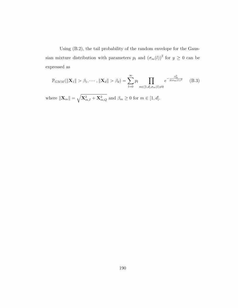
Using (B.2), the tail probability of the random envelope for the Gaus-
sian mixture distribution with parameters pl and (σm(l))2 for y ≥ 0 can be
expressed as
PGMM(‖X1‖ > β1, · · · , ‖Xd‖ > βd) =∞∑l=0
pl∏
m∈[1,d],σm(l)6=0
e− β2
m2(σm(l))2 (B.3)
where ‖Xm‖ =√
X2m,I + X2
m,Q and βm ≥ 0 for m ∈ [1, d].
190

Appendix C
Statistical Properties of Middleton Class A
Complex Random Variables
The Middleton Class A distribution is a particular form of the Gaussian
mixture distribution. The joint probability density function of a isotropic
complex random variable X = XI + jXQ distributed according to Middleton
Class A model (without an additive Gaussian component) can be expressed
as [13]
fXI ,XQ(XI , XQ) = e−Aδ(XI , XQ) +
∞∑m=1
e−AAm
m!e−X2I+X2
Q2mΩ2AA (C.1)
where A is the overlap index and Ω2A is the mean intensity of the random
variable.
From (C.1), the joint characteristic function of the in-phase and quadra-
ture phase components of the complex random variable can be expressed as
ΦXI ,XQ(ωI , ωQ) = e
A
e−(ω2I+ω2
Q)Ω2A2A −1
. (C.2)
Note that as A → ∞ while Ω2A is finite, the Middleton Class A model con-
verges to a Gaussian distribution with variance Ω2A.
Using (C.1), the tail probability for the Middleton Class A distribution
with parameters A and Ω2A corresponding to an amplitude threshold y ≥ 0
191

can be expressed as
PMCA(‖X‖ > β) =∞∑m=1
e−AAm
m!e− β2
2mΩ2AA . (C.3)
192

Bibliography
[1] R. Baldick, Applied Optimization: Formulation and Algorithms for En-
gineering Systems. Cambridge University Press, 2006.
[2] W. Liu, P. P. Pokharel, and J. C. Principe, “Correntropy: Properties and
applications in non-Gaussian signal processing,” IEEE Transactions on
Signal Processing, vol. 55, no. 11, pp. 5286–5298, 2007.
[3] J. G. Gonzalez, J. L. Paredes, and G. R. Arce, “Zero-order statistics: A
mathematical framework for the processing and characterization of very
impulsive signals,” IEEE Transactions on Signal Processing, vol. 54,
no. 10, pp. 3839–3851, Oct. 2006.
[4] L. . Cohen, “The history of noise,” IEEE Signal Processing Magazine,
vol. 22, no. 6, pp. 20–45, Nov. 2005.
[5] M. Schwartz, “Improving the noise performance of communication sys-
tems: radio and telephony developments of the 1920s,” IEEE Commu-
nications Magazine, vol. 47, no. 12, pp. 16–20, Dec. 2009.
[6] W. Schottky, “Uber spontane stromschwankungen in verschiedenen elek-
trizitatsleitern,” Annalen der Physik, vol. 362, no. 23, pp. 541–567,
1918.
193

[7] S. O. Rice, “Mathematical analysis of random noise,” Bell Systems Tech-
nical Journal, vol. 23, pp. 282–332, 1944.
[8] J. B. Johnson, “Electronic noise: the first two decades,” IEEE Spectrum,
vol. 8, no. 2, pp. 42–46, Feb. 1971.
[9] P. Gupta and P. R. Kumar, “The capacity of wireless networks,” IEEE
Transactions on Information Theory, vol. 46, no. 2, pp. 388–404, Mar.
2000.
[10] A. Kamerman and N. Erkocevic, “Microwave oven interference on wire-
less LANs operating in the 2.4 GHz ISM band,” in Proc. IEEE Inter-
national Symposium on Personal, Indoor and Mobile Radio Communi-
cations, vol. 3, Helsinki , Finland, Sep. 1–4 1997, pp. 1221–1227.
[11] K. Slattery and H. Skinner, Platform Interference in Wireless Systems:
Models, Measurement, and Mitigation. Newnes (Elsevier) Publishing,
2008.
[12] D. Middleton, “Statistical–physical models of man–made and natural
radio noise part II: First order probability models of the envelope and
phase,” U.S. Department of Commerce, Office of Telecommunications,
Tech. Rep., Apr. 1976.
[13] ——, “Non-Gaussian noise models in signal processing for telecommuni-
cations: New methods and results for class A and class B noise models,”
194

IEEE Transactions on Information Theory, vol. 45, no. 4, pp. 1129–
1149, May 1999.
[14] A. Goldsmith, Wireless Communications. Cambridge University Press,
2005.
[15] M. S. Alouini and A. J. Goldsmith, “Area spectral efficiency of cellu-
lar mobile radio systems,” IEEE Transactions on Vehicular Technology,
vol. 48, no. 4, pp. 1047–1065, July 1999.
[16] 3rd Generation Partnership Project (3GPP), Technical Specification Group
Radio Access Network; Physical layer aspects for evolved Universal Ter-
restrial Radio Access (E-UTRA), 3rd ed., March 2011.
[17] J. M. Peha, “Wireless communications and coexistence for smart envi-
ronments,” IEEE Personal Communications, vol. 7, no. 5, pp. 66–68,
Oct. 2000.
[18] IEEE ComSoc LAN MAN Standards Committee, Wireless LAN Medium
Access Control (MAC) and Physical Layer (PHY) Specifications: IEEE
Standard 802.11, The Institute of Electrical and Electronics Engineers,
1997.
[19] Bluetooth SIG, Core Specification of the Bluetooth System, v2.1 + edr ed.,
Jul. 2007.
[20] IEEE 802.15.4 Standard, Wireless medium access control (MAC) and
physical layer (PHY) specifications for low-rate Wireless Personal Area
195

Networks (LR-WPANs), The Institute of Electrical and Electronics En-
gineers, 2003.
[21] ZigBee Alliance, Zigbee Specification Document 053474, revision 14 ed.,
Nov. 2006.
[22] C. F. Chiasserini and R. R. Rao, “Coexistence mechanisms for interfer-
ence mitigation between IEEE 802.11 WLANs and Bluetooth,” in Proc.
IEEE International Conference on Computer Communications, vol. 2,
Nov. 2002, pp. 590–598.
[23] IEEE ComSoc LAN MAN Standards Committee, IEEE Standard for
Local and metropolitan area networks - Part 16: Air Interface for Broad-
band Wireless Access Systems, IEEE Std 802.16-2009 ed., The Institute
of Electrical and Electronics Engineers, May 2009.
[24] J. Zhu and H. Yin, “Enabling collocated coexistence in IEEE 802.16
networks via perceived concurrency,” IEEE Communications Magazine,
vol. 47, no. 6, pp. 108–114, Jun. 2009.
[25] Federal Communications Commission, Code of Federal Regulations -
Part 15 : Radio Frequency Device, 47th ed., Oct 2009.
[26] K. Blackard, T. Rappaport, and C. Bostian, “Measurements and models
of radio frequency impulsive noise for indoor wireless communications,”
IEEE Journal on Selected Areas in Communications, vol. 11, no. 7, pp.
991–1001, Sep. 1993.
196

[27] Y. Zhao, B. Agee, and J. Reed, “Simulation and measurement of mi-
crowave oven leakage for 802.11 WLAN interference management,” in
Proc. IEEE International Symposium on Microwave, Antenna, Prop-
agation and EMC Technologies for Wireless Communications, vol. 2,
Beijing, Aug. 2005, pp. 1580–1583.
[28] J. Shi, A. Bettner, G. Chinn, K. Slattery, and X. Dong, “A study of
platform EMI from LCD panels - impact on wireless, root causes and
mitigation methods,” in IEEE International Symposium on Electromag-
netic Compatibility, vol. 3, Portland, Oregon, Aug. 2006, pp. 626–631.
[29] A. Spaulding and D. Middleton, “Optimum reception in an impulsive
interference enviroment-part I: Coherent detection,” IEEE Transactions
on Communications, vol. 25, no. 9, pp. 910–923, 1977.
[30] J. G. Andrews, “Interference cancellation for cellular systems: A contem-
porary overview,” IEEE Wireless Communications Magazine, vol. 12,
no. 2, pp. 19–29, Apr. 2005.
[31] J. G. Andrews, N. Jindal, M. Haenggi, R. Berry, S. Jafar, D. Guo,
S. Shakkottai, R. W. Heath, M. Neely, S. Weber, and A. Yener, “Re-
thinking information theory for mobile ad hoc networks,” IEEE Com-
munications Magazine, vol. 46, no. 12, pp. 94–101, Dec. 2008.
[32] V. Chandrasekhar, J. G. Andrews, and A. Gatherer, “Femtocell net-
works: a survey,” IEEE Communications Magazine, vol. 46, no. 9, pp.
59–67, Sep. 2008.
197

[33] V. MacDonald, “The cellular concept,” Bell Systems Techical Journal,
vol. 58, no. 1, pp. 15–41, Jan. 1979.
[34] Nokia Siemens Networks, LTE Performance for initial deployments,
2009. [Online]. Available: www.nokiasiemensnetworks.com/sites/
default/files/document/LTE measurement A4 1302 0.pdf
[35] D. Cox, “Cochannel interference considerations in frequency reuse small-
coverage-area radio systems,” IEEE Transactions on Communications,
vol. 30, no. 1, pp. 135–142, Jan 1982.
[36] P. S. Jha, “Frequency reuse scheme with reduced co-channel interference
for fixed cellular systems,” in Proc. IEEE Electronic Letters, vol. 34,
no. 3, Feb 1998, pp. 237–238.
[37] E. Kuruoglu, “Signal processing in alpha stable environments: A least
lp approach,” Ph.D. dissertation, University of Cambridge, 1998.
[38] R. S. Blum, R. J. Kozick, and B. Sadler, “An adaptive spatial diversity
receiver for non-Gaussian interference and noise,” IEEE Transactions on
Signal Processing, vol. 47, no. 8, pp. 2100–2111, Aug. 1999.
[39] J. Haring and A. J. H. Vinck, “Iterative decoding of codes over complex
numbers for impulsive noise channels,” IEEE Transactions on Informa-
tion Theory, vol. 49, no. 5, pp. 1251–1260, May 2003.
198

[40] ——, “Coding and signal space diversity for a class of fading and impul-
sive noise channels,” IEEE Transactions on Information Theory, vol. 50,
no. 5, pp. 887–895, May 2004.
[41] P. Gao and C. Tepedelenlioglu, “Space-time coding over fading channels
with impulsive noise,” IEEE Transactions on Wireless Communications,
vol. 6, no. 1, pp. 220–229, Jan 2007.
[42] M. A. Maddah-Ali, A. S. Motahari, and A. K. Khandani, “Signaling over
MIMO multi-base systems: Combination of multi-access and broadcast,”
in Proc. IEEE International Symposium on Information Theory, Jul. 9–
14 2006, pp. 2104–2108.
[43] V. R. Cadambe and S. A. Jafar, “Interference alignment and degrees
of freedom of the k-user interference channel,” IEEE Transactions on
Information Theory, vol. 54, no. 8, pp. 3425–3441, Aug. 2008.
[44] C. Suh and D. Tse, “Interference alignment for cellular networks,” in
Proc. Allerton Conference on Communication, Control, and Computing,
Sep. 23–26 2008, pp. 1037–1044.
[45] U. Niesen, “Interference alignment in dense wireless networks,” in Proc.
IEEE Information Theory Workshop, Cairo, Jan. 6–8 2010, pp. 1–5.
[46] R. Tresch and M. Guillaud, “Performance of interference alignment in
clustered wireless ad hoc networks,” in Proc. IEEE International Sym-
posium on Information Theory, Jun. 13–18 2010, pp. 1703–1707.
199

[47] H. Zhou and T. Ratnarajah, “A novel interference draining scheme for
cognitive radio based on interference alignment,” in Proc. IEEE Sym-
posium on New Frontiers in Dynamic Spectrum, Apr. 6–9 2010, pp.
1–6.
[48] R. Tresch, M. Guillaud, and E. Riegler, “On the achievability of inter-
ference alignment in the k-user constant MIMO interference channel,” in
Proc. IEEE Workshop on Statistical Signal Processing, Aug. 31 – Sep.
3 2009, pp. 277–280.
[49] O. El Ayach, S. Peters, and R. W. Heath, “The feasibility of interference
alignment over measured MIMO-OFDM channels,” IEEE Transactions
on Vehicular Technology, vol. 59, no. 9, pp. 4309–4321, Nov. 2010.
[50] R. T. Krishnamachari and M. K. Varanasi, “Interference alignment un-
der limited feedback for MIMO interference channels,” in Proc. IEEE
International Symposium on Information Theory, Jun. 13–18 2010, pp.
619–623.
[51] G. J. Foschini, “Layered space-time architecture for wireless communica-
tion in a fading environment when using multi-element antennas,” Bell
Labs Technical Journal, vol. 1, no. 2, pp. 41–59, 1996.
[52] S. Verdu, Multiuser Detection. Cambridge University Press, 1998.
[53] S. Weber, J. G. Andrews, X. Yang, and G. de Veciana, “Transmission
capacity of wireless ad hoc networks with successive interference cancel-
200

lation,” IEEE Transactions on Information Theory, vol. 53, no. 8, pp.
2799–2814, Aug. 2007.
[54] K. Huang, J. G. Andrews, R. W. Heath Jr., D. Guo, and R. Berry,
“Spatial interference cancellation for multi-antenna mobile ad hoc
networks,” IEEE Transactions on Information Theory, Jul. 2008,
submitted. [Online]. Available: arxiv.org/pdf/0807.1773
[55] F. Baccelli, B. B laszczyszyn, and P. Muhlethaler, “An Aloha protocol for
multihop mobile wireless networks,” IEEE Transaction on Information
Theory, vol. 52, no. 2, pp. 412–436, Sep. 2006.
[56] A. Hasan, “Interference suppression in wireless ad hoc networks,” Ph.D.
dissertation, The University of Texas at Austin, May 2006.
[57] M. Kaynia, G. E. Oien, and N. Jindal, “Joint transmitter and receiver
sensing capability of CSMA in MANETs,” in Proc. IEEE International
Conference on Wireless Communications and Signal Processing, Nan-
jing, China, Nov. 2009.
[58] I. C. Wong, “A unified framework for optimal resource allocation in mul-
tiuser multicarrier wireless systems,” Ph.D. dissertation, The University
of Texas at Austin, May 2007.
[59] J. G. Andrews and A. Hasan, “Old standard new use,” IEE Communi-
cations Engineer, vol. 2, no. 1, pp. 22–26, Feb. 2004.
201

[60] A. Hasan and J. G. Andrews, “The guard zone in wireless ad hoc net-
works,” IEEE Transactions on Wireless Communications, vol. 4, no. 3,
pp. 897–906, Mar. 2007.
[61] H. Inaltekin, S. B. Wicker, M. Chiang, and H. V. Poor, “On unbounded
path-loss models: effects of singularity on wireless network performance,”
IEEE Journal on Selected Areas in Communications, vol. 27, no. 7, pp.
1078–1092, Sep. 2009.
[62] F. Baccelli, M. Klein, M. Lebourges, and S. Zuyev, “Stochastic geometry
and architecture of communication networks,” Journal of Telecommuni-
cation Systems, vol. 7, pp. 209–227, Jun. 1997.
[63] M. Haenggi and R. K. Ganti, “Interference in large wireless networks,”
in Foundations and Trends in Networking. Now Publishers Inc., Dec.
2008, vol. 3, no. 2, pp. 127–248.
[64] M. Z. Win, P. C. Pinto, and L. A. Shepp, “A mathematical theory
of network interference and its applications,” Proceedings of the IEEE,
vol. 97, no. 2, pp. 205–230, Feb. 2009.
[65] E. Salbaroli and A. Zanella, “Interference analysis in a Poisson field
of nodes of finite area,” IEEE Transactions on Vehicular Technology,
vol. 58, no. 4, pp. 1776–1783, May 2009.
[66] A. Rabbachin, T. Q. Quek, H. Shin, and M. Z. Win, “Cognitive network
interference,” IEEE Transactions on Selected Areas in Communications,
202

vol. 29, no. 2, pp. 480–493, Feb. 2011.
[67] F. Baccelli and B. B laszczyszyn, “Stochastic geometry and wireless net-
works, volume 1 — theory,” in Foundations and Trends in Networking.
Now Publishers Inc., March 2009, vol. 3, no. 3–4, pp. 249–449.
[68] ——, “Stochastic geometry and wireless networks, volume 2— applica-
tions,” in Foundations and Trends in Networking. Now Publishers Inc.,
March 2009, vol. 4, no. 1–2, pp. 1–312.
[69] F. Baccelli, M. Klein, M. Lebourges, and S. Zuyev, “Stochastic geom-
etry and architecture of communication networks,” Telecommunication
Systems, vol. 7, no. 1, pp. 209–227, 1997.
[70] E. S. Sousa, “Performance of a spread spectrum packet radio network
link in a Poisson field of interferers,” IEEE Transactions on Information
Theory, vol. 38, no. 6, pp. 1743–1754, Nov. 1992.
[71] J. Ilow and D. Hatzinakos, “Analytic alpha-stable noise modeling in a
Poisson field of interferers or scatterers,” IEEE Transactions on Signal
Processing, vol. 46, no. 6, pp. 1601–1611, Jun. 1998.
[72] X. Yang and A. Petropulu, “Co-channel interference modeling and anal-
ysis in a Poisson field of interferers in wireless communications,” IEEE
Transactions on Signal Processing, vol. 51, no. 1, pp. 64–76, Jan. 2003.
203

[73] K. F. McDonald and R. S. Blum, “A statistical and physical mechanisms-
based interference and noise model for array observations,” IEEE Trans-
actions on Signal Processing, vol. 48, pp. 2044–2056, Jul. 2000.
[74] M. Haenggi, J. G. Andrews, F. Baccelli, O. Dousse, and M. Franceschetti,
“Stochastic geometry and random graphs for the analysis and design of
wireless networks,” IEEE Journal on Selected Areas of Communications,
vol. 27, no. 7, pp. 1029–1046, Sep. 2009.
[75] R. Ganti and M. Haenggi, “Interference and outage in clustered wireless
ad hoc networks,” IEEE Transactions on Information Theory, vol. 55,
no. 9, pp. 4067–4086, Sep. 2009.
[76] S. Weber, J. G. Andrews, and N. Jindal, “An overview of the transmis-
sion capacity of wireless networks,” IEEE Transactions on Communica-
tions, vol. 58, no. 12, pp. 3593–3604, Dec. 2010.
[77] X. Yang and G. de Veciana, “Inducing multiscale spatial clustering us-
ing multistage MAC contention in spread spectrum ad hoc networks,”
IEEE/ACM Transactions on Networking, vol. 15, no. 6, pp. 1387–1400,
Dec. 2007.
[78] M. Haenggi, “Outage, local throughput, and capacity of random wire-
less networks,” IEEE Transactions on Wireless Communications, vol. 8,
no. 8, pp. 4350–4359, Aug. 2009.
204

[79] R. K. Ganti and J. G. Andrews, “A new method for computing the
transmission capacity of non-Poisson wireless networks,” in Proc. IEEE
International Symposium on Information Theory, Austin, TX, Jun. 13–
18 2010, pp. 1693–1697.
[80] M. Franceschetti, M. D. Migliore, and P. Minero, “The capacity of wire-
less networks: Information-theoretic and physical limits,” IEEE Trans-
actions on Information Theory, vol. 55, no. 8, pp. 3413–3424, Aug.
2009.
[81] M. Franceschetti, O. Dousse, D. Tse, and P. Thiran, “Closing the gap in
the capacity of wireless networks via percolation theory,” IEEE Trans-
actions on Information Theory, vol. 53, no. 3, pp. 1009–1018, Mar.
2007.
[82] R. Negi and A. Rajeswaran, “Capacity of power constrained ad-hoc net-
works,” in Proc. IEEE Conference on Computer Communications, Hong
Kong, May 2004, pp. 443–453.
[83] M. Grossglauser and D. Tse, “Mobility increases the capacity of adhoc
wireless networks,” IEEE/ACM Transactions on Networking, vol. 10,
no. 4, pp. 477–486, Aug. 2002.
[84] J. G. Andrews, S. Weber, M. Kountouris, and M. Haenggi, “Random
access transport capacity,” IEEE Transactions On Wireless Communi-
cations, vol. 9, no. 6, pp. 2101–2111, Jun. 2010.
205

[85] U. Niesen, P. Gupta, and D. Shah, “The balanced unicast and multi-
cast capacity region of large wireless networks,” IEEE Transactions on
Information Theory, vol. 56, no. 5, pp. 2249–2271, May 2010.
[86] L. Xie and P. R. Kumar, “A network information theory for wireless
communication: Scaling laws and optimal operation,” IEEE Transac-
tions on Information Theory, vol. 50, no. 5, pp. 748–767, May 2004.
[87] S. Weber, X. Yang, J. G. Andrews, and G. de Veciana, “Transmission
capacity of wireless ad hoc networks with outage constraints,” IEEE
Transactions on Information Theory, vol. 51, no. 12, pp. 4091–4102,
Dec. 2005.
[88] S. Weber, J. G. Andrews, and N. Jindal, “The effect of fading, channel
inversion, and threshold scheduling on ad hoc networks,” IEEE Trans-
actions on Information Theory, vol. 53, no. 11, pp. 4127–4149, Nov.
2007.
[89] A. M. Hunter, J. G. Andrews, and S. P. Weber, “Transmission capacity of
ad hoc networks with spatial diversity,” IEEE Transactions on Wireless
Communications, vol. 7, no. 12, pp. 5058–5071, Dec. 2008.
[90] R. Vaze and J. R. W. Heath, “Transmission capacity of multiple antenna
ad-hoc networks without channel state information at the transmitter
and interference cancelation at the receiver,” in Proc. IEEE Asilomar
Conference on Signals, Systems, and Computers, Pacific Grove, CA,
Nov. 1–4 2009.
206

[91] R. Vaze, “Throughput-delay-reliability tradeoff in ad hoc networks,”
in Workshop on Spatial Stochastic Models for Wireless Networks, Jun.
2010.
[92] M. Haenggi, “Local delay in static and highly mobile Poisson networks
with ALOHA,” in Proc. IEEE International Conference on Communi-
cations, Cape Town, South Africa, May 2010.
[93] ——, “Local delay in Poisson networks with and without interference,”
in Proc. Allerton Conference on Communication, Control, and Comput-
ing, Sep. 29 – Oct. 1 2010.
[94] F. Baccelli and B. B laszczyszyn, “A new phase transition for local delays
in MANETs,” in Proc. IEEE International Conference on Computer
Communications, San Diego, CA, Mar. 14–19 2010, pp. 1–9.
[95] G. Alfano, R. Tresch, and M. Guillaud, “Spatial diversity impact on the
local delay of homogeneous and clustered wireless networks,” in Proc.
IEEE International Workshop on Smart Antennas, Aachen, Germany,
Feb. 24–25 2011, pp. 1–6.
[96] J. Haring and A. J. H. Vinck, “Performance bounds for optimum and
suboptimum reception under class-A impulsive noise,” IEEE Transac-
tions for Communications, vol. 50, no. 7, pp. 1130–1136, Jul. 2002.
[97] S. V. Zhidkov, “Analysis and comparison of several simple impulsive
noise mitigation schemes for OFDM receivers,” IEEE Transactions on
207

Communications, vol. 56, no. 1, pp. 5–9, Jan. 2008.
[98] K. Gulati, A. Chopra, R. W. Heath, B. L. Evans, K. R. Tinsley, and
X. E. Lin, “MIMO receiver design in the presence of radio frequency
interference,” in Proc. IEEE Global Communications Conference, New
Orleans, LA, Nov. 30–Dec. 4 2008.
[99] M. Nassar, K. Gulati, M. DeYoung, B. L. Evans, and K. R.
Tinsley, “Mitigating near-field interference in laptop embedded wireless
transceivers,” Journal of Signal Processing Systems, Mar. 2009.
[Online]. Available: http://dx.doi.org/10.1007/s11265-009-0350-7
[100] P. J. Huber, Robust Statistics. John Wiley & Sons, 1981.
[101] G. R. Arce, Nonlinear Signal Processing: A Statistical Approach. John
Wiley & Sons, 2005.
[102] S. Ambike, J. Ilow, and D. Hatzinakos, “Detection for binary transmis-
sion in a mixture of Gaussian noise and impulsive noise modeled as an
alpha-stable process,” IEEE Signal Processing Letters, vol. 1, no. 3, pp.
55–57, Mar. 1994.
[103] H. Vikalo, B. Hassibi, and T. Kailath, “On robust multiuser detection,”
in Proc. Asilomar Conference on Signals, Systems and Computers, no.
Nov., 29 Oct .–1 Nov. 2000, pp. 1168 –1172.
[104] K. Gulati, B. L. Evans, J. G. Andrews, and K. R. Tinsley, “Statis-
tics of co-channel interference in a field of Poisson and Poisson-Poisson
208

clustered interferers,” IEEE Transactions on Signal Processing, vol. 58,
no. 12, pp. 6207–6222, Dec. 2010.
[105] J. Gonzalez, D. Griffith, and G. Arce, “Matched myriad filtering for
robust communications,” in Proc. Conference on Information Sciences
and Systems, 1996.
[106] J. G. Gonzalez, “Robust techniques for wireless communications in non-
Gaussian environments,” Ph.D. dissertation, University of Delaware,
Newark, 1997.
[107] J. G. Gonzalez and G. Arce, “Optimality of the myriad filter in practical
impulsive-noise environments,” IEEE Transactions on Signal Processing,
vol. 49, no. 2, pp. 438–441, Feb. 2001.
[108] C. L. Nikias and M. Shao, Signal Processing with Alpha-Stable Distribu-
tions and Applications. John Wiley & Sons, 1995.
[109] H. Ong and A. Zoubir, “Estimation and detection in a mixture of sym-
metric alpha stable and Gaussian interference,” in Proc. IEEE Sig-
nal Processing Workshop on High-Order Statistics, Madison, Wisconsin,
Jun. 14–16 1999.
[110] H. W. Sorenson and D. L. Alspach, “Recursive Bayesian estimation using
Gaussian sums,” Automatica, vol. 7, pp. 465–479, 1971.
209

[111] D. L. Alspach and H. W. Sorenson, “Nonlinear Bayesian estimation us-
ing Gaussian sum approximation,” IEEE Transactions on Automatic
Control, vol. 17, no. 4, pp. 439–448, Apr. 1972.
[112] Y. Eldar and A. Yeredor, “Finite-memory denoising in impulsive noise
using Gaussian mixture models,” IEEE Transactions on Circuits and
Systems II: Analog and Digital Signal Processing, vol. 48, no. 11, pp.
1069–1077, Nov. 2001.
[113] J. H. Kotecha and P. M. Djuric, “Gaussian sum particle filtering,” IEEE
Transactions on Signal Processing, vol. 51, no. 10, pp. 2602–2612, Oct.
2003.
[114] J. H. Miller and J. B. Thomas, “Detectors for discrete-time signals in
non-Gaussian noise,” IEEE Transactions on Information Theory, vol. 18,
pp. 241–250, Mar. 1972.
[115] J. Astola and Y. Neuvo, “Nonlinear median based receiver for QAM
signals,” in Proc. IEEE Global Telecommunications Conference, vol. 3,
San Diego, CA, Dec. 2–5 1990, pp. 2030–2034.
[116] N. C. Beaulieu and S. Niranjayan, “New UWB receiver designs based on
a Gaussian-Laplacian noise-plus-MAI model,” in Proc. IEEE Interna-
tional Conference on Communications, Glasgow, Jun. 24–28 2007, pp.
4128–4133.
210

[117] V. J. Mathews and G. L. Sicuranza, Polynomial Signal Processing. Wiley-
Interscience, 2000.
[118] V. Milosevic and B. Ristic, “Effect of impulse noise rejection with median
filter on binary digital receiver performance,” IEEE Electronic Letters,
vol. 25, no. 6, pp. 392–394, Mar. 1989.
[119] C. Nikias and A. P. Petropulu, Higher Order Spectra Analysis: A Non-
Linear Signal Processing Framework. Prentice Hall, 1993.
[120] B. M. Sadler, G. B. Giannakis, and K.-S. Lii, “Estimation and detection
in non-Gaussian noise using higher order statistics,” IEEE Transactions
on Signal Processing, vol. 42, no. 10, pp. 2729–2741, Oct. 1994.
[121] M. Janzura and T. Koski, “Minimum entropy of error principle in es-
timation,” Information Sciences, vol. 79, no. 1–2, pp. 123–144, Jul.
1994.
[122] K. Gulati, A. Chopra, B. L. Evans, and K. R. Tinsley, “Statistical mod-
eling of co-channel interference,” in Proc. IEEE Global Communications
Conference, Honolulu, Hawaii, Nov. 30–Dec. 4 2009.
[123] K. Gulati, B. L. Evans, and K. R. Tinsley, “Statistical modeling of co-
channel interference in a field of Poisson distributed interferers,” in Proc.
IEEE International Conference on Acoustics, Speech, and Signal Pro-
cessing, Dallas, TX, Mar. 14–19 2010, pp. 3490–3493.
211

[124] V. Chandrasekhar and J. G. Andrews, “Uplink capacity and interfer-
ence avoidance for two-tier femtocell networks,” IEEE Transactions on
Wireless Communications, vol. 8, no. 7, pp. 3498–3509, Jul. 2009.
[125] G. Samorodnitsky and M. S. Taqqu, Stable Non-Gaussian Random Pro-
cesses: Stochastic Models with Infinite Variance. Chapman and Hall,
New York, 1994.
[126] M. Westcott, “On the existence of a generalized shot-noise process,” in
Studies in Probability and Statistics: Papers in Honour of Edwin J. G.
Pitman, Amsterdam, 1976, pp. 73–88.
[127] S. B. Lowen and M. C. Teich, “Power-law shot noise,” IEEE Transac-
tions on Information Theory, vol. 36, no. 6, pp. 1302–1318, Nov. 1990.
[128] J. Venkataraman, M. Haenggi, and O. Collins, “Shot noise models for
outage and throughput analysis in wireless ad hoc networks,” in Proc.
Military Communications Conference, Oct. 2006, pp. 1–7.
[129] D. J. Daley and D. Vere-Jones, An Introduction to the Theory of Point
Processes, 1st ed. Springer, New York, 1988.
[130] Z. I. Botev, “A novel nonparametric density estimator,” The University
of Queensland, Australia, Tech. Rep., Nov. 2006.
[131] T. M. Cover and J. A. Thomas, Elements of Information Theory, 2nd ed.
Wiley & Sons, New York, 2006.
212

[132] R. K. Ganti and M. Haenggi, “Spatial and temporal correlation of the in-
terference in ALOHA ad hoc networks,” IEEE Communications Letters,
vol. 13, no. 9, pp. 631–633, Sep. 2009.
[133] S. Srinivasa and M. Haenggi, “Throughput-delay-reliability tradeoffs in
multihop networks with random access,” in Allerton Conference on Com-
munication, Control and Computing, Monticello, IL, Sep. 2010.
[134] S. S. Rappaport and L. Kurz, “An optimal nonlinear detector for digital
data transmission through non-Gaussian channels,” IEEE Transactions
on Communications Technology, vol. 14, no. 3, pp. 266–274, Jun. 1966.
[135] J. J. Sheehy, “Optimum detection of signals in non-Gaussian noise,”
Journal of Acoustical Society of America, vol. 63, no. 1, pp. 81–90, Jan.
1978.
[136] W. Liu, P. P. Pokharel, and J. C. Principe, “Error entropy, correntropy
and M-estimation,” in Proc. IEEE Workshop on Machine Learning for
Signal Processing, Arlington, VA, Sep. 6–8 2006, pp. 179–184.
[137] P. P. Pokharel, R. Agrawal, and J. C. Principe, “Correntropy based
matched filtering,” in Proc. IEEE Workshop on Machine Learning for
Signal Processing, 28 Sep. 2005, pp. 341–346.
[138] A. Singh and J. C. Principe, “Using correntropy as a cost function in
linear adaptive filters,” in Proc. IEEE International Joint Conference
on Neural Networks, Atlanta, GA, Jun. 14–19 2009, pp. 2950–2955.
213

[139] A. Kenarsari-Anhari and L. H. J. Lampe, “Performance analysis for
BICM transmission over Gaussian mixture noise fading channels,” IEEE
Transactions on Communications, vol. 58, no. 7, pp. 1962–1972, Jul.
2010.
[140] M. H. Hayes, Statistical Digital Signal Processing and Modeling. John
Wiley & Sons, 2006.
[141] D. Umehara, H. Yamaguchi, and Y. Morihiro, “Turbo decoding in im-
pulsive noise environment,” in Proc. IEEE Global Telecommunications
Conference, 29 Nov. – 3 Dec. 2004, pp. 194–198.
[142] D. Fertonani and G. Colavolpe, “A robust metric for soft-output detec-
tion in the presence of class-A noise,” IEEE Transactions on Communi-
cations, vol. 57, no. 1, pp. 36–40, Jan. 2009.
[143] R. K. Ganti, F. Baccelli, and J. G. Andrews, “Series expansion
for interference in wireless networks,” IEEE Transactions on
Information Theory, Jan. 2011, submitted. [Online]. Available:
http://arxiv.org/abs/1101.3824
[144] C. Lee and M. Haenggi, “Interference and outage in doubly Poisson cog-
nitive networks,” in Proc. IEEE International Conference on Computer
Communications and Networks, Aug. 2–5 2010.
[145] D. W. J. Stein, “Detection of random signals in Gaussian mixture noise,”
214

IEEE Transactions on Information Theory, vol. 41, no. 6, pp. 1788–
1801, Nov. 1995.
[146] M. Nassar, K. Gulati, Y. Mortazavi, and B. L. Evans, “Statistical mod-
eling of asynchronous impulsive noise in powerline communication net-
works,” in Proc. IEEE Global Communications Conference, Houston,
TX, Dec. 5–9 2011, submitted.
[147] J. Lin, M. Nassar, Y. Mortazavi, and B. L. Evans, “Combating channel
impairments and impulsive noise in local utility powerline communica-
tions,” IEEE Signal Processing Magazine, Apr. 2011, submitted.
[148] F. Abdelkefi, P. Duhamel, and F. Alberge, “Impulsive noise cancellation
in multicarrier transmission,” IEEE Transactions on Communications,
vol. 53, no. 1, pp. 94–106, Jan. 2005.
215

Vita
Kapil Gulati received the B.Tech. degree in Electronics and Commu-
nications Engineering from the Indian Institute of Technology, Guwahati in
May 2004 and the M.S. degree in Electrical Engineering from The University
of Texas at Austin in May 2008. From 2004 to 2006, he was employed as a
Hardware Design Engineer at Texas Instruments, India. He enrolled at The
University of Texas at Austin in Fall 2006. In Fall 2006, he was a teaching as-
sistant for the senior design projects course. Since Spring 2007, he has been a
research assistant at the Embedded Signal Processing Laboratory. In summer
2007 and 2008, he was a intern at Intel Labs in Santa Clara, California. He
co-authored a paper on his work at Intel Labs that won the best paper award
at the 2009 IEEE Computer Society Annual Symposium on VLSI, Tampa,
Florida. In summer 2010, he was a intern at Qualcomm Inc. in San Diego,
California. His research interests include mathematical modeling of wireless
networks and signal processing in the presence of non-Gaussian noise.
Permanent address: 1100 E 32 StreetAustin, Texas 78722
This dissertation was typeset with LATEX† by the author.
†LATEX is a document preparation system developed by Leslie Lamport as a specialversion of Donald Knuth’s TEX Program.
216


